the changing cyclical responsiveness of wage … · the changing cyclical responsiveness of wage...
TRANSCRIPT
MICHAEL L. WACHTER
University of Pennsylvania
The Changing Cyclical
Responsiveness
of Wage Infa0on
A POPULAR THEME in discussions of stabilization policy is that inflation -wage inflation, in particular-is becoming less responsive to changes in unemployment and to the forces of aggregate demand in general. The view is that wages today respond only slightly to unemployment and vary more closely with prices, which in turn depend most on cost variables. Since the cost variables are essentially prices (and wages are the most significant single price), the system reduces to a highly autoregressive model, with unemployment or demand seemingly playing a minor and shrinking role.
The government-engineered recession applied to cure inflation in 1969- 70 was judged to be a failure. This judgment has led many economists to argue that monetary and fiscal policy simply takes too long to slow infla- tion; and the 1973-74 slowdown and the sharper 1974-75 decline seem to reinforce these views. Some never believed that recessions significantly slowed inflation; others lost their faith in them after the late 1950s. Since the social costs presumably become larger the smaller the adjustment of wages to unemployment and to aggregate demand in general, the issue of "changing responsiveness" has become a central concern to policymakers and is the focus of this paper.
Note: I am grateful to the National Science Foundation and the National Institutes of Health for research support. Valuable comments were provided by members of the Brookings Panel on Economic Activity. I also wish to thank James Orr, Dennis Ahlburg, and Gail Moskowitz for research assistance.
115

116 Brookings Papers on Economic Activity, 1:1976
Table 1. Wage Coefficients of the Official Unemployment Rate and the Nonfarm Deflator, Various Periods, Beginning 1954:1
Inverse of the Percentage official unemployment change in
rate prices Period U-' pt-l
1954: 1-1965:4 3.9980 0.0627 -1968:4 4.9608 0.0650 -1969:4 5.2399 0.1058 -1971:4 2.6064 0.4884 -1973:4 2.1896 0.4371 -1975:2 2.3308 0.4414
Source: Derived from equation wvt ao + al Ut-1 + a2h t-l, where i,t = quarterly percentage change in the average hourly earnings index of private nonsupervisory workers, adjusted for overtime in manu- facturing and interindustry shifts; U-1 = inverse of the official unemployment rate; and 't-1 = quarterly percentage change in the nonfarm deflator, lagged one quarter.
My results run counter to the popular theme: in particular, I find that the influence of unemployment is greater today than it was in the 1950s. More specifically, the coefficient in the wage equation on the labor-market variable, UGAP (which I describe below), has increased over the post-1954 period. Not only is there more wage inflation, ceteris paribus, for any given level of labor-market tightness, but also the Phillips curve has become steeper and not flatter. To be sure, wage-inflation rates are still quite sticky since the estimated distributed lags are long.
A broad range of wage equations reveals the growing cyclical responsive- ness of wage inflation. Quasi-reduced-form wage equations, which include both UGAP and the percentage change in the money supply, explain wage inflation as well as models with autoregressive price and wage terms. Both have coefficients on UGAP that increase through time. The statistical success of the growth in the money supply as a variable substituting for prices provides evidence on the importance of aggregate demand in general and suggests that lagged prices in the structural wage equation should be interpreted as a distributed-lag generator of past demand effects. My re- sults also indicate that, if the full-employment unemployment rate was between 4 and 4.5 percent during the 1950s, then it is approximately 5.5 percent today. Thus, I find that the normalized full-employment rate (de- noted UN) is higher and that deviations from that rate have a heavier impact on inflation today than twenty years ago. In this paper, I make no attempt to find a new and more stable Phillips curve. Indeed, the coeffi- cients of the wage equations are assumed to change over time.

Michael L. Wachter 117
The results present intermediate-run danger signals for expansionary policy. In the near term there need be little concern for inflation, since unemployment is so high. If the full-employment unemployment rate is near 5.5 percent, however, it is higher than the perceived full-employment point that dominates current political debates. Since the parameters on the demand variables are larger today than in earlier periods, a recovery in which unemployment falls into the excess-demand zone, and in which, because of their lag, prices have had little time to adjust downward, should lead to the highest ongoing inflation rate in the postwar period. Over the near term, however, the larger parameters on the demand variables imply that progress can be made in moderating inflation. Within a few years, the inflation rate can be reduced if society is willing to pay the cost of high unemployment. However, the high level of the full-employment unem- ployment rate strongly suggests a need to implement structural measures to reduce UN as a complement to an expansionary aggregate-demand policy.
The Case for Increasing Rigidity
Although there has been little work that directly investigates the issue of changing responsiveness, some available evidence appears to support the view that the Phillips curve has become less steep. For example, esti- mates of a simplified Phillips curve equation, shown in table 1, indicate that the coefficient on U-1 (the reciprocal of the unemployment rate) drops by more than 50 percent between 1969 and 1975. Hence, the Phillips curve evolves into a practically horizontal line. At the same time, the coefficient on price inflation increases just as dramatically and as persistently. Al- though the Phillips curve of table 1 is a straw man when compared with the complicated specifications in the literature, a cataloguing of those various equations would yield essentially this conclusion with respect to the relevant coefficients. Unfortunately, direct comparisons across equa- tions are not possible because of differences in the specification of the relationship.
These observations have led some to adopt the view that the wage system is driven increasingly by prices rather than by demand pressures in the labor market. Making matters worse, the price equation has almost uniformly been estimated to follow costs, but not demand pressures, in the goods markets. The cost arguments in the price function, however,

118 Brookings Papers on Economic Activity, 1:1976
Table 2. Change in Compensation per Manhour in the Private Nonfarm Economy, Four Quarters before and after Cyclical Peaks, 1948-73
Change in compensation Difference( per manhourb (percentage
Period Cyclical peaka (percent) points)
Before peak 1948:4 8.0 After peak 0.4
Difference -7.6
Before peak 1953:2 6.0 After peak 3.3
Difference -2.7
Before peak 1957:3 5.4 After peak 3.8
Difference -1.6
Before peak 1960:2 4.3 After peak 3.0
Difference -1.3
Before peak 1969:4 6.7 After peakd 7.4
Difference 0.7
Before peak 1973:4 8.0p After peak 9.7p
Difference 1.7p Source: Economic Report of the President, February 1975, together with the Annual Report of the Council
of Economic Advisers, p. 140. a. Quarter designated as cyclical peak by National Bureau of Econoomic Research. b. Four-quarter rate of change; all persons. c. All differences, except as noted, are changes four quarters after peak minus changes four quarters
before peak. d. Change from 1969:4 to average of 1970:4 and 1971 :1 to smooth effect of auto strike. p Prelinminary.
are simply other prices, such as those of capital, labor (the wage rate), and raw materials.'
What emerges in this context is an autoregressive system in which wages (and prices) follow some combination of their own lagged values. For my
1. See the review article by William D. Nordhaus, "Recent Developments in Price Dynamics," in Otto Eckstein, ed., The Econometrics of Price Determination, A Con- ference Sponsored by the Board of Governors of the Federal Reserve System and the Social Science Research Council (Board of Governors, 1972), and George de Menil, "Aggregate Price Dynamics," Review of Economics and Statistics, vol. 56 (May 1974), pp. 129-40. That demand variables may be important-even in a cost-driven price equa- tion-is shown by Robert J. Gordon, "The Impact of Aggregate Demand on Prices," BPEA, 3:1975, pp. 613-70. If one adopts the methodology that I use here in the wage equation, one would almost certainly find a much greater role for demand pressures in the price equation.

Michael L. Wachter 119
purposes it is not important whether wages are determined by lagged wages or lagged prices or some combination of the two. Any of these relations is an essentially autoregressive form in which demand forces are absent or have little effect. In the extreme, these models are akin to a natural-rate theory of wage inflation. Wages are exogenous in that they are determined in an autoregressive model. Rather than being vertical, the Phillips curve is horizontal.2
A second piece of evidence is found by analyzing changes in wages from the peak to the trough of business cycles. Appearing in the 1975 Annual Report of the Council of Economic Advisers were the data shown in table 2, which indicate that the deceleration in wage inflation immedi- ately before and after peaks has been dampened considerably since 1945. For example, the rise in compensation per manhour slowed 7.6 percentage points between the 1948 peak (when the rate was 8.0 percent) and a year later (0.4 percent). By the 1960 downturn the wage deceleration around the peak was only 1.3 points and after the 1969 peak, wage inflation actually accelerated. In an excellent study of price changes over the business cycle, Philip Cagan presents a detailed analysis of price responsiveness going back to cyclical swings during the 1920s. Here again, the evidence appears to suggest that prices have responded less to excess supply in postwar recessions than in prewar ones and similarly less in the more recent post- war recessions than in the earlier postwar experiences.3
2. The view that the wage-price or wage-wage process can proceed with little or no impact from demand factors has surfaced regularly during the discussions of inflation at the Brookings panel meetings. See, for example, "General Discussion" (of papers by Barry Bosworth and Robert J. Gordon), BPEA, 2:1972, pp. 426-30. A more moderate stance, but one still stressing the weakness of demand factors, is taken in Arthur M. Okun, "Inflation: Its Mechanics and Welfare Costs," BPEA, 2:1975, pp. 369-72; William D. Nordhaus, "Inflation Theory and Policy," American Economic Review, vol. 66 (May 1976), pp. 59-64; and U.S. Congressional Budget Office, "Recovery: How Fast and How Far" (Government Printing Office, 1975; processed). One of the earliest post-Keynesian models in which changes in wage inflation are not, and never were, caused by aggregate demand can be found in Sidney Weintraub, Al Approach to the Theory of Income Distribution (Chilton, 1958).
3. Phillip Cagan, The Hydra-Headed Monster: Thze Problem of Inflation in the United States (American Enterprise Institute, 1974). Cagan concludes that "the dampened response appears to reflect ... a strengthened, general belief that inflationary move- ments will not be subdued quickly" (p. 48). This, he argues, is due in turn to the govern- ment's commitment to full employment unconstrained by gold-reserve requirements. See also his "Changes in the Recession Behavior of Wholesale Prices in the 1920's and Post-World War II," Explorations in Economic Research, vol. 2 (Winter 1975), pp. 54-104. The Cagan discussion is not couched in the Phillips-curve terminology, and he appears to be discussing aggregate demand in general.

120 Brookings Papers on Economic Activity, 1:1976
General Background
The issue of the increasing responsiveness of wages involves four ele- ments: the problem of differentiating movements along a Phillips curve from shifts in the curve, the interpretation of predetermined variables in the wage equation, the dating of cyclical turning points for wage inflation, and the definition of the proper unemployment variable. In order to elabo- rate on these points, I first sketch out the underlying wage model to be tested and then explore briefly the basis of wage rigidity.
THE WAGE EQUATION
The basic wage equation, excluding for the moment the question of the variation over time in the slope of the Phillips curve, is of the form
(1) Wi't = ao + E f 3UGAP ti + yIp yt-i + El, i=O i=l
where wi is the percentage rate of change of wages, UGAP is some measure of labor-market tightness (to be defined below), and p3 is the percentage rate of change of prices. The error term, El, is assumed to be serially un- correlated and normally distributed. The distributed lags are important because the firm's labor market is, in general, not an auction market that adjusts to daily spot wages. Rather, as discussed below, the firm is best viewed as adopting a wage strategy (for example, a fixed schedule of future wage increases) for some planning period. The clearest case of this concept is the multiyear union contract.
In the traditional Phillips-curve equation, lags are included on the price term but not on the unemployment term. This is an unnecessarily restric- tive assumption since the fixed-wage contract makes conditions in the labor market at t- i relevant to wage changes contracted in the current period, t. More generally, then, lags should be included on both p and UGAP to represent an amalgam of expectational and adjustment effects.
In analyzing the responsiveness of wage inflation to unemployment, attention is usually focused on 300, the current coefficient of UGAP. Adding a distributed lag on UGAP makes it clear that the direct effect of unem- ployment on wages should include the full term ioi.
Besides the direct effect, loi, unemployment, or UGAP, also has an in-

Michael L. Wachter 121
direct effect on iw through the price equation. Most price equations are written as a cost markup with demand playing a small role. A fairly general price equation is of the form
(2) fit = 0 + 0C16 +02(V-4) + q3D+ E2,
where e is a vector of cost variables, excluding wages, q is the percentage rate of change of long-run productivity, and D is a demand variable, such as capacity utilization.
Even if one assumes that p3 is small or close to zero, equation 2 indi- cates an indirect effect of unemployment on wage inflation. Specifically, if equations 1 and 2 are solved for a reduced-form equation, what results is an indirect or feedback effect through the influence of iw on p.4 Indeed, the feedback effect indicates that the wage equation can be written as a func- tion of an infinite lagged time series of the unemployment rate. Interpreted in this manner, the price term in the structural wage equation acts as a distributed-lag generator for the independent variable UGAP.5
Consequently, identifying short- and long-run responses is central to the question of the responsiveness of wage inflation to aggregate demand. The term 10i (and not just the initial coefficient, 3oo) measures the short-run or direct effect. The feedback response of demand variables through the price mechanism represents the long-run or indirect effect. The reduced- form specification, in which wv is a function of UGAP with an infinite lag, makes it clear that the point at which the direct unemployment lag ends and the indirect effect begins is a matter of definition.
To test for the changing responsiveness of wage inflation to unemploy- ment or to aggregate demand in general, the parameters of equation 1 are allowed to vary over time, r. In general form, the wage equation may be written as
m n
(3) Wt-= ao() + E 3(Tr)UGAP t- + E -Yi(r)pt-i + El. i=O i=1
4. In the long run, if the Phillips curve is vertical, the structural wage-price-unem- ployment equations cannot be solved to yield a quasi-reduced-form wage equation. The fact that wages and unemployment are always observed in short-run disequilibrium allows estimation of the Phillips relationship.
5. If the autoregressive term is viewed as a distributed-lag generator for the labor- market term, then it makes less difference whether UGAP is entered with or without a lag. Placing a lag on UGAP, in combination with one on p, only increases the flexi- bility of the lag structure that links w to lagged aggregate-demand effects. This point appears in the empirical results below.
122 Brookings Papers on Economic Activity, 1:1976
Specifically, for estimation purposes, I adopt the assumption that changes in parameters have proceeded monotonically (following a trend).
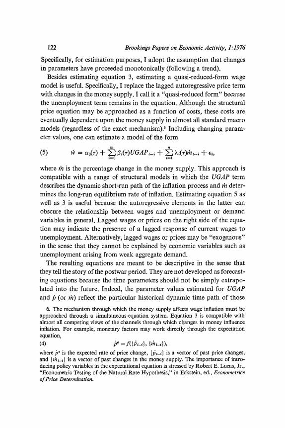
Besides estimating equation 3, estimating a quasi-reduced-form wage model is useful. Specifically, I replace the lagged autoregressive price term with changes in the money supply. I call it a "quasi-reduced form" because the unemployment term remains in the equation. Although the structural price equation may be approached as a function of costs, these costs are eventually dependent upon the money supply in almost all standard macro models (regardless of the exact mechanism).6 Including changing param- eter values, one can estimate a model of the form
mn
(5) = ao(T) + , 3(&r)UGAPti + E X)i(r)itizt + E3,
where im is the percentage change in the money supply. This approach is compatible with a range of structural models in which the UGAP term describes the dynamic short-run path of the inflation process and mh deter- mines the long-run equilibrium rate of inflation. Estimating equation 5 as well as 3 is useful because the autoregressive elements in the latter can obscure the relationship between wages and unemployment or demand variables in general. Lagged wages or prices on the right side of the equa- tion may indicate the presence of a lagged response of current wages to unemployment. Alternatively, lagged wages or prices may be "exogenous" in the sense that they cannot be explained by economic variables such as unemployment arising from weak aggregate demand.
The resulting equations are meant to be descriptive in the sense that they tell the story of the postwar period. They are not developed as forecast- ing equations because the time parameters should not be simply extrapo- lated into the future. Indeed, the parameter values estimated for UGAP and p3 (or m1) reflect the particular historical dynamic time path of those
6. The mechanism through which the money supply affects wage inflation must be approached through a simultaneous-equation system. Equation 3 is compatible with almost all competing views of the channels through which changes in money influence inflation. For example, monetary factors may work directly through the expectation equation,
(4) e=f P_} m_})
where pe is the expected rate of price change, {jti} is a vector of past price changes, and 1t'i-i} is a vector of past changes in the money supply. The importance of intro- ducing policy variables in the expectational equation is stressed by Robert E. Lucas, Jr., "Econometric Testing of the Natural Rate Hypothesis," in Eckstein, ed., Econometrics of Price Determination.

Michael L. Wachter 123
variables. For example, the statistical importance of prices relative to unemployment over any data set depends upon the character of cyclical fluctations. If unemployment moves back and forth across the noninfla- tionary rate, but never too far in either direction (perhaps because the government pursues a dampened stop-go policy), then the unemployment term will be statistically most significant because the observations will be around a narrow band of Phillips curves. Indeed, any p term may well be insignificant due to a lack of independent variation.
THE CAUSES OF WAGE INSENSITWITY
In a noncyclical setting, wage rigidity has two components: one origi- nates from firms-the wage offered; the other from workers-the reserva- tion wage. Since I have discussed my own position on the wage-rigidity question elsewhere, and since Okun and Hall7 have advanced or extended the general type of model significantly in a recent issue of Brookings Papers, I will deal with the topic only briefly here.
Firms pay a wage premium for their work force for a variety of reasons, which arise from two types of phenomena. The first is the presence of unions and oligopolies. Unions desire a wage premium as an end in itself whereas oligopolies use it to assure a labor supply and, in particular, a queue of workers for periods of demand expansion.8 The second, inter- related, phenomenon is the desire of firms for an ongoing relationship with their workforce, especially where the job content is idiosyncratic and involves considerable job-specific training.9 As a consequence, most jobs in these high-wage firms do not have a direct demand-and-supply component. Rather, they are part of the internal labor market of the firm in which jobs are connected through a series of promotion ladders with
7. Okun, "Inflation: Its Mechanics and Welfare Costs," and Robert E. Hall, "The Rigidity of Wages and the Persistence of Unemployment," BPEA, 2:1975, pp. 301-35.
8. Stephen A. Ross and Michael L. Wachter, "Wage Determination, Inflation, and the Industrial Structure," American Economic Review, vol. 63 (September 1973), pp. 675-92.
9. Arthur M. Okun, "Upward Mobility in a High-Pressure Economy," BPEA, 1:1973, pp. 207-52, and Oliver E. Williamson, Michael L. Wachter, and Jeffrey E. Harris, "Understanding the Employment Relation: The Analysis of Idiosyncratic Ex- change," Bell Jourrnal of Economics, vol. 6 (Spring 1975), pp. 250-78. The seminal study on specific training is Gary S. Becker, Human Capital: A Theoretical and Empiri- cal Analysis, with Special Reference to Education (Columbia University Press for the National Bureau of Economic Research, 1964).

124 Brookings Papers on Economic Activity, 1:1976
their own rules to provide enforcement and information. Wages on each job are set as part of the internal wage structure of the firm, with no direct influence from the general market. Promotions and skill training that are rewarded by the internal wage structure mean that the oppor- tunity wage of workers is below their current wage, thus discouraging mobility. Firms are reluctant to try to capture the discrepancy, lest they encourage costly mobility of trained workers and discourage workers from acquiring the knowledge (both specific and general) needed to move along the promotion ladder.
Although certain labor markets lack virtually any internal structure and hence adjust to demand pressures immediately, most have some struc- ture. Consequently, the continuously clearing sector of a two-sector model, though a useful expositional device, is unlikely to represent any important part of the labor market. The differences among labor markets lie, rather, in degree-in the length of reaction lags. Essentially, if one could calculate the wage premium that industries pay above the opportunity or competi- tive wage, they could be ranked along a wage-rigidity spectrum. It is this feature-the wage premium-that gives firms their ability to ignore short- run market forces.10 Hence, it is the wage premium at the firm level that translates into "insensitive" wage-inflation rates at the macro level.
In this model, wage premiums and the consequent wage rigidity arise from long-run institutional commitments that are not responsive to short- run economic stimuli. In the neoclassical terminology, wage rigidity and deviations of unemployment from the noninflationary rate still result from "fooling," in some definitional sense. However, the problem is not that rational firms and workers try to guess present and near-term nominal and real wages. Rather, the problem is that firms and workers cannot have all of the necessary information on the future states of the world, including fluctuations in aggregate demand, when they establish their contractual and institutional arrangements. This model is still rational, but only after complete recontracting occurs.
In this context, the responsiveness of wages can change for a variety of reasons. One might be a general increase in the number of "customer markets" to use Okun's terminology, of internal labor markets, and the
10. "Wage premium" has two definitions: (1) If workers in a firm's current work- force receive some compensation for their specific training, their current wage is above their opportunity wage and includes a wage premium. In this definition, all firms may pay a wage premium, at any given time. (2) In external hiring, firms that offer a new worker with no specific training a wage (or prospective discounted lifetime earnings stream) above the competitive wage are paying a wage premium.

Michael L. Wachter 125
like, resulting from the increasing complexity of economic relationships; another might be a shift of employment toward industries with relatively well-developed internal markets. The first factor is difficult to evaluate. Although one might expect economic growth to encourage the spread of well-developed internal labor markets, there is no clear evidence that labor markets have become more complex over the short period since the 1950s during which the hypothesized recession-proof inflation developed.11 As to the second factor, relatively dramatic employment shifts have indeed taken place, especially toward services and the government sector. Although an important component of the former sector lies at the auction-market end of the spectrum and accounts for the expanding employment of the young and, especially, of women, the government sector is way at the other end. On balance, there is no obvious trend in one direction or the other.
Central to the argument of this paper, however, is that institutional arrangements can also have an impact on wage insensitivity if the institu- tions themselves respond to inflation. Cost-of-living escalators are an ex- ample of just such an institutional change. More generally, as inflation accelerates-in particular, if uncertainty surrounding future inflation rates deepens at the same time-devices that enable institutions to respond more rapidly to changing economic conditions are apt to appear. Indeed, I argue that it is this factor that accounts for the increasing sensitivity of wage inflation to aggregate-demand pressures; that is, although wage rigidity is a natural result of contractual arrangements, its degree, and the very nature of these arrangements, will depend upon the degree of uncertainty sur- rounding economic conditions. This type of institutional change will evolve slowly. The costs associated with introducing new contractual terms assume a long-lagged response (at least for the level of inflation rates that the United States has experienced to date). Hence, over time, the greater the uncertainty concerning the course of future nominal wage rates, the greater the responsiveness of iw to UGAP.
The Normalized Unemployment Rate
In calculating the changing responsiveness of wages to unemployment, a central problem is to normalize the unemployment rate so that a given
11. For a different view, see Nordhaus, "Inflation Theory and Policy." Nordhaus as- sumes that customer markets have become more important and states that "the dilemma for policymakers in choosing between inflation and output is not only cruel but becom- ing crueler" (p. 64).
126 Brookings Papers on Economic Activity, 1:1976
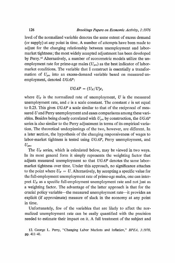
level of the normalized variable denotes the same extent of excess demand (or supply) at any point in time. A number of attempts have been made to adjust for the changing relationship between unemployment and labor- market tightness; the most widely accepted adjustment has been developed by Perry."2 Alternatively, a number of econometric models utilize the un- employment rate for prime-age males (Upm) as the best indicator of labor- market conditions. The variable that I construct is essentially a transfor- mation of Upm into an excess-demand variable based on measured un- employment, denoted UGAP:
UGAP = (UN/U)c,
where UN is the normalized rate of unemployment, U is the measured unemployment rate, and c is a scale constant. The constant c is set equal to 0.25. This gives UGAP a scale similar to that of the reciprocal of mea- sured U and Perry unemployment and eases comparisons among these vari- ables. Besides being closely correlated with U, by construction, the UGAP series is also similar to the Perry adjustment in terms of its empirical varia- tion. The theoretical underpinnings of the two, however, are different. In a later section, the hypothesis of the changing responsiveness of wages to labor-market tightness is tested using UGAP, Perry unemployment, and upm.
The UN series, which is calculated below, may be viewed in two ways. In its most general form it simply represents the weighting factor that adjusts measured unemployment so that UGAP denotes the same labor- market tightness over time. Under this approach, no significance attaches to the point where UN = U. Alternatively, by accepting a specific value for the full-employment unemployment rate of prime-age males, one can inter- pret UN as a specific full-employment unemployment rate and not just as a weighting factor. The advantage of the latter approach is that for the crucial policy variable-the measured unemployment rate-it provides an explicit (if approximate) measure of slack in the economy at any point in time.
Unfortunately, few of the variables that are likely to affect the nor- malized unemployment rate can be easily quantified with the precision needed to estimate their impact on it. A full treatment of the subject and
12. George L. Perry, "Changing Labor Markets and Inflation," BPEA, 3:1970, pp. 411-41.
Michael L. Wachter 127
of the difficulties of measurement and estimation requires a separate paper. Hence the UN measure of this paper is a crude proxy."3
Perhaps the most significant factor in changes in UN is the alteration in the age-sex composition of the labor force. Perry-and, more recently, R. A. Gordon, and Holt and his associates-have studied the importance of these demographic shifts. They have indicated that age-sex demographic shifts in the labor force heavily outweigh industrial, occupational, or geo- graphical shifts in affecting the impact of any given level of unemployment. Beginning with Perry, the measured unemployment rate has been replaced by a weighted unemployment rate to reflect this demographic shift.14
Second, and closely related to the demographic shift analyzed by Perry, the very sharp swing in the population and labor force toward younger workers, especially younger women, may have induced a supply-demand imbalance and a resulting relative increase in the unemployment experience of entrants into the labor market."5
According to this hypothesis, one can distinguish older workers with continuous labor-market attachment from younger workers and workers with discontinuous attachment in terms of their specific training. These labor groups become imperfect substitutes for one another so that the relative abundance of one group should alter wage differentials. If wage differentials among demographic groups are not sufficiently flexible, un- employment rates will change as well (or instead). In fact, in a world in which the labor requirements for capital equipment and the like are
13. The UN equation that I would have liked to estimate is of the form
(6) UN = g(A, CU, woa),
where A is the age structure of the population, Cu is the cost of being unemployed, and wa is the secular dispersion in the wage index. The discussion in this paper does utilize A and, to a much lesser extent, C.. The w, variable is omitted entirely. Data problems complicate the measurement of C. and wa, as theoretical problems do the definition of the proper independent variables. Attention must also focus on the relation- ship between the level of UGAP in the labor market and unutiized capacity in the goods market.
14. Perry, "Changing Labor Markets"; R. A. Gordon, "Some Macroeconomic Aspects of Manpower Policy," in Lloyd Ulman, ed., Manpower Programs in the Policy Mix (Johns Hopkins University Press, 1973); and Charles C. Holt and others, "Man- power Policies to Reduce Inflation and Unemployment," in ibid.
15. This type of "long swings" model is developed most fully by Richard A. Easterlin, Population, Labor Force, and Long Swings in Economic Growth: The American Experience (Columbia University Press for the National Bureau of Economic Research, 1968). See also Michael L. Wachter, "A Labor Supply Model for Secondary Workers," Review of Economics and Statistics, vol. 54 (May 1972), pp. 141-51.

128 Brookings Papers on Economic Activity, 1:1976
largely fixed, it may be difficult for relative wages to clear the market. And since young workers have a tendency to age over time, firms must anticipate demographic swings in the labor force. Of special importance in preventing relative wages from adjusting, and hence in thrusting the adjustment process onto unemployment rates, however, has been govern- ment policy. First, the major extension of minimum wages has prevented adjustments in demand that would favor lower-skilled workers. Second, changes in unemployment compensation and welfare have steadily in- creased the relative reservation price of labor, thereby lowering the cost of being unemployed.
Unfortunately, time series on the various transfer payments and mini- mum-wage laws that encompass both dollars per claimant and coverage are difficult to construct. Consequently, for this paper I cannot directly test the hypotheses-advanced by Feldstein and Ehrenberg and Oaxaca for unemployment compensation, Mincer and Welch for minimum wages, and Doeringer and Piore for welfare-that increases in the benefits avail- able and especially in the coverage of these programs have increased what I refer to as UN."6
The increase in coverage is of special importance since it largely affects the low-skilled workers who are disproportionately involved in cyclical unemployment and in the high turnover rates of the young and of (married) females. Reductions in the cost of being unemployed facilitate movements into and out of employment. Whether he is eligible for certain transfer payments helps an individual to choose between being unemployed and withdrawing from the labor force. The literature on unemployment com- pensation, minimum wages, and welfare, although not specifically related to UN, finds a displacement effect due to transfer payments that would have raised that rate significantly since 1962.
Thus, the demographic swing, coupled with the decline in the cost of un- employment, has operated to increase UN in two ways. First, these factors have caused a relative increase in the size of labor-force groups that his- torically display high UN. Second, they have increased structural and
16. Martin S. Feldstein, Lowering the Permanent Rate of Uniemployment, A Study Pre- pared for the Joint Economic Committee, 93:1 (Government Printing Office, 1973); Ronald G. Ehrenberg and Ronald L. Oaxaca, "Unemployment Insurance, Duration of Unemployment, and Subsequent Wage Gain" (Cornell University, August 1975; pro- cessed); Jacob Mincer, "Unemployment Effects of Minimum Wages" (Columbia Uni- versity, September 1975; processed); Finis Welch, "Minimum Wage Legislation in the United States," Economic Inquiry, vol. 12 (September 1974), pp. 285-318; and Peter B. Doeringer and Michael J. Piore, Internial Labor Markets and Manpower Anialysis (Heath, 1971).

Michael L. Wachter 129
frictional unemployment among secondary workers, thereby pushing up their already high Uv. Thus, the labor force is growing disproportionately in those demographic groups that have high and rising Uv, and this means a rise in the economy-wide UN.
A basic maintained assumption in calculating Uv is that UNPM, the UN of males in the prime-age group from 25 to 54, is largely unaffected by the labor-market developments that have altered UN. More specifically, UNpm is assumed to be constant at 2.9 percent. The justification for the constant level of UNPM is that the relative decline in the cost of being unemployed was due largely to increases in coverage rates for minimum wages and unemployment compensation and benefit levels for public assis- tance, alterations that affected prime-age males comparatively little. If they had an effect, they would have pushed UNPM up somewhat. Offsetting this factor, however, was the growing relative scarcity of this group in the labor force after 1962, which would have operated to decrease UNPM. As is well accepted, a benchmark or full-employment value for any adjusted unem- ployment rate is difficult to calculate with accuracy. My argument is that if the UN for prime-age males is the most stable, it is best to use that group's rate for a fixed benchmark rate. The 2.9 percent figure can be justified in a number of ways. For example, the work by Modigliani and Papademos supports this choice.'7 In the years that they identified as close to the "noninflationary rate of unemployment" Up,m averaged 3.03 percent; only one had a Up,, below 2.9 percent. Since 1954, Upm has been below 2.9 percent during 1956:2-1957:2, 1965:2-1970:2, and 1972:4-1974:3.
A popular technique for uncovering the noninflationary unemployment rate is to solve the Phillips curve. Using U, as the labor-market variable and estimating an equation of the form
(7) Wt = ao + E fplUt_, + E i=O ~~~i=4
results in -yYi > 1, so that UNPM is not defined. To calculate the lag structure on U, one is forced to constrain 1Yi = 1 and estimate the equation as a type of second difference in which the dependent variable is the rate of wage acceleration or deceleration; that is,
n m (7') t - 57 t-i = to + E gi ut-i
i-1 ieO
The resulting estimate of UATPM is 3.2 Dercent. 17. Franco Modigliani and Lucas Papademos, "Targets for Monetary Policy in the
Coming Year," BPEA, 1:1975, pp. 141-63.

130 Brookings Papers on Economic Activity, 1:1976
Besides requiring that the wage equation be perfectly accelerationist- that is, that Dyj = 1-an additional problem with this approach is that the noninflationary rate is calculated as the ratio of two parameters from the statistical, unstable Phillips curve. These considerations limit the use- fulness of a noninflationary unemployment rate or series constructed in this manner.'8
Since the normalized unemployment rate is based on labor-market hypotheses that are exogenous to the Phillips curve, the UN concept adopted here should be distinguished from the value of the unemployment rate, determined by the parameters of the unstable Phillips curve, which implies a nonaccelerating inflation rate at any given point in time.
The particular value assigned to UNPM has little effect on the Phillips- curve equations estimated in the next section. Changing this value would alter the mean of UGAP, but would do little to the variance (around the mean) of the series, or, as a consequence, to the regression results of the next section.'9
To calculate UN I first estimated
(8) In (Uj) = ao + a, In (U,) + a2ln (RP,),
where U, is the unemployment rate among prime-age males, 25 to 54 years of age; Ui is the age-sex unemployment rate, and RP, is the population of individuals 16 to 24, relative to the total population of working age. 20 The equation estimates for the period 1948-75 are presented in table 3.
18. The variance of UNPM is infinite since it is the ratio of two normally distributed variables. The variance can be approximated, but this term is very large so that the confidence interval around UNPM encompasses values that are outside the observed range of any unemployment rates. Hence, it is not possible to choose "conservative" values for UNPM that lie within a standard error of the coefficient. More generally, the noninflationary unemployment rate is a statistic that should be calculated from a model that includes at least all of the equations with feedbacks among wage changes, price inflation, and unemployment. This is beyond the scope of this paper.
19. Ross and Wachter, "Wage Determination," discusses the possibility that UN may increase as a function of the inflation rate. If this is the case, the results of the following section still hold, but the implications for stabilization policy are very different.
20. The use of relative population rather than relative labor force as an explanatory variable is based on the strong endogeneity of the latter. Besides the effects of money illusion discussed earlier, Easterlin, Population, Labor Force, and Wachter, "Labor Supply Model," argue that real-wage or standard-of-living effects may also be arguments in the labor-supply model. These operate through relative population swings as the exogenous variable. Hence, in this framework the RP, variable is the correct indepen- dent variable that causes changes in labor-force participation rates. In a structural version of equation 8, the relative wage term should be used in place of RP,.

Michael L. Wachter 131
Table 3. Results of Logarithmic Regression of Unemployment Rates for Various Demographic Groups on Unemployment Rate of Prime-Age Males and Ratio of Population Aged 16-24 to Total Population of Working Agea
Population Prime-age 16-24 years
male of age relative unemployment to total Durbin-
rate population Watson Sex and Constant Up. RPy? A2 statistic
age group (1) (2) (3) (4) (5)
Male 16-19 5.0547 0.6011 1.3670 0.7346 1.25
(17.39) (16.51) (10.39) 20-24 3.1200 0.9335 0.9354 0.8704 0.79
(11.18) (26.72) (7.41)
25-34 1.4517 1.0798 0.6150 0.9804 1.33 (12.03) (71.48) (11.26)
35-44 -0.3497 0.9969 -0.1090 0.9823 1.58 (3.13) (71.27) (2.16)
45-54 -1.4497 0.9142 -0.6515 0.9765 1.54 (11.40) (57.41) (11.32)
55-64 -1.3285 0.8218 -0.7110 0.9037 1.07 (5.41) (26.73) (6.40)
65 and over 0.4121 0.6375 -0.0775 0.7221 1.39 (1.24) (15.39) (0.52)
Female 16-19 6.5012 0.3831 1.9038 0.4575 1.34
(13.64) (6.42) (8.83)
20-24 5.0420 0.5674 1.6089 0.6726 0.92 (14.99) (13.48) (10.58)
25-34 3.3319 0.5451 0.9668 0.6989 1.19 (11.93) (15.60) (7.65)
35-44 2.5699 0.5745 0.7586 0.7014 1.00 (8.88) (15.84) (5.79)
45-54 1.2669 0.5756 0.2747 0.7446 1.19 (4.73) (17.18) (2.27)
55-64 -0.2180 0.5374 -0.3512 0.6867 1.19 (0.67) (13.28) (2.40)
65 and over 3.1828 0.5452 1.1798 0.4375 1.46 (6.45) (8.83) (5.29)
Source: See text equation 8 for logarithmic functional form. a. The numbers in parentheses are t-statistics.

132 Brookings Papers on Economic Activity, 1:1976
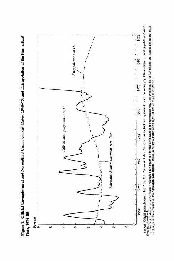
Assuming that UNPM is unchanged, the estimated values in columns 2 and 3 lead to normalized rates for each of the Ui. The coefficient for the population aged 16 to 24 relative to the total population then indi- cates the time-series changes in the UN for each group resulting from the demographic imbalances in the labor force. Aggregating the group UN at each point in time using actual labor-force weights results in the overall UN series depicted in figure 1.21
Taking RP, as an indicator of demographic imbalance for all groups in the labor market is not a strong assumption. Demographic trends being what they are, a relative increase in young people in the population implies quite directly a decrease in the relative population of older people. The equation then identifies which demographic groups are substitutes for younger workers (a2 in equation 8 > 0) and which groups are complements (a2 < 0). Essentially, almost all female groups and the young male groups have a2> 0, while the older male groups have a2 < 0.22
The UGAP series in its empirical variation, if not in its theoretical under- pinning, is similar to that originally calculated by Perry. To demonstrate the close relationships among the various unemployment measures-the UGAP construct, the unemployment rate for prime-age males upon which it is based, and the Perry-weighted unemployment measure, Up-I show their simple correlations below.23
UGAP Upm Up w UGAP 1.0000 Upm 0.9830 1.0000 Up 0.9731 0.9776 1.0000 wi 0.4678 0.3999 0.3224 1.0000
21. The weighted average of the separate unemployment rates calculated for men aged 25-34, 35-44, and 45-54, on the assumption of an overall rate for prime-age males of 2.9 percent, may deviate from that assumed 2.9 figure. In principle, an iter- ative procedure could have been used to ensure consistency. In practice, the inconsis- tency was small enough to be safely ignored.
22. A UN series was also constructed by regressing Ui on Upm and the relative popu- lation of each demographic group. Still another replaced RP, with a time trend broken in 1962 (when both demographic shifts and major increases in transfer payments began to occur). The results were largely unchanged.
23. It is also reassuring that most weighted unemployment measures that are similar to the Perry unemployment measure also suggest that the current noninflationary un- employment rate is approximately 5.5 percent. See, for example, Robert E. Hall, "The Process of Inflation in the Labor Market," BPEA, 2:1974, pp. 343-93; Modigliani and Papademos, "Targets for Monetary Policy," and George E. Johnson, "The Deter- mination of Wages in the Union and Nonunion Sectors" (University of Michigan, 1975; processed). The UGAP series, however, starts at a lower level and thus hlas climbed mnore rapidly during the 1960s and 1970s than has weighted unemployment.
0 *0 ci
00
P%~ ~ ~ ~ ~ ~~~~~~' 0
0
0
00
Z 0~~~~~~~~~~~~~~~~~~~~~~~~~~~~~~~~~~~~~~~~~~~~~~~~i 0
0 04
0 .~~~~~~~~~~~~~~~~~~~~~~~~~~0 0 00
" 0
o L. .~~~~~~~~~~~~~~~~~~~~~~~~~~~~~~~~~~~~~~~~~~~~~~~~o 0
0~~~~~~~~~~~~~~~~~~~~~~~~
>4.
0 to C's
- 1 0. 0~
.0 0
0.-
0
0.o0 ~o0 0l
P--4 cn~~~~~~~~~~~~~~>
0
Pll ck' 4. 00
4. 0

134 Brookings Papers on Economic Activity, 1:1976
The Aggregate Phillips Curve, 1954:1-1975:2
In testing for the changing responsiveness of wages, both structural and reduced-form wage equations are estimated. The relevant equations are 3 and 5 given above. To test for shifts in the slope of UGAP, a cross- product between UGAP and the log of time (UGAP * LT) is added. The type of time trend to be included is arbitrary in that no theory identifies a preferable one. The form adopted here is a log function that begins arbitrarily in 1945 and thus has an initial value of 4.92 (1954: 1) and a final value of 5.40 (1975:2). In fact, the log values over this range are close to a linear trend and a check of a few equations indicates no substan- tive difference in results between the alternative forms. Including the trend, equation 3, for example, can be rewritten as
m m n
(9) iWt = ao + E fjUGAPt_i + 3 j(UGAPt_i * LTt-i) + >2 -it-., i=O i=O i=l
where the term UGAP * LT introduces the maintained hypothesis that the coefficient on UGAP has changed monotonically over the estimation period (following the log trend). In this form, the total direct effect of UGAP on w can be calculated from
m m
5D /i3 + E 6iLTi.
The choice of the period for most of the equations, 1954: 1 through 1975:2, was dictated by the need for lagged observations on the independent variables.
As outlined above, any variant of equation 3 or 5 must have at least two components: a variable reflecting the tightness of labor markets is needed to measure movements along a Phillips curve, while the second component is needed to set the height of the Phillips curve. As stressed above, given the interaction between excess demand and inertia or expecta- tion variables, no set of independent variables can neatly divide the two; indeed, the second is essentially the long-lagged effect of the first. Conse- quently, the coefficient of one term will depend upon the specification of the other.
The wage equations, or Phillips curves, estimated here are, by hypoth- esis, assumed to have unstable parameters. Since these coefficients are time variant, the fitted equations are designed to describe the estimation

Michael L. Wachter 135
Table 4. Wage Coefficients of UGAP and the Nonfarm Deflator, Various Periods, Beginning 1954
a2 Percentage change in
a, prices a, Period UGAP p t-l I-a2
1954:1-1965:4 2.6689 0.1486 3.13 -1968:4 3.1126 0.1363 3.60 -1969:4 3.3106 0.1517 3.90 -1971:4 2.4692 0.4115 4.20 -1973:4 2.9981 0.3045 4.31 -1975:2 2.7292 0.3946 4.51
Source: Derived from equation wvt = a0 + alUGAPt + a2jt.1, where UGAP = (UN/U) times 0.25; U is the official unemployment rate, and UN is the normalized unemployment rate series given in figure 1; the definitions of the other sylmibols are as in table 1.
period. In general, I relied on the R2, t-statistic for individual coefficients, and F test for groupings of variables to choose the equations that tell the best story of the past two decades. Ability to predict the future is ignored, not only because all of the available observations are used in the estima- tion period, but also because of uncertainty about specifying the time- varying coefficients that guide the unstable tradeoff through time.
SEQUENTIAL ESTIMATES OF A SIMPLE PHILLIPS CURVE
The first test of changing responsiveness is to reestimate the equation of table 1, replacing official unemployment with UGAP. This substitution in- dicates how much of the decline in the slope of that Phillips curve is due simply to the inability of the official unemployment rate to reflect labor- market conditions because the nature of unemployment has changed. The results show that the decline in the slope of the Phillips curve, indicated by the changes in the coefficient a,, disappears when UGAP replaces U- (see table 4). In contrast with the sharp decline in the coefficient on U-1 in table 1 after 1970, the coefficient on UGAP is mostly stable over this period.24 Hence, failure to take account of the changing nature of unem-
24. In more complicated equations with several price variables and constructs such as "hidden unemployment," it seems to make less difference whether UGAP or U is used. The reason is that the UGAP and UN effects are partially absorbed into these additional labor-market and autoregressive terms. See, for example, Robert J. Gordon, "Wage-Price Controls and the Shifting Phillips Curve," BPEA, 2:1972, pp. 385-421. The additional variables in these more complicated structural equations, however, are themselves often constructed from the basic variables that appear in equations 3 and 5.
136 Brookings Papers on Economic Activity, 1:1976
ployment can lead to the presumption that wage inflation responds less to excess-demand pressures today than in the past. The tilt in the Phillips curve toward the horizontal disappears when the unemployment variable is adjusted for changes in UN.
Analysis of the increasing values of the price term in table 4 suggests an even stronger conclusion. The feedback effect grows in importance and it contributes to the long-run or total influence of UGAP on wage inflation. That total effect is given by the formula all(1 - a2) which has been growing continuously since 1965, as the last column of table 4 demonstrates.
THE UGAP COEFFICIENT: CHANGES OVER TIME
Next, I shall estimate a number of alternative Phillips curves to test directly for a changing coefficient on UGAP. The purpose is not to locate the best fit, but rather to indicate the robustness of the finding on the changing slope of the Phillips curve. In all cases, the coefficients on UGAP and UGAP * LT indicate an increasing slope for the Phillips curve over the years 1954-75. Since the intercept is held constant, the increasing coefficient on UGAP not only increases the slope of the Phillips curve but also pivots the curve outward.25
Equation 5.1 in table 5 improves on the equations of table 4 by adding the cross-product UGAP * LT but omitting any lags. Even from this simple form the basic finding emerges: the Phillips curve is getting steeper. In this and in all other equations, the negative sign on UGAP does not indi- cate a perverse slope for the Phillips curve. That negative value serves as a constant drag on the size of the combined or full UGAP coefficient. Since LT increases with time, the positive sign on UGAP * LT means that the full coefficient is growing. In addition, the combined coefficient, 2/3i + Z2ysLT, is always positive within the estimation period; that is, even when LT is at its lowest value, yALT > 10j. The t-statistics on UGAP and UGAP * LT in table 5 relate to the statistical significance of intro- ducing the respective terms, and their size is related only indirectly to the important matter of the significance of the combined coefficient. The stan- dard error of the full coefficient is given by
Vofgn + Lf2a + 2LThzp;z7-
25. An 'attempt to separate empirically these two factors-the outward shift of the Phillips relationship and its changing slope-is discussed below.

10 0
- ^ 0o 0 00 ti ^ ^ CUo 0
C~~~ C) 00 "Zt m en ~ ~ ~ 0 C)
Cf N-i ~ N- e f N- N N-** C) 0. 0
000~~~00 000 0 . 1
1.0 r- r- r- r- ~ 0
C.0 0
* . ~~~ ~~~~~~~00 c-IC
o b o o m *
O O O : O O O O O O g V.C)7
1W1 ~ ~ ~ C 0 oo Ia E ? C; ~~~~C)C C)
te) ~~~~~~~~~~0
* C )- .. .
oo C) C)
. . . . C)~-
* N -O * 00
* 0
ON cn Zt 00 00 x~~~~~~~~00 Cr
*0
'C * *E * . ...C
. . . . tn , * t 4 * ?? , ? * 0 -
If) . I; * * * * 0 * 'mCr . * O . _ ~ 0
_z~~~~~~~~~~~f0 c-_ _v .7o j-t4 A
aC)
*N N rII I
1 00 'IO oo CW oo CD oN ? 0o ?
O
O W b b O t s W o m o0 C)b tD B ,5
0 ~
- CI~000~000~00~0N- * t* 00 en "o .o 0 o
0 b t 000 '--C ^ U bi C c- O 04
-. ~~~~~~~~~~~~~~~~~~~~~~0~
> ; t > < O 6) :) o -4 t tn o < W -
, (>
00~~~~~~~~~0 0~'
C 0N 0C-.0 . Cf0 C -i 0 0
;;~~~d .c-. ~ 0 0 ---, C0aaa
:J0 0~~~~
.2 o, *
o 0 , =
-~ CI-0C~CI~-000N- 00 CfCf 0-0 v . ~~ e~n00~-4C~1'-4 0 - - 0- . 00
42 IZ "I @t C) C) I' IN t 3 tn 11 tn Ct en V s. a;. O Cl N- ci - CI CC - 00 ON N ZT N N N N e ? Cn 0 tf _
0 C ? 0 0 0
V 0 0C)CUCo0 C
* .O & N Z 0
Q Cr m m m m m m m m m m #aLoRSt O#e~~~> C1 t3 21 ens 0 42e e _
zi ~ ~ ~ ~ ~ ~ ~ OC
t:v te)~ ~~ II~Ii

138 Brookings Papers on Economic Activity, 1:1976
The resulting t-statistics are found to be highly significant, with values generally above 3.
Equation 5.2 retains the UGAP term without lags and introduces a six-year (to completion) lag on prices. The UGAP term exhibits the in- creasing coefficient over time; the combined coefficient is 2.64 at the be- ginning of the estimation period and 3.69 at the end (see table 6), and it is significant, with t-values that range from 3.73 to 7.52. The coefficient on the price term is close to unity. One cannot analyze the long-run Phillips curve, however, without access to other equations. In any case, comparing equations 5.1 and 5.2 makes clear that introducing a lag on prices con- siderably strengthens the implied feedback or indirect effect in this single equation.
Equation 5.3 omits the cross-product UGAP term but includes lags on both UGAP and pl. This standard Phillips curve, defined on UGAP with constant coefficients, is introduced for purposes of comparison, so that the effect of adding the UGAP * LT terms can be evaluated more easily.
Equation 5.4 includes the various lags and the interaction term UGAP * LT. The combined coefficient ranges from 2.87 in 1954 to 4.41 in 1975 (table 6). Several interesting results appear in this equation. First, the ,j3 add up to (a maximum of) 4.41 after three years. In equation 5.2, in which the UGAP terms had no lags, the maximum value of the coefficient is 3.69. Hence, introducing a lag adds only a small amount to the direct effect of UGAP on wv, but spreads it out over several years. The short-run responsiveness of inflation to unemployment is greater in equation 5.2 than in 5.4. Also, the long-run coefficient on pl falls below unity in 5.4 (see table 5). The change is, however, scarcely more than one standard error, so little should be made of this difference.
Equation 5.5 is a recalculation of 5.4 with the reciprocal of Perry unem- ployment replacing UGAP. The substitution confirms the basic results. The increasing slope of the Phillips curve again appears, with the coefficient rising from (approximately) 2 to 4 over the estimation period (table 6). The lagged price term is back to unity and the fit of the equation is largely unchanged. The same equation was also run using unemployment of prime- age males and its cross-product term in place of Perry unemployment. The results showed the same pattern as that observed for Perry and UGAP unemployment, so they are not reproduced here.
Two different methods are applied to capture the inertia or expectation

Michael L. Wachter 139
Table 6. Values of Combined UGAP Coefficient, Representative Equations fronm Table 5, 1954:1 and 1975:2
Coefficient
Beginning End of of estimation estimation
Equation period, 1954:1 period, 1975:2
5.2 2.64 3.69 5.3a 3.23 3.23 5.4 2.87 4.41 5.5 1.96 3.87 5.7 1.38 3.09 5.9 2.65 4.52
Sources: Derived from combined UGAP coefficient, 2;pi + 2;-yiLT (where UGAP is as defined in table 5), and equations 5.2-5.5, 5.7, and 5.9 in table 5.
a. Since this equation omits the DyiLT term, the coefficient is unchanged from the UGAP coefficient for equation 5.3 in table 5.
effects. Equations 5.2 through 5.5 use a distributed lag on past price changes (the nonfarm deflator), currently the most popular method of capturing these lagged effects. The results of these structural equations are accelerationist in tone (although with a very long lag) as the coefficient on p1 is close to unity. The lag on p1 is a fourth-degree polynomial, spread over twenty-four quarters and not constrained to zero at either end be- cause such a lag is best able to capture the possibility that the lag structure may well be greater than twenty-four quarters. The mean lag is approxi- mately ten quarters and varies little across these equations.
USE OF MONEY AS A LAGGED VARIABLE
To establish more directly the role of excess demand in the inertia- expectation process, the rate of change in the money supply lagged one period (denoted rm and representing currency plus demand deposits) is introduced into the wage equation. As is the case in the equations in which prices are the independent variable, the change in the money supply is entered with a one-period lag and with a twenty-four-quarter Almon lag (fourth-degree polynomial with the lag unconstrained at either end). Comparing the equations 5.6 and 5.7 with mhl and those with p1 indicates that the quasi-reduced-form demand approach does as well as the auto- regressive structural equation (using price inflation). The Rf2 and individual parameter fits are largely unchanged. The coefficient on mi7l is, on average,

140 Brookings Papers on Economic Activity, 1:1976
somewhat lower than the coefficient on p1, but reasonably simple altera- tions in the structure of the equation can also bring this coefficient within a standard error of unity.2"
The success of replacing p1 with mhI is particularly impressive because the autoregressive features in p1 are likely to improve the fit of the equa- tion (without necessarily adding any economic explanatory power). Fur- thermore, equations containing mhl have strong implications for the role of aggregate demand in the wage-inflation process. The traditional lagged price and wage measures have often been interpreted as reflecting forces other than demand. The money supply, on the other hand, is plainly a demand variable.
The Phillips-curve equations containing UGAP and mhl imply a strongly neoclassical view of the wage-inflation process: a short disequilibrium effect, related to the size of UGAP, and a longer-run steady-state influence from growth in the money supply. The long lags in rhl-over two years to 50 percent adjustment-are not unexpected if one adopts the kind of argu- ment relying on institutional rigidity discussed earlier.
EFFECT OF CONTROLS
Because the period after 1970 is of special interest, the role of the con- trols program established by the Nixon administration in 1971 is of some importance. To the extent that the policy altered the time path of wage inflation, its exclusion could bias the results, especially since the time- varying coefficient on UGAP is largest in the past few years. The problem with any controls program lies in quantifying a variable to measure its impact.27 The best solution is to adopt an a priori hypothesis. My own view is that the controls had no long-run effect. Rather, they slowed wage inflation during Phases I and II and then were neutral during Phases III and IV, but did not permit a wage catch-up. At their termination, the suppressed wage inflation was released, and by 1975 the wage level was restored to what it would have been had controls not been implemented (with all other independent variables following their actual time paths).
26. The smaller indirect effect resulting from the below-unity coefficient on m1l may be related to the issue of the appropriate money-supply measure for inflation equations. That problem is beyond the scope of this paper.
27. See Walter Oi, "On Measuring the Impact of Wage-Price Controls: A Critical Appraisal" (University of Rochester, February 1974; processed).

Michael L. Wachter 141
This development is built into the variable NIXCON, which appears in equations 5.8 and 5.9.28
The NIXCON variable does not change the overall results, and it is only marginally significant. The combined coefficients on the labor-market variables are raised somewhat, comparing equation 5.4 with 5.8, and 5.5 with 5.9. To check further the meaning that the controls program might have for the validity of the central hypothesis of an increasing slope on the Phillips curve, equation 5.10 is estimated ending in 1971:2, before the im- plementation of controls. The negative sign on UGAP and the positive sign on UGAP * LT again signify an increasing coefficient over time for the combined coefficient. As in all the other equations, the range of the co- efficient is positive and statistically significant over the estimation period.
I attempted to control for "exogenous" wage and price developments by allowing the constant to shift over time. In particular, this maneuver was aimed at capturing developments such as the increases in oil prices in 1973-74. These equations do not alter any of the main conclusions of this study, and they are not reproduced here. Including the wage or price change in a specific industry to capture "exogenous" inflation presents a problem, because only rarely are these developments genuinely independent of demand in an economy as large as the United States. Including them in the equation, however, dilutes the impact of the demand variables that are likely to be affecting both industry and aggregate rates of wage change.29
THE EXPECTATION COEFFICIENT: CHANGES OVER TIME
It is difficult to test for an upward shift in the parameter of the money- supply variable or price variable, as well as the increasing slope of the Phillips relationship. The two phenomena are probably, though not neces-
28. I did not experiment with specifications for the NIXCON variables. However, my a priori specification did benefit from previous studies on the controls program. The relevant issues and literature are summarized in Michael L. Wachter, "The Wage Process: An Analysis of the Early 1970s," BPEA, 2:1974, pp. 507-24. See also Robert J. Gordon, "The Response of Wages and Prices to the First Two Years of Controls," BPEA, 3:1973, pp. 765-78.
29. Furthermore, there must be some notion that the cost-push pressures from prob- lem sectors are ongoing. For example, whereas the initial rise in oil prices was due, at least in part, to broadened monopoly power, further rises should not be labeled exoge- nous or cost-push unless the relative price continues to increase. For a counterexample in which structural problems cause ongoing sectoral inflation, see Susan M. Wachter, Latin American Inflation (Lexington Books, 1976).

142 Brookings Papers on Economic Activity, 1:1976
sarily, related. In the model sketched above, wage inflation is ultimately due to excess-demand pressures. Short-run labor-market effects are mea- sured by UGAP. Longer-run, inertia or expectation factors are captured either by pl or ml 1. One can interpret these variables as the far end of the excess-demand lag. Hence, an increasing coefficient on p1 or 'mI argues that the longer-term effects are becoming more important, whereas an in- creasing coefficient on UGAP strengthens the short-run adjustment of the Phillips curve.
The strategy of including time-varying parameters on both pl (or rm 1) and UGAP had mixed results. On the one hand, the results in most cases argued for increasing parameters on both variables. However, the degree of multicollinearity produced lag structures that are difficult to interpret in an economic sense and incorrect signs on some of the coefficients over much of the estimation period.
The final approach, using the 1954-75 data period, is to allow the param- eters to vary on mhl and p1 but not on UGAP. Here again, the inertia or expectation coefficient shifts upward. An attempt to ascertain whether in- cluding a cross-product on mhl or p1 but not on UGAP would do better than the reverse specification proved futile; one specification did not clearly dominate the other. That the coefficient on p1 has been increasing over the postwar period comes as no surprise. Gordon, for example, substituted a nonlinear price-expectations term that, given the performance of inflation over the past decade, is not dissimilar to a time-trend interaction variable. Although Gordon did not deal with the issue of increasing responsiveness, his finding that the coefficient on p1 increases with the rate of inflation is relevant. In this case, the increased responsiveness arises through the feed- back effect and suggests a longer mean lag as well as a larger long-run value for the full coefficient. Similar results can be obtained by substi- tuting hl for pl.8I
As mentioned above, whether or not the coefficient is increasing on UGAP or pl (or mhl) affects the mean length of the response. In all cases,
30. Robert J. Gordon, "Wage-Price Controls and the Shifting Phillips Curve," BPEA, 2:1972, pp. 404-06. Of course, nonlinear formation of expectations or any other scheme that uses either fixed weights or functional forms to allow coefficients to vary is open to the rational-expectations critique. Presumably, economic actors will eventually learn the systematic component of any policy strategy, hence foiling future forecasting efforts. My choice of a time-varying coefficient on UGAP is designed to test the hypoth- esis, suggested by a number of observations (mentioned in the first section), that the coefficient varied more or less monotonically over the postwar period. It does not suggest that this time path is likely to continue.

Michael L. Wachter 143
the eventual response to aggregate demand is stronger. In my equations, which stress the increase in the UGAP full coefficient, it is the short-run response that is strengthened.
Viewing the Shift
As discussed earlier, the regressions in table 5 have a (time-varying) cross-product term only on the UGAP or Up variable. This forces the short-run Phillips curve to shift outward as it becomes steeper. To present a clearer picture of the change between the 1954 and the 1975 Phillips curves, I have added a trend term to the constant in addition to the UGAP * LT term. This allows the Phillips curve the latitude to become steeper without shifting outward, or to contradict the earlier results by shifting outward and becoming flatter. The extra trend variable, of course, increases the collinearity among the independent variables; statistically, it is difficult to discriminate among these various hypotheses. As a conse- quence it should not be surprising that the shift in the slope was not sig- nificant at traditional levels of confidence for some equations (including those shown below), although it was for others. Adding a shifting trend term to the constant in equation 5.2 results in wage equations for 1954 and 1975, respectively, of the form
(10a) 1954: iw = -0.0809 + 2.0680 UGAP + 1.0073 pI; (0.25) (1.04) (7.64)
(lOb) 1975: iw = -0.2963 + 4.0490 UGAP + 1.0073p1. (1.45) (2.59) (7.64)
Making the same addition to equation 5.5 yields
(lla) 1954: iw = 0.1839 + 1.9148 Up-' + 1.0992pl; (0.55) (1.10) (7.88)
(lIlb) 1975: iw = 0.2084 + 3.3997 Up-i + 1.0992P1. (0.68) (2.23) (7.88)
The short-run Phillips curves derived from these equations, by setting pl = 0, are shown in figures 2a and 2b, respectively. The diagrammatic approach helps to show the combined impact on the wage equation re- sulting from the changing size of the coefficients on UGAP (recorded in table 6) and the constant term, and the increasing level of UN. In a com- parison of the curves for 1954 and 1975, each at its respective UN, the

2
Ec to cl
00
Cu~~~~~~~~~~~~~~~~~~~~~~~~~~~~~~~~~~~~~~~~~~~~~~C
0~~~~~~~~~~~~~~~~~
~~~~~~~ 0 ~~~~~~~~~~~~~~~~~~~~~u0
o 00o 0X
t Xo cfi Xb?ut^No!
0
Cu~~~~~~~~~~~~~~~~~~~~~~~~~~~~~~~~~~~~ac >
- ~~~~~~~~~~~~~~~~~~~~~~~~~~~~~~~~~~~~~~~~~~~~~~~~~~~~~~~~~~4 0~~~~~~~~~~~~~~~~~~~~~~~
00
P-4 0 rA~~~~N
00~~~~~~~~~~~~~~~~~~
Michael L. Wachter 145
1975 curve has a steeper slope, but by a smaller margin than that implied by table 6. Both the decreasing size of the constant term and the increasing coefficient on UGAP contribute to a steepening of the short-run Phillips curve. On the other hand, it is obvious that at a given low level of unem- ployment-say, 3 or 4 percent-the steepening is dramatic. Most impor- tant, the very steep portion of the nonlinear Phillips curve is now in the unemployment range relevant for policy.
The labor-market term with Perry-weighted unemployment (Up) is plotted by assuming a transformation (suggested by George Perry) into U space of Up = U - U + Up, where the bars indicate average values of the rates (calculated separately for the mid-1950s and 1970s). The Phillips curve based on Up is also steeper in 1975 than in 1954. In fact, the increase in the slope over time is greater in the Up than in the UGAP equation. Here again, the dilemma posed by the nonlinearity in Up (or UGAP) is indicated. A rise of U of several percentage points above UN still buys only moderate deceleration of inflation; while for U lower than UN, unemploy- ment rates as high as 4 percent now spur sharply accelerating rates of inflation.
To illustrate the message of these equations for the current wage re- sponse to UGAP, I have traced through a hypothetical example using equa- tion 10b. This example is meant solely to illustrate the potential impact of changes in unemployment on inflation; it is not a forecast of a simulated wage equation. The numbers in the example assume that the system starts from equilibrium, free of any heritage effects. The calculations assume that price changes follow wage changes with a unitary coefficient and with no lag. Although this assumption imparts an upward bias to the speed of the wage response, I offset this effect somewhat by ignoring any direct de- mand effect operating through the price equation. In terms of equation 2, 42 = 1 and 4)3 = 0. The productivity term in the price equation is set equal to 2.8, which yields a stable Phillips curve (that is, the rate of inflation is stable when U = UN).
The results are shown in table 7. For example, suppose that U is main- tained at 8 percent with UN at 5.5. With the 1975 UGAP coefficients, wage inflation will decline from its initial rate by 1.7 percentage points by the end of the first year, 2.1 points in two years (that is, an additional 0.4 point in the second year), and 2.4 points in the third year. After six years, the total response will be approximately 4 points. Even if the recession is terminated earlier, the recession values for UGAP will become part of the

146 Brookings Papers on Economic Activity, 1:1976
Table 7. Hypothetical Examples Showing Effect of the Relation between the Official and the Normalized Unemployment Rates on Wage Acceleration and Deceleration, 1975a Change in rate of wage inflation, in percentage points
Value of official and normalized Year
unemployment Value of UGAP rates (percent) coefficient 1 2 3 4
Cumulative wage decleaation
U = 8 0.17 -1.68 -2.05 -2.37 -2.73 UN= 5.5
U = 6.5 0.21 -0.85 -1.04 -1.20 -1.39 UN = 5.5
Cumulative wage acceleration
U= 4 0.34 1.91 2.34 2.69 3.11 UN = 5.5
U= 3 0.46 4.29 5.26 6.06 7.00 UN = 5.5
Source: Derived from text equation lOb. a. Initial conditions are U UN and wve = Wt_, followed by a once-and-for-all change in the value of
UGAP as indicated, where the symbols are as defined in tables 1 and 4.
heritage in pl, causing downward pressure on wage inflation into the future.3' These longer-run heritage effects are especially important because the lag structure on p1 (or mhl) is very flat. This, in turn, implies an espe- cially long adjustment process between wv and UGAP.
These calculations are based on the unlikely assumption that the coeffi- cients of the wage equation remain unchanged over the period of high unemployment. If the increasing "inflationary bias" of the wage equation is due to the heritage of tightening labor markets over the postwar period, then persistently weak labor markets should yield some additional defla- tionary gains by altering the coefficients favorably.
31. Comparable calculations cannot easily be performed for the 1954 equation. Making them would require either setting the rate of productivity growth below 2 per- cent or assuming that the true noninflationary unemployment rate in 1954 was approxi- mately 3 percent. My UN estimate for 1954 is, on the other hand, close to 4 percent. If one redefines UGAP as c(UN!U), where UN is the 3 percent figure discussed above, then a recession comparable to the 1975 experience (with UGAP = 0.17) would require U = 4.41. In this case, the wage deceleration would be -0.86 after one year, -1.05 after two years, -1.21 after three years, and -1.40 after four years. As stressed above, however, the inflationary dynamics of the system depend on the full set of equations that contain wage-price-unemployment feedbacks.

Michael L. Wachter 147
Whereas these equations illustrate a slow, but persistent, moderation in wage inflation as a consequence of recession, the response to tight labor markets is quite different. Suppose that U is driven down to 4 percent while UN remains at 5.5 percent. As a consequence of the nonlinearity of the Phillips curve, the inflationary response is greater even though the hypo- thetical expansion gap is only 1.5 against 2.5 in the contraction example. Again on the basis of equation 5.2, wage inflation will be 1.91 percentage points higher in the first year and 2.69 points higher after three years (table 7). And, as mentioned above, even if the economy is cooled off so that U = UN, the period of U< UN will become part of the heritage and continue to lend impetus to wage inflation. If U is forced down to about 3 percent with UN at 5.5 percent, the first-year response alone will raise the rate of wage inflation by 4.3 percentage points; after four years the wage acceleration will be 7.0 percentage points. Hence, the wage equations estimated in table 5 indicate that unemployment rates similar to those observed during the late 1960s would cause a sharp acceleration in the rate of inflation.
The major finding of these regressions is that the unemployment terms, including their lagged effects, have an increasing coefficient over the period. In addition, both short- and intermediate-run Phillips curves (limited by the truncated unemployment series) have become steeper. This result is strikingly robust across the myriad forms of the wage equation, and holds whether the Phillips-curve term is defined to be UGAP, the unemployment rate for prime-age males, or the Perry weighted index. One important caveat: it is difficult to distinguish a shift in the Phillips-curve parameter from a shift in the inertia or expectation parameter. Both appear to have been increasing, but this development cannot be asserted with confidence.
The variables 61 and Ph 1 are viewed here as capturing the long-lagged demand influences working through an inertia or expectation mechanism. In particular, thepil term is interpreted as a kind of distributed-lag genera- tor of labor-market effects. Hence, the feedback from UGAP to wV to p (through the price equation) and then back to iv is an important compo- nent of the effects of aggregate-demand policies on the rate of wage infla- tion. On the other hand, mhl, entered into the quasi-reduced-form wage equation, represents a direct demand effect and replaces the feedback mechanism.32
32. This observation does not bear on the question of whether the money supply is passive in the sense of being determined by the rate of wage inflation. For evidence on

148 Brookings Papers on Economic Activity, 1:1976
Wage Behavior over the Business Cycle
In this section, rather than using a wage equation estimated over the 1954-75 period, I adopt a variant of the business-cycle methodology de- veloped by the National Bureau of Economic Research. This procedure allows a study of data disaggregated more finely and over a longer time frame and permits a direct comparison with the results previously reported by the Council of Economic Advisers and by Cagan.33 These studies showed, for wages and prices respectively, that the rate of deceleration around peaks has slowed markedly over the postwar years.
This analysis suffers from a timing problem: not all of the factors that determine wage inflation exert their maximum inflationary impact at a cyclical peak or their minimum effect at a trough. Of particular impor- tance is the influence of inflationary expectations or inertia. Given the long lags, the maximum impact of either p1 or mhl on wage inflation will gen- erally occur after cyclical turning points. And, given the quantitative sig- nificance of these variables, the resulting predicted wage series is likely also to trail NBER cyclical turns.34
UGAP CRITERION
The influence of lagged excess-demand factors suggests altering the dat- ing of turning points in wage inflation. Specifically, I date slack periods in the labor market from the time when U first rises above UN until the time when the two are again equal. This dividing line is meant to be sug- gestive and not to imply that the shift in the relation of U and UN is unique for changes in wage inflation. Clearly, the magnitude of the changes
this point, see Christopher A. Sims, "Money, Income, and Causality," American Eco- nomic Review, vol. 62 (September 1972), pp. 540-52, and Robert J. Barro, "Unantici- pated Money Growth and Unemployment in the United States" (University of Roch- ester, 1975; processed).
33. See table 2 above and Cagan, "Hydra-Headed Monster." 34. Although the NBER methodology has many useful points, it has some well-
known faults as well. A major issue is that cycles differ substantially in severity, making their distinctive features difficult to measure without a multivariate framework. To compound this problem, in attempting to analyze rates of deceleration of wage inflation around a peak, one is comparing the downturn relative to the previous expansion. Even if all downturns were the same (and, of course, they are not), the preceding expansions could be quite different from one another.

Michael L. Wachter 149
in UGAP and i1 or mhl is more central than any single dividing line. For example, lagged inertia or expectation effects may still be exerting upward pressure when U moves above UN. To measure the magnitude of the effects properly requires regression analysis.
Using the UN series presented in figure 1, this alternative dating scheme is shown below, along with the NBER series, in which P and T stand for peak and trough, respectively. The two schemes differ significantly in an- ticipating downward pressure on wage inflation.
NBER dating U Q UN dating
PtoT 1948:4-1949:4 U> UN 1949:1-1950:3 TtoP 1949:4-1953:3 U< UN 1950:4-1953:4 P to T 1953:3-1954:3 U> UN 1954:1-1955:2
U-- UN 1955:3-1957:3 Tto P 1954:3-1957:3 P toT 1957:3-1958:2 U> UN 1957:4-1965:1 T to P 1958:2-1960:2 P to T 1960:2-1961:1 T to P 1961:1-1969:4 U < UN 1965:2-1970:3 PtoT 1969:4-1970:4 U> UN 1970:4-1972:3 TtoP 1970:4-1973:4 U< UN 1972:4-1974:3 P to T 1973:4-1975:2 U> UN 1974:4-
DISAGGREGATED WAGE BEHAVIOR: AFTER WORLD WAR II
Table 8 presents the rate of wage change in high-, medium-, and low- wage industries for periods delineated by the UGAP criterion. The entries are all annualized rates of wage inflation dating from the beginning of the tight or slack period. Table 9 indicates rates of change the year before and the year after U crosses UN. The data strongly support the use of the excess-demand or UGAP criterion for dating reversals in wage pressure.
As shown in table 9, the UGAP criterion only twice misses the change- over in the rate of wage inflation over the postwar years. One miss, more- over, occurs in the midst of wage-price controls in 1972, making its meaning uncertain. The second occurs in 1970:3 when wv in the high- and medium- wage sectors continues to rise even though the economy has switched from a U below UN to U above UN; the low-wage sector has decelerating wage inflation as expected. (Indeed, the low-wage sector is on target even during the turning point influenced by 1972 controls.) It should be noted, how-
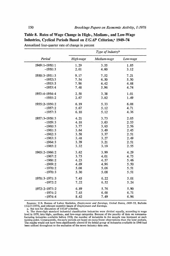
150 Brookings Papers on Economic Activity, 1:1976
Table 8. Rates of Wage Change in High-, Medium-, and Low-Wage Industries, Cyclical Periods Based on UGAP Criterion,a 1949-74 Annualized four-quarter rate of change in percent
Type of industryb
Period High-wage Medium-wage Low-wage
1949:1-1950:1 1.29 3.55 1.85 -1950:3 2.61 4.60 3.12
1950:3-1951:3 9.17 7.52 7.21 -1952:3 7.54 6.50 5.50 -1953:3 7.98 6.42 4.88 -1953:4 7.48 5.96 4.74
1953:4-1954:4 2.58 3.38 1.01 -1955:2 2.67 3.82 1.49
1955:2-1956:2 6.19 5.33 6.08 -1957:2 5.67 5.12 4.71 -1957:3 6.10 5.12 4.36
1957:3-1958:3 4.21 3.73 2.05 -1959:3 4.18 3.63 2.53 -1960:3 3.77 3.65 2.56 -1961:3 3.64 3.49 2.45 -1962:3 3.58 3.37 2.51 -1963:3 3.48 3.27 2.49 -1964:3 3.39 3.21 2.51 -1965:2 3.32 3.19 2.55
1965:2-1966:2 3.62 3.99 4.29 -1967:2 3.75 4.01 4.75 -1968:2 4.23 4.57 5.46 -1969:2 4.69 4.96 5.50 -1970:2 5.08 5.06 5.51 -1970:3 5.30 5.08 5.51
1970:3-1971:3 7.45 6.22 5.01 -1972:2 7.22 6.52 5.24
1972:2-1973:2 6.89 5.76 5.90 -1974:2 7.45 6.68 6.71 -1974:4 8.42 7.49 6.96
Sources: U.S. Bureau of Labor Statistics, Employment and Earnintgs, United States, 1909-72, Bulletin 1312-9 (1973), and relevant monthly issues of Employmenzt and Earnings.
a. See text for discussion of UGAP criterion. b. The three-digit standard industrial classification industries were divided equally, according to wage
level in 1970, into high-, medium-, and low-wage categories. Because of the paucity of data on nonmanu- facturing industries available before 1958, the number of industries in the sample was increased at each turning point. Consequently, the early periods are based on many fewer observations than the later periods. The results would not have been significantly altered if the initial group of industries available in 1948 had been utilized throughout to the exclusion of the newer industry data sets.

Michael L. Wachter 151
Table 9. Rates of Wage Change in High-, Medium-, and Low-Wage Industries, Year before and Year after U Crosses UN, 1949-72 Annualized four-quarter rate of change in percent
Turning point Type of industry
Date of Type changeover Period Highl-wage Medium-wage Low-wage
Downturn 1949:1 Year before 6.23 8.41 6.69 Year after 1.29 3.55 1.85
Upturn 1950:3 Year before 4.06 4.86 5.23 Year after 9.17 7.52 7.21
Downturn 1953:4 Year before 5.90 5.31 3.07 Year after 2.58 3.38 1.01
Upturn 1955:2 Year before 3.93 3.82 1.92 Year after 6.19 5.33 6.08
Downturn 1957:3 Year before 5.59 4.85 2.79 Year after 4.21 3.73 2.05
Upturn 1965:2 Year before 3.36 2.94 3.51 Year after 3.62 3.99 4.29
Downturn 1970:3 Year before 7.01 5.86 5.67 Year after 7.45 6.22 5.01
Upturn 1972:2 Year before 7.42 7.58 4.89 Year after 6.89 5.76 5.90
Source: Same as table 8.
ever, that this aberration occurred during by far the shallowest recession in the post-World War II years, as measured by UGAP. Furthermore, in the 1970 downturn, relative to past recessions, employment fell only slightly in the high-wage sector and scarcely at all in the medium- and low-wage sec- tors. The unemployment data for 1970 look much worse than either em- ployment or UGAP; that is, the upswing in unemployment was caused largely by an influx of young, relatively inexperienced workers, especially young female workers.35
The disaggregated data of table 8 exhibit several other interesting fea- tures. A lagged wage response is especially noticeable in the high-wage sector, less so in the medium-wage sector, and hardly at all in the low-wage
35. The minor nature of the downturn in 1970 is also found by analyzing the weighted unemployment series. This was first stressed by Hall, "Process of Inflation."

152 Brookings Papers on Economic Activity, 1:1976
sector.36 As would be expected, this slower pattern of response is especially visible in the longer periods of slack or excess demand. In these longer cycles, the lagged wage response (calculated at an annualized rate from the beginning of the period) is virtually always in the correct direction, even though the speed of adjustment may be slow. This pattern is particularly marked in the high-wage sector. Here, contractual agreements slow the response, but wages under new agreements are influenced by the new labor- market conditions, as well as by relative-wage considerations. The best evidence of this is the slow but persistent decline in the annualized wage change in the high-wage sector between 1957 and 1965 followed by the slow but persistent increase between 1965 and 1970 (see table 8). One can conclude that wage inflation changes direction according to the UGAP criterion and then continues to move in the direction predicted by the theory.
On the other hand, an inspection of tables 8 and 9 appears to suggest that the basic Cagan-CEA point still holds, but to a smaller extent than sug- gested in table 2: over the postwar period, in the first year after U crosses UN, the rate of wage deceleration or acceleration falls. A problem with concentrating on rates of deceleration, however, is that this second differ- ence is quite sensitive to the duration and magnitude of the upturn as well as of the downturn. For example, the 1950 expansion was greatly in- fluenced by the anticipatory, precontrols wage explosion of the Korean War, while the uptrend of the late 1960s was unique in its duration.
A very different, and, I believe, a more accurate picture emerges if one analyzes rates of inflation for the first year of tight and slack intervals. Do- ing so is especially useful for the period prior to 1970, when the Phillips curve was stable within a relatively narrow band. (The main reason Cagan looks at periods of deceleration is to correct for expectational shifts in the Phillips curve over time.) According to these results, the most significant aspect of the turning-point data before the 1970 recession is the tendency of wages to rise less rapidly in initial years of successive tight periods. For example, in the low-wage sector, the rates of wage change in the first year of the slack periods starting in 1949, 1953, and 1957 are 1.85, 1.01, and 2.05 percent, respectively, thus showing no clear pattern over time. For the subsequent tight periods, however, the wage inflation rates are 7.21, 6.08, and 4.29 percent, each less than its predecessor. A similar pattern appears
36. For further evidence, see Michael L. Wachter, "Cyclical Variation in the Inter- industry Wage Structure," American Economic Review, vol. 60 (March 1970), pp. 75-84.
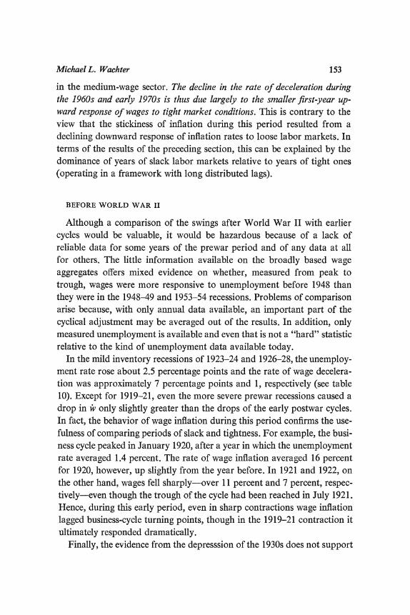
Michael L. Wachter 153
in the medium-wage sector. The decline in the rate of deceleration during the 1960s and early 1970s is thus due largely to the smaller first-year up- ward response of wages to tight market conditions. This is contrary to the view that the stickiness of inflation during this period resulted from a declining downward response of inflation rates to loose labor markets. In terms of the results of the preceding section, this can be explained by the dominance of years of slack labor markets relative to years of tight ones (operating in a framework with long distributed lags).
BEFORE WORLD WAR II
Although a comparison of the swings after World War II with earlier cycles would be valuable, it would be hazardous because of a lack of reliable data for some years of the prewar period and of any data at all for others. The little information available on the broadly based wage aggregates offers mixed evidence on whether, measured from peak to trough, wages were more responsive to unemployment before 1948 than they were in the 1948-49 and 1953-54 recessions. Problems of comparison arise because, with only annual data available, an important part of the cyclical adjustment may be averaged out of the results. In addition, only measured unemployment is available and even that is not a "hard" statistic relative to the kind of unemployment data available today.
In the mild inventory recessions of 1923-24 and 1926-28, the unemploy- ment rate rose about 2.5 percentage points and the rate of wage decelera- tion was approximately 7 percentage points and 1, respectively (see table 10). Except for 1919-21, even the more severe prewar recessions caused a drop in wv only slightly greater than the drops of the early postwar cycles. In fact, the behavior of wage inflation during this period confirms the use- fulness of comparing periods of slack and tightness. For example, the busi- ness cycle peaked in January 1920, after a year in which the unemployment rate averaged 1.4 percent. The rate of wage inflation averaged 16 percent for 1920, however, up slightly from the year before. In 1921 and 1922, on the other hand, wages fell sharply-over 11 percent and 7 percent, respec- tively-even though the trough of the cycle had been reached in July 1921. Hence, during this early period, even in sharp contractions wage inflation lagged business-cycle turning points, though in the 1919-21 contraction it ultimately responded dramatically.
Finally, the evidence from the depresssion of the 1930s does not support

Table 10. Rates of Wage Change in Manufacturing, Various Series, Pre-World War II Unemployment Cycles, 1902-38 Annual rate in percent
Wage series and coverage
BLS
Male Rees, All
Cyclea all manu- production Semi- All mann- and period facturingb workers Unskilled skilled facturing
1902-04 Year before peak
to peak 6.92 ... ... Peak to trough 1.32 ...
1906-08 Year before peak
to peak 8.24 ... ... ... ... Peak to trough -0.70 ...
1913-15 Year before peak
to peak 1.95 ... Peak to trough 1.43 ... ... ... ..
1919-21 Year before peak
to peak 14.34 ... ... ... Peak to trough 1.97 ... ... ...
1923-24 Year before peak
to peak 10.48 9.51 10.20 9.36 7.19 Peak to trough 3.17 3.88 3.39 4.04 4.79
1926-28 Year before peak
to peak 1.63 1.25 1.32 1.24 0.18 Peak to trough 0.41 0.96 1.40 0.54 1.27
1929-33 Year before peak
to peak 2.22 1.90 2.53 1.37 0.71 Peak to trough -4.66 -4.49 -4.69 -4.74 -5.99
1937-38 Year before peak
to peak 15.23 12.28 13.77 12.77 12.23 Peak to trough 0.41 3.02 2.81 3.22 0.48
Sources: U.S. Bureau of Economic Analysis. Lonig Term Economic Growvth, 1860-1970 (Government Printing Office, 1973), Series B69 and B70; and U.S. Bureau of the Census, Historical Statistics of the United States. Colonial Times to 1957 (GPO, 1960), Series D 626, D 654, D 663, D 666.
a. Unemploymcnt cycles are defined by the peak and trough of the Lebergott unemployment-rate series. See Long Termn Economic Growth, Series B1.
b. Developed by Albert Rees. See ibid., p. 168.
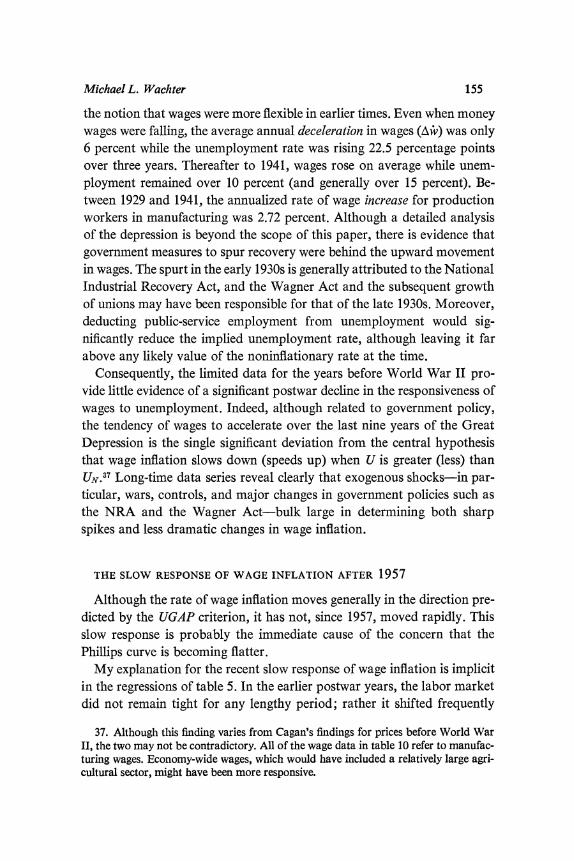
Michael L. Wachter 155
the notion that wages were more flexible in earlier times. Even when money wages were falling, the average annual deceleration in wages (A;V) was only 6 percent while the unemployment rate was rising 22.5 percentage points over three years. Thereafter to 1941, wages rose on average while unem- ployment remained over 10 percent (and generally over 15 percent). Be- tween 1929 and 1941, the annualized rate of wage increase for production workers in manufacturing was 2.72 percent. Although a detailed analysis of the depression is beyond the scope of this paper, there is evidence that government measures to spur recovery were behind the upward movement in wages. The spurt in the early 1930s is generally attributed to the National Industrial Recovery Act, and the Wagner Act and the subsequent growth of unions may have been responsible for that of the late 1930s. Moreover, deducting public-service employment from unemployment would sig- nificantly reduce the implied unemployment rate, although leaving it far above any likely value of the noninflationary rate at the time.
Consequently, the limited data for the years before World War II pro- vide little evidence of a significant postwar decline in the responsiveness of wages to unemployment. Indeed, although related to government policy, the tendency of wages to accelerate over the last nine years of the Great Depression is the single significant deviation from the central hypothesis that wage inflation slows down (speeds up) when U is greater (less) than UN.37 Long-time data series reveal clearly that exogenous shocks-in par- ticular, wars, controls, and major changes in government policies such as the NRA and the Wagner Act-bulk large in determining both sharp spikes and less dramatic changes in wage inflation.
THE SLOW RESPONSE OF WAGE INFLATION AFTER 1957
Although the rate of wage inflation moves generally in the direction pre- dicted by the UGAP criterion, it has not, since 1957, moved rapidly. This slow response is probably the immediate cause of the concern that the Phillips curve is becoming flatter.
My explanation for the recent slow response of wage inflation is implicit in the regressions of table 5. In the earlier postwar years, the labor market did not remain tight for any lengthy period; rather it shifted frequently
37. Although this finding varies from Cagan's findings for prices before World War II, the two may not be contradictory. All of the wage data in table 10 refer to manufac- turing wages. Economy-wide wages, which would have included a relatively large agri- cultural sector, might have been more responsive.

156 Brookings Papers on Economic Activity, 1:1976
from tightness to slack. In this type of environment, inertia or expectation effects had little time to build, and short-run movements in wage inflation were dominated by movements along a given narrow band of Phillips curves. The result, reinforced by the long lags onpi or mhl, was a relatively flat series of wage increases. With the long period of slack after 1957 and the long tight period after 1965, the long lags on the price (or money-supply) term built momentum and hence played a bigger role in determining the rate of wage inflation. As the equations indicate, the momentum, or heri- tage, in the p1 or mhl terms acts to override cyclical swings in UGAP and hence to weaken the "observed" cyclical pattern of wage inflation. This effect is quite separate from the impact of unemployment on inflation. Figure 3, which depicts the UGAP and fil components of wage inflation since 1954, based on equation 5.2, illustrates these arguments. A similar picture and conclusions would follow if the decomposition reflected an equation containing mhl in place of pl.
The figure shows that in the cyclical downturns of 1954, 1957, and 1960, the heritage effects of pl and UGAP moved in essentially the same direc- tion. At the time of the preceding peak, no large heritage effects of accel- erating prices had built up, and thus the price variable turned down promptly, reinforcing the short-run impact of unemployment. The 1956-57 experience also benefited from the dissipation of the effects of the Korean War price explosion, in terms of the estimated lag structures, so that the price variable exerted a major downward influence. The effect is to make wage inflation appear sensitive to cyclical swings in unemployment. In the early 1960s, aggregate-demand policies were able to drive unemployment down without any significant increase in inflation because the pl effect continued to fall, and U remained above UN. The final three years of the 1960s saw accelerating wage inflation as falling unemployment rates were gradually augmented by a rising p1 effect.
The 1970 recession broke from the pattern of earlier recessions because of a buildup of lagged excess-demand effects in the price term. Although the UGAP contribution to wage inflation fell precipitously, the pI effect continued to rise. Whereas in earlier downturns p1 aided UGAP, beginning in 1970 it fought the UGAP effects. The 1972 plateau in p1 implies, how- ever, that if the recession had continued a little longer, or if U had not fallen below UN, the price effect finally would have helped to slow the in- flation rate. This same pattern has prevailed in 1974-75. Although UGAP is, in a sense, working harder than ever to slow the inflation, the legacy of

4-
C~~~~~~~~~ l
(ON
C-~~~~~~~~~~~~~~~~~~~~~~~~~~~~~~~~~~~~~~~~~~~~~~~~~~~~~~~~~~~~~~~~~~~~~~~~~~1 ON
0 . t
'5z1
C-.......1
CO 0 *

158 Brookings Papers on Economic Activity, 1:1976
nearly a decade in which U was typically less than UN, built into the lags in pl (or mhl), has prevented any significant downturn in wage inflation. According to this interpretation, current unemployment does work to slow inflation, but its efficacy depends upon the heritage of past excess demand that is built into the lag structures.
Conclusion
The major conclusion of this paper is that the magnitude of the impact of unemployment and aggregate demand on wage inflation has increased over the postwar period. This result is obtained largely from analyzing structural and reduced-form wage equations. It contradicts the popular view, espoused in the academic literature and financial press, that wages are becoming less sensitive to aggregate-demand policies.
The impression that wage inflation is less responsive to unemployment arises from two factors. First, as indicated in tables 1 and 4, wages are in fact less responsive to measured unemployment; but they do not show lessened sensitivity when a weighted unemployment series-for example, UGAP-is used as the demand variable. Official unemployment is not an accurate measure of labor-market tightness. Second, as shown in figure 3, in earlier recessions the UGAP and p1 effects reinforced one another, thus confirming the observed cyclical nature of wage inflation. In other words, downward movements along a Phillips curve (as unemployment increased) were strengthened by downward shifts of the short-run Phillips curve. In the past two recessions, on the other hand, UGAP effects have been at least partially offset by large inertia effects which have kept the contribution of the price term rising at least through the early stages of the downturn. Essentially, upward shifts of the Phillips relationship, due to lagged or catch-up effects, dampened the observed wage responsiveness to cyclical swings.
The growing importance of inertia effects is due to the long period of generally tight labor markets after the mid-1960s. The simultaneous rise in the inflation and the unemployment rates noted in 1969-70 is to be ex- pected under such circumstances-the turn in wage-inflation rates lagging far behind the NBER turning point. Hence, the current downturn, al- though slow in yielding its benefits, is likely to provide a period of falling rates of unemployment and inflation. Although the lagged effects of prices
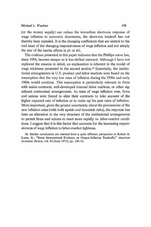
Michael L. Wachter 159
(or the money supply) can reduce the immediate short-run response of wage inflation to economic downturns, the short-run tradeoff has not thereby been repealed. It is the changing coefficients that are central to the real issue of the changing responsiveness of wage inflation and not simply the size of the inertia effects in p1 or ml.
The evidence presented in this paper indicates that the Phillips curve has, since 1954, become steeper as it has shifted outward. Although I have not explored the reasons in detail, an explanation is inherent in the model of wage stickiness presented in the second section.38 Essentially, the institu- tional arrangements in U.S. product and labor markets were based on the assumption that the very low rates of inflation during the 1950s and early 1960s would continue. This assumption is particularly relevant to firms with union contracts, well-developed internal labor markets, or other sig- nificant contractual arrangements. As rates of wage inflation rose, firms and unions were forced to alter their contracts to take account of the higher expected rate of inflation or to make up for past rates of inflation. More important, given the greater uncertainty about the permanence of the new inflation rates (with both upside and downside risks), the response has been an alteration in the very structure of the institutional arrangements to permit firms and unions to react more rapidly to labor-market condi- tions. I suggest that it is this factor that accounts for the increasing respon- siveness of wage inflation to labor-market tightness.
38. Similar conclusions are reached from a quite different perspective in Robert E. Lucas, Jr., "Some International Evidence on Output-Inflation Tradeoffs," American Economic Review, vol. 63 (June 1973), pp. 326-34.

Comments and Discussion
Robert E. Hall: This paper amply repays the concentrated effort required to figure out what is going on inside it. It starts from the conflict between modern theories of wage adjustment, in which rising uncertainty about future inflation should make the wage more responsive to unemployment, and the popular impression that wages are now virtually immune to the influence of unemployment. Wachter demonstrates that casual econo- metrics seems to support the popular view, and then builds a case, relying on a more refined study of the data, that the modern theory is in fact cor- rect. Though I confess that I was predisposed toward Wachter's view, only a detailed examination of his evidence, including some material not covered in the paper, convinced me that the empirical case is, in fact, fairly strong.
Wachter's first criticism of the casual evidence is exactly right, in my view. He observes that the diminishing response of wages to unemployment has been more than offset by a growing response to inflationary expecta- tions as captured in lagged prices. The true impact of unemployment on wages should be measured to include both the direct effects and the in- direct effect operating through prices.
The next step in the case is the introduction of a normalized measure of unemployment in place of the official unemployment rate. Like George Perry's pioneering work, this adjustment attempts to eliminate the shifts in unemployment that are attributable to changes in the composition of the labor force rather than changes in inflationary pressures in the labor mar- ket. In fact, Wachter's adjustment goes much further than Perry's. My own approach to the same problem (BPEA, 2:1974) is intermediate between the two. The differences can be iliustrated by considering the effect on the various adjusted unemployment rates of an increase in the number of teen- agers in the labor force that is accompanied by no change in the unemploy-
160

Michael L. Wachter 161
ment rate of any demographic group: the official unemployment rate will rise. Perry's rate wili rise, but not as much, because he weights teenagers by their earnings instead of giving equal weights to all members of the labor force. My unemployment rate will remain exactly unchanged, because it is a fixed-weight index of the age-sex groups. The logic of my measure is that conditions in the labor market as a whole have not changed if there is no change in the unemployment rates of any group. Wachter's nor- malized unemployment rate will actually fall. He expects a change in the composition of the labor force to drive the teenage unemployment rate up; if this fails to happen, he diagnoses a tightening of the labor market. Em- pirical evidence on the choice of adjusted unemployment rates is extremely weak. In Wachter's table 5, Perry's unemployment rate, Up, actually comes out ahead, though unreported results obtained by Wachter favor his own measure. But the data won't give a definitive answer.
Wachter's choice of an unemployment variable has an important role in his case against the flattening Phillips curve. His UGAP variable is defined so that the impact of a one-point increase in the unemployment rate has a smaller effect on wage inflation when UN and U are both high for compo- sitional reasons than when they are both low, even though UGAP itself has the same value. The flattening of the Philips curve on this account is espe- cially important in Wachter's work precisely because his demographic shift is so large.
The centerpiece of Wachter's case is his set of estimates of a Philips curve with all variables measured to his satisfaction, but including a term that lets the curve shift over time. If the popular view is correct, he argues, then the shift should flatten the curve. Instead, the curve steepens. As Robert Solow pointed out, however, most of Wachter's evidence on this point is dubious because the main impact of the shift is to move the Phillips curve upward rather than to change its slope. This problem would arise no matter how the time variable were defined, but Wachter's LT variable makes it particularly serious because it varies so little over the sample pe- riod (from 4.92 to 5.40). As Wachter observes in the section entitled "View- ing the Shift," the appropriate solution to this problem is to let LT shift the intercept as well as the slope of the Philips curve. Then the t-statistic associated with the slope-time trend interaction, LT. UGAP, provides a test of the hypothesis that the Phillips curve has steepened against the alter- native that it has become flatter. Wachter does not report the regression in the paper, but he has told me that the t-statistic is 0.76. There is about one
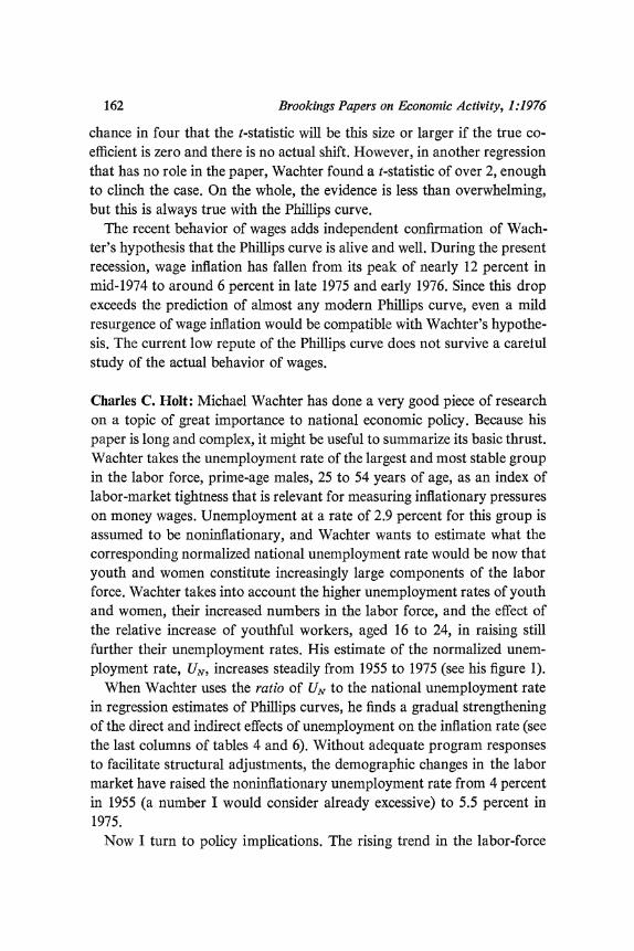
162 Brookings Papers on Economic Activity, 1:1976
chance in four that the t-statistic will be this size or larger if the true co- efficient is zero and there is no actual shift. However, in another regression that has no role in the paper, Wachter found a t-statistic of over 2, enough to clinch the case. On the whole, the evidence is less than overwhelming, but this is always true with the Phillips curve.
The recent behavior of wages adds independent confirmation of Wach- ter's hypothesis that the Phillips curve is alive and well. During the present recession, wage inflation has fallen from its peak of nearly 12 percent in mid-1974 to around 6 percent in late 1975 and early 1976. Since this drop exceeds the prediction of almost any modern Phillips curve, even a mild resurgence of wage inflation would be compatible with Wachter's hypothe- sis. The current low repute of the Phillips curve does not survive a careful study of the actual behavior of wages.
Charles C. Holt: Michael Wachter has done a very good piece of research on a topic of great importance to national economic policy. Because his paper is long and complex, it might be useful to summarize its basic thrust. Wachter takes the unemployment rate of the largest and most stable group in the labor force, prime-age males, 25 to 54 years of age, as an index of labor-market tightness that is relevant for measuring inflationary pressures on money wages. Unemployment at a rate of 2.9 percent for this group is assumed to be noninflationary, and Wachter wants to estimate what the corresponding normalized national unemployment rate would be now that youth and women constitute increasingly large components of the labor force. Wachter takes into account the higher unemployment rates of youth and women, their increased numbers in the labor force, and the effect of the relative increase of youthful workers, aged 16 to 24, in raising still further their unemployment rates. His estimate of the normalized unem- ployment rate, UN, increases steadily from 1955 to 1975 (see his figure 1).
When Wachter uses the ratio of UN to the national unemployment rate in regression estimates of Phillips curves, he finds a gradual strengthening of the direct and indirect effects of unemployment on the inflation rate (see the last columns of tables 4 and 6). Without adequate program responses to facilitate structural adjustments, the demographic changes in the labor market have raised the noninflationary unemployment rate from 4 percent in 1955 (a number I would consider already excessive) to 5.5 percent in 1975.
Now I turn to policy implications. The rising trend in the labor-force

Michael L. Wachter 163
participation of women will offset for some time the declining entry of young workers. Given such a trend, this research implies that employment- guarantee programs, public-service employment, or other programs for re- ducing unemployment that are primarily demand-oriented cannot succeed in four years in making noninflationary an unemployment rate of 3 percent, even for adults, without substantial changes in the scope and effectiveness of structural programs and policies in labor and product markets. Thus, in my view, Wachter's research has important implications for improving the regulation of aggregate demand and demonstrating the need for new structural policies in showing the high costs of excessive fluctuations of unemployment in either direction. In addition to showing the need for new manpower, antitrust, and other structural policies, this work shows the relatively low incremental anti-inflation impact of high unemployment and the inflationary risks of low unemployment unless structural reforms are instituted.
Now for some technical points: First, the assumption is made that if UPM were constant, inflationary
pressure would be constant even in the face of changing demographic com- position. However, greater unemployment of women and youths will have some anti-inflationary effect, so UPM would have to be lower to hold infla- tionary pressure constant. Wachter's UN gradually drifts too high, so the coefficient on (UN! U) will gradually drift too low. Hence Wachter may be underestimating the upward trend in that coefficient.
Second, there is a great deal of confusion among both the public and the profession about the Phillips curve, and I am afraid that Wachter's expo- sition will contribute even more. He is clear on the theory, I think, but his discussion still leaves something to be desired. I do not agree with his view that the distinction between direct wage effects and indirect price effects is merely a matter of definition. Multicollinearity makes the theoretical speci- fications critical.
Three sets of relations governing wages, prices, and unemployment are involved in the inflation-unemployment tradeoff. Wachter estimates two relations and makes assumptions about the third. For the policy question that he discusses, a dynamic tradeoff relation combining all three relations is needed.
It is relevant to talk about a long-term tradeoff or a short-term tradeoff, and they will be quite different; but these two concepts should not be con- fused with the lags in wage and price responses. Nowhere is the problem
164 Brookings Papers on Economic Activity, 1:1976
more treacherous than when demand variables are introduced. The growth of the money supply is entered in a wage equation while it belongs in the price equation. Because the price equation isn't treated explicitly, there is no convenient way to bring in commodity-price effects.
I am pleading for more stress on thinking in systems and structural terms rather than trying to cram many issues into a simple Phillips relation. Where an overall reduced-form relation between inflation and unemploy- ment is presented, then dynamics, and exogenous influences such as oil and worldwide failure of grain crops, should be included. Otherwise, the pre- sentation of a simplistic and utterly inadequate Phillips relation is confusing and subject to glib attack based on a two-dimensional scatter plot that purports to demonstrate that there is no relation between inflation and un- employment. Sufficiently misinterpreted, such an approach can be used to discredit the profession. Wachter's mathematical theory is fine, but some of the final figures are very likely to be misunderstood.
General Discussion
The Wachter paper proved to be particularly provocative in eliciting comment from the panel. The author was commended for testing the widely accepted proposition that the Phillips curve had grown flatter in recent years; nobody contested his conclusion that this piece of conventional wis- dom did not stand up well. While these negative findings were seen as im- portant, the positive results that Wachter reported on the steepening of the Phillips curve were viewed skeptically by many participants.
Robert Solow pointed out a particular feature of those equations re- ported in table 5 in which the unemployment variable interacts with time. The specification of those equations forces the curve to become steeper if it shifts up through time; it can only become flatter if it shifts down through time. Such a regression formulation gives the curve no opportunity to pivot around some point in the middle of the range. That option arises only when the intercept, as well as the slope, is permitted to change through time, as in the equations 10 and 11 reported by Wachter. But the statistical results of those equations do not provide solid evidence of steepening.
Robert J. Gordon doubted that the model could accurately distinguish between (1) the shift of the normalized unemployment rate, and (2) the increase in the inflation rate that affects wages with lags through the price

Michael L. Wachter 165
term, since the two have occurred more or less simultaneously. John Sho- ven was disturbed by the sizable quantitative difference between the results obtained with Wachter's UGAP measure and with Perry-weighted unem- ployment, as reflected in figure 2. Edward Gramlich expressed his reserva- tions about the formulation in that figure, which ignored the feedback effect of prices. He preferred findings that did allow for price feedback, such as those summarized in table 7. R. J. Gordon shared this concern, guessing that one would get statistically indistinguishable results with lags of varying length applied to prices and to unemployment. Michael Wachter responded that, in some fundamental sense, the true reduced-form equation should contain infinite lags on the unemployment variable which keep influencing the history of prices; to him, the decision on where the lag on the labor-market variable ended and the price term began is an arbitrary one. Arthur Okun suggested that the bouquet of equations presented in table 5 might be viewed by readers as a demonstration that the interaction term has a positive coefficient regardless of the choice of lags, the unem- ployment variable, or other aspects of the specification.
George Perry emphasized that, according to Wachter's equations, the world had become much more inflationary at any unemployment rate and even at any normalized unemployment rate. If price stability is consistent with wage increases of roughly 3 percent, Wachter's equation 5.4, for example, implied that noninflationary wage behavior would have been obtained with an unemployment rate of less than 31/2 percent in the mid- fifties and would currently require an unemployment rate as high as 7 per- cent. In contrast, equations 10 and 11 suggest that the noninflationary unemployment rate in 1975 was about 51/2 percent, agreeing with Wachter's estimate of UN. But they imply implausibly that an unemployment rate of only 21/2 percent was noninflationary in 1954.
Only a small portion of those shifts could be accounted for by the demo- graphic Shift that affected the normalized unemployment rate; the rest had to reflect some different force which is not explained in the paper. Thus, to Perry, the issue of steepening or flattening was secondary. The big ques- tion was, "What else has been affecting the economy to make it so much more prone to inflation?" Expanding on Perry's comment, James Tobin pointed out that the normalization of the prime-age unemployment rate to 2.9 percent did not really constrain the labor market to the same degree of inflationary behavior at that rate through time. Tobin suggested that an equation could be specified that maintained the hypothesis that such a rate

166 Brookings Papers on Economic Activity, 1:1976
for prime-age males was consistent throughout the period with nonacceler- ating inflation; and that specification could be tested to see whether or not the curve twisted.
R. J. Gordon suggested that a plausible explanation for a large upward shift in the Phillips curve could be built on the assumption that wage changes have become much more responsive to price changes because peo- ple pay more attention to price changes in an inflationary world. Charles Holt found Gordon's conjecture quite plausible; the experience of inflation might have made people quicker on the draw, so to speak, in terms of ad- justing wages to price changes. However, any greater responsiveness in the upward direction would steepen Wachter's equations symmetrically, im- plying more responsiveness in the downward direction as well. In reality, there were good reasons to suspect that an asymmetry existed.
The policy implications of the findings drew comment from Marina Whitman and Shoven. Whitman noted that a steeper Phillips curve ap- peared to imply that the inflation problem was more easily corrected by use of restrictive stabilization policy. But when the instability of the Phillips curve as well as its slope was taken into account, she doubted that one could draw any comfort for policy from the steepening of the curve. Shoven suggested that the results in table 7 pointed to an extremely high social cost of wage deceleration. A deceleration of 2.7 percentage points in the rate of wage inflation required maintaining an 8 percent unemployment rate for four years. That represents a cumulative total of 10 percentage points of annual unemployment above the normalized rate and a total cost of nearly $500 billion, or close to one-third a year's GNP.
Wachter responded to a number of the criticisms and comments. He was in general agreement with the comments by Hall and Holt. He agreed with Holt's suggestion that a full-model approach should shed more light on the problem than a single-equation estimation, although he defended the inclusion of the money-supply variable in the reduced-form approach. Wachter also pointed out that his attempts to represent exogenous events, such as changes in oil and food prices, with dummy variables did not change the outcome of the regressions. He argued that some of the disagreement in the general discussion was over the interpretation of the lagged price term, and he tried to persuade the panel that that term should be inter- preted as a distributed-lag generator of past labor-market conditions. In this light, R. J. Gordon's comment that the increasing responsiveness is due to higher inflation concurs with the paper.

Michael L. Wachter 167
Although Wachter agreed that long recessions had large economic costs, and was not recommending them as a policy, he pointed out that any calculations based on the old notions of a 4 percent full-employment un- employment rate would overstate the costs of unemployment. In any case, his estimates of the cost of reducing inflation, though still large, are lower than the consensus figures.
Wachter agreed with Perry and Solow that it is difficult to distinguish between the effect of changes in the intercept and in the slope of his equa- tions. Wachter felt that other factors besides those directly in the equation could be making the economy more inflation-prone. But, in looking for causes, he would tend to focus on other aggregate-demand factors such as capacity utilization, excess demand in agriculture, and the growing syn- chronization of the business cycle throughout the world.