ISSN: 1439-2305

Number 199 – March 2014

THE CCCTB OPTION – AN

EXPERIMENTAL STUDY

Claudia Keser, Gerrit Kimpel and Andreas Oestreicher

1

The CCCTB option – an experimental study

Claudia Kesera, Gerrit Kimpelb and Andreas Oestreicherc

Abstract:

The objective of this paper is to look into the probability that, given the choice, corpo-

rate groups would opt for taxation on a consolidated basis. Consolidation would allow

them to offset losses crossborder but remove the opportunity to exploit international

tax-rate differentials between entities via transfer pricing. We present a laboratory

experiment in which we investigate to what extent a corporation would be inclined to

take up the consolidation option and how this would impact on the corporation’s lo-

cation of investment and its transfer pricing activities involving locations outside the

consolidated group. We use a 2-by-2 treatment design with two levels of tax-rate dif-

ferential between two investment locations, and two different remuneration functions

allowing the participants to act as owners or managers of a company.

Keywords: International Company Taxation; Separate Accounting; Formula Appor-

tionment; Transfer Pricing; Experimental Economics.

JEL codes: C91, H25, M41.

a University of Göttingen, Department of Economics, Chair of microeconomics, Platz der

Göttinger Sieben 3, 37073 Göttingen, Germany, claudia.keser@uni-goettingen.de

b University of Göttingen, Department of Business Administration, Tax Division, Platz der

Göttinger Sieben 3, 37073 Göttingen, Germany, gerrit.kimpel@wiwi.uni-goettingen.de

c University of Göttingen, Department of Business Administration, Tax Division, Platz der

Göttinger Sieben 3, 37073 Göttingen, Germany, andreas.oestreicher@uni-goettingen.de

2

1 Introduction

In March 2011 the European Commission submitted a draft directive proposing the

introduction of a Common Consolidated Corporate Tax Base (European Commis-

sion, 2011). Under a CCCTB the companies belonging to a corporate group would be

allowed to file one single tax return and consolidate all the profits and losses they in-

cur across the EU. The aim of this proposal is to remove existing tax obstacles to the

development of the internal market. A main issue of the present system, in which

corporations in the EU are taxed separately (separate accounting), concerns the high

costs relating to compliance with transfer-price regulations according to the arm’s-

length principle. In addition, over-taxation arises in cross-border activities where a

cross-border loss offset is only available under certain pre-conditions. What is more,

the network of double taxation treaties grants businesses insufficient protection

against double taxation since such treaties are designed to address bilateral relations.

Under a CCCTB the consolidated tax base would be shared out amongst the member

states in which the corporation is active, according to a specific formula using a com-

bination of tangible fixed assets, labor costs, employment, and sales by destination as

the allocation key (formula apportionment). The CCCTB constitutes a form of group

taxation allowing for a cross-border loss offset, which under the current system of

separate accounting only applies locally in a small number of countries under very

specific conditions. The CCCTB option thus offers some kind of institutional choice,

under which the corporations concerned opt either for tax planning under separate

accounting with no cross-border loss offset but the opportunity for profit shifts, or for

cross-border loss offset with tax planning under formula apportionment. Under for-

mula apportionment, corporations would lose opportunities for profit shifting, and

we might expect consequences for investment (allocation of production factors) and

the choice of location.

Our study investigates the acceptance and effects that introduction of an optional

CCCTB would have on the allocation of investment and usage of specific tax-planning

alternatives available under separate accounting and formula apportionment. In this

case an optional CCCTB means that companies would not be forced to enter the new

system, and hence to carry the costs of switching to this new regime.

Up to now, these questions have been examined only in part. Empirical investigations

have been limited to the domestic context. The impact of ’institutional choices‘ has

been subjected to scant examination as a whole. As a rule, these choices are made on

3

the basis of a complex network of facts and circumstances, for which scarcely any da-

ta emerges that can be scrutinized. Research relating to profit shifting often neglects

the possibility of potential losses in the analysis.1 Since we lack real-life data that

would allow us to analyze the effect of an optional taxation on a consolidated basis,

we use the method of experimental economics. The experimental method has an ad-

ditional advantage. Psychological aspects can be investigated more easily in a con-

trolled laboratory environment than in real-life data. Such aspects play an important

role when it comes to decisions regarding taxes, as has already been pointed out by

Schmölders (1960, 1970). . The controlled laboratory environment is of particular

significance in our experiment due to the complexity of the issue under examination.

Beyond behavioral anomalies that are often observed in cases of decisions made in a

situation of uncertainty, we can investigate, how people deal with complexity extend-

ing beyond their cognitive limits (Simon, 1957).

Our experiment focuses on the choice of tax regime (separate accounting or formula

apportionment), the allocation of production factors, and profit-shifting activities in

the presence of uncertain returns on investment. In a 2-by-2 treatment design, we

consider the impact of two levels of tax-rate differential and of a manager versus an

owner compensation scheme. Several empirical investigations have shown that tax-

rate differentials impact on investment-location and transfer-pricing decisions (see

Section 2 below). The remuneration scheme could play an important role since own-

ers have to bear losses, while managers do not.

With respect to the proposed introduction of a CCCTB, we observe in our experiment

that participants make use of taxation on a consolidated basis in a substantial num-

ber of cases, while at the same time they exploit the benefits of shifting profit to lower

taxed investment alternatives outside the consolidated group. Furthermore, our ex-

perimental results suggest that the use of formula apportionment influences the allo-

cation of economic values taken up in the allocation formula. These findings suggest

that profit shifting will continue to take place and is carried out using the same ave-

nues, i.e., allocation of assets to low taxed investment alternatives and shifting of ‘pa-

per’ profits. However, they also make it clear that formula apportionment provides an

equivalent alternative tax regime since it offers intra-group loss-offset and, hence,

brings with it tax advantages in cases that investments end up in a loss.

1 The influence of taxation on investment under uncertainty is analyzed on a theoretical basis by Mack-

ie-Mason, 1990; Alvarez, Kannianinen and Södersten, 1998; Sureth, 2002; Niemann and Sureth, 2004; Edmiston, 2004; Alvarez and Koskela, 2008; Gries, Prior and Sureth 2012.

4

Our paper is structured as follows. Section 2 provides a brief survey of theoretical and

empirical studies on tax-planning strategies under separate ac-counting and formula

apportionment. In Section 3 we present a static model on the impact of the tax re-

gime (separate accounting and formula apportionment) on the optimal allocation of

production factors and tax planning activities making use of profit shifting to low-tax

jurisdictions. Section 4 describes the experimental design and develops our research

hypotheses. Section 5 brings out the results of our analysis. Section 6 concludes.

2 Literature

Institutional settings involving tax planning either under separate accounting or for-

mula apportionment have been the object of a number of empirical investigations.

Many of these investigate the impact of tax rates on choice of investment location and

intra-group transfer pricing under separate accounting. Losses, the possibilities to

off-set losses, or other non-debt tax shields2 have been granted relatively little atten-

tion, though.

Arachi and Biagi, 2005, Hanlon and Heitzman, 2010 and Feld and Heckemeyer,

2011, report on the impact of tax differentials on investment location decisions.

Moreover, the possibilities of using tax differentials by way of transfer pricing are ex-

amined (1) directly on the basis of given market prices or transaction volumes (Ber-

nard and Weiner, 1990; Swenson, 2001; Clausing, 2003), or (2) indirectly via report-

ed profits or profitability, and are shown both for the USA (Grubert and Mutti, 1991;

Harris, 1993; Klassen et al., 1993; Harris et al., 1993; Collins et al., 1998; Klassen and

Laplante, 2012), and the OECD (Bartelsman and Beetsma, 2003) as well as for Eu-

rope (Huizinga and Laeven, 2008; Egger, Eggert and Winner, 2010 and Dharmapala

and Riedel, 2013).3

Devereux, 1989 and Devereux, Keen and Schiantarelli, 1994 consider the influence of

asymmetric taxation of profits and losses on investment decisions. Dreßler and

Overesch, 2013 deal with the impact of existing loss-carry forwards and the treatment

of future losses on the extent of German outbound investment.

In the context of capital structure, the impact of any losses or loss carry-forwards has

been largely neglected. In some cases this influence is taken into account using a bi-

2 See, for example, the current OECD “Action Plan on Base Erosion and Profit Shifting” (OECD 2013a,

2013b) for more sophisticated approaches. 3 In the scope of a meta study Heckemeyer and Overesch, 2013 calculate a semi elasticity of EBIT in

relation to the statutory tax rate of 1.3.

5

nary regression variable that controls for existence or non-existence of loss carry-

forwards (Ramb and Weichenrieder, 2005; Buettner, Overesch and Wamser, 2011).

In order to avoid generating distorted results, losses or tax loss carry-forwards are

also, for the most part, also neglected or explicitly omitted from the analysis, also

when it comes to looking into profit shifting via transfer pricing (Klassen et al., 1993;

Huizinga and Laeven, 2008 and Dharmapala and Riedel, 2013). To our knowledge,

only Creedy and Gemmel, 2011 have given specific scrutiny to loss-making companies

up to now. These authors show analytically that tax-rate sensitivity of tax revenue

decreases the more asymmetrical the tax system becomes.

Offsetting losses against profits is of central importance when businesses are deciding

whether to opt for a group taxation regime, which allows for domestic intra-group

loss-offset, regarding taxes levied on a federal level (where there is no tax differen-

tial). In this context it is shown that with regard to a federal corporate income tax, on

a domestic level companies opt for group taxation if this is advantageous for them in

the interests of improved loss-offset (Oestreicher und Koch, 2010). Companies with

cross-border activities interpose significantly more often than not pure holding com-

panies in their host countries wherever group taxation is available (Mintz and

Weichenrieder, 2010; Oestreicher and Koch, 2012).

The determination of profits under formula apportionment is based on some form of

group income resulting from consolidation or combination of income arising at the

level of the group companies involved. As a general rule, such consolidation or com-

bination includes offsetting profits against losses earned or suffered by the companies

concerned. Besides, the consolidation or combination of income removes all incen-

tives to undertake profit shifting by way of intra-group finance or transfer pricing.

Instead, in such a regime the corporate income tax takes the form of separate taxes

on the factors included in the allocation formula (Mintz, 1999; McLure, 1980). This

implies that where allocation factors relate to company parameters, companies can

use this to optimize the distribution of these amounts across the individual tax juris-

dictions. This feature influences decisions relating to economic values (allocation

ofassets, payroll costs, number of employees and/or sales volume, for example) un-

derlying the allocation formula in a highly complex manner (Gordon and Wilson,

1986). Gérard (2006, 2007) expects the tax-rate sensitivity of investment to increase

if the definition of the formula is based predominantly on a factor that is under the

control of the multinational.

6

In contrast to separate accounting there are few empirical studies on tax plan-ning

and the impact of differences in tax rates and formula weights on company decisions

under formula apportionment. Existing analyses are based to a large extent on data

from the U.S. and Canada (Weiner, 1994; Klassen and Shackelford, 1998; Grubert

and Mutti, 2000; Goolsbee and Maydew, 2000; Gupta and Hofmann, 2002;

Edmiston, 2002, and Edmiston and Arze del Granado, 2006). Mintz and Smart, 2004

find that taxable income of companies under separate accounting varies with tax

rates to a significantly larger extent than taxable income of entities using formula ap-

portionment, which indicates that determining income under separate accounting is

subject to profit shifting.

The tax regimes analyzed do not allow the optional application of either separate ac-

counting or formula apportionment for corporate groups to be considered, as would

be the case if the CCCTB were to be established. In Canada the option of employing

separate accounting or formula apportionment is linked with the choice between a

subsidiary and a branch, which should also be influenced by factors other than taxa-

tion, whereas in the U.S. states under ’unitary taxation‘ formula apportionment is

mandatory with respect to ’unitary businesses‘ if the criteria constituting such unitary

businesses are met.

In Germany, when a commercial enterprise operates in several different municipali-

ties, the trade income of this enterprise in Germany must be allocated to its parts op-

erating in the municipalities concerned according to a given formula (Riedel, 2010;

Büttner, Riedel and Runkel, 2011). For trade-tax purposes, allocation of profits ac-

cording to a formula is also prescribed for tax groups (Büttner, Riedel and Runkel,

2011). Unlike legally and economically independent entities however, since 2002 the

group can opt to fulfill the preconditions of a tax group by concluding a profit and

loss-transfer agreement (i.e., to consolidate profits and losses and apply formula ap-

portionment) or, alternatively, to assess the group companies individually (separate

accounting). In 2001 a reform of corporate income tax had the effect that the costs

associated with non-consolidation for trade tax purposes were increased because

loss-offset opportunities were reduced for those firms that were not consolidated.

Given the fact that non-consolidation involves an increase of costs, in the scope of a

natural experiment for the year 2001 Büttner, Riedel and Runkel, 2011 were able to

examine whether multi-jurisdictional entities increase profit-shifting activities under

a tax system of consolidation and formula apportionment, if this tax system allows

7

individual affiliates to be run as separate entities for tax purposes (‘strategic consoli-

dation‘). Using company data reported in the trade tax statistics for 1998 and 2001,

the authors point out that the varying trade-tax rate among German municipalities

exercises a significantly negative influence on the number of consolidated group

companies. Hence, Büttner, Riedel and Runkel, 2011 consider the choice between

separate accounting and formula apportionment, where possibilities for intra-group

loss offset are given also under separate accounting.

3 A static model of the determination of taxable income

Due to the complexity of the situations examined, which rules out theoretical analysis

using fully fledged models, our experiment consists of four treatments. All situations

involve stochastic elements related to the risk of a loss. Due to tax-loss carry for-

wards, our experiment is based on a dynamic game rather than a simple repetition of

one that remains static. An additional complication in carrying out theoretical analy-

sis relates to the manager (rather than owner) compensation in two of the four treat-

ments: in contrast to owners, managers are not accountable for losses.

In this section we present a static model, without consideration of tax-loss carry-

forwards. We assume that the decision makers are owners and thus accountable for

any losses. This implies that we may consider the first-order conditions for the max-

imization of expected profits without the need to consider any constraints related to

loss situations or very low gains. For this static model we deduce first-order condi-

tions for the allocation of production factors and transfer strategies under each tax

regime. Solutions for the dynamic game versions will be identified in numerical simu-

lations, in which we make use of the first-order conditions (see Section 4.4 below).

3.1 Basic assumptions

The model is based on a fictitious multinational enterprise operating in three coun-

tries called I, II and Z. Each country hosts a subsidiary of this multinational enter-

prise, production sites (called investment objects IO I and IO II) in the countries I

and II, and passive operations (called additional investment object Z) in country Z.

IO I and IO II produce homogenous goods using production factors, R+,

with . For simplicity, we shall not distinguish between labor and capital input,

assuming that they are linked. In country Z the multinational has located passive op-

erations (additional investment object Z), which do not produce real goods. It can

8

only derive income from financial transactions between itself and IO I or IO II, which

can be of interest for tax purposes.

The investment objects in countries 1 and 2 have different profit functions. We as-

sume that each investment object may realize either a gain or a loss, the levels de-

pending on the number of production factors allocated to the respective investment

object. In other words, we assume for each investment object a profit function for the

case of a positive gain, FiG (v

i) and for a loss, FiV (v

i), each depending on the allocation

of the production factors to that investment object. The gain functions have standard-

ized properties, with and . The characteristics of the loss

functions are the same, but with opposite algebraic signs. We assume that a number

of N production factors is available to the multinational enterprise and that these N

factors are to be allocated among the two investment objects. Since it thus holds that

v2 = N – v1, we can express each gain or loss function as a function of . This facilitates

the derivation of the first-order conditions for profit maximization shown below.

Note that the following analyses are based on the assumption of risk neutrality.

The outcomes are presented based on marginal gains and losses (expected marginal

profits) with respect to the number of production factors invested in the same

country i. We simply denote FiG, Fi

V, and FiG’ = dFi

G/dvi, FiV’ = dFi

V/dvi. It holds that

and .

We assume that in each investment object, a gain occurs with the probability p, and a

loss with the residual probability (1 - p). The multinational enterprise’s expected pre-

tax profit, pre-tax, is determined by the sum of expected pre-tax profits in IO I and

IO II, 1 and 2.

(1)

Maximization of the sum of expected pre-tax profits with respect to the number of

production factors in each of the two investment objects would require an allocation

of the production factors such that the expected marginal profit is the same in IO I

and IO II, i.e., 1’ = 2’.

Introducing now the matter of taxation, we assume that gains realized in IO I, IO II or

shifted to Z are taxed at a country specific rate and , respectively. Without loss

of generality, it is assumed that and . Losses do not affect the multina-

9

tional’s tax burden in the specific period. However, losses can be carried forward,

thereby decreasing the tax burden in future periods. As already mentioned above, in

the following analysis, we ignore this effect because a fully-fledged dynamic maximi-

zation that takes the carrying forward of losses into account would be far too complex

to be manageable. We do, however, take account of the possibility to carry forward

losses in our numerical simulations.

In the following, we assume that, prior to its factor-allocation decision and prior to

the realization of positive or negative profits in the two investment objects, the enter-

prise can choose between two exclusive tax regimes, separate accounting (Section

3.2) and formula apportionment (Section 3.3). In Section 3.4, we allow for transfer

pricing and consider optimal strategies under each tax regime.

3.2 Separate accounting

In the case of separate accounting, the profits of IO I, IO II (and Z) are taxed at the

country specific rate (and ), respectively. Note that since no transfer pricing is

included in the analysis at this stage, the profit of the subsidiary located in country Z

is zero.

The expected after-tax profit of the multinational enterprise under separate account-

ing, SA results as follows.

(2)

Maximizing this expression with respect to the number of production factors in each

of the two investment objects leads to the first order condition:

(3)

Maximization of the sum of expected after-tax profits under separate accounting with

respect to the allocation of production factors in each of the two investment objects

requires an allocation such that the expected marginal after-tax profit is the same in

IO I and IO II. In general, if we have internal solutions and if we ignore the fact that

in the experiment factors can only be allocated in integers, this allocation differs from

the optimal allocation pre-tax in that more factors will be allocated to the investment

object with the lower tax rate, which is IO I according to our assumptions above.

10

3.3 Formula apportionment

In the case of formula apportionment the consolidated profits of IO I and IO II are

taxed at a combined tax rate. (The passive operations in country Z are not subject to

consolidation. Profits derived in Z are still taxed at the rate and do not play a role

here.) The weighting of local tax rates, t1 and t2, in the combined tax rate depends on

the sum of wages paid in each of the two investment objects. Since we do not explicit-

ly model the input of labor and capital in a production function, we use the sum of the

marginal profits of each production factor allocated to an investment object as a

proxy for the sum of wages paid in this investment object (under the general assump-

tion that labor is remunerated such that the wage equals the marginal productivity of

labor):

(4)

Based on L1, L2, and t1, t2 the combined tax rate results as

(5)

The expected after-tax profit of the multinational enterprise under formula appor-

tionment FA is as follows:

(6)

Maximizing this expression with respect to the number of production factors in each

of the two investment objects leads to a set of four first-order conditions, depending

on the gain-loss situation in IO I and IO II:

(1) For F1G |F2

V|, F2G |F1

V|:

(7.1)

11

(2) For F1G > |F2

V|, F2G < |F1

V|:

(7.2)

(3) For F1G < |F2

V|, F2G > |F1

V|:

(7.3)

(4) For F1G < |F2

V| , F2G < |F1

V|:

(7.4)

Since FiG and Fi

V are functions of vi, to satisfy the respective first-order condition the

range of vi that determines whether we are in case (1), (2), (3) or (4) needs to be con-

sistent with the range of vi of the respective case. This will lead to a valid solution

within one of the four cases.

3.4 Including transfer-pricing strategies

Under each of the tax two regimes, separate accounting or formula apportionment,

the multinational enterprise has opportunities to reduce the tax burden by way trans-

fer pricing.

3.4.1 Separate accounting

In the case of separate accounting the multinational enterprise has two ways to re-

duce the corporate tax burden. These possibilities may be combined. The first possi-

bility allows the multinational enterprise to shift pre-tax income from the highly

taxed investment object IO II to the lower taxed investment object IO I. This shift of

income is called . The second possibility allows the multinational enterprise to shift

pre-tax income from IO II to the lower taxed additional investment object located in

country Z. This shift of income is called and is taxed at the rate .

12

However, the use of this accounting leeway is not necessarily free of charge. It may be

subject to an audit by tax authorities in country II. If a profit shift between IO I and

IO II (or Z) is detected by the tax authorities, it incurs a subsequent tax payment. The

amount of the additional tax payment is assumed to be the shifted amount from IO II

to IO I or from IO II to the additional investment object , multiplied by the tax

rate differential between IO II and IO I (or ) and multiplied by a penalty factor

(k>1). The probability of an additional payment being charged likewise depends on

the shifted amount, multiplied by a factor or (l1 < 1, lz < 1), respectively.

The overall expected cost of profit shifts under separate accounting, , is:

(8)

The expected after tax profit under separate accounting and under consideration of

profit shifts is as follows.

(9)

The first-order condition for maximizing the multinational enterprise’s expected

profit with respect to the production factors in each of the investment objects re-

quires the consideration of case distinction. These relate to the size of the transfers

relative to the respective potential loss of the object to which the profit has been shift-

ed. In the case of a relatively small transfer, the optimal factor allocation is the same

as without profit shifts. Otherwise, more factors are to be allocated to IO II. The first-

order conditions with respect to the amount of transfer from IO II to IO I are also

dependent on the relationship between the amount transferred and the magnitude of

potential loss:

(10.1)

(10.2)

13

The first-order condition with respect to the transfer from IO II to the additional in-

vestment object is:

(11)

The optimal amount of profit to be shifted to IO I or to the additional investment ob-

ject Z is determined such that the expected marginal tax reduction equals the ex-

pected marginal cost of a profit shift.

3.4.2 Formula apportionment

In the case of formula apportionment the multinational enterprise also has an oppor-

tunity to use intra-firm transactions to reduce the corporate tax burden. It can shift

parts of the aggregated pre-tax profit to the lower taxed additional investment object

located in country Z. This shift of income is called . It is taxed at the rate .

Again, the use of accounting leeway is not free of charge. The amount of an additional

tax payment - in the event that use of accounting leeway between IO II and the addi-

tional investment object is detected - depends on the shifted amount. The shifted

amount is multiplied by the tax rate differential between the combined tax rate of the

tax group and the additional investment object and the penalty factor The

probability of detection depends on the shifted amount, multiplied by the factor

. The expected cost of a profit shift under formula apportionment is:

(12)

Under consideration of penalties, the expected after-tax profit of formula apportion-

ment can be set out as follows:

(13)

This leads to the following first-order conditions for maximizing the multinational

enterprise’s profit with respect to the transfer to the additional investment object in

14

the case of formula apportionment. The result depends on the amount of the transfer

relative to the amount of potential losses and the tax rate differential between the

group and the additional investment object Z.

(1) For F1G |F2

V|, F2G |F1

V|:

(14.1)

(2) For F1G > |F2

V|, F2G < |F1

V| and F1G < |F2

V|, F2G > |F1

V|:

(14.2)

(3) For F1G < |F2

V| , F2G < |F1

V|:

(14.3)

Again the optimal amount of a profit shift is determined such that the marginal tax

reduction equals the expected marginal cost.

4 Experimental design

4.1 Basics

Based on the model presented above, we conduct a laboratory experiment to tackle

the research questions, (1) to what extent corporations would be inclined to take up a

consolidation option under various conditions, and (2) how this would impact the

location of investment and transfer-pricing activities. Over the course of 15 periods,

the participant in this experiment will make individual decisions as the responsible

representative of a group of companies. The experiment consists of a 2-by-2 design,

varying the tax rate differential and the remuneration of the decision maker. Each

treatment involves the choice between separate accounting and formula apportion-

ment, and the possibility of using tax planning strategies associated with these tax

regimes. These strategies include the allocation of production factors and the transfer

of profits from IO II to IO I (under separate accounting), and the transfer of profits

(from IO II or the tax group) to the additional investment object Z.

To present the investment decisions in a manner comparable to the actual situation

of a multijurisdictional enterprise, we need to base our laboratory experiment on re-

alistic input data. For this reason our input factors are linked to (German) company

data (the proportion of profits made and losses incurred by the subsidiaries of a mul-

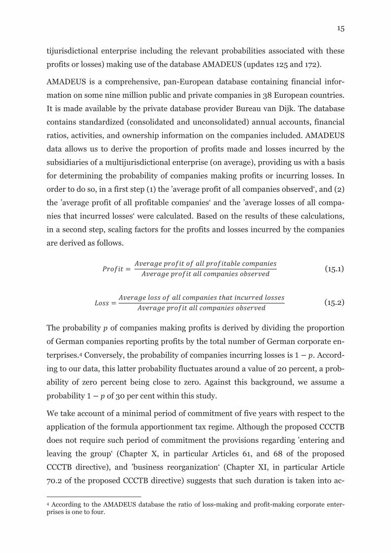
15

tijurisdictional enterprise including the relevant probabilities associated with these

profits or losses) making use of the database AMADEUS (updates 125 and 172).

AMADEUS is a comprehensive, pan-European database containing financial infor-

mation on some nine million public and private companies in 38 European countries.

It is made available by the private database provider Bureau van Dijk. The database

contains standardized (consolidated and unconsolidated) annual accounts, financial

ratios, activities, and ownership information on the companies included. AMADEUS

data allows us to derive the proportion of profits made and losses incurred by the

subsidiaries of a multijurisdictional enterprise (on average), providing us with a basis

for determining the probability of companies making profits or incurring losses. In

order to do so, in a first step (1) the ’average profit of all companies observed‘, and (2)

the ’average profit of all profitable companies‘ and the ’average losses of all compa-

nies that incurred losses‘ were calculated. Based on the results of these calculations,

in a second step, scaling factors for the profits and losses incurred by the companies

are derived as follows.

(15.1)

(15.2)

The probability of companies making profits is derived by dividing the proportion

of German companies reporting profits by the total number of German corporate en-

terprises.4 Conversely, the probability of companies incurring losses is . Accord-

ing to our data, this latter probability fluctuates around a value of 20 percent, a prob-

ability of zero percent being close to zero. Against this background, we assume a

probability of 30 per cent within this study.

We take account of a minimal period of commitment of five years with respect to the

application of the formula apportionment tax regime. Although the proposed CCCTB

does not require such period of commitment the provisions regarding ’entering and

leaving the group‘ (Chapter X, in particular Articles 61, and 68 of the proposed

CCCTB directive), and ’business reorganization‘ (Chapter XI, in particular Article

70.2 of the proposed CCCTB directive) suggests that such duration is taken into ac-

4 According to the AMADEUS database the ratio of loss-making and profit-making corporate enter-prises is one to four.

16

count in order for a multinational enterprise to make full use of potential tax ad-

vantages resulting from a possible allocation of production factors to low-tax coun-

tries. By the same token, German tax law also provides for a minimum commitment

period of five years (Sec. 14 CIT).

The use of tax planning strategies is not necessarily free of charge. They may be sub-

ject to an audit by the tax authorities. If a profit shift is detected by the tax authori-

ties, an additional tax payment results. We assume that the probability of profit shift-

ing being detected is linear in the shifted amount. For profits shifted between IO II

and IO I a probability of 0.00002 is assumed. Profits shifted to the additional in-

vestment object Z is taken into account with a probability of 0.0001.5 As far as penal-

ty payments are concerned reference is made to tax practice in Germany, leading us

to a penalty factor of 1.25 (Section 3.4 above, equations 8 and 12).6 In terms of ex-

pected values, if profit shifting is disregarded, the benefits of an immediate intra-

group loss-offset render formula apportionment the predominant element in multi-

national enterprises’ choice of tax regime. However, since several requirements need

to be fulfilled (e.g., formal requirements associated with the application process, legal

requirements, or additional tax burden resulting from consolidating profits and loss-

es) the formation of a tax group is by no means free of cost. In the experiment we im-

pose a onece only cost for the first-time application of formula apportionment. We

determine the cost level assuming this cost to equal the expected benefit resulting

from the application of formula apportionment over a period of three years. This

means that the expenses associated with the introduction of formula apportionment

are amortized after 60 per cent of the commitment period has elapsed.

4.2 Treatments

We use the tax-rate differential as a treatment variable and consider differentials of

five percent and 15 percent. These tax-rate differentials are designed such that posi-

tive returns in IO I and Z are always subject to a tax burden of 15 percent whereas in

the case of a high tax-rate differential (15 percent) positive returns of IO II are taxed

at a rate of 30 percent and in the case of a low tax-rate differential (five percent) they

are subject to a tax-rate of 20 percent. These differences in corporate tax rates are

5 I.e. the probability of detection increases by 0.1 per cent or 1 per cent, respectively, with each 100 units of profits transferred. 6 According to Sec. 238 German tax code tax payments are charged at a rate of 0.5 percent. Interest is payable starting fifteen months after the end of the relevant tax year. Considering an average tax-audit period of five years (Deloitte 2011), we arrive at a penalty of approximately 25 percent of saved taxes.

17

based on the range of possible tax rates applicable to multinational enterprises within

the European Union.

The participants in the experiment are remunerated based on the profit made by way

of investing in IO I, IO II, and Z. We use remuneration as a treatment variable and

distinguish between two scenarios: the decision maker is either owner or manager.

We take into account the fact that managers are commonly granted bonus payments

only if a pre-determined level of profit is realized. Therefore, in the manager scenario,

their remuneration relates to the return on investment exceeding a predefined (min-

imum) profit after tax (16,000 if the tax-rate of IO II is 30 percent and 18,000 if the

tax-rate of IO II is 20 percent) or is zero otherwise. The conversion factor from profit

to remuneration is determined such that the expected distribution of the remunera-

tion is similar in all treatments.

Note that our theoretical considerations in Section 3 are based on the assumption of a

multinational enterprise seeking to maximize expected profits after tax and bearing

the risk of the actual occurrence of a loss. For companies managed by employees, it

cannot be excluded that different objectives come into play. It is not uncommon for

managers to receive remuneration that is geared to profit. However, it is unusual for

the remuneration scheme to make employed managers liable for losses incurred by

the company (see e.g., Andreas, Rapp, Wolff, 2011). Taking into consideration the

risk of a potential loss may reflect the situation of a transparent entity managed by its

owners. Therefore, in the owner scenario, the design of our experiment is based on

the assumption that the participants in the experiment earn remuneration linked to

the (positive or negative) profit made from investing in IO I, IO II, and Z.

Table 1 presents the parameters of the four treatments.

Table 1: Treatment design

Owner 15 Owner 5 Manager 15 Manager 5

Probability of incurring a

loss (in percent)

30 30 30 30

Remuneration Owner Owner Manager Manager

Tax rate differential 15 5 15 5

18

4.3 Decision-making process

After presenting the instructions (see a translated version of the “instructions manu-

al” in the Appendix A to this paper) to the participants and clarifying any questions,

participants were seated at a computer in the Göttingen Laboratory of Behavioral

Economics and asked to make their individual decisions over the course of fifteen

periods. In each period, the participants had to decide in a first step whether they

wished to opt for separate taxation of the investment objects or group taxation.

Group taxation runs over a sequence of five years. This means that if a participant

had opted for group taxation the choice-of-tax-regime step was unavailable in the

four following periods. After five periods, separate accounting again became an op-

tion.

In the second step, depending on their individual choice of tax regime, the partici-

pants were asked to make an investment decision (allocation of production factors)

and decide whether, and if so, how they wished to make use of accounting leeway.

Allocation of production factors: participants have to allocate N = 15 available pro-

duction factors among IO I and IO II. A minimum of one production factor has to be

invested in each of the two alternative investments objects. The returns of IO I and

IO II differ. For IO II we assume a production function of , where

is the number of production factors invested in IO II. This production function is

characterized by constant marginal returns ( ). For IO I we assume a pro-

duction function of . This production function is char-

acterized by decreasing marginal returns ( ).

Based on the values of and defined in equations 15.1 and 15.2 above, we

may link profits and losses of the investment objects (IO I, and IO II) by a factor of

approximately (e.g. .

Profits and losses depending on the allocation of production factors are presented in

Table 2. A comparable table was included in the written experiment instructions

(which were also read aloud to the participants) and available for view on the com-

puter screen.

19

Table 2: Returns of IO I and IO II

IO I IO II

Number of factors

Profit (p = 70%)

Loss (p = 30%)

Number of factors

Profit (p = 70%)

Loss (p = 30%)

(1) (2) (3) (4) (5) (6)

1 3,091 -2,061 14 42,210 -28,140

2 6,124 -4,084 13 39,195 -26,130

3 9,099 -6,069 12 36,180 -24,120

4 12,016 -8,016 11 33,165 -22,110

5 14,875 -9,925 10 30,150 -20,100

6 17,676 -11,796 9 27,135 -18,090

7 20,419 -13,629 8 24,120 -16,080

8 23,104 -15,424 7 21,105 -14,070

9 25,731 -17,181 6 18,090 -12,060

10 28,300 -18,900 5 15,075 -10,050

11 30,811 -20,581 4 12,060 -8,040

12 33,264 -22,224 3 9,045 -6,030

13 35,659 -23,829 2 6,030 -4,020

14 37,996 -25,396 1 3,015 -2,010

Profit shifts: Where the participants opted for separate taxation of the investment

objects, they had to decide on the profit amount they wished to shift from IO II to

IO I, and on the profit amount they wished to shift from IO II to the additional in-

vestment object. Where the participants opted for formula apportionment, they were

asked to decide on the profit amount they wished to shift from “the group” (IO I and

IO II) to the additional investment object.

The use of tax-planning strategies can be detected by tax-authorities. Both the proba-

bility of being subject to a tax audit and the amount of additional payment depend on

the amount of profits shifted. The amounts of profit shifts related to selected proba-

bilities of being subject to a tax audit (in steps of five percent between five and 100

percent) and the corresponding penalty payments are included in the instructions

manual and are also available for view on the computer screen. Table 3 presents these

numbers for profit shifts to IO I in the case of a tax-rate differential of 15 percent.

Any profit shift was limited by the potential profit in IO II, or, if group taxation was

used, the sum of potential profits in both IOs, given the allocation of production fac-

tors in the first step.

20

Table 3: Probabilities of detection and penalty payments for profit shifts to IO I

Shifted amount Probability of additional payment (percent)

Amount of additional payment

(1) (2) (3)

(1) × 0,00002 (1) × 0.15 × 1,25

0 0 0

2,500 5 469

5,000 10 938

7,500 15 1,406

10,000 20 1,875

12,500 25 2,344

15,000 30 2,813

17,500 35 3,281

20,000 40 3,750

22,500 45 4,219

25,000 50 4,688

27,500 55 5,156

30,000 60 5,625

32,500 65 6,094

35,000 70 6,563

37,500 75 7,031

40,000 80 7,500

42,500 85 7,969

45,000 90 8,438

47,500 95 8,906

50.000 100 9,375

Having entered an investment decision, participants were given the opportunity to

obtain a summary and consequences of their entries by clicking the button “show

consequences”. For the four possible profit-and-loss situations in IO I and IO II

(profit-profit, profit-loss, loss-profit, and loss-loss), depending on their factor alloca-

tion, participants could see the resulting pre-tax results, the amount(s) of profit shift-

ed and the corresponding probability and amount of an additional tax payment. Par-

ticipants were allowed to revise their investment decisions until they pressed the

“ENTER” button. By pressing the button “See results of previous rounds” they had

the opportunity to view their profits and losses accrued in the previous periods.

At the end of each period, participants were informed of their individual profit-loss

situation, any detection of profit shifted, and related additional payment to tax au-

thorities , their net result, and remuneration of the period just completed (in Euro-

cent), and a detailed calculation of net result. Loss carry-forwards in an investment

object are utilized if a profit is accrued in a current period. The amount of losses to be

carried forward was shown on screen at all times.

21

4.4 Deriving theoretical after-tax results

Based on the marginal conditions derived in Section 3 above, the after-tax results in

each of the four treatments were derived by simulating, the decision-making process

10,000 times in the course of the 15-period experiment.7 A simulation approach was

used because due to the dynamic experimental design (caused by the consideration of

losses carried forward) and the large number of maximum conditions to be observed.

The simulation was carried out in such a way that under consideration of losses car-

ried forward and optimal use of tax planning strategies, the investment option was

selected regarding the highest expected return in each of the fifteen periods.8 The re-

sults are presented in Table 4.

Table 4: Simulation results for optimal behavior in the experiment

Owner 15 Owner 5 Manager 15 Manager 5

Pre-tax factor allocation

(IO I/IO II)

2/13 2/13 2/13 2/13

Expected pre-tax return 22,659 22,659 22,659 22,659

Optimal after-tax factor

allocation (SA, IO II)

7.35 8.82 3.78 14

Optimal expected after-tax

return (SA)

18,517 18,596 13,497 11,841

Optimal amounts of profit

shifted (IO II to IO I)

10,670 10,623 2,107 29

Optimal amounts of profit

shifted (IO II to additional

object)

1,430 0 1,290 0

Optimal after-tax factor

allocation (FA, IO II)

6.58 9.22 5.21 14

Optimal expected after-tax

return (FA)

17,295 18,306 13,854 13,380

Optimal amounts of profit

shifted (tax group to addi-

tional object)

621 0 590 0

7 We use Microsoft Visual Basic Application to simulate the optimal behavior. 8 In principle, the optimal profit shift is derived using the first-order conditions presented in the theo-retical model described above. In the case that the model gives rise to negative expected profits, the optimal profit shift is assumed to be zero. If under separate accounting this profit shift exceeds the upper limit of profit earned in IO II less losses carried forward, the value of profits being shifted is reduced to the upper limit. If the loss carry forward of IO II exceeds the profit of IO II, the profit shift is reduced to zero. Under formula apportionment the limitation of profit shifts to the additional in-vestment object is done in the same way as under separate accounting, with the exception that profits and losses being carried forward are aggregated on group level.

22

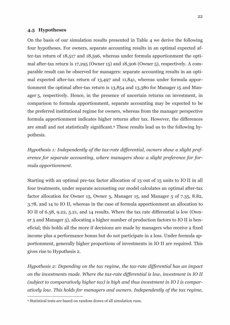
4.5 Hypotheses

On the basis of our simulation results presented in Table 4 we derive the following

four hypotheses. For owners, separate accounting results in an optimal expected af-

ter-tax return of 18,517 and 18,596, whereas under formula apportionment the opti-

mal after-tax return is 17,295 (Owner 15) and 18,306 (Owner 5), respectively. A com-

parable result can be observed for managers: separate accounting results in an opti-

mal expected after-tax return of 13,497 and 11,841, whereas under formula appor-

tionment the optimal after-tax return is 13,854 and 13,380 for Manager 15 and Man-

ager 5, respectively. Hence, in the presence of uncertain returns on investment, in

comparison to formula apportionment, separate accounting may be expected to be

the preferred institutional regime for owners, whereas from the manager perspective

formula apportionment indicates higher returns after tax. However, the differences

are small and not statistically significant.9 These results lead us to the following hy-

pothesis.

Hypothesis 1: Independently of the tax-rate differential, owners show a slight pref-

erence for separate accounting, where managers show a slight preference for for-

mula apportionment.

Starting with an optimal pre-tax factor allocation of 13 out of 15 units to IO II in all

four treatments, under separate accounting our model calculates an optimal after-tax

factor allocation for Owner 15, Owner 5, Manager 15, and Manager 5 of 7.35, 8.82,

3.78, and 14 to IO II, whereas in the case of formula apportionment an allocation to

IO II of 6.58, 9.22, 5.21, and 14 results. Where the tax rate differential is low (Own-

er 5 and Manager 5), allocating a higher number of production factors to IO II is ben-

eficial; this holds all the more if decisions are made by managers who receive a fixed

income plus a performance bonus but do not participate in a loss. Under formula ap-

portionment, generally higher proportions of investments in IO II are required. This

gives rise to Hypothesis 2.

Hypothesis 2: Depending on the tax regime, the tax-rate differential has an impact

on the investments made. Where the tax-rate differential is low, investment in IO II

(subject to comparatively higher tax) is high and thus investment in IO I is compar-

atively low. This holds for managers and owners. Independently of the tax regime,

9 Statistical tests are based on random draws of all simulation runs.

23

in the case of low tax-rate differential, managers will invest the maximum number

of production factors in IOII (Manager 5).

As far as the amounts of profit shifted to IO I (separate accounting) are concerned,

Table 2 indicates the optimal amount shifted is 10,670 for Owner 15 and 10,623 for

Owner 5, whereas the corresponding values are 2,107 and 29 for Manager 15 and

Manager 5. Thus, under the present circumstances, the optimal amount of profits

shifted to IO I differs between owners and managers: managers shift less than own-

ers. Moreover, the shifted amount is expected to be (slightly) higher where the tax

rate differential is high. This leads us to Hypothesis 3:

Hypothesis 3: The amount of profits shifted between group companies is (a) posi-

tively correlated with the tax-rate differential and (b) depends on the remuneration

of the decision makers. Owners will shift higher amounts between group companies

than managers.

Under separate accounting shifting profits to an additional project is countered by a

higher risk of retrospective tax payments then shifting profits to IO I. Hence, profit

shifting to an additional object appears to be beneficial only if the tax rate differential

is sufficiently large: Table 2 shows that for owners the optimal amount is 1,430 and 0

(Owner 15, Owner 5), whereas the corresponding values are 1,290 and 0 for managers

(Manager 15, Manager 5). Since formula apportionment is characterized by a mixed

tax rate, the relevant tax rate differential is larger under separate accounting than

under formula apportionment. As a consequence, the optimal amounts of profit shift-

ed to an additional project fall below the values under separate accounting (621, 0,

590, and 0). These findings lead to Hypothesis 4.

Hypothesis 4: The amount of profits shifted to an additional investment object is

positively correlated with the tax rate differential. Furthermore, owners will shift

higher amounts than managers.

5 Results

Our results are based on computerized experiments conducted at the Göttingen La-

boratory of Behavioural Economics (GLOBE). The experiment was programmed and

conducted with the experiment software z-Tree (Fischbacher, 2007). A total of 83

24

students, 23, 18, 20 and 22 students in treatments Owner 15, Owner 5, Manager 15

and Manager 5, respectively, most of whom attend programs in business

administration and business economics, participated in our experiments. Out of the

83 participants, 24 are female and 59 male. They were randomly selected out of a

pool of students who had signed up for potential participation in experiments (upon

invitation). The student participants earned between 11.00 Euros and 22.10 Euros,

the average being 17.71 Euros.

5.1 Econometric setting

The analyses of the choice of tax regime (Hypothesis 1), the allocation of production

factors (Hypothesis 2), and amount of profit shifed (Hypotheses 3 and 4) are based

on three econometric models.

Regression model 1: Since the choice of tax regime (Hypothesis 1) is binary it is

analysed by way of probit regression including cluster robust standard errors relating

to single individual participants. We use cluster robust standard errors because our

dataset includes several observations for each individual. It can be expected that

standard errors are correlated on an individual basis.10

Regression model 2: The allocation of production factors (Hypothesis 2) is

investigated by way of a zero-truncated negative binomial regression model. Again,

cluster robust standard errors are used. A zero truncated regression model is

appropriate because participants are free to allocate between one and fourteen

countable production factors to IO I or IO II. We used a negative binomial model

instead of the regular poisson model because a test of equidispersion rejects the ‘null’

hypothesis at a one-percent level.11

Regression model 3: The econometric examination of profits shifted to IO I

(Hypothesis 3) or Z (Hypothesis 4), respectively, is based on a linear panel data

model. We employ the natural logarithm of profit shifts in order to reduce the

influence of outliers. Again, cluster robust standard errors are used in respect of each

individual.

Typically, fixed-effect models are applied to exclude unobservable time invariant

individual effects. In our study the use of a fixed effects model is not applicable

10 The Wooldridge test (Wooldridge, 2010) for autocorrelation indicates the existence of autocorrela-tion at a ten-percent level. 11 The existence of overdispersion is tested in an analogous way, following Cameron and Trivedi, 2010.

25

because in this case our time invariant treatment variables (remuneration and tax

rate differential) would be omitted. Because of this we use a random effects model.

Table 5: Description of independent variables

Variable Description Explanatory statement

FA 0 = SA / 1 = FA Selected tax regime might influence the amounts of profits shifted or allocation of production factors

Transfer to IO I Amount shifted to IO I scaled in units of 1,000

Volume of profit shifting activities to IO I might have an effect on the allocation of production factors or profit shiftings to Z

Transfer to Z Amount shifted to Z scaled in units of 1,000

Volume of profit shifting activities to Z might have an effect on the allocation of production factors or profit shiftings to IO I

Investment in IO II Production factors allocated at IO II

Amount invested in IO II might influence profit shifting activities to IO I and / or Z

LCF at IO I, IO II or group level

Amount of losses carried forward at the level of IOI, IO II or scaled in units of 10,000

Existing loss carry-forwards might prevent a switch in tax regime, reduce amount of profit shifting or change the allocation of production factors to reduce loss carry forwards

TD15

0 = Tax-rate differential of 5% / 1 = Tax-rate differential of 15%

Treatment variable

Time Decision making time Longer time of investment represents more detailed tax planning and therefore influences decision making process

Period 1 to 15 Control for time effects for example more conservative decisions in later periods

Manager 0 = Owner / 1 = Manager Treatment variable

Detection of transfer(s) in prior period

0 = no detection in prior period / 1 = detection in prior period

Regarding prior research (Mittone, 2006) detection of tax planning in prior period influences tax planning in the current period

Master 0 = Bachelor 1 = Master Control for different levels of experience

Gender 0 = Female / 1 = Male Control for gender differences

Business experience 0 = No / 1 = Yes Control for different levels of experience

Tax return prepared 0 = No / 1 = Yes Control for different levels of experience

Risk level 0 = Low up to 7 = High Control for self-estimated risk-taking

Impulsivity 0 = Low up to 7 = High Because of a high complex setting, this variable should control for spontaneous decisions

Age Age of participant Control for different levels of experience

Program of study (business administration, economics, other)

Dummy variables equal 1 if participants take part in programs mentioned

Control for different levels of experience in the case of investment decision

Use of such a model produces biased results if time invariant unobservable individual

effects are correlated to other explanatory variables (omitted variable bias). To

prevent such distortions we controlled for a number of individual characteristics.

These were collected via an ex-post questionnaire following the decision-making part

of the experiment. The control variables included, which are intended to absorb

26

distortions resulting from unobserved individual effects or explain individual

behavior, are presented in Table 5. This table also provides a description of

independent variables used in the regressions.

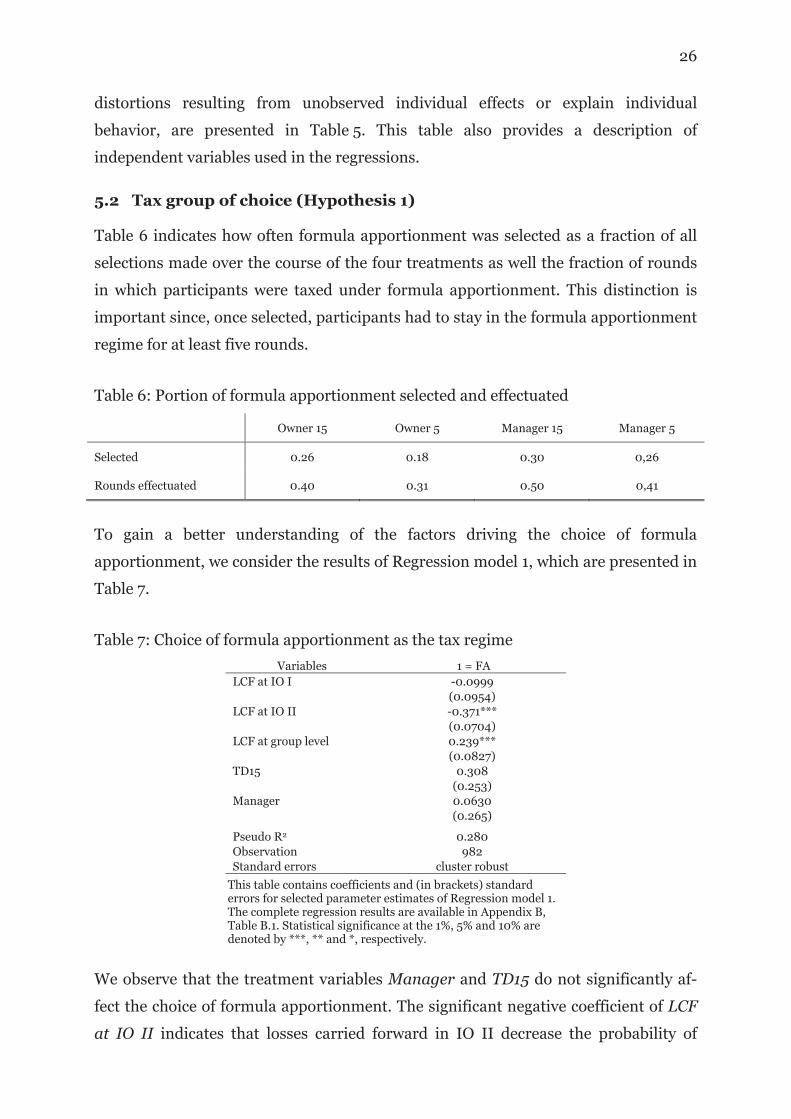
5.2 Tax group of choice (Hypothesis 1)

Table 6 indicates how often formula apportionment was selected as a fraction of all

selections made over the course of the four treatments as well the fraction of rounds

in which participants were taxed under formula apportionment. This distinction is

important since, once selected, participants had to stay in the formula apportionment

regime for at least five rounds.

Table 6: Portion of formula apportionment selected and effectuated

Owner 15 Owner 5 Manager 15 Manager 5

Selected 0.26 0.18 0.30 0,26

Rounds effectuated 0.40 0.31 0.50 0,41

To gain a better understanding of the factors driving the choice of formula

apportionment, we consider the results of Regression model 1, which are presented in

Table 7.

Table 7: Choice of formula apportionment as the tax regime

Variables 1 = FA

LCF at IO I -0.0999

(0.0954)

LCF at IO II -0.371***

(0.0704)

LCF at group level 0.239***

(0.0827)

TD15 0.308

(0.253)

Manager 0.0630

(0.265)

Pseudo R2 0.280

Observation 982

Standard errors cluster robust

This table contains coefficients and (in brackets) standard errors for selected parameter estimates of Regression model 1. The complete regression results are available in Appendix B, Table B.1. Statistical significance at the 1%, 5% and 10% are denoted by ***, ** and *, respectively.

We observe that the treatment variables Manager and TD15 do not significantly af-

fect the choice of formula apportionment. The significant negative coefficient of LCF

at IO II indicates that losses carried forward in IO II decrease the probability of

27

switching the tax regime and choosing formula apportionment. Transforming the

factor value of -0.371 into a marginal effect at the mean of LCF at IOII leads to a val-

ue of 9.5 percent. This implies that the probability of choosing formula apportion-

ment would be reduced by 9.5 percent for each 10,000 units of losses carried for-

ward. A similar influence of losses carried forward can be observed for switches from

formula apportionment to separate accounting: the coefficient of LCF at group level

is significantly positive. The marginal effect of LCF at group level indicates that the

probability of choosing separate accounting would be reduced by 6.1 percent for each

10,000 units of losses carried forward.

To summarize, participants show a slight, though not significant, preference for

separate accounting. Nonetheless, formula apportionment was considered a relevant

option. Neither the tax-rate differential (TD15) nor the compensation scheme (Man-

ager) is shown to drive the choice of tax regime. Losses carried forward (LCF at IO II

and LCF at group level) prevent switching between tax regimes.

What novel insights can be derived from these results? From the perspective of the

authors, the results indicate that formula apportionment provides an equivalent al-

ternative tax regime if risk of investment ending up in a loss is taken into account. In

interpreting this result, we should bring to mind the fact that empirical literature re-

veals transfer pricing to provide an avenue for profit shifting to lower taxing jurisdic-

tions. What is more, looking at profitable companies empirical studies have shown

that the tax-rate differential encourages profit-shifting activities available under sep-

arate accounting. In contrast, under formula apportionment companies optimize the

distribution of factors entering the allocation formula across the individual tax juris-

dictions. This latter planning route is, however, thought to be more expensive and

may also distort investment decisions. Separate accounting is therefore considered to

be more flexible with the result that the literature raises expectations for separate

accounting to be more advantageous where the tax rate differential is larger. On this

note, Mintz and Smart, 2004 find that taxable income of companies under separate

accounting varies with tax rates to a significantly larger extent than taxable income of

entities using formula apportionment. Likewise, Oestreicher and Klett, 2013, show

that the tax rate differential exerts a significantly negative impact on the decision to

opt for group taxation. The lacking influence of TD15 in the regression suggests that

above mentioned advantages of separate accounting are diminished in the presence

of uncertainty. This may be due to the possibility of offsetting losses against profits

28

between investment alternatives under formula apportionment and the correspond-

ing non-debt tax shield representing an equivalent to the potential tax planning ad-

vantages under separate accounting. These findings are supported by the observa-

tions in Büttner, Riedel, und Runkel, 2011, Oestreicher and Koch, 2010, Oestreicher

and Klett, 2013 and Mintz and Weichenrieder, 2010.

The negative influence of losses carried forward on switches between taxregimes

comes as no surprise because a switch would delay offsetting losses against future

profits at least temporarily delay, and thus be accompanied by negative tax effects.

To conclude, in the presence of an optional formula apportionment, the choice of tax

regime depends neither on the remuneration function nor on the tax-rate differential,

but is driven by individual possibilities to offset losses.

5.3 Tax-rate differential and factor allocation (Hypothesis 2)

Table 8 provides the mean values of investments in the higher taxed IO II observed in

each of the four treatments.12 Obviously, in the case of a low tax-rate differential

participants allocate a larger number of production factors to IO II than in the case of

a high tax-rate differential. These differences are statistically significant under both

separate accounting and formula apportionment, and are independent of manager or

owner compensation (for each pairwise comparison, a Wilcoxon-Mann-Whitney

test13 shows significant differences on a five-percent level).

Table 8: Investments in IO II (mean)

Owner 15 Owner 5 Manager 15 Manager 5

Separate accounting 6.72 9.29 6.83 8.65

Formula apportionment 4.35 8.14 7.32 9.75

Table 8 also indicates that for owners investments under formula apportionment fall

below those under separate accounting, while the opposite is true for managers.

However, the difference is statistically significant only in the case of formula

apportionment and the high tax-rate differential (Wilcoxon-Mann-Whitney test, five-

percent significance required).

12 There is no need to consider separately the investment in IO I, since . 13 Due to the requirement of independence between observations, we based the Wilcoxon-Mann-Whitney tests on the individual averages of the number of factors allocated to IO II.

29

Table 9: Allocation of production factors to IO II

Variables Overall SA FA

LCF at IO I -0.0546 -0.0983*

(0.0434) (0.0513)

LCF at IO II 0.0231* 0.0249**

(0.0126) (0.0119)

LCF at group level 0.00957 0.0105

(0.0215) (0.0252)

TD15 -0.343*** -0.240** -0.546***

(0.0933) (0.108) (0.147)

Manager -0.126 -0.106 0.498***

(0.0860) (0.0777) (0.174)

FA -0.237*

(0.122)

FA * Manager 0.595***

(0.169)

Transfer to IO I 0.0256*** 0.0227***

(0.00532) (0.00446)

Transfer to Z 0.0245*** 0.0325*** 0.0257***

(0.00568) (0.00786) (0.00877)

Detection of transfer to IO I 0.00273 -0.0178

(0.0622) (0.0548)

Detection of transfer to Z -0.0156 0.0392 -0.101

(0.0742) (0.0663) (0.138)

Observation 1.245 738 507

Standard errors cluster robust cluster robust cluster robust

This table provides coefficients and standard errors for selected parameter estimates of Regression model 2. The complete regression results are available in Appendix B, Table B.2. Statistical significance at the 1%, 5% and 10% are denoted by ***,** and *, respectively.

The results of Regression model 2 concerning the number of production factors allo-

cated to IO II are presented in Table 9. They indicate a significantly negative coeffi-

cient of TD15, implying that a higher tax-rate differential leads to a significantly lower

investment in the higher taxed IO II, under both separate accounting and formula

apportionment. Since the coefficients of a count data model can be interpreted as

semi-elasticity it emerges that an increase in tax rates by 10 percent leads to 3.43 per-

cent and 5.46 percent less investment under separate accounting and formula appor-

tionment, respectively. It can be seen that under formula apportionment participants

remunerated as managers invest significantly more production factors in IO II than

owners. Their investment is nearly 5 percent higher compared to that made by own-

ers. In the case of owner-based compensation, the use of formula apportionment

leads to significantly lower investment in IO II than under separate accounting (mi-

nus 2.37 percent). The results also make it clear that profit shifting to IO I (Profit

shift to IO I) and Z (Profit shift to Z) is accompanied by larger investments in IO II

(significantly positive coefficients). Under separate accounting a profit shift of 1,000

units to IO I or an identical shift to Z are associated with 2.56 percent or 3.25 percent

30

higher investment in IO II. Under formula apportionment a profit shift to Z increases

investment by 2.57 percent.

To summarize, the allocation of production factors is a function of the tax-rate differ-

ential, under both separate accounting and formula apportionment. Furthermore, the

allocation of production factors is driven by the remuneration function. Under for-

mula apportionment, managers invest higher amounts in the higher taxed investment

object IO II than owners. Besides, the results show that a more extensive use of tax-

planning alternatives leads to larger investments in high tax countries.

What is the conclusion that can be drawn from these observations? One is that in-

vestment is sensitive to the tax rate or a tax rate differential also under the separate

accounting tax regime. A second conclusion is that this sensitivity depends on wheth-

er the entity is driven by owners (the SME or family business) or managers (the busi-

ness of large enterprises). Although the first result is well documented by empirical

studies looking at the impact of taxation on foreign direct investment (see, in particu-

lar, Feld and Heckemeyer, 2013), when focusing on profit or the profitability of com-

panies in low taxed jurisdictions, the corresponding literature on profit shifting, how-

ever, is unable to distinguish between the shifting of ‘paper profits’ and the interna-

tional allocation of highly profitable, in particular intangible, assets. Our study re-

veals that under separate accounting, profit shifting is facilitated to a large extent by

attribution of assets. Although this should be clear when taking on board the fact that

arm’s length pricing is based on comparability factors, including in particular the al-

location of functions, assets, and risks, empirical literature does not make this clear.

Hence, the option between separate accounting and formula apportionment does

bring with it the alternative of shifting profit or shifting assets. The difference is in the

intensity to which assets are shifted to low tax countries.

In this context, we observe that the effect of the tax-rate differential is greater under

formula apportionment than under separate accounting. From a policy perspective,

this greater influence is important because a change in the allocation of production

factors means changing the allocation formula (in our experiment the numbers of

employees as required by the technology underlying the production function). Re-

garding an optional formula apportionment regime this would suggest that the eco-

nomic values underlying the allocation formula will be allocated to low tax countries.

With respect to the difference between decisions made from the manager or owner

perspective, the more intensive investment in the higher taxed IO II by managers as

31

compared with owners might be traced back to the different tax rates applicable in

the separate accounting and formula apportionment contexts. Profits in IO II are

taxed at a lower combined tax rate under formula apportionment than under separate

accounting. In the case that IO II incurs losses the amount of these losses increases

with the number of production factors invested. In contrast to owners, managers do

not have to bear any loss. This leads to larger investments by managers than by own-

ers in the more productive investment object IO II. Owners tend to allocate produc-

tion factors in a more risk-avoiding manner, splitting available production factors

more equally between IO I and IO II because making losses would directly reduce

their compensation.

The positive relationship observed between profit shifting and investments in IO II

suggests that corporations deal with the tradeoff between productivity and taxation

by making use of tax-planning activities. This can have interesting political implica-

tions: by “closing one’s eyes” to profit shifting, additional investment can be attract-

ed.

5.4 Transfer to IO I (Hypothesis 3)

This kind of intra-group transfer applies only to separate accounting. As to the factors

influencing the amounts of profit shifted intra-group, a first issue concerns the tax

rate differential. We expect that the amount of profits shifted between group compa-

nies is positively correlated with the tax rate differential (Hypothesis 3a). A second

issue concerns the existing remuneration scheme. Where decisions are made from

the owner perspective, the amounts of profits shifted to low-tax jurisdictions are ex-

pected to be higher than is the case where the decisions are made by managers who

receive a fixed income plus a performance bonus but do not participate in a loss (Hy-

pothesis 3b).

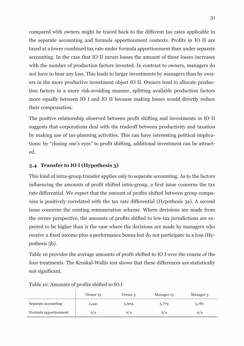
Table 10 provides the average amounts of profit shifted to IO I over the course of the

four treatments. The Kruskal-Wallis test shows that these differences are statistically

not significant.

Table 10: Amounts of profits shifted to IO I

Owner 15 Owner 5 Manager 15 Manager 5

Separate accounting 2,441 5,904 5,779 5,781

Formula apportionment n/a n/a n/a n/a

32

Table 11 presents the results of Regression model 3.

Table 11: Profit shifts to IO 1

Variables LN profit shift to IO 1

LCF at IO I -0.127

(0.0863)

LCF at IO II -0.256***

(0.0750)

TD15 -1.265*

(0.742)

Manager 1.183*

(0.669)

Investment in IO II 0.127**

(0.0498)

Transfer to Z 0.0993

(0.158)

Detection of transfer to IO I 0.713*

(0.392)

Detection of transfer to Z -1.134**

(0.512)

R2 0.265

Observation 738

Standard errors cluster robust

This table contains coefficients and standard errors for selected parameter estimates of Regression model 3. The complete regres-sion results are available in Appendix B, Table B.3. Statistical significance at the 1%, 5% and 10% are denoted by ***,** and *, respectively.

We observe that participants do shift profits to the lower taxed IO I. This profit shift-

ing is higher/lower where the tax rate differentials are low/high (significant negative

coefficient of TD15). We also observe that managers make greater use of accounting

leeway than owners (significant positive coefficient of Manager). The significant pos-

itive coefficient of Investment in IO II indicates that larger investments in IO II is

associated with higher profit shifting activities. Since the coefficients can be inter-

preted in terms of semi-elasticities, it can be inferred that one additional production

factor invested in IO II brings with it increase in profit shifting by 1.27 percent. Large

loss carry-forwards reduce the amount transferred (highly significant coefficient of

LCF at IO II). Specifically, an increase in losses carried forward at IO II by 10,000

units decreases profit shifting by 2.56 percent. Intra-group transfers are also influ-

enced by conducted tax audits in prior periods. A detection of transfers to IO I boosts

profit shifting in future periods by 7 percent (significant positive coefficient of Detec-

tion of transfer to IO I) whereas the fact that income transfer to Z is detected brings

with it to a reduction of profit shifting activities by 11.3 percent (significant negative

coefficient of Detection of transfer to IO Z).

To summarize, the results make it clear that profit shifting to IO I is a function of the

tax-rate differential. Profit shifting to IO I is negatively correlated with the tax-rate

33

differential. What is more, compared to owners, managers tend to transfer higher

amounts intra-group. The detection of profit shifting from IO II to IO I is linked with

higher tax-planning activities in the following periods, whereas the detection of profit

shifts to Z in the prior period leads to the opposite result. Finally, higher investments

in high tax countries give rise to larger transfer pricing activities.

With a view to interpretation: Lower amounts of profits shifted in situations where

the tax-rate differentials are high may reflect the fact that in this case risk of penalty

payments is limited and negative consequences in the case of losses are reduced. To-

gether with the observation that, relative to the simulation outcomes, owners allocate

on average the “right” number of factors to IO II but transfer lower amounts, the ob-

servation that owners shift a lower amount of profit than managers suggests that loss

aversion could play a role (Tversky and Kahnemam, 1979; Kahneman, Knetch and

Thaler, 1990). In addition to a payment reduction in the case of a tax audit, a proba-

bly more painful loss is experienced in the case that profit has been shifted from IO II

to IO I but then a loss occurs (with a probability of 30 percent) in IO II. Since man-

agers are not accountable for losses, they might be more willing than owners to take

the risk of such losses. Note that we do not observe such an effect with regard to

transfers to an additional investment object. Due to the higher detection rate, the

amounts shifted are generally lower there than the transfers to IO I and, specifically,

in the case of formula apportionment the risk of a loss of the group is lower than the

risk of a loss in IO II under separate accounting.

What is more, the possibility of shifting profits from IO II to IO I depends on the

number of production factors previously allocated to IO II (see section 5.3). Besides

the simple relationship that the more profits accrue to the high taxed jurisdiction, the

more profits can be allocated to the lower taxed jurisdiction, this result also indicates

that under separate accounting participants make use of both avenues for profit shift-

ing, i.e., allocating assets to the low taxed investment alternative and shifting ‘paper’

profits. In the latter planning alternative, the participants anticipate the higher

productivity and pre-tax earnings of IO II (instead of making the investment decision

on the basis of post-tax earnings as was shown in section 5.3) and shift this additional

pre-tax profit to the lower taxed investment object IO I. This means that the tradeoff

effect between productivity and tax is reduced by intra-group profit shifting. The neg-

ative correlation between intra-group profit shifting and losses carried forward show

that the reduction of loss carry forwards is preferred to profit shifting activities. This

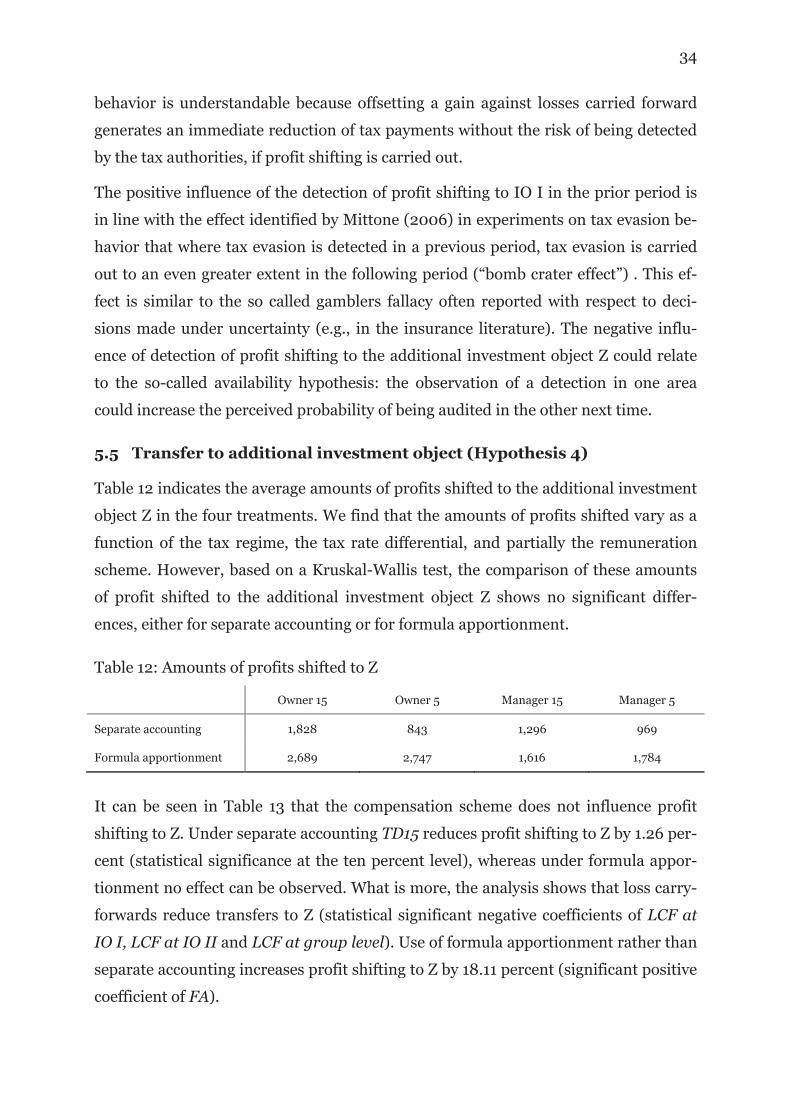
34

behavior is understandable because offsetting a gain against losses carried forward

generates an immediate reduction of tax payments without the risk of being detected

by the tax authorities, if profit shifting is carried out.

The positive influence of the detection of profit shifting to IO I in the prior period is

in line with the effect identified by Mittone (2006) in experiments on tax evasion be-

havior that where tax evasion is detected in a previous period, tax evasion is carried

out to an even greater extent in the following period (“bomb crater effect”) . This ef-

fect is similar to the so called gamblers fallacy often reported with respect to deci-

sions made under uncertainty (e.g., in the insurance literature). The negative influ-

ence of detection of profit shifting to the additional investment object Z could relate

to the so-called availability hypothesis: the observation of a detection in one area

could increase the perceived probability of being audited in the other next time.

5.5 Transfer to additional investment object (Hypothesis 4)

Table 12 indicates the average amounts of profits shifted to the additional investment

object Z in the four treatments. We find that the amounts of profits shifted vary as a

function of the tax regime, the tax rate differential, and partially the remuneration

scheme. However, based on a Kruskal-Wallis test, the comparison of these amounts

of profit shifted to the additional investment object Z shows no significant differ-

ences, either for separate accounting or for formula apportionment.

Table 12: Amounts of profits shifted to Z

Owner 15 Owner 5 Manager 15 Manager 5

Separate accounting 1,828 843 1,296 969

Formula apportionment 2,689 2,747 1,616 1,784

It can be seen in Table 13 that the compensation scheme does not influence profit

shifting to Z. Under separate accounting TD15 reduces profit shifting to Z by 1.26 per-

cent (statistical significance at the ten percent level), whereas under formula appor-

tionment no effect can be observed. What is more, the analysis shows that loss carry-

forwards reduce transfers to Z (statistical significant negative coefficients of LCF at

IO I, LCF at IO II and LCF at group level). Use of formula apportionment rather than

separate accounting increases profit shifting to Z by 18.11 percent (significant positive

coefficient of FA).

35

Table 13: Profit shifts to the additional investment object Z

Variables LN transfer to Z

Overall SA FA

LCF at IO I -0.110** -0.0875

(0.0516) (0.0556)

LCF at IO II -0.146** -0.135*

(0.0739) (0.0702)

LCF at group level -0.262** -0.289**

(0.123) (0.143)

TD15 -0.642 -1.259* -0.118

(0.610) (0.655) (0.801)

Manager 0.299 0.328 0.241

(0.573) (0.636) (0.813)

FA 1.811***

(0.420)

Transfer to IO I 0.0405 0.0600

(0.0396) (0.0451)

Investment in IO II -0.00663 -0.0304 0.0187

(0.0313) (0.0420) (0.0389)

Detection of transfer to IO I 0.0214 -0.151

(0.313) (0.306)

Detection of transfer to Z 0.421 0.112 0.354

(0.298) (0.490) (0.398)

R2 0.195 0.179 0.213

Observation 1.245 738 507

Standard errors cluster robust cluster robust cluster robust

This table provides coefficients and standard errors for selected parameter estimates the main explanatory vari-ables of Regression model 3. The complete regression results are available in Appendix B, Table B.4. Statistical significance at the 1%, 5% and 10% are denoted by ***,** and *, respectively.

To summarize, the difference in tax rates has only a weak (negative) influence on the

transfer to Z if separate accounting is used while according to our simulated solution

presented above, regardless of the remuneration function this relationship should be

positive. Furthermore the results indicate that even where the tax rate differential is

low, participants shift relevant amounts to Z. High impact can be observed with re-

spect to the tax regime (‘FA’). Under formula apportionment the amount of profits

shifted increases substantially. In cases where there are loss carry-forwards, profit

shifting to Z is reduced.

Given the non-existent or at least minor influence of the remuneration function and

the tax-rate differential, we interpret these results as showing that participants make

the transfer decision dependent on variable factors such as the current tax-regime or

loss carry forwards, rather than on fixed factors relating to the treatment parameters.

Lower profit shifting activities (under separate accounting) in the case of a high tax-

rate differential might again reveal an intention to avoid tax audits and subsequent

additional payments as these are higher than in the case of a low tax-rate differential

(see section 5.4). An additional point of relevance may be the fact that the probability

and, hence, the risk that ‘paper’ profit shifting is detected in a subsequent tax audit is

36

higher in the case of transfers to Z as compared to transfers intra-group. Moreover,

the results indicate that participants shift profits more intensively to the additional

investment object Z if formula apportionment is used. This extensive use of account-

ing leeway is particularly interesting since, according to our simulation results, profit

shifting to Z should be lower if formula apportionment is used. This finding implies

that under the facts and circumstances of the case at hand the tax saving effect of

transferring profits to investment alternatives outside the consolidated group is over-

estimated. The observation, however, that decision makers exploit such profit shifting

opportunities that arise from statutory tax-rate differentials within the group (i.e.,

shifting profit to companies that are excluded from consolidation) is in line with the

literature (Büttner, Riedel, and Runkel, 2011). We can conclude that, in the case of

optional formula apportionment and the existence of affiliated companies outside the

tax group, profit shifting to affiliated companies will continue to take place as a tax

planning measure among multinational enterprises.

Participants reduce the use of accounting leeway if a loss carry forward exists. This

effect is independent of the tax regime selected. Obviously, when possible, partici-

pants prefer to reduce the tax burden of the actual period by profit-loss offsets rather

than risky profit-shifting activities.

6 Conclusion

The aim of the present paper is to research experimentally the choice of tax regime

(separate accounting or formula apportionment) in the presence of uncertain returns

on investment, varied tax rate differentials, and differing compensation schemes. In

this context, we look into the impact of this tax regime choice on profit shifting and

possible losses to be carried forward. In addition, the effect of the tax regime on tax-

planning activities, in particular the allocation of production factors is investigated.

Our results should provide indications as to companies’ behavior if an optional for-

mula apportionment regime were to be introduced in Europe.

In line with our numerical simulations, the results of our experiment indicate no sig-

nificant differences in the choice of the tax regime as a function of both the tax rate

differential and the remuneration (Hypothesis 1). However, our results show that,

despite the fact that separate accounting is considered to be more flexible in terms of

profit shifting, an optional regime of group taxation is a relevant option that will be

exploited by multinationals. Lacking influence of the tax rate differential suggests

37

that said advantages of separate accounting are diminished in the presence of uncer-

tainty. The main reason for the resulting equivalence of separate accounting and for-

mula apportionment could be the fact that formula apportionment offers intra-group

loss-offset, cushioning expected cash flow disadvantages in the case that investment

runs the risk of culminating in a loss.

We demonstrate that in both tax regimes the allocation of production factors is de-

pendent upon the tax rate differential, and that higher tax rates lead to lower

amounts of investment (Hypothesis 2). However, the tax rate differential between

countries becomes much more important if formula apportionment is used. What is

more, the choice of tax regime influences the allocation of production factors in such

a way that owners tend to invest less in high taxing countries, while managers do the

reverse if formula apportionment is used. These results show that investments are

sensitive to the tax rate or the tax rate differential, also under the separate taxation

regime. Moreover, it becomes clear that this sensitivity depends on whether the in-

vestment is carried out by owners or managers of the business.

Regarding profit shifts, under separate accounting our results indicate that the

amount of profits shifted is a function of the tax-rate differential (Hypothesis 3a) and

the remuneration function (Hypothesis 3b)). This result provides evidence that under

separate accounting, participants make use of both avenues for profit shifting, i.e.,

allocation of profitable assets to the low taxed investment alternative and shifting

‘paper’ profits. Lower amounts of profits shifted in situations where the tax rate dif-

ferentials are high may reflect the fact that in this case risk of penalty payment is lim-

ited and negative consequences in the case of losses are reduced. What is more, we

are able to demonstrate that managers tend to use accounting leeway to a greater ex-

tent compared to owners.. A reason for this could be the fact that the negative influ-

ence of additional subsequent payments on the compensation function is limited.

Profit shifting to the additional object Z only reacts to the size of the tax-rate differen-

tial (Hypothesis 4) if separate accounting is used. Again, the tax-rate differential neg-

atively influences the amount of profits shifted. However, another observation might

be of yet greater significance. We find that profit shifts to Z are significantly higher

under formula apportionment than under separate accounting. With a view to the

planned CCCTB this observation suggests that multinational enterprises opting for

taxation on a consolidated basis are likely to use alternative investment locations and

shift profits outside the European Union.

38

7 References

Aaron, H.J., Boskin, M.J. (Eds.), 1980. The Economics of taxation: The States Corpo-

rate Income Tax: Lab in Wolves' Clothing. Brookings Institution, Washington,

D.C.

Alvarez, L. H. R., Kanniainen, V., Södersten, J., 1998. Tax policy uncertainty and cor-

porate investment: A theory of tax-induced investment spurts. J. Public Econ. 69

(1), 17–48. 10.1016/S0047-2727(97)00088-1.

Alvarez, L. H. R., Koskela, E., 2008. Progressive Taxation, Tax Exemption, and Irre-

versible Investment under Uncertainty. Journal of Public Econ.Theory 10 (1),

149–169. 10.1111/j.1467-9779.2008.00356.x.

Andreas, J., Rapp, M., Wolff, M., 2012. Determinants of director compensation in

two-tier systems: evidence from German panel data. Rev. Manag. Sci. 6 (1), 33-79.

10.1007/s11846-010-0048-z.

Arachi, G., Biagi, F., 2005. Taxation, cost of capital and investment: Do tax asymme-

tries matter? G. degli econ. annali econ. 64 (2/3), 295–321.

Bartelsman, E.J., Beetsma, Roel M. W. J., 2003. Why pay more? Corporate tax avoid-

ance through transfer pricing in OECD countries. J. Public Econ. 87 (9–10),

2225–2252. 10.1016/S0047-2727(02)00018-X.

Bernard, J.-T., Weiner, R., 1990. Multinational corporations, transfer prices and tax-

es: Evidence from the US petroleum industry, in: Slemrod, J., Razin, A. (Eds.),

Taxation in the global Economy, Chicago, pp. 123–154.

Buettner, T., Overesch, M., Schreiber, U., Wamser, G., 2011. Corporation taxes and

the debt policy of multinational firms. Z Betriebswirtsch 81 (12), 1325-1339.

10.1007/s11573-011-0520-5.

Buettner, T., Riedel, N., Runkel, M., 2011. Strategic Consolidation under Formula

Apportionment. Nat. Tax J. 64 (2), 225–254.

Cameron, A.C., Trivedi, P.K., 2010. Microeconometrics using Stata. Stata Press, Col-

lege Station, Tex.

Clausing, K.A., 2003. Tax-motivated transfer pricing and US intrafirm trade prices. J.

Public Econ. 87 (9–10), 2207–2223. 10.1016/S0047-2727(02)00015-4.

39

Collins, J., Kemsley, D., Lang, M., 1998. Cross-Jurisdictional Income Shifting and

Earnings Valuation. J. 36 (2), 209–229. 10.2307/2491475.

Creedy, J., Gemmell, N., 2011. Corporation tax asymmetries: effective tax rates and

profit shifting. Int. Tax Public Finance 18 (4), 422–435. 10.1007/s10797-011-9165-

0.

Devereux, M.P., 1989. Tax Asymmetries, the Cost of Capital and Investment: Some

Evidence from United Kingdom Panel Data. Econ. J. 99 (395), 103–112.

10.2307/2234073.

Devereux, M.P., Keen, M., Schiantarelli, F., 1994. Corporation tax asymmetries and

investment: Evidence from U.K. panel data. J. Public Econ. 53 (3), 395–418.

10.1016/0047-2727(94)90032-9.

Dharmapala, D., Riedel, N., 2013. Earnings shocks and tax-motivated income-

shifting: Evidence from European multinationals. J. Public Econ. 97 (0), 95–107.

10.1016/j.jpubeco.2012.08.004.

Dreßler, D., Overesch, M., 2013. Investment impact of tax loss treatment—empirical

insights from a panel of multinationals. Int. Tax Public Finance 20 (3), 513–543.

10.1007/s10797-012-9240-1.

Edmiston, K.D., 2002. Strategic Apportionment of the State Corporate Income Tax.

Nat. Tax J. 55 (2), 239–262.

Edmiston, K.D., 2004. Tax Uncertainty and Investment: A Cross-Country Empirical

Examination. Econ. Inquiry 42 (3), 425–440. 10.1093/ei/cbh071.

Edmiston, K.D., Arze del Grando, J., 2006. Economic Effects of Apportionment For-

mula Changes: Results from a Panel of Corporate Income Tax Returns. Public Fi-

nance Rev. 34 (5), 483–504. 10.1177/1091142106289016.

Egger, P., Eggert, W., Winner, H., 2010. Saving taxes through foreign plant owner-

ship. J. Int. Econ. 81 (1), 99–108. 10.1016/j.jinteco.2009.12.004.

European Commission, 2011. Proposal for a Council Directive on a Common Consoli-

dated Corporate Tax Base (CCCTB). COM(2011) 121/2, 2011,00058 (CNS), Brus-

sels.

Feld, L.P., Heckemeyer, J.H., 2011. FDI and Taxation: A meta-study. J. Econ. Surveys

25 (2), 233–272.

40

Feld, L.P., Heckemeyer, J.H., Overesch, M., 2013. Capital structure choice and com-

pany taxation: A meta-study. J. Banking & Finance 37 (8), 2850–2866.

10.1016/j.jbankfin.2013.03.017.

Fischbacher, U., 2007. z-Tree: Zurich toolbox for ready-made economic experiments.

Exp. Econ. 10 (2), 171-178. 10.1007/s10683-006-9159-4.

Gérard, M., 2006. Reforming the taxation of multijurisdictional enterprises in Eu-

rope: coopetition in a bottom-up federation 1860, München.

http://hdl.handle.net/10419/25905.

Gérard, M., 2007. Reforming the Taxation of Multijurisdictional Enterprises in Eu-

rope. CESifo Econ. 53 (2), 329–361. 10.1093/cesifo/ifm012.

Giovannini, A., Hubbard, R.G., Slemrod, J. (Eds.), 1993. Income shifting in US mul-

tinational corporations.

Goolsbee, A., Maydew, E.L., 2000. Coveting thy neighbor’s manufacturing: the di-

lemma of state income apportionment. J. Public Econ. 75 (1), 125–143.

10.1016/S0047-2727(99)00036-5.

Gordon, R., Wilson, J.D., 1986. An Examination of Multijurisdictional Corporate In-

come Taxation under Formula Apportionment. Econometrica 54 (6), 1357–1373.

10.2307/1914303.

Gries, T., Prior, U., Sureth, C., 2012. A Tax Paradox for Investment Decisions under

Uncertainty. J. Public Econ. Theory 14 (3), 521–545. 10.1111/j.1467-

9779.2012.01547.x.

Grubert, H., Mutti, J., 1991. Taxes, Tariffs and Transfer Ricing in Multinational Cor-

porate Decision Making. Rev. Econ. & Statistics 73 (2), 285.

Grubert, H., Mutti, J., 2000. Do Taxes Influence Where U.S. Corporations Invest?

Nat. Tax J. 53 (4), 825–839.

Gupta, S., Hofmann, M.A., 2003. The Effect of State Income Tax Apportionment and

Tax Incentives on New Capital Expenditures. J. American Tax. Association 25, 1–

25.

Hanlon, M., Heitzman, S., 2010. A review of tax research. J. Account. and Econ. 50

(2–3), 127–178. 10.1016/j.jacceco.2010.09.002.

41

Harris, D.G., 1993. The Impact of U.S. Tax Law Revision on Multinational Corpora-

tions' Capital Location and Income-Shifting Decisions. J. 31, 111–140.

10.2307/2491167.

Harris, D.G., Morck, R., Slemrod, J., Yeung, B., 1993. Income shifting in U.S. multi-

national corporations, in: Giovannini, A., Hubbard, R.G., Slemrod, J. (Eds.), In-

come shifting in US multinational corporations, pp. 277–307.

Heckemeyer, J.H., Overesch, M., 2013. Multinationals' profit response to tax differ-

entials: Effect size and shifting channels. ZEW, Mannheim.

Huizinga, H., Laeven, L., 2008. International profit shifting within multinationals: A

multi-country perspective. J. Public Econ. 92 (5–6), 1164–1182.

10.1016/j.jpubeco.2007.11.002.

Kahneman, D., Knetsch, J., Thaler, R., 1990. Experimental test of the endowment

effect and the Coase Theorem. J. Pol. Econ. 98 (6), 1325-1348.

Kahneman, D., Tversky, A., 1979. Prospect theory: An analysis of decision under risk,

Econometrica, Vol. 47 (2), 263-291.

Klassen, K.J., Lang, M., Wolfson, M., 1993. Geographic Income Shifting by Multina-

tional Corporations in Response to Tax Rate Changes. J. Account. Research 31,

141–173. 10.2307/2491168.

Klassen, K.J., Laplante, S.K., 2012. Are U.S. Multinational Corporations Becoming

More Aggressive Income Shifters? J. Account. Research 50 (5), 1245–1285.

10.1111/j.1475-679X.2012.00463.x.

Klassen, K.J., Shackelford, D.A., 1998. State and provincial corporate tax planning:

income shifting and sales apportionment factor management. J. Account. Econ.

25 (3), 385–406. 10.1016/S0165-4101(98)00028-7.

Mackie-Mason, J.K., 1990. Some nonlinear tax effects on asset values and investment

decisions under uncertainty. J. Public Econ. 42 (3), 301–327. 10.1016/0047-

2727(90)90019-E.

Mintz, J.M., 1999. CESifo Conference "Capital Income Taxation - Policy Require-

ments for Europe" - Globalization of the Corporate Income Tax The Role of Allo-

cation. FA: Public Finance Anal. 56 (3-4), 389–423.

42

Mintz, J.M., Smart, M., 2004. Income shifting, investment, and tax competition: the-

ory and evidence from provincial taxation in Canada. J. Public Econ. 88 (6), 1149–

1168. 10.1016/S0047-2727(03)00060-4.

Mintz, J.M., Weichenrieder, A.J., 2010. The indirect side of direct investment: Multi-

national company finance and taxation. MIT Press, Cambridge, Mass.

Mittone, L., 2006. Dynamic behaviour in tax evasion: An experimental approach. J.

Socio-Econ. 35 (5), 813–835. 10.1016/j.socec.2005.11.065.

Niemann, R., Sureth, C., 2004. Tax neutrality under irreversibility and risk aversion.

Econ. Letters 84 (1), 43–47. 10.1016/j.econlet.2003.12.010.

OECD, 2013. Action Plan on Base Erosion and Profit Shifting. OECD Publishing.

OECD, 2013. Addressing Base Erosion and Profit Shifting. OECD Publishing.

Oestreicher, A., Koch, R., 2010. The determinants of opting for the German group

taxation regime with regard to taxes on corporate profits. Rev. Manag. Sci. 4 (2),

119–147. 10.1007/s11846-009-0036-3.

Oestreicher, A., Koch, R., 2012. Taxation and corporate group structure - Evidence

from a sample of European multinationals. Schmalenbach Rev. 64 (4), 254–280.

Oestreicher, A., Klett, M., 2013, Optional Formula Apportionment and Tax Planning,

Working paper, Göttingen

Ramb, F., Weichenrieder, A.J. Taxes and the financial structure of German inward

FDI. Economic Research Centre, Frankfurt, M.

Riedel, N., 2010. The downside of formula apportionment: evi-

dence on factor demand distortions. Int. Tax Public Finance 17 (3), 236-258.

10.1007/s10797-009-9116-1.

Schmölders, G., 1960. Das Irrationale in der öffentlichen Finanzwirtschaft: Probleme

der Finanzpsychologie. Rowohlt, Hamburg.

Schmölders, G., 1970. Finanz- und Steuerpsychologie: Das Irrationale in der öffentli-

chen Finanzwirtschaft. Rowohlt, Reinbek bei Hamburg.

Simon, H.A., 1957. Models of man, social and rational: Mathematical essays on ra-

tional human behavior in a social setting. Wiley, New York.

Slemrod, J., Razin, A. (Eds.), 1990. Taxation in the global Economy, Chicago.

43

Sureth, C., 2002. Partially Irreversible Investment Decisions and Taxation under Un-

certainty: A Real Option Approach. Ger. Econ. Rev. 3 (2), 185.

Swenson, D.L., 2001. Tax Reforms and Evidence of Transfer Pricing. Nat. Tax J. 54

(1), 7–25.

Weiner, Joann Eileen Martens, 1994. Company Taxation for the European Communi-

ty: Show Sub-national Tax Variation Affects Business in the United States and

Canada. Ph.D. dissertation.

Wooldridge, J.M., 2010. Econometric analysis of cross section and panel data, 2nd

ed. MIT Press, Cambridge, Mass.

44

The CCCTB option – an experimental study

Claudia Keser, Gerrit Kimpel and Andreas Oestreicher

Appendix A: Instructions manual (Manager 15)

45

Instructions for participation in the experiment

Over the course of 15 periods, you will make individual decisions as the responsible

representative of a group of companies. At the beginning of the experiment you will

have the chance to practice your decision-making in three trial runs. The decisions

concerned involve periodical investment decision and selection among alternatives

for action in the context of taxation.

The investment alternatives

You can allocate production factors to two investment objects, IO I and IO II. Each

investment object must be allocated at least one production factor. A total of 15 pro-

duction factors are available and you are requested, please, to allocate them all to

IO I and IO II.

IO I and IO II yield returns which are uncertain and differ in amount. Each invest-

ment object yields positive returns (“profit”) with 70 percent probability (ie in seven

out of ten cases). In 30 percent of cases (i.e. three out of ten), each investment object

yields a negative return (“loss”). These probabilities apply for both IO I and IO II.

Table 1, column (1) to (6), shows the profits or losses of IO I and IO II depending on

the allocation of the production factors to the two investment objects. We take ac-

count of the fact that if you attribute “n” production factors to IO I, exactly “15 - n”

production factors are left for IO II. Columns (7) to (10) show the total profit or loss

resulting in each case from the allocation of the production factors in the four possi-

ble profit and loss situations (ranging from profit in both investment objects to loss in

both investment objects).

Taxation of the investment objects

Profits are taxed. The tax rate applicable to IO I is 15 percent and that for IO II

is 30 percent. Losses are not taxed.

Alternatives for action in the taxation context

You have several alternatives for action in order to influence your tax burden.

46

1. Separate taxation of the investment objects

1.1. Basics

The profits made depending on the number of production factors allocated are taxed

at the given rates of 15 to 30 percent respectively. A loss incurred in an investment

object is not taxed and can be carried forward to future periods. This loss carry-

forward can be set off against future positive income from this investment object,

thereby reducing the future tax burden.

You can influence the tax burden of IO I and IO II by changing the allocation of pro-

duction factors.

Table 2 shows the overall profits and losses for IO I and IO II and the total return

(before and after tax) depending on the allocation of the production factors to the two

investment objects in the four possible profit and loss situations (columns (7) to

(10)).

You can decrease the pre-tax returns made by one of the two investment objects by

lowering the amount you report. To do this, you have two possible courses of action

available which you can also use in combination.

1.2. Making use of accounting leeway

To do this, you have two possible courses of action available which you can also use in

combination.

1.2.1. Shifting of profit from IO II to IO I

You have the option of determining an amount which lowers the pre-tax return of IO

II (tax rate 30 percent). This amount increases IO I’s pre-tax returns correspondingly

(tax rate 15 percent). You have a free hand in choosing the sum you shift up to the

amount of any (positive) pre-tax profit generated by IO II (depending on your alloca-

tion of production factors).

The tax consequences of a reported shift depend on the profit and loss situations that

emerge. They are explained below.

Profit I / Profit II: Looking at the pre-tax returns, the amount that you

have shifted from IO II to IO I is taxed at a rate of 15 percent (instead of 30

47

percent). This means that there is a tax reduction amounting to 15 percent of

the reporting difference.

Profit I / Loss II: The amount you shift from IO II to IO I increases the pre-

tax profit of IO I and is taxed at a rate of 15 percent. At the same time the loss

incurred by IO II decreases. This means the tax burden of this period increas-

es by 15 percent of the amount you shift. The loss carry-forward associated

with IO II is raised in the amount of the reporting difference. In the follow-

ing periods the loss carry-forward can be set off against IO II’s future profits

which would normally be subject to a tax rate tax rate of 30 percent.

Loss I / Profit II: The amount you shift from IO II to IO I can be set-off

immediately against the loss incurred by IO I. This means there is an imme-

diate tax reduction of up to 30 percent of the reporting difference (provided

that the shifted amount is lower than the loss incurred by IO I. Otherwise the

amount exceeding this loss is taxed at a rate of 15 percent). Due to the profit

shift, IO I’s loss carry-forward is reduced by the reporting difference and in

subsequent periods can no longer be offset against IO I’s future profits (tax

rate 15 percent).

Loss I / Loss II: In this case no immediate tax consequences arise. Your

overall pre-tax result is identical to the after-tax overall result. The only

consequences that arise concern the amount of loss carry-forwards. Due to

the profit shift, IO II’s loss carry-forward is raised by the reporting differ-

ence. It can be offset against future profits of IO II (tax rate 30 percent). At

the same time IO I’s loss carry-forward is reduced by the reporting differ-

ence and in subsequent periods can no longer be offset against future profits

of IO I (tax rate 15 percent).

This use of accounting leeway is subject to audit by the tax authorities and is there-

fore not necessarily free of charge. An additional tax payment can be assessed, the

amount of which depends on the shifted amount. This payment is calculated from the

tax rate of 0.15 (30 percent minus 15 percent), the shifted amount and a 1.25 “penalty

factor”. The probability of an additional subsequent payment equals the shifted

amount times 0.00002. This means the probability of an additional payment arising

increases by 0.2 percent with every additional 100 units you shift. For purposes of

48

orientation Table 3a shows the probability of an additional subsequent payment and

its amount, for selected amounts you might choose to shift.

1.2.2. Shifting of profit from IO II to an additional investment object

You have the option of shifting amounts from IO II to an additional investment ob-

ject. This reduces the IO II returns. If IO II shows profits, the tax burden is reduced

by 30 percent of the shifted amount. At the same time, the shifted amount is added to

the additional investment object and is taxed at a rate of 15 percent (instead of 30

percent at the level of IO II). You have a free hand in choosing the sum you shift up

the amount of any (positive) pre-tax profit of IO II (depending on your allocation of

production factors). Please also bear in mind that the sum of the shifted

amount (shifting from IO II to IO I and shifting from IO II to the addi-

tional investment object may not exceed any pre-tax profit of IO II (de-

pending on your allocation of production factors).

This use of accounting leeway is subject to audit by the tax authorities and is there-

fore not necessarily free of charge. An additional tax payment can be assessed, the

amount of which depends on the shifted amount. This payment is calculated from the

tax rate differential of 0.15 (30 percent minus 15 percent), the shifted amount and a

1.25 “penalty factor” (the additional payment equals 15 percent multiplied by the

shifted amount multiplied by 1.25). The probability of an additional subsequent pay-

ment equals the shifted amount times 0.0001. This means the probability of an addi-

tional payment arising increases by 1 percent with every additional 100 units you

shift. For purposes of orientation, Table 3b shows the probability of an additional

subsequent payment, and its amount, for selected amounts you might choose to shift.

2. Group taxation

2.1. Basics

Under group taxation, the pre-tax returns made by IO I und IO II are totaled. By

totaling profits, any losses incurred by one investment object can be offset against

losses of the other. The totaled return is taxed at a combined tax rate (Table 4, col-

umn (5)) which depends on the share of payroll costs associated with the investment

objects. These payroll shares depend directly on the pre-tax returns of IO I and IO II.

The payroll shares are presented in Table 4, column (3) and (4). Moreover, Table 4,

columns (7), (9), (11) and (13) presents the after-tax return in the four possible profit

49

and loss situations (ranging from profit in both investment objects to loss in both in-

vestment objects)

Should a loss be incurred, this can be carried forward to future periods (loss carry-

forward). This loss carry-forward can be set-off against future positive returns, there-

by reducing the future tax burden.

Implementation of the group taxation regime is not free of charge. It gives rise to one-

off fixed expenses in the amount of 3.300. If you opt for this alternative tax regime

you are required to stay within it for five periods. In the case that loss carry-forwards

exist at the level of IO I and/or IO II the group taxation regime leads to the conse-

quence that for this period pre-consolidated losses to be carried forward are “frozen”

for the period of application. This means that they can be used only when the group

taxation regime has finished, at which point they can be set-off again against profits

of IO I and/or IO II. Should a loss carry-forward exist for the group when use of

group taxation is ended, this is irrevocably lost.

2.2. Change in deployment ratio of production factor

In order to make an impact on tax burden you can change the ratio of production fac-

tor. The allocation influences the returns and combined tax rate depending on the

shares of payroll.

2.3. Shifting of profit to an additional investment object

You have the option of reducing the overall pre-tax returns of IO I and IO II by shift-

ing an amount to the benefit of an additional investment object. You have a free hand

in choosing the amount shifted up to the amount of any (positive) of IO an IO II pre-

tax profit (depending on your allocation of production factors). This shift has the con-

sequence that the total profit subject to group taxation is reduces by this reporting

difference. The shifted return is subject to a tax rate of 15 percent at the level of the

additional investment object (instead of the combined payroll allocation dependent

tax rate relevant in the group context.

This utilization of accounting leeway is subject to audit by the tax authorities and is,

hence, not necessarily free of charge. An additional tax payment can be charged, the

amount of which depends on the reporting difference. This payment is calculated

from the tax rate differential (combined tax rate minus 15 percent), the shifted

50

amount and a 1.25 “penalty factor” (the additional payment equals 15 percent multi-

plied by the shifted amount multiplied by 1.25). The probability of an additional sub-

sequent payment equals the shifted amount times 0.0001. This means the probability

of an additional payment arising increases by 1 percent with every additional 100

units you shift. For purposes of orientation, Table 5a shows the probability of an ad-

ditional subsequent payment for selected amounts you might choose to shift. The size

of the additional subsequent payment depends on your allocation of production fac-

tors, and can be viewed by clicking the button “show consequences”.

The decision making process

1. You decide whether you wish to opt for separate taxation of the investment

objects or group taxation. If you opt for group taxation (see section 2.1) this

step is not applicable during the subsequent four periods following the first

period of group taxation. After these five periods the separate accounting op-

tion becomes available again.

2. Depending on your choice of tax regime you make the investment decision

(allocation of production factors) and decide whether or not you wish to

make use of accounting leeway

If you have opted for separate taxation of the investment ob-

jects, please note that your investment decision has an impact on your af-

ter-tax result.

Moreover you have to decide,

what profit amount you wish to shift from IO II to IO I. Should you de-

cide not to make a transfer, enter the value “0”.

what profit amount you wish to shift from IO II to an additional object.

Should you decide not to make a transfer, enter the value “0”.

If you have opted for group taxation, please note that your invest-

ment decision has consequences for the taxation of the relevant share in

payroll cost under group taxation

51

Moreover you have to decide,

what profit amount you wish to shift from IO I and IO II to an addition-

al object. Should you decide against making any transfer please enter a

value of “0”.

Please note that having entered your investment decision you can obtain a summary

of your entries by clicking the button “show consequences”. For the four possible

profit-and-loss-situations arising from your factor allocation you will see the resulting

pre-tax results, the profit amount(s) you shifted and the corresponding probability of

an additional tax payment. You can revise your investment decisions until you press

the “ENTER” button. By pressing the button “See results of previous rounds” you can

view your profits and losses actually accrued in previous periods.

At the end of each period you will be informed of the following infor-

mation

Profit-loss-situation

Shift detected by tax authorities (if any)

Loss carry-forwards

Your net result

Remuneration for the period (in Eurocent)

Detailed calculation of net result

Then the next period begins. Again you make decisions concerning alternatives for

investment and action. However, you cannot enter the next round until all partici-

pants have completed the round concerned.

Please note that any loss carry-forward and group taxation run for five periods. This

means that if you have opted for group taxation in one of the last four periods you

automatically enter case (2.1). In this case it is also indicated how many rounds group

taxation has already been used. After these five periods the separate accounting op-

tion becomes available again.

Loss carry-forwards in an investment object are utilized if a profit is accrued in a cur-

rent period. The amount of losses to be carried forward is shown on screen at all

times.

52

Please also note that any profit shifts made via use of accounting leeway must al-

ways fall below the profit of IO II, or if group taxation is used of both IO’s, result-

ing from the allocation of production factors as chosen.

Your remuneration for the period results from the net profit (total after-tax re-

turn minus any additional tax payments) that you have produced. In each period the

return you achieved in excess of 16,000 is converted into Euro at a fixed exchange

rate. 110 units of the difference to 16.000 correspond of one cent. If you achieved

16,000 or less or even a loss your compensation for this period is zero.

Table 1: Pre tax returns of IO I and IO II

IO I IO II Overall profit

Number of factors

Profit (p = 70%)

Loss (p = 30%)

Number of factors

Profit (p = 70%)

Loss (p = 30%)

Profit I/Profit II (p = 49%)

Profit I/Loss II (p = 21%)

Loss I/Profit II (p = 21%)

Loss I/Loss II (p = 9%)

(1) (2) (3) (4) (5) (6) (7) (8) (9) (10)

1 3,091 -2,061 14 42,210 -28,140 45,301 -25,049 40,149 -30,201

2 6,124 -4,084 13 39,195 -26,130 45,319 -20,006 35,111 -30,214

3 9,099 -6,069 12 36,180 -24,120 45,279 -15,021 30,111 -30,189

4 12,016 -8,016 11 33,165 -22,110 45,181 -10,094 25,149 -30,126

5 14,875 -9,925 10 30,150 -20,100 45,025 -5,225 20,225 -30,025

6 17,676 -11,796 9 27,135 -18,090 44,811 -414 15,339 -29,886

7 20,419 -13,629 8 24,120 -16,080 44,539 4,339 10,491 -29,709

8 23,104 -15,424 7 21,105 -14,070 44,209 9,034 5,681 -29,494

9 25,731 -17,181 6 18,090 -12,060 43,821 13,671 909 -29,241

10 28,300 -18,900 5 15,075 -10,050 43,375 18,250 -3,825 -28,950

11 30,811 -20,581 4 12,060 -8,040 42,871 22,771 -8,521 -28,621

12 33,264 -22,224 3 9,045 -6,030 42,309 27,234 -13,179 -28,254

13 35,659 -23,829 2 6,030 -4,020 41,689 31,639 -17,799 -27,849

14 37,996 -25,396 1 3,015 -2,010 41,011 35,986 -22,381 -27,406

53

Table 2: After tax returns of IO I and IO II

IO I (tax rate 15%) IO II (tax rate 30%) Overall profit

Number of factors

Profit (p = 70%)

Loss (p = 30%)

Number of factors

Profit (p = 70%)

Loss (p = 30%)

Profit I/Profit II (p = 49%)

Profit I/Loss II (p = 21%)

Profit I/Loss II (p = 21%)

Loss I/Loss II (p = 9%)

(1) (2) (3) (4) (5) (6) (7) (8) (9) (10)

1 2,627 -2,061 14 29,547 -28,140 32,174 -25,513 27,486 -30,201

2 5,205 -4,084 13 27,437 -26,130 32,642 -20,925 23,353 -30,214

3 7,734 -6,069 12 25,326 -24,120 33,060 -16,386 19,257 -30,189

4 10,214 -8,016 11 23,216 -22,110 33,429 -11,896 15,200 -30,126

5 12,644 -9,925 10 21,105 -20,100 33,749 -7,456 11,180 -30,025

6 15,025 -11,796 9 18,995 -18,090 34,019 -3,065 7,199 -29,886

7 17,356 -13,629 8 16,884 -16,080 34,240 1,276 3,255 -29,709

8 19,638 -15,424 7 14,774 -14,070 34,412 5,568 -651 -29,494

9 21,871 -17,181 6 12,663 -12,060 34,534 9,811 -4,518 -29,241

10 24,055 -18,900 5 10,553 -10,050 34,608 14,005 -8,348 -28,950

11 26,189 -20,581 4 8,442 -8,040 34,631 18,149 -12,139 -28,621

12 28,274 -22,224 3 6,332 -6,030 34,606 22,244 -15,893 -28,254

13 30,310 -23,829 2 4,221 -4,020 34,531 26,290 -19,608 -27,849

14 32,297 -25,396 1 2,111 -2,010 34,407 30,287 -23,286 -27,406

54

Table 3a: Probability and amount of additional subsequent payments for profit shifts from IO II to IO I

shifted amount Probability of additional subsequent payment

(percent) Amount of additional subsequent payment

(1) (2) (3)

(1) × 0,00002 (1) × 0.15 × 1,25

0 0 0

2,500 5 469

5,000 10 938

7,500 15 1,406

10,000 20 1,875

12,500 25 2,344

15,000 30 2,813

17,500 35 3,281

20,000 40 3,750

22,500 45 4,219

25,000 50 4,688

27,500 55 5,156

30,000 60 5,625

32,500 65 6,094

35,000 70 6,563

37,500 75 7,031

40,000 80 7,500

42,500 85 7,969

45,000 90 8,438

47,500 95 8,906

50.000* 100 9,375

* Please note that the additional subsequent payment will be charged with certainty if the shifted amount is higher.

55

Table 3b: Probability and amount of additional subsequent payments for profit shifts from IO II to an additional object

shifted amount Probability of additional subsequent payment (percent)

Amount of additional subsequent payment

(1) (2) (3)

(1) × 0,0001 (1) × 0.15 × 1,25

0 0 0

500 5 94

1,000 10 188

1,500 15 281

2,000 20 375

2,500 25 469

3,000 30 563

3,500 35 656

4,000 40 750

4,500 45 844

5,000 50 938

5,500 55 1,031

6,000 60 1,125

6,500 65 1,219

7,000 70 1,313

7,500 75 1,406

8,000 80 1,500

8,500 85 1,594

9,000 90 1,688

9,500 95 1,781

10000* 100 1,875

* Please note that the additional subsequent payment will be charged with certainty if the shifted amount is higher.

56

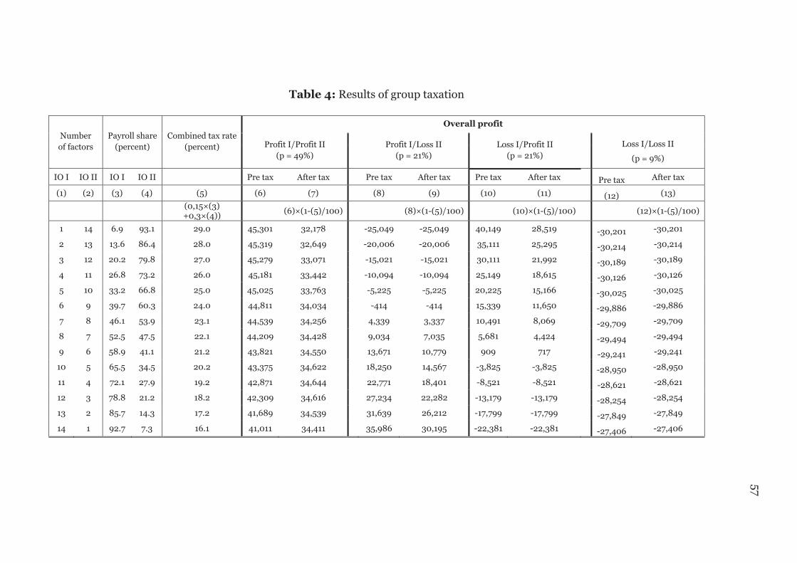
Table 4: Results of group taxation

Number

of factors

Payroll share

(percent)

Combined tax rate

(percent)

Overall profit

Profit I/Profit II

(p = 49%)

Profit I/Loss II

(p = 21%)

Loss I/Profit II

(p = 21%)

Loss I/Loss II

(p = 9%)

IO I IO II IO I IO II

Pre tax After tax Pre tax After tax Pre tax After tax Pre tax After tax

(1) (2) (3) (4) (5) (6) (7) (8) (9) (10) (11) (12) (13)

(0,15×(3) +0,3×(4))

(6)×(1-(5)/100)

(8)×(1-(5)/100)

(10)×(1-(5)/100)

(12)×(1-(5)/100)

1 14 6.9 93.1 29.0 45,301 32,178 -25,049 -25,049 40,149 28,519 -30,201 -30,201

2 13 13.6 86.4 28.0 45,319 32,649 -20,006 -20,006 35,111 25,295 -30,214 -30,214

3 12 20.2 79.8 27.0 45,279 33,071 -15,021 -15,021 30,111 21,992 -30,189 -30,189

4 11 26.8 73.2 26.0 45,181 33,442 -10,094 -10,094 25,149 18,615 -30,126 -30,126

5 10 33.2 66.8 25.0 45,025 33,763 -5,225 -5,225 20,225 15,166 -30,025 -30,025

6 9 39.7 60.3 24.0 44,811 34,034 -414 -414 15,339 11,650 -29,886 -29,886

7 8 46.1 53.9 23.1 44,539 34,256 4,339 3,337 10,491 8,069 -29,709 -29,709

8 7 52.5 47.5 22.1 44,209 34,428 9,034 7,035 5,681 4,424 -29,494 -29,494

9 6 58.9 41.1 21.2 43,821 34,550 13,671 10,779 909 717 -29,241 -29,241

10 5 65.5 34.5 20.2 43,375 34,622 18,250 14,567 -3,825 -3,825 -28,950 -28,950

11 4 72.1 27.9 19.2 42,871 34,644 22,771 18,401 -8,521 -8,521 -28,621 -28,621

12 3 78.8 21.2 18.2 42,309 34,616 27,234 22,282 -13,179 -13,179 -28,254 -28,254

13 2 85.7 14.3 17.2 41,689 34,539 31,639 26,212 -17,799 -17,799 -27,849 -27,849

14 1 92.7 7.3 16.1 41,011 34,411 35,986 30,195 -22,381 -22,381 -27,406 -27,406

57

Table 5a: Probability of additional subsequent payments for profit shifts from the group to an additional object

Shifted amount Probability of additional subsequent payment

(1) (2)

(1) × 0,0001

0 0

500 5

1,000 10

1,500 15

2,000 20

2,500 25

3,000 30

3,500 35

4,000 40

4,500 45

5,000 50

5,500 55

6,000 60

6,500 65

7,000 70

7,500 75

8,000 80

8,500 85

9,000 90

9,500 95

10000* 100

* Please note that the additional subsequent payment will be charged with certainty if the shifted amount is higher.

58

The CCCTB option – an experimental study

Claudia Keser, Gerrit Kimpel and Andreas Oestreicher

Appendix B: Regression Results

The CCCTB option – an experimental study 60 Table B.1: Choice of formula apportioment as the tax regime (Regression model 1)

Variables 1 = FA LCF at IO I -0.0999 (0.0954) LCF at IO II -0.371*** (0.0704) LCF at group level 0.239*** (0.0827) TD15 0.308 (0.253) Manager 0.0630 (0.265) Gender -0.313 (0.271) Business Experience -1.130*** (0.335) Risk level -0.0677 (0.0774) Time -0.00854* (0.00508) Period 0.0472*** (0.0124) Master 0.979*** (0.290) Impulsivity 0.134* (0.0807) Age -0.00417 (0.00910) Business Administration -0.446 (0.360) Economics -0.527 (0.396) Other Tax return prepared 0.408 (0.288) Constant -0.830 (0.675) Pseudo R2 0.280 Observation 982 Standard errors cluster robust Statistical significance at the 1%, 5% and 10% are denoted by ***, ** and *, respectively.

The CCCTB option – an experimental study 61 Table B.2: Allocation of production factors

Variables Overall SA FA LCF at IO I -0.0546 -0.0983* (0.0434) (0.0513) LCF at IO II 0.0231* 0.0249** (0.0126) (0.0119) LCF at group level 0.00957 0.0105 (0.0215) (0.0252) TD15 -0.343*** -0.240** -0.546*** (0.0933) (0.108) (0.147) Manager -0.126 -0.106 0.498*** (0.0860) (0.0777) (0.174) FA -0.237* (0.122) FA * Manager 0.595*** (0.169) Transfer to IO I 0.0256*** 0.0227*** (0.00532) (0.00446) Transfer to Z 0.0245*** 0.0325*** 0.0257*** (0.00568) (0.00786) (0.00877) Detection of transfer to IO I 0.00273 -0.0178 (0.0622) (0.0548) Detection of transfer to Z -0.0156 0.0392 -0.101 (0.0742) (0.0663) (0.138) Gender -0.0333 -0.0512 0.00769 (0.0926) (0.114) (0.149) Business Experience 0.0528 -0.0107 0.224 (0.124) (0.141) (0.268) Risk level -0.0338 -0.0431 0.0137 (0.0261) (0.0316) (0.0421) Time 0.00112 -0.000444 0.00380 (0.00106) (0.000965) (0.00239) Period 0.000146 0.00748 -0.0109 (0.00557) (0.00599) (0.0109) Master -0.108 -0.114 -0.175 (0.105) (0.134) (0.157) Impulsivity -0.0228 -0.0191 -0.0480 (0.0269) (0.0331) (0.0387) Age -0.0113*** -0.00767 -0.00861* (0.00350) (0.00540) (0.00494) Business Administration -0.0182 -0.116 0.262 (0.152) (0.134) (0.305) Economics 0.0948 0.108 0.180 (0.165) (0.142) (0.264) Other Tax return prepared -0.0145 0.00886 -0.127 (0.104) (0.101) (0.207) Constant 2.591*** 2.457*** 2.278*** (0.228) (0.259) (0.441) Lnalpha -1.495*** -1.943*** -1.172*** (0.273) (0.405) (0.387) Observation 1.245 738 507 Standard errors cluster robust cluster robust cluster robust Statistical significance at the 1%, 5% and 10% are denoted by ***, ** and *, respectively.

The CCCTB option – an experimental study 62 Table B.3: Profit shifts to IO 1

Variables LN profit shift to IO 1 LCF at IO I -0.127 (0.0863) LCF at IO II -0.256*** (0.0750) TD15 -1.265* (0.742) Manager 1.183* (0.669) Investment in IO II 0.127** (0.0498) Transfer to Z 0.0993 (0.158) Detection of transfer to IO I 0.713* (0.392) Detection of transfer to Z -1.134** (0.512) Gender -1.450** (0.736) Business Experience -1.719* (0.912) Risk level 0.386* (0.205) Time -0.00985 (0.00724) Period -0.0437 (0.0397) Master 2.403*** (0.791) Impulsivity 0.197 (0.221) Age 0.00849 (0.0352) Business Administration -0.971 (0.987) Economics -2.879** (1.133) Other Tax return prepared 0.785 (0.903) Constant 3.415 (2.102) R2 0.2645 Observation 738 Standard errors cluster robust Statistical significance at the 1%, 5% and 10% are denoted by ***, ** and *, respectively.

The CCCTB option – an experimental study 63 Table B.4: Profit shifts to the additional investment object Z

Variables LN transfer to Z

Overall SA FA LCF at IO I -0.110** -0.0875 (0.0516) (0.0556) LCF at IO II -0.146** -0.135* (0.0739) (0.0702) LCF at group level -0.262** -0.289** (0.123) (0.143) TD15 -0.642 -1.259* -0.118 (0.610) (0.655) (0.801) Manager 0.299 0.328 0.241 (0.573) (0.636) (0.813) FA 1.811*** (0.420) Transfer to IO I 0.0405 0.0600 (0.0396) (0.0451) Investment in IO II -0.00663 -0.0304 0.0187 (0.0313) (0.0420) (0.0389) Detection of transfer to IO I 0.0214 -0.151 (0.313) (0.306) Detection of transfer to Z 0.421 0.112 0.354 (0.298) (0.490) (0.398) Gender -1.179* -1.162 -0.972 (0.631) (0.723) (0.868) Business Experience 0.177 0.324 -1.992** (0.666) (0.757) (0.929) Risk level 0.336** 0.340* 0.0752 (0.160) (0.185) (0.203) Time -0.00910*** -0.00583 -0.0147* (0.00349) (0.00474) (0.00791) Period -0.00917 -0.0164 -0.0130 (0.0233) (0.0278) (0.0403) Master 0.158 0.996 -0.0592 (0.735) (0.950) (0.914) Impulsivity 0.283 0.0543 0.610** (0.196) (0.219) (0.291) Age 0.0240 0.0149 0.0259 (0.0305) (0.0429) (0.0273) Business Administration 0.277 -0.373 -0.744 (1.059) (1.323) (1.243) Economics 0.251 -1.129 0.126 (1.107) (1.330) (1.261) Other Tax return prepared 0.895 1.274 1.071 (0.753) (0.849) (1.175) Constant -0.207 1.996 1.501 (1.722) (2.121) (2.125) R2 0.1948 0.1789 0.2134 Observation 1.245 738 507 Standard errors cluster robust cluster robust cluster robust Statistical significance at the 1%, 5% and 10% are denoted by ***, ** and *, respectively.