the causes and consequences of land use regulation...

Journal of Urban Economics 65 (2009) 265–278

Contents lists available at ScienceDirect

Journal of Urban Economics

www.elsevier.com/locate/jue

The causes and consequences of land use regulation: Evidence from GreaterBoston ✩

Edward L. Glaeser a,b,∗, Bryce A. Ward a

a Harvard University, MA, USAb NBER, USA

a r t i c l e i n f o a b s t r a c t

Article history:Received 17 October 2006Revised 17 June 2008Available online 9 July 2008

Over the past 30 years, eastern Massachusetts has seen a remarkable combination of rising home pricesand declining supply of new homes, which doesn’t appear to reflect any lack of land. In this paper, weexamine the increasing number of land-use regulations in Greater Boston. These regulations vary widelyover space, and are hard to predict with any variables other than historical density levels. Minimumlot size and other land use controls are associated with reductions in new construction activity. Theseregulations are associated with higher prices when we do not control for contemporary density anddemographics, but not when we add these contemporaneous controls. These results are compatible witheconomic theory, which predicts that production restraints on a good won’t increase the price of thatgood relative to sufficiently close substitutes. Current density levels appear to be too low to maximizelocal land values.

© 2008 Elsevier Inc. All rights reserved.

1. Introduction

Over the past 25 years, many US cities have experienced a re-markable combination of increases in housing prices and decreasesin new construction (see Glaeser et al., 2005). Boston is an extremeexample of this phenomenon, with its dramatically rising housingprices. Table 1 shows that based on Office of Federal Housing En-terprise Oversight (OFHEO) repeat sales indices, three of the fourmetropolitan subdivisions with the greatest price appreciation be-tween 1980 and 2004 are in the Boston region (Boston–Quincy,Cambridge–Newton and Suffolk). At the same time, as Fig. 1 shows,the total number of permits issued in the Boston metropolitanarea declined from 172,000 during the 1960s, to 141,000 duringthe 1980s, to 84,000 during the 1990s.

The combination of rising prices and declining new supply sug-gests that Boston’s high prices reflect more than just rising de-mand. After all, without increasingly inelastic supply, an increasein demand should lead to higher prices and more construction.

✩ Glaeser thanks the Rappaport Institute for Greater Boston and the TaubmanCenter for State and Local Government for financial support. The data set was col-lected by the Pioneer Institute and we are particularly grateful to Amy Dain andJenny Schuetz for their work on the data. This paper partially incorporates earlierwork that was joint with Jenny Schuetz [Glaeser, E., Schuetz, J., Ward, B., 2006. Reg-ulation and the rise of housing prices in Greater Boston. Working paper. RappaportInstitute–Pioneer Institute]. David Luberoff provided significant assistance on thispaper.

* Corresponding author at: Harvard University, 1875 Cambridge Street, Cambridge,MA, USA.

E-mail address: [email protected] (E.L. Glaeser).

0094-1190/$ – see front matter © 2008 Elsevier Inc. All rights reserved.doi:10.1016/j.jue.2008.06.003

One natural hypothesis is that the supply of new housing in Bostonis falling because Greater Boston is running out of land. In Sec-tion 2 of this paper, we present evidence that seems to run counterto this hypothesis. Land densities are quite low in many areas ofBoston, and over the past 40 years, density has not risen signifi-cantly in the Boston area. Within the Boston region, higher densi-ties are associated with more, not less, permitting.

If increasing density levels cannot explain the decline in newconstruction, then one alternative hypothesis is that increasinglystringent land use regulations have made it more and more diffi-cult for developers to build (see Ellickson, 1977; Brueckner, 1990;and Glaeser et al., 2005). The primary contribution of this paperis to add results from a new data set on land use regulationsin Greater Boston to the literature that examines the impact ofland use restrictions on new construction and prices (see Maser etal., 1977; Katz and Rosen, 1987; Pollakowski and Wachter, 1990;Levine, 1999; Quigley and Raphael, 2005; and Ihlanfeldt, 2007).

Data on Greater Boston is a useful addition to these studiesbecause the area extensively uses land use controls, which are se-lected by particularly small towns that enjoy a great deal of controlover local building. Our data set gives us exceptionally detaileddata on the rules that localities have imposed on construction,which enables us to look at formal rules rather than more clearlyendogenous variables like the time delay involved in getting a per-mit. This data was collected by the Pioneer Institute for PublicPolicy Research and it contains information on the remarkable ar-ray of land use regulations in 187 cities and towns within GreaterBoston, including minimum lot sizes, wetlands regulations, septic

http://www.ScienceDirect.com/

http://www.elsevier.com/locate/jue

mailto:[email protected]

http://dx.doi.org/10.1016/j.jue.2008.06.003

266 E.L. Glaeser, B.A. Ward / Journal of Urban Economics 65 (2009) 265–278

Source. US Census Bureau.

Fig. 1. Total permits in Boston metro-area, 1961–2002.

Table 1Percent change in housing prices, 1980–2004, top 20 metropolitan areas.

Percent change in OFHEO repeat sales index,1980–2004

Percent change in OFHEO repeatsales index, 1980–2004 (%)

Nassau–Suffolk, NY Metropolitan Division 251Boston–Quincy, MA Metropolitan Division 210Cambridge–Newton–Framingham, MAMetropolitan Division

180

Essex County, MA Metropolitan Division 179Salinas, CA Metropolitan Statistical Area 162New York–Wayne–White Plains, NY–NJMetropolitan Division

158

Napa, CA Metropolitan Statistical Area 156Santa Cruz–Watsonville, CA MetropolitanStatistical Area

156

Worcester, MA Metropolitan Statistical Area 149San Luis Obispo–Paso Robles, CA MetropolitanStatistical Area

146

San Francisco–San Mateo–Redwood City, CAMetropolitan Division

138

San Jose–Sunnyvale–Santa Clara, CAMetropolitan Statistical Area

137

Santa Rosa–Petaluma, CA MetropolitanStatistical Area

131

Santa Barbara–Santa Maria–Goleta, CAMetropolitan Statistical Area

129

Providence–New Bedford–Fall River, RI–MAMetropolitan Statistical Area

129

Oakland–Fremont–Hayward, CA MetropolitanDivision

116

Edison, NJ Metropolitan Division 114Newark–Union, NJ–PA Metropolitan Division 112Oxnard–Thousand Oaks–Ventura, CAMetropolitan Statistical Area

109

San Diego–Carlsbad–San Marcos, CAMetropolitan Statistical Area

109

Source. OFHEO repeat sales index, raw index is adjusted for inflation using CPI mi-nus shelter.

rules and subdivision requirements.1 For many of the regulations,the data set also includes the dates when the regulations were im-posed, so it is possible to look at changes over time.

In Section 3 of the paper, we establish three basic facts aboutland use regulation in eastern Massachusetts. First, along most di-mensions there has been a dramatic increase in regulation since1980. For example, the share of communities with rules restrictingsubdivisions has increased from less than 50 percent in 1975 to al-most 100 percent today. Second, as Ellickson (1977) emphasized,there is a remarkable variety in the nature of these regulations:minimum lot sizes, subdivision rules, and septic and wetlands re-strictions that go significantly beyond the state standards are onlythe most basic of regulations. Third, land use regulations are oftenastonishingly vague, which increases the likelihood that there willbe disputes about implementation.

We then turn to the determinants of land use regulations. LikeEvenson and Wheaton (2003), we find that historical housing den-sity is the most important determinant of minimum lot size. Moremanufacturing and more minorities in 1940 are also associatedwith smaller minimum lot sizes. Septic and wetlands regulationsare associated with the historical presence of standing water. Theempirical exercise of trying to explain land use restrictions did notyield any explanatory variables that can satisfy the exclusion re-striction needed for them to be valid instruments for land usecontrols in a price or construction regression. Instead, we comeaway with the view that the bulk of these rules seem moderatelyrandom and unrelated to most obvious explanatory variables. Theabsence of good instruments and the seeming randomness of therules lead us to use the rules directly in our empirical work on theconsequences of land use regulations.

1 The database and a detailed discussion about how it was obtained is availableat http://www.masshousingregulations.com/.

http://www.masshousingregulations.com/

E.L. Glaeser, B.A. Ward / Journal of Urban Economics 65 (2009) 265–278 267

Source. US Census Bureau.

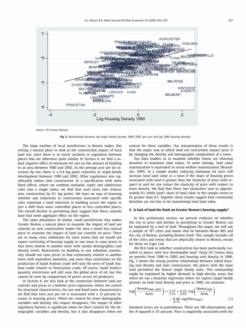
Fig. 2. Relationship between log single family permits 1980–2002 per acre and log 1980 housing density.

The large number of local jurisdictions in Boston makes thissetting a natural place to look at the construction impact of localland use, since there is so much variation in regulation betweenplaces that are otherwise quite similar. In Section 4, we find a ro-bust negative effect of minimum lot size on the amount of buildingin an area between 1980 and 2002. As the average acre per lot in-creases by one, there is a 0.4 log point reduction in single-familydevelopment between 1980 and 2002. Other regulations also sig-nificantly reduce new construction. In a specification with townfixed effects, where we combine wetlands, septic and subdivisionrules into a single index, we find that each extra rule reducesnew construction by 0.1 log points. We have no way of knowingwhether any reductions in construction associated with specificrules represent a total reduction in building across the region orjust a shift from more controlled places to less controlled places.The overall decline in permitting does suggest that these controlshave had some aggregate effect on the region.

The same abundance of similar, small jurisdictions that makesGreater Boston a natural place to examine the impact of land usecontrols on new construction makes the area a much less naturalplace to examine the impact of land use controls on price. Thereare so many close substitutes for most towns that we would notexpect restricting of housing supply in one town to raise prices inthat town relative to another town with similar demographics anddensity levels. Restrictions on building in one suburban commu-nity should not raise prices in that community relative to anothertown with equivalent amenities, any more than restrictions on theproduction of Saudi Arabian crude will raise the price of Saudi Ara-bian crude relative to Venezuelan crude. Of course, Saudi Arabia’squantity restrictions will still raise the global price of oil, but thiscannot be seen by comparisons of prices across oil producers.

In Section 4, we also look at the connection between land usecontrols and prices in a hedonic price regression, where we controlfor structural characteristics, lot size and fixed town characteristics,we find that each acre per lot is associated with a 12 percent in-crease in housing prices. When we control for town demographicvariables and density, this impact disappears. The impact of otherregulatory barriers is significant when we don’t control for the de-mographic variables and density, but it also disappears when we

control for these variables. Our interpretation of these results isthat the major way in which land use restrictions impact price isby changing the density and demographic composition of a town.

Our data enables us to examine whether towns are choosingdensities to maximize land values. In some settings, land valuemaximization is equivalent to social welfare maximization (Brueck-ner, 1990). In a simple model, reducing minimum lot sizes willincrease total land value in a town if the share of housing pricesassociated with land is greater than the elasticity of price with re-spect to unit lot size minus the elasticity of price with respect totown density. We find that these two elasticities sum to approxi-mately 0.1, while land’s share of total value in the sample seems tobe greater than 0.5. Together these results suggest that communitydensities are too low to be maximizing total land value.

2. Is lack of land the limit on Greater Boston’s housing supply?

In this preliminary section, we present evidence on whetherthe rise in price and decline in permitting in Greater Boston canbe explained by a lack of land. Throughout this paper, we will usea sample of 187 cities and towns that lie between Route 495 andthe city of Boston, excluding Boston itself. This sample includes allof the cities and towns that are physically closest to Boston, exceptfor those on Cape Cod.

We first look at whether construction has been particularly cur-tailed in places with less developable land. Using US Census dataon permits from 1980 to 2002 and housing unit density in 1980,Fig. 2 shows the strong positive relationship between initial hous-ing unit density and later construction; the places with the mostland permitted the fewest single family units. This relationshipmight be explained by higher demand in high density areas, butwhen we run a bivariate regression where we regress single familypermits on both land density and price in 1980, we estimate:

Log

(Permits1980–2002

Acres

)= 3.27

(1.53)+ 0.22

(0.03)·Log

(Homes1980

Acres

)

− 0.46(0.13)

·Log(Price1980). (1)

Standard errors are in parentheses. These are 186 observations andthe R-squared is 55 percent. Price is negatively associated with the


amount of development, which again suggests the importance oflimits on supply, for otherwise there would surely be more build-ing in the areas where demand is stronger. Controlling for initialprice has virtually no impact on the relationship between con-struction and initial density, which remains quite positive. How canlack of land be driving the reduction in permits if there is the leastconstruction in areas with the most land?

A second piece of evidence supporting the view that declin-ing construction levels don’t reflect a lack of land is the existenceof many towns with the combination of high prices, low densitylevels and low levels of new construction. Lincoln, Weston andConcord are three contiguous towns that illustrate low levels ofconstruction in land rich areas. Together, they have 12,889 homesand cover more than 39,000 acres. Yet despite being among themost expensive towns in the state, these areas together permit-ted just 1746 new homes, or less than 0.045 new homes per acre,between 1980 and 2002. In our sample of 187 towns, there are an-other 22 localities with less than one home for every two acresthat have allowed less than 30 units per year each since 1980.2

A third piece of evidence, running counter to the view thatGreater Boston is running out of land, is that density levels havenot increased very much over the past 25 years. For example, thetotal housing density in Suffolk County (which contains Boston) in-creased by 4.5 percent in the 1970s, 4.6 percent in the 1980s and1.1 percent in the 1990s. Middlesex County (which contains Cam-bridge) grew more, but even its housing unit density increased byonly 10.3 percent in the 1980s and by 6 percent in the 1990s.

Can such modest increases in density explain the reduction inthe number of new units permitted? One approach to answeringthis question is to run a panel regression where an observation isa town-year. If we do not control for density, but do control fortown fixed effects, we estimate that construction falls by −0.267log points after 1990 (the standard error is 0.05). We use a post-1990 dummy variable because it is a simple and convenient wayto empirically capture the decline in permitting intensity, not be-cause there is anything special about that year. If we just controlfor density in the panel regressions (removing town fixed effects),then the estimated decline in permitting increases, since density ispositively predicted with new permits and density is rising.

Alternatively, we can fix the coefficient on density in these re-gressions at different values and see how much this reduces thereduction in permitting over time. For example, if we fix to thecoefficient on density as −0.1, which reflects a national regressionrun by Glaeser et al. (2005), then the estimated dummy variableon the 1990s falls in absolute value to −0.25. If we fix the coef-ficient on density at −0.25, the estimated dummy variable on the1990s is −0.23. This is a large coefficient on density, and even withsuch a large coefficient, density can only explain 14 percent of thedecrease in eastern Massachusetts construction in the 1990s.

A fourth piece of evidence that runs counter to the view thatdeclining construction levels reflect a lack of land is that land isnot particularly valuable in housing price hedonic regressions. Ifland use restrictions didn’t exist, then in equilibrium, land that ex-tends a lot would be worth the same as land that sits under a newlot (see Glaeser and Gyourko, 2003). Using data from Banker andTradesman from 2000 to 2005, we estimate a standard hedonic re-gression with structural characteristics and find that an extra acreof land is associated with an extra cost of only $16,000. This isnot a high value of land, given that the average home sales price is

2 Overall, between 1980 and 2002, the total amount of permits was 313,762 unitsspread over 2,180,795 acres, or 0.14 new homes per acre.

$450,000, which is approximately $270,000 more than the physicalcost of building an average unit in Boston.3

Since the average home in our sample sits on 0.7 acres, a back-of-the-envelope calculation suggests that an acre is worth morethan 300,000 dollars if it sits under a new home, but less than20,000 dollars if it extends an existing lot. The mismatch betweenthose two numbers suggests that Boston cannot be understood asa market where land is scare and land use is unrestricted. In thatcase, the value of an acre should be the same if it extends an ex-isting lot or is used to create a new lot.

A final piece of evidence on the land shortage hypothesis is thatlot sizes for new homes in the Boston area rose from 0.76 in 1990to 0.91 in 1998 (Jakabovics, 2006). Rising lot sizes are hard to rec-oncile with a land shortage. One explanation of this phenomenonis that incomes were rising, but Glaeser et al. (2008) estimate anincome elasticity of demand for land among single-family home-owners of less than 0.2 and Boston area income rose by less thanfive percent. Those estimates predict a one percent increase in av-erage lot size, not the 20 percent increase that is actually observed.

3. Data description and the causes of land use regulation

The combination of increasing prices and decreasing construc-tion can’t be explained by a lack of land, but perhaps it can beexplained by a man-made land shortage created by an increas-ingly stringent regulatory environment. To consider this possibil-ity, we now turn to the Pioneer Institute’s Housing RegulationDatabase for Massachusetts Municipalities in Greater Boston. Thisdata was assembled by a team of researchers who interviewed lo-cal officials about the rules facing local developers. This data wassupplemented with data from the MassGIS system which detailsfor 1999–2000 the minimum lot size requirements throughout thestate.4 Our permitting and demographic data come from the Cen-sus.

3.1. Minimum lot sizes

Before turning to the non-lot regulations, we will begin withthe basic facts about lot size requirements in eastern Mas-sachusetts. Lot sizes are not uniform within most towns; thereare generally several different planning sub-areas. We include allsub-areas where it is possible to build single family housing. Sinceour permitting and price information is at the town level, we ag-gregate sub-area data on minimum lot size using the formula:

LotSizeMinimum = TotalTownLandArea∑Sub-areas

LandAreaMinimumLotSize

. (2)

The formula essentially divides the total land area in the town bythe number of homes that can be built in the town. The denomi-nator calculates the total units that could be built in the town bysumming across areas the total number of units that could be builtin each sub-area, or LandArea

MinimumLotSize .The effect of minimum lot size should be particularly striking

on undeveloped land, but since Greater Boston is one of America’soldest urban areas, there is extremely little truly undeveloped landwithin the region. The impact of lot sizes in this region shouldwork primarily by reducing the ability to subdivide existing prop-erties, which is why we look at minimum lot sizes throughout thetown.

There is a great deal of variation in this variable across our 187cities and towns. One-fifth of the population and slightly under

3 Gyourko and Saiz (2006) estimate that the cost of construction is less than100 dollars per square foot in Boston and the average home in our sample is 1800square feet.

4 This system was used and described more thoroughly by Evenson and Wheaton(2003).


Table 2Characteristics of municipalities, by average SF minimum lot size.

(1) (2) (3) (4)Mean SF minimum lot size

<20,000 20–35,000 35–50,000 50,000+Share of regional pop. 42.7 21.7 21.3 14.3Share of regional land 12.7 18.9 28.8 39.6Number of towns 42 38 51 55Mean population 41,338 23,218 16,987 10,571

[32,007] [17,385] [12,477] [7851]Pct. white 84.5 92.1 93.7 94.5

[15.1] [7.9] [3.8] [4.1]Pct. foreign-born 13.9 7.2 6.2 5.3

[8.5] [4.9] [2.9] [3.2]Pct. w/BA+ 37.3 35.2 38.8 43.1

[17.6] [13.6] [14.6] [19.2]Distance to Boston (miles) 14 22 24 28

[10] [8] [8] [8]Land area (acres) 6551 10,829 12,254 15,642

[5240] [4651] [5218] [9742]Pct. housing in SF 49.6 68.3 73.5 79

[21.9] [16.5] [12.4] [13.5]Mean hsg price 238,160 217,818 229,635 265,444

[91,766] [73,394] [74,562] [124,045]Mean rent 829 732 714 773

[159] [166] [121] [202]

Source. US Census, MassGIS.

one-tenth of the towns have average lot sizes of 10,000 feet orless (one quarter acre), while slightly under one-tenth of the townshave average lot sizes of 70,000 feet or more. Unsurprisingly, peo-ple tend to live disproportionately in areas with denser zoning andland tends to be disproportionately allocated to less dense zoning.Towns are particularly likely to have between 30,000 and 40,000foot minimum lot size, which is about one acre, and which is alsothe average lot size of new homes found by Jakabovics (2006).

In Table 2, we show the distribution of town characteristicsby minimum lot size broken into four categories. The towns withsmaller minimum lot sizes are larger, with populations that aremore likely to be non-white and foreign born. The towns withlarger lot sizes are further from Boston, and have higher housingprices when we do not use controls. Income and education levelsare mildly higher in the areas with high minimum lot sizes.

3.2. Other land use regulations

While minimum lot size is the single most important land-use regulation, Massachusetts cities and towns have increasingly

adopted other rules that also impact new construction. The bulkof these rules make new development more difficult, but somerules—like cluster zoning—can make it easier to build. The PioneerInstitute survey categorized all of these rules across the 187 citiesand towns.

The three largest categories of added constraints on land usecontrols concern wetlands, septic systems and subdivision require-ments. Both wetlands and septic systems are also regulated at thestate level, but our focus is on the town level rules that go be-yond the state’s regulations. While a majority of towns have gonebeyond the state standards, there is considerably heterogeneity intown-level regulations.

For example, the state Wetlands Protection Act protects all landwithin 100 feet of a wetland or floodplain, which includes all landthat has 10,890 cubic feet of standing water at least once per year.Of the 131 communities that have imposed wetlands regulationsthat go beyond the state standard, 59 of them have introducedmore stringent definitions of floodplains. Eleven of them, for ex-ample, have defined floodplains as including all areas that have5445 cubic feet of standing water. A number of them have goneto 1000 cubic feet of standing water or less. Twenty-four of thesecommunities have adopted amorphous verbal definitions of flood-plains, such as “an isolated depression. . . that confines standingwater” (see Dain, 2006).

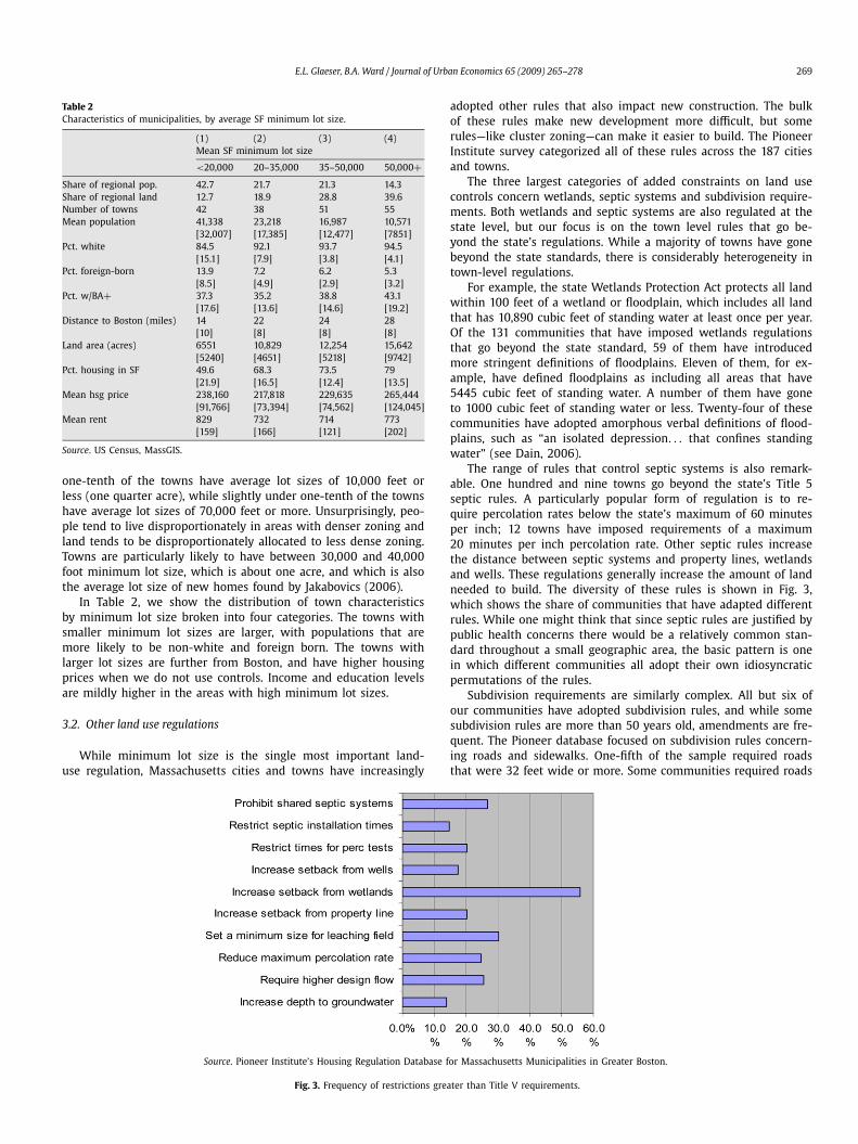
The range of rules that control septic systems is also remark-able. One hundred and nine towns go beyond the state’s Title 5septic rules. A particularly popular form of regulation is to re-quire percolation rates below the state’s maximum of 60 minutesper inch; 12 towns have imposed requirements of a maximum20 minutes per inch percolation rate. Other septic rules increasethe distance between septic systems and property lines, wetlandsand wells. These regulations generally increase the amount of landneeded to build. The diversity of these rules is shown in Fig. 3,which shows the share of communities that have adapted differentrules. While one might think that since septic rules are justified bypublic health concerns there would be a relatively common stan-dard throughout a small geographic area, the basic pattern is onein which different communities all adopt their own idiosyncraticpermutations of the rules.

Subdivision requirements are similarly complex. All but six ofour communities have adopted subdivision rules, and while somesubdivision rules are more than 50 years old, amendments are fre-quent. The Pioneer database focused on subdivision rules concern-ing roads and sidewalks. One-fifth of the sample required roadsthat were 32 feet wide or more. Some communities required roads

Source. Pioneer Institute’s Housing Regulation Database for Massachusetts Municipalities in Greater Boston.

Fig. 3. Frequency of restrictions greater than Title V requirements.


Source. Pioneer Institute’s Housing Regulation Database for Massachusetts Municipalities in Greater Boston. Communities who adopt provi-sions at unknown dates are excluded from fraction.

Fig. 4. Fraction of communities with wetlands, septic, subdivision, and cluster provisions, 1975–2004.

that were 22 feet wide or less. There are also restrictions on side-walks and curb materials.

Rules regarding lot shape also restrict subdivisions. Sometimesthese rules are straightforward requirements that restrict the ratioof perimeter to area. In other cases the rules are more amorphous,such as the town of Millbury’s prohibition that “No pork chop,rattail, or excessively funnel-shaped or otherwise gerrymanderedlots shall be allowed.” Fifty-four towns have also instituted growthmanagement policies that just act as a brake on the amount ofnew development.

There are three sets of policies that enable developers to avoidthe minimum lot size regulations. First, a large number of com-munities have adopted cluster zoning, which enables builders touse smaller lot sizes in exchange for setting aside some quantityof open space. In many cases, cluster zoning doesn’t actually havea density bonus, because the open space set aside must be enoughso that the total density of the lot size still conforms to existingminimum lot size rules. Inclusionary zoning can enable developersto avoid minimum lot size requirements if they include enough af-fordable units. Towns have an incentive to build these affordableunits, because if they have too few units, developers can use thestate rule Chapter 40B, which allows them to ignore local zoningordinances. Still, we have only found 21 towns where builders havetaken advantage of inclusionary zoning rules. A third set of rulesallow builders to develop at higher densities if the units are re-stricted to the elderly.

In our empirical work, we will use a simple categorical variablethat takes on a value of one if the town has passed a rule that goesbeyond the state standards regarding septic systems, wetlands andsubdivisions. We will also sum those three categorical variables to-gether for an overall regulatory barriers index (similar to Quigleyand Raphael, 2005). While there is surely information lost in us-

ing such a coarse measure, the advantage of such coarseness isthat it provides a simple measure with limited opportunities fordata mining. This metric attempts to capture the overall regula-tory environment in each community, while avoiding the loss ofstatistical clarity associated with trying to look at the effects ofall three regulations simultaneously. As Pollakowski and Wachter(1990) argue, “land-use constraints collectively have larger effectsthan individually.” We also examine the impact of cluster and in-clusionary zoning.

Fig. 4 shows the adoption levels of the three forms of regula-tory barriers and cluster zoning. All forms of regulation show adramatic increase over time. The subdivision rules have now be-come ubiquitous. Fig. 5 shows the share of communities that haveamended their wetland, cluster and subdivision bylaws by year.There was a dramatic increase in the end of the 1990s. These in-creases were also accompanied by an increasing use of the courtsystem by the opponents of growth. Lawsuits, particularly justifiedon environmental or nuisance grounds are also a perennial devel-oper’s complaint. Fig. 6 shows the results of a Lexis/Nexis search ofMassachusetts Court Decisions containing all of the keywords zon-ing, residential and either septic or wetland from 1964 to 2004.Again, there was a steady rise in the 1990s.

3.3. The causes of land use regulation

We now turn to the correlates of these regulations by regress-ing these rules on variables that predate the rules enactment. Weknow when the wetlands, septic and subdivision regulations wereput in place, but we do not have comparable data for minimumlot sizes. However, we do know that there was an initial waveof zoning in the 1920s followed by a much greater wave afterWorld War II. As such, 1915 characteristics can be thought of as


Source. Pioneer Institute’s Housing Regulation Database for Massachusetts Municipalities in Greater Boston.

Fig. 5. Number of communities amending wetlands bylaws, subdivision rules, and cluster provisions, 1984–2004.

Source. Lexis–Nexis.

Fig. 6. Massachusetts Court Decisions containing keywords: Zoning, residential and septic or wetland, 1964–2004.

pre-dating minimum lot size rules for all of the towns, and 1940characteristics will predate minimum lot sizes for most of the ar-eas.

Table 3 first looks at the correlation between minimum lotsizes and 1915 town characteristics. Missing data from the earlycensuses causes us to lose a small number of cities. The most sig-

nificant variable is density in 1915. As density increases by one logpoint, current minimum lot size decreases by about one-quarteracre. In regression (2), we show results using 1940 data. In thiscase, the impact of density in 1940 is quite similar. On its own,density in 1940 can explain 68 percent of the variation in cur-rent minimum lot sizes. As such, we can basically interpret current


Table 31915, 1940 determinants of average minimum lot size and 1970 determinants of wetland bylaws, septic rules, and cluster zoning.

(1)Average minimum

(2)Lot size

(3)Wetland bylaws

(4)Septic rules

(5)Cluster provisions

ln(Town Area) 0.0152 0.0108 −0.0592 −0.1811 0.1803[0.0490] [0.0394] [0.1098] [0.1726] [0.0959]

ln(Housing Density) −0.2425 −0.2683 0.0371 −0.3849 0.1259[0.0269]** [0.0209]** [0.0551] [0.0846]** [0.0470]**

Distance to Boston 0.0027 −0.0029 −0.002 −0.0085 0.0032[0.0027] [0.0024] [0.0050] [0.0065] [0.0039]

Pct. white −0.0129 0.0086 0.0066 −0.048 −0.009[0.0108] [0.0086] [0.0233] [0.0471] [0.0191]

Pct. foreign born −0.0063 −0.005 −0.0284 −0.0202 −0.0119[0.0032] [0.0048] [0.0183] [0.0271] [0.0148]

Pct. mfg −0.0652 −0.1917[0.1590] [0.0962]*

Pct. owner occupied −0.0064 −0.0016 −0.0037 −0.0016[0.0019]** [0.0040] [0.0056] [0.0031]

Pct. BA or higher 0.0076 0.0053 0.0078[0.0041] [0.0055] [0.0034]*

ln(acres water-based recreation + 1) 0.0615 0.0868 −0.0126[0.0253]* [0.0341]* [0.0196]

ln(acres water + wetlands + 1) 0.0414 0.1643 0.0492[0.0554] [0.0820]* [0.0468]

ln(acres of new development 1971–1985 + 1) 0.1104 0.0956 0.0203[0.0524]* [0.0846] [0.0393]

Constant 3.0573 −0.1748[1.2204]* [0.9382]

Control year 1915 1940 1970 or 1971 1970 or 1971 1970 or 1971Observations 185 182 186 186 186R-squared 0.64 0.71

Notes. (1) Standard errors in brackets.(2) Dependent variable for (1) and (2) is average minimum lot size. Dependent variable for (3), (4) and (5) is a 0/1 variable indicating the existence of the regulation.

Standard errors are clustered at the town level for regressions (3), (4) and (5).(3) Data is from the Pioneer Institute’s Housing Regulation Database for Massachusetts Municipalities in Greater Boston at http://www.masshousingregulations.com/,

MassGIS, the Harvard Forest Survey of Massachusetts and the US Census Bureau.* Significant at 5%.

** Significant at 1%.

rules as enforcing the level of density that was in place almost acentury ago.

Other town characteristics are also correlated with minimumlot sizes, but the effects are much weaker. There is also a modestnegative correlation between share of the population that worksin manufacturing in 1940 and less restrictive minimum lot sizes.The same correlation appears in 1915, but the coefficient is statis-tically insignificant. There are two plausible explanations for thisphenomenon. First, manufacturing may proxy for working classresidents who were less concerned with restricting building forthe poor. Second, manufacturing may proxy for the presence ofbusinesses that have an interest in building more to keep housingprices low so that they don’t need to pay workers more to com-pensate them for high housing costs.

Percent white in 1940 is associated with slightly more stringentminimum lot sizes. This result does not appear in 1915 becausethere is almost no variation in percent white during that year. The1915 parallel is that towns with more immigrants have less strin-gent minimum lot sizes. These results present weak evidence forthe view that high minimum lot sizes where used by white na-tives to restrict homes built for blacks and foreigners. It is alsouseful to note the variables that don’t matter. For example, dis-tance to Boston is irrelevant once we control for housing density.The share of homeowners in the town is actually associated withless restrictive zoning, but this effect is quite weak.

The connection between historical density and minimum lotsizes prompted us to look for more ancient causes of minimum lotsizes. Using data from the Harvard Forest Survey of Massachusetts,we regressed minimum lot size today on the share of the townthat was forested in 1885. There is a 52 percent correlation be-tween this variable and minimum lot size, which is shown in Fig. 7.Forest cover in most of those towns in the 19th century was deter-

mined by the value of agricultural land, so it reasonable to thinkthat current zoning patterns reflect, in part, whether a town wasworth clearing and settling based on the value of its pre-modernagricultural productivity.

We now turn to the determinants of these land use regulations.Since subdivision requirements are so ubiquitous, we exclude thoseand focus on whether the town has wetlands rules, septic rulesand cluster zoning. We include 1970 controls that predate theseregulations. The results are shown in regressions (3), (4) and (5)of Table 3, which presents the marginal effects from probit regres-sions. While we have included a rich bevy of controls, almost noneof these controls actually explain the adoption of these rules. Thisis not because we have included a large number of controls, asalmost nothing is consistently, significantly correlated with theseoutcomes when fewer controls are included.

In the case of wetlands regulation, the variable that most re-liably and significantly predicts wetlands rules is the amount ofrecreation water in the township. Places with more recreationalwater are unsurprisingly more dedicated to protecting wet spaces.They are also more likely to regulate septic systems more strin-gently. Septic rules are particularly negatively associated with highlevels of housing density, if high density places are more likely torely on sewers rather than septic tanks.

We were surprised that so few of the other variables were sta-tistically significant. In the case of wetlands restrictions, there is asignificant positive relationship between the amount of new devel-opment in the 70s and early 80s and adoption, and a marginallysignificant positive relationship between adoption and the share ofthe population with 16 years or more of schooling. More gener-ally, these regulations which vary so much from town to town, aresurprisingly uncorrelated with most town characteristics. This mayeither reflect an efficiency view of these regulations where they



Source. MassGIS, Harvard Forest Archive.

Fig. 7. Relationship between minimum lot size and forested area 1885.

are being tied to un-measured land characteristics or the view thatthese regulations are fairly random.

In the third regression, we look at the correlates of cluster zon-ing. In this case, bigger and denser towns are much more likely tohave cluster zoning, presumably because those residents are lesstroubled by the occasional denser development. There is also aweak correlation with education levels which may reflect the factthat “Smart Growth” has become popular among environmentallyoriented educated elites.

These results do not lead us towards any natural instrumentsfor land use regulations. While historical density may be a rea-sonable instrument for total current density, it cannot be used toseparately identify the impact of land use controls, since historicaldensity is likely to have a direct impact on the amount of build-ing in an area and prices.5 Likewise, the presence of recreationalwater seems likely to impact prices directly because that water issurely an amenity. We take these regressions as suggesting that, atleast when controlling for historical density, the regulations seemunpredictable enough that we are comfortable using them directlyin our regressions on the consequences of land use controls.

4. The consequences of land use regulation

We now turn to the consequences of land use regulation. Wefirst look at permitting and then turn to prices. The permittingresults can only tell us whether regulations are associated witha reduction in permitting in one jurisdiction relative to another,and cannot tell us the area-wide impact of permitting. As we willdiscuss later, there are reasons to doubt that price level regressions

5 The use of historic density, and other demographic variables, as instruments forcurrent zoning, which is the approach used by Ihlanfeldt (2007), offers the possi-bility of reducing the endogeneity problem of zoning rules. However, changes indemographics over time also seem quite likely to be related to unobserved arealevel characteristics. In that case, in a regression that controls for current demo-graphics, past demographics may not satisfy the needed exclusion restriction.

will find an effect of permitting on price, at least if we control fullyfor other area wide characteristics.

We begin with minimum lot size and then turn to the otherregulations. In the case of minimum lot size, we can only look atthe cross section of towns, since we do not know when these ruleswere adopted. Our basic specification is to regress:

Log(Permits) = α · LotSizeMinimum + TownCharacteristics, (3)

where permits represents the total number of permits issued overthe relevant time periods (the 1980s, the 1990s and the entire1980–2002 period). We will primarily focus on single family per-mits, but also present results for total permits. The results of theseregressions can be found in Table 4.

For the regressions that include permits from the 1980s, ourtown controls include the logarithm of town area, distance toBoston, the logarithm of the housing stock in 1980, the share ofthe population that is less than 18 years old in 1980, the percentof the adult population with a college degree in 1980 and the per-cent white in 1980. We also include a dummy variable for whetherthe town has a major university, which we define as being amongthe top 50 universities or top 25 colleges in the 2005 US News andWorld Report rankings. For the regressions that look at permits inthe 1990s, we use controls from the 1990 Census.

The first three regressions look at results for single family per-mits for 1980–2002 and for the 1980s and 1990s separately. Thecoefficient for the whole period is −0.4 which has a t-statistic of2.9. The coefficient in the 1980s is also −0.4 and the coefficient inthe 1990s is −0.36. The changes across specifications are too smallto have any statistical meaning. These coefficients should be inter-preted as suggesting that as the town increases the average lot sizeneeded to build by one acre, the number of new permits declinesby −0.4 log points or about 40 percent.

Several of the variables also reliably predict new construction.For example, the logarithm of town area has coefficient between0.8 and 0.96, which suggests that the elasticity of permitting withrespect to total land area is close to one. The coefficient on thehousing stock in 1980 is also strongly positive, which gives us that


Table 4Effect of minimum lot size on permits and housing stock, 1980–2002.

(1) (2) (3) (4) (5) (6)ln(total single family permits) ln(total permits)

1980–2002 1980–1989 1990–1999 1980–2002 1980–1989 1990–1999

Acres per lot −0.3982 −0.402 −0.361 −0.3085 −0.3123 −0.3384[0.1392]** [0.1541]** [0.1696]* [0.1346]* [0.1559]* [0.1642]*

Log of Town Area 0.8498 0.7907 0.9367 0.7028 0.5834 0.9056[0.0892]** [0.0987]** [0.1101]** [0.0884]** [0.1023]** [0.1138]**

Distance to Boston 0.0057 0.0053 0.0046 −0.0043 −0.0057 0.0014[0.0050] [0.0055] [0.0058] [0.0047] [0.0055] [0.0057]

Major university 0.048 0.0897 −0.4595 0.1303 −0.0212 −0.3603[0.2306] [0.2552] [0.2773] [0.2168] [0.2510] [0.2633]

Log of Housing Stock (Initial period) 0.3105 0.3615 0.365 0.4205 0.5336 0.3863[0.0745]** [0.0824]** [0.0968]** [0.0769]** [0.0890]** [0.1032]**

Pct. <18 (Initial period) 0.0498 0.0428 0.0595 0.0447 0.0369 0.0506[0.0128]** [0.0142]** [0.0179]** [0.0133]** [0.0154]* [0.0176]**

Pct. BA+ (Initial period) −0.0044 −0.0032 −0.0005 −0.0071 −0.0099 0.0007[0.0031] [0.0035] [0.0033] [0.0033]* [0.0038]** [0.0034]

Pct. white (Initial period) 0.0183 0.0052 0.0374 0.0299 0.0187 0.0253[0.0124] [0.0137] [0.0087]** [0.0131]* [0.0151] [0.0090]**

Share of single family housing (1980) −0.0086 −0.006 −0.0049[0.0032]** [0.0037] [0.0036]

Constant −6.5124 −5.7276 −10.5979 −5.9161 −5.2229 −8.607[1.4627]** [1.6188]** [1.3023]** [1.4615]** [1.6920]** [1.2536]**

Observations 185 185 185 185 185 185R-squared 0.69 0.62 0.66 0.71 0.68 0.65

Notes. (1) Standard errors in brackets.(2) Dependent variable for regressions (1)–(3) is the ln(single permits) for the years indicated above, and the dependent variable for regressions (4)–(6) is the ln(total

permits) for the years indicated above.(3) Data from US Census Bureau, MassGIS, and the 2005 US News and World Report college and university rankings.

* Significant at 5%.** Significant at 1%.

places with more housing in 1980 have built more since then.6

Major universities are negatively correlated with development inthe 1990s, but not before then. Percent white is positively corre-lated with development in the 1990s. Towns with lots of youngpeople built more across both time periods.

In regressions (4)–(6), we turn to the logarithm of total permits.In this case, we also control for the initial share of the housingstock that is multi-family in an attempt to control for any long-standing tendencies to build high rise buildings. In this case, thecoefficient falls to −0.3 over the entire sample. The coefficient isslightly higher for the two other time periods.7 Overall, acres perlot is negatively associated with permitting in all of our specifica-tions and the coefficients are always statistically significant.

We can also look at the relationship between acres per lot andtotal housing density in 2000, controlling for housing density in1940. A simple regression across 187 cities and towns estimates:

Log

(Homes2000

Acres

)= 0.51

(0.03)·Log

(Homes1940

Acres

)

− 0.36(0.08)

·LotSizeMinimum + OtherControls. (4)

The other controls include distance to Boston, the presence of amajor university and the log of land area in the town. Standarderrors are in parentheses. As the acres per lot increases by one, thelogarithm of housing units in 2000 falls by 0.36 log points, whichcan be interpreted as suggesting a reduction of housing growth bythirty six percent over the entire 1940–2000 time period.

6 Controlling for the housing stock in 1980 is essentially controlling for the impactthat land use controls have had on building prior to that point. If we control insteadfor housing density in 1940, the coefficient on acres per lot rises in magnitude toapproximately −0.5.

7 While the effect of acres per lot is somewhat weaker on overall permitting thanit is on single family permitting, this change does not imply that acres per lot ispositively correlated with multi-family permits. Acres per lot is also negatively as-sociated with multi-family permits if those permits are treated separately.

Table 5 provides results for our other regulatory measures.Since we know when these regulations were imposed and sincewe have permits by year, we are now able to run panel regressionsboth with and without town fixed effects. When we exclude townfixed effects we include 1970-era controls, as we did in the regres-sion explaining these variables, which includes town area, housingstock, share of the population below age 18, share of the popula-tion that is white and share of the population with college degrees.We also include the dummy variable indicating the presence of amajor university. All standard errors are clusters by town.

The first two regressions show the three types of rules includedsimultaneously. In the specification with town controls, wetlandsand subdivision rules are negatively but insignificantly correlatedwith development. Septic rules are extremely weakly positively as-sociated with development. In the specification with town fixedeffects, all three coefficients negatively predict development, butonly the subdivision rules are statistically significant.

In regressions (3) and (4), we aggregate these variables intoan index by just adding them together. In the specification with-out fixed effects, the coefficient is −0.067, which is statisticallyinsignificant. In the specification with town fixed effects, the coef-ficient rises to −0.11 which has a t-statistic of two. This specifi-cation suggests that each new regulation is associated with abouta ten percent reduction in new construction. Of course, we cannotbe sure that these restrictions are actually causing the reductionin new construction. The decline in new construction might reflecta general anti-growth atmosphere that reflects itself in both newregulations and a reduction in permits.8

The estimated coefficient of −0.1 suggests new constructionfalls by about ten percent with each new regulation. We think thisestimated effect is fairly large. However, since the variation in newpermitting is also quite large, the estimate remains imprecise. This

8 Alternative ways of defining indices tended to yield broadly similar results.


Table 5Effect of additional zoning on annual total permits, 1980–2002.

(1) (2) (3) (4) (5) (6)ln(total permits)

Wetlands bylaw −0.055 −0.092[0.0737] [0.0856]

Septic rule 0.0559 −0.0117[0.0973] [0.1023]

Subdivision rule −0.1488 −0.2196[0.0924] [0.0974]*

Combined regulation index −0.0668 −0.1094 −0.0745 −0.14[0.0494] [0.0526]* [0.0604] [0.0677]*

Cluster 0.2408 0.1137[0.1062]* [0.1066]

Inclusionary 0.251 0.0449[0.1392] [0.1386]

Constant −10.9794 3.5201 −10.9199 3.4646 −9.9282 3.4665[1.1458]** [0.0862]** [1.1314]** [0.0780]** [1.1940]** [0.1042]**

Town controls Yes No Yes No Yes NoTown FE No Yes No Yes No YesYear FE Yes Yes Yes Yes Yes YesObservations 2507 2530 2507 2530 1732 1755R-squared 0.49 0.64 0.48 0.63 0.51 0.65

Notes. (1) Robust standard errors in brackets.(2) Standard errors are clustered on town.(3) Dependent variable is ln(total permits) in each year for 1980–2002.(4) Town controls include minimum lot size, ln(town area), ln(hsg 1980), major university dummy, pct. < 18 1980, pct. white 1980, and pct. BA+ 1980.(5) Towns who adopt regulations at unknown dates are excluded.(6) Data is from the Pioneer Institute’s Housing Regulation Database for Massachusetts Municipalities in Greater Boston at http://www.masshousingregulations.com/, the

US Census Bureau and the 2005 US News and World Report college and university rankings.* Significant at 5%.


variation helps us to understand why using annual permit data toestimate regulation effects will always be difficult.

In regressions (5) and (6) we add cluster and our inclusion-ary zoning measure. In the first specification, with town controlsbut without town fixed effects, both coefficients are positive andcluster zoning is statistically significant. In the town fixed effectspecification, neither coefficient is statistically significant, but thecoefficient on the regulatory barriers index increases in magnitudeto −0.14. Cluster zoning still has a sizable coefficient that is justimprecisely measured. We take this as suggestive evidence sup-porting the view that these rules may be having a positive effecton construction.

4.1. Price effects

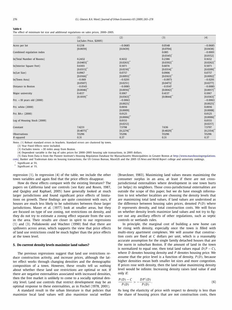
In Table 6, we turn to the correlation between lot size and salesprices. We use Banker and Tradesman data on housing price trans-actions between 2000 and 2005. Our basic regression is:

Log(SalesPrice) = α · LotSizeMinimum

+ HouseandTownCharacteristics. (5)

Our home characteristics include the year of construction, totalnumber of rooms, interior square footage and lot size. Our towncharacteristics include the year 2000 set of characteristics used inthe other regressions in Table 4.

Just as in the case of permits, there is a question of whetherland use restrictions will impact town-level prices or region-levelprices. In the case of permits, it is quite possible that local land userestrictions limit building in one town, but just more that buildingto another locale. In the case of prices, it is possible that land userestrictions have no impact on prices in one locale, relative to aclose substitute town, but still have an impact on area level prices.The basic economics of price restrictions tells us that we shouldnot expect the price of a good to rise relative to a perfect substituteif that goods supply is restricted. The question, then, is whetherhow close these small towns in Massachusetts are to being perfect

substitutes for one another. While we cannot answer this questionfully, we are confident that as we control for more area level char-acteristics, such as density and demographics, the towns are morelikely to be closer substitutes and we are less likely to find an ef-fect of land use restrictions on prices.

To see this, we present two types of regressions. First, we con-trol only for the relatively fixed attributes of the town: land area,distance to Boston, and the presence of a major university. We thenadd in controls for contemporaneous density, share of the popula-tion that is under 18 years old, share of the population that iswhite and share of the adult population with a college degree. Inthe first regression, the coefficient on acres per lot is 0.12, which ismarginally significant at 10%. This coefficient means that each ex-tra acre per lot is associated with a twelve percent increase in thevalue of a house. This supports the view that minimum lot sizerules do increase value for existing homeowners, and helps to ex-plain why homeowners find minimum lot sizes so appealing.

In the second regression, we include our control for contem-poraneous demographics and density, the coefficient flips sign andloses statistical significance. As such, there is certainly no impactof minimum lot size on prices once we make areas roughly com-parable. We interpret this finding as supporting the basic economicview that quantity limitations shouldn’t raise prices when housesare compared to very similar units.

In the third regression, also found in Table 6, we include bothacres per lot and the regulation index. In this case, both variableshave a positive effect on prices. The impact of the regulation in-dex on prices is statistically significant; the impact of minimumlot sizes is not. An interpretation of this finding is that differenttypes of land use regulations are positively correlated, but that thenon-lot size regulations are more effective at limiting the types ofdevelopment which would reduce prices, such as multi-unit sub-divisions that could change the demographic mix of the town. Thisfinding supports the view that it is important to measure a widerange of barriers beyond minimum lot size. However, it is worthemphasizing that the coefficient on acres per lot in regression (3)is not statistically distinct from the coefficient on acres per lot in



Table 6The effect of minimum lot size and additional regulations on sales prices, 2000–2005.

(1) (2) (3) (4)Ln(Sales Price, $2005)

Acres per lot 0.1218 −0.0685 0.0548 −0.0685[0.0659] [0.0439] [0.0704] [0.0438]

Combined regulation index 0.085 −0.0001[0.0345]* [0.0152]

ln(Total Number of Rooms) 0.2432 0.1632 0.2386 0.1632[0.0403]** [0.0263]** [0.0392]** [0.0262]**

ln(Interior Square Feet) 0.6103 0.5071 0.6074 0.5071[0.0313]** [0.0210]** [0.0314]** [0.0209]**

ln(Lot Size) 0.0967 0.0757 0.0906 0.0757[0.0166]** [0.0093]** [0.0163]** [0.0092]**

ln(Town Area) −0.069 −0.0291 −0.0973 −0.0291[0.0507] [0.0251] [0.0473]* [0.0277]

Distance to Boston −0.0143 −0.0085 −0.0147 −0.0085[0.0046]** [0.0016]** [0.0042]** [0.0017]**

Major university 0.4117 0.1067 0.4137 0.1067[0.1019]** [0.0363]** [0.0844]** [0.0363]**

Pct. <18 years old (2000) −0.0063 −0.0063[0.0025]* [0.0025]*

Pct. white (2000) 0.0016 0.0016[0.0009] [0.0008]

Pct. BA+ (2000) 0.0125 0.0125[0.0006]** [0.0006]**

Log of Housing Stock (2000) 0.0155 0.0155[0.0212] [0.0217]

Constant 7.4231 7.5798 7.636 7.5797[0.4075]** [0.2274]** [0.4029]** [0.2354]**

Observations 55296 55296 55296 55296R-squared 0.31 0.37 0.31 0.37

Notes. (1) Robust standard errors in brackets. Standard errors are clustered by town.(2) Year Fixed Effects were included.(3) Excludes towns >30 miles away from Boston.(4) Dependent variable is the log of sales prices for 2000–2005 housing sale transactions, in 2005 dollars.(5) Data from Data is from the Pioneer Institute’s Housing Regulation Database for Massachusetts Municipalities in Greater Boston at http://www.masshousingregulations.

com/, Banker and Tradesman data on housing transactions, the US Census Bureau, MassGIS and the 2005 US News and World Report college and university rankings.* Significant at 5%.


regression (1). In regression (4) of the table, we include the othertown variables and again find that the price effects disappear.

How do these effects compare with the existing literature? Thepapers on California land use controls (see Katz and Rosen, 1987,and Quigley and Raphael, 2005) have generally looked at muchlarger jurisdictions and found significant price effects of limita-tions on growth. These findings are quite consistent with ours, ifhouses are much less likely to be substitutes between those largerjurisdictions. Maser et al. (1977) look at smaller areas, but theyare focused on type of use zoning, not restrictions on density, andthey do not try to estimate a zoning effect separate from the usesin the area. Their results are closer in spirit to our regressions(1) and (3). Pollakowski and Wachter (1990) find that there arespillovers across areas, which supports the view that price effectsof land use restrictions could be much higher than the price effectsat the town level.

5. Do current density levels maximize land values?

The previous regressions suggest that land use restrictions re-duce construction activity, and increase prices, although the lat-ter effect works through changing densities and the demographiccomposition of a town. However, these results tell us nothingabout whether these land use restrictions are optimal or not. Ifthere are negative externalities associated with increased densities,then the free market is unlikely to come to a socially optimal den-sity level. Land use controls that restrict development may be anoptimal response to these externalities, as in Fischel (1978, 2001).

A standard result in the urban literature is that policies thatmaximize local land values will also maximize social welfare

(Brueckner, 1983). Maximizing land values means maximizing theconsumer surplus in an area, at least if there are not cross-jurisdictional externalities where development in one town hurts(or helps) its neighbors. Those cross-jurisdictional externalities areoutside the scope of this paper, but we do have enough informa-tion to test whether localities are choosing the density levels thatare maximizing total land values, if land values are understood asthe difference between housing sales prices, denoted P (D) whereD represents density, and total construction costs. We will focuson whether density levels maximize land values and not try to fig-ure out any ancillary effects of other regulations, such as septiccontrols or wetlands rules.

In principle, the marginal cost of building a new home canbe rising with density, especially once the town is filled withmulti-story apartment complexes. We will assume that construc-tion costs are fixed at C dollars per unit, which is a reasonablyaccurate assumption for the single family detached houses that arethe norm in suburban Boston. If the amount of land in the townis normalized to equal one, then total land values equal D(P − C),where D denotes housing density and P denotes housing price. Weassume that the price level is a function of density, P (D), becausehigher densities mean both smaller lot sizes and more congestion.If prices rose with density, then the land value maximizing densitylevel would be infinite. Increasing density raises land value if andonly if:

P (D) − C

P (D)> − D P ′(D)

P (D). (6)

As long the elasticity of price with respect to density is less thanthe share of housing prices that are not construction costs, then




Table 7Effect of density on sales prices, 2000–2005.

(1) (2) (3) (4) (5) (6)Ln(Sales Price, $2005)

Log of Housing Density (2000) −0.1246 −0.0042 −0.0994 0.019 −0.1609 −0.0518[0.0337]** [0.0165] [0.0399]* [0.0254] [0.0349]** [0.0611]

ln(Total Number of Rooms) 0.2451 0.1757 0.2532 0.1828 0.2423 0.2437[0.0431]** [0.0266]** [0.0431]** [0.0269]** [0.0431]** [0.0441]**

ln(Interior Square Feet) 0.6739 0.5565 0.6826 0.5582 0.6609 0.7016[0.0338]** [0.0197]** [0.0334]** [0.0199]** [0.0351]** [0.0401]**

Distance to Boston −0.0195 −0.0086 −0.0172 −0.0075 −0.0221 −0.014[0.0040]** [0.0016]** [0.0048]** [0.0017]** [0.0043]** [0.0058]*

Major university 0.3939 0.0967 0.3822 0.0957 0.4104 0.3635[0.0982]** [0.0384]* [0.0979]** [0.0375]* [0.0964]** [0.1039]**

Year 0.0871 0.0854 0.0867 0.085 0.0872 0.0868[0.0023]** [0.0023]** [0.0023]** [0.0023]** [0.0023]** [0.0023]**

Pct. <18 years old (2000) −0.0065 −0.0043[0.0025]** [0.0033]

Pct. white (2000) 0.0017 0.0024[0.0009] [0.0012]

Pct. BA+ (2000) 0.0126 0.0126[0.0006]** [0.0006]**

Constant −166.7604 −163.1347 −166.069 −162.4988 −166.796 −166.5293[4.6199]** [4.5109]** [4.6581]** [4.5347]** [4.6091]** [4.6478]**

IV for ln(Housing Density 2000) None None Avg. min. lot size Avg. min. lot size ln(Town Density in 1915) ln(Forest Cover in 1885)

Observations 56,204 56,204 55,299 55,299 56,204 55,448R-squared 0.31 0.37 0.3 0.37 0.3 0.3

Notes. (1) Robust standard errors in brackets. Standard errors are clustered by town.(2) Excludes towns >30 miles away from Boston.(3) Dependent variable is the log of sales prices for 2000–2005 housing sale transactions, in 2005 dollars.(4) Data is from the Pioneer Institute’s Housing Regulation Database for Massachusetts Municipalities in Greater Boston at http://www.masshousingregulations.com/,

Banker and Tradesman data on housing transactions, the US Census Bureau, the Harvard Forest Survey of Massachusetts, MassGIS and the 2005 US News and World Reportcollege and university rankings.

* Significant at 5%.** Significant at 1%.

more density increases local land values. The density level thatmaximizes total land values will cause Eq. (6) to hold with equal-ity.

To estimate, whether Eq. (6) holds for our sample of cities wemust both know the elasticity of housing prices with respect todensity and the share of housing prices that are not accountedfor by construction costs. We can estimate the value of P (D)−C

P (D)

for our sample using price and construction cost data. In 2004, inour sample, the average home cost $450,000 and had 1800 squarefeet of interior space. Using R.S. Means data on construction costs,Gyourko and Saiz (2004) estimate a 97 dollar per square foot costof new construction for the Boston area. These figures suggest thatthe physical structure in the average home costs 174,600 dollarsand that P (D)−C

P (D)equals 0.61. We cannot be confident about the

R.S. Means figure, but if construction costs were as high as 150dollars a square foot, then that ratio would still be equal to 0.4.

Table 7 provides our estimate of the total effect of area densityon housing prices. We do not control for unit lot size, since one ofthe effects of higher density is to reduce unit lot size, and theoryrequires us to include that effect in our estimate of the overallimpact of density on prices. We control for interior square feet,the number of rooms, distance to Boston and the presence of amajor university.9

The first regression shows the estimated ordinary least squaresestimate of −0.12. In the second regression, we include controlsfor share of the population that is less than 18, share of the adultpopulation with college degrees and share of the population thatis white. With these controls, the estimated coefficient is essen-tially zero. Controlling for contemporaneous demographics elim-

9 Since town areas are often larger for places with lower density levels, we ex-clude town area as a control. Our results are not sensitive to this exclusion.

inates the density effect, which suggests that density is primarilyimportant as a sorting device to change the composition of an area.

These results are potentially compromised since density levelsmay be driven by omitted housing characteristics that increase de-mand. Larger lot sizes may be the result of cheaper prices. Thisconcern means that standard hedonic regressions may understatethe true negative impact of density on housing prices. To addressthis concern, we use instruments for current density level usingthree instruments. Our first instrument is our own minimum lotsize variable. In regression (3), we repeat regression (1) using theminimum lot size variable as an instrument for housing density.The estimated density elasticity changes to −1. In regression (4),we repeat regression (2) and include other controls, but use mini-mum lot size as an instrument. In this case, the estimated elasticityis 0.02. Again, there is no effect of lot size once we control for thedemographics of the town.

In regressions (5) and (6), we use the log of town density in1915 and the forest cover of the town in 1885 as instruments. Wedo not include other controls, but if we did they would again leadto coefficients of close to zero. When we use 1915 density as an in-strument, we estimate a coefficient of −0.16. When we use forestcover, we estimate a coefficient of −0.05. Our range of estimateddensity elasticities, therefore, lies between 0.02 and −0.16.

Even if we believe that controlling for demographics is inappro-priate because those variables themselves reflect density levels, thedensity coefficients are much lower than the estimated land shareof housing costs. Localities seem to have density levels that are toolow to currently maximize land values. To us, this is the primarypuzzle produced by this paper: why aren’t communities choosingdensity levels to maximize their land values?

One possible explanation of this fact is that densities are basedon historical conditions that don’t reflect current demand. A sec-ond explanation is that zoning decisions are made without the



possibility of transfers between builders and current owners.10

The absence of these transfers, which are essentially illegal inMassachusetts, makes it difficult for existing homeowners to reapmany benefits from new development.

These results do not imply that the current situation is subopti-mal. There may be externalities associated with new developmentthat have impacts outside of the local area and these may meanthat it is desirable to restrict new construction below the level thatwould maximize land values. A fuller accounting of all the globalexternalities from new building would be necessary to make anyclear welfare claims, and that is beyond the scope of this paper.

6. Conclusion

Over the last 25 years, Greater Boston has seen a remarkable in-crease in housing prices and a decline in the number of new units.This change reflects increasingly restricted supply. The reductionin supply doesn’t reflect an exogenous lack of land. There has beenno significant increase in density levels associated with decliningconstruction.

Development is greater in dense places. Lot sizes are increas-ing, not falling. The value of land when it extends an existing lotis not great. Instead, the decline in new construction and asso-ciated increase in price reflects increasing man-made barriers tonew construction.

In this paper, we catalog the barriers to new construction. Mini-mum lot size is the most important of these measures, but increas-ingly new barriers have been added, like wetlands and septic rules.These barriers have all increased over time, but there is little clearpattern about where they have been adopted beyond. Recreationalwater increases water-related barriers. Current minimum lot sizesmainly reflect historical density patterns.

The impact of lot size on new development is quite clear. Eachextra acre per lot is associated with about 40 percent fewer per-mits between 1980 and 2002. The impact of other controls onconstruction is weaker, but it does appear in a specification withtown fixed effects that each extra rule reduces new constructionby about 10 percent. Minimum lot size and other regulations areassociated with higher prices, but as urban theory predicts, thiseffect disappears when we control for a wide range of area levelvariables.

Regulations do appear to increase prices, but the impact of den-sity on prices is generally quite modest. As a result, communities

10 Fischel (1978) is the classic analysis of the property rights issues surroundingland use controls.

seem to have density levels that are far too low to be maximiz-ing their land values. This suggests the possibility that currentland use controls are suboptimally restrictive, and it leaves us withthe puzzle of understanding why communities are not choosing tomaximize land values.

References

Brueckner, J.K., 1983. Property value maximization and public-sector efficiency. Jour-nal of Urban Economics 14, 1–15.

Brueckner, J.K., 1990. Growth controls and land values in an open city. Land Eco-nomics 66, 237–248.

Dain, A., 2006. Reference Guide to Residential Land-Use Regulation in EasternMassachusetts: A Study of 187 Communities. Rappaport Institute for GreaterBoston, Harvard University/Pioneer Institute for Public Policy Research, Cam-bridge/Boston.

Ellickson, R.C., 1977. Suburban growth controls: An economic and legal analysis. YaleLaw Journal 86 (3), 385–511.

Evenson, B., Wheaton, W.C., 2003. Local variation in land use regulation. Brookings-Wharton Papers on Urban Affairs, 221–260.

Fischel, W.A., 1978. A property rights approach to municipal zoning. Land Eco-nomics 54 (1), 64–81.

Fischel, W.A., 2001. The Homevoter Hypothesis. Harvard University Press, Cam-bridge, MA.

Glaeser, E., Gyourko, J., 2003. The impact of building restrictions on housing af-fordability. Federal Reserve Bank of New York Economic Policy Review 9 (2),21–39.

Glaeser, E., Gyourko, J., Saks, R., 2005. Why have housing prices gone up? AmericanEconomic Review Papers and Proceedings 95 (2), 329–333.

Glaeser, E.L., Kahn, M., Rappaport, J., 2008. Why do the poor live in cities? The roleof public transportation. Journal of Urban Economics 63 (1), 1–24.

Gyourko, J., Saiz, A., 2004. Reinvestment in the housing stock: The role of construc-tion costs and the supply side. Journal of Urban Economics 55 (2), 238–256.

Gyourko, J., Saiz, A., 2006. Construction costs and the supply of housing structure.Journal of Regional Science 46 (4), 661–680.

Ihlanfeldt, K., 2007. The effect of land use regulation on housing and land prices.Journal of Urban Economics 61, 420–435.

Jakabovics, A., 2006. Housing affordability initiative: Land use research findings.http://web.mit.edu/cre/research/hai/land-use.html.

Katz, L., Rosen, K.T., 1987. The interjursdictional effects of growth controls on hous-ing prices. Journal of Law and Economics 30 (1), 149–160.

Levine, N., 1999. The effects of local growth controls on regional housing produc-tion and population redistribution in California. Urban Studies 36 (12), 2047–2068.

Maser, S., Riker, W., Rosett, R., 1977. The effects of zoning and externalities on theprice of land: An empirical analysis of Monroe County, New York. Journal of Lawand Economics 20 (1), 111–132.

Pollakowski, H.O., Wachter, S.M., 1990. The effects of land-use constraints on hous-ing prices. Land Economics 66 (3), 315–324.

Quigley, J.M., Raphael, S., 2005. Regulation and the high cost of housing in Califor-nia. American Economic Review 95 (2), 323–329.

http://web.mit.edu/cre/research/hai/land-use.html

the causes and consequences of land use regulation...

Documents