the bugs project examples volume 1
TRANSCRIPT

Examples Volume 1
Rats: Normal hierarchical model
Pump: conjugate gamma-Poisson hierarchical model
Dogs: log linear binary model
Seeds: random effects logistic regression
Surgical: institutional ranking
Salm: extra-Poisson variation in dose-response study
Equiv: bioequivalence in a cross-over trial
Dyes: variance components model
Stacks: robust and ridge regression
Epil: repeated measures on Poisson counts
Blocker: random effects meta-analysis of clinical trials
Oxford: smooth fit to log-odds ratios in case control studies
LSAT: latent variable models for item-response data
Bones: latent trait model for multiple ordered catagorical responses
Inhalers: random effects model for ordinal responses from a cross-over trial
Mice: Weibull regression in censored survival analysis
Kidney: Weibull regression with random effects
Leuk: survival analysis using Cox regression
Cox regression with frailties
References:Sorry - an on-line version of the references is currently unavailable.
Contents
[1]

Please refer to the existing Examples documentation available fromhttp://www.mrc-bsu.cam.ac.uk/bugs.
Contents
[2]

Rats: a normal hierarchical model
This example is taken from section 6 of Gelfand et al (1990), and concerns 30 young rats whoseweights were measured weekly for five weeks. Part of the data is shown below, where Yij is theweight of the ith rat measured at age xj.
A plot of the 30 growth curves suggests some evidence of downward curvature.
The model is essentially a random effects linear growth curve
Yij ~ Normal(αi + β i(xj - xbar), τc)
αi ~ Normal(αc, τα)
β i ~ Normal(βc, τβ)
where xbar = 22, and τ represents the precision (1/variance) of a normal distribution. We note theabsence of a parameter representing correlation between α i and β i unlike in Gelfand et al 1990.However, see the Birats example in Volume 2 which does explicitly model the covariancebetween αi and β i. For now, we standardise the xj's around their mean to reduce dependencebetween αi and β i in their likelihood: in fact for the full balanced data, complete independence isachieved. (Note that, in general, prior independence does not force the posterior distributions tobe independent).
αc , τα , βc , τβ , τc are given independent ``noninformative'' priors. Interest particularly focuseson the intercept at zero time (birth), denoted α0 = αc - βc xbar.
Graphical model for rats example:
Weights Yij of rat i on day xjxj = 8 15 22 29 36
__________________________________Rat 1 151 199 246 283 320Rat 2 145 199 249 293 354.......Rat 30 153 200 244 286 324
Rats Examples Volume I
[3]

BUGS language for rats example:
model{
for( i in 1 : N ) {for( j in 1 : T ) {
Y[i , j] ~ dnorm(mu[i , j],tau.c)mu[i , j] <- alpha[i] + beta[i] * (x[j] - xbar)
}alpha[i] ~ dnorm(alpha.c,alpha.tau)beta[i] ~ dnorm(beta.c,beta.tau)
}tau.c ~ dgamma(0.001,0.001)sigma <- 1 / sqrt(tau.c)alpha.c ~ dnorm(0.0,1.0E-6)alpha.tau ~ dgamma(0.001,0.001)beta.c ~ dnorm(0.0,1.0E-6)beta.tau ~ dgamma(0.001,0.001)alpha0 <- alpha.c - xbar * beta.c
}
Note the use of a very flat but conjugate prior for the population effects: a locally uniform prior
for(j IN 1 : T)
for(i IN 1 : N)
sigma
tau.c
x[j]
Y[i, j]
mu[i, j]
beta[i]alpha[i]
beta.taubeta.calpha0alpha.calpha.tau
Examples Volume I Rats
[4]

could also have been used.
Data ( click to open )
Inits ( click to open )
(Note: the response data (Y) for the rats example can also be found in the file ratsy.odc inrectangular format. The covariate data (X) can be found in S-Plus format in file ratsx.odc. To loaddata from each of these files, focus the window containing the open data file before clicking on"load data" from the "Specification" dialog.)
Results
A 1000 update burn in followed by a further 10000 updates gave the parameter estimates:
These results may be compared with Figure 5 of Gelfand et al 1990 --- we note that the meangradient of independent fitted straight lines is 6.19.
Gelfand et al 1990 also consider the problem of missing data, and delete the last observation ofcases 6-10, the last two from 11-20, the last 3 from 21-25 and the last 4 from 26-30. Theappropriate data file is obtained by simply replacing data values by NA (see below). The modelspecification is unchanged, since the distinction between observed and unobserved quantities ismade in the data file and not the model specification.
Data ( click to open )
Gelfand et al 1990 focus on the parameter estimates and the predictions for the final 4observations on rat 26. These predictions are obtained automatically in BUGS by monitoring therelevant Y[] nodes. The following estimates were obtained:
We note that our estimate 6.58 of βc is substantially greater than that shown in Figure 6 ofGelfand et al 1990. However, plotting the growth curves indicates some curvature with steepergradients at the beginning: the mean of the estimated gradients of the reduced data is 6.66,compared to 6.19 for the full data. Hence we are inclined to believe our analysis. The observed
mean sd MC_error val2.5pc median val97.5pc start samplealpha0 106.6 3.655 0.04079 99.44 106.5 113.8 1001 10000beta.c 6.185 0.1061 0.00132 5.975 6.185 6.394 1001 10000sigma 6.086 0.4606 0.007398 5.255 6.061 7.049 1001 10000
mean sd MC_error val2.5pc median val97.5pc start sampleY[26,2] 204.6 8.689 0.1145 187.6 204.7 221.4 1001 10000Y[26,3] 250.2 10.21 0.1732 230.1 250.2 270.5 1001 10000Y[26,4] 295.6 12.5 0.228 270.6 295.5 319.7 1001 10000Y[26,5] 341.2 15.29 0.2936 310.7 341.3 370.9 1001 10000beta.c 6.578 0.1497 0.003415 6.284 6.578 6.87 1001 10000
Rats Examples Volume I
[5]

weights for rat 26 were 207, 257, 303 and 345, compared to our predictions of 204, 250, 295and 341.
Examples Volume I Rats
[6]

Dogs: loglinear model for binary data
Lindley (19??) analyses data from Kalbfleisch (1985) on the Solomon-Wynne experiment ondogs, whereby they learn to avoid an electric shock. A dog is put in a compartment, the lights areturned out and a barrier is raised, and 10 seconds later an electric shock is applied. The resultsare recorded as success (Y = 1 ) if the dog jumps the barrier before the shock occurs, or failure(Y = 0) otherwise.
Thirty dogs were each subjected to 25 such trials. A plausible model is to suppose that a doglearns from previous trials, with the probability of success depending on the number of previousshocks and the number of previous avoidances. Lindley thus uses the following model
π j = Axj Bj-xj
for the probability of a shock (failure) at trial j, where xj = number of success (avoidances) beforetrial j and j - xj = number of previous failures (shocks). This is equivalent to the following log linearmodel
log π j = αxj + β ( j-xj )
Hence we have a generalised linear model for binary data, but with a log-link function rather thanthe canonical logit link. This is trivial to implement in BUGS:
model{
for (i in 1 : Dogs) {xa[i, 1] <- 0; xs[i, 1] <- 0 p[i, 1] <- 0for (j in 2 : Trials) {
xa[i, j] <- sum(Y[i, 1 : j - 1])xs[i, j] <- j - 1 - xa[i, j]log(p[i, j]) <- alpha * xa[i, j] + beta * xs[i, j]y[i, j] <- 1 - Y[i, j]y[i, j] ~ dbern(p[i, j])
}}alpha ~ dnorm(0, 0.00001)I(, -0.00001)beta ~ dnorm(0, 0.00001)I(, -0.00001)A <- exp(alpha)B <- exp(beta)
}
Dogs Examples Volume I
[7]
Data ( click to open )
Inits( click to open )
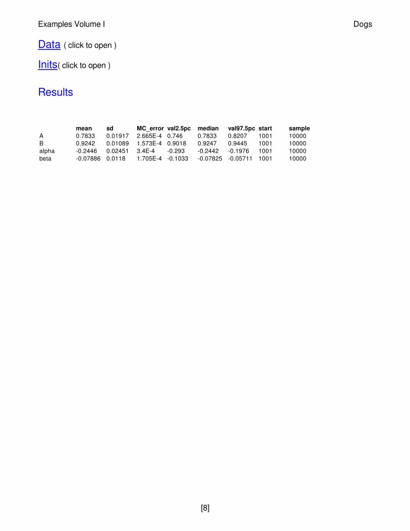
Results
mean sd MC_error val2.5pc median val97.5pc start sampleA 0.7833 0.01917 2.665E-4 0.746 0.7833 0.8207 1001 10000B 0.9242 0.01089 1.573E-4 0.9018 0.9247 0.9445 1001 10000alpha -0.2446 0.02451 3.4E-4 -0.293 -0.2442 -0.1976 1001 10000beta -0.07886 0.0118 1.705E-4 -0.1033 -0.07825 -0.05711 1001 10000
Examples Volume I Dogs
[8]
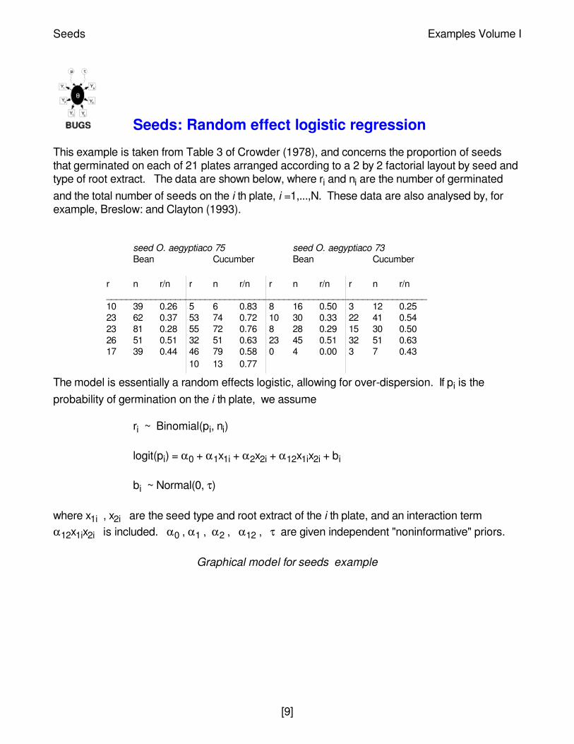
Seeds: Random effect logistic regression
This example is taken from Table 3 of Crowder (1978), and concerns the proportion of seedsthat germinated on each of 21 plates arranged according to a 2 by 2 factorial layout by seed andtype of root extract. The data are shown below, where ri and ni are the number of germinatedand the total number of seeds on the i th plate, i =1,...,N. These data are also analysed by, forexample, Breslow: and Clayton (1993).
The model is essentially a random effects logistic, allowing for over-dispersion. If pi is theprobability of germination on the i th plate, we assume
ri ~ Binomial(pi, ni)
logit(pi) = α0 + α1x1i + α2x2i + α12x1ix2i + bi
bi ~ Normal(0, τ)
where x1i , x2i are the seed type and root extract of the i th plate, and an interaction termα12x1ix2i is included. α0 , α1 , α2 , α12 , τ are given independent "noninformative" priors.
Graphical model for seeds example
seed O. aegyptiaco 75 seed O. aegyptiaco 73Bean Cucumber Bean Cucumber
r n r/n r n r/n r n r/n r n r/n_________________________________________________________________10 39 0.26 5 6 0.83 8 16 0.50 3 12 0.2523 62 0.37 53 74 0.72 10 30 0.33 22 41 0.5423 81 0.28 55 72 0.76 8 28 0.29 15 30 0.5026 51 0.51 32 51 0.63 23 45 0.51 32 51 0.6317 39 0.44 46 79 0.58 0 4 0.00 3 7 0.43
10 13 0.77
Seeds Examples Volume I
[9]
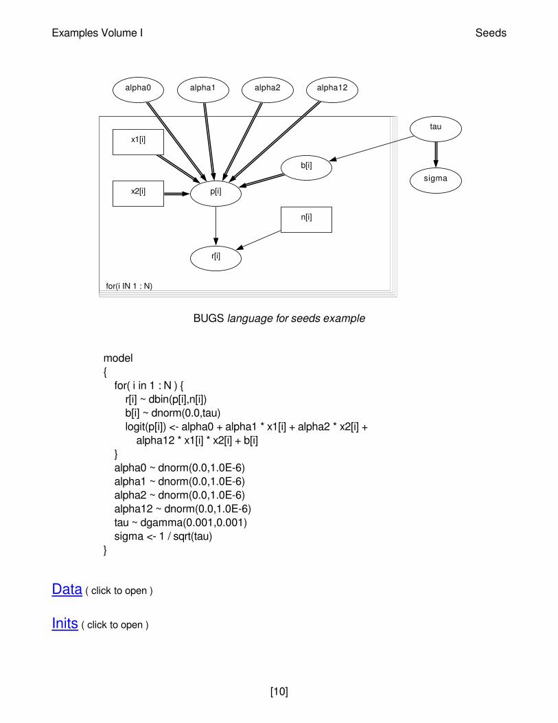
BUGS language for seeds example
model{
for( i in 1 : N ) {r[i] ~ dbin(p[i],n[i])b[i] ~ dnorm(0.0,tau)logit(p[i]) <- alpha0 + alpha1 * x1[i] + alpha2 * x2[i] +
alpha12 * x1[i] * x2[i] + b[i]}alpha0 ~ dnorm(0.0,1.0E-6)alpha1 ~ dnorm(0.0,1.0E-6)alpha2 ~ dnorm(0.0,1.0E-6)alpha12 ~ dnorm(0.0,1.0E-6)tau ~ dgamma(0.001,0.001)sigma <- 1 / sqrt(tau)
}
Data ( click to open )
Inits ( click to open )
for(i IN 1 : N)
sigma
tau
alpha12alpha2alpha1alpha0
b[i]
n[i]
x1[i]
x2[i] p[i]
r[i]
Examples Volume I Seeds
[10]
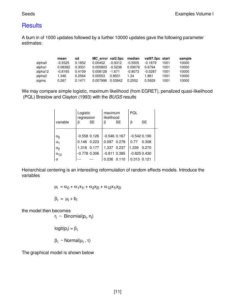
Results
A burn in of 1000 updates followed by a further 10000 updates gave the following parameterestimates:
We may compare simple logistic, maximum likelihood (from EGRET), penalized quasi-likelihood(PQL) Breslow and Clayton (1993) with the BUGS results
Heirarchical centering is an interesting reformulation of random effects models. Introduce thevariables
µi = α0 + α1x1i + α2x2i + α12x1ix2i
β i = µi + bi
the model then becomesri ~ Binomial(pi, ni)
logit(pi) = β i
β i ~ Normal(µi , τ)
The graphical model is shown below
mean sd MC_error val2.5pc median val97.5pc start samplealpha0 -0.5525 0.1852 0.00402 -0.9312 -0.5505 -0.1879 1001 10000alpha1 0.08382 0.3031 0.005803 -0.5238 0.09076 0.6794 1001 10000alpha12 -0.8165 0.4109 0.008128 -1.671 -0.8073 -0.0287 1001 10000alpha2 1.346 0.2564 0.00553 0.8501 1.34 1.881 1001 10000sigma 0.267 0.1471 0.007996 0.03842 0.2552 0.5929 1001 10000
Logistic maximum PQLregression likelihood
variable β SE β SE β SE_________________________________________________
α0 -0.558 0.126 -0.546 0.167 -0.542 0.190α1 0.146 0.223 0.097 0.278 0.77 0.308α2 1.318 0.177 1.337 0.237 1.339 0.270α12 -0.778 0.306 -0.811 0.385 -0.825 0.430σ --- --- 0.236 0.110 0.313 0.121
Seeds Examples Volume I
[11]

This formulation of the model has two advantages: the squence of random numbers generatedby the Gibbs sampler has better correlation properties and the time per update is reducedbecause the updating for the α parameters is now conjugate.
for(i IN 1 : N)
beta[i]
p[i]
sigma
tau
alpha12alpha2alpha1alpha0
n[i]
x1[i]
x2[i]
mu[i]
r[i]
Examples Volume I Seeds
[12]

Surgical: Institutional ranking
This example considers mortality rates in 12 hospitals performing cardiac surgery in babies. Thedata are shown below.
The number of deaths ri for hospital i are modelled as a binary response variable with `true'failure probability pi:
ri ~ Binomial(pi, ni)
We first assume that the true failure probabilities are independent (i.e.fixed effects) for eachhospital. This is equivalent to assuming a standard non-informative prior distribution for the pi's,namely:
pi ~ Beta(1.0, 1.0)
Graphical model for fixed effects surgical example:
Hospital No of ops No of deaths__________________________________A 47 0B 148 18C 119 8D 810 46E 211 8F 196 13G 148 9H 215 31I 207 14J 97 8K 256 29L 360 24
Surgical Examples Volume I
[13]

BUGS language for fixed effects surgical model:
model{
for( i in 1 : N ) {p[i] ~ dbeta(1.0, 1.0)
r[i] ~ dbin(p[i], n[i])}
}
Data ( click to open )
Inits ( click to open )
A more realistic model for the surgical data is to assume that the failure rates across hospitalsare similar in some way. This is equivalent to specifying a random effects model for the truefailure probabilities pi as follows:
logit(pi) = bi
bi ~ Normal(µ, τ)
Standard non-informative priors are then specified for the population mean (logit) probability offailure, µ, and precision, τ.
Graphical model for random effects surgical example:
for(i IN 1 : N)
n[i]p[i]
r[i]
Examples Volume I Surgical
[14]
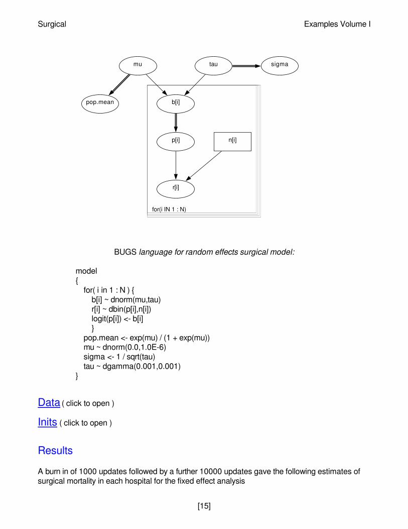
BUGS language for random effects surgical model:
model{
for( i in 1 : N ) {b[i] ~ dnorm(mu,tau)r[i] ~ dbin(p[i],n[i])logit(p[i]) <- b[i]}
pop.mean <- exp(mu) / (1 + exp(mu))mu ~ dnorm(0.0,1.0E-6)sigma <- 1 / sqrt(tau)tau ~ dgamma(0.001,0.001)
}
Data ( click to open )
Inits ( click to open )
Results
A burn in of 1000 updates followed by a further 10000 updates gave the following estimates ofsurgical mortality in each hospital for the fixed effect analysis
for(i IN 1 : N)
sigma
pop.mean
taumu
b[i]
n[i]p[i]
r[i]
Surgical Examples Volume I
[15]

and for the random effects analysis
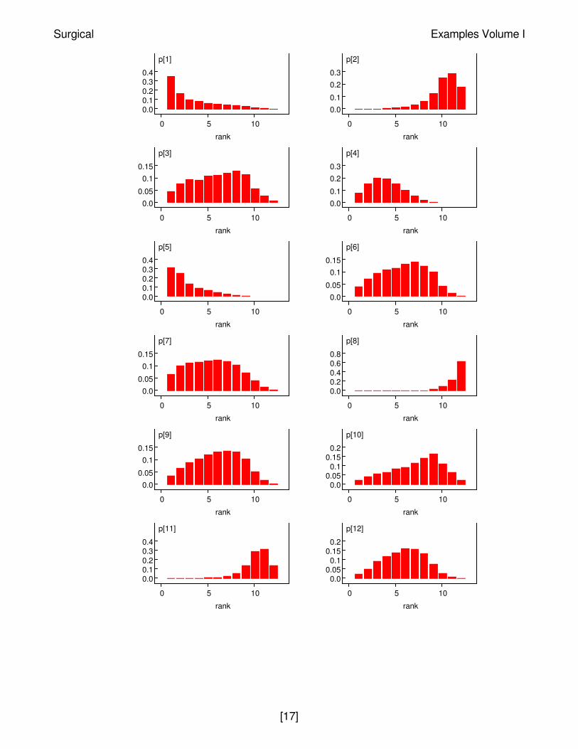
A particular strength of the Markov chain Monte Carlo (Gibbs sampling) approach implementedin BUGS is the ability to make inferences on arbitrary functions of unknown model parameters.For example, we may compute the rank probabilty of failure for each hospital at each iteration.This yields a sample from the posterior distribution of the ranks.
The figures below show the posterior ranks for the estimated surgical mortality rate in eachhospital for the random effect models. These are obtained by setting the rank monitor for variablep (select the "Rank" option from the "Statistics" menu) after the burn-in phase, and then selectingthe "histogram" option from this menu after a further 10000 updates. These distributions illustratethe considerable uncertainty associated with 'league tables': there are only 2 hospitals (H and K)whose intervals exclude the median rank and none whose intervals fall completely within thelower or upper quartiles.
Plots of distribution of ranks of true failure probability for random effects model:
mean sd MC_error val2.5pc median val97.5pc start samplep[1] 0.02009 0.01946 2.085E-4 6.091E-4 0.01441 0.07178 1001 10000p[2] 0.1266 0.0271 2.67E-4 0.07853 0.125 0.1845 1001 10000p[3] 0.07436 0.02371 2.349E-4 0.03492 0.07181 0.1265 1001 10000p[4] 0.05789 0.00824 8.136E-5 0.04264 0.05762 0.07487 1001 10000p[5] 0.04237 0.01388 1.096E-4 0.01972 0.04086 0.07362 1001 10000p[6] 0.07081 0.01811 1.935E-4 0.0397 0.06931 0.1098 1001 10000p[7] 0.06686 0.02025 1.872E-4 0.03259 0.06493 0.111 1001 10000p[8] 0.1473 0.02393 2.681E-4 0.1039 0.146 0.1983 1001 10000p[9] 0.07216 0.0179 1.59E-4 0.04093 0.07071 0.1104 1001 10000p[10] 0.09078 0.0288 3.122E-4 0.04274 0.08817 0.1531 1001 10000p[11] 0.1165 0.02009 2.074E-4 0.08 0.1155 0.1589 1001 10000p[12] 0.06906 0.01345 1.261E-4 0.04518 0.06816 0.0977 1001 10000
mean sd MC_error val2.5pc median val97.5pc start samplemu -2.558 0.1554 0.002585 -2.884 -2.551 -2.266 1001 10000p[1] 0.05302 0.01948 3.565E-4 0.01802 0.05221 0.09348 1001 10000p[2] 0.1029 0.02196 2.976E-4 0.06712 0.1006 0.152 1001 10000p[3] 0.07044 0.01727 1.978E-4 0.0397 0.06916 0.1079 1001 10000p[4] 0.0593 0.007985 1.212E-4 0.04458 0.05897 0.07591 1001 10000p[5] 0.05187 0.01329 2.269E-4 0.02791 0.05102 0.07961 1001 10000p[6] 0.06903 0.01448 1.564E-4 0.04284 0.06854 0.1004 1001 10000p[7] 0.06682 0.01602 1.773E-4 0.03835 0.06595 0.1009 1001 10000p[8] 0.1226 0.02244 4.014E-4 0.08196 0.1217 0.1698 1001 10000p[9] 0.0698 0.01432 1.508E-4 0.04432 0.06901 0.1004 1001 10000p[10] 0.07851 0.01955 2.03E-4 0.04506 0.07662 0.1217 1001 10000p[11] 0.1021 0.01761 2.283E-4 0.07158 0.1009 0.1398 1001 10000p[12] 0.06858 0.01168 1.301E-4 0.04745 0.06805 0.09349 1001 10000pop.mean 0.07259 0.01028 1.696E-4 0.05293 0.07235 0.09401 1001 10000sigma 0.4028 0.16 0.003672 0.1577 0.3793 0.7872 1001 10000
Examples Volume I Surgical
[16]
p[1]
rank
0 5 10
0.0 0.1 0.2 0.3 0.4
p[2]
rank
0 5 10
0.0 0.1
0.2 0.3
p[3]
rank
0 5 10
0.0 0.05
0.1 0.15
p[4]
rank
0 5 10
0.0 0.1
0.2 0.3
p[5]
rank
0 5 10
0.0 0.1 0.2 0.3 0.4
p[6]
rank
0 5 10
0.0 0.05
0.1 0.15
p[7]
rank
0 5 10
0.0 0.05
0.1 0.15
p[8]
rank
0 5 10
0.0 0.2 0.4 0.6 0.8
p[9]
rank
0 5 10
0.0 0.05
0.1 0.15
p[10]
rank
0 5 10
0.0 0.05 0.1 0.15 0.2
p[11]
rank
0 5 10
0.0 0.1 0.2 0.3 0.4
p[12]
rank
0 5 10
0.0 0.05 0.1 0.15 0.2
Surgical Examples Volume I
[17]

Salm: extra - Poisson variation in dose - responsestudy
Breslow (1984) analyses some mutagenicity assay data (shown below) on salmonella in whichthree plates have been processed at each dose i of quinoline and the number of revertantcolonies of TA98 Salmonella measured. A certain dose-response curve is suggested by theory.
This is assumed to be a random effects Poisson model allowing for over-dispersion. Let xi bethe dose on the plates i1, i2 and i3. Then we assume
yij ~ Poisson(µij)
log(µij) = α + β log(xi + 10) + γxi + λij
λij ~ Normal(0, τ)
α , β , γ , τ are given independent ``noninformative'' priors. The appropriate graph is shown
Graphical model for salm example
dose of quinoline (µg per plate)
0 10 33 100 333 1000_______________________________15 16 16 27 33 2021 18 26 41 38 2729 21 33 69 41 42
Examples Volume I Salm
[18]
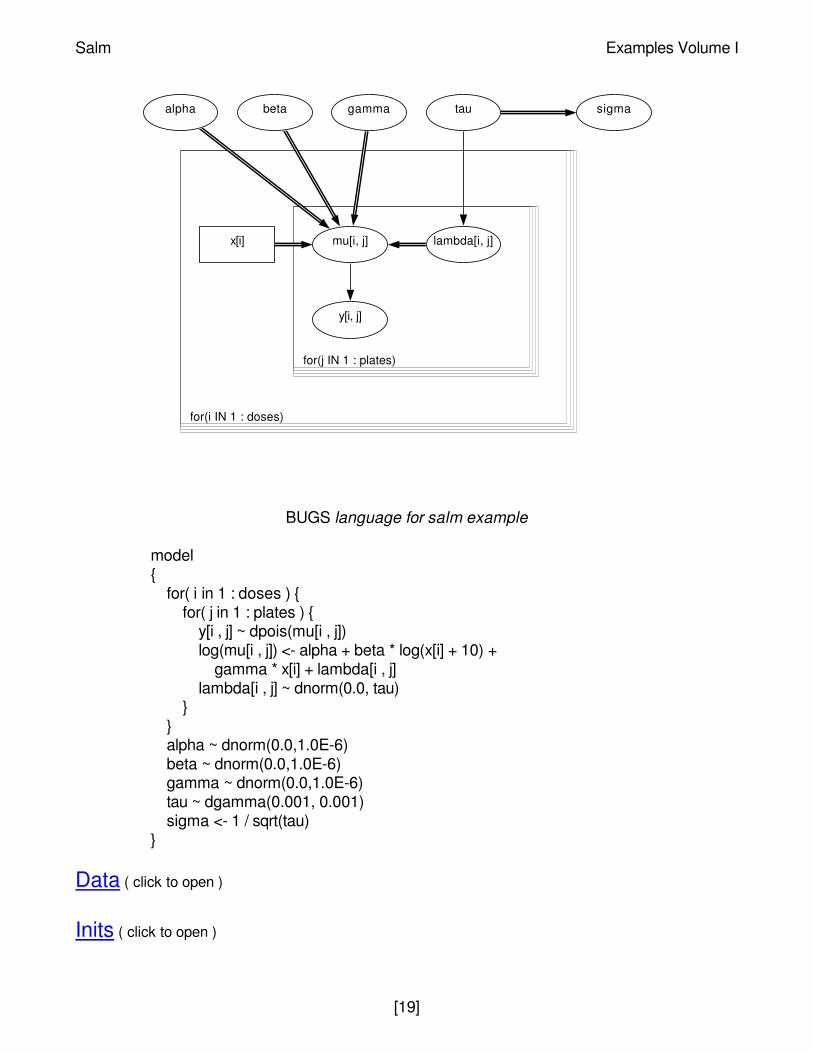
BUGS language for salm example
model{
for( i in 1 : doses ) {for( j in 1 : plates ) {
y[i , j] ~ dpois(mu[i , j])log(mu[i , j]) <- alpha + beta * log(x[i] + 10) +
gamma * x[i] + lambda[i , j]lambda[i , j] ~ dnorm(0.0, tau)
}}alpha ~ dnorm(0.0,1.0E-6)beta ~ dnorm(0.0,1.0E-6)gamma ~ dnorm(0.0,1.0E-6)tau ~ dgamma(0.001, 0.001)sigma <- 1 / sqrt(tau)
}
Data ( click to open )
Inits ( click to open )
for(i IN 1 : doses)
for(j IN 1 : plates)
sigmataugammabetaalpha
x[i] lambda[i, j]mu[i, j]
y[i, j]
Salm Examples Volume I
[19]

Results
A 1000 update burn in followed by a further 10000 updates gave the parameter estimates
These estimates can be compared with the quasi-likelihood estimates of Breslow (1984) whoreported α = 2.203 +/- 0.363, β = 0.311 +/- 0.099, γ = -9.74E-4 +/- 4.37E-4, σ = 0.268
mean sd MC_error val2.5pc median val97.5pc start samplealpha 2.193 0.3874 0.01118 1.438 2.194 2.959 1001 10000beta 0.3059 0.1054 0.003266 0.09692 0.3065 0.5131 1001 10000gamma -9.577E-4 4.525E-4 1.48E-5 -0.001837 -9.622E-4 -3.196E-5 1001 10000sigma 0.2608 0.08077 0.002114 0.1305 0.2512 0.4472 1001 10000
Examples Volume I Salm
[20]
Equiv: bioequivalence in a cross-over trial
The table below shows some data from a two-treatment, two-period crossover trial to compare 2tablets A and B, as reported by Gelfand et al (1990).
The response Yik from the i th subject (i = 1,...,10) in the k th period (k = 1,2) is assumed to be ofthe form
Yik ~ Normal(mik, τ1)
mik = µ + (-1)Tik - 1 φ / 2 + (-1)k - 1 π / 2 + δ i
δ i ~ Normal(0, τ2)
where Tik= 1,2 denotes the treatment given to subject i in period k, µ, φ, π are the overall mean,treatment and period effects respectively, and δ i represents the random effect for subject i. Thegraph of this model and its BUGS language description are shown below
Graphical model for equiv example
Subject i Sequence seq Period 1 Ti1 Period 2 Ti2________________________________________________________________________1 AB 1 1.40 1 1.65 22 AB 1 1.64 1 1.57 23 BA -1 1.44 2 1.58 1....8 AB 1 1.25 1 1.44 29 BA -1 1.25 2 1.39 110 BA -1 1.30 2 1.52 1
Equiv Examples Volume I
[21]
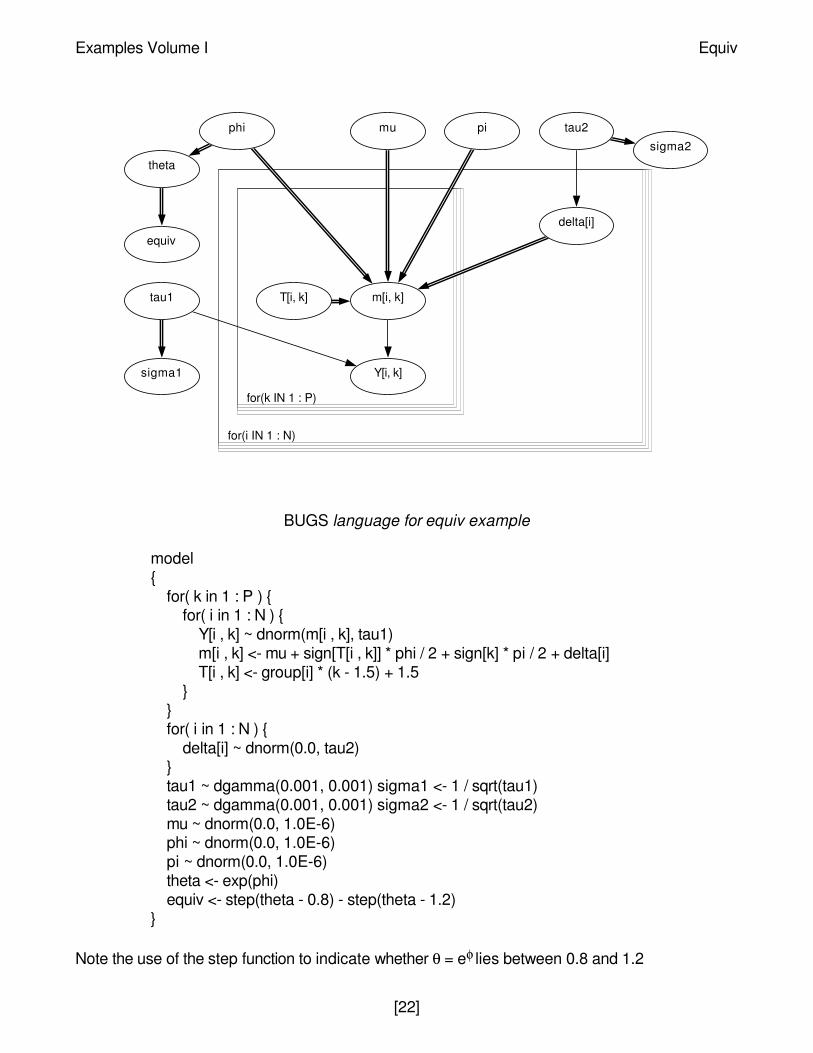
BUGS language for equiv example
model{
for( k in 1 : P ) {for( i in 1 : N ) {
Y[i , k] ~ dnorm(m[i , k], tau1)m[i , k] <- mu + sign[T[i , k]] * phi / 2 + sign[k] * pi / 2 + delta[i]T[i , k] <- group[i] * (k - 1.5) + 1.5
}}for( i in 1 : N ) {
delta[i] ~ dnorm(0.0, tau2)}tau1 ~ dgamma(0.001, 0.001) sigma1 <- 1 / sqrt(tau1)tau2 ~ dgamma(0.001, 0.001) sigma2 <- 1 / sqrt(tau2)mu ~ dnorm(0.0, 1.0E-6)phi ~ dnorm(0.0, 1.0E-6)pi ~ dnorm(0.0, 1.0E-6)theta <- exp(phi)equiv <- step(theta - 0.8) - step(theta - 1.2)
}
Note the use of the step function to indicate whether θ = eφ lies between 0.8 and 1.2
for(i IN 1 : N)
for(k IN 1 : P)
sigma2
sigma1
equiv
theta
muphi pi tau2
tau1
delta[i]
T[i, k] m[i, k]
Y[i, k]
Examples Volume I Equiv
[22]

which traditionally determines bioequivelence.
Data ( click to open )
Inits ( click to open )
Results
A 1000 update burn in followed by a further 10000 updates gave the parameteresestimates
mean sd MC_error val2.5pc median val97.5pc start sampleequiv 0.9976 0.04893 5.148E-4 1.0 1.0 1.0 1001 10000mu 1.437 0.05364 0.001822 1.329 1.437 1.542 1001 10000phi -0.008338 0.05201 5.151E-4 -0.1127 -0.008502 0.09926 1001 10000pi -0.1802 0.05189 4.793E-4 -0.2834 -0.1803 -0.07353 1001 10000sigma1 0.1106 0.03374 9.345E-4 0.06492 0.1033 0.194 1001 10000sigma2 0.1399 0.05357 0.001464 0.04614 0.1355 0.2624 1001 10000theta 0.993 0.05181 5.125E-4 0.8934 0.9915 1.104 1001 10000
Equiv Examples Volume I
[23]

Dyes: variance components model
Box and Tiao (1973) analyse data first presented by Davies (1967) concerning batch to batchvariation in yields of dyestuff. The data (shown below) arise from a balanced experiment wherebythe total product yield was determined for 5 samples from each of 6 randomly chosen batches ofraw material.
The object of the study was to determine the relative importance of between batch variationversus variation due to sampling and analytic errors. On the assumption that the batches andsamples vary independently, and contribute additively to the total error variance, we may assumethe following model for dyestuff yield:
yij ~ Normal(µi, τwithin)
µi ~ Normal(θ, τbetween)
where yij is the yield for sample j of batch i, µi is the true yield for batch i, τwithin is the inverse ofthe within-batch variance σ2within ( i.e. the variation due to sampling and analytic error), θ is thetrue average yield for all batches and τbetween is the inverse of the between-batch variances2between. The total variation in product yield is thus σ2total = σ2within + σ2between and the relativecontributions of each component to the total variance are fwithin = σ2within / σ2total and fbetween =
σ2between / σ2total . We assume standard non-informative priors for θ, τwithin and τbetween.
Graphical model for dyes example
Batch Yield (in grams)_______________________________________1 1545 1440 1440 1520 15802 1540 1555 1490 1560 14953 1595 1550 1605 1510 15604 1445 1440 1595 1465 15455 1595 1630 1515 1635 16256 1520 1455 1450 1480 1445
Examples Volume I Dyes
[24]
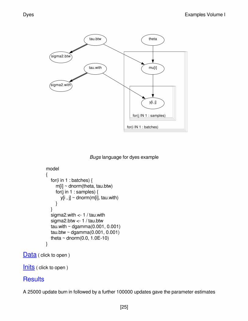
Bugs language for dyes example
model{
for(i in 1 : batches) {m[i] ~ dnorm(theta, tau.btw)for(j in 1 : samples) {
y[i , j] ~ dnorm(m[i], tau.with)}
}sigma2.with <- 1 / tau.withsigma2.btw <- 1 / tau.btwtau.with ~ dgamma(0.001, 0.001)tau.btw ~ dgamma(0.001, 0.001)theta ~ dnorm(0.0, 1.0E-10)
}
Data ( click to open )
Inits ( click to open )
Results
A 25000 update burn in followed by a further 100000 updates gave the parameter estimates
for(j IN 1 : samples)
for(i IN 1 : batches)
sigma2.btw
sigma2.with
tau.btw
tau.with
theta
mu[i]
y[i, j]
Dyes Examples Volume I
[25]

Note that a relatively long run was required because of the high autocorrelation betweensuccessively sampled values of some parameters. Such correlations reduce the 'effective' sizeof the posterior sample, and hence a longer run is needed to ensure sufficient precision of theposterior estimates. Note that the posterior distribution for σ2between has a very long upper tail:
hence the posterior mean is considerably larger than the median. Box and Tiao estimate σ2within
= 2451 and σ2between = 1764 by classical analysis of variance. Here, σ2between is estimated bythe difference of the between- and within-batch mean squares divided by the number of batches -1. In cases where the between-batch mean square within-batch mean square, this leads to theunsatisfactory situation of a negative variance estimate. Computing a confidence interval forσ2between is also difficult using the classical approach due to its complicated samplingdistribution
mean sd MC_error val2.5pc median val97.5pc start samplesigma2.btw 2207.0 4289.0 40.94 0.008042 1290.0 10210.0 25001 100000sigma2.with 3034.0 1102.0 19.89 1561.0 2807.0 5752.0 25001 100000theta 1528.0 21.5 0.1712 1484.0 1527.0 1571.0 25001 100000
Examples Volume I Dyes
[26]

Stacks: robust regression
Birkes and Dodge (1993) apply different regression models to the much-analysed stack-lossdata of Brownlee (1965). This features 21 daily responses of stack loss y, the amount ofammonia escaping, with covariates being air flow x1, temperature x2 and acid concentrationx3. Part of the data is shown below.
We first assume a linear regression on the expectation of y, with a variety of different errorstructures. Specifically
µi = β0 + β1z1i + β2z2i + β3z3i
yi ~ Normal(µi, τ)
yi ~ Double exp(µi, τ)
yi ~ t(µi, τ, d)
where zij = (xij - xbarj) /sd(xj) are covariates standardised to have zero mean and unit variance.β1, β2, β3 are initially given independent "noninformative" priors.
Maximum likelihood estimates for the double expontential (Laplace) distribution are essentiallyequivalent to minimising the sum of absolute deviations (LAD), while the other options arealternative heavy-tailed distributions. A t on 4 degrees of freedom has been chosen, althoughwith more data it would be possible to allow this parameter also to be unknown.
We also consider the use of 'ridge regression', intended to avoid the instability due to correlatedcovariates. This has been shown Lindley and Smith (1972) to be equivalent to assuming theregression coefficients of the standardised covariates to be exchangeable, so that
β j ~ Normal(0, φ), j = 1, 2, 3.
In the following example we extend the work of Birkes and Dodge (1993) by applying this ridge
Day Stack loss y air flow x1 temperature x2 acid x3_______________________________________________________________1 42 80 27 892 37 80 27 88.....21 15 70 20 91
Stacks Examples Volume I
[27]

technique to each of the possible error distributions.
Birkes and Dodge (1993) suggest investigating outliers by examining residuals yi - µi greaterthan 2.5 standard deviations. We can calculate standardised residuals for each of thesedistributions, and create a variable outlier[i] taking on the value 1 whenever this condition isfulfilled. Mean values of outlier[i] then show the confidence with which this definition of outlier isfulfilled.
The BUGS language for all the models is shown below, with all models except the normal linearregression commented out:
model{# Standardise x's and coefficients
for (j in 1 : p) {b[j] <- beta[j] / sd(x[ , j ])for (i in 1 : N) {
z[i, j] <- (x[i, j] - mean(x[, j])) / sd(x[ , j])}
}b0 <- beta0 - b[1] * mean(x[, 1]) - b[2] * mean(x[, 2]) - b[3] * mean(x[, 3])
# Modeld <- 4; # degrees of freedom for t
for (i in 1 : N) {Y[i] ~ dnorm(mu[i], tau)
# Y[i] ~ ddexp(mu[i], tau)# Y[i] ~ dt(mu[i], tau, d)
mu[i] <- beta0 + beta[1] * z[i, 1] + beta[2] * z[i, 2] + beta[3] * z[i, 3]stres[i] <- (Y[i] - mu[i]) / sigmaoutlier[i] <- step(stres[i] - 2.5) + step(-(stres[i] + 2.5) )
}# Priors
beta0 ~ dnorm(0, 0.00001)for (j in 1 : p) {
beta[j] ~ dnorm(0, 0.00001) # coeffs independent# beta[j] ~ dnorm(0, phi) # coeffs exchangeable (ridge regression)
}tau ~ dgamma(1.0E-3, 1.0E-3)phi ~ dgamma(1.0E-2,1.0E-2)
# standard deviation of error distributionsigma <- sqrt(1 / tau) # normal errors
# sigma <- sqrt(2) / tau # double exponential errors# sigma <- sqrt(d / (tau * (d - 2))); # t errors on d degrees of freedom}
Examples Volume I Stacks
[28]
Data ( click to open )
Inits ( click to open )
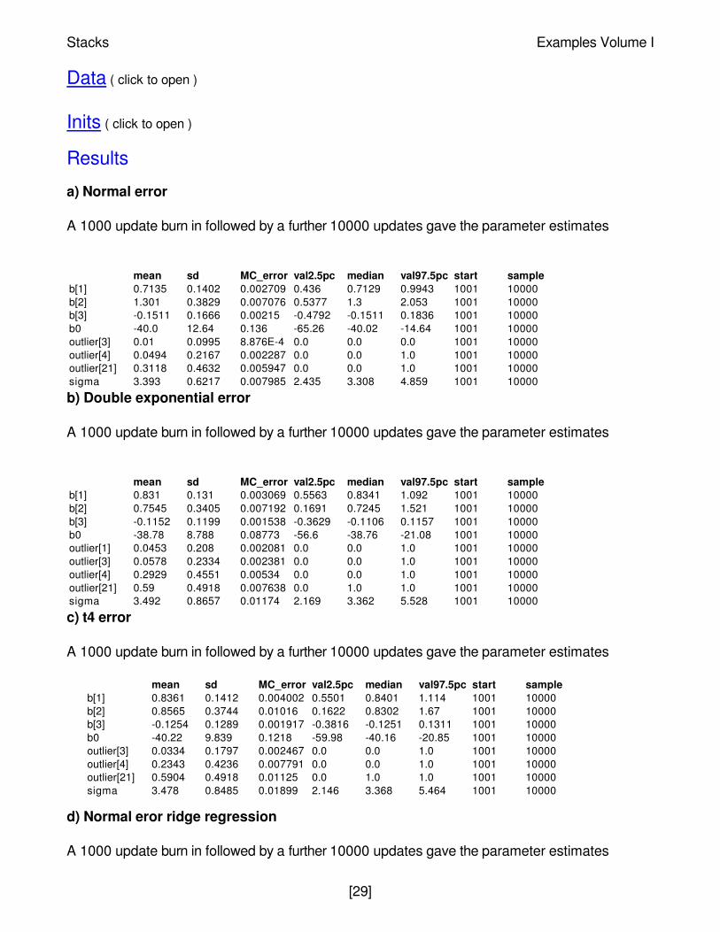
Results
a) Normal error
A 1000 update burn in followed by a further 10000 updates gave the parameter estimates
b) Double exponential error
A 1000 update burn in followed by a further 10000 updates gave the parameter estimates
c) t4 error
A 1000 update burn in followed by a further 10000 updates gave the parameter estimates
d) Normal eror ridge regression
A 1000 update burn in followed by a further 10000 updates gave the parameter estimates
mean sd MC_error val2.5pc median val97.5pc start sampleb[1] 0.7135 0.1402 0.002709 0.436 0.7129 0.9943 1001 10000b[2] 1.301 0.3829 0.007076 0.5377 1.3 2.053 1001 10000b[3] -0.1511 0.1666 0.00215 -0.4792 -0.1511 0.1836 1001 10000b0 -40.0 12.64 0.136 -65.26 -40.02 -14.64 1001 10000outlier[3] 0.01 0.0995 8.876E-4 0.0 0.0 0.0 1001 10000outlier[4] 0.0494 0.2167 0.002287 0.0 0.0 1.0 1001 10000outlier[21] 0.3118 0.4632 0.005947 0.0 0.0 1.0 1001 10000sigma 3.393 0.6217 0.007985 2.435 3.308 4.859 1001 10000
mean sd MC_error val2.5pc median val97.5pc start sampleb[1] 0.831 0.131 0.003069 0.5563 0.8341 1.092 1001 10000b[2] 0.7545 0.3405 0.007192 0.1691 0.7245 1.521 1001 10000b[3] -0.1152 0.1199 0.001538 -0.3629 -0.1106 0.1157 1001 10000b0 -38.78 8.788 0.08773 -56.6 -38.76 -21.08 1001 10000outlier[1] 0.0453 0.208 0.002081 0.0 0.0 1.0 1001 10000outlier[3] 0.0578 0.2334 0.002381 0.0 0.0 1.0 1001 10000outlier[4] 0.2929 0.4551 0.00534 0.0 0.0 1.0 1001 10000outlier[21] 0.59 0.4918 0.007638 0.0 1.0 1.0 1001 10000sigma 3.492 0.8657 0.01174 2.169 3.362 5.528 1001 10000
mean sd MC_error val2.5pc median val97.5pc start sampleb[1] 0.8361 0.1412 0.004002 0.5501 0.8401 1.114 1001 10000b[2] 0.8565 0.3744 0.01016 0.1622 0.8302 1.67 1001 10000b[3] -0.1254 0.1289 0.001917 -0.3816 -0.1251 0.1311 1001 10000b0 -40.22 9.839 0.1218 -59.98 -40.16 -20.85 1001 10000outlier[3] 0.0334 0.1797 0.002467 0.0 0.0 1.0 1001 10000outlier[4] 0.2343 0.4236 0.007791 0.0 0.0 1.0 1001 10000outlier[21] 0.5904 0.4918 0.01125 0.0 1.0 1.0 1001 10000sigma 3.478 0.8485 0.01899 2.146 3.368 5.464 1001 10000
Stacks Examples Volume I
[29]
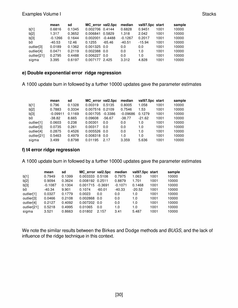
e) Double exponential error ridge regression
A 1000 update burn in followed by a further 10000 updates gave the parameter estimates
f) t4 error ridge regression
A 1000 update burn in followed by a further 10000 updates gave the parameter estimates
We note the similar results between the Birkes and Dodge methods and BUGS, and the lack ofinfluence of the ridge technique in this context.
mean sd MC_error val2.5pc median val97.5pc start sampleb[1] 0.6816 0.1345 0.002706 0.4144 0.6828 0.9451 1001 10000b[2] 1.317 0.3652 0.006841 0.5829 1.318 2.042 1001 10000b[3] -0.1266 0.1644 0.002001 -0.4488 -0.1267 0.2017 1001 10000b0 -40.53 12.46 0.1255 -65.46 -40.51 -15.94 1001 10000outlier[3] 0.0189 0.1362 0.001325 0.0 0.0 0.0 1001 10000outlier[4] 0.0471 0.2119 0.002388 0.0 0.0 1.0 1001 10000outlier[21] 0.2795 0.4488 0.006227 0.0 0.0 1.0 1001 10000sigma 3.395 0.6197 0.007177 2.425 3.312 4.828 1001 10000
mean sd MC_error val2.5pc median val97.5pc start sampleb[1] 0.796 0.1328 0.00319 0.5135 0.8005 1.058 1001 10000b[2] 0.7883 0.3334 0.007516 0.2109 0.7546 1.53 1001 10000b[3] -0.09911 0.1169 0.001705 -0.3386 -0.09686 0.1279 1001 10000b0 -38.82 8.665 0.09608 -56.67 -38.77 -21.62 1001 10000outlier[1] 0.0603 0.238 0.00301 0.0 0.0 1.0 1001 10000outlier[3] 0.0735 0.261 0.00317 0.0 0.0 1.0 1001 10000outlier[4] 0.2875 0.4526 0.005526 0.0 0.0 1.0 1001 10000outlier[21] 0.5463 0.4979 0.008318 0.0 1.0 1.0 1001 10000sigma 3.499 0.8798 0.01195 2.17 3.359 5.636 1001 10000
mean sd MC_error val2.5pc median val97.5pc start sampleb[1] 0.7949 0.1399 0.003333 0.5108 0.7975 1.063 1001 10000b[2] 0.9094 0.3624 0.008192 0.2511 0.8879 1.701 1001 10000b[3] -0.1087 0.1304 0.001715 -0.3691 -0.1071 0.1468 1001 10000b0 -40.34 9.901 0.1074 -60.01 -40.33 -20.52 1001 10000outlier[1] 0.0327 0.1779 0.0023 0.0 0.0 1.0 1001 10000outlier[3] 0.0466 0.2108 0.002868 0.0 0.0 1.0 1001 10000outlier[4] 0.2127 0.4092 0.007202 0.0 0.0 1.0 1001 10000outlier[21] 0.5218 0.4995 0.01065 0.0 1.0 1.0 1001 10000sigma 3.521 0.8663 0.01802 2.157 3.41 5.487 1001 10000
Examples Volume I Stacks
[30]
Blocker: random effects meta-analysis of clinicaltrials
Carlin (1992) considers a Bayesian approach to meta-analysis, and includes the followingexamples of 22 trials of beta-blockers to prevent mortality after myocardial infarction.
In a random effects meta-analysis we assume the true effect (on a log-odds scale) δ i in a trial i isdrawn from some population distribution.Let rCi denote number of events in the control group intrial i, and rTi denote events under active treatment in trial i. Our model is:
rCi ~ Binomial(pCi, nCi)
rTi ~ Binomial(pTi, nTi)
logit(pCi) = µi
logit(pTi) = µi + δ i
δ i ~ Normal(d, τ)
``Noninformative'' priors are given for the µi's. τ and d. The graph for this model is shown inbelow. We want to make inferences about the population effect d, and the predictive distributionfor the effect δnew in a new trial. Empirical Bayes methods estimate d and τ by maximumlikelihood and use these estimates to form the predictive distribution p(δnew | dhat, τhat ). FullBayes allows for the uncertainty concerning d and τ.
Graphical model for blocker example:
Study Mortality: deaths / totalTreated Control
_____________________________________________1 3/38 3/392 7/114 14/1163 5/69 11/934 102/1533 127/1520.....20 32/209 40/21821 27/391 43/36422 22/680 39/674
Blockers Examples Volume I
[31]
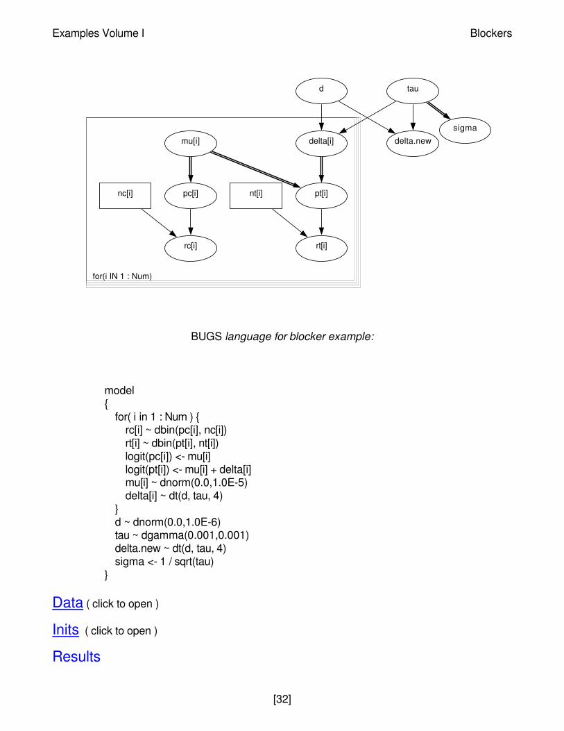
BUGS language for blocker example:
model{
for( i in 1 : Num ) {rc[i] ~ dbin(pc[i], nc[i])rt[i] ~ dbin(pt[i], nt[i])logit(pc[i]) <- mu[i]logit(pt[i]) <- mu[i] + delta[i]mu[i] ~ dnorm(0.0,1.0E-5)delta[i] ~ dt(d, tau, 4)
}d ~ dnorm(0.0,1.0E-6)tau ~ dgamma(0.001,0.001)delta.new ~ dt(d, tau, 4)sigma <- 1 / sqrt(tau)
}
Data ( click to open )
Inits ( click to open )
Results
for(i IN 1 : Num)
sigma
taud
delta.newmu[i] delta[i]
pt[i]nt[i]pc[i]nc[i]
rt[i]rc[i]
Examples Volume I Blockers
[32]

A 1000 update burn in followed by a further 10000 updates gave the parameter estimates
Our estimates are lower and with tighter precision - in fact similar to the values obtained byCarlin for the empirical Bayes estimator. The discrepancy appears to be due to Carlin's use of auniform prior for σ2 in his analysis, which will lead to increased posterior mean and standard
deviation for d, as compared to our (approximate) use of p(σ2) ~ 1 / σ2 (see his Figure 1).
In some circumstances it might be reasonable to assume that the population distribution hasheavier tails, for example a t distribution with low degrees of freedom. This is easilyaccomplished in BUGS by using the dt distribution function instead of dnorm for δ and δnew.
mean sd MC_error val2.5pc median val97.5pc start sampled -0.2492 0.06422 0.002004 -0.3727 -0.2502 -0.1194 1001 10000delta.new -0.2499 0.1509 0.002389 -0.5592 -0.2536 0.07169 1001 10000sigma 0.1189 0.07 0.003521 0.02428 0.1067 0.2825 1001 10000
Blockers Examples Volume I
[33]
Oxford: smooth fit to log-odds ratios
Breslow and Clayton (1993) re-analyse 2 by 2 tables of cases (deaths from childhood cancer)and controls tabulated against maternal exposure to X-rays, one table for each of 120combinations of age (0-9) and birth year (1944-1964). The data may be arranged to the followingform.
Their most complex model is equivalent to expressing the log(odds-ratio) ψi for the table instratum i as
logψ i = α + β1yeari + β2(yeari2 - 22) + bi
bi ~ Normal(0, τ)
They use a quasi-likelihood approximation of the full hypergeometric likelihood obtained byconditioning on the margins of the tables.
We let r0i denote number of exposures among the n0i controls in stratum i, and r1i denote
number of exposures for the n1i cases. The we assume
r0i ~ Binomial(p0i, n0
i)
r1i ~ Binomial(p1i, n1i)
logit(p0i) = µi
logit(p1i) = µi + logψ i
Assuming this model with independent vague priors for the µi's provides the correct conditionallikelihood. The appropriate graph is shown below
Strata Exposure: X-ray / totalCases Controls age year - 1954
_______________________________________________________________1 3/28 0/28 9 -10.....120 7/32 1/32 1 10
Examples Volume I Oxford
[34]
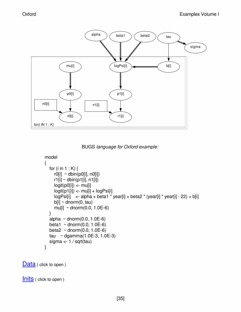
BUGS language for Oxford example:
model{
for (i in 1 : K) {r0[i] ~ dbin(p0[i], n0[i])r1[i] ~ dbin(p1[i], n1[i])logit(p0[i]) <- mu[i]logit(p1[i]) <- mu[i] + logPsi[i]logPsi[i] <- alpha + beta1 * year[i] + beta2 * (year[i] * year[i] - 22) + b[i]b[i] ~ dnorm(0, tau)mu[i] ~ dnorm(0.0, 1.0E-6)
}alpha ~ dnorm(0.0, 1.0E-6)beta1 ~ dnorm(0.0, 1.0E-6)beta2 ~ dnorm(0.0, 1.0E-6)tau ~ dgamma(1.0E-3, 1.0E-3)sigma <- 1 / sqrt(tau)
}
Data ( click to open )
Inits ( click to open )
for(i IN 1 : K)
sigma
taubeta2beta1alpha
b[i]
n1[i]n0[i]
r1[i]
p1[i]
logPsi[i]mu[i]
p0[i]
r0[i]
Oxford Examples Volume I
[35]

Results
A 1000 update burn in followed by a further 10000 updates gave the parameter estimates
These estimates compare well with Breslow and Clayton (1993) PQL estimates of α = 0.566 +/-0.070, β1 = -0.469 +/- 0.0167, β2 = 0.0071 +/- 0.0033, σ = 0.15 +/- 0.10.
mean sd MC_error val2.5pc median val97.5pc start samplealpha 0.579 0.062 0.001545 0.4587 0.5793 0.7037 1001 10000beta1 -0.04557 0.01553 3.929E-4 -0.07688 -0.0457 -0.01586 1001 10000beta2 0.007041 0.003084 8.953E-5 0.001018 0.007004 0.01314 1001 10000sigma 0.09697 0.06011 0.005036 0.02419 0.08059 0.2457 1001 10000
Examples Volume I Oxford
[36]
LSAT: item response
Section 6 of the Law School Aptitude Test (LSAT) is a 5-item multiple choice test; studentsscore 1 on each item for the correct answer and 0 otherwise, giving R = 32 possible responsepatterns.Boch and Lieberman (1970) present data on LSAT for N = 1000 students, part of whichis shown below.
The above data may be analysed using the one-parameter Rasch model (see Andersen (1980),pp.253-254; Boch and Aitkin (1981)). The probability pjk that student j responds correctly to itemk is assumed to follow a logistic function parameterized by an `item difficulty' or thresholdparameter αk and a latent variable θj representing the student's underlying ability. The abilityparameters are assumed to have a Normal distribution in the population of students. That is:
logit(pjk) = θj - αk, j = 1,...,1000; k = 1,...,5
θj ~ Normal(0, τ)
The above model is equivalent to the following random effects logistic regression:
logit(pjk) = βθj - αk, j = 1,...,1000; k = 1,...,5
θj ~ Normal(0, 1)
where β corresponds to the scale parameter (β2 = τ) of the latent ability distribution. We assumea half-normal distribution with small precision for β; this represents vague prior information butconstrains β to be positive. Standard vague normal priors are assumed for the αk's. Note thatthe location of the αk's depend upon the mean of the prior distribution for θj which we have
Pattern index Item response pattern Freq (m)________________________________________________
1 0 0 0 0 0 32 0 0 0 0 1 63 0 0 0 1 0 2. . . . . . .. . . . . . .. . . . . . .30 1 1 1 0 1 6131 1 1 1 1 0 2832 1 1 1 1 1 298
LSAT Examples Volume I
[37]
arbitrarily fixed to be zero. Alternatively, Boch and Aitkin ensure identifiability by imposing a sum-to-zero constraint on the αk's. Hence we calculate ak = αk - αbar to enable comparision of theBUGS posterior parameter estimates with the Boch and Aitkin marginal maximum likelihoodestimates.
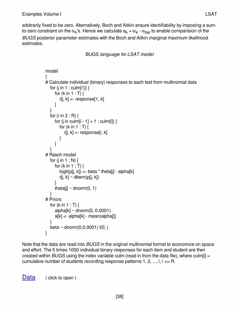
BUGS language for LSAT model
model{# Calculate individual (binary) responses to each test from multinomial data
for (j in 1 : culm[1]) {for (k in 1 : T) {
r[j, k] <- response[1, k]}
}for (i in 2 : R) {
for (j in culm[i - 1] + 1 : culm[i]) {for (k in 1 : T) {
r[j, k] <- response[i, k]}
}}
# Rasch modelfor (j in 1 : N) {
for (k in 1 : T) {logit(p[j, k]) <- beta * theta[j] - alpha[k]r[j, k] ~ dbern(p[j, k])
}theta[j] ~ dnorm(0, 1)
}# Priors
for (k in 1 : T) {alpha[k] ~ dnorm(0, 0.0001)a[k] <- alpha[k] - mean(alpha[])
}beta ~ dnorm(0,0.0001) I(0, )
}
Note that the data are read into BUGS in the original multinomial format to economize on spaceand effort. The 5 times 1000 individual binary responses for each item and student are thencreated within BUGS using the index variable culm (read in from the data file), where culm[i] =cumulative number of students recording response patterns 1, 2, ..., i; i <= R.
Data ( click to open )
Examples Volume I LSAT
[38]
Inits ( click to open )
Results
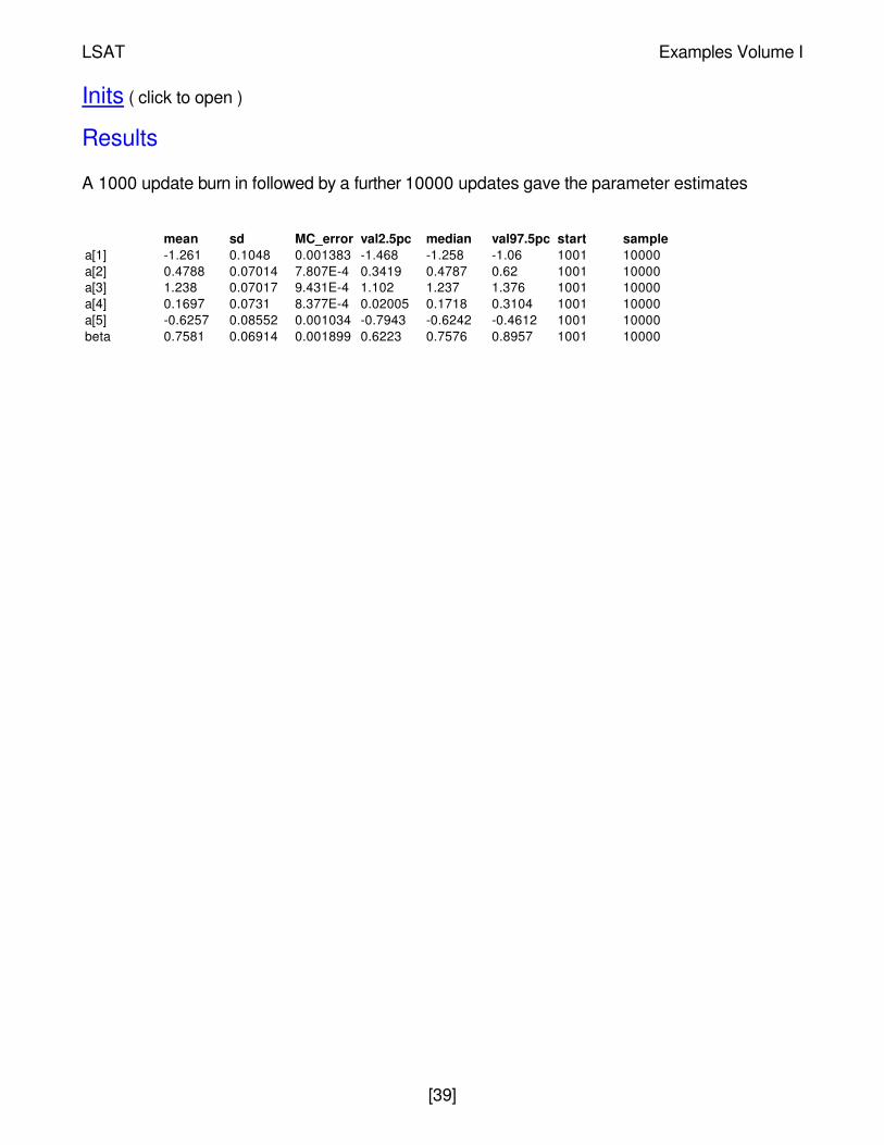
A 1000 update burn in followed by a further 10000 updates gave the parameter estimates
mean sd MC_error val2.5pc median val97.5pc start samplea[1] -1.261 0.1048 0.001383 -1.468 -1.258 -1.06 1001 10000a[2] 0.4788 0.07014 7.807E-4 0.3419 0.4787 0.62 1001 10000a[3] 1.238 0.07017 9.431E-4 1.102 1.237 1.376 1001 10000a[4] 0.1697 0.0731 8.377E-4 0.02005 0.1718 0.3104 1001 10000a[5] -0.6257 0.08552 0.001034 -0.7943 -0.6242 -0.4612 1001 10000beta 0.7581 0.06914 0.001899 0.6223 0.7576 0.8957 1001 10000
LSAT Examples Volume I
[39]

Bones: latent trait model for multipleordered catagorical responses
The concept of skeletal age (SA) arises from the idea that individuals mature at different rates:for any given chronological age (CA), the average SA in a sample of individuals should equaltheir CA, but with an inter-individual spread which reflects the differential rate of maturation.Roche et al (1975) have developed a model for predicting SA by calibrating 34 indicators(items) of skeletal maturity which may be observed in a radiograph. Each indicator iscategorized with respect to its degree of maturity: 19 are binary items (i.e. 0 = immature or 1 =mature); 8 items have 3 grades (i.e. 0 = immature; 1 = partially mature; 2 = fully mature); 1 itemhas 4 ordered grades and the remaining 6 items have 5 ordered grades of maturity. Roche et al.calculated threshold parameters for the boundarys between grades for each indicator. For thebinary items, there is a single threshold representing the CA at which 50% of individuals aremature for the indicator. Three-category items have 2 threshold parameters: the first correspondsto the CA at which 50% of individuals are either partially or fully mature for the indicator; thesecond is the CA at which 50% of individuals are fully mature. Four and five-category items have3 and 4 threshold parameters respectively, which are interpreted in a similar manner to those for3-category items. In addition, Roche et al. calculated a discriminability (slope) parameter foreach item which reflects its rate of maturation. Part of this data is shown below. Columns 1--4represent the threshold parameters (note the use of the missing value code NA to `fill in' thecolumns for items with fewer than 4 thresholds); column 5 is the discriminability parameter;column 6 gives the number of grades per item.
Thissen (1986) (p.71) presents the following graded radiograph data on 13 boys whose
Threshold parameters Discriminability Num grades_____________________________________________________________0.7425 NA NA NA 2.9541 210.2670 NA NA NA 0.6603 210.5215 NA NA NA 0.7965 29.3877 NA NA NA 1.0495 20.2593 NA NA NA 5.7874 2. . . . . .. . . . . .0.3887 1.0153 NA NA 8.1123 33.2573 7.0421 NA NA 0.9974 3. . . . . .. . . . . .15.4750 16.9406 17.4944 NA 1.4297 4. . . . . .. . . . . .5.0022 6.3704 8.2832 10.4988 1.0954 54.0168 5.1537 7.1053 10.3038 1.5329 5
Examples Volume I Bones
[40]

chronological ages range from 6 months to 18 years. (Note that for ease of implementation inBUGS we have listed the items in a different order to that used by Thissen):
Some items have missing data (represented by the code NA in the table above). This does notpresent a problem for BUGS: the missing grades are simply treated as unknown parameters tobe estimated along with the other parameters of interest such as the SA for each boy.
Thissen models the above data using the logistic function. For each item j and each grade k, thecumulative probability Qjk that a boy with skeletal age θ is assigned a more mature grade than kis given by
logitQjk = δ j(θ - γjk)
where δ j is the discriminability parameter and the γjk are the threshold parameters for item j.Hence the probability of observing an immature grade (i.e. k =1) for a particular skeletal age θ ispj,1 = 1 - Qj,1. The probability of observing a fully mature grade (i.e.k = Kj, where Kj is the numberof grades for item j is pj,Kj = Qj,Kj -1. For items with 3 or more categories, the probability of
observing an itermediate grade is pj,k = Qj,k-1 - Qj,k (i.e. the difference between the cumulativeprobability of being assigned grade k or more, and of being assigned grade k+1 or more).
The BUGS language for this model is given below. Note that the θi for each boy i is assigned avague, independent normal prior theta[i] ~ dnorm(0.0, 0.001). That is, each boy is treated as aseparate problem with is no `learning' or `borrowing strength' across individuals, and hence nohierachical structure on the θi's.
BUGS language for bones example
model{
for (i in 1 : nChild) {theta[i] ~ dnorm(0.0, 0.001)for (j in 1 : nInd) {
# Cumulative probability of > grade k given thetafor (k in 1: ncat[j] - 1) {
logit(Q[i, j, k]) <- delta[j] * (theta[i] - gamma[j, k])
ID CA Maturity grades for items 1 - 32___________________________________________________________________1 0.6 1 1 1 1 1 1 1 1 1 1 1 1 1 1 1 1 1 1 1 2 1 1 1 1 1 1 1 1 2 1 1 2 1 12 1.0 2 1 1 1 2 2 1 1 1 1 1 1 1 1 1 1 1 1 1 3 1 1 1 1 1 1 1 1 3 1 1 2 1 1. . . . . . . . . . . . . . . . . . . . . . . . . . . . . . . . . . . . . . . . . . . . . . . . .. . . . . . . . . . . . . . . . . . . . . . . . . . . . . . . . . . . . . . . . . . . . . . . . .12 16.0 2 2 2 2 2 2 2 2 2 2 2 2 2 2 2 2 2 2 2 3 3 3 1 NA 2 1 3 2 5 5 5 5 5 513 18.0 2 2 2 2 2 2 2 2 2 2 NA 2 2 2 2 2 2 2 2 3 3 3 NA 2 NA 2 3 4 5 5 5 5 5 5
Bones Examples Volume I
[41]

}}
# Probability of observing grade k given thetafor (j in 1 : nInd) {
p[i, j, 1] <- 1 - Q[i, j, 1]for (k in 2 : ncat[j] - 1) {
p[i, j, k] <- Q[i, j, k - 1] - Q[i, j, k]}p[i, j, ncat[j]] <- Q[i, j, ncat[j] - 1]grade[i, j] ~ dcat(p[i, j, 1 : ncat[j]])
}}
}
Data ( click to open )
Inits ( click to open )
We note a couple of tricks used in the above code. Firstly, the variable p has been declared as a3-way rectangular array with the size of the third dimension equal to the maximum number ofpossible grades (i.e.5) for all items (even though items 1--28 have fewer than 5 categories). Thestatement
grade[i, j] ~ dcat(p[i, j, 1 :ngrade[j]])
is then used to select the relevant elements of p[i,j, ] for item j, thus ignoring any `empty' spacesin the array for items with fewer than the maximum number of grades. Secondly, the final sectionof the above code includes a loop indexed as follows
Results
A 1000 update burn in followed by a further 10000 updates gave the parameter estimates
Examples Volume I Bones
[42]
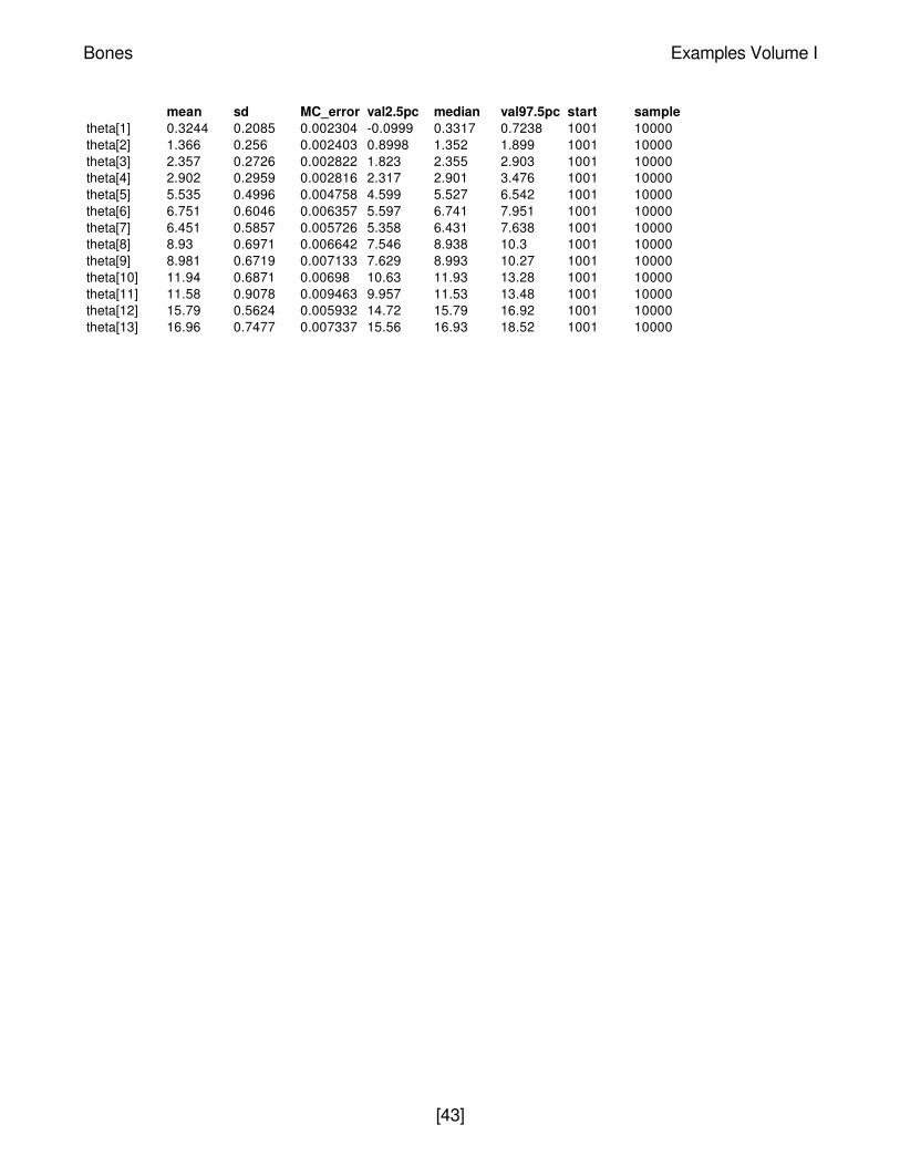
mean sd MC_error val2.5pc median val97.5pc start sampletheta[1] 0.3244 0.2085 0.002304 -0.0999 0.3317 0.7238 1001 10000theta[2] 1.366 0.256 0.002403 0.8998 1.352 1.899 1001 10000theta[3] 2.357 0.2726 0.002822 1.823 2.355 2.903 1001 10000theta[4] 2.902 0.2959 0.002816 2.317 2.901 3.476 1001 10000theta[5] 5.535 0.4996 0.004758 4.599 5.527 6.542 1001 10000theta[6] 6.751 0.6046 0.006357 5.597 6.741 7.951 1001 10000theta[7] 6.451 0.5857 0.005726 5.358 6.431 7.638 1001 10000theta[8] 8.93 0.6971 0.006642 7.546 8.938 10.3 1001 10000theta[9] 8.981 0.6719 0.007133 7.629 8.993 10.27 1001 10000theta[10] 11.94 0.6871 0.00698 10.63 11.93 13.28 1001 10000theta[11] 11.58 0.9078 0.009463 9.957 11.53 13.48 1001 10000theta[12] 15.79 0.5624 0.005932 14.72 15.79 16.92 1001 10000theta[13] 16.96 0.7477 0.007337 15.56 16.93 18.52 1001 10000
Bones Examples Volume I
[43]
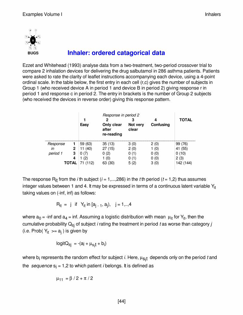
Inhaler: ordered catagorical data
Ezzet and Whitehead (1993) analyse data from a two-treatment, two-period crossover trial tocompare 2 inhalation devices for delivering the drug salbutamol in 286 asthma patients. Patientswere asked to rate the clarity of leaflet instructions accompanying each device, using a 4-pointordinal scale. In the table below, the first entry in each cell (r,c) gives the number of subjects inGroup 1 (who received device A in period 1 and device B in period 2) giving response r inperiod 1 and response c in period 2. The entry in brackets is the number of Group 2 subjects(who received the devices in reverse order) giving this response pattern.
The response Rit from the i th subject (i = 1,...,286) in the t th period (t = 1,2) thus assumesinteger values between 1 and 4. It may be expressed in terms of a continuous latent variable Yittaking values on (-inf, inf) as follows:
Rit = j if Yit in [aj - 1, aj), j = 1,..,4
where a0 = -inf and a4 = inf. Assuming a logistic distribution with mean µit for Yit, then thecumulative probability Qitj of subject i rating the treatment in period t as worse than category j(i.e. Prob( Yit >= aj ) is given by
logitQitj = -(aj + µsit + bi)
where bi represents the random effect for subject i. Here, µsit depends only on the period t and
the sequence si = 1,2 to which patient i belongs. It is defined as
µ11 = β / 2 + π / 2
Response in period 21 2 3 4 TOTAL
Easy Only clear Not very Confusingafter clearre-reading
________________________________________________________________________Response 1 59 (63) 35 (13) 3 (0) 2 (0) 99 (76)
in 2 11 (40) 27 (15) 2 (0) 1 (0) 41 (55)period 1 3 0 (7) 0 (2) 0 (1) 0 (0) 0 (10)
4 1 (2) 1 (0) 0 (1) 0 (0) 2 (3)TOTAL 71 (112) 63 (30) 5 (2) 3 (0) 142 (144)
Examples Volume I Inhalers
[44]

µ12 = -β / 2 - π / 2 - κ
µ21 = -β / 2 + π / 2
µ22 = β / 2 - π / 2 + κ
where β represents the treatment effect, π represents the period effect and κ represents thecarryover effect. The probability of subject i giving response j in period t is thus given by pitj = Qitj
- 1 - Qitj, where Qit0 = 1 and Qit4 = 0 (see also the Bones example).
The BUGS language for this model is shown below. We assume the bi's to be normallydistributed with zero mean and common precision τ. The fixed effects β, π and κ are given vaguenormal priors, as are the unknown cut points a1, a2 and a3. We also impose order constraints onthe latter using the I(,) notation in BUGS, to ensure that a1 < a2 < a3.
model{## Construct individual response data from contingency table#
for (i in 1 : Ncum[1, 1]) {group[i] <- 1for (t in 1 : T) { response[i, t] <- pattern[1, t] }
}for (i in (Ncum[1,1] + 1) : Ncum[1, 2]) {
group[i] <- 2 for (t in 1 : T) { response[i, t] <- pattern[1, t] }}
for (k in 2 : Npattern) {for(i in (Ncum[k - 1, 2] + 1) : Ncum[k, 1]) {
group[i] <- 1 for (t in 1 : T) { response[i, t] <- pattern[k, t] }}for(i in (Ncum[k, 1] + 1) : Ncum[k, 2]) {
group[i] <- 2 for (t in 1 : T) { response[i, t] <- pattern[k, t] }}
}## Model#
for (i in 1 : N) {for (t in 1 : T) {
for (j in 1 : Ncut) {## Cumulative probability of worse response than j#
Inhalers Examples Volume I
[45]

logit(Q[i, t, j]) <- -(a[j] + mu[group[i], t] + b[i])}
## Probability of response = j#
p[i, t, 1] <- 1 - Q[i, t, 1]for (j in 2 : Ncut) { p[i, t, j] <- Q[i, t, j - 1] - Q[i, t, j] }p[i, t, (Ncut+1)] <- Q[i, t, Ncut]
response[i, t] ~ dcat(p[i, t, ])}
## Subject (random) effects#
b[i] ~ dnorm(0.0, tau)}
## Fixed effects#
for (g in 1 : G) {for(t in 1 : T) {
# logistic mean for group i in period tmu[g, t] <- beta * treat[g, t] / 2 + pi * period[g, t] / 2 + kappa * carry[g, t]
}}beta ~ dnorm(0, 1.0E-06)pi ~ dnorm(0, 1.0E-06)kappa ~ dnorm(0, 1.0E-06)
# ordered cut points for underlying continuous latent variablea[1] ~ dnorm(0, 1.0E-06)I(, a[2])a[2] ~ dnorm(0, 1.0E-06)I(a[1], a[3])a[3] ~ dnorm(0, 1.0E-06)I(a[2], )
tau ~ dgamma(0.001, 0.001)sigma <- sqrt(1 / tau)log.sigma <- log(sigma)
}
Note that the data is read into BUGS in the original contigency table format to economize onspace and effort. The indivdual responses for each of the 286 patients are then constructedwithin BUGS.
Data ( click to open )
Examples Volume I Inhalers
[46]

Inits ( click to open )
Results
A 1000 update burn in followed by a further 10000 updates gave the parameter estimates
The estimates can be compared with those of Ezzet and Whitehead, who used the Newton-Raphson method and numerical integration to obtain maximum-likelihood estimates of theparameters. They reported β = 1.17 +/- 0.75, π = -0.23 +/- 0.20, κ = 0.21 +/- 0.49, logσ = 0.17 +/-0.23, a1 = 0.68, a2 = 3.85, a3 = 5.10
mean sd MC_error val2.5pc median val97.5pc start samplea[1] 0.712 0.1382 0.004156 0.4566 0.7069 0.9981 1001 10000a[2] 3.936 0.3298 0.01597 3.326 3.924 4.614 1001 10000a[3] 5.28 0.4699 0.01893 4.412 5.262 6.239 1001 10000beta 1.067 0.3199 0.008454 0.4575 1.057 1.714 1001 10000kappa 0.2463 0.2503 0.005605 -0.2394 0.2456 0.7475 1001 10000log.sigma 0.195 0.203 0.01356 -0.2494 0.2145 0.5424 1001 10000pi -0.2367 0.1976 0.002313 -0.6214 -0.238 0.1509 1001 10000sigma 1.24 0.2412 0.01562 0.7793 1.239 1.72 1001 10000
Inhalers Examples Volume I
[47]
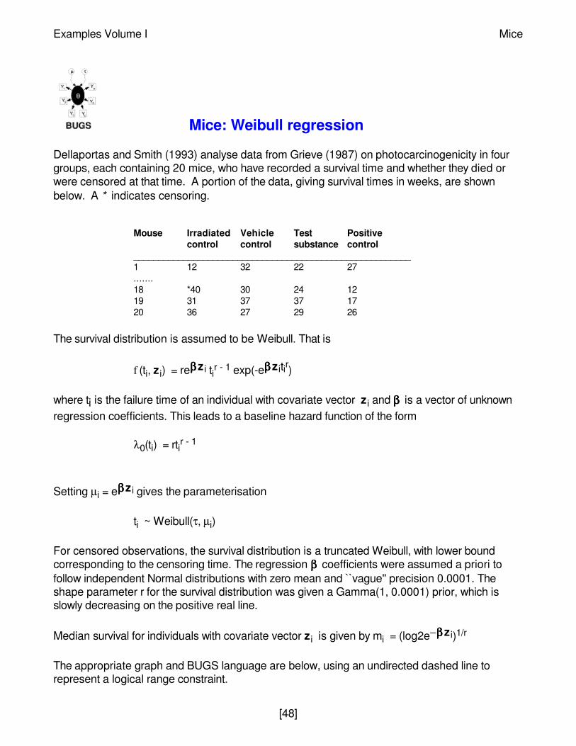
Mice: Weibull regression
Dellaportas and Smith (1993) analyse data from Grieve (1987) on photocarcinogenicity in fourgroups, each containing 20 mice, who have recorded a survival time and whether they died orwere censored at that time. A portion of the data, giving survival times in weeks, are shownbelow. A * indicates censoring.
The survival distribution is assumed to be Weibull. That is
f (ti, z i) = reββββ z i tir - 1 exp(-eββββ z itir)
where ti is the failure time of an individual with covariate vector z i and ββββ is a vector of unknownregression coefficients. This leads to a baseline hazard function of the form
λ0(ti) = rtir - 1
Setting µi = eββββ z i gives the parameterisation
ti ~ Weibull(τ, µi)
For censored observations, the survival distribution is a truncated Weibull, with lower boundcorresponding to the censoring time. The regression ββββ coefficients were assumed a priori tofollow independent Normal distributions with zero mean and ``vague'' precision 0.0001. Theshape parameter r for the survival distribution was given a Gamma(1, 0.0001) prior, which isslowly decreasing on the positive real line.
Median survival for individuals with covariate vector z i is given by mi = (log2e−ββββ z i)1/r
The appropriate graph and BUGS language are below, using an undirected dashed line torepresent a logical range constraint.
Mouse Irradiated Vehicle Test Positivecontrol control substance control
________________________________________________________1 12 32 22 27.......18 *40 30 24 1219 31 37 37 1720 36 27 29 26
Examples Volume I Mice
[48]

model{
for(i in 1 : M) {for(j in 1 : N) {
t[i, j] ~ dweib(r, mu[i])I(t.cen[i, j],)}mu[i] <- exp(beta[i])beta[i] ~ dnorm(0.0, 0.001)median[i] <- pow(log(2) * exp(-beta[i]), 1/r)
}r ~ dexp(0.001)veh.control <- beta[2] - beta[1]test.sub <- beta[3] - beta[1]pos.control <- beta[4] - beta[1]
}
We note a number of tricks in setting up this model. First, individuals who are censored are givena missing value in the vector of failure times t, whilst individuals who fail are given a zero in thecensoring time vector t.cen (see data file listing below). The truncated Weibull is modelled usingI(t.cen[i],) to set a lower bound. Second, we set a parameter beta[j] for each treatment group j.The contrasts beta[j] with group 1 (the irradiated control) are calculated at the end. Alternatively,we could have included a grand mean term in the relative risk model and constrained beta[1] tobe zero.
for(j IN 1 : N)
for(i IN 1 : M)
t[i, j]
veh.control
test.sub
pos.control
median[i]
rbeta[i]
mu[i]
t.cen[i, j]
Mice Examples Volume I
[49]

Data ( click to open )
Inits ( click to open )
Results
A burn in of 1000 updates followed by a further 10000 updates gave the parameter estimatesmean sd MC_error val2.5pc median val97.5pc start sample
median[1] 23.65 2.002 0.05203 20.06 23.54 27.93 1001 10000median[2] 35.18 3.54 0.05764 29.22 34.88 43.21 1001 10000median[3] 26.68 2.437 0.05828 22.36 26.5 31.99 1001 10000median[4] 21.28 1.849 0.03371 18.01 21.16 25.36 1001 10000pos.control 0.3088 0.3416 0.005912 -0.3644 0.3115 0.9685 1001 10000r 2.902 0.2781 0.02332 2.367 2.904 3.444 1001 10000test.sub -0.3475 0.3435 0.004663 -1.022 -0.3478 0.3185 1001 10000veh.control -1.143 0.365 0.006778 -1.87 -1.141 -0.4315 1001 10000
Examples Volume I Mice
[50]

Kidney: Weibull regression with random efects
McGilchrist and Aisbett (1991) analyse time to first and second recurrence of infection in kidneypatients on dialysis using a Cox model with a multiplicative frailty parameter for each individual.The risk variables considered are age, sex and underlying disease (coded other, GN, AN andPKD). A portion of the data are shown below.
We have analysed the same data assuming a parametric Weibull distribution for the survivorfunction, and including an additive random effect bi for each patient in the exponent of the hazardmodel as follows
tij ~ Weibull(r, µij) i = 1,...,38; j = 1,2
logµij = α + βageAGEij + βsexSEXi + βdisease1DISEASEi1 +βdisease2DISEASEi2 + βdisease3DISEASEi3 + bi
bi ~ Normal(0, τ)
where AGEij is a continuous covariate, SEXi is a 2-level factor and DISEASEik (k = 1,2,3) aredummy variables representing the 4-level factor for underlying disease. Note that the the survivaldistribution is a truncated Weibull for censored observations as discussed in the mice example.The regression coefficients and the precision of the random effects τ are given independent``non-informative'' priors, namely
bk ~ Normal(0, 0.0001)
τ ~ Gamma(0.0001, 0.0001)
Patient Recurrence Event Age at Sex DiseaseNumber time t (2 = cens) time t (1 = female) (0 = other; 1 = GN
2 = AN; 3 = PKD)______________________________________________________________________1 8,16 1,1 28,28 0 02 23,13 1,2 48,48 1 13 22,28 1,1 32,32 0 04 447,318 1,1 31,32 1 0.....35 119,8 1,1 22,22 1 136 54,16 2,2 42,42 1 137 6,78 2,1 52,52 1 338 63,8 1,2 60,60 0 3
Kidney Examples Volume I
[51]

The shape parameter of the survival distribution r is given a Gamma(1, 0.0001) prior which isslowly decreasing on the positive real line.
The graphical model and BUGS language are given below.
Graphical model for kidney example:
BUGS language for kidney example
model{
for (i in 1 : N) {for (j in 1 : M) {
# Survival times bounded below by censoring times:t[i,j] ~ dweib(r, mu[i,j]) I(t.cen[i, j], );log(mu[i,j ]) <- alpha + beta.age * age[i, j]
+ beta.sex *sex[i]+ beta.dis[disease[i]] + b[i];
}# Random effects:
b[i] ~ dnorm(0.0, tau)}
# Priors:alpha ~ dnorm(0.0, 0.0001);
for(j IN 1 : M)
for(i IN 1 : N)
alpha beta.dis[4]beta.dis[3]beta.dis[2]beta.sexbeta.age
sigma
tau
b[i]
r
t.cen[i, j]
mu[i, j]
t[i, j]
Examples Volume I Kidney
[52]
beta.age ~ dnorm(0.0, 0.0001);beta.sex ~ dnorm(0.0, 0.0001);
# beta.dis[1] <- 0; # corner-point constraintfor(k in 2 : 4) {
beta.dis[k] ~ dnorm(0.0, 0.0001);}tau ~ dgamma(1.0E-3, 1.0E-3);r ~ dgamma(1.0, 1.0E-3);sigma <- 1 / sqrt(tau); # s.d. of random effects
}
Data ( click to open )
Inits ( click to open )
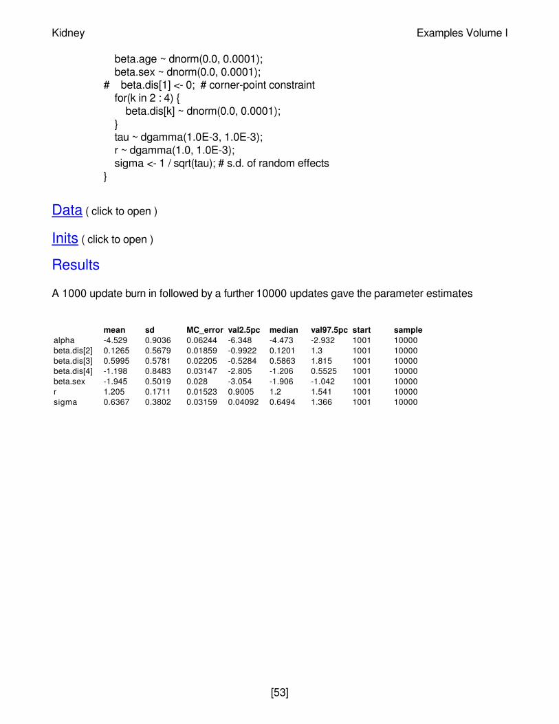
Results
A 1000 update burn in followed by a further 10000 updates gave the parameter estimates
mean sd MC_error val2.5pc median val97.5pc start samplealpha -4.529 0.9036 0.06244 -6.348 -4.473 -2.932 1001 10000beta.dis[2] 0.1265 0.5679 0.01859 -0.9922 0.1201 1.3 1001 10000beta.dis[3] 0.5995 0.5781 0.02205 -0.5284 0.5863 1.815 1001 10000beta.dis[4] -1.198 0.8483 0.03147 -2.805 -1.206 0.5525 1001 10000beta.sex -1.945 0.5019 0.028 -3.054 -1.906 -1.042 1001 10000r 1.205 0.1711 0.01523 0.9005 1.2 1.541 1001 10000sigma 0.6367 0.3802 0.03159 0.04092 0.6494 1.366 1001 10000
Kidney Examples Volume I
[53]

Leuk: Cox regression
Several authors have discussed Bayesian inference for censored survival data where theintegrated baseline hazard function is to be estimated non-parametrically Kalbfleisch (1978),Kalbfleisch and Prentice (1980), Clayton (1991), Clayton (1994).Clayton (1994) formulates theCox model using the counting process notation introduced by Andersen and Gill (1982) anddiscusses estimation of the baseline hazard and regression parameters using MCMC methods.Although his approach may appear somewhat contrived, it forms the basis for extensions torandom effect (frailty) models, time-dependent covariates, smoothed hazards, multiple eventsand so on. We show below how to implement this formulation of the Cox model in BUGS.
For subjects i = 1,...,n, we observe processes Ni(t) which count the number of failures which haveoccurred up to time t. The corresponding intensity process Ii(t) is given by
Ii(t)dt = E(dNi(t) | Ft-)
where dNi(t) is the increment of Ni over the small time interval [t, t+dt), and Ft- represents theavailable data just before time t. If subject i is observed to fail during this time interval, dNi(t) willtake the value 1; otherwise dNi(t) = 0. Hence E(dNi(t) | Ft-) corresponds to the probability ofsubject i failing in the interval [t, t+dt). As dt -> 0 (assuming time to be continuous) then thisprobability becomes the instantaneous hazard at time t for subject i. This is assumed to have theproportional hazards form
Ii(t) = Yi(t)λ0(t)exp(ββββ z i)
where Yi(t) is an observed process taking the value 1 or 0 according to whether or not subject i isobserved at time t and λ0(t)exp(ββββ z i) is the familiar Cox regression model. Thus we haveobserved data D = Ni(t), Yi(t), z i; i = 1,..n and unknown parameters ββββ and Λ0(t) = Integral(λ0(u), u,t, 0), the latter to be estimated non-parametrically.
The joint posterior distribution for the above model is defined by
P(ββββ , Λ0() | D) ~ P(D | ββββ , Λ0()) P(ββββ ) P(Λ0())
For BUGS, we need to specify the form of the likelihood P(D | ββββ , Λ0()) and prior distributions forββββ and Λ0(). Under non-informative censoring, the likelihood of the data is proportional to
n
Examples Volume I Leuk
[54]

Π[Π Ιi(t)dNi(t)] exp(- Ii(t)dt)i = 1 t >= 0
This is essentially as if the counting process increments dNi(t) in the time interval [t, t+dt) areindependent Poisson random variables with means Ii(t)dt:
dNi(t) ~ Poisson(Ii(t)dt)
We may write
Ii(t)dt = Yi(t)exp(ββββ z i)dΛ0(t)
where dΛ0(t) = Λ0(t)dt is the increment or jump in the integrated baseline hazard functionoccurring during the time interval [t, t+dt). Since the conjugate prior for the Poisson mean is thegamma distribution, it would be convenient if Λ0() were a process in which the increments dΛ0(t)are distributed according to gamma distributions. We assume the conjugate independentincrements prior suggested by Kalbfleisch (1978), namely
dΛ0(t) ~ Gamma(cdΛ∗0(t), c)
Here, dΛ∗0(t) can be thought of as a prior guess at the unknown hazard function, with c
representing the degree of confidence in this guess. Small values of c correspond to weak priorbeliefs. In the example below, we set dΛ∗
0(t) = r dt where r is a guess at the failure rate per unittime, and dt is the size of the time interval.
The above formulation is appropriate when genuine prior information exists concerning theunderlying hazard function. Alternatively, if we wish to reproduce a Cox analysis but with, say,additional hierarchical structure, we may use the multinomial-Poisson trick described in theBUGS manual. This is equivalent to assuming independent increments in the cumulative `non-informative' priors. This formulation is also shown below.
The fixed effect regression coefficients ββββ are assigned a vague prior
β ~ Normal(0.0, 0.000001)
BUGS language for the Leuk example:
model{# Set up data
for(i in 1:N) {for(j in 1:T) {
Leuk Examples Volume I
[55]

# risk set = 1 if obs.t >= tY[i,j] <- step(obs.t[i] - t[j] + eps)
# counting process jump = 1 if obs.t in [ t[j], t[j+1] )# i.e. if t[j] <= obs.t < t[j+1]
dN[i, j] <- Y[i, j] * step(t[j + 1] - obs.t[i] - eps) * fail[i]}
}# Model
for(j in 1:T) {for(i in 1:N) {
dN[i, j] ~ dpois(Idt[i, j]) # LikelihoodIdt[i, j] <- Y[i, j] * exp(beta * Z[i]) * dL0[j] # Intensity
}dL0[j] ~ dgamma(mu[j], c)mu[j] <- dL0.star[j] * c # prior mean hazard
# Survivor function = exp(-Integral{l0(u)du})^exp(beta*z)S.treat[j] <- pow(exp(-sum(dL0[1 : j])), exp(beta * -0.5));S.placebo[j] <- pow(exp(-sum(dL0[1 : j])), exp(beta * 0.5));
}c <- 0.001r <- 0.1for (j in 1 : T) {
dL0.star[j] <- r * (t[j + 1] - t[j])}beta ~ dnorm(0.0,0.000001)
}
Data ( click to open )
Inits ( click to open )
Results
A 1000 update burn in followed by a further 10000 updates gave the parameter estimates
Examples Volume I Leuk
[56]
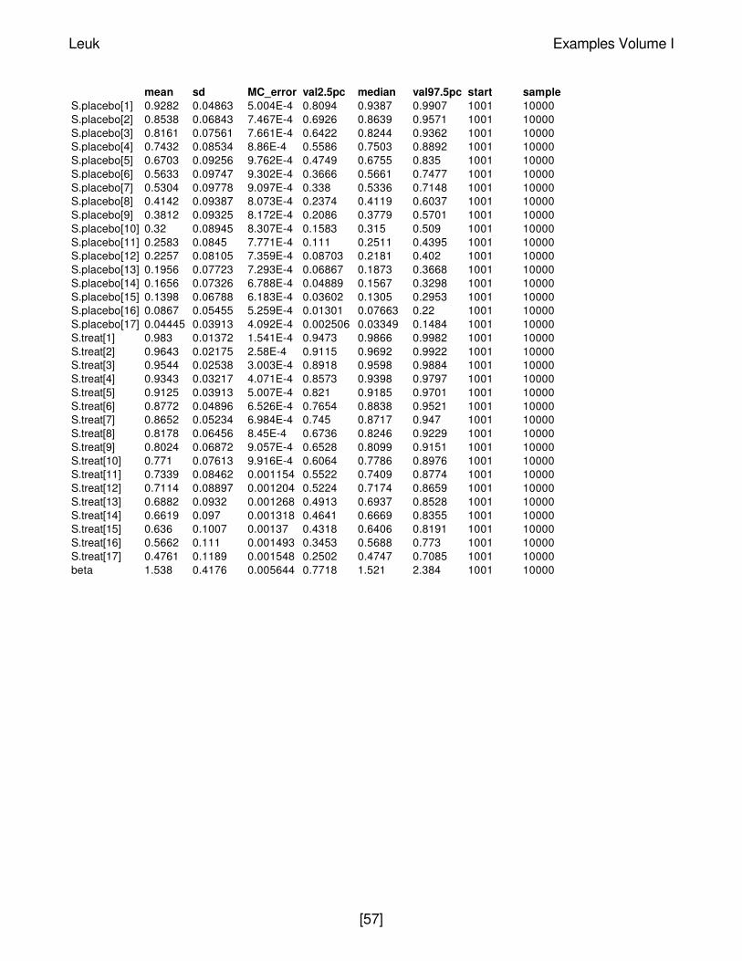
mean sd MC_error val2.5pc median val97.5pc start sampleS.placebo[1] 0.9282 0.04863 5.004E-4 0.8094 0.9387 0.9907 1001 10000S.placebo[2] 0.8538 0.06843 7.467E-4 0.6926 0.8639 0.9571 1001 10000S.placebo[3] 0.8161 0.07561 7.661E-4 0.6422 0.8244 0.9362 1001 10000S.placebo[4] 0.7432 0.08534 8.86E-4 0.5586 0.7503 0.8892 1001 10000S.placebo[5] 0.6703 0.09256 9.762E-4 0.4749 0.6755 0.835 1001 10000S.placebo[6] 0.5633 0.09747 9.302E-4 0.3666 0.5661 0.7477 1001 10000S.placebo[7] 0.5304 0.09778 9.097E-4 0.338 0.5336 0.7148 1001 10000S.placebo[8] 0.4142 0.09387 8.073E-4 0.2374 0.4119 0.6037 1001 10000S.placebo[9] 0.3812 0.09325 8.172E-4 0.2086 0.3779 0.5701 1001 10000S.placebo[10] 0.32 0.08945 8.307E-4 0.1583 0.315 0.509 1001 10000S.placebo[11] 0.2583 0.0845 7.771E-4 0.111 0.2511 0.4395 1001 10000S.placebo[12] 0.2257 0.08105 7.359E-4 0.08703 0.2181 0.402 1001 10000S.placebo[13] 0.1956 0.07723 7.293E-4 0.06867 0.1873 0.3668 1001 10000S.placebo[14] 0.1656 0.07326 6.788E-4 0.04889 0.1567 0.3298 1001 10000S.placebo[15] 0.1398 0.06788 6.183E-4 0.03602 0.1305 0.2953 1001 10000S.placebo[16] 0.0867 0.05455 5.259E-4 0.01301 0.07663 0.22 1001 10000S.placebo[17] 0.04445 0.03913 4.092E-4 0.002506 0.03349 0.1484 1001 10000S.treat[1] 0.983 0.01372 1.541E-4 0.9473 0.9866 0.9982 1001 10000S.treat[2] 0.9643 0.02175 2.58E-4 0.9115 0.9692 0.9922 1001 10000S.treat[3] 0.9544 0.02538 3.003E-4 0.8918 0.9598 0.9884 1001 10000S.treat[4] 0.9343 0.03217 4.071E-4 0.8573 0.9398 0.9797 1001 10000S.treat[5] 0.9125 0.03913 5.007E-4 0.821 0.9185 0.9701 1001 10000S.treat[6] 0.8772 0.04896 6.526E-4 0.7654 0.8838 0.9521 1001 10000S.treat[7] 0.8652 0.05234 6.984E-4 0.745 0.8717 0.947 1001 10000S.treat[8] 0.8178 0.06456 8.45E-4 0.6736 0.8246 0.9229 1001 10000S.treat[9] 0.8024 0.06872 9.057E-4 0.6528 0.8099 0.9151 1001 10000S.treat[10] 0.771 0.07613 9.916E-4 0.6064 0.7786 0.8976 1001 10000S.treat[11] 0.7339 0.08462 0.001154 0.5522 0.7409 0.8774 1001 10000S.treat[12] 0.7114 0.08897 0.001204 0.5224 0.7174 0.8659 1001 10000S.treat[13] 0.6882 0.0932 0.001268 0.4913 0.6937 0.8528 1001 10000S.treat[14] 0.6619 0.097 0.001318 0.4641 0.6669 0.8355 1001 10000S.treat[15] 0.636 0.1007 0.00137 0.4318 0.6406 0.8191 1001 10000S.treat[16] 0.5662 0.111 0.001493 0.3453 0.5688 0.773 1001 10000S.treat[17] 0.4761 0.1189 0.001548 0.2502 0.4747 0.7085 1001 10000beta 1.538 0.4176 0.005644 0.7718 1.521 2.384 1001 10000
Leuk Examples Volume I
[57]

LeukFr: Cox regression with random effects
Freireich et al (1963)'s data presented in the Leuk example actually arise via a paired design.Patients were matched according to their remission status (partial or complete). One patientfrom each pair received the drug 6-MP whilst the other received the placebo. We may introducean additional vector (called pair) in the BUGS data file to indicate each of the 21 pairs ofpatients.
We model the potential 'clustering' of failure times within pairs of patients by introducing a group-specific random effect or frailty term into the proportional hazards model. Using the countingprocess notation introduced in the Leuk example, this gives
Ii (t) dt = Yi (t) exp( β ' zi + bpairi ) dΛ0(t) i = 1,...,42; pairi = 1,...,21bpairi ~ Normal(0, τ)
A non-informative Gamma prior is assumed for τ, the precision of the frailty parameters. Notethat the above 'additive' formualtion of the frailty model is equivalent to assuming multiplicativefrailties with a log-Normal population distibution. Clayton (1991) discusses the Cox proportionalhazards model with multiplicative frailties, but assumes a Gamma population distribution.
The modified BUGS code needed to include a fraility term in the Leuk example is shown below
model{# Set up data
for(i in 1 : N) {for(j in 1 : T) {
# risk set = 1 if obs.t >= tY[i, j] <- step(obs.t[i] - t[j] + eps)
# counting process jump = 1 if obs.t in [ t[j], t[j+1] )# i.e. if t[j] <= obs.t < t[j+1]
dN[i, j] <- Y[i, j ] *step(t[j+1] - obs.t[i] - eps)*fail[i]}
}# Model
for(j in 1 : T) {for(i in 1 : N) {
dN[i, j] ~ dpois(Idt[i, j])Idt[i, j] <- Y[i, j] * exp(beta * Z[i]+b[pair[i]]) * dL0[j]
}dL0[j] ~ dgamma(mu[j], c)
Examples Volume I Leukfr
[58]
mu[j] <- dL0.star[j] * c # prior mean hazard# Survivor function = exp(-Integral{l0(u)du})^exp(beta * z)
S.treat[j] <- pow(exp(-sum(dL0[1 : j])), exp(beta * -0.5))S.placebo[j] <- pow(exp(-sum(dL0[1 : j])), exp(beta * 0.5))
}for(k in 1 : Npairs) {
b[k] ~ dnorm(0.0, tau);}tau ~ dgamma(0.001, 0.001)sigma <- sqrt(1 / tau)c <- 0.001 r <- 0.1for (j in 1 : T) {
dL0.star[j] <- r * (t[j+1]-t[j])}beta ~ dnorm(0.0,0.000001)
}
Data ( click to open )
Inits ( click to open )
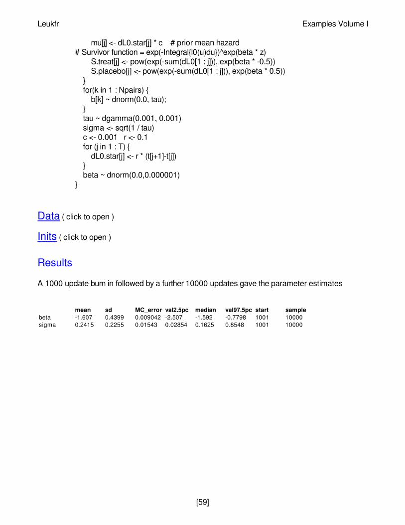
Results
A 1000 update burn in followed by a further 10000 updates gave the parameter estimates
mean sd MC_error val2.5pc median val97.5pc start samplebeta -1.607 0.4399 0.009042 -2.507 -1.592 -0.7798 1001 10000sigma 0.2415 0.2255 0.01543 0.02854 0.1625 0.8548 1001 10000
Leukfr Examples Volume I
[59]