the brasília experiment - the world bankdocuments.worldbank.org/.../pdf/wps6964.pdf · the...
TRANSCRIPT

Policy Research Working Paper 6964
The Brasília Experiment
Road Access and the Spatial Pattern of Long-term Local Development in Brazil
Julia Bird Stéphane Straub
Development Economics Vice PresidencyDevelopment Policy DepartmentJuly 2014
WPS6964P
ublic
Dis
clos
ure
Aut
horiz
edP
ublic
Dis
clos
ure
Aut
horiz
edP
ublic
Dis
clos
ure
Aut
horiz
edP
ublic
Dis
clos
ure
Aut
horiz
edP
ublic
Dis
clos
ure
Aut
horiz
edP
ublic
Dis
clos
ure
Aut
horiz
edP
ublic
Dis
clos
ure
Aut
horiz
edP
ublic
Dis
clos
ure
Aut
horiz
ed

Produced by the Research Support Team
Abstract
The Policy Research Working Paper Series disseminates the findings of work in progress to encourage the exchange of ideas about development issues. An objective of the series is to get the findings out quickly, even if the presentations are less than fully polished. The papers carry the names of the authors and should be cited accordingly. The findings, interpretations, and conclusions expressed in this paper are entirely those of the authors. They do not necessarily represent the views of the International Bank for Reconstruction and Development/World Bank and its affiliated organizations, or those of the Executive Directors of the World Bank or the governments they represent.
Policy Research Working Paper 6964
This paper is a product of the Development Policy Department, Development Economics Vice Presidency. It is part of a larger effort by the World Bank to provide open access to its research and make a contribution to development policy discussions around the world. Policy Research Working Papers are also posted on the Web at http://econ.worldbank.org. The authors may be contacted at [email protected] and [email protected].
This paper studies the impact of the rapid expansion of the Brazilian road network, which occurred from the 1960s to the 2000s, on the growth and spatial allocation of population and economic activity across the country’s municipalities. It addresses the problem of endogeneity in infrastructure loca-tion by using an original empirical strategy, based on the
“historical natural experiment” constituted by the creation of the new federal capital city Brasília in 1960. The results
reveal a dual pattern, with improved transport connections increasing concentration of economic activity and popula-tion around the main centers in the South of the country, while spurring the emergence of secondary economic cen-ters in the less developed North, in line with predictions in terms of agglomeration economies. Over the period, roads are shown to account for half of pcGDP growth and to spur a significant decrease in spatial inequality.

The Brasília Experiment:
Road Access and the Spatial Pattern of Long-term Local
Development in Brazil
Julia Bird∗and Stéphane Straub†
∗Toulouse School of economics, Arqade. contact: [email protected].†Toulouse School of economics, Arqade, IDEI and IAST. contact: [email protected].
We thank Nicolas Ahmed-Michaux-Bellaire for excellent research assistance, and EmmanuelleAuriol, Jean-Jacques Dethier, Pascaline Dupas, Marcel Fafchamps, Claudio Ferraz, Fred Finan,Somik Lall, Rocco Macchiavello, Marti Mestieri, Guy Michaels, Nancy Qian, Jean-LaurentRosenthal, Adam Storeygard, and participants in seminars in Berkeley, EUDN Berlin, Stanford,Toulouse, Universidad de Chile and the World Bank for helpful discussion. Support from theWorld Bank Research Support Budget is gratefully acknowledged.

1 Introduction
Brasília, Brazil's current federal capital city, was built from scratch between 1956
and 1960, in a previously unpopulated area selected because of its geographic
centrality, at the initiative of then President Juscelino Kubitschek, who wanted
to shift the country's center of gravity away from the Southern coastal region.
The following decades were also characterized by one of the largest post war
infrastructure development program worldwide, as Brazil paved over 150,000 km
of roads.1
An important share of this national road construction program was geared
towards connecting the new capital to other main population and economic cen-
ters. The resulting radial highway system also incidentally connected other inland
municipalities along the way. Proximity to the roads built after the creation of
Brasília was a key factor in explaining the subsequent changes in local access to
major economic centers. However, whether municipalities were close to or far from
the new corridors was mostly due to luck rather than to their speci�c economic
or geographic characteristics.
We exploit this �historical natural experiment� to study the impact of the
rapid expansion of the Brazilian road network on the growth and spatial allo-
cation of population and economic activity across the country's municipalities
between 1970 and 2000. This allows us to solve the main di�culty inherent to
eliciting the impact of roads, namely their potential non random placement. In-
deed, roads are likely to be allocated to speci�c locations according to observed
or unobserved characteristics that are not orthogonal to their development po-
tential. For example, they may be prioritized in fast growing municipalities or
in those with suitable geographic characteristics, in which case their estimated
impact would be upwardly biased. Alternatively, policymakers may want to cater
to the needs of lagging regions, with opposite e�ects. Finally, examples of in-
frastructure works allocated for political reasons rather than economic rationales
abound,2 potentially biasing estimates towards zero.
Our empirical strategy is based on superimposing onto a map of Brazil eight
1Mitchell (1995) and World Bank (2008). This �gure excludes urban roads.2See for example Cadot, Roller and Stephan (2006) and Burgess et al. (2013).
2

straight lines, coinciding with the subsequent shape of the radial highway sys-
tem, which connect the country's new capital to State capitals and ports chosen
according to their population size and economic importance in 1956, the year
of the decision to build Brasília. We then create a municipality-level distance
index capturing proximity to the lines, and use it to instrument the subsequent
municipality-level improvement in road access over time, and assess its impact on
local-level changes in population and GDP, as well as GDP per capita. Our main
results exploit successive census data between 1970 and 2000, aggregated at the
municipality level, together with a composite measure of the cost of access from
each individual location to its State capital in each decade from the late 1960s to
the 1990s.
After developing a simple theoretical framework, we present three sets of re-
sults. First, the e�ect of road access improvements on population and GDP
supports a story of a dual geographical pattern. In the more developed Southern
part of Brazil, improvements in travel costs resulted in a growing concentration
of population and economic activity in large radiuses of up to several hundreds
kilometers around the main urban areas. The population movements were clearly
quantitatively more important than the spatial changes in GDP and GDP per
capita. Northern State capitals underwent the opposite process, with reductions
in travel costs spurring a concentration of population and economic activity away
from the main urban centers, therefore generating the emergence of numerous
secondary urban centers. Finally, the spatial impacts on GDP and population
roughly balanced, meaning that the net e�ect on GDP per capita appears mostly
insigni�cant.
Second, we show that this dual pattern can be explained by variations in
road endpoints along a number of characteristics that proxy for the agglomer-
ation economies described in the urban literature. As predicted by our model,
an improvement of road infrastructure, through the implied reduction in e�ective
distance, spurs agglomeration towards urban areas if these have a high enough
wage rental ratio, which happens if they are large enough, have a high stock of
human capital, a high industry to service ratio, and good amenities. The opposite
dispersion process occurs otherwise.
3

Third, we relate the municipality-level marginal e�ects of road access improve-
ments to the relative size of these locations as compared to the endpoints on the
relevant line connecting them. Again, a dual pattern appears. In the South it is
the smaller municipalities that gain the most from reduced access costs. There is
therefore a combination of induced spatial dispersion, in the sense of the spatial
growth literature, together with a home market e�ect-like geographical concentra-
tion process, as these small locations are mostly located around the main urban
centers. On the other hand, the results for the North show a positive impact of
better road access for a group of approximately 30 large municipalities, indicating
spatial concentration, together with geographical dispersion, as these locations
are intermediate size cities away from the main urban centers.
Finally, our results indicate that the causal growth e�ect of the radial highway
network development for the country was huge, accounting for almost half of
the 136% growth in per capita GDP over the period, and that the geographical
redistribution e�ects were important. Looking at changes in the spatial Gini
coe�cient across municipalities and regions, we estimate that spatial inequality
was signi�cantly reduced particularly due to positive growth impacts in the North
and Center West.
This paper adds to a recent strand of literature that tackles the issue of trans-
portation infrastructure impact using spatially disaggregated data. First it is
related to contributions that have found evidence of speci�c positive impacts of
infrastructure access on a number of development outcomes, such as trade (Don-
aldson, 2010; Michaels, 2008), �rms' growth and e�ciency (Datta, 2012; Ghani,
Goswami and Kerr, 2013), urban growth (Duranton and Turner, 2011), popula-
tion (Atack et al., 2009), land values (Donaldson and Hornbeck, 2012) and income
levels (Storeygard, 2012, Banerjee, Du�o and Qian, 2012).3 This last paper was
the �rst one to use straight lines based on historical preconditions to provide an
exogenous measure of access to modern transportation corridors.
However, the quality of the Brazilian data allows us to innovate by using the
3More broadly, our paper also relates to the literature that uses Brazil as a testing groundfor the link between improvements in di�erent types of infrastructure and economic outcomes,including Lipscomb, Mobarak and Barham (2013) on electricity, and Chein and Assuncao (2009)on roads, migration and labor markets, and Da Mata et al. (2007) on city growth.
4

measures of distance to the lines to instrument the time-varying cost of access
variables, which capture both the distance and the quality of connections to the
country's main economic centers. Doing this allows us to derive the causal e�ect
of the improvement in road access that followed the development of the radial
highway system, and to produce the overall counterfactual growth estimates men-
tioned above.
Our work also relates to a growing body of applied work that analyzes the
impact of transportation investment on the changes in location patterns of agents
and economic activity by integrating insights from economic geography models
(Lall et al.,2004 and 2009; Roberts et al., 2012; Baum-Snow, 2007; Baum-Snow
et al., 2013; Faber, 2012). We add to these strands of literature by being able
to provide an unprecedented view into the long-run transformation of a large
emerging country through the analysis of a longer period (30 years) than studied
before, and by looking at the within-municipalities e�ects of improvements in
access over time, thus providing results on the local-level country-wide changes in
the distribution of outcomes.
Finally, by looking at the relationship between the impact of road improve-
ments and the spatial characteristics of each location, it also relates to the work on
spatial development of Desmet and Rossi-Hansberg (2009, 2014). In doing so, we
e�ectively combine insights from the infrastructure literature that uses spatially
disaggregated data and looks at the geography of infrastructure impacts, with
those from the spatial development literature that characterizes spatial e�ects in
terms of concentration / dispersion of activities across locations of di�erent sizes.
Our analysis highlights the long term center-periphery agglomeration e�ects
determining population movements and GDP growth across the whole Brazilian
territory, over a period in which the world's �fth largest country went from being
a low income to an upper middle income country. Our �ndings are important
because they illustrate the conditions shaping varying geographical concentra-
tion e�ects, resulting in very di�erent long-term development patterns and policy
implications of similar investments across space.
The paper is structured as follows. Section 2 develops a simple theoretical
framework to guide our empirical exercise. Section 3 details the state of Brazil-
5

ian infrastructure since the 1960s and the relevant institutional facts. Section 4
presents the di�erent sources of data used in the paper. Section 5 introduces the
empirical strategy and discusses the validity of the instrumental approach. Section
6 presents the main results and a number of robustness tests. Section 7 develops
the implications for spatial vs. geographical development. Section 8 presents the
growth counterfactual computations. Section 9 concludes. Additional material,
results, and robustness checks are provided in the Appendix.
2 A Simple Model
Consider the following simple model, which breeds two main ingredients: a basic
production function framework inspired from Banerjee et al. (2012), and insights
from the urban literature on how agglomeration economies determine the strength
of urban areas' pull factors.
There are two regions, the Center and the Periphery denoted by subscript
i ∈ {c, p}. Each region is populated by ni �rms of similar size, which produce a
tradable good using labor Li and capital Ki. Total regional output is then given
by Yi = AiKαi L
1−αi , where A is the usual technological progress term. Factors
of productions verify Lc + Lp = L and Kc + Kp = K, where L and K are total
national endowments.
Assume that all technological progress takes place in the center,4 so that Ac =
A0(Kc
)βc, where Kc = Kc
nc, and Ap = A0 (i.e., βp = 0). One interpretation is that
the Center represents an urban area with corresponding agglomeration economies
to be de�ned below, while the Periphery encompasses surrounding rural areas
where only traditional production techniques are used.
All goods and factors are mobile across regions at a cost, and we model this
process following Banerjee et al. (2012). We assume that goods move at a cost,
related to distance d, with dc = 0 and dp ≡ d > 0, so that the price of the tradable
good is p in the Center and p(1 − d) in the Periphery. Denoting by rc and wc
the rental rate of capital and the wage in the Center, the cost of moving factors
4This is without loss of generality. The important assumption is that technological progressis higher in the center.
6

across space can be formalized by assuming that the corresponding values in the
Periphery are rp = (1 − ρd)rc and wp = (1 − ηd)wc respectively. Thus, η and ρ
parametrize the size of the discounts on the price of factors that stem from the
combination of distance and productivity di�erences between the Center and the
Periphery.
Maximizing pro�t in each region, and plugging the resulting KLrelationship
into the regional production function yields (derivations are detailed in the Ap-
pendix):
YiLi
=
[(1− ηd)wc(1− ρd)rc
α
1− α
]α+βiLβii . (1)
In the spirit of the urban literature, factors will move across space until the
utility per worker is equalized across locations. Formally, we consider that the
product per worker is equalized across space, so YcLc
= YpLp. This will be the case if
for example workers own the �rms in their region, and all pro�ts are redistributed
as dividends.
Combining (1) for all i, and using the fact that Lc + Lp = L and βp = 0, we
obtain:
Lc =
[(1− ηd)wc(1− ρd)rc
α
1− α
]−1. (2)
We are interested in the comparative statics with respect to d. It is straight-
forward to observe that the sign of the derivative of the right hand side depends
on the sign of ρ− η. The following proposition states the main results of interest
for our empirical exercise.
Proposition 1 ∂Lc
∂d≥ 0 (resp. ≤) if and only if ρ ≥ η (resp. ≤). This also
implies that ∂Yc∂d≥ 0 (resp. ≤) if and only if ρ ≥ η (resp. ≤).
Intuitively, when d goes down, which can be for example thought of as a
reduction in e�ective distance resulting from the construction of new or better
roads, agglomeration in the Center occurs if the relative moving costs of factors
are such that capital moves more freely than labor. Straightforward computations
show that, given the assumptions on relative prices of factors between the Center
7

and the Periphery, this condition can be reformulated in terms of relative wage-
rental price ratios:
ρ ≤ η ⇐⇒ wcrc≥ wp
rp.
This means that there will be agglomeration in the Center if the wage-rental
price ratio is higher there. To �esh out what drives the relative level of this ratio,
consider the conditions that determine the relative opportunity cost of factors in
the urban growth literature.5
The productivity of labor and the wage-rental price ratio will be higher in
metropolitan areas that are larger, as measured by population or output, and
exhibit a high industry to service ratio. These are precisely the settings in which,
at least during early stages of development, urban externalities have been shown
to be stronger.6 In the Marshallian approach, these aspects may be thought of
as capturing labor market pooling and input sharing channels. Moreover, we
expect a higher relative wage in cities with better human capital and higher costs
of living as determined by better quality amenities. These again can be related
directly to other classical motives for external economies. The �rst one relates to
knowledge spillovers, found in cities with better human capital, while the second
one is connected to urban areas with better amenities having less of the urban
diseconomies generally associated with large cities, such as congestion and poor
infrastructure.7
Let us denote the factors mentioned above by S for city size, H the aver-
age level of human capital, IndServ
the industry-service ratio, and M the quality of
amenities. The link between agglomeration economies and these parameters then
leads to the following corollary.
Corollary 2 There exist thresholds S∗, H∗, IndServ
∗, and M∗, above which (resp.
below which) ρ ≤ η and ∂Lc
∂d≤ 0 (resp. ρ ≥ η and ∂Lc
∂d≥ 0), i.e., above which there
5See for example Rosenthal and Strange (2004), and Duranton and Puga (2013).6Henderson (2010).7These agglomeration economies could be built into the model by assuming for example that
that they a�ect technical change directly. As will become clear below, technical change stillplays a role in this model, as in its absence, labor would not move at all.
8

is agglomeration (resp. dispersion) in the Center as a result of a fall in transport
costs.
This indicates that the improvement of road infrastructure and the subsequent
reduction in transport costs is likely to spur agglomeration in cities which are large
enough, have a high stock of human capital, a high industry to service ratio, and
good amenities. In our empirical exercise below, we will establish when there is
agglomeration vs. dispersion around main urban centers in the Brazilian case, and
test directly for the determinants of these alternative patterns of agglomeration,
and for the existence of the thresholds characterized in the Corollary.
3 Brazilian Infrastructure
Brazil is South America's �rst, and the world's �fth largest country, both by
geographical area (over 8.5 million km2) and by population (close to 200 million).
As of 2008, it had just over 1.7 million kilometers of roads, around 10 kilometers
per thousand habitants, of which only 12% were paved and close to one third
concentrated in the Southeast Region. The road sector, especially the highway
system, has historically been the primary internal mode of transport for both
freight and passengers in Brazil. According to computation by Castro (2004), as
of 1999 truck transport by road represented 82.1% of domestic freight output, and
93.6% of related expenses. Over 60% of cargo was transported by road in 2011.8
Between 1952, which corresponds to the earliest available aggregate paved road
data, and 2000, there was a 471% increase in total road length. In the same period,
GDP grew by 883%. This development of the road network was accompanied by
a surge in the number of vehicles available, which went from around 6 vehicles
per thousand habitants in 1945, to 37 in 1970, then more than doubled to 84 in
the 1970-1980 decade, reaching 135 in 2000 and 219 in 2011.9
While in the 1950s, most new connections were between State capitals along
the Atlantic coast, from the 1960s, new penetration corridors started linking the
8See http://www.brasil.gov.br/sobre/tourism/infrastructure/roads, Revista CNT no.206novembro 2012
9Mitchell (1995), Ipea data.
9

hinterland main urban centers, e.g., connecting Brasília to São Paulo, Belo Hori-
zonte or Belém.10
Concomitantly, there was a rapid expansion of the agricultural frontier towards
the center-west part of the country, and an increase in the output share of the
three less developed macroregions (North, Northeast and Center-west), which
went from 17.3% in 1975 to 24% in 1996.
The country's extension and geographical dispersion implies that for munici-
palities in regions distant from the country's economic core (the States of Minas
Gerais, São Paulo and Rio de Janeiro), access to the local State capital may be
more important than access to São Paulo, which in many cases would be several
thousands of kilometers away. However, it also remains a quite centralized coun-
try. The Southeast region still represents around 60% of overall GDP, and as of
the early 2000s the port of Santos, in the State of São Paulo, accounted for 38%
of all import and export activity going through Brazilian ports, serving 13 States
almost exclusively and part of the commerce of all 27 States, and moving close to
6.5% of the country's GDP (World Bank, 2008).
As a result, we expect the strength of the pull factor exerted by metropolitan
areas to di�er across the country's main regions. In the main text, we therefore
use changes in the cost of access to the local State capitals as our main explana-
tory variable, and report results for the whole country, as well as those broken
down between South (South, Southeast) and North Brazil (North, Northeast and
Center-west). In the Appendix, we also report results using as an alternative
measure the cost of access to São Paulo.
4 Data
4.1 Census Data
Brazil is divided into 5 regions, containing 26 states and the federal district of
Brasília, which in turn contain (in 2010) 5,564 municipalities. Our analysis fo-
cuses on the impacts of road access at the municipality level, the smallest level
10Castro (2004) and World Bank (2008).
10

of government and administration within Brazil. Municipalities are based around
an urban area, from which they take their name and where their government is
based. If a secondary urban area grows within the municipality, it often divides
into two, leading to a large increase in the number of municipalities over the last
50 years: between 1960 and 2010 their number has increased from 2,767 to today's
5,564.
To ensure that the geographical focus of our data is consistent over time,
we therefore use Minimal Comparable Areas (MCAs), a geographical division of
Brazil created by the Institute of Applied Economic Research (IPEA).11 MCAs
aggregate municipalities into the smallest possible groupings, such that the bound-
aries of these groups do not change over time. The speci�c geographical unit used
is AMC 70-00, which covers 3,599 areas, allowing us to compare data at any point
between 1970 and 2000.12
The Brazilian Institute of Geography and Statistics (IBGE) holds records from
the decennial national census, which provides much of our data requirements.
From the censuses between 1970 and 2000, we extracted economic and social data
at the MCA, state, and regional level. This data includes local GDP measures,
aggregated and by main sectors,13 access to infrastructure services such as elec-
tricity, drinking water, and toilets, population �gures, and development outcomes
such as literacy rates and health indicators.
In addition, we use geographical data from IBGE's 1998 Brazilian CIM map
(International map of the world at the millionth scale) which was digitized in
2003. This map provides detailed geological and geographical coverage of Brazil,
as well the locations of cities and smaller population centers, road infrastructure
and ports. From this we were able to locate the major economic centers of 1956,
and construct lines from them leading to Brasília. By imposing the geographical
boundaries of our MCAs we could then construct an index to measure how close
11IPEA is a federal public Foundation linked to the secretariat of Strategic A�airs of thePresidency of the Republic of the Brazil.
12In what follows, we use the terms municipalities and MCAs indistinctly to mean AMC 70-00, unless speci�ed otherwise. In the robustness section, we also use an alternative grouping,AMC 40-00, to conduct pre-treatment tests.
13A detailed description of how the municipality-level production data was constructed canbe found in the Appendix.
11

each MCA is to these lines. More detail is given in section 4.3. In addition,
we constructed various indicators such as distance from the coastline, area of
MCA, direct distance to the state capital, and percentage of land suitable for
development (i.e, not subject to severe �ooding, covered by the Amazon, etc). We
used the openware software Quantum GIS to analyze our spatial data.14 Following
our regressions, data could be re-inputted into QGIS to spatially represent our
results.
4.2 Road Data
The cost of access measures are provided by IPEA. These measures were computed
by Newton de Castro (2002) for every municipality in Brazil, and summarize the
cost of travel, in terms of quality adjusted kilometers to travel, to São Paulo and
the State capital respectively for 1968, 1980, and 1995.15
What these measures provide us with is a detailed mapping of the costs of
access to State capitals and São Paulo, and how they change over time. These
costs are kilometer equivalent, and therefore give us a clear spatial understanding
of what they mean in terms of actual distances.
4.3 Distance to the Lines
Brasília is located in the Central-West region of Brazil, on the Planalto Central
plateau. The city was built ex nihilo between 1956 and 1960, in an unpopulated
and desertic area, at the initiative of then President Juscelino Kubitschek. Brasília
de facto replaced Rio de Janeiro, which had played the role of capital of Brazil
since 1763.
The objective, which has been traced back to José Bonifacio, advisor to Em-
peror Pedro I, who suggested in 1827 moving the capital away from the Southeast
Region to a more central location and coined the name Brasília, was to move the
political center of the country away from its economic heart, to push the devel-
opment of other regions. It was formally written in the 1891 Constitution of the
14Quantum GIS is an o�cial project of the Open Source Geospatial Foundation (OSGeo) andis licensed under the GNU General Public License.
15See technical details in the Appendix.
12

Brazilian Republic; a �rst location was chosen in 1894 and a �rst stone of Brasília
laid in 1922 in a location called Planaltina, close to today's Brasília. However,
until Kubitschek's presidency the idea was never given serious consideration by
Brazilian politicians (see Smith, 2002). It was only in 1955 that the Commission
for the New Federal Capital chose the de�nitive location for Brasília, and it was
Kubitschek's urge to see the city built, which led to its completion in three and a
half years.
Since 1960, Brasília has been the seat of the three branches of the federal
government, and it is also host to the headquarters of numerous Brazilian compa-
nies. Its population grew much faster than expected to reach 2,5 millions at the
beginning of the 21st century, making it the fourth most populated city in Brazil.
Following the inauguration of the city, it became necessary to connect it by
road to other major cities. The radial highway system, composed of federal high-
ways BR-010 to 080, was either built or radically improved after 1960 (see Figure
1).
In linking Brasília to these cities, it established corridors, which incidentally
connected other urban centers along the way. For example, the BR-010, Belém-
Brasília Highway, built between 1958 and 1960, was the �rst one to connect the
Federal District and the State of Goiás, in the center of the country, to the State
of Pará in the middle north region. In doing so, it also crossed the States of
Tocantins and of Maranhéo, connecting local urban centers along the way, while
other municipalities were located farther away from the road corridor. However,
these di�erences in distance from the roads were unrelated to their other economic
or geographic characteristics.
We capture these di�erences in proximity to the corridors, by computing for
each MCA a distance index to the closest hypothetical lines linking Brasília to
a set of 8 major Brazilian cities, including the main State capitals and ports
according to their population and economic importance in 1956. We start by
creating successive bu�er zones at 10km intervals around the lines (0-10km, 10-
20km, etc.), and measure the percentage of each MCA within each zone (see
Figure 2). From this, we compute the weighted sum of the shares of an MCA's
13

area lying in each successive range (see Figure 3), and take the log.16
Table 1 outlines the main variables used in the analysis.
5 Empirical Strategy
5.1 Reduced Form
Our objective is to estimate the long-term e�ect of improvements in road access on
a number of socioeconomic outcome variables at the local (MCA) level. Consider
�rst the following simple reduced form model in levels:
Yis = α0 + α1Dis +X ′isα2 + θs + εis, (3)
where Yis is the outcome of interest in MCA i and State s in 2000, estimated
as a function of distance to the lines Dis and a set of controls for MCAs initial
conditions and �xed characteristics Xis, as well as State �xed e�ects. Results
for this speci�cation are in Table 2. Over the period 1970-2000, municipalities
closer to the lines experienced increases in population, GDP and GDP per capita
relative to their more distant counterparts (column 1). The respective elasticities
are 0.107, 0.181, and 0.074, and are statistically signi�cant at the 1% level. Fol-
lowing the discussion in section 2 above, in column 2, we introduce an interaction
between distance and a Northern dummy. The e�ects are similar, and stronger in
the Southern part of the country, with elasticities of 0.151, 0.242, and 0.092 for
population, GDP and GDP per capita respectively, compared to values of 0.026,
0.067, and 0.041 for the North. An F-test fails to reject that these North e�ects
are equal to zero for both population and GDP. 17
16More speci�cally, if 20% of an MCA was within 10km of a line, 40% between 10 and 20km and40% between 20 and 30km, we would calculate 0.2x10 + 0.4.x20 + 0.4x30 = 22 and then take thelog. We calculated this measure taking into account the distance from all lines, and separately,the distance from the nearest line by constructing the index for all lines independently and takingthe smallest value. The latter has the advantage of enabling us to di�erentiate between lines,and hence connections, by using lines-speci�c dummies or interactions in our estimations.Thetwo are highly correlated at 0.97.
17When, however, we introduce squared distances to the lines to control for potential non-linearities, tests �nd the North e�ects on population to be signi�cant at 1%.
14

We can benchmark the magnitude of these e�ects to those in Banerjee et
al (2012), who use a similar speci�cation for China over the period 1986-2003.
Comparing the 25th- to the 75th-percentile MCA in terms of distance shows
that the latter is 4.2 time further away from the line. The corresponding gaps in
population, GDP and GDP per capita are 34.2%, 57.9%, and 23.6% respectively.18
By comparison, between 1970 and 2000, the total increase in these variables were
64%, 287%, and 136%.19
For population, the di�erences stemming from the distance to the line rep-
resents over half of the change over the 1970-2000 period, while for GDP and
GDP per capita, the same ratio is only 20% and 17%.20 These preliminary re-
sults therefore indicate that population movements were a major force behind the
e�ects attributable to the construction of the radial highway system in Brazil.
They also show that distance to the lines mattered for subsequent outcomes. We
now turn to the instrumental variable strategy.
5.2 Instrumental Strategy: Pooled Cross-Section
Equation (3) is the reduced form of a two stage strategy using distance to the
lines as an instrumental variable to address the potential correlation between the
independent variable of interest Ris, the cost of access to the State capital of MCA
i in State s, and the error term related to the non-random placement of roads
(Cov(R, ε) 6= 0). Consider the pooled cross-section second stage given by:
Yis = β0 + β1Ris + β2 (Ris)2 +X ′isβ3 + θs + εis. (4)
The quadratic cost of access term is systematically included to account for po-
tential non-linearities that are typically expected in economic geography models.21
In particular, as discussed in the model above, we expect the strength and nature
180.107*3.2=0.342, 0.181*3.2=0.579, and 0.074*3.2=0.236.19The annual growth rates were 2%, 5.1% and 3% for population, GDP and GDP per capita
respectively. These rates di�er slightly from o�cial rates, as our sample excludes the lines endpoints and a few remote MCAs.
20In the Appendix, Table A2 presents the results from the reduced form estimated in di�er-ences (where the dependent variable in (3) is replaced by ∆Yis). The main results are unchanged.
21See for example Baldwin et al. (2003) and Combes, Mayer and Thisse (2008) for textbooktreatment.
15
of spatial concentration e�ects deriving from changes in transport costs between
any pair of points over time to di�er according to a number of characteristics of
end points (i.e., in this case the main economic centers connected by the roads),
such as their relative size, amenities, or their economic specialization.
The corresponding �rst stage equation is:
Ris = β4 + β5Distis +X′
isβ6 + θs + εis. (5)
In this simple version, identi�cation relies on the fact that municipalities expe-
rienced larger improvements in their road access to major economic centers over
the period of interest, the closer they were to the constructed corridors. More-
over, the excludability condition also requires that distance to the lines a�ect the
outcomes Yis only through its impact on the change in the cost of access (i.e.,
only through road access), conditional on the controls, which may potentially in-
clude State �xed e�ects, and MCA-level time invariant aspects Xis, such as access
to other infrastructure services (electricity, water, and sewage) in 1970 and the
subsequent change in access to these services between 1970 and 2000, and geo-
graphical controls such as an amazon dummy, and distance to Brasilia, São Paulo,
the State capital, and the coast among others.
We systematically interact R and R2 with a dummy equal to 1 for all MCA
in the Northern part of the country, which comprises 1,429 municipalities. This
addresses the possibility discussed in Section 2 above that e�ects may di�er qual-
itatively between these two regions. The results for the year 2000 are in Table
3.22
The negative signs of the cost of access variable in columns 1 and 2 indicate
that the reduction in the cost of access had a positive and signi�cant e�ect on
population and GDP. The quadratic terms in turn are positive, and signi�cant at
the 10% level for population, indicating a non-linear e�ect. Thus, better access
to the State capital increased population and GDP around State capitals, but the
e�ect is reversed when e�ective distance exceeds a threshold equal to 360km.
On the other hand, the e�ect is completely reversed, though much weaker, in
22Estimates are calculated using the command ivreg2 (Baum et al. 2010), clustering at themunicipality level.
16

the North: all locations around Northern State capital experienced a population
and a GDP decrease, as shown by the positive values that result from summing
up the coe�cients of cost of access and its interaction with the Northern dummy,
and the net negative values of the squared terms. The corresponding thresholds
are 240km for population and 35km for GDP, beyond which the e�ect of a fall in
cost of access on population and GDP becomes positive again.23
Finally, results for GDP per capita are overall not signi�cant, in line with the
assumption of our theoretical framework.
This dual pattern of agglomeration around urban centers in the South and
dispersion away from such centers in the North, is the �rst core result of our
analysis. We will show below that it is very robust across speci�cations.
These results also vindicate our instrumental strategy. Note that �rst stage
regressions (see Appendix A1) show that the instrument is a strong predictor of
MCA-level travel cost to the State capital. The F-statistics for the joint signif-
icance of the excluded instruments are good, at 36 and 54. However, the re-
maining issue with such speci�cations is that distance to the lines may a�ect
outcomes through other channels not controlled for. We include time invariant
controls, however the lines may impact through channels including time-variant
municipality-level aspects such as electri�cation or extension of the water and
sewage network. To address this, we move to a speci�cation, which uses the full
panel structure of the data.
5.3 Instrumental Strategy: Within-Municipality Identi�ca-
tion
Consider the following second stage equation:
Yist = α0 + α1Rist + α2R2ist +X ′istα3 + θi + θst + εist, (6)
where Yist is the outcome of interest (population, GDP, GDP per capita) in MCA
i, in State s, at time t, Rist is the time-variant cost of access, Xist are MCA level
23F tests do not reject that the combined e�ects in the North equal zero, implying that thee�ects observed in the North are very weak.
17

time-variant controls, and the θ′s are MCA and State-time �xed e�ects. We thus
allow for di�erent trends across States.
Note that the use of a quadratic term in the �xed e�ects speci�cation (6)
implicitly reintroduces some �betweeness� in our estimation. Indeed, as it is spec-
i�ed here, the �xed e�ects imply that the term R is demeaned after being squared,
which implies that its interpretation is in term of �global� non-linearity, i.e., how
the within e�ect varies between observations with di�erent cost of access.24
The instrumental strategy now relies on the following �rst stage equation:
Rist = β0 +Xistβ1 + (Distis ∗ Zst)β2 + θi + θst + εist, (7)
where our instrumental variable Distis ∗ Zst is de�ned as the product of MCA
distance to the straight lines, Distis, and a vector of State-level time-varying
variables Zst, which includes the stocks of the number of kilometers of federal,
State, and municipal roads per squared-kilometers in the State in each period.25
The validity of the conditional excludability of the instruments is reinforced
by the fact that we are now able to include any MCA level time-invariant aspects,
captured by MCA �xed e�ects, a number of time-variant factors, including state-
time speci�c shocks θst, and infrastructure services (electricity, water, and sewage)
access in each period.
Given the inclusion of MCA and state-year �xed e�ects, this implies that our
�rst stage captures, within each state, the share of the improvement in road access
resulting from the building up of federal, State, and municipal roads, which can be
ascribed to each district according to its distance to the closest exogenous straight
line.26
To control for the potential correlation of errors within municipalities over
time, and across municipalities within each state for a given year, we use multiway
clustering provided by the stata command xtivreg2 (see Scha�er, 2010). This
24Alternatively, a within-group non-linearity would require demeaning R before squaring it(see McIntosh and Schlenker, 2006). It is however not relevant for us here.
25These are chosen to be 1968, 1980 and 1995 to match the date of the cost of access measures.26This strategy is similar to the use of geologic characteristics interacted with State-level
time varying aspects, to instrument for the within-State placement of dams in India (Du�o andPande, 2007).
18

ensures the consistent estimation of our standard errors, as shown by Baum,
Scha�er and Stillman (2003 and 2007).27
Table A3 in the appendix shows the �rst-stage results. Our instruments
strongly predict the MCA-level change in travel cost to the State capital. The
F-statistic for the joint signi�cance of the excluded instruments is 12.8, and 12.9
when a Northern dummy interaction is added.
The results indicate heterogeneous treatment e�ects across instruments. In
columns 1, they indicate that locations bene�ted more from federal paved roads
the farther away they are from the lines. The likely intuition for these results is
that federal roads, which include in particular the longitudinal, transversal and
diagonal road systems, are built mostly to connect and �ll the space between the
main radial highways, thus bene�ting locations farther away from these corridors
proportionally more. When interactions with the North dummy are included, we
�nd that locations bene�ted more from state roads the closer they are to the lines
in the South, while the reverse holds for the North; conversely locations bene�ted
more from municipal roads the farther away they are from the lines in the South,
and the reverse holds for the North.
As such, these results suggest that the way proximity to the lines has in�uenced
improvements in cost of access to major urban center di�ers qualitatively between
the South and the North. The next section looks at the second stage results
concerning the impact of road development on population, output, and per capita
GDP.
6 Results
6.1 Population
Table 4, panel A, shows the results from estimating (6) on the whole sample of
Brazilian MCAs, with Yist equal to the log of MCA i total population at time
t. Controls include the proportion of households with access to water, electricity
and mains sewage in each period, as well as district, and state-time �xed e�ects.
27We partial out the exogenous variables, including our municipality level controls and stateyear interactions, to allow this estimation.
19

The OLS outcome in column 1 shows that the e�ect of a reduction in the cost
of access is positive, as places experiencing larger reductions (a larger negative
value of the explanatory variable) had a bigger population increase. Moreover,
the e�ect is strongly non-linear, as witnessed by the squared term. Population
increased in areas close enough to the State capitals, but this e�ect was reversed
for locations, which e�ective distance to the main centers exceeded a threshold
equal to 250km.28
The instrumental estimation in column 2 is likewise signi�cant at the 1% level
and con�rms the OLS results, although the 2SLS coe�cients are about 3 times
larger than their OLS counterpart. This is as expected since our identi�cation
strategy exploits the politically-driven assignment of roads to previously underde-
veloped areas resulting from the creation of Brasília, which should indeed imply
that OLS estimates are downward biased.
As a result, the 2SLS impact of cost of access reductions is stronger for loca-
tions within short e�ective distances from the main urban centers, and it declines
faster as this distance grows. The new threshold is now 530km from the state
capitals. In all cases, the coe�cients are signi�cant at the 1% level. These re-
sults, which are identi�ed at the within-MCA level, mean that controlling for MCA
time-invariant characteristics, those municipalities that experienced the larger im-
provements in their access cost also subsequently saw their population increase,
up to the respective e�ective threshold distances.
In column 3, we add the interaction with the Northern dummy. The coe�cients
for MCAs in the Southern region are by and large unchanged in magnitude and
signi�cance. An improvement in access to the State capital generates an increase
in population, up to an e�ective distance threshold of 390km.
The results for Northern MCAs, however, are again dramatically altered, in
line with our earlier pooled estimates. First, the dummy interactions are signi�-
cant at the 1% for the state capital. The net e�ect of improved access to the state
capital is now reversed. All locations around Northern State capital experience
a population decrease, up to an e�ective distance of approximately 90km, while
population increases in MCAs farther away. An F-test of the sum of the squared
28Exp[1.5387/(2x0.1389)]=254.
20

term and its interaction with the North dummy reject that it is equal to zero at
10%, con�rming the signi�cance of a reverse non-linear e�ect in the North.
Based on the speci�cation in column 3, Table 5 shows how elasticities vary for
three di�erent locations with e�ective distance equal to 50, 150, and 1000 km. In
the South, for a location 50km away from its State capital a 1% reduction in the
cost of access implies a 2% increase in population. This falls to a 0.9% increase
150km away, and �nally reverses to a 0.9% decrease 1000km away. Conversely, in
the North, a location 50km away from its State capital would experience a 0.2%
decrease in population as a result of a 1% reduction in the cost of access, a 0.2%
increase 150km away, and a 0.8% increase 1000km away. Given that in our sample
the cost of access to the State capitals fell by 33% on average between 1968 and
1995, the implied population movements are quite substantial.
The results are illustrated in Figure 4, which represents on the Brazilian map
the partial marginal e�ects at the mean for population corresponding to the spec-
i�cations of column 3. For each MCA i, the color on the map corresponds to the
value α1 + 2.α2Ri, where Ri is the average cost of access over the 1970 to 2000
period. Blue MCAs are those where this value is negative (i.e., when a fall in cost
of access leads to an increase in population), the more so the darker the shade,
while red MCAs are those with positive values (i.e., where there is a population
decrease). Excluded MCAs are shown in white. The pattern discussed above
is readily apparent, with large blue circles around the main urban center in the
South and red areas beyond that, and the reverse pattern in the North
These �gures show that in the South a process of concentration around the
main metropolitan centers happened in relatively large circles, of approximately
300 to 400km diameter. Meanwhile, in the North the improved access drained lo-
cations close to the state capitals, and a secondary concentration process occurred
in locations more than 100 e�ective km away from the capitals.29
This is consistent with the demographic evidence about the intense migration
process towards main urban centers which took place over that period. Looking
at the nine cities o�cially de�ned as `metropolitan regions', Martine and Mc-
29Panels A and B of Table A4 in the Appendix present similar estimations for urban/ruraland male/female population shares. It shows that Southern locations at less than 90km havehigher female shares.
21

Granahan (2010) document that the annual growth rate of the �ve located in the
South (São Paulo, Rio de Janeiro, Belo Horizonte, Porto Alegre, and Curitiba)
accounted for 33% of overall national population growth between 1970 and 1980,
while the four in the North (Recife, Salvador, Fortaleza, and Belem) accounted
for only 8%.30
It also �ts the evidence in Chein and Assuncao (2009). Analyzing the impact
of the construction in the 1970s of the Belém-Teresina road (BR-316, i.e., one
of the diagonal roads), which connected the North and Northeast parts of the
country and completed the Belém-Brasília road (BR-010) in providing access to
East Amazonia, they show that its completion generated an increase in population
density and in the number of cities (a 50% increase, from 218 to 344 cities) along
its path that vastly exceeded the country average.
Overall, the �ndings in this Section support a story in which the population
movements were strongly mediated by the large road development program which
started in the 1960s following the creation of Brasília. Clearly, migration was
still predominantly directed towards the southeast, and was more important in
the female part of the population, but there is also evidence of a more scattered
migration process towards smaller cities in the North. This helps reconciliate
salient Brazilian demographic facts, and in particular the evidence that the process
of �centralized urbanization�, i.e., of concentration towards the country's main
urban centers, was paralleled by a �localized urbanization�process. Indeed, there
were 82 localities with 20,000 or more inhabitants in 1950, and 660 in 2000. Of
these, the number of localities with between 20,000 and 100,000 inhabitants went
from 69 to 545 over the same period.
6.2 Output
Table 4, panel B, shows the results from estimating (6), where the left-hand side
variable is log municipal-level GDP. The overall pattern mirrors that found for
population. The OLS results (column 4) show strongly signi�cant and non-linear
e�ect of improvements in the cost of access to the State capital on GDP. This is
30Table 7, page 18. The corresponding numbers are 22% (South) and 8% (North) for 1980-1991, and 26% (South) and 10% (North) for 1991-2000.
22

con�rmed by the 2SLS results (column 5), which are again larger than their OLS
counterparts. The e�ect of a fall in cost of access is positive up to a threshold of
610km.
When introducing interactions with a North dummy, we �nd again the dual
pattern unveiled above for population, with an increasing-then-decreasing pattern
in the South and a threshold of 488km, and a reversed decreasing-then-increasing
pattern in the North, with a 70km threshold. An F-test of the sum of the squared
term and its interaction with the North dummy supports the signi�cance of the
non-linear e�ect in the North.
Similarly to the changes in population, improved road access therefore appears
to have generated relative gains in GDP around metropolitan areas in the South,
and relative losses close to such areas in the North and an increasingly positive
e�ect farther away. A possible interpretation is that a classical home market e�ect
was at play in the South, in particular around the São Paulo region, while in the
North, improved road connections led to a concentration of activity away from
the main centers and towards secondary urban centers located along the new road
connections.
Columns 3 and 4 in Table 5 shows the resulting elasticities for locations with
e�ective distance equal to 50, 150, and 1000 km in both regions, based on the
speci�cation in column 3 of Panel B, Table 4. In the South, for a location 50km
away from its State capital a 1% reduction in the cost of access implies a 2.1%
increase in GDP, a 1.1% increase 150km away, and 0.6% decrease 1000km away.
In the North, a location 50km away from its State capital would experience a
0.2% decrease in GDP, a 0.3% increase 150km away, and a 1.2% increase 1000km
away.
These results are illustrated in Figure 5, where the pattern for GDP is very
similar to that found in Figure 4 for population.
6.3 GDP per capita
Panel C in Table 4 shows the results for GDP per capita. In column 7, the OLS
results are signi�cant and display again a non-linear impact of a fall in travel
costs, although now the e�ect is negative for locations close to the State capitals.
23

In column 8, only the squared term of the 2SLS estimates is signi�cant at the
10% level, and in column 3, the results from the speci�cations including a North
dummy interaction are not signi�cant at conventional levels. Thus, we cannot
conclude that these impacts are important, and it appears that the population
and GDP e�ects from improved access to the State capitals cancel out across
Brazil, consistently with the assumption of the model.
6.4 Urban Externalities Determinants and Agglomeration
Thresholds
Our model relates the nature of the agglomeration pattern to the strength of ag-
glomeration economies in the main connected urban areas. We now test explicitly
whether our main result, the dual pattern between South and North, can be ex-
plained by such externalities along four main dimensions: city size, average level
of human capital, the industry-service ratio, and the quality of amenities.
Table 6 presents the results from a speci�cation in which the second stage
takes the form:
Yist = α0+α1Rist+α2R2ist++α3 (Rist ∗Wj)+α4
(R2ist ∗Wj
)+X ′istα5+θi+θst+εist,
(8)
where Wj is the initial characteristic of the endpoint city of the nearest line to
each municipality; i.e., alternatively the endpoint GDP (as a proxy for size),31 the
average rate of water access (as a proxy for amenities), average years of schooling
of the endpoint population (as a proxy for human capital), and the manufacturing-
services ratio.
The results are striking. As predicted, along the four dimensions included,
endpoints with Wj characteristics above given thresholds displays an e�ect con-
sistent with the agglomeration pattern observed in the South: Population and
GDP increase near state capitals, and decreases beyond a certain distance. On
the other hand, below the thresholds, the e�ects are similar to those for the North:
population and GDP decreases with a fall in cost of access near State capitals,
and secondary centers are formed further away.
31Estimations using population as a proxy for size, not included here, yield very similar results.
24

Moreover, these e�ects are strongly signi�cant (at the 1% level) and all thresh-
old values are within our sample. Simply looking at the values of W for which
the direct e�ect of R changes sign, in panel A, the GDP thresholds above which
agglomeration occurs in the center for population and GDP respectively are 4.2 to
4.5 million R$. In panel B, agglomeration occurs for population whenever average
water access exceeds 38% of the endpoint population,32 while for GDP the value
is 42%. In panel C, agglomeration happens above 3.6 years of schooling. Finally,
in panel D, population agglomerates whenever the initial industry to service ratio
exceeds 45%, while the threshold value for GDP is 53%.33
Comparing these thresholds with the actual �gures for the end cities in 1970,
we see a clear pattern as to which cities exceed the thresholds. São Paulo originally
had levels of each of these four characteristics high enough to provoke agglom-
eration forces, with Rio de Janeiro following in all but the industry to services
ratio. In water access and education, both Bélem and Salvador also exceeded the
thresholds necessary for agglomeration. Among the characteristics we consider,
none of the other end point cities had values high enough to drive agglomeration.
Figure A1 to A4 in the Appendix represents on the Brazilian map the partial
marginal e�ects corresponding to these speci�cations (for GDP as the dependent
variable, with population driving similar results) and provide a visual display of
the complete agglomeration e�ects. These are clear around the historically large
and important urban centers (São Paulo, Rio de Janeiro, Salvador), as well as
around Campo Grande in the South, while dispersion e�ects are seen around the
lesser developed end points. In the map for the manufacturing to services ratio,
however, this is less pronounced as only São Paulo reached the critical threshold
necessary to induce agglomeration along this dimension in 1970. We conclude
that the dual agglomeration vs. dispersion pattern observed as a result of the
construction of the Brazilian radial highway system is consistent with the insights
32Feler and Henderson (2011) have suggested that some localities may voluntarily withholdwater provision to poor neighborhood as way to deter in-migration.
33Note that these thresholds are calculated using the interaction with cost of access. Simplecalculations show that the coe�cients on the squared interactions result in similar thresholds. Ofcourse, other characteristics of endpoints not included here may drive agglomeration/dispersione�ects, and we must be aware of the high correlation between the end point characteristicsdiscussed; it is not possible from this analysis to pinpoint the exact characteristics driving thee�ects.
25

from the urban literature on agglomeration economies.
6.5 End Points
As mentioned, the thresholds above are only indicative of the level where the total
e�ect of R actually reverses. Another way to di�erentiate across urban areas is
to disaggregate the data further, and disentangle the impact of each transport
corridor on local GDP and population. To this end, we estimate a speci�cation
using a dummy for each of the lines constructed interacted with Rist, the cost of
access variable. Table 7 shows the output for each line, characterized by its end
point city.
São Paulo appears to have the largest positive pull on both population and
GDP; as transport costs to the State capitals fall, the municipalities along this
transport corridor see an increase in these two dimensions, up to a threshold of
over 650 and 830km. A similar e�ect is observed for Campo Grande in the South,
with thresholds 320 and 690km.34 On the other hand, Belem, Salvador, and
Porto Velho lose population, as does Rio de Janeiro, which displays a negative,
although small, marginal e�ect. Results for GDP per capita are again mostly not
signi�cant, apart from the negative e�ect around Rio de Janeiro, and the negative
e�ect of improved access to the State capital around Fortaleza up to 100km and
Cuiaba up to 270km.
Finally, Cuiaba and Porto Velho deserve special mention, as these two cities
in the West of the country boast very negative e�ects of improved access along
most dimensions. It is possible that given their location, they su�ered from the
increasing attractiveness of the new capital Brasilia. Similarly, the e�ects on the
dynamics of the Rio de Janeiro metropole might also relate to the speci�c impact
of losing the capital to Brasilia.
34Among the 72 cities that had more than 100,000 habitants in 1970, Campo Grande is thefastest growing one over 1970-2000 (Da Mata et al., 2005).
26

6.6 Robustness Checks
We �rst provide a placebo test on the e�ect of lines, using the period before the
construction of Brasilia. This in e�ect shows the absence of pre-treatment trend
di�erences between places near and far the lines. For our estimations to be valid,
we need the positioning of the straight lines following the construction of Brasilia
to be an exogenous shock, in the sense that being near a future line prior to 1960
had no impact on GDP and population level or growth during this earlier time
period.
Table 8 shows a reduced form estimation in di�erences:35
Yis = α0 + α1Dis +X ′isα2 + θs + εis, (9)
where Yis is the change in the outcome of interest in MCA i and State s over
the period of interest (alternatively 1970-2000 and 1950-1960), estimated again
as a function of distance to the lines Dis and a set of controls for MCAs initial
conditions and �xed characteristics Xis, as well as State �xed e�ects.
The observations are now at the AMC 40-00 level, which is a time-invariant
geographical grouping similar in nature to the AMC 70-00 used for the main
analysis, however with geographical boundaries consistent from 1940 onwards.
Using this unit reduces the number of observations to 1,275 minimal comparable
areas, compared to 3,559 for AMC 70-00.
The �rst panel shows the reduced form for 1970-2000, which con�rms, us-
ing fewer observations at a di�erent geographical aggregation, the positive and
signi�cant impact on GDP and population of being near a line in the period fol-
lowing the construction of Brasília. However, the second panel, which looks at the
changes in population, GDP and GDP per capita between 1950 and 1960, shows
insigni�cant results across the board: the distance from a line had no impact on
the changes in these outcome variables prior to the construction of Brasília.
The fact that it was only following the inauguration of Brasília that popu-
35Of course, since no cost of access data is available before 1968, we can only perform thesereduced form estimates.
27

lation and GDP growth were a�ected by municipalities' position relative to the
future lines supports our exogeneity argument in two ways. First, it comforts us
in thinking that there are no fundamental di�erences in observed or unobserved
characteristics that would explain di�erent subsequent trends across municipal-
ities. Second, it also suggests that the investments in transport corridors along
these routes were not anticipated by economic agents.
In Table 9, we run the standard two stage least squares regression as in Table
4, however now using this alternative level of aggregation of municipalities, AMC
40-00. By using an aggregation level that is approximately three times that of
our main estimations, we are able to assess the existence of potential spillovers
across geographical areas. If such spillovers are important, one would expect
the estimated coe�cients to rise with the level of aggregation (see Holtz-Eakin,
1994). The coe�cients are very similar in size and signi�cance to those in Table
4, indicating that the spillover elasticity is close to zero.
Tables A5 and A6 in the Appendix provide additional robustness checks, which
support our main results. Table A5 adds a time interaction term on initial mu-
nicipality levels of water, electricity and toilet access, to control for trends in
improvements in other infrastructure services. This both reinforces our condi-
tional excludability condition and controls for the fact that the e�ects reported
may capture municipalities nearer the straight lines having bene�t from more in-
vestment in other infrastructure services, for example electricity networks, along
the routes connecting main urban centers.
Table A6 shows weighted estimations, in which we weight the municipality-
level observations by 1/area. This is to control for the asymmetry in municipali-
ties' size, as those in the North are substantially bigger and less dense.
7 The Geography of Agglomeration and Disper-
sion
Having established the main agglomeration vs. dispersion pattern across Brazil
during the 1970-2000 period, and tested explicitly for the agglomeration economies
e�ects put forward in the theoretical model, this section relates the geographic
28

dimension of this process to the spatial growth literature, focusing on the relation-
ship between the size of locations and their subsequent growth pattern.36 Figures
6 and 7 present scatter plots of the marginal e�ects of a fall in transport cost on
population as a function of the di�erence between the size of each MCA, captured
alternatively by GDP or population at the beginning of the period, and the size
of the relevant end point.
In Figure 6, we plot the marginal e�ects (α1 + 2.α2Ri) against the di�erence
in log GDP between each MCA and its end point. Results for the South are
in the upper part, while those for the North are in the bottom one. Figure 7
shows similar plots where the di�erence between each MCA and its end point is
expressed in terms of population. Figure A5 and A6 in the Appendix repeat the
same con�guration for the marginal e�ects of a fall in transport cost on GDP.
In all �gures, the results for the South show clearly that the more negative
marginal e�ects (thus implying an increase in population) are concentrated among
the smaller municipalities (log di�erence above 5, so for municipalities at least
150 times smaller than the end point). This drives the overall negative trend line.
Moreover, we know from Section 6 that geographically these small municipali-
ties, where the positive e�ects of roads are stronger, are mostly located in circles
around the main urban centers in the South. We therefore have a road-induced
spatial dispersion process, in the sense of Desmet and Rossi-Hansberg (2009),
as population and GDP growth induces less spatial concentration of population
and GDP. However, our estimates add an additional element, in the form of a
geographical concentration process akin to a home market e�ect, as these small
locations are mostly located around main urban centers.
On the other hand, the results for the North show clearly a group of approx-
imately 30 relatively large MCAs (log di�erence between 2 and 4, equivalent to
those municipalities being between 7 and 50 times smaller than the end point in
1970), which drive the positive overall trend. Here, we therefore observe spatial
concentration, as larger locations grow more. From Figure 5, we can infer that
this process of spatial concentration goes together with geographical dispersion,
as these locations are intermediate size cities inside the country and away from
36See for example Desmet and Rossi-Hansberg (2009, 2014).
29

the main urban centers.37
8 Growth E�ects
Using our estimates, we are able to estimate the direct impact of the reductions
in cost of access to State capitals between 1970 and 2000 on GDP.
For municipality i, we compute the overall e�ect of a fall in Ri between 1970
and 2000:
∆Yi = β1∆R(70−2000)i + β2∆R
2(70−2000)i
This gives the change in the dependent variable Yi that can be attributed to
the change in the cost of access.38
In this simple computation, improvements in transport contributed to 58% of
GDP per capita growth during this time period. Total GDP per capita grew by
136% over the 30 year period, so an estimated 45% of this can be attributed to
road improvements.
Figure A7 in the Appendix illustrates, at the State level, the ratio between
the e�ect of road improvements on GDP per capita growth and the actual growth
experienced over this time. The positive e�ects on GDP per capita were most
pronounced in the North West, particularly in Acre and Pará. This region is
historically poorer and less industrialized, and the road improvements appear to
have played a crucial role in connecting municipalities there. In contrast, Rio
de Janeiro and neighboring Minas Gerais and Espirito Santo on the South East
coast su�ered from these new connections, as our estimates yield negative causal
e�ects. This may partially be explained by the fact that the capital moved away
from this region.
With the variation in impact of costs of access spatially, it is interesting to
see how the reduced costs of access also impacted inequality across municipalities.
37Unfortunately, data on speci�c subsectors, which would be needed to perform a �ner analysisof the dynamics among speci�c manufacturing and service activities, is only available from 1980.It is the object of a separate paper.
38Note that we can also calculate an estimate of this from the marginal e�ect β1 + 2β2Ri
multiplied by the change in costs of access. However the marginal e�ect corresponds to anin�nitesimally small change, and as the size of the changes vary greatly across municipalities,the full calculation detailed in the text is preferred.
30

Between 1970 and 2000, the actual Gini coe�cient on GDP per capita across
municipalities, measuring inequality in average incomes, fell from 0.47 to 0.41.
Using the municipal level residual share of observed 1970-2000 growth not related
to roads, and extrapolating to the aggregate level attained in 2000, allows us to
derive counterfactual estimates of local GDP per capita levels in 2000 if relative
costs of access had not change.39 This set of estimates indicates that, without the
improved road network, the Gini inequality would have increased over the same
time period to 0.50. As a comparison, taxes and transfers currently contribute to
a 0.06 reduction in Brazil's Gini coe�cient (ECLAC, 2013). Road improvements
therefore were key to the reductions in inequality observed in Brazil over this
time period. Moreover, while every regions saw a fall in inequality, the reduction
attributable to roads is most pronounced in the South of Brazil.
9 Conclusion
Using a unique quasi-natural experiment, the construction of Brasilia, we have
been able to exploit an exogenous impulse in constructing a new radial highway
network within Brazil to identify the impact of improvements in road access on
population and economic activity over three decades.
Our results reveal striking di�erences across Brazil. In the country's richer and
denser South, both population and GDP, especially services, increase around main
urban centers. Moreover, we uncover a pattern of combined spatial dispersion, as
small municipalities experience stronger marginal e�ects of improved road access,
and geographical concentration, as these municipalities are concentrated around
the main metropolitan areas.
In the North, the reverse pattern holds: both population and GDP decrease
around state capital areas, suggesting the creation of secondary urban centers.
This goes together with a process of combined spatial concentration, as relatively
larger locations bene�t more from improved road access, and geographical dis-
persion, as these are located away from the main metropolitan areas. Finally,
39This is of course an extreme counterfactual. Alternative scenario would require modelingthe impact of a di�erent spatial distribution of road investments on the reduction in costs ofaccess.
31

in terms of magnitude, population movement appear to be large when bench-
marked to overall growth over the period, but they are mostly compensated by
GDP changes, so that no discernible e�ect on per capita GDP is found. The ab-
sence of institutional barriers to migration likely explain that these results di�er
qualitatively from those found for China by Banerjee et al. (2012).
Consistent with a simple theoretical framework, we present evidence that these
dual results are driven by the di�erence between endpoint characteristics in terms
of agglomeration economies related to size, human capital, industrialization and
amenities.
Spatially, the reductions in costs of access to State Capitals over the period
has resulted in a fall in inequality across municipalities, and has been of particular
bene�t to the North West of Brazil and the coastal South East, except around
Rio de Janeiro.
These results help to explain how the shape of a highway network impacts
economic development. The e�ects of a highway on local GDP and population
depend not only on having improved transport access, but also on where this
improved access leads to. Connecting hinterland regions could lead to an increase
or decrease in population and GDP in these areas, and these changes can in part
be explained by the initial economic characteristics of the end-points.
In further research, we are extending our empirical framework to analyze other
outcomes that interact in crucial ways with the development of the road network,
including the evolution of the spatial manufacturing vs. services specialization
pattern, deforestation, and access to health facilities and health outcomes.
32

10 References
Atack, J., Bateman, F., Haines, M., and Margo, R.A., 2009, �Did Railroads In-
duce or Follow Economic Growth? Urbanization and Population Growth in the
American Midwest, 1850-60,� NBER Working Paper 14640.
Baldwin, R., Forslid, R., Martin, P., Ottaviano, G., and F. Robert-Nicoud,
2003, Economic Geography and Public Policy, Princeton University Press.
Banerjee, A., Du�o, E. and N. Qian, 2012, �On the Road: Access to Trans-
portation Infrastructure and Economic Growth in China�. NBER Working Paper
17897.
Baum, C.F., Scha�er, M.E., Stillman, S. 2007, �Enhanced routines for instru-
mental variables/generalized method of moments estimation and testing�. The
Stata Journal, Volume 7, Number 4, Pages 465-506.
Baum, C.F., Scha�er, M.E., Stillman, S. 2010, ivreg2: Stata module for ex-
tended instrumental variables/2SLS, GMM and AC/HAC, LIML and k-class re-
gression.
Baum, C.F., Scha�er, M.E., Stillman, S. 2003, �Instrumental variables and
GMM: Estimation and testing� The Stata Journal, Volume 3, Number 1, Pages
1-33.
Baum-Snow, N, L Brandt, V Henderson, M Turner and Q Zhang (2013),
�Roads, Railroads and Decentralization of Chinese Cities�, working paper.
Burgess, R., Jedwab, R., Miguel, E. Morjaria, Gerard Padró i Miquel, A.
(2013), �The Value of Democracy: Evidence from Road Building in Kenya�, work-
ing paper.
Cadot, O., Roller, L.-H. and A. Stephan, 2006, �Contribution to Productivity
or Pork Barrel? The Two Faces of Infrastructure Investment�, Journal of Public
Economics 90, 1133-1153.
Castro, N., 2002, �Transportation Costs and Brazilian Agricultural Produc-
tion: 1970 � 1996�, mimeo.
Castro, N., 2004, �Logistic Costs and Brazilian Regional Development�, mimeo.
Combes, P.-P., Mayer, T., and J.-J. Thisse. 2008. Economic Geography. The
Integration of Regions and Nations. Princeton University Press.
Da Mata, D., Deichmann, U., Henderson, J. V., Lall, S., Wang, H., 2005,
33

�Examining growth patterns of Brazilian localities�. World Bank Policy Research
Working Paper 3724.
Da Mata, D., Deichmann, U., Henderson, J.V., Lall, S., Wang, H., 2007,
�Determinants of city growth in Brazil�. Journal of Urban Economics 62, 252�
272.
Datta, S., 2012, �The impact of improved highways on Indian �rms�. Journal
of Development Economics, Volume 99, Issue 1, Pages 46-57.
Desmet, K., and E. Rossi-Hansberg. 2014, �Spatial Development�. American
Economic Review, 104:4, 1211-1243.
Desmet, K., and E. Rossi-Hansberg. 2009, �Spatial Growth and Industry Age�.
Journal of Economic Theory, 144:6, 2477-2502.
Donaldson, D., Forthcoming, �Railroads of the Raj: Estimating the Impact of
Transportation Infrastructure�, American Economic Review.
Donaldson, Dave, and Hornbeck, Richard. 2013, �Railroads and American
Economic Growth: A "Market Access"Approach�, NBER Working Paper 19213.
Du�o E. and R. Pande. 2007, �Dams�. The Quarterly Journal of Economics,
122 (2): 601-646.
Duranton, G. and M. Turner, 2012, �Urban growth and transportation�, Re-
view of Economic Studies, 79, 1407-1440.
Duranton, G. and D. Puga, 2013, �The growth of cities�, CEPR discussion
paper 9590.
ECLAC. 2013. Compacts for Equality: towards a Sustainable Future. Eco-
nomic Commission for Latin America and the Caribbean, Santiago, Chile.
Faber, B., 2012,�Trade Integration, Market Size, and Industrialization: Evi-
dence from China's National Trunk Highway System�, mimeo.
Feler, L. and J. V. Henderson, 2011, �Exclusionary Policies in Urban Develop-
ment: Under-Servicing Migrant Households in Brazilian Cities�, Journal of Urban
Economics 69(3), 253-272.
Ghani, E., Goswami, A. and W. Kerr, 2013, �Highway to success in India: the
impact of the golden quadrilateral project for the location and performance of
manufacturing,�Policy Research Working Paper Series 6320, The World Bank.
Henderson, J. V., 2010, �Cities and Development,� Journal of Regional Science,
34

50, 515-540
Holtz-Eakin, D.,1994,�Public-Sector Capital and the Productivity Puzzle.�Review
of Economics and Statistics, 76, 12-21
Lipscomb, M., Mobarak, A. M. and T. Barham. 2013, �Development E�ects
of Electri�cation: Evidence from the Geologic Placement of Hydropower Plants
in Brazil,�American Economic Journal: Applied Economics, 5(2): 200�231.
Martine, G. and G, McGranahan, 2010, �Brazil's early urban transition: what
can it teach urbanizing countries?�, International Institute for Environment and
Development (IIED) and Population and Development Branch United Nations
Population Fund (UNFPA).
McIntosh, C. and W. Schlenker, 2006, �Identifying Non-Linearities in Fixed
E�ects Models�, mimeo.
Michaels, G., 2008,�The E�ect of Trade on the Demand for Skill - Evidence
from the Interstate Highway System�, Review of Economics and Statistics, 90(4):
683-701.
Mitchell, B.R. 1995. International Historical Statistics: The Americas 1750-
1988. Second revision. Stockton Press.
Roberts, M., Deichmann, U., Fingleton, B. and T. Shi, 2012, �Evaluating
China's road to prosperity: A new economic geography approach�, Regional Sci-
ence and Urban Economics, 42(4), 580�594.
Rosenthal, S. S. and W. Strange. 2004.�Evidence on the nature and sources of
agglomeration economies�. In Vernon Henderson and Jacques-François Thisse
(eds.) Handbook of Regional and Urban Economics, volume 4. Amsterdam:
North-Holland, 2119�2171.
Scha�er, M.E., 2010, xtivreg2: Stata module to perform extended IV/2SLS,
GMM and AC/HAC, LIML and k-class regression for panel data models.
Smith, J. 2002. A History of Brazil. Longman.
Storeygard, A., 2012, �Farther on down the road: transport costs, trade and
urban growth in sub-Saharan Africa�, mimeo.
World Bank. 2008. Brazil, �Evaluating the Macroeconomic and Distributional
Impacts of Lowering Transportation Costs�. Brazil Country Management Unit,
PREM Sector Management Unit. Latin America and the Caribbean Region.
35

11 Tables
Table 1: Summary Statistics
Variable Mean Std. Dev. Min. Max. No. Obs.
GDP 144,084 702,828 89 16,510,600 10932Population 29297 80155 732 2238526 10932Cost of access 517 431 0 5949 10932Distance from Brasilia 1020 424 49 2843 10932Distance from State Capital 241 157.647 0 1365.742 10932Area 2095 12627 3.6 367,300 10932Prop. homes with water 0.34 0.29 0 1 10932Prop. homes with toilets 0.15 0.24 0 0.98 10932Prop homes with lights 0.53 0.35 0 1 10932GDP/cap 3.06 5.85 0.046 455.9 10932Female Share of Population 0.49 0.015 0.37 0.57 10932Urban Share of Population 0.47 0.25 0.013 1 10932
Table 1 presents descriptive statistics for the main variables used in the empirical analysis. Allvariables are observed at the municipality (MCA) and year level. We use census data from 1970,1980, and 2000. GDP and GDP per capita are in constant 2000 Real. Cost of Access is in e�ective,quality-adjusted kilometers. Distances are in km. Area is measured in squared km. Proportions ofhomes with the di�erent types of services, and population shares, are in %.
36

Table 2: Reduced Form in Levels, 2000A B C
Log Population Log GDP Log GDP/cap
VARIABLES (1) (2) (3) (4) (5) (6)
Log Distance from Lines -0.1070*** -0.1508*** -0.1808*** -0.2422*** -0.0738*** -0.0915***(0.0265) (0.0335) (0.0307) (0.0382) (0.0110) (0.0133)
Northern * Distance 0.1251*** 0.1757*** 0.0506**(0.0481) (0.0561) (0.0219)
Constant 9.7647*** 9.1278*** 11.6470*** 10.7526*** 1.8823*** 1.6248***(0.5470) (0.5949) (0.5796) (0.6304) (0.2120) (0.2266)
Observations 3,644 3,644 3,644 3,644 3,644 3,644R2 0.3217 0.3230 0.4193 0.4210 0.6705 0.6711Chi2 distance+north*distance=0 0.472 2.213 4.965Prob > chi2 0.492 0.137 0.0259
Table 2 reports OLS estimations of log population (col. 1 & 2), log GDP (col. 3 & 4) and log GDP per capita (col. 5 &
6) in municipality i and State s in 2000, estimated as a function of distance to the lines and a set of controls including
state dummies, as well as the municipality distance to Brasília, Sao Paulo and the state capital, dummies for whether
the Amazon intersects with the municipality, and whether the municipality is near the coast, and the municipality's
area, and water, toilet and light access. Standard errors clustered at the municipality level are in parentheses. The
geographical unit used is IPEA's 1970 Minimal Comparable Areas (AMC 70-00), which covers 3,599 municipal areas,
comparable at any point between 1970 and 2000. Stars indicate statistical signi�cance at the 1% (***), 5% (**), and
10% (*) level respectively.
Table 3: Pooled Cross SectionVARIABLES Log Population Log GDP Log GDP/capita
(1) (2) (3)
Log Cost of Access -10.1820* -10.5636 -0.3816(5.4248) (6.6388) (2.4552)
Squared Log Cost of Access 0.8639* 0.8176 -0.0463(0.5238) (0.6400) (0.2391)
Northern * Log Cost of Access 12.4319** 13.1466** 0.7148(4.8330) (6.0229) (2.6619)
Northern * Squared Log Cost of Access -1.0691** -1.1810** -0.1119(0.4555) (0.5658) (0.2594)
Constant 2.2302 9.0431 6.8129**(4.5093) (5.7891) (3.1677)
Observations 3,638 3,638 3,638R2 0.0877 0.1766 0.3255
Table 3 reports the second stage of two-stage least square estimations of log population (col. 1), log GDP(col. 2) and log GDP per capita (col. 3) in municipality i and State s in 2000, estimated as a functionof cost of access to the state capital and cost of access squared, using the command ivreg2 (Baum et al.2010). The Cost of access variables are instrumented using distance to the lines (see �rst stage in theAppendix). Controls include state dummies, as well as the municipalities distance to Brasília, Sao Pauloand the state capital, dummies for whether the Amazon intersects with the municipality, and whetherthe municipality is near the coast, and the municipalities area, and water, toilet and light access. Thegeographical unit used is IPEA's 1970 Minimal Comparable Areas (AMC 70-00), which covers 3,599municipal areas, comparable at any point between 1970 and 2000. Standard errors clustered at themunicipality level are in parentheses. Stars indicate statistical signi�cance at the 1% (***), 5% (**),and 10% (*) level respectively.
37

Table 4: Two Stage Least Squares: Population and GDPA B C
Log Population Log GDP Log GDP/cap
(1) (2) (3) (4) (5) (6) (7) (8) (9)VARIABLES OLS 2SLS 2SLS OLS 2SLS 2SLS OLS 2SLS 2SLS
Log Cost of Access -1.5387*** -5.7270*** -6.0744*** -0.8400* -4.9568*** -5.9352*** 0.6987*** 0.7702 0.1392(0.3328) (0.9157) (0.9180) (0.4303) (1.1820) (1.0131) (0.1925) (0.8656) (0.8014)
Squared Log Cost of Access 0.1389*** 0.4706*** 0.5171*** 0.0734* 0.4003*** 0.4831*** -0.0655*** -0.0703 -0.0340(0.0313) (0.0635) (0.0730) (0.0403) (0.0766) (0.0732) (0.0178) (0.0519) (0.0445)
Northern * Log Cost of Access 7.4368*** 8.2782*** 0.8414(1.5808) (2.0918) (2.0337)
Northern * Squared Log Cost of Access -0.6652*** -0.7378*** -0.0726(0.1213) (0.1630) (0.1570)
Observations 10,914 10,914 10,914 10,914 10,914 10,914 10,914 10,914 10,914R2 0.4290 0.7349 0.7260Number of _ID 3,638 3,638 3,638 3,638 3,638 3,638 3,638 3,638 3,638
Table 4 reports the second stage of two-stage least square estimations of log population (col. 1 to 3), log GDP (col. 4 to 6) and log GDP per capita (col. 7 to
9) in municipality i, State s, and time t, estimated as a function of cost of access to the state capital and cost of access squared, using the command xtivreg2
(Scha�er, 2010). The Cost of access variables are instrumented using distance to the lines, interacted with measures of the stocks in kilometers of federal,
state, and municipal roads per squared-kilometers in State s at time t (see �rst stage in the Appendix). Controls include municipality �xed e�ects, state-year
dummies, as well as the municipalities average water, toilet and light access in each period t, partialled out for the estimation of the standard errors. The
geographical unit used is IPEA's 1970 Minimal Comparable Areas (AMC 70-00), which covers 3,599 municipal areas, comparable at any point between 1970
and 2000. Standard errors double-clustered at the municipality and state-year level are in parentheses. Stars indicate statistical signi�cance at the 1% (***),
5% (**), and 10% (*) level respectively.
Table 5: Elasticity of Population and GDP with a change in State Capital accesscosts
Population GDP
South North South North
50km -2.0 +0.2 -2.1 +0.2
150km -0.9 -0.2 -1.1 -0.3
1000km +0.9 -0.8 +0.6 -1.2
Table 5 shows the distance-elasticities of pop-
ulation and GDP for three locations with ef-
fective distance equal to 50, 150, and 1000 km,
computed from the speci�cation in column 3 of
Table 4 for population, and on column 6, table
4 for GDP.
38

Table 6: Urban Externalities DeterminantsA B C D
Log Population Log GDP Log Population Log GDP Log Population Log GDP Log Population Log GDP
VARIABLES (1) (2) (3) (4) (5) (6) (7) (8)
Log Cost of Access 75.9705*** 90.2216** 11.3460** 15.6656** 55.9865** 62.3531* 9.6092** 18.3237**(28.1222) (44.6599) (5.1993) (7.5965) (25.2434) (35.2176) (4.4838) (7.5020)
Squared Log Cost of Access -6.5690*** -8.0503** -0.9461** -1.3739** -4.8515** -5.5912* -0.8567** -1.7531**(2.4606) (4.0200) (0.4204) (0.6336) (2.1833) (3.1029) (0.4175) (0.7062)
Log Cost of Access*Endpoint GDP -4.9847*** -5.8956**(1.7530) (2.7911)
Squared Log Cost of Access*Endpoint GDP 0.4305*** 0.5242**(0.1539) (0.2525)
Log Cost of Access*Endpoint Water Access -29.8681*** -37.0684***(9.0907) (13.3603)
Squared Log Cost of Access*Endpoint Water Access 2.6011*** 3.3661***(0.8038) (1.2076)
Log Cost of Access*Endpoint Average Schooling -15.2353** -16.7703*(6.2808) (8.7604)
Squared Log Cost of Access*Endpoint Average Schooling 1.3375** 1.5205*(0.5598) (0.7911)
Log Cost of Access*Endpoint Ratio Industry/Services -21.2511*** -34.5385***(6.8059) (11.4759)
Squared Log Cost of Access*Endpoint Ratio Industry/Services 1.7488*** 3.0278***(0.5792) (1.0482)
Thresholds 4.2 million R$ 4.5 million R$ 0.38 0.42 3.6 3.7 0.45 0.53Observations 10,914 10,914 10,914 10,914 10,914 10,914 10,914 10,914Number of _ID 3,638 3,638 3,638 3,638 3,638 3,638 3,638 3,638
Table 6 reports the second stage of two-stage least square estimations of log population (col. 1, 3, 5 and 7) and log GDP (col. 2, 4, 6, and 8) in municipality i, State s, and time t, estimated as a function
of cost of access to the state capital and cost of access squared, as well as these interacted the following endpoint characteristics in 1970: GDP (col. 1 & 2), average rate of water access (col. 3 & 4),
average years of schooling of the population (col. 5 & 6), and the manufacturing-services ratio (col. 7 & 8), using the command xtivreg2 (Scha�er, 2010). The Cost of access variables are instrumented
using distance to the lines, interacted with measures of the stocks in kilometers of federal, state, and municipal roads per squared-kilometers in State s at time t (see �rst stage in the Appendix). Controls
include municipality �xed e�ects, state-year dummies, as well as the municipalities average water, toilet and light access in each period t, partialled out for the estimation of the standard errors. The
geographical unit used is IPEA's 1970 Minimal Comparable Areas (AMC 70-00), which covers 3,599 municipal areas, comparable at any point between 1970 and 2000. Standard errors double-clustered at
the municipality and state-year level are in parentheses. Stars indicate statistical signi�cance at the 1% (***), 5% (**), and 10% (*) level respectively.
39

Table 7: Thresholds of E�ects of Roads
Belém Fortaleza Salvador Rio de Janeiro São Paulo Campo Grande Cuiaba Porto Velho
Initial Conditions of End Point
GDP R$2000 1,906,121 2,381,044 4,129,873 36,628,492 60,571,136 549,267 365,603 321,688Urban Population 602,829 827,682 1,004,673 4,251,918 5,872,318 131,138 116,675 59,607GDP/capita (R$2000) 3.009 2.775 4.100 8.615 10.224 3.917 1.754 2.896Prop GDP from agriculture 0.2% 0.4% 0.2% 0.0% 0.0% 6.0% 13.2% 19.9%Prop GDP from industry 23.3% 26.8% 26.5% 28.8% 46.8% 28.5% 11.5% 19.2%Prop GDP from services 76.6% 72.8% 73.3% 71.2% 53.2% 65.6% 75.4% 60.9%
Coe�cient signs
State Capital Access b1 3.91*** 2.02 0.47* 0.09** -5.66*** -3.63*** 2.41 34.12***on Log Population b2 (sq) -0.35*** -0.18 -0.04** -0.02** 0.44*** 0.31*** -0.19 -2.84***State Capital Access b1 1.19 4.07 -0.12 2.42 -5.63** -5.76** 13.64* 40.91***on Log GDP b2 (sq) -0.20 -0.40 -0.01 -0.20 0.42*** 0.44*** -1.19* -3.47***State Capital Access b1 -2.72 2.05** -0.58 2.34** 0.04 -2.13 11.23*** 6.79on Log GDP/capita b2 (sq) 0.15 -0.22** 0.04 -0.18** -0.02 0.13 -1.00*** -0.63
Thresholds (km equiv.)Log Population 254 260 241 12 655 322 620 406Log GDP 20 156 0 454 831 692 307 362Log GDP/capita 7,437 103 2,589 642 3 4,653 270 217
Table 7 reports the second stage of two-stage least square estimations of log population, log GDP, and log GDP per capita in municipality i, State s, and time t, estimated as a function of cost ofaccess to the state capital and cost of access squared, as well as these interacted with a dummy equal to one for the nearest line, using the command xtivreg2 (Scha�er, 2010). The upper panel reports1970 characteristics (GDP, GDP per capita, population, share of GDP from agriculture, industry, and services) for each endpoint city. The intermediate panel reports the estimated coe�cients for costof access (b1) and cost of access squared (b2) for each endpoint city. The lower panel reports the thresholds corresponding to these coe�cients. The Cost of access variables are instrumented usingdistance to the lines, interacted with measures of the stocks in kilometers of federal, state, and municipal roads per squared-kilometers in State s at time t (see �rst stage in the Appendix). Controlsinclude municipality �xed e�ects, state-year dummies, as well as the municipalities average water, toilet and light access in each period t,using the command xtivreg2 (Scha�er, 2010). The geographicalunit used is IPEA's 1970 Minimal Comparable Areas (AMC 70-00), which covers 3,599 municipal areas, comparable at any point between 1970 and 2000. Standard errors double-clustered at themunicipality and state-year level are in parentheses. Stars indicate statistical signi�cance at the 1% (***), 5% (**), and 10% (*) level respectively.
40

Table 8: Robustness: Reduced Form, prior and after construction of BrasíliaA B C
Log Population Log GDP Log GDP/cap
YEAR VARIABLES (1) (2) (3) (4) (5) (6)
1970-2000
Log Distance from Lines -0.0796*** -0.1107*** -0.0243 -0.0814*** -0.0077 -0.0408**
(0.0135) (0.0164) (0.0233) (0.0248) (0.0154) (0.0189)
Northern * Distance 0.0910*** 0.1668*** 0.0956***(0.0255) (0.0484) (0.0325)
Log Population 1970 0.0753*** 0.0743***(0.0115) (0.0114)
Log GDP 1970 -0.0314** -0.0336**(0.0160) (0.0159)
Log GDP per capita 1970 -0.4635*** -0.4671***(0.0409) (0.0417)
Constant 0.4898* 0.1485 3.4056*** 2.7865*** 2.2272*** 1.8612***(0.2864) (0.2898) (0.5285) (0.5616) (0.3219) (0.3555)
Observations 1,250 1,250 1,250 1,250 1,250 1,250R2 0.2172 0.2243 0.1261 0.1356 0.3844 0.3893
1950-1960
Log Distance from Lines -0.0109 -0.0146 -0.0214 -0.0356* -0.0257* -0.0421***(0.0077) (0.0096) (0.0198) (0.0213) (0.0146) (0.0147)
Northern * Distance 0.0107 0.0414 0.0477(0.0141) (0.0413) (0.0321)
Log Population 1950 0.0722*** 0.0722***(0.0085) (0.0085)
Log GDP 1950 0.0115 0.0112(0.0147) (0.0147)
Log GDP per capita 1950 -0.2635*** -0.2648***(0.0273) (0.0274)
Constant -0.2759 -0.3172* 0.8268* 0.6699 0.6151* 0.4308(0.1688) (0.1738) (0.4498) (0.4884) (0.3436) (0.3813)
Observations 1,249 1,249 1,250 1,250 1,249 1,249R2 0.1596 0.1600 0.1276 0.1284 0.2118 0.2132
Table 8 reports OLS estimations of changes in log population (col. 1 & 2), log GDP (col. 3 & 4) and log GDP per capita
(col. 5 & 6) in municipality i and State s, estimated as a function of distance to the lines and a set of controls including
state dummies, as well as the municipality distance to Brasília, Sao Paulo and the state capital, dummies for whether the
Amazon intersects with the municipality, and whether the municipality is near the coast, and the municipality's area, and
water, toilet and light access. The upper panel reports estimates of the 1970-2000 change in outcomes, while the lower panel
reports estimates of the 1950-1960 changes. The geographical unit used is IPEA's 1940 Minimal Comparable Areas (AMC
40-00), which covers 1,275 municipal areas, comparable at any point between 1940 and 2000. Standard errors clustered at
the municipality level are in parentheses. Stars indicate statistical signi�cance at the 1% (***), 5% (**), and 10% (*) level
respectively.
41

Table 9: Robustness: Two Stage Least Squares using AMC4000: Population and GDPA B C
Log Population Log GDP Log GDP/cap
(1) (2) (3) (4) (5) (6) (7) (8) (9)VARIABLES OLS 2SLS 2SLS OLS 2SLS 2SLS OLS 2SLS 2SLS
Log Cost of Access -1.4845*** -6.8707*** -6.9634*** -0.3723 -3.2592** -4.4121*** 1.1129*** 3.6089*** 2.5513**(0.2383) (1.1264) (0.9398) (0.3333) (1.5740) (1.2816) (0.2029) (1.2015) (1.0182)
Squared Log Cost of Access 0.1289*** 0.5127*** 0.5397*** 0.0242 0.2255** 0.3380*** -0.1048*** -0.2871*** -0.2017***(0.0199) (0.0783) (0.0685) (0.0289) (0.1097) (0.0928) (0.0179) (0.0833) (0.0718)
Northern * Log Cost of Access 7.1735*** 8.0360*** 0.8692(1.5334) (2.4491) (1.8937)
Northern * Squared Log Cost of Access -0.5886*** -0.7424*** -0.1544(0.1194) (0.2001) (0.1597)
Observations 3,741 3,741 3,741 3,739 3,739 3,739 3,739 3,739 3,739R2 0.5881 0.7947 0.7602Number of _ID 1,247 1,247 1,247 1,247 1,247 1,247 1,247 1,247 1,247
Table 9 reports the second stage of two-stage least square estimations of log population (col. 1 to 3), log GDP (col. 4 to 6) and log GDP per capita (col. 7 to 9) in municipalityi, State s, and time t, estimated as a function of cost of access to the state capital and cost of access squared, using the command xtivreg2 (Scha�er, 2010). The Cost of accessvariables are instrumented using distance to the lines, interacted with measures of the stocks in kilometers of federal, state, and municipal roads per squared-kilometers in States at time t (see �rst stage in the Appendix). Controls include municipality �xed e�ects, state-year dummies, as well as the municipalities' average water, toilet and light access ineach period t, partialled out for the estimation of the standard errors. The geographical unit used is IPEA's 1940 Minimal Comparable Areas (AMC 40-00), which covers 1,275municipal areas, comparable at any point between 1940 and 2000. Standard errors double-clustered at the municipality and state-year level are in parentheses. Stars indicatestatistical signi�cance at the 1% (***), 5% (**), and 10% (*) level respectively.
42

12 Figures
Figure 1: Radial Roads
Map from Ministério dos Transportes, Brazil, showing ra-
dial roads connecting Brasília to economic centers.
Figure 2: Bu�er Zones
Map constructed by authors, showing bands (100km)
around the straights lines leading from Brasília to eco-
nomic centres.
Figure 3: Construction of Distance fromLines
AMC: 22 AMC7097 037, with bands around straight lines displayed,
allowing the calculation of the area of the AMC within each band.
Area km2 Percentage %
0-10km 0 0
10-20km 0 0
20-30km 118 20.8
30-40km 246.1 43.4
40-50km 192.9 34.0
50-60km 0.6 1.8
Total Area 567.6
MCA: 22 AMC7097 037
Index = (5 x 0) + (15 x 0) + (25 x .208) + (35 x .434) + (45 x .340) + (55 x .018) = 36.68
43
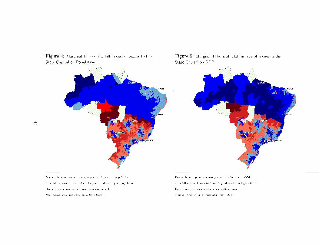
Figure 4: Marginal E�ects of a fall in cost of access to the
State Capital on Population
Deeper blues represent a stronger positive impact on population,
ie. a fall in travel costs to State Capital results in higher population.
Deeper reds represent a stronger negative impact.
Map constructed using estimates from table 4.
Figure 5: Marginal E�ects of a fall in cost of access to the
State Capital on GDP
Deeper blues represent a stronger positive impact on GDP,
ie. a fall in travel costs to State Capital results in higher GDP.
Deeper reds represent a stronger negative impact.
Map constructed using estimates from table 4.
44

Figure 6: Marginal E�ects (Population) on GDP di�erences
(South, North)-1
0-5
05
0 5 10Difference GDP AMC and endpoint
State Access Log Pop Margin Fitted values
-15
-10
-50
5
-5 0 5 10Difference GDP AMC and endpoint
State Access Log Pop Margin Fitted values
Marginal e�ects of a change in cost of access on population levels,
against the di�erence in GDP between AMC and endpoint.
Negative values occur when a fall in costs of access results in
higher population levels.
Figure 7: Marginal E�ects (Population) on Population dif-
ferences
-10
-50
5
-2 0 2 4 6 8Difference Population AMC and endpoint
State Access Log Pop Margin Fitted values
-15
-10
-50
5
-2 0 2 4 6 8Difference Population AMC and endpoint
State Access Log Pop Margin Fitted values
Marginal e�ects of a change in cost of access on population levels,
against the di�erence in population between AMC and endpoint.
Negative values occur when a fall in costs of access results in
higher population levels.
45

Supplementary Appendix
(not for publication)
The Model
Given output Yi = AiKαi L
1−αi , the pro�t maximization problem is t as:
maxK,L
p(1 − d)AiKαi L
1−αi − wc(1 − ηd)L− rc(1 − ρd)K,
where d is equal to 0 if i = c, and is strictly positive and between 0 and 1 otherwise.
The �rst order conditions are given by:
(1 − ηd)wc = p(1 − d)Ai(1 − α)
(Ki
Li
)α
Kβii ,
and
(1 − ρd)rc = p(1 − d)Aiα
(LiKi
)1−α
Kβii .
Expressing K as a function of L yields:
Ki
Li=
(1 − ηd)wc(1 − ρd)rc
α
1 − α. (1)
Reinserting this into the production function Yi = AiKαi L
1−αi , we get equation
(1).
It immediately follows that the derivative of the terms in bracket on the right
hand side of equation (2) with respect to d is given by:
∂ (1−ηd)wc
(1−ρd)rcα
1−α
∂d=
ρ− η
(1 − ρd)2wcrc
α
1 − α,
from which proposition 1 results.
1

Data
GDP Data
Andrade et al. (2004) describe the way IPEA estimates the municipality-level
GDP data. The �rst step involves calculating a municipality-level proxy for the
value added in agriculture, industry, and services respectively. For agriculture, it
combines gross total production and total expenditures in the local agricultural
sector from the Municipal Agricultural Census to generate a proxy for the value
added by agriculture in each municipality, and similarly for the valued added in
industry and services. This is then aggregated at the State level for every sector.
Finally, the municipality-level shares in the State level value added in each sector
are determined, and multiplied by the States' sector GDP as provided by IBGE.
The result is a set of estimates of municipality sector-level GDP, which sum to
equal total GDP.
Cost of Access Data
Castro �rst identi�ed main tra�c nodes across Brazil. For each of these nodes
and each of the three dates concerned, he identi�ed the shortest route to the
State Capital and São Paulo, with the connecting roads, and their quality. The
distances between each node were then calculated, with unpaved roads weighted
at 1.5 times that of paved roads due to the increased time of travel, and waterways
weighted at 10 times the cost of paved roads. If multiple routes lay within one
municipality, Castro took the average of the travel costs from these nodes as the
cost of access measure. If the municipality contained no nodes, he took the travel
cost from the node of a neighboring municipality, adding the expected distance
from this node weighted by 2 to represent the likely poor quality of any connection.
2

Reduced Form
Alternatively to model 3 in the main text, one can estimate the reduced form
model in di�erences:
∆Yis = α0 + α1Dis +X ′isα2 + θs + εis, (2)
where ∆Yis is the change in the outcome of interest in MCA i and State s
over the period of interest (alternatively 1970-2000, and sub-periods 1970-1980 or
1980-2000), estimated again as a function of distance to the lines Dis and a set
of controls for MCAs' initial conditions and �xed characteristics Xis, as well as
State �xed e�ects.
Results for this speci�cation are in Table A2. Over the period 1970-2000,
municipalities closer to the lines experienced increases in population, GDP and
GDP per capita relative to their more distant counterparts (column 1). The
respective elasticities are 0.068, 0.064, and 0.031 respectively and are statistically
signi�cant at the 1% level. When an interaction between distance and a Northern
dummy is included, the e�ects are similar, and stronger in the Southern part of
the country, with elasticities of 0.082, 0.096, and 0.044 for population, GDP and
GDP per capita respectively, compared to values of 0.043, 0.09, and 0.035 for the
North.1
All these results hold for the two sub-periods 1970-80, and 1980-2000, although
for GDP per capita, the e�ect is only signi�cant in the South, and in the second
sub-period. In terms of magnitude, e�ects on population are stronger in the �rst
sub-period, while for GDP they are stronger in the second one.
Benchmarking the magnitude of these e�ects as above, we �nd similar orders
of magnitude, with di�erences stemming from the distance to the line representing
one third of the change over the 1970-2000 period, while for GDP and GDP per
capita, the same ratio is only 7.6% and 7.3%.
1An F test fails to reject that the combined e�ects in the North are equal to zero for bothGDP and GDP per capita. The Northern Population e�ect is signi�cant.
3

Additional Results
Population Shares
Table A4 in the appendix, Panels A and B, provide further details on the evolution
of population, by looking at the changes in urban/rural and male/female shares
across the country's MCAs.
We focus on the speci�cation including the North dummy interactions. In
Panel A, the impact of a reduction of access costs to the state capitals on urban-
rural shares appears to be insigni�cant. In Panel B, Southern locations with
e�ective distance less than 90km have higher female shares. These thresholds are
close to the one found above for population. This is consistent with international
evidence showing that women, especially those in younger age group, move to
urban centers in greater numbers than men, driven by both work and marriage
prospects (e.g., Edlund, 2000).
Sectors of Production
We investigate speci�c areas of production to see if they can help explain these
results. In Table A4, panel C, we run estimations for the (log) GDP of agriculture,
industry, and services. Improved access to State capitals leads again to the dual
pattern found in Section 6. Industry and service GDP increase in the South
around the urban centers and the e�ect is reversed as e�ective distance grows.
The respective thresholds are 300km for services and 4650km for industry. In the
North, a reversed pattern again holds close to State capitals, where both industry
and service GDP decrease, while they start growing when distance exceeds 100
and 20km respectively.
Moreover, it is possible that di�erences in growth rates led to changes in the
relative importance of each sector, qualitatively altering the mix of local produc-
tion. To investigate this, panel D, shows a similar set of estimations where the
dependent variables are now sector shares in total GDP. The results indicate a
relative decrease of the share of industry around main urban centers in the South
(up to 230km) compensated to some extent by an increase in agriculture and
4

services.
Robustness Checks
First, in Table A5, we include a time interaction term on initial municipality levels
of water, electricity and toilet access. This controls for trends in improvements in
other infrastructure services. Municipalities nearer the straight lines may bene�t
from more investment in these other infrastructure services, for example electricity
networks may be focused along the routes connecting main urban centers. Alter-
natively the lines may not a�ect provision of these services, with municipalities
investing equally across space. Controlling for an overall trend in infrastructure
improvements means that the coe�cients on cost of access are purged from the
e�ect of localized improvements in other services that are due to being nearer or
further from these transport corridors, reinforcing our conditional excludability
condition.
Panel A gives the Population results, in which we see that the sign of the
e�ect remains the same, although the size is slightly reduced. This suggests that
other infrastructure services are acting against this pull on population; improved
services do not appear to be focused on the transport corridors, and hence may
keep people from moving towards them. Similarly in the North, we �nd the results
keep the same sign as in the standard regression in Table 4, however the size of the
results is slightly smaller. The e�ect of a reduction in transport cost is reduced
by local variations in improvements in other infrastructure services.
The same pattern is observed in the GDP results in panel B. The impact on
GDP per capita in panel C shows the reverse e�ect to those seen in Table 4.
However, as before, the e�ects are small and insigni�cant. This further suggests
that the impact of reductions in cost of access on GDP per capita is ambiguous,
and that the population and GDP e�ects cancel each other out on average.
As can be seen visually in Figures 4 and 5, municipalities in Brazil vary sub-
stantially in their area. To ensure our results are not biased by this size asymme-
try, Table A6 shows weighted estimations, in which we weight the municipality-
level observations by 1/area. In the South, the results are similar to those in Table
5
4, although the sizes of the e�ects are again slightly reduced. In the North, the
GDP results remain similar to the standard regression in Table 4, while the pop-
ulation e�ects are reduced, with the direct e�ect of cost of access on population
no longer being signi�cant (the coe�cient on squared cost of access is now only
signi�cant at 5%). The net e�ect of a reduction in the cost of access on population
is now consistent with the Southern results, with population increasing around
urban centers.
This is not surprising, as it is in the North where the majority of larger munic-
ipalities are located, so the weighted regression has a greater e�ect on this part of
the data. This may be partly explained if the emerging secondary cities discussed
in Section 6.1 are located in the larger municipalities observed in the North, and
therefore their in�uence is reduced in the weighted regression, hiding their impact
from our results. In consequence, we see GDP per capita being marginally af-
fected in the North (at the 10% level), and locations near state capitals see a fall
in their GDP per capita, as those locations further away gain from a reduction
in transport costs; secondary centers of output are being formed, but population
relocation to these areas does not entirely compensate for this.
Cost of Access to São Paulo
Table A7 shows the �rst-stage results when using the cost of access to São Paulo
as the R variable in (6) and (7). The F-statistic for the joint signi�cance of the
excluded instruments is 19.3, and 14.5 when a Northern dummy interaction is
added.
In terms of e�ects, locations bene�ted more from both state and municipal
roads the closer they are to the lines, while the reverse hold for federal paved
roads. However, as we would expect, interactions with a North dummy are not
signi�cant in this case. The closest Northern MCAs are more than 1,200 e�ective
kilometers away from São Paulo.
Second stage results are in Table A8, with panel A corresponding to popula-
tion, panel B to GDP, and panel C to GDP per capita. The OLS estimates in
columns 1, 4 and 7 show outcomes very similar to those using the cost of access to
6

the State capitals discussed in the main text. Both Population and GDP increased
in areas close enough to São Paulo, and this e�ect was reversed for locations far-
ther away. The results are con�rmed by the 2SLS estimates in columns 2, 5 and
8, with larger values of the coe�cients, and thresholds of 330km for population
and 400km for GDP respectively.
For GDP per capita, the OLS results are signi�cant and display again a non-
linear impacts of a fall in travel costs, with locations close to São Paulo experi-
encing a decrease, and locations farther away an increase. The 2SLS estimates in
column 8 are insigni�cant.
Finally, when adding an interaction with a dummy equal to 1 for Northern
MCAs, the results for the South hold, but we fail to �nd the dual pattern uncov-
ered for the cost of access to the State capitals. The fact that our instruments
do not perform very well for Northern interactions, and that the point estimates
for the South are largely unchanged in columns 3, 6 and 9 leads us to lend little
credit to the North results.
7

Appendix Tables and Figures
Table 1: A1 First Stage Pooled Cross SectionLog Cost of Access to State Capital Log Cost of Access to State Capital
VARIABLES with North dummy(1) (2)
Log Distance from Lines 0.0745*** 0.1104***(0.0124) (0.0150)
Northern * Distance -0.1024***(0.0244)
Constant 5.6265*** 6.1491***(0.2879) (0.3115)
Observations 3,638 3,638R2 0.6503 0.6524Chi2 all instruments signi�cant 36.00 53.99Prob. 0 0
Table A1 reports the �rst stage of the two-stage least square estimations reported in Table 3. It estimates cost of access tothe state capital in municipality i and State s in 2000 as a function of distance to the lines. Controls include state dummies,as well as the municipalities distance to Brasília, Sao Paulo and the state capital, dummies for whether the Amazon intersectswith the municipality, and whether the municipality is near the coast, and the municipalities area, and water, toilet and lightaccess. The geographical unit used is IPEA's 1970 Minimal Comparable Areas (AMC 70-00), which covers 3,599 municipalareas, comparable at any point between 1970 and 2000. Standard errors clustered at the municipality level are in parentheses.Stars indicate statistical signi�cance at the 1% (***), 5% (**), and 10% (*) level respectively.
8

Table 2: A2 Reduced FormA B C
Log Population Log GDP Log GDP/cap
YEAR VARIABLES (1) (2) (3) (4) (5) (6)
1970-2000
Log Distance from Lines -0.0684*** -0.0823*** -0.0640*** -0.0961*** -0.0309*** -0.0435***(0.0102) (0.0124) (0.0159) (0.0192) (0.0099) (0.0120)
Northern * Distance 0.0391** 0.0903*** 0.0354*(0.0199) (0.0308) (0.0191)
Log Population 1970 0.0286*** 0.0285***(0.0086) (0.0086)
Log GDP 1970 -0.1400*** -0.1398***(0.0109) (0.0109)
Log GDP per capita 1970 -0.6862*** -0.6857***(0.0142) (0.0142)
R2 0.3688 0.3695 0.1920 0.1939 0.5172 0.5177
1970-1980
Log Distance from Lines -0.0447*** -0.0545*** -0.0240* -0.0370*** -0.0052 -0.0005(0.0057) (0.0063) (0.0127) (0.0142) (0.0101) (0.0113)
Northern * Distance 0.0306*** 0.0404** -0.0149(0.0090) (0.0201) (0.0159)
Log Population 1970 0.0361*** 0.0363***(0.0048) (0.0048)
Log GDP 1970 -0.0791*** -0.0784***(0.0088) (0.0088)
Log GDP per capita 1970 -0.5193*** -0.5201***(0.0145) (0.0145)
R2 0.3008 0.3030 0.1105 0.1115 0.3640 0.3641
1980-2000
Log Distance from Lines -0.0288*** -0.0363*** -0.0499*** -0.0678*** -0.0349*** -0.0417***(0.0064) (0.0077) (0.0126) (0.0153) (0.0090) (0.0109)
Northern * Distance 0.0213* 0.0505** 0.0191(0.0124) (0.0246) (0.0175)
Log Population 1980 0.0303*** 0.0302***(0.0050) (0.0050)
Log GDP 1980 -0.1038*** -0.1040***(0.0084) (0.0084)
Log GDP per capita 1980 -0.5860*** -0.5859***(0.0138) (0.0138)
R2 0.3273 0.3279 0.2057 0.2066 0.4677 0.4679Observations 3,644 3,644 3,644 3,644 3,644 3,644
Table A2 reports reduced form estimations of changes in population (col. 1 & 2), GDP (col. 3 & 4) and GDP per capita (col. 5 & 6)in municipality i and State s in 2000, estimated as a function of distance to the lines and a set of controls including state dummies,as well as the municipality distance to Brasília, Sao Paulo and the state capital, dummies for whether the Amazon intersects with themunicipality, and whether the municipality is near the coast, and the municipality's area, and water, toilet and light access. The upperpanel reports estimates of the 1970-2000 change in outcomes, the intermediate panel reports estimates of the 1970-1980 changes, andthe lower panel reports estimates of the 1980-2000 changes. Standard errors clustered at the municipality level are in parentheses. Thegeographical unit used is IPEA's 1970 Minimal Comparable Areas (AMC 70-00), which covers 3,599 municipal areas, comparable atany point between 1970 and 2000. Stars indicate statistical signi�cance at the 1% (***), 5% (**), and 10% (*) level respectively.
9

Table 3: A3 First Stage of full 2SLSLog State Capital Travel Cost Log State Capital Travel Cost
VARIABLES with North dummy
km of federal paved roads/area*distance -46.8946*** -21.0440**(12.8050) (9.2735)
km of state roads/area*distance -2.5107 21.3469***(11.4583) (6.2040)
km of municipal roads/area*distance -0.2526 -2.6789***(1.4814) (0.9479)
Northern * km of federal paved roads/area*distance -7.4216(61.8975)
Northern * km of state roads/area*distance -65.2038**(25.5943)
Northern * km of municipal roads/area*distance 10.6998***(1.7669)
Observations 10,914 10,914R2 0.2018 0.2091Number of _ID 3,638 3,638F Test all instruments signi�cant 12.78 12.86All prob>F 0 0
Table A3 reports the �rst stage of the two-stage least square estimations reported in Table 4. It estimates cost of access to the statecapital in municipality i and State s and time t as a function of distance to the lines interacted with measures of the stocks in kilometersof federal, state, and municipal roads per squared-kilometers in State s at time t. Controls include municipality �xed e�ects, state-yeardummies, as well as the municipalities average water, toilet and light access in each period t. The geographical unit used is IPEA's 1970Minimal Comparable Areas (AMC 70-00), which covers 3,599 municipal areas, comparable at any point between 1970 and 2000. Standarderrors double-clustered at the municipality and state-year level are in parentheses. Stars indicate statistical signi�cance at the 1% (***),5% (**), and 10% (*) level respectively.
10

Table 4: A4 Two Stage Least Squares: Population and GDP sharesA B
Urban Population Share Female Population Share
(1) (2) (3) (4) (5) (6)VARIABLES OLS 2SLS 2SLS OLS 2SLS 2SLS
Log Cost of Access to State Capital 0.1144 0.1188 0.0921 -0.0149*** -0.0403* -0.0427(0.0697) (0.2485) (0.2603) (0.0050) (0.0224) (0.0264)
Squared Log Cost of Access to State Capital -0.0106* -0.0165 -0.0145 0.0016*** 0.0042** 0.0047**(0.0061) (0.0190) (0.0203) (0.0005) (0.0017) (0.0018)
Northern * Log Cost of Access to State Capital -0.4194 0.0315(0.5218) (0.0603)
Northern * Squared Log Cost of Access to State Capital 0.0370 -0.0034(0.0400) (0.0046)
Observations 10,914 10,914 10,914 10,914 10,914 10,914R2 0.8458 0.2873Number of _ID 3,638 3,638 3,638 3,638 3,638 3,638
C DLog GDP agriculture Log GDP industry Log GDP services Prop. agriculture Prop. industry Prop. services
(7) (8) (9) (10) (11) (12)VARIABLES 2SLS 2SLS 2SLS 2SLS 2SLS 2SLS
Log Cost of Access to State Capital -0.5529 -2.3078 -6.5013*** -0.5945 0.7936 -0.0254(1.7931) (1.4019) (0.8188) (0.6728) (0.5450) (0.3883)
Squared Log Cost of Access to State Capital 0.0333 0.1370 0.5604*** 0.0436 -0.0749 0.0144(0.1148) (0.1107) (0.0556) (0.0530) (0.0485) (0.0223)
Northern * Log Cost of Access to State Capital 2.8666 7.9175** 7.6178*** 0.3733 -0.3147 -0.5168(3.9704) (3.2388) (1.9455) (1.0428) (0.7131) (0.9916)
Northern * Squared Log Cost of Access to State Capital -0.2532 -0.7312*** -0.7301*** -0.0220 0.0279 0.0269(0.2996) (0.2474) (0.1442) (0.0795) (0.0563) (0.0725)
Observations 10,901 10,908 10,914 10,914 10,914 10,914R2 0.4642 0.5807Number of _ID 3,635 3,638 3,638 3,638 3,638 3,638
Table A4 reports the second stage of two-stage least square estimations of urban population shares (panel A, col. 1 to 3), female population shares (panel B, col. 4 to 6), log sector
GDP (panel C, col. 7 to 9), and sector GDP shares (panel D, col. 10 to 12) in municipality i, State s, and time t, estimated as a function of cost of access to the state capital and
cost of access squared, using the command xtivreg2 (Scha�er, 2010). The Cost of access variables are instrumented using distance to the lines, interacted with measures of the stocks in
kilometers of federal, state, and municipal roads per squared-kilometers in State s at time t (see �rst stage in A3). Controls include municipality �xed e�ects, state-year dummies, as well
as the municipalities' average water, toilet and light access in each period t, partialled out for the estimation of the standard errors. The geographical unit used is IPEA's 1970 Minimal
Comparable Areas (AMC 70-00), which covers 3,599 municipal areas, comparable at any point between 1970 and 2000. Standard errors double-clustered at the municipality and state-year
level are in parentheses. Stars indicate statistical signi�cance at the 1% (***), 5% (**), and 10% (*) level respectively.
11

Table 5: A5 Robustness: Time Interaction on Initial Water, Electricity and ToiletAccess
A B CLog Population Log GDP Log GDP/cap
VARIABLES (1) (2) (1) (2) (1) (2)
Log Cost of Access to State Capital -4.8604*** -4.7769*** -4.7427*** -5.6393*** 0.1177 -0.8623(0.9471) (0.8248) (1.2997) (1.1136) (0.9146) (0.8005)
Squared Log Cost of Access to State Capital 0.4288*** 0.4347*** 0.4006*** 0.4586*** -0.0282 0.0239(0.0628) (0.0641) (0.0795) (0.0791) (0.0514) (0.0431)
Northern * Log Cost of Access to State Capital 6.9796*** 8.4809*** 1.5013(1.4238) (2.0525) (2.0098)
Northern * Squared Log Cost of Access to State Capital -0.6509*** -0.7481*** -0.0972(0.1079) (0.1558) (0.1502)
Observations 10,914 10,914 10,914 10,914 10,914 10,914Number of _ID 3,638 3,638 3,638 3,638 3,638 3,638
Table A5 reports the second stage of two-stage least square estimations of log population (panel A, col. 1 & 2), log GDP (panel B,
col. 1 & 2) and log GDP per capita (panel C, col. 1 & 2) in municipality i, State s, and time t, estimated as a function of cost of
access to the state capital and cost of access squared, using the command xtivreg2 (Scha�er, 2010). The Cost of access variables are
instrumented using distance to the lines, interacted with measures of the stocks in kilometers of federal, state, and municipal roads per
squared-kilometers in State s at time t (see �rst stage in the Appendix). Controls include municipality �xed e�ects, state-year dummies,
municipalities' average water, toilet and light access in each period t, and a time interaction with initial municipality levels of water,
electricity and toilet access, partialled out for the estimation of the standard errors. The geographical unit used is IPEA's 1970 Minimal
Comparable Areas (AMC 70-00), which covers 3,599 municipal areas, comparable at any point between 1970 and 2000. Standard errors
double-clustered at the municipality and state-year level are in parentheses. Stars indicate statistical signi�cance at the 1% (***), 5%
(**), and 10% (*) level respectively.
Table 6: A6 Robustness: Weighted Regresion (1/Area)A B C
Log Population Log GDP Log GDP/cap
VARIABLES (1) (2) (3) (4) (5) (6)
Log Cost of Access to State Capital -3.5263*** -3.5599** -3.2195*** -3.3994** 0.3068 0.1605(1.1042) (1.4858) (1.1667) (1.3880) (0.8569) (0.9084)
Squared Log Cost of Access to State Capital 0.4173*** 0.4153*** 0.3695*** 0.3779*** -0.0478 -0.0374(0.0750) (0.0893) (0.0746) (0.0845) (0.0561) (0.0550)
Northern * Log Cost of Access to State Capital 0.6322 4.0385 3.4063(2.4914) (2.5135) (2.1723)
Northern * Squared Log Cost of Access to State Capital -0.1513 -0.4776** -0.3263*(0.1901) (0.2051) (0.1807)
Observations 10,914 10,914 10,914 10,914 10,914 10,914Number of _ID 3,638 3,638 3,638 3,638 3,638 3,638
Table A6 reports the second stage of weighted two-stage least square estimations of log population (panel A, col. 1 & 2), log GDP
(panel B, col. 1 & 2) and log GDP per capita (panel C, col. 1 & 2) in municipality i, State s, and time t, estimated as a function of cost
of access to the state capital and cost of access squared, using the command xtivreg2 (Scha�er, 2010). The weights are the inverse of
municipalities' area. The Cost of access variables are instrumented using distance to the lines, interacted with measures of the stocks in
kilometers of federal, state, and municipal roads per squared-kilometers in State s at time t (see �rst stage in the Appendix). Controls
include municipality �xed e�ects, state-year dummies, municipalities' average water, toilet and light access in each period t, and a time
interaction with initial municipality levels of water, electricity and toilet access, partialled out for the estimation of the standard errors.
The geographical unit used is IPEA's 1970 Minimal Comparable Areas (AMC 70-00), which covers 3,599 municipal areas, comparable
at any point between 1970 and 2000. Standard errors double-clustered at the municipality and state-year level are in parentheses. Stars
indicate statistical signi�cance at the 1% (***), 5% (**), and 10% (*) level respectively.
12

Table 7: A7 First Stage using Access to São PauloVARIABLES Log São Paulo Travel Cost São Paulo Travel Cost
(1) (2)
km of federal paved roads/area*distance -56.3802*** -62.6948***(7.5875) (8.3983)
km of state roads/area*distance 10.6428** 5.1613(4.8665) (5.6349)
km of municipal roads/area*distance 1.3862 1.8183*(0.9539) (1.0712)
Northern * km of federal paved roads/area*distance 17.1886(49.3896)
Northern * km of state roads/area*distance 6.8115(19.6505)
Northern * km of municipal roads/area*distance -0.7331(1.3041)
Observations 10,932 10,932R2 0.3182 0.3197Number of _ID 3,644 3,644F Test all instruments signi�cant 19.27 14.49All prob>F 0 0
Table A7 reports the �rst stage of the two-stage least square estimations reported in Table A8. It estimates cost
of access to Sao Paulo in municipality i and State s and time t as a function of distance to the lines interacted with
measures of the stocks in kilometers of federal, state, and municipal roads per squared-kilometers in State s at time
t. Controls include municipality �xed e�ects, state-year dummies, as well as the municipalities average water, toilet
and light access in each period t. The geographical unit used is IPEA's 1970 Minimal Comparable Areas (AMC
70-00), which covers 3,599 municipal areas, comparable at any point between 1970 and 2000. Standard errors
double-clustered at the municipality and state-year level are in parentheses. Stars indicate statistical signi�cance
at the 1% (***), 5% (**), and 10% (*) level respectively.
13

Table 8: A8 2SLS using Access to São PauloA B C
Log Population Log GDP Log GDP/cap
(1) (2) (3) (4) (5) (6) (7) (8) (9)VARIABLES OLS 2SLS 2SLS OLS 2SLS 2SLS OLS 2SLS 2SLS
Log Cost of Access to Sao Paulo -2.3277*** -4.2883*** -3.7200*** -1.8743*** -3.5797** -3.4434** 0.4535 0.7086 0.2765(0.3707) (1.0610) (0.9160) (0.5587) (1.5634) (1.4571) (0.3685) (1.2152) (1.2140)
Squared Log Cost of Access to Sao Paulo 0.2004*** 0.3591*** 0.3315*** 0.1438*** 0.2996*** 0.2948*** -0.0567* -0.0595 -0.0367(0.0353) (0.0644) (0.0590) (0.0517) (0.0887) (0.0837) (0.0302) (0.0679) (0.0670)
Northern * Log Cost of Access to Sao Paulo -43.4159 -37.0074 6.4085(27.8610) (60.9103) (38.3601)
Northern * Squared Log Cost of Access to Sao Paulo 2.6622 2.2722 -0.3900(1.7421) (3.8178) (2.4064)
Observations 10,932 10,932 10,932 10,932 10,932 10,932 10,932 10,932 10,932R2 0.4362 0.7364 0.7260Number of _ID 3,644 3,644 3,644 3,644 3,644 3,644 3,644 3,644 3,644
Table A8 reports the second stage of two-stage least square estimations of log population (col. 1 to 3), log GDP (col. 4 to 6) and log GDP per capita (col. 7 to 9)
in municipality i, State s, and time t, estimated as a function of cost of access to Sao Paulo and cost of access squared, using the command xtivreg2 (Scha�er, 2010).
The Cost of access variables are instrumented using distance to the lines, interacted with measures of the stocks in kilometers of federal, state, and municipal roads per
squared-kilometers in State s at time t (see �rst stage in the Table A7). Controls include municipality �xed e�ects, state-year dummies, as well as the municipalities' average
water, toilet and light access in each period t, partialled out for the estimation of the standard errors. The geographical unit used is IPEA's 1970 Minimal Comparable Areas
(AMC 70-00), which covers 3,599 municipal areas, comparable at any point between 1970 and 2000. Standard errors double-clustered at the municipality and state-year
level are in parentheses. Stars indicate statistical signi�cance at the 1% (***), 5% (**), and 10% (*) level respectively.
14

Figure 1: A1: Marginal E�ects of a fall in cost of access
to the State Capital on GDP, using interaction on endpoint
initial GDP
Deeper blues represent a stronger positive impact on GDP,
ie. a fall in travel costs to State Capital results in higher GDP.
Deeper reds represent a stronger negative impact.
Map constructed using estimates from Table 4.
Figure 2: A2: Marginal E�ects of a fall in cost of access
to the State Capital on GDP, using interaction on endpoint
initial water access proportions
Deeper blues represent a stronger positive impact on GDP,
ie. a fall in travel costs to State Capital results in higher GDP.
Deeper reds represent a stronger negative impact.
Map constructed using estimates from Table 4.
15

Figure 3: A3: Marginal E�ects of a fall in cost of access
to the State Capital on GDP, using interaction on endpoint
initial schooling levels
Deeper blues represent a stronger positive impact on GDP,
ie. a fall in travel costs to State Capital results in higher GDP.
Deeper reds represent a stronger negative impact.
Map constructed using estimates from Table 4.
Figure 4: A4: Marginal E�ects of a fall in cost of access
to the State Capital on GDP, using interaction on endpoint
initial manufacturing to services ratio
Deeper blues represent a stronger positive impact on GDP,
ie. a fall in travel costs to State Capital results in higher GDP.
Deeper reds represent a stronger negative impact.
Map constructed using estimates from Table 4.
16

Figure 5: A5 Marginal E�ects (GDP) on GDP di�erences
(South, North)-1
0-5
05
0 5 10Difference GDP AMC and endpoint
State Access Log GDP Margin Fitted values
-20
-15
-10
-50
5
-5 0 5 10Difference GDP AMC and endpoint
State Access Log GDP Margin Fitted values
Marginal e�ects of a change in cost of access on GDP,
against the di�erence in GDP between AMC and endpoint.
Negative values occur when a fall in costs of access results in
higher population levels.
Figure 6: Marginal E�ects (GDP) on Population di�erences
-10
-50
5
-2 0 2 4 6 8Difference Population AMC and endpoint
State Access Log GDP Margin Fitted values
-20
-15
-10
-50
5
-2 0 2 4 6 8Difference Population AMC and endpoint
State Access Log GDP Margin Fitted values
Marginal e�ects of a change in cost of access on GDP,
against the di�erence in population between AMC and endpoint.
Negative values occur when a fall in costs of access results in
higher population levels.
17

Figure 7: State level GDP per capita impacts of road
improvements, as ratio of actual GDP per capita growth
1970-2000
Impact on fall in costs of access on GDP/cap as a ratio of actual change
calculated using marginal e�ects derived from Table 4
Deeper blues represent higher proportion of GDP/cap explained by road
improvements.
Reds represent states where GDP per capita was reduced by road placement.
18

Appendix References
Andrade, E., Laurini, M., Madalozzo, R., and P.L. Valls Pereira. 2004, �Conver-
gence clubs among Brazilian municipalities�. Economics Letters, 83, 179�184.
Edlund, L., 2000, �On the Geography of Demography: Why Women Live
in Cities,�Econometric Society World Congress 2000 Contributed Papers 1147,
Econometric Society.
19