the binary stars 1918
TRANSCRIPT

8/2/2019 The Binary Stars 1918
http://slidepdf.com/reader/full/the-binary-stars-1918 1/349
8/2/2019 The Binary Stars 1918
http://slidepdf.com/reader/full/the-binary-stars-1918 2/349

8/2/2019 The Binary Stars 1918
http://slidepdf.com/reader/full/the-binary-stars-1918 3/349

8/2/2019 The Binary Stars 1918
http://slidepdf.com/reader/full/the-binary-stars-1918 4/349
Digitized by the Internet Archive
in 2007 with funding from
IVIicrosoft Corporation

8/2/2019 The Binary Stars 1918
http://slidepdf.com/reader/full/the-binary-stars-1918 5/349

8/2/2019 The Binary Stars 1918
http://slidepdf.com/reader/full/the-binary-stars-1918 6/349

8/2/2019 The Binary Stars 1918
http://slidepdf.com/reader/full/the-binary-stars-1918 7/349
THE BINARY STARS

8/2/2019 The Binary Stars 1918
http://slidepdf.com/reader/full/the-binary-stars-1918 8/349

8/2/2019 The Binary Stars 1918
http://slidepdf.com/reader/full/the-binary-stars-1918 9/349

8/2/2019 The Binary Stars 1918
http://slidepdf.com/reader/full/the-binary-stars-1918 10/349
umaammmmam
Plate I. The Thirty-Six-Inch Retractor of the Lick Observatory
8/2/2019 The Binary Stars 1918
http://slidepdf.com/reader/full/the-binary-stars-1918 11/349
THE BINARY STARS
BT ROBERT GRANT AITKEN
Astronomer in the Lick Observatory
University of California
\
NEW YORK
1918

8/2/2019 The Binary Stars 1918
http://slidepdf.com/reader/full/the-binary-stars-1918 12/349
Copyrighty igiSy by Douglas C. McMurtrte
^3
^3

8/2/2019 The Binary Stars 1918
http://slidepdf.com/reader/full/the-binary-stars-1918 13/349
TO
Sherburne Wesley Burnham
THIS volume
IS GRATEFULLY INSCRIBED

8/2/2019 The Binary Stars 1918
http://slidepdf.com/reader/full/the-binary-stars-1918 14/349

8/2/2019 The Binary Stars 1918
http://slidepdf.com/reader/full/the-binary-stars-1918 15/349
PREFACE
Credit has been given on many pages of this volume for
assistance received in the course of its preparation; but I
desire to express in this more formal manner my special grati-
tude, first of all, to my colleague. Dr. J. H. Moore, for con-
tributing the valuable chapter on The Radial Velocity of a
Star; also to Director E. C. Pickering and Miss Annie J.
Cannon, of the Harvard College Observatory, for generously
permitting me to utilize data from the New Draper Catalogue
of Stellar Spectra; to Professor H. N. Russell, of Princeton
University, Professor F. R. Moulton, of the University of
Chicago, Professor E. E. Barnard, of the Yerkes Observatory,
and Dr. H. D. Curtis, my colleague, for putting at my disposal
published and unpublished material; and, finally, to Director
W. W. Campbell, for his constant interest in and encourage-
ment of my work. Nearly all of the manuscript has been read
by Dr. Campbell and by Dr. Curtis, and several of the chapters
also by Dr. Moore and by Dr. Reynold K. Young, and I am
deeply indebted to them for their friendly criticism.
The book appears at this particular time in order that it
may be included in the series of Semi-Centennial Publications
issued by the University of California.
R. G. AlTKEN
December, igiy

8/2/2019 The Binary Stars 1918
http://slidepdf.com/reader/full/the-binary-stars-1918 16/349

8/2/2019 The Binary Stars 1918
http://slidepdf.com/reader/full/the-binary-stars-1918 17/349
CONTENTS
Page
Introduction xiii
Chapter I. Historical Sketch: The Early Period . . i
Chapter II. Historical Sketch: The Modern Period 21
Chapter III. Observing Methods, Visual Binary Stars 40
Chapter IV. The Orbit of a Visual Binary Star . . 65
Chapter V. The Radial Velocity of a Star, by Dr.
J. H. Moore . 107
Chapter VI. The Orbit of a Spectroscopic Binary Star 134
Chapter VII. Eclipsing Binary Stars 167
Chapter VIII. The Known Orbits of Visual and Spec-
troscopic Binary Stars 192
Chapter IX. Some Binary Systems of Special Interest 226
Chapter X. A Statistical Study of the Visual Double
Stars in the Northern Sky 252
Chapter XI. The Origin of the Binary Stars .... 274

8/2/2019 The Binary Stars 1918
http://slidepdf.com/reader/full/the-binary-stars-1918 18/349

8/2/2019 The Binary Stars 1918
http://slidepdf.com/reader/full/the-binary-stars-1918 19/349
ILLUSTRATIONS
Page
Plate I. The Thirty-Six-Inch Refractor of the Lick
Observatory Frontispiece
Plate II. The Micrometer for the Thirty-Six-Inch
Refractor 41
Plate III. Spectra of U4 Eridani, a Carinae, the Sun
and az Centauri 114
Plate IV. The Mills Spectrograph 117
Plate V. Photographs of Krueger 60, in igo8 and in
1915, by Barnard 230
Figure i. Diagram to Illustrate Variable Radial
Velocity 27
Figure 2. Diagram to Illustrate Transit Method of
Determining Micrometer-Screw Value . 44
Figure 3. The Apparent Orbit of A 88 84
Figure 4. The True and Apparent Orbits of a Double
Star {after See) 91
Figure 5. Apparent and True Orbits and Interpolating
Curve of Observed Distances for a Binary
System in which the Inclination is go° . 96
Figure 6. Rectilinear Motion 104
Figure 7. Diagram to Illustrate the Relations between
Orbital Motion and Radial Velocity in a
Spectroscopic Binary 135
Figure 8. Velocity Curve of k Velorum 141

8/2/2019 The Binary Stars 1918
http://slidepdf.com/reader/full/the-binary-stars-1918 20/349
Xll ILLUSTRATIONSPage
Figure 9. King's Orbit Method. Graph for e = o.ys,
0) = 60° 155
Figure 10. Radial Velocity Curve for f Geminorum^
Showing Secondary Oscillation .... 163
Figure ii. Light-Curve of the Principal Minimum of
W Delphini 181
Figure 12. The System of W Delphini 188

8/2/2019 The Binary Stars 1918
http://slidepdf.com/reader/full/the-binary-stars-1918 21/349
INTRODUCTION
It is the object of this volume to give a general account of
our present knowledge of the binary stars, including such an
exposition of the best observing methods and of approved
methods of orbit computation as may make it a useful guide
for those who wish to undertake the investigation of thesesystems; and to present some conclusions based upon the
author's own researches during the past twenty years.
The term binary star was first used by Sir William Herschel,
in 1802, in his paper "On the Construction of the Universe,"
to designate "a real double star—the union of two stars, that
are formed together in one system, by the laws of attraction."
The term double star is of earlier origin ; its Greek equivalent
was, in fact, used by Ptolemy to describe the appearance of v
Sagittarii, two fifth magnitude stars whose angular separation
is about 14', or a little less than half of the Moon's apparent
diameter. It is still occasionally applied to this and other
pairs of stars visible to the unaided eye, but is generally em-
ployed to designate pairs separated by only a few seconds of
arc and therefore visible as two stars only with the aid of a
telescope.
Not every double star is a binary system, for, since all of the
stars are apparently mere points of light projected upon the
surface of the celestial sphere, two unrelated stars may appear
to be closely associated simply as the result of the laws of
perspective. Herschel draws the distinction between the two
classes of objects in the following words:
". . . if a certain star should be situated at any, per-
haps immense, distance behind another, and but little deviating
from the line in which we see the first, we should have the
appearance of a double star. But these stars being totally
unconnected would not form a binary system. If, on the con-
trary, two stars should really be situated very near each other,
and at the same time so far insulated as not to be materially

8/2/2019 The Binary Stars 1918
http://slidepdf.com/reader/full/the-binary-stars-1918 22/349
xiv INTRODUCTION
affected by neighboring stars, they will then compose a sep-
arate system, and remain united by the bond of their mutual
gravitation toward each other. This should be called a real
double star."
Within the last thirty years we have become acquainted
with a class of binary systems which are not double stars in
the ordinary sense of the term at all, for the two component
stars are not separately visible in any telescope. These are
the spectroscopic binary stars, so named because their existence
is demonstrated by a slight periodic shifting to and fro of the
lines in their spectra, which, as will be shown, is evidence of a
periodic variation in the radial velocity (the velocity in the
line of sight, toward or away from the observer) of the star.
The only differences between the spectroscopic and the visual
binary ("real double") stars are those which depend upon the
degree of separation of the two components. The components
of a spectroscopic binary, are, in general, less widely sep-
arated than those of a visual binary, consequently they are
not separately visible even with the most powerful telescopes
and the systems have relatively short periods of revolution.
In the present volume the two classes will be regarded as
members of a single species.

8/2/2019 The Binary Stars 1918
http://slidepdf.com/reader/full/the-binary-stars-1918 23/349
CHAPTER I
HISTORICAL SKETCH: THE EARLY PERIOD
The first double star was discovered about the year 1650
by the Italian astronomer, Jean Baptiste Riccioli. This was
f Ursae Majoris (Mizar). Itis
a remarkable coincidence thatMizar was also the first double star to be observed photographi-
cally, measurable images being secured by G. P. Bond, at the
Harvard College Observatory in 1857; and that its principal
component was the first spectroscopic binary to be discovered,
the announcement being made by E. C. Pickering in 1889.
In 1656, Huyghens saw Ononis resolved into the three
principal stars of the group which form the familiar Trape-
zium, and, in 1664, Hooke noted that 7 Arietis consisted of
two stars. At least two additional pairs, one of which proved
to be of more than ordinary interest to astronomers, were dis-
covered before the close of the Seventeenth Century. It is
worthy of passing note that these were southern stars, not
visible from European latitudes,—a Cruets, discovered by the
Jesuit missionary, Father Fontenay, at the Cape of Good
Hope, in 1685, and a Centauri, discovered by his confrere,
Father Richaud, while observing a comet at Pondicherry,
India, in December, 1689.
These discoveries were all accidental, made in the course of
observations taken for other purposes. This is true also of the
double stars found in the first three-quarters of the Eighteenth
Century. Among these were the discoveries of 7 Virginis, in
1718, and of Castor, in 1719, by Bradley and Pound, and of
61 Cygni, by Bradley, in 1753.
No suspicion seems to have been entertained by these as-
tronomers or by their contemporaries that the juxtaposition
of the two star images in such pairs was other than optical,
due to the chance positions of the Earth and the two stars in
nearly a straight line. They were therefore regarded as mere

8/2/2019 The Binary Stars 1918
http://slidepdf.com/reader/full/the-binary-stars-1918 24/349
2 THE BINARY STARS
curiosities, and no effort was made to increase their number;
nor were observations of the relative positions of the two com-
ponents recorded except in descriptive terms. Father Feuille,
for instance, on July 4, 1709, noted that the fainter star in the
double, a Centauri, "is the more western and their distance is
equal to the diameter of this star," and Bradley and Pound
entered in their observing book, on March 30, 1719, that "the
direction of the double star a of Gemini was so nearly parallel
to a line through k and a of Gemini that, after many trials, we
could scarce determine onwhich
side of a the line from k par-
allel to the line of their direction tended; if on either, it was
towards /3."
Halley's discovery, in 1718, that some of the brighter stars,
Sirius, Arcturus, Aldebaran, were in motion, having unmis-
takably changed their positions in the sky since the time of
Ptolemy, unquestionably stimulated the interest of astron-
omers in precise observations of the stars. These researches
and their results, in turn, were probably largely responsible for
the philosophical speculations which began to appear shortly
after the middle of the Eighteenth Century as to the possi-
bility of the existence of systems among the stars. Famous
among the latter are the Cosmologische Briefe,^ published in
1 761 by Lambert, in which it is maintained that the stars are
suns and are accompanied by retinues of planets. Lambert,
however, apparently did not connect his speculations with the
double stars then known. Six years later, in 1767, John
Michell, in a paper read before the Royal Society of London,
presented a strong argument, based upon the theory of proba-
bilities, that "such double stars, etc., as appear to consist of
two or more stars placed near together, do really consist of
stars placed near together, and under the influence of some
general law, whenever the probability is very great, that there
would not have been any such stars so near together, if all
those that are not less bright than themselves had been scat-
tered at random through the whole heavens." Michell thus
has the credit of being the first to establish the probability of
1 Cosmologische Briefe iiber die Einrichtung des Weltbaues, Ausgefertigt von J. H. Lam-
bert, Augsburg, 1 76 1.

8/2/2019 The Binary Stars 1918
http://slidepdf.com/reader/full/the-binary-stars-1918 25/349
THE BINARY STARS 3
the existence of physical systems among the stars ; • but there
were no observational data to support his deductions and they
had no direct influence upon the progress of astronomy.
The real beginning of double star astronomy dates from the
activities of Christian Mayer and, in particular, of Sir William
Herschel, in the last quarter of the Eighteenth Century. If
a definite date is desired we may well follow Lewis in adopting
the year 1779, for that year is marked by the appearance of
Mayer's small book entitled "De novis in Coelo Sidereo Phae-
nominis in miris Stellarum fixarum Comitibus," wherein hespeculates upon the possibility of small suns revolving around
larger ones, and by the beginning of Herschel's systematic
search for double stars.
The difference between Mayer's speculations and earlier ones
is that his rest in some degree at least upon observations.
These were made with an eight-foot Bird mural quadrant at
Mannheim,in
1777 and 1778. At anyrate, in his
book justreferred to, he publishes a long list of faint companions ob-
served in the neighborhood of brighter stars.^ As one result
of his observations he sent to Bode, at Berlin, the first collec-
tion or catalogue of double stars ever published. The list
contained earlier discoveries as well as his own and is printed
in the Astronomisches Jahrbuch for the year 1784 (issued in
1 781) under the caption, "Verzeichnis aller bisher entdeckten
Doppelsterne." The following tabulation gives the first five
entries:
Gerade
Aufst.
Abwei-
chung
Unterschied
Abstand
Stellung
Grosse in der in derdes
Klei-Aufst. Abw.
nernG. M. G. M. Sec. Sec. Sec.
Andromeda beyde Qter 8 38 2945 N 45 24 46 S. W.
Andromeda beyde Qter 13 13 20 18 N 15 29 32 S. 0.
f Fische 6. und yter 15 33 625N 22 9 24 N. 0.
beyAt Fische beyde yter 19 24 5 oN 4 4 S.
7 Widder beyde 5ter 25 22 18 13 N 3 12 12 s. w.
* This list, rearranged according to constellations, was reprinted by Schjellerup in the
journal Copernicus, vol. 3, p. 57, 1884.

8/2/2019 The Binary Stars 1918
http://slidepdf.com/reader/full/the-binary-stars-1918 26/349
4 THE BINARY STARS
In all, there are eighty entries, many of which, like Castor
and 7 Virginis, are among the best known double stars. Others
are too wide to be found even in Herschel's catalogues and afew cannot be identified with certainty. Southern pairs, like
a Centauri, are of course not included, and curiously enough,
6 Ononis is not listed. The relative positions given for the
stars in each pair are little better than estimates, for precise
measures were not practicable until the invention of the
'revolving micrometer'.
In his comments on Mayer's catalogue Bode points out thatcareful observations of such pairs might become of special
value in the course of time for the discovery of proper motions,
since it would be possible to recognize the fact of motion in
one or the other star as soon as the distance between them had
changed by a very few seconds of arc. Mayer himself seems
to have had proper motions in view in making his observa-
tions and catalogue rather than any idea of orbital motions.
Sir William Herschel "began to look at the planets and the
stars" in May, 1773; on March i, 1774, "he commenced his
astronomical journal by noting that he had viewed Saturn's
ring with a power of forty, appearing 'like two slender arms'
and also 'the lucid spot in Orion's sword belt'." The earliest
double star measure recorded in his first catalogue is that of
6 Ononis, on November 11, 1776, and he made a few others
in the two years following. It was not until 1779, however,
that he set to work in earnest to search for these objects, for
it was then that he conceived the idea of utilizing them to test
a method of measuring stellar parallax suggested long before
by Galileo. The principle involved is very simple. If two
stars are in the same general direction from us and one is
comparatively near us while the other is extremely distant,
the annual revolution of the Earth about the Sun will produce
a periodic variation in the relative positions of the two. As a
first approximation, we may regard the more distant star as
absolutely fixed and derive the parallax of the nearer one
from the measured displacements.
It seemed clear to Herschel that the objects best fitted for
such an investigation were close double stars with components

8/2/2019 The Binary Stars 1918
http://slidepdf.com/reader/full/the-binary-stars-1918 27/349
THE BINARY STARS 5
of unequal brightness. He pointed out in his paper "On the
Parallaxes of the Fixed Stars", read before the Royal Society
in 1 78 1, that the displacement could be more easily and cer-
tainly detected in a close double star than in a pair of stars
more widely separated and also that in the former case the
observations would be free from many errors necessarily af-
fecting the measures in the latter.
"As soon as I was fully satisfied," he continues, "that in the
investigation of parallax the method of double stars would
have many advantages above any other, it became necessary
to look out for proper stars. This introduced a new series of
observations. I resolved to examine every star in the heavens
with the utmost attention and a very high power, that I
might collect such materials for this research as would enable
me to fix my observations upon those that would best answer
my ends."
In this reasoning, Herschel assumes that there is no physical
connection between the components of such close double stars,
—a fact upon which every writer on the history of double star
astronomy has commented. This was not an oversight on his
part, for at the close of his first catalogue of double stars he
remarks, "I preferred that expression {i.e., double stars) to any
other, such as Comes, Companion, or Satellite; because, in my
opinion, it is much too soon to form any theories about smallstars revolving round large ones, and I therefore thought it
advisable carefully to avoid any expression that might convey
that idea."
Herschel's telescopes were more powerful than any earlier
ones and with them he soon discovered a far larger number
of double stars than he had anticipated. With characteristic
thoroughness he nevertheless decided to carry out his plan of
examining "every star in the heavens," and carefully recorded
full details of all his observations. These included a general
description of each pair and also estimates, or measures with
the "revolving micrometer," or "lamp micrometer," both in-
vented by himself, of the apparent distance between the two
components and of the direction of the smaller star from the
larger. The direction, or position angle, of the smaller star,

8/2/2019 The Binary Stars 1918
http://slidepdf.com/reader/full/the-binary-stars-1918 28/349
6 THE BINARY STARS
by his definition, was the angle at the larger star between the
line joining the two stars and a line parallel to the celestial
equator. The angle was always made less than 90°, the letters,
w/, sf, sp, and np being added to designate the quadrant. His
first catalogue, presented to the Royal Society on January 10,
1782, contains 269 double stars, "227 of which, to my
present knowledge, have not been noticed by any person."
A second catalogue, containing 434 additional objects, was
presented to the same society in 1784. The stars in these
catalogues were divided into six classes according to angular
separation.
"In the first," he writes, "I have placed all those which
require indeed a very superior telescope, the utmost clearness
of air, and every other favorable circumstance to be seen at
all, or well enough to judge of them. ... In the second
class I have put all those that are proper for estimations by
the eye or very delicate measures of the micrometer..
In the third class I have placed all those . . . that
are more than five but less than 15" asunder; . . . The
fourth, fifth, and sixth classes contain double stars that are
from 15" to 30", from 30" to i' and from i' to 2' or more
asunder."
Class I, in the two catalogues, includes ninety-seven pairs,
and contains such systems as r Ophiuchi, 8 Herculis, e Bootis,
^ Ursae Majoris, 4 Aquarii, and f Cancri. In general, Herschel
did not attempt micrometer measures of the distances of these
pairs because the finest threads available for use in his micro-
meters subtended an angle of more than i". The following
extracts will show his method of estimating the distance in
such cases and of recording the position angle, and also the
care with which he described the appearance of each object.
The dates of discovery, or of the first observation, here
printed above the descriptions, are set in the margin at the
left in the original.
H. I. September 9, 1779
e Bootis, Flamst. 36. Ad dextrum femur in perizomate. Double. Very
unequal. L. reddish; 6". blue, or rather a faint lilac. A very beautiful object.
The vacancy or black division between them, with 227 is ^ diameter of

8/2/2019 The Binary Stars 1918
http://slidepdf.com/reader/full/the-binary-stars-1918 29/349
THE BINARY STARS 7
5.; with 460, I yi diameter of L.; with 932, near 2 diameters of L,; with
1,159, still farther; with 2,010 (extremely distinct), ^ diameters of L.
These quantities are a mean of two years' observation. Position 31" 34' n
preceding.
H. 2. May 2, 1780
i Ursae Majoris. Fl. 53. In dextro posteriore pede. Double. A little
unequal. Both w [white] and very bright. The interval with 222 is ^diameter of L.; with 227, i diameter of L; with 278, near \]/2 diameter of
L. Position 53° 47' s following.
Careful examination of the later history of the stars of
Herschel's Class I shows that the majority had at discovery
an angular separation of from 2" to 3.5"; a half dozen pairs
as wide as 5" are included (one with the ms. remark, "Too far
asunder for one of the first class"); and a number as close
as or closer than \", Seven of these stars do not appear
in the great catalogue of Struve, but five of these have been
recovered by later observers, leaving only two that cannot be
identified.
In passing judgment upon the accuracy, or the lack of it, in
Herschel's measures of double stars, it is necessary to hold in
mind the conditions under which he had to work. His reflec-
tors (all of his own construction) were indeed far more powerful
telescopes than any earlier ones, especially the "twenty-feet
reflector," with mirror of eighteen and three-quarter inchesaperture, and the great "forty-feet telescope," with its four-foot
mirror. But these telescopes were unprovided with clock-
work; in fact their mountings were of the alt-azimuth type.
It was therefore necessary to move the telescope continuously
in both coordinates to keep a star in the field of view and the
correcting motions had to be particularly delicate when high-
power eye-pieces, such as are necessary in the observation of
close double stars, were employed. Add the crude forms of
micrometers at his disposal, and it will appear that only an
observer of extraordinary skill would be able to make measures
of any value whatever.
No further catalogues of double stars were published by
Herschel until June 8, 1821, about a year before his death,
when he presented to the newly founded Royal Astronomical

8/2/2019 The Binary Stars 1918
http://slidepdf.com/reader/full/the-binary-stars-1918 30/349
8 THE BINARY STARS
Society a final list of 145 new pairs, not arranged in classes,
and, for the most part, without measures.
After completing his second catalogue, in 1784, Herschel
seems to have given relatively little attention to double stars
until about the close of the century and, though he doubtless
tested it fully, there is no mention of his parallax method in
his published writings after the first paper on the subject. Athorough review of his double star discoveries which he insti-
tuted about the year 1797 with careful measures, repeated in
some cases on many nights in different years, revealed aremarkable change in the relative positions of the com-
ponents in a number of double stars during the interval
of nearly twenty years since their discovery, but this
change was of such a character that it could not be produced
by parallax.
We have seen that, in 1782, Herschel considered the time
not ripe for theorizing as to the possible revolution of smallstars about larger ones. Probably no astronomer of his own
or of any other age was endowed in a higher degree than
Herschel with what has been termed the scientific imagination
certainly no one ever more boldly speculated upon the deepest
problems of sidereal astronomy ; but his speculations were the
very opposite of guesswork, invariably they were the results of
critical analyses of the data given by observation and were
tested by further observations when possible. Michell, in
1783, applied his earlier argument from the theory of probabili-
ties to the double stars in Herschel's first catalogue and con-
cluded that practically all of them were physical systems ; but
it was not until July, 1802, that Herschel himself gave any
intimation of holding similar views. On that date he presented
to the Royal Society a paper entitled "Catalogue of 500 new
Nebulae, nebulous Stars, planetary Nebulae, and Clusters of
Stars; with Remarks on the Construction of the Heavens", in
which he enumerates "the parts that enter into the construc-
tion of the heavens" under twelve heads, the second being,
"H. Of Binary sidereal Systems, or double Stars." In
this section he gives the distinction between optical and
binary systems quoted in my Introduction and argues as to

8/2/2019 The Binary Stars 1918
http://slidepdf.com/reader/full/the-binary-stars-1918 31/349
THE BINARY STARS 9
the possibility of systems of the latter type under the law of
gravitation.
On June 9, 1803, followed the great paper in which he gave
the actual demonstration, on the basis of his measures, that
certain double stars are true binary systems. This paper, the
fundamental document in the physical theory of double stars,
is entitled, "Account of the Changes that have happened,
during the last Twenty-five Years, in the relative Situation of
Double-stars; with an Investigation of the Cause to which
they are owing." After pointing out that the actual existence
of binary systems is not proved by the demonstration that
such systems may exist, Herschel continues, "I shall therefore
now proceed to give an account of a series of observations
on double stars, comprehending a period of about twenty-
five years which, if I am not mistaken, will go to prove,
that many of them are not merely double in appearance,
but must be allowed to be real binary combinations of twostars, intimately held together by the bonds of mutual
attraction."
Taking Castor as his first example, he shows that the change
in the position of the components is real and not due to any
error of observation. Then, by a masterly analysis of every
possible combination of motions of the Sun and the compo-
nentsin this,
andin five other systems,
heproves that orbital
motion is the simplest and most probable explanation in any
one case, and the only reasonable one when all six are considered.
His argument is convincing, his conclusion incontrovertible,
and his paper, a year later, containing a list of fifty additional
double stars, many of which had shown motion of a similar
character, simply emphasizes it.
This practically concluded Sir William Herschel's contribu-
tions to double star astronomy, for his list of 145 new pairs,
published in 1821, was based almost entirely upon observations
made before 1802. In fact, little was done in this field by any
one from 1804 until about 1 8 16. Sir John Herschel, in that
year, decided to review and extend his father's work and had
made some progress when Sir James South, who had indepen-
dently formed similar plans, suggested that they cooperate.

8/2/2019 The Binary Stars 1918
http://slidepdf.com/reader/full/the-binary-stars-1918 32/349
10 THE BINARY STARS
The suggestion was adopted and the result was a catalogue of
380 stars, based upon observations made in the years 1821 to
1823 with South's five-foot and seven-foot refractors, of 3^"and 5" aperture respectively. These telescopes were mounted
equatorially but were not provided with driving-clocks. They
were, however, equipped with micrometers in which the par-
allel threads were fine spider lines. The value of the catalogue
was greatly increased by the inclusion of all of Sir William
Herschel's measures, many of which had not before been
published.Both of these astronomers devoted much attention to double
stars in following years, working separately however. South
with his refractors, Herschel with a twenty-foot reflector
(eighteen-inch mirror) and later with the five-inch refractor
which he had purchased from South. They not only remea-
sured practically all of Sir William Herschel's double stars,
some of them onmany
nights in different years, but they, and
in particular Sir John Herschel, added a large number of new
pairs. Indeed, so numerous were J. Herschel's discoveries and
so faint were many of the stars that he deemed some apology
necessary. He says, ". . .so long as no presumption a
priori can be adduced why the most minute star in the heavens
should not give us that very information respecting parallax,
proper motion, and an infinity of other interesting points,
which we are in search of, and yet may never obtain from its
brighter rivals, the minuteness of an object is no reason for
neglecting its examination. . . . But if small double stars
are to be watched, it is first necessary that they should become
known ; nor need we fear that the list will become overwhelm-
ing. It will be curtailed at one end, by the rejection of un-
interesting and uninstructive objects, at least as fast as it is
increased on the other by new candidates." The prediction
made in the closing sentence has not been verified; on the
contrary, the tendency today is rather to include in the great
reference catalogues every star ever called double, even those
rejected later by their discoverers.
The long series of measures and of discoveries of double stars
by Herschel and South were of great value in themselves and

8/2/2019 The Binary Stars 1918
http://slidepdf.com/reader/full/the-binary-stars-1918 33/349
THE BINARY STARS II
perhaps of even greater value in the stimulus they gave to the
observation of these objects by astronomers generally, and well
merited the gold medals awarded to their authors by the Royal
Astronomical Society. The measures, however, are now as-
signed small weight on account of the relatively large errors of
observation due to the conditions under which they were of
necessity made; and of the thousands of new pairs very few
indeed have as yet proved of interest as binaries. The great
majority are too wide to give the slightest evidence of orbital
motion in the course of a century.
The true successor to Sir William Herschel, the man who
made the next real advance in double star astronomy, an
advance so great that it may indeed be said to introduce a new
period in its history, was F. G. W. Struve. Wilhelm Struve
became the director of the observatory at Dorpat, Russia, in
1 813, and soon afterwards began measuring the differences in
right ascension and in declination between the components of
double stars with his transit instrument, the only instrument
available. A little later he acquired a small equatorial, inferior
to South's, with which he continued his work, and, in 1822, he
published his "Catalogus 795 stellarum duplicium." This
volume is interesting but calls for no special comment because
Struve's great work did not really begin until two years later,
in
November, 1824, when he receivedthe celebrated Fraun-
hofer refractor.
This telescope as an instrument for precise measurements
was far superior to any previously constructed. The tube was
thirteen feet long, the objective had an aperture of nine Paris
inches,^ the mounting was equatorial and of very convenient
form, and, best of all, was equipped with an excellent driving
clock. So far as I am aware, this was the first telescope em-
ployed in actual research to be provided with clock-work
though Passement, in 1757, had "presented a telescope to the
King [of France], so accurately driven by clock-work that it
would follow a star all night long." A finder of two and one-
half inches aperture and thirty inches focus, a full battery of
2 This is Struve's own statement. Values ranging from qM to 9.9 inches (probably Eng-
lish inches) are given by different authorities.

8/2/2019 The Binary Stars 1918
http://slidepdf.com/reader/full/the-binary-stars-1918 34/349
12 THE BINARY STARS
eye-pieces, and accurate and convenient micrometers com-
pleted the equipment, over which Struve was pardonably en-
thusiastic. After careful tests he concluded that "we mayperhaps rank this enormous instrument with the most cele-
brated of all reflectors, viz., Herschel's."
Within four days after its arrival Struve had succeeded in
erecting it in a temporary shelter and at once began the first
part of his well-considered program of work. His object was
the study of double stars as physical systems and so carefully
had he considered all the requirements for such an investigation
and so thorough, systematic, and skilful was the execution of
his plans that his work has served as a model to all of his suc-
cessors. His program had three divisions: the search for
double stars; the accurate determination of their positions
in the sky with the meridian circle as a basis for future
investigations of their proper motions; and the measure-
ment with the micrometer attached to the great telescopeof the relative positions of the components of each pair to
provide the basis for the study of motions within the
system.
The results are embodied in three great volumes, familiarly
known to astronomers as the 'Catalogus Novus', the 'Posi-
tiones Mediae', and the 'Mensurae Micrometricae'. The first
contains the list of the double stars found in Struve's survey
of the sky from the North Pole to —15° declination. For the
purposes of this survey he divided the sky into zones from
7>^° to 10° wide in declination and swept across each zone
from north to south, examining with the main telescope all
stars which were bright enough, in his estimation, to be visible
in the finder at a distance of 20° from the full Moon. He con-
sidered that these would include all stars of the eighth mag-
nitude and the brighter ones of those between magnitudes
eight and nine. Struve states that the telescope was so easy
to manipulate and so excellent in its optical properties that
he was able to examine 400 stars an hour; and he did, in fact,
complete his survey, estimated to embrace the examination of
120,000 stars, in 129 nights of actual work in the period from
November, 1824, to February, 1827.

8/2/2019 The Binary Stars 1918
http://slidepdf.com/reader/full/the-binary-stars-1918 35/349
THE BINARY STARS I3
Since each star had to be chosen in the finder, then brought
into the field of view of the large telescope, examined, and, if
double, entered in the observing record, with a general descrip-
tion, and an approximate position determined by circle read-
ings, it is obvious that at the rate of 400 stars an hour, only
a very few seconds could be devoted to the actual examination
of each star. If not seen double, or suspiciously elongated at
the first glance, it must, as a rule, have been passed over.
Struve indeed definitely states that at the first instant of obser-
vation it was generally possible to decide whether a star wassingle or double. This is in harmony with my own experience
in similar work, but I have never been content to turn away
from a star apparently single until satisfied that further exami-
nation on that occasion was useless. As a matter of fact, later
researches have shown that Struve overlooked many pairs
within his limits of magnitude and angular separation, and
hence easily within the power of his telescope; but even so
the Catalogus Novus, with its short supplement, contains 3,112
entries. In two instances a star is accidentally repeated with
different numbers so that 3,110 separate systems are actually
listed. Many of these had been seen by earlier observers and
a few that had entirely escaped Struve's own search were in-
cluded on the authority of Bessel or some other observer.
Struvedid not stop to
makemicrometer measures of his
discoveries while engaged in his survey, and the Catalogus
Novus therefore gives simply a rough classification of the pairs
according to their estimated angular separation, with estimates
of magnitude and approximate positions in the sky based on
the equatorial circle readings. He rejected Herschel's Classes
V and VI, taking 32" as his superior limit of distance and divid-
ing the stars within this limit into four classes: (i) Those under
4"; (2) those between 4" and 8"; (3) those between 8" and 16";
and (4) those between 16" and 32". Stars in the first class
were further distinguished as of three grades by the use of the
adjectives vicinae, pervicinae, and vicinissimae. The following
lines will illustrate the form of the catalogue, the numbers in
the last column indicating the stars that had been published
in his prior catalogue of 795 pairs:

8/2/2019 The Binary Stars 1918
http://slidepdf.com/reader/full/the-binary-stars-1918 36/349
14 THE BINARY STARS
Nume-
rus
Nomen
StellaeA. R. Decl. Descriptio
Num.
C. P.
I oh 0.0' +36° 15' II (8.9) (9)
2 Cephei 316 —0.0 +78 45 I (6.7) (6.7), vicinae
3 AncIromedae3i -0.4 +45 25 II (7.8) (10) = H.II83 I
4 -0.9 + 7 29 II (9), Besseli mihi non
inventa
5 34 Piscium — I.I -f-io 10 III (6) (10), Etiam
Besseli
The Catalogus Novus, published in 1827, furnished the work-
ing program on which Struve's other two great volumes were
based, though the Positiones Mediae includes meridian circle
measures made as early as 1822, and the Mensurae Microme-
tricae some micrometer measures made in the years 1824 to
1828. Micrometer work was not actively pushed until 1828
andfour-fifths of
the 10,448 measuresin
the 'Mensurae' weremade in the six years 1 828-1 833. The final measures for the
volume were secured in 1835 and it was published in 1837.
The meridian observations were not completed until 1843, and
the Positiones Mediae appeared nine years later, in 1852.
The latter volume does not specially concern us here for it
is essentially a star catalogue, giving the accurate positions of
the S (the symbol always used to designate Struve's double
stars) stars for the epoch 1830.0. The Mensurae Microme-
tricae, on the other hand, merits a more detailed description,
for the measures within it hold in double star astronomy a
position comparable to that of Bradley's meridian measures in
our studies of stellar proper motions. They are fundamental.
The book is monumental in form as well as in contents, mea-
suring seventeen and one-half inches by eleven. It is, as Lewis
remarks, not to be taken lightly, and its gravity is not lessened
by the fact that the notes and the Introduction of 180 pages
are written in Latin. Every serious student of double stars,
however, should read this Introduction carefully.
Looking first at the actual measures, we find the stars ar-
ranged in eight classes. Class I of the Catalogus Novus being
divided into three, to correspond to the grades previously

8/2/2019 The Binary Stars 1918
http://slidepdf.com/reader/full/the-binary-stars-1918 37/349
THE BINARY STARS 15
defined by adjectives, and Classes III and IV, into two each.
The upper Hmits of the eight classes, accordingly, are i, 2, 4,
8, 1.2, 16, 24, and 32", respectively. The stars in each class
are further distinguished according to magnitude, being
graded as lucidae if both components of the pair are brighter
than 8.5 magnitude, and reliquae if either component is fainter
than this.
Sir John Herschel had early proposed that the actual date
of every double star measure be published and that it be given
in years and the decimal of a year. About the year 1828 hefurther suggested that position angles be referred to the north
pole instead of to the equator as origin and be counted through
360°. This avoids the liability to mistakes pertaining to Sir
William Herschel's method. Both suggestions were adopted
by Struve and have been followed by all later observers. Gen-
erally the date is recorded to three decimals, thus defining the
day, but Struve gives only two. The position angle increasesfrom North (0°) through East, or following (90°), South (180°),
and West or preceding (270°).
The heading of the first section, and the first entry under it
will illustrate the arrangement of the measures in the Men-
surae Micrometricae:
DUPLICES LUCIDAE ORDINIS PRIMI
Quarum distantiae inter o".oo et i".oo
Epocha Amplif. Distant. Angulus Magnitudines
2 Cephei 316. a =0^0/0. 5 =78« 45'
Major—6.2 flava; minor =6.6 certe jlavior
1828.22 600 0.72' 342.5° 6.5.7
1828.27 600 0.84 343.4 6.5.7
1832.20 600 0.94 339.3 6,6
1832.24 480 0.70 337.5 6,6.5
1833.34 800 0.85 344-8 6.5,6.5m
Medium 1830.85 0.810 341.50

8/2/2019 The Binary Stars 1918
http://slidepdf.com/reader/full/the-binary-stars-1918 38/349
l6 THE BINARY STARS
The Introduction contains descriptions of the plan of work,
the instrument, and the methods of observing, and thorough
discussions of the observations. The systems of magnitudesand of color notation, the division of the stars into classes by
distance and magnitude, the proper and orbital motions de-
tected, are among the topics treated. One who does not care
to read the Latin original will find an excellent short summary
in English in Lewis's volume on the Struve Double Stars pub-
lished in 1906 as Volume LVI of the Memoirs of the Royal
Astronomical Society of London. Three or four of Struve'sgeneral conclusions are still of current interest and importance.
He concludes, for example, that the probable errors of his
measures of distance are somewhat greater than those of his
measures of position angle and that both increase with the
angular separation of the components, with their faintness,
and with the difference in their magnitudes. Modern observers
note the same facts in the probable errors of their measures.
In their precision, moreover, and in freedom from systematic
errors, Struve's measures compare very favorably with the
best modern ones.
His observations of star colors show that when the two com-
ponents of a pair are of about the same magnitude they are
generally of the same color, and that the probability of color
contrast increases with increasing difference in the brightness
of the components, the fainter star being the bluer. Very few
exceptions to these results have been noted by later observers.
Finally, in connection with his discussion of the division of
double stars into classes by distance, Struve argues, on the
theory of probabilities, that practically all the pairs in his first
three classes (distance under 4.00") and the great majority in
his first five classes (distance less than 12") are true binary
systems. With increasing angular separation he finds that the
probability that optical systems will be included increases,
especially among the pairs in which both components are as
faint as, or fainter than 8.5 magnitude. This again is in har-
mony with more recent investigations.
The Russian government now called upon Struve to build
and direct the new Imperial Observatory at Pulkowa. Here

8/2/2019 The Binary Stars 1918
http://slidepdf.com/reader/full/the-binary-stars-1918 39/349
THE BINARY STARS I7
the principal instruments were an excellent Repsold meridian
circle and an equatorial telescope with an object glass of
fifteen inches aperture. This was then the largest refractor
in the world, as the nine-inch Dorpat telescope had been in
1824.
One of the first pieces of work undertaken with it was a re-
survey of the northern half of the sky to include all stars as
bright as the seventh magnitude. In all, about 17,000 stars
were examined, and the work was completed in 109 nights of
actual observing between the dates August 26, 1841, andDecember 7, 1842. The immediate object was the formation'
of a list of all the brighter stars, with approximate positions, to
serve as a working program for precise observations with the
meridian circle. It was thought, however, that the more
powerful telescope might reveal double stars which had escaped
detection with the nine-inch either because of their small an-
gular separation or because of the faintness of one component.This expectation was fully realized. The survey, which after
the first month, was conducted by Wilhelm Struve's son. Otto,
resulted in the discovery of 514 new pairs, a large percentage
of which were close pairs. These, with Otto Struve's later
discoveries which raised the total to 547, are known as the 02
or Pulkowa double stars. The list of 514 was published in
1843 without measures, and when, in 1850, a corrected cata-
logue, with measures, was issued, 106 of the original 514 were
omitted because not really double, or wider than the adopted
distance limits, or for other reasons. But, as Hussey says,
"it is difficult effectively to remove a star which has once
appeared in the lists." Nearly all of the OS stars rejected
because of wide separation have been measured by later ob-
servers and are retained in Hussey's Catalogue of the OS Stars
and in Burnham's General Catalogue.
The early period of double star discovery ended with the
appearance of the Pulkowa Catalogue. New double stars were
indeed found by various observers as incidents in their regular
observing which was mainly devoted to the double stars in the
great catalogues which have been described and, in particular,
to those in the 2 and the OS lists. The general feeling, how-

8/2/2019 The Binary Stars 1918
http://slidepdf.com/reader/full/the-binary-stars-1918 40/349
l8 THE BINARY STARS
ever, was that the Herschels and the Struves had practically
completed the work of discovery.
Many astronomers, in the half century from 1820 to 1870,devoted great energy to the accurate measurement of double
stars; and the problem of deriving the elements of the orbit
of a system from the data of observation also received much
attention. This problem was solved as early as 1827, and new
methods of solution have been proposed at intervals from that
date to the present time. Some of these will be considered in-
Chapter IV.
One of the most notable of the earlier of these observers was
the Rev. W. R. Dawes, who took up this work as early as 1830,
using a three and eight-tenths inch refractor. Later, from 1839
to 1844, he had the use of a seven-inch refractor at Mr, Bishop's
observatory, and still later, at his own observatory, he installed
first a six-inch Merz, then a seven and one-half inch Alvan
Clark, and finally an eight and one-half inch Clark refractor.
Mr. Dawes possessed remarkable keenness of vision, a quality
which earned for him the sobriquet, 'the eagle-eyed', and, as
Sir George Airy says, was also "distinguished . . . by a
habitual, and (I may say) contemplative precision in the use
of his instruments." His observations, which are to be found
in the volumes of the Monthly Notices and the Memoirs of the
Royal Astronomical Society, "have commanded a degree of
respect which has not often been obtained by the productions
of larger instruments."
Another English observer whose work had great influence
upon the progress of double star astronomy was Admiral W. H.
Smythe, who also began his observing in 1830. His observa-
tions were not in the same class with those of Dawes, but his
Bedford Catalogue and his Cycle of Celestial Objects became
justly popular for their descriptions of the double and multiple
stars, nebulae, and clusters of which they treat, and are still
"anything but dull reading."
Far more important and comprehensive than that of any
other astronomer of the earlier period after W. Struve was the
double star work of Baron Ercole Dembowski who made his
first measures at his private observatory near Naples in 1 851.

8/2/2019 The Binary Stars 1918
http://slidepdf.com/reader/full/the-binary-stars-1918 41/349
THE BINARY STARS I9
His telescope had an excellent object-glass, but its aperture
was only five inches and the mounting had neither driving
clock nor position circles. Nor was it equipped with a microm-
eter for the measurement of position angles; these were de-
rived from measures of distances made in two coordinates.
With this instrument Dembowski made some 2,000 sets of
measures of high quality in the course of eight years, though
how he managed to accomplish it is well-nigh a mystery to
observers accustomed to the refinements of modern microm-
eters and telescope mountings.
In 1859, he secured a seven-inch Merz refractor with circles,
micrometer, and a good driving clock, and, in 1862, he resumed
his double star observing with fresh enthusiasm. His general
plan was to remeasure all of the double stars in the Dorpat
and Pulkowa catalogues, repeating the measures in successive
years for those stars in which changes were brought to light.
His skill and industry enabled him, by the close of the year1878, to accumulate nearly 21,000 sets of measures, including
measures of all of the S stars except sixty-four which for one
reason or another were too difficult for his telescope. About
3,000 of the measures pertain to the OS stars and about 1,700
to stars discovered by Burnham and other observers. Each
star was measured on several different nights and for the more
interesting stars long series of measures extending over twelve
or fifteen or even more years were secured. The comprehen-
sive character of his program, the systematic way in which he
carried it into execution, and the remarkable accuracy of his
measures combine to make Dembowski's work one of the
greatest contributions to double star astronomy. He died
before his measures could be published in collected form, but
they were later (i883-1 884) edited and published by Otto
Struve and Schiaparelli in two splendid quarto volumes which
are as indispensable to the student of double stars as the Men-
surae Micrometricae itself.
Madler at Dorpat, Secchi at Rome, Bessel at Konigsberg,
Knott at Cuckfield, Engelmann at Leipzig, Wilson and Gled-
hill at Bermerside, and many other able astronomers published
important series of double star measures in the period under

8/2/2019 The Binary Stars 1918
http://slidepdf.com/reader/full/the-binary-stars-1918 42/349
20 THE BINARY STARS
consideration. It is impossible to name them all here. Lewis,
in his volume on the Struve Stars, and Burnham, in his General
Catalogue of Double Stars, give full lists of the observers, thelatter with complete references to the published measures.

8/2/2019 The Binary Stars 1918
http://slidepdf.com/reader/full/the-binary-stars-1918 43/349
CHAPTER II .
HISTORICAL SKETCH: THE MODERN PERIOD
The feeling that the Herschels, South, and the Struves had
practically exhausted the field of double star discovery, at
least for astronomers in the northern hemisphere, continued
for thirty years after the appearance of the Pulkowa Cata-
logue in 1843. Nor were any new lines of investigation in
double star astronomy developed during this period. Then,
in 1873, a modest paper appeared in the Monthly Notices of
the Royal Astronomical Society, entitled "Catalogue of Eighty-
one Double Stars, Discovered with a six-inch Alvan Clark
Refractor. By S. W. Burnham, Chicago, U. S. A."
The date of the appearance of this paper may be taken as
the beginning of the modern period of double star astronomy,
for to Burnham belongs the great credit of being the first to
demonstrate and utilize the full power of modern refracting
telescopes in visual observations; and the forty years of his
active career as an observer cover essentially all of the modern
developments in binary star astronomy, including the dis-
covery and observation of spectroscopic binaries, the demon-
stration that the 'eclipsing' variable stars are binary systems,
and the application of photographic methods to the measure-
ment of visual double stars.
Within a year after the appearance of his first catalogue
Burnham had published two additional ones, raising the num-
ber of his discoveries to 182. At this time he was not a profes-sional astronomer but an expert stenographer employed as
official reporter in the United States Courts at Chicago. He
had secured, in 1861, a three-inch telescope with alt-azimuth
mounting, and, some years later, a three and three-quarter-
inch refractor with equatorial mounting. "This was just good
enough," he tells us, "to be of some use, and poor enough . . .
to make something better more desirable than ever." In 1870,

8/2/2019 The Binary Stars 1918
http://slidepdf.com/reader/full/the-binary-stars-1918 44/349
22 THE BINARY STARS
accordingly, he purchased the six-inch refractor from Alvan
Clark and erected it in a small observatory at his home in
Chicago. With this instrumental equipment and an astronom-
ical library consisting principally of a copy of the first edition
of Webb's Celestial Objects for Common Telescopes, Mr. Burn-
ham began his career as a student of double stars. His first
new pair (jS 40) was found on April 27, 1870.
The six-inch telescope, which his work so soon made fam'ous,
was not at first provided with a micrometer and his earliest
list of discoveries was printed without measures. Later, posi-
tion angles were measured but the distances continued to be
estimated. This lack of measures by him was covered to
a considerable extent by the measures of Dembowski and
Asaph Hall.
Burnham's later career has been unique. He has held posi-
tions in four observatories, the Dearborn, the Washburn, the
Lick, and the Yerkes, and has discovered double stars also
with the twenty-six-inch refractor at the United States Naval
observatory, the sixteen-inch refractor of the Warner observa-
tory, and the nine and four-tenths-inch refractor at the Dart-
mouth College observatory. In all, he has discovered about
1,340 new double stars and has made many thousands of
measures which are of inestimable value because of their great
accuracy and because of the care with which he prepared his
observing programs. And yet, except for the two short periods
spent respectively at Madison and at Mount Hamilton, he
continued his work as Clerk of the United States District
Court of Chicago until about eight years ago! He retired
from the Yerkes observatory in 191 2.
Burnham's plan in searching for new double stars was very
different from that followed by his great predecessors. Hedid not attempt a systematic survey of the sky but examined
the stars in a more random way. In his earlier work, while
identifying the objects described in Webb's book, he made a
practice of examining the other stars near them. Later,
whenever he measured a double star, he continued this prac-
tice, examining in this manner probably the great majority
of the naked eye and brighter telescopic stars visible from our

8/2/2019 The Binary Stars 1918
http://slidepdf.com/reader/full/the-binary-stars-1918 45/349
THE BINARY STARS 23
latitudes. Many of the double stars he discovered with the six-
inch refractor are difficult objects to measure with an aperture
ofthirty-six inches.
Theyinclude objects of
two classes almostunrepresented in the earlier catalogues: pairs in which the
components are separated by distances as small as 0.2", and
pairs in which one component is extremely faint, and close to
a bright primary. In his first two lists he set his limit at 10",
but later generally rejected pairs wider than 5". Jhe result is
that the percentage of very close pairs, and therefore of pairs
in comparatively rapid orbital motion, is far higher in his
catalogue than in any'^of the earlier ones.
Burnham's work introduced the modern era of double star
discovery, the end of which is not yet in sight. No less dis-
tinguished an authority than the late Rev. T. W. Webb, in
congratulating Burnham upon his work in 1873, warned him
that he could not continue it for any great length of time for
want of material. Writing in 1900, Burnham's comment was:
"Since that time more than one thousand new double stars
have been added to my own catalogues, and the prospect of
future discoveries is as promising and encouraging as when
the first star was found with the six-inch telescope."
Working with the eighteen and one-half inch refractor of
the Dearborn Observatory, G. W. Hough discovered 648
double stars in the quarter-century from 1881 to 1906. In
1896 and 1897, T. J. J. See, assisted by W. A. Cogshall and
S. L. Boothroyd, examined the stars in the zone from —20°
to —45° declination, and in half of the zone (from 4^ to 16^
R. A.) from —45° to —65° declination with the twenty-four-
inch refractor of the Lowell Observatory, and discovered 500
new double stars. See states that not less than 100,000 stars
were examined, "many of them, doubtless, on several occa-
sions." This is probably an overestimate for it leads to aremarkably small percentage of discoveries.
In England, in 1901, the Rev. T. E. H. Espin began pub-
lishing lists of new double stars discovered with his seventeen
and one-fourth inch reflector. The first list contained pairs
casually discovered in the course of other work; later, Mr.
Espin undertook the systematic observation of all the stars in
8/2/2019 The Binary Stars 1918
http://slidepdf.com/reader/full/the-binary-stars-1918 46/349
24 THE BINARY STARS
the Bonn Durchmusterung north of +30°, recording, and, as
far as possible measuring, all pairs under 10" not already
known as double. At this writing, his published discoveries
have reached the total of 1,356.
In France, M. Robert Jonckheere began double star work
in 1909 at the Observatoire D'Hem and has discovered 1,319
new pairs to date. Since 1914, he has been at Greenwich,
England, and has continued his work with the twenty-eight-
inch refractor. The majority of his double stars, though close,
are quite faint, a large percentage of them being fainter than
the 9.5 magnitude limit of the Bonn Durchmusterung.
Shorter lists of discoveries have been published by E. S.
Holden, F. Kiistner, H. A. Howe, O. Stone, Alvan and
A. G. Clark, E. E. Barnard, and others, and many doubles
were first noted by the various observers participating in
the preparation of the great Astronomische Gesellschaft
Catalogue.
My own work in this field of astronomy began when I came
to the Lick Observatory in June, 1895. At first my time was
devoted to the measurement with the twelve-inch refractor of
a list of stars selected by Professor Barnard, and the work was
done under his direction. Later, longer lists were measured
both with this telescope and with the thirty-six-inch refractor;
and in selecting the stars for measurement I had the benefit of
advice—so generously given by him to many double star
observers of my generation—from Professor Burnham, then at
the Yerkes Observatory. My attention was early drawn to
questions relating to double star statistics, and before long the
conviction was reached that a prerequisite to any satisfactory
statistical study of double star distribution was a re-survey of
the sky with a large modern telescope that should be carried
to a definite limiting magnitude. I decided to undertake sucha survey, and, adopting the magnitude 9.0 of the Bonn Durch-
musterung as a limit, began the preparation of charts of con-
venient size and scale showing every star in the B. D. as bright
as 9.0 magnitude, with notes to mark those already known to
be double. The actual work of comparing these charts with
the sky was begun early in April, 1899.

8/2/2019 The Binary Stars 1918
http://slidepdf.com/reader/full/the-binary-stars-1918 47/349
THE BINARY STARS 25
Professor W. J. Hussey, who came to the Lick Observatory
in January, 1896, also soon took up the observation of double
stars. His first list consisted of miscellaneous stars, but, in
1898, he began the remeasurement of all of the double stars
discovered by Otto Struve, including the 'rejected' pairs. This
work was carried out with such energy and skill that in 1901,
in Volume V of the Lick Observatory Publications, a catalogue
of the OS stars was published which contained not only
Hussey's measures of every pair but also a complete collection
of all other published measures of these stars, with referencesto the original publications, and discussions of the motion
shown by the various systems. In the course of this work,
Hussey had found an occasional new double star and had
decided that at its conclusion he would make more thorough
search for new pairs. In July, 1899, we accordingly combined
forces for the survey of the entire sky from the North Pole to
— 22° decHnation on the plan which I had already begun to
put into execution; Hussey, however, charted also the 9.1
B.D. stars. Each observer undertook to examine about half
the sky area, in zones 4° wide in declination. When Mr.
Hussey left the Lick Observatory in 1905, I took over his zones
in addition to those assigned to me in our division of the work
and early in 1915 completed the entire survey to —22° declina-
tion, as originally planned, between 13^ and i^ in right ascen-
sion, and to — 14° declination in the remaining twelve hours.
These come to the meridian in our winter months when condi-
tions are rarely satisfactory for work at low altitudes. To
complete the work to —22° in these hours would require several
years.
The survey has resulted in the discovery of more than 4,300
new pairs, 1,329 by Hussey, the others by me, practically all
of which fall within the distance limit of 5". The statistical
conclusions which I have drawn from this material will be
presented in a later chapter.
It may seem that undue emphasis has been placed upon the
discovery of double stars in this historical sketch. That a par-
ticular star is or is not double is indeed of relatively little con-
sequence; the important thing is to secure accurate measures

8/2/2019 The Binary Stars 1918
http://slidepdf.com/reader/full/the-binary-stars-1918 48/349
26 THE BINARY STARS
through a period of time sufficiently long to provide the data
for a definite determination of the orbit of the system. But
the discovery must precede the measures, as Sir
JohnHerschel
said long ago; moreover, such surveys as that of Struve and
the one recently completed at the Lick Observatory afford the
only basis for statistical investigations relating to the number
and spatial distribution of the double stars. Further, the
comparison of the distance limits adopted by the successive
discoverers of double stars and an analysis of the actual dis-
tances of the pairs in their catalogues affords the most con-
venient measure of the progress made in the 140 years since
Herschel began his work, both in the power of the telescopes
available and in the knowledge of the requirements for advance
in this field of astronomy.
The data in the first four lines of the following table are
taken from Burnham's General Catalogue of his own discov-
eries, and in the last two lines I have added the corresponding
figures for the Lick Observatory double star survey, to 191 6.
The Percentage of Close Pairs in Certain Catalogues of
Double Stars:
Class I
Number
of Stars
Class II
Number
of Stars
Sum
Per-
centage
of Close
Pairs
William Herschel, Catalogue of 812 Stars 12 24 36 4-5
Wilhelm Struve, Catalogue of 2,640 Stars 91 314 405 150
Otto Struve, Catalogue of 547 Stars 154 63 217 40.0
Burnham, Catalogue of 1,260 Stars 385 305 690 55.0
Hussey, Catalogue of 1,327 Stars 674 310 984 74.2
Aitken, Catalogue of 2,900 Stars 1,502 657 2,159 74-4
The increasing percentage of close pairs is of course due in
part to the earlier discovery of the wider pairs, but the absolute
numbers of the closer pairs testify to the increase of telescopic
power in the period since 1780. If Class I had been divided
into two sub-classes including pairs under 0.50" and pairs
between 0.51'' and i.oo", respectively, the figures would have
been even more eloquent, for sixty per cent, of the Class I pairs

8/2/2019 The Binary Stars 1918
http://slidepdf.com/reader/full/the-binary-stars-1918 49/349
THE BINARY STARS 27
in the last two Catalogues enumerated have measured dis-
tances of 0.50" or less.
While the modern period is thus characterized by the num-
ber of visual binaries, and, in particular, those of very small
angular distance discovered within it, it is still more notable
for the development of an entirely new field in binary star
astronomy. In August, 1889, Professor E. C. Pickering an-
nounced that certain lines in the objective-prism spectrograms
of f Ursae Majoris {Mizar) were double on some plates, single
on others, the cycle being completed in about 104 days.^ AnFigure I. A, A', A". A'" =
primary star at points of
maximum, minimum and
mean radial velocity.
B, B', B", B'" = position of
the companion star at the
corresponding instants.
Cis the center of gravity of
the system. There is no star
or other body at this point.
explanation of the phenomenon was found in the hypothesis
that the star consisted of two components, approximately equal
in brightness, in rapid revolution about their center of mass.
If the orbit plane of such a system is inclined at a consider-
able angle to the plane of projection, the velocities in the line
of sight of the two components will vary periodically, as is
evident from Figure i ; and, on the Doppler-Fizeau principle,^
there will be a slight displacement of the lines of the spectrum
of each component from their mean positions toward the violet
end when that component is approaching the Earth, relatively
to the motion of the center of mass of the system, and toward
the red end when it is receding, relatively. It is clear from the
figure that when one component is approaching the Earth,
relatively, the other will be receding, and that the lines of the
two spectra at such times will be displaced in opposite direc-
1 The real period, deduced from many plates taken with slit-spectrographs, is about
one-fifth of this value, a little more than 20.5 days.
» Explained in Chapter V.

8/2/2019 The Binary Stars 1918
http://slidepdf.com/reader/full/the-binary-stars-1918 50/349
28 THE BINARY STARS
tions, thus appearing double on the spectrograms. Twice, also,
in each revolution the orbital motion of the two components
will evidently be directly across the line of sight and the radial
velocity of each at these times is the same, and is equal to that
of the system as a whole. The lines of the two spectra, if
similar, will then coincide and appear single on the plates.
There is no question but that this explanation is the correct
one, and Mizar therefore has the honor of being the first star
discovered to be a spectroscopic binary system.
A moment's consideration is enough to show that if one of
the two components in such a system is relatively faint or
'dark' only one set of spectral lines, that produced by the
brighter star, will appear upon the plate, but that these will
be shifted periodically from their mean positions just as are
the lines in the double spectrum of Mizar. If the plane of the
system lies so nearly in the line of sight that each star partly
or completely eclipses the other once in every revolution thepresence of the darker star may be revealed by a periodic
dimming of the light of the brighter one; if the orbit plane, as
will more commonly happen, is inclined at such an angle to the
line of sight that there is no occultation or eclipse of the stars
for observers on the Earth the variable radial velocity of the
brighter star will be the sole evidence of the existence of its
companion.
Algol (jS Persei) is a variable star whose light remains nearly
constant about four-fifths of the time; but once in every two
and one-half days it rapidly loses brightness and then in a few
hours' time returns to its normal brilliancy. As early as 1782,
Goodericke, the discoverer of the phenomenon, advanced the
theory that the periodic loss of light was due to the partial
eclipse of the bright star by a (relatively) dark companion.
In November, 1889, Professor Hermann Vogel, who had been
photographing the spectrum of the star at Potsdam, announced
that this theory was correct, for his spectrograms showed that
before light minimum the spectral lines were shifted toward
the red from their mean position by an amount corresponding
to a velocity of recession from the Earth of about twenty-seven
miles a second. While the star was recovering its brightness.

8/2/2019 The Binary Stars 1918
http://slidepdf.com/reader/full/the-binary-stars-1918 51/349
THE BINARY STARS 29
on the other hand, the shift of the lines toward the violet indi-
cated a somewhat greater velocity of approach, and the period
of revolution determined by means of the curve plotted from
the observed radial velocities was identical with the period of
light variation. Algol thus became the second known spectro-
scopic binary star and the first of the special class later called
eclipsing binaries.
Within a few months two other spectroscopic binary stars
were discovered; jS Aurigae by Miss Maury at the Harvard
College Observatory from the doubling of the lines in its spec-
trum at intervals of slightly less than two days (the complete
revolution period is 3.96 days), and a Virginis, by Vogel. The
latter star was not variable in its light, like Algol, nor did its
spectrum show a periodic doubling of the lines,^ like Mizar and
/3 Aurigae, but the lines of the single spectrum were displaced
periodically, proving that the star's radial velocity varied, and
the cycle of variation was repeated every four days, a Virginis
is thus the first representative of that class of spectroscopic
binary systems in which one component is relatively dark, as
in the case of Algol, but in which the orbit plane does not coin-
cide even approximately with the line of sight. It is to this
class that the great majority of spectroscopic binary stars now
known belong. The reader must not infer that the companion
stars in systems of this class emit no light; the expression
relatively dark may simply mean that the companion is two or
three magnitudes fainter than its primary. If the latter were
not present, the companion in many systems would be recog-
nized as a bright star; even the companion of Algol radiates
enough light to permit the secondary eclipse, when the primary
star is the occulting body, to be detected by our delicate
modern photometers.
The story of the modern spectrograph and its revelations of
the chemical composition of the stars and nebulae and of the
physical conditions which prevail in them is a marvelous one,
but this is not the place to tell it. We must limit ourselves to
the simple statement that in the years since 1889 the spectro-
graph has also given us a vast amount of information with
»The secondary spectrum of a Virginis has been photographed in more recent years.

8/2/2019 The Binary Stars 1918
http://slidepdf.com/reader/full/the-binary-stars-1918 52/349
30 THE BINARY STARS
regard to the radial velocities of the stars and, as a by-product,
with regard to spectroscopic binary systems. In this develop-
ment the Lick Observatory has taken a leading part, for by the
application of sound engineering principles in the design of the
Mills spectrograph, and by patient and skilful experimental
work extended over several years, Dr. Campbell was enabled,
in the late 1890's, to secure an accuracy of measurement of
radial velocity far surpassing any previously attained. The
New Mills spectrograph, mounted in 1903, led to even better
results, and it is now possible, in the more favorable cases, todetect a variation in the radial velocity even if the range is only
one and one-half kilometers per second. Other observers and
institutions have also been most active and successful, and the
number of known spectroscopic binaries has increased with
great rapidity. The First Catalogue of Spectroscopic Binaries^
compiled by Campbell and Curtis to include the systems ob-
served to January i, 1905, had 140 entries; by January I,
1 910, when Dr. Campbell prepared his Second Catalogue of
Spectroscopic Binary Stars, the number had grown to 306, and
the Third Catalogue, now in preparation, will contain at least
596 entries.
A preliminary count of the last named Catalogue results in
the following table which gives the distribution of these dis-
coveries by observatories:
Lick Observatory, Mount Hamilton
D. O. Mills Station of the Lick Observatory, at Santiago, Chile
Yerkes Observatory, at Williams Bay
Solar Observatory, Mount Wilson
Other Observatories in the United States and in Canada
European Observatories
186
146
134
70
33
27
596
A slightly different distribution will doubtless result from
the final count but the table clearly shows that American
observatories have made this field of research peculiarly their
own. The Pulkowa, Potsdam, and Bonn observatories are the

8/2/2019 The Binary Stars 1918
http://slidepdf.com/reader/full/the-binary-stars-1918 53/349
THE BINARY STARS 3I
three in Europe which are giving most attention to the mea-
surement of stellar radial velocities.
The discoveries of the spectroscopic binary stars are here
credited to observatories rather than individuals because it is
often a matter for fine discrimination to decide with whom the
credit for a particular discovery should rest. In general, at
least three spectrograms are required to prove that a star is a
spectroscopic binary star. These may all be taken and mea-
sured by a single observer, or the three plates may be exposed
by as many different observers in the course of carrying out
a program of work planned by a fourth; the plates may be
measured by one or more of the four or by others; variation in
the radial velocity may be suspected from the second plate and
confirmed by the third or only by a fourth or still later plate.
The program for stellar radial velocity determination for the
Lick Observatory and its auxiliary station, the D. O. Mills
Observatory, in Chile, for example, is planned, and its execu-
tion supervised by Dr. Campbell ; Wright, Curtis, Moore, R. E.
Wilson, Burns, Paddock, and perhaps a score of Fellows and
Assistants have been associated with him in the actual work.
In his three catalogues of Spectroscopic Binaries, Campbell
credits the discovery of the spectroscopic binary stars found in
the course of this work to the individual who detected the vari-
ation in radial velocity from his measures of the plates.
The problem of finding the elements of the orbit of a spec-
troscopic binary from the data given by the measures of radial
velocity was solved as early as 1891 by Rambaut, and in 1894,
Lehmann-Filhes published the method which has been the
chief one used ever since. A number of other methods have
been proposed in more recent years, some analytical, others
graphical, and doubtless others still will be developed. Thisphase of the subject is treated in Chapter VI.
At the present time orbits for 137 systems have been com-
puted, a number exceeding that of the visual binary systems
with known orbits. The reason is not far to seek. The visual
binaries are systems of vast dimensions and their revolution
periods range from a minimum (so far as known at present) of
five and seven-tenths years to a maximum that is certainly

8/2/2019 The Binary Stars 1918
http://slidepdf.com/reader/full/the-binary-stars-1918 54/349
32 THE BINARY STARS
greater than 500 years and that may exceed a thousand.
Castor, for example, was one of the first double stars to be
observed, and it was the one in which the fact of orbital motion
was first demonstrated ; but although the observations extend
from the year 1 719 to date, the length of the revolution period
is still quite uncertain. The spectroscopic binary stars, on the
other hand, are, in general, systems of relatively small dimen-
sions, the revolution periods ranging from five or six hours, as
a minimum, to a few years. The masses of the systems being
assumed to be of the same order, the smaller the dimensions,
the greater the orbital velocity, and the greater the probability
of the detection of the system by means of the spectrograph,
for the amount of the displacement of the lines in the spectrum
is a function of the radial velocity of the star.
Now if the revolution of a system is accomplished in, say
two or three days, it is obviously possible for an observer to
secure ample data for the computation of its definitive orbit
in a single season. Indeed, if the spectrograph is devoted to
this purpose exclusively and the percentage of clear nights is
large, a single telescope may in one season secure the data for
the orbits of twenty or more systems.
As in the work of their discovery, so in the computation
of the orbits of the spectroscopic binary stars the American
observatories are taking the lead. The Dominion Observatory,at Ottawa, Canada, is making a specialty of this phase of the
work and its observers, notwithstanding the handicap of a none
too favorable climate for observing work, have more orbits to
their credit than those of any other institution. The Lick and
the Allegheny observatories follow quite closely, and the
Yerkes and Detroit observatories have made valuable contri-
butions.
While the spectroscopic binary stars have been receiving ever
increasing attention in recent years, the visual binary stars are
by no means being neglected. The work of measuring and
remeasuring the double stars discovered has been carried on
enthusiastically by scores of able observers with small tele-
scopes and with large ones. It is impossible to comment upon
all of these or to give details of the hundreds of series of mea-

8/2/2019 The Binary Stars 1918
http://slidepdf.com/reader/full/the-binary-stars-1918 55/349
THE BINARY STARS 33
sures they have published. But I cannot refrain from referring
here to two of the most prominent observers of the generation
that has just passed away—G. V. SchiaparelH and Asaph Hall.
Schiaparelli's measures are published in two quarto volumes,
the first containing the measures made at Milan with the eight-
inch refractor, in the years 1875 to 1885; the second, the series
made with the eighteen-inch refractor at the same observatory
in the interval from 1886 to 1900. Hall's work, carried out
with the twenty-six-inch refractor of the United States Naval
Observatory at Washington, is also printed in two quarto vol-
umes, the first containing the measures made in the years 1875
to 1880; the second, those made from 1880 to 189 1. The work-
ing lists of both observers were drawn principally from the
Dorpat and Pulkowa catalogues, but include many of Burn-
ham's discoveries and some made by Hough and by others.
The high accuracy of their measures and the fact that they
and SchiaparelH in particular—repeated the measures of the
more interesting stars year after year makes the work of these
observers of the greatest importance.
At present, double stars are regularly measured at a num-
ber of the largest observatories of this country, at several
important observatories in England and on the continent of
Europe, and by many enthusiastic amateurs in this country
and abroad. So voluminous is the literature of the subjectthat one who wishes to trace the full record of one of the dou-
ble stars discovered by Herschel or by Struve in the original
sources must have access to a large astronomical library. This
condition was recognized many years ago, and as early as
1874 Sir John Herschel's "A Catalogue of 10,300 Multiple and
Double Stars, Arranged in Order of R. A." was published as a
Memoir of the Royal Astronomical Society. This catalogue
attempted merely to give a consecutive list of the known
double stars, without measures, and did not go far towards
meeting the needs of observers or computers. The first really
serviceable compendium was that published by Flammarion
in 1878, entitled "Catalogue des Etoiles Doubles et Multiples
en Mouvement relatif certain." The volume aimed to include
all pairs known from the actual measures to be in motion; 819

8/2/2019 The Binary Stars 1918
http://slidepdf.com/reader/full/the-binary-stars-1918 56/349
34 THE BINARY STARS
systems are listed, each with a fairly complete collection of
the published measures, about 14,000 in all, and notes on the
nature of the motion. For thirty years this book formed a
most excellent guide to observers.
The following year, 1879, "A Handbook of Double Stars,"
prepared by Crossley, Gledhill, and Wilson, was published in
London—a work that has had a wide circulation and that has
proved of the greatest service to students of double star
astronomy. It is divided into three parts, the first two giving
a general account of double star discoveries and methods of
observing and of orbit computation. The third section con-
tains a "Catalogue of 1,200 double stars and extensive lists of
measures." An appendix gives a list of the principal papers
on double stars.
* In 1900, Burnham published a General Catalogue of his
own discoveries containing a complete collection of all known
measures of these stars with notes discussing the motion whensuch was apparent, and references to the original sources
from which the measures were taken. This proved to be the
first of a series of such volumes. Hussey's catalogue of the
Otto Struve stars, to which reference has already been made,
was published in 1901, and five years later, in 1906, Lewis's
great volume on the Struve stars appeared. This is, in effect,
a revision of the Mensiirae Micrometricae and givesall
of the2 stars in the order of their original numbers, disregarding the
inconvenient division into classes. Such of the S 'rejected'
stars as have been measured by later observers are also in-
cluded, and all or nearly all of the published measures of each
pair. The notes give an analysis and discussion of the motions
which have been observed, and form one of the most valuable
features of the work, for the author has devoted many years
to a comprehensive study of double star astronomy in all its
phases. In 1907, Eric Doolittle published a catalogue of the
Hough stars, all of which he had himself reobserved, and in
1 91 5, Fox included in Volume I of The Annals of the Dearborn
Observatory catalogues of the discoveries of Holden and of
Kiistner with a new series of measures of these stars. Thus all
of the longer catalogues of new double stars, except the very

8/2/2019 The Binary Stars 1918
http://slidepdf.com/reader/full/the-binary-stars-1918 57/349
THE BINARY STARS 35
recent ones and those of Sir John Herschel, have now been
revised and brought up to date, for Sir WilHam Herschel's
discoveries, except the very wide pairs, are practically all in-
cluded in the Mensurae Micrometricae.
Every one of the volumes named is most convenient for
reference and each one contains information not easily to be
found elsewhere; but they are all surpassed by Burnham's
comprehensive and indispensable work, A General Catalogue of
Double Stars within 121° of the North Pole, which was published
by The Carnegie Institution of Washington in 1906. Thismonumental work consists of two parts, printed in separate
quarto volumes. Part I contains a catalogue of 13,665 double
stars, including essentially every pair, close or wide, within
the sky area named, that had been listed as a double star
before 1906. The positions, for 1880, are given, with the dis-
covery date and measure or estimate. Part II contains
measures, notes and complete references to all publishedpapers
relating to each pair. This great work in itself is an ample
guide to anyone who wishes to undertake the measurement of
double stars and desires to give his attention to those pairs,
not very recent discoveries, which are most in need of obser-
vation. When Burnham retired from active astronomical
work, he turned over to Professor Eric Doolittle, of the Flower
Observatory, all material he had accumulated since the ap-
pearance of the General Catalogue; and Doolittle has since
kept a complete record of every published measure and orbit,
with the view of printing an extension to the catalogue when
the need for it is manifest.^
It has been convenient, in this narrative, to confine atten-
tion until now to the double star work done at observatories
in the northern hemisphere, for it has been there that this
* M. Robert Jonckheere has just published, in the Memoirs of the Royal Astronomical
Society (vol. Ixi, 1917), a Catalogue and Measures of Double Stars discovered visually from
1005 to IQ16 within 105° of the North Pole and under 5' Separation. This is, in effect, an
extension of Burnham's General Catalogue, though the author has excluded pairs wider than
5 ' instead of recording every pair announced by its discoverer as double and has adopted a
more northern sky limit than Burnham's. The volume is particularly valuable because it
gives in collected form Jonckheere's own discoveries with measures at a second epoch as
well as at the time of discovery. The other long lists in the volume are Espin's discoveries
and those made at the Lick Observatory; in all, there are 3.9SO entries, sufficient evidence
of the activity of double star discoverers in recent years.

8/2/2019 The Binary Stars 1918
http://slidepdf.com/reader/full/the-binary-stars-1918 58/349
36 THE BINARY STARS
branch of astronomy has received most attention. Even today
there are relatively few telescopes in the southern hemisphere
and only two or three of these are in use in the observation of
double stars. But the state of our knowledge of the southern
double stars is better than this fact would indicate. Many
stars south of the equator have been discovered from stations
in the northern hemisphere, and the few southern workers in
this field have made a most honorable record.
We have seen that two of the earliest double stars discov-
ered
—a Centauri and a Cruets
—were stars not visible
fromEuropean latitudes; but the first extensive list of double stars
collected at a southern observatory was James Dunlop's cata-
logue of 253 pairs observed at Parametta, N. S. W., in the
years 1825-182 7 with a nine-foot reflecting telescope. These
stars, however, are as a rule very wide pairs and are of com-
paratively little interest. A few double stars are contained in
Brisbane's Parametta catalogue, published in 1835, and more
in the later meridian catalogues of the Royal Observatory at
the Cape of Good Hope, the Argentine National Observatory
at Cordoba, and of other southern observatories.
The most important early paper on southern double stars
is beyond question the chapter upon them in Sir John Her-
schel's Results of Astronomical Observations made during the
Years 1834, 1835, 1836, 1837 , 1838 at the Cape of Good Hope
which was published in 1847. Innes says, "The sections on
double stars in this work are to the southern heavens what
Struve's Mensurae Micrometricae are to the northern heavens."
A catalogue of the discoveries made at Feldhausen, C. G. H.,
with the twenty-foot reflector is given, which contains the
pairs h3347 to h5449, together with measures of such previ-
ously known pairs as were encountered in the 'sweeps*. Many
of the new pairs are wide and faint, resembling the h stars
discovered at Slough, in England; but many others are com-
paratively close, many are very bright, and a number are
among the finest double stars in the southern sky. Another
division of this chapter gives the micrometer measures, made
with the five-inch refractor, of many of these new pairs and
of some of the known ones. Innes says that "the angles of the

8/2/2019 The Binary Stars 1918
http://slidepdf.com/reader/full/the-binary-stars-1918 59/349
THE BINARY STARS 37
pairs are all through of high excellence"; but Herschel himself
points out the sources of weakness in his measures of distances.
Herschel's station at Feldhausen was not a permanent ob-
servatory, and when he returned to England work there was
discontinued; nor was double star work seriously pursued at
any other southern station until about forty years later. In
1882, a list of 350 new pairs was published by H. C. Russell,
director of the Sydney Observatory, N. S. W., the measures
being made by Russell and by L. Hargrave. In 1884, an
additional list of 130 pairs, mostly wide, was published, and
in the following years several lists of measures by these
observers and their colleague, J. A. Pollock, a few of the
measured pairs being new. In 1893, R. P. Sellors published a
short list (fourteen pairs, all under 2") discovered by him at
the same observatory, and in the following years he contri-
buted many measures of known pairs and discoveries of a
few additional new ones.
The man of the present generation who has done most to
advance double star astronomy in the southern hemisphere is
R. T. A. Innes, now Government Astronomer at the Union
Observatory, Johannesburg, Union of South Africa. In 1895,
he published a list of twenty-six pairs 'probably new' which
were found with a six and one-fourth-inch refractor at Sydney,
N. S. W., and the followingyear, sixteen additional discoveries
made with a small reflector. In this year, 1896, Mr. Innes
joined the staff of the Royal Observatory of the Cape of
Good Hope and there, in addition to his regular duties, con-
tinued his double star work with the seven-inch refractor, and
later, for a time, with the eighteen-inch McClean refractor.
With these instruments he brought the total of his discoveries
to 432 and made a fine series of measures. Since going to his
present station in 1903, he has discovered more than 600
additional pairs with a nine-inch refractor and has made
extensive series of measures which are of the greatest impor-
tance not alone because of the stars measured but also be-
cause the work has been most carefully planned to eliminate
systematic errors of measure as far as possible. A large
modern refractor is to be erected at the Union Observatory as

8/2/2019 The Binary Stars 1918
http://slidepdf.com/reader/full/the-binary-stars-1918 60/349
38 THE BINARY STARS
soon as the glass disks can be secured, and it is Mr. Innes's
intention to use this instrument in an even more systematic
study of double stars.
Another telescope was set to work upon southern double
stars when Professor Hussey accepted the directorship of the
observatory of the La Plata University, Argentina, in 191 1, in
addition to his duties at Ann Arbor, Michigan. Mr. Hussey
has spent several periods at La Plata organizing the work of
the observatory and personally using the seventeen-inch re-
fractor in searching for, and measuring double stars. So far
the work has resulted in the publication of two lists of new
pairs containing 312 stars and of a valuable list of measures
of known pairs.
Mr. Innes has shown that even before he began his own
work the number of close double stars known in the sky area
south of —19° declination exceeded the number in correspond-
ing distance classes north of +19° declination contained in
the Mensurae Micrometricae. His own discoveries and those
by Hussey at La Plata consist almost entirely of close pairs,
and we may allow his claim, without serious protest, that in
point of double star discovery the southern hemisphere is not
greatly in arrears. If Innes and Hussey are able to carry out
their programs for systematic surveys of the sky to the South
Pole, we shall have as complete data for statistical studies of
the southern double stars as we now have for those of the
northern pairs.
In 1899, Innes published his Reference Catalogue of Southern
Double. Stars which has proved to be a most valuable work.
The object was to include "all known double stars having
southern declination at the equinox of 1900"; but the author
did not follow the plan adopted by Burnham of including all
objects published as double stars regardless of angular separa-
tion. Instead, he adopted limits which varied with the mag-
nitudes of the stars, ranging from i" for stars of the ninth mag-
nitude to 30" for those of the first magnitude. This course
has been sharply criticized by some writers, but I think there
can be no serious question as to the .soundness of the principle
involved. Whether the limits actually adopted are those best

8/2/2019 The Binary Stars 1918
http://slidepdf.com/reader/full/the-binary-stars-1918 61/349
THE BINARY STARS 39
calculated to promote the progress of double star astronomy
is a different matter and raises a question to which more atten-
tion will be given on a later page. Mr. Innes has in prepara-
tion a new edition of the Reference Catalogue, bringing it up
to the present date. Possibly he may adopt in it some modi-
fications of his former limits. A feature of the work to which
reference must be made is the excellent bibliography of double
star literature which forms the appendix.
Our knowledge of the spectroscopic binary stars in the far
southern skies is due almost entirely to the work carried on
at the D. O. Mills Station of the Lick Observatory, established
at Santiago, Chile, in 1893. The instrumental equipment
consists of a thirty-seven and one-fourth-inch silver-on-glass
reflector and spectrographs similar in design to those in use
on Mount Hamilton. The working program is the measure-
ment of the radial velocities of the stars and nebulae which are
too far south to be photographed at the Lick Observatoryitself. The discovery of binary stars is not the object in view,
but the table given on page 30 shows that more than one-fifth
of the entire number of these systems known at the present
time have been found at this Station in the fourteen years of
its existence. When we add to this number the spectroscopic
binary stars with southern declinations which have been
detected byobservers
atstations in the northern hemisphere,
we shall find that in this field there is no disparity whatever
between the two hemispheres of the sky.
8/2/2019 The Binary Stars 1918
http://slidepdf.com/reader/full/the-binary-stars-1918 62/349
CHAPTER III
OBSERVING METHODS, VISUAL BINARY STARS
The operation of measuring a double star is a very simple
one. The object is to define at a given instant the position of
one star, called the companion, with respect to the other,known as the primary. When the two stars are of unequal
magnitude the brighter is chosen as the primary; when they
are of equal brightness, it is customary to accept the dis-
coverer's designations.
From the first work by Sir William Herschel, the measures
have been made in polar coordinates; and since about 1828,
when Sir John Herschel recommended the practice, the posi-
tion angle has been referred to the North Pole as zero point
and has been counted through 360°.
That is, the position angle is the angle at the primary star
between the line drawn from it to the North Pole and one
drawn from it to the companion, the angle increasing from
zero when the companion is directly north through 90° when
it is at the east, 180° when it is south, 270° when it is west,
up to 360° when it is once more directly north. The dista^ice
is the angular separation between the two stars measured at
right angles to the line joining their centers. The two co-
ordinates are usually designated by the Greek letters 6 and p,
or by the English letters p and s.
THE MICROMETER
Experience has proved that the parallel-wire micrometer is
the best instrument for double star measurements. A com-
plete description of it is not necessary here. For this the reader
is referred to Gill's article on the Micrometer in the Encyclo-
pedia Britannica. Essentially it consists of a tube or adapter
firmly fitted into the eye-end of the telescope and carrying on
its outer end a graduated circle (the position circle) reading

8/2/2019 The Binary Stars 1918
http://slidepdf.com/reader/full/the-binary-stars-1918 63/349

8/2/2019 The Binary Stars 1918
http://slidepdf.com/reader/full/the-binary-stars-1918 64/349

8/2/2019 The Binary Stars 1918
http://slidepdf.com/reader/full/the-binary-stars-1918 65/349
THE BINARY STARS 4I
from 0° to 360° in a direction contrary to the figures on a
clock dial. A circular plate fitting closely within the position
circle and adjusted to turn freely within it carries an index, or
a vernier, or both, to give the circle reading. In the microme-
ters in use at the Lick Observatory, this plate is rotated about
the optical axis of the telescope by an arm carrying a pinion
which meshes into rack teeth cut on the outer circumference
of the position circle. A clamp is provided to hold the plate
and circle together at any desired reading, and a tangent screw
to give a slow motion. Upon the vernier plate an oblong boxis mounted within which the parallel wires or threads (they
are usually spider lines) are placed. This box is movable
longitudinally by a well-cut, but not very fine screw. One
thread, the fixed thread, is attached to the inner side of the
upper plate of the box, and the other, the micrometer or mov-
able thread, is attached to a frame or fork which slides freely
in the box longitudinally, but without any lateral play. The
fork is moved by a very fine and accurately cut screw which
enters the box at one end. At its outer extremity, this screw
carries a milled head divided into 100 parts, the readings in-
creasing as the screw draws the micrometer thread towards
the head. Strong springs at the opposite end of the fork
carrying this thread prevent slack, or lost motion.
The two threads, the fixed and the micrometer, must be so
nearly in the same plane—the focal plane of the objective
that they can be brought into sharp focus simultaneously in an
eye-piece of any power that may be used, but at the same time
must pass each other freely, without the slightest interference.
Instead of a single fixed thread, some micrometers carry sys-
tems of two, three, or more fixed threads, and frequently
also one or more fixed transverse threads. Some also sub-
stitute two parallel threads separated a few seconds of arc for
the Single movable thread. For double star work, the simple
micrometer with only two threads is unquestionably to be
preferred, and even for comet, asteroid, satellite, and other
forms of micrometric work, I regard it as superior to the more
complicated forms and less liable to lead to mistakes of
record.

8/2/2019 The Binary Stars 1918
http://slidepdf.com/reader/full/the-binary-stars-1918 66/349
42 THE BINARY STARS
The telescope is assumed to be mounted stably and to be in
good adjustment. Assured as to these two points and as to the
firm attachment of the micrometer to the telescope tube thatthe zero reading of his position circle shall remain constant,
the double star observer has still to determine the value of one
revolution of his micrometer screw and the zero or north point
reading of his position circle before beginning actual measure-
ment. The reading for coincidence of the threads is elimi-
nated by the method of double distance measures, as will be
shown presently, and the distances themselves are, in general,
so small, and modern screws so accurate, that irregularities
in the screw and corrections for temperature may be regarded
as negligible. If desired, however, they may be determined
in connection with measures for the revolution value.
THE ZERO POINT
The determination of the zero point will be considered first.
The simplest practical method, and the one adopted by ob-
servers generally, is to put on the lowest power eye-piece which
utilizes the entire beam of light, direct the telescope upon an
equatorial star near the meridian, stop the driving-clock, and
turn the micrometer by the box screw and the position-circle
pinion until the star 'trails' along the thread across the entire
field of view. The star should be bright enough to be seen
easily behind the thread, but not too bright. With the twelve-
inch telescope I find a star of the seventh or eighth magnitude
most satisfactory; with the thirty-six-inch, one of the ninth
or tenth magnitude. A little practice will enable the observer
to determine his 'parallel' reading with an uncertainty not
greater than one-fifth of one division of his circle. On the
micrometer used with the thirty-six-inch telescope, this
amounts to 0.05°. Several independent determinations should
be made. If the micrometer is not removed from the tele^ope
and is set firmly to the tube, it is probable that the parallel
reading need be checked only once or twice a week. When,
as at the Lick Observatory, the micrometer is liable to be
removed almost any day and is certainly removed several
times every week, the observer very promptly forms the

8/2/2019 The Binary Stars 1918
http://slidepdf.com/reader/full/the-binary-stars-1918 67/349
THE BINARY STARS 43
habit of determining the parallel at the beginning of his work
eoery night; my own practice is to check the value at the close
of work also.
90° added to the parallel gives the north point or zero reading.
REVOLUTION OF THE MICROMETER SCREW
The value of the revolution of the micrometer screw should
be determined with the greatest care and the investigation
should be repeated after a reasonable time interval to detect
any wear of the screw. Two different methods of procedureare about equally favored by observers: the method of trans-
its of circumpolar stars and the method of direct measures of
the difference in declination of suitable pairs of stars.
In the first method the position circle is set for the zero
reading {i. e,, 90° from the reading for parallel) and the tele-
scope turned upon the star a short time before it culminates.
(The driving clock, of course, is stopped.) Set the micrometerthread just in advance of the star as it enters the field of view
(it is convenient to start with the milled head set at zero of a
revolution) and note the time of the star's transit either on
the chronograph or by the eye-and-ear method. Advance the
thread one revolution or a suitable fraction of a revolution and
take another transit, and repeat this procedure until the star has
crossed the entire field of view. A low-power eye-piece should
be used and the series of measures so planned that they will
extend over from forty to eighty revolutions of the screw,
about half of the transits being taken before the star crosses
the meridian, the other half after. Great care must be taken
not to disturb the instrument during the course of the obser-
vations for the slightest changes in its position will introduce
errors into the measures. It is well to repeat the observations
on a num.ber of nights, setting the telescope alternately east
and west of the pier. A sidereal time piece should be used in
recording the times of transits and if it has a large rate, it
may be necessary to take this into account. Theoretically, a
correction for refraction should also be introduced, but if all
of the measures are made near the meridian, this correction
will rarely be appreciable.

8/2/2019 The Binary Stars 1918
http://slidepdf.com/reader/full/the-binary-stars-1918 68/349
44 THE BINARY STARS
In the figure, let P be the pole, EP the observer's meridian,
ab the diurnal path of a star,^5 the position of the micrometer
thread when at the center of the field pand parallel to an hour circle PM, and 4
BS' any other position of the thread.
Now let ruo be the micrometer reading,
to the hour angle, and To the sidereal„.,
time when the star is at 5, and m, /, / /
and T the corresponding quantities / /
when the staris
at S\ andlet
R be thevalue of one revolution of the screw.
Through 5' pass an arc of a great circle
S'C perpendicular to AS. Then, in the
triangle CS'P, right-angled at C, we have Figure 2
CS' = (w - mo)R, S'P = 90° - 5, CPS' = t - to = T - To\
and we can write
sin {{m — mo)R] = sin {T — To) cos 5; (i)
or, since {m — mo)R is always small,
(w — nto) R = sin(r — To) cos 5 /sin i". (2)
Similarly, for another observation,
(w' -mo)R = sin(r - To) cos 5 / sin i \ (3)
Combining these to eliminate the zero point,
(m' - m)R = sin(r - To) cos 5 /sin 1" - sin{T - ro)cos 5/sin i" (4)
from which the value of R is obtained. The micrometer read-
ings are supposed to increase with the time.^
If eighty transits have been taken, it will be most convenient
to combine the first and the forty-first, the second and the
forty-second, and so on, and thus set up forty equations of
condition of the form of equation (4). The solution of these
equations by the method of least squares will give the most
probable value for R.
If the value of R is to be determined by direct measures of
the difference of declination between two stars, the stars
should satisfy the following conditions: they should lie on,
1 From Campbell's Practical Astronomy.
8/2/2019 The Binary Stars 1918
http://slidepdf.com/reader/full/the-binary-stars-1918 69/349
THE BINARY STARS 45
or very nearly on, the same hour circle; their proper motions
as well as their absolute positions at a given epoch should be
accurately known; they should be nearly of the same magni-
tude and, if possible, of nearly the same color; the difference
of declination should amount to from fifty to one hundred
revolutions of the micrometer screw; and, since this will
ordinarily exceed the diameter of the field of view of the eye-
piece, one or more intermediate stars (whose positions do not
need to be so accurately known) should lie nearly on the line
joining them and at convenient intervals to serve as steps.
There are not many pairs of stars which answer all of the
requirements. Probably the most available ones are to be
found in the Pleiades and other open clusters which have
been triangulated by heliometer observations.
The measures should be made only on the most favorable
nights and at times when the stars are high enough in the sky
to make the correction for refraction small. The differenceof declination should be measured from north star to south
star and also in the opposite direction and the measures should
be repeated on several nights. If extreme accuracy is desired
in the refraction corrections the thermometer and barometer
should be read at the beginning and also at the end of each
set of measures, and if the effect of temperature is to be in-
cluded in the determination of R, measures must be made at
as wide a range of temperature as is practicable.
In making the reductions, the star-places are first brought
forward from the catalogue epoch to the date of the actual
observations by correcting rigorously for precession, proper
motion, and the reduction from mean to apparent place. The
apparent place of each star must then be corrected for refrac-
tion. It will generally be sufficiently accurate to use Com-
stock's formula, in the following form:
Refraction m 5 = ;—;— tan z cos g,460 + 1
where z is the apparent zenith distance, and q the parallactic
angle of the star, b the barometer reading in inches and / the
temperature of the atmosphere in degrees Fahrenheit. In

8/2/2019 The Binary Stars 1918
http://slidepdf.com/reader/full/the-binary-stars-1918 70/349
46 THE BINARY STARS
practice I have found it more convenient to correct each star
for refraction in the manner described than to correct the dif-
ference in decHnation by the use of differential formulae.
The following pairs of stars in the Pleiades have actually
been used by Professor Barnard in determining the value of
one revolution of the micrometer screw of the forty-inch
telescope of the Yerkes Observatory:
BD. Mag. BD. Ma,I.
A5
+ 23°537 (7-5)and +23^542 (8.2)
696.19+ 23°5i6 (4 8) and H-23°5i3 (9 0) 285 94
+ 23°557 (4 0) and +23°559 (8 4) 599 58
+ 23°56i (7 5) and -f 23°562 (7 8) 479 II
+ 23°558 (6 2) and +23°562 (7 8) 401 10
+ 23°563 (7 2) and H-23°569 (7 5) 494 14
+ 23*^557 (4 0) and +23°558 (6 2) 300 25
+ 23°507 (4 7) and +23^505 (6 5) 633 40
The differences in declination given in the final column are
for the epoch 1903.0 and are the results of Dr. Elkin's mea-
sures with the Yale heliometer. Dr. Triimpler has recently
been making an accurate survey of the Pleiades cluster on the
basis of photographs taken at the Allegheny Observatory, and
when his results are published they may, to advantage, be
combined with the values given above.
The last pair in the list consists of the bright stars Electra
and Celaeno, and Professor Barnard kindly permits me to
print in full his measures of them, made in 1912, to illustrate
the use of step stars. The step stars in this case are respectively
of magnitude 11 .0 and 11 .5 and lie nearly, but not quite, on
the line joining the bright stars. Both the tube of the forty-
inch telescope and the screw of the micrometer are of steel and
therefore mutually correct each other in temperature changes,
at least approximately; but the focal length of the object
glass is three-fourths of an inch shorter in winter than in
summer whereas the tube shortens only one-half of an inch.
A slight correction is therefore necessary if all of the measures
are to be reduced to the focus for a common temperature.
The column Scale reading, in the table of measures, gives the

8/2/2019 The Binary Stars 1918
http://slidepdf.com/reader/full/the-binary-stars-1918 71/349
THE BINARY STARS 47
O HN O »0 t^ 00 »oO O vO ON O t^ Tj-
<s
t^
o vO lO lO lO lO lO »o to
3lO lO lO lO »0 lO »o to
H O vO VO vD VO vO VO VO
c r^ t^ \0 rO VO O O rO
118 8 8 8 8 8 8
''o 6606068
d
o 1 1 1 1 1 t
u
^ c VO 00 -^ 00 11
11
<N fC (s cs n cs n
(S (S M (VJ M (S M
o g Ov <N
CN n C< CS 1-1 CS (S (V»
o tJ0000000
2 S"^6 6 6 6 6 6 6
2 o +++++++ +f^^^J.
B10
<X (N (N (N « 1- M M
+ + + + + + +
-s T^ 00 vo 00 Tf 00 »o VO
00 Th Ti- r^ »o 10 rj 10
S '« 10 10 »o 10 to 10 10 to
^<1^o »o »o »o 10 »o >o toVO VO vO VO vO VO vO VO
11<v, "-1 vO vO vO to 00
to to rO ^ M rO n 'nt^ t>. t^ t^ t^ t^ t^ t^
* u (N (V) (S n (S (S M r<
* VO M vO ^ vO vO VOr» ON
sVO vO 10 vO VO VO VO ^
OJ 10 10 to to to to to to
c< (S (N <N (V) Cv« n M*
13
Cj 00 to a^ (V| Tj- \0 Tl- rr>OV HH fO (S HH ON
2 <^ <S •-> <S C( CI C< HH ni3 *
00 00 00 00 00 00 CO 000) ft
W
HH n On I VO CS ON
N (s fs rt <s c<
o\
i 1
Tf-
^^
<v COrO
^ VO
0)
J3
15
•5
(fi
<u
s10
en 0)
(Tt i-i
dJ 3B
Ui
tn <l>
"H
act3 flj
C Mu0^ 4->
PQcd
en vO

8/2/2019 The Binary Stars 1918
http://slidepdf.com/reader/full/the-binary-stars-1918 72/349
48 THE BINARY STARS
readings for focus on the draw-tube of the telescope and the
following column, the corrections required to reduce the
measures to the focal length corresponding to a temperatureof 50°F. The column H. A . gives the hour-angle at which the
measures were made. The remaining columns are self-
explanatory.
MEASURING A DOUBLE STAR
When the telescope has been directed upon the star and
clamped, the star is brought up to the threads by means of the
screw moving the entire micrometer box. The position angle
is then measured, and in doing this my practice is to run the
micrometer thread well to one side of the field of view, bring
the double star up to the fixed thread by means of the screw
moving the box and then rotate the micrometer by means of
the pinion provided, keeping, meanwhile, the fixed thread
upon the primary star, until the thread also passes centrally
through the companion star. It is most convenient to manipu-late the box screw with the left hand and the pinion with the
right.
The tangent screw giving a slow motion in position angle
is never used; in fact, it has been removed from the
micrometer. When the seeing is good, the star images round,
small, and steady, it is easy to hold both images on the thread
until the eye is assured of their precise bisection. Under less
favorable conditions a rapid to and fro motion of the box
screw places the stars alternately on either side of the thread
while the pinion is being rotated backward and forward until
the eye is satisfied of the parallelism of the thread to the line
joining the centers of the star images.
Ordinarily four independent settings for position angle are
made, the circle being read, not by the vernier but by an index,
directly to half degrees in the case of the twelve inch microme-
ter, to quarter degrees in the case of the thirty-six inch, and
by estimation to the one-fifth of a division, i. e., to o.i° and
0.05°, respectively. After each setting the micrometer is
rotated freely backward and forward, simply by turning the
box directly with the hands, through an arc of 80° to 100°,
the eye being removed from the eye-piece.

8/2/2019 The Binary Stars 1918
http://slidepdf.com/reader/full/the-binary-stars-1918 73/349
THE BINARY STARS 49
The circle is next set to a reading 90° greater (or less) than
the mean of the readings for position angle and the distance
is measured by bisecting one star with the fixed thread, the
other with the micrometer thread. It is most convenient to
turn the micrometer screw with the right hand, the box
screw with the left. Then interchange the threads, placing the
micrometer thread on the first star, the fixed thread on the
other. The difference between the two readings of the mi-
crometer screw-head gives the double-distance, i. e., twice the
angular separation, and eliminates the zero or coincidencereading. Three measures of the double distance are generally
made. The milled head of the screw, which is divided to
hundredths of a revolution, is read to the i /looo of a revolu-
tion by estimation. Care is always taken to run the microme-
ter thread back several seconds of arc after each setting and
to make the final turn of the screw at each bisection forward,
or against the springs.^
Any ordinary note book will answer as a record book. At
the Lick Observatory, we have found convenient a book 7" x
SK'' containing 150 pages of horizontally ruled, sized paper
suitable for ink as well as pencil marks. The observing record
is made in pencil, the reductions with ink. No printed forms
are necessary or even convenient. A sample entry taken from
my observing book shows the form of record adopted, and also
the very simple reductions:
36* Sat. Jan. 27, 1917.
So-:
128.75°
129.70
129.30
rauri=
N. F.
= 25540.9" ±
3
49.401
.400
.403
.581
.578
.580
.580
.401
).i79
Parallel= 10.25°
4^3
1000
2 to 2-1-
Well separated with
520-power
130.40
49.401
129.54
100.25
29.3''= ^o .089R= 0.88"= po
2 The bisection of the star by the fixed thread should be made anew at each setting with
the micrometer screw, because, under even the best conditions, it cannot be assumed that
the star images will remain motionless during the time of observation.

8/2/2019 The Binary Stars 1918
http://slidepdf.com/reader/full/the-binary-stars-1918 74/349
50 THE BINARY STARS
Two such entries are ordinarily made to the page. The
column at the left records the four settings for position angle;
the mean is taken and the reading of the circle for parallelplus 90° is subtracted to obtain the position angle. Whether
this value is the correct one or whether 180° is to be added to
it is decided by the note made of the quadrant while observing
—N. F. in the present case. When recording the quadrant,
which is done after the position angle settings have been
entered, I record also an estimate of the distance and of the
difference of magnitude of the components. Sometimes, when
the companion is very faint, I record, instead, a direct estimate
of its magnitude. At this time, too, I record, at the right,
the date, the sidereal time to the tenth of an hour, the power
of the eye-piece used, an estimate of the seeing on a scale on
which 5 stands for perfect conditions and any observing notes.
Measures of distance are then made and recorded. Here the
reduction consists in taking half the difference of the two
means and multiplying the result by the value of one revolu-
tion of the micrometer screw (in this instance 9.907").
The results are transfered to a "ledger", the date being re-
corded as a decimal of the year. The ledger entry for the above
observation is:
80 Tauri = S554.
1917.075 29.3° 0.88" AM = 3 4*\3 1000 2to2-f- bk. 87,147
the last item being the number and page of the observing book.
Practically all observers agree in the method of measuring
the angular distance, but many prefer a somewhat different
procedure for determining the position angle. They bring the
two threads fairly close together—to a separation twice or
three times the diameter of the primary's apparent disk
and then, placing the two stars between the threads, turn the
micrometer until the line joining the stars appears to be parallel
to the threads. I have found that I can secure equally satis-
factory measures by this method when the two stars are well
separated and of nearly equal magnitude, but not when the
angular distance is small or when the stars differ much in
brightness. While it may be a matter of personal adaptation
I incline to think that measures made in this manner are more

8/2/2019 The Binary Stars 1918
http://slidepdf.com/reader/full/the-binary-stars-1918 75/349
THE BINARY STARS 5I
likely to be affected by systematic errors than those made by
the method first described.
Whatever method is adopted it is of the first importance
that the head of the observer be so held that the line between
his eyes is parallel or perpendicular to the line joining the two
stars. I can make the bisections with more assurance when
the line between the eyes is parallel to the one joining the two
stars, and hold my head accordingly unless the line is inclined
more than 45° to the horizon. Some observers prefer the
perpendicular position.
There are some other points that must be taken into con-
sideration to secure satisfactory results. The star images as
well as the threads must be brought sharply into focus; the
images must be symmetrically placed with respect to the
optical axis; and the threads must be uniformly illuminated
on either side. In modern micrometers the illumination is
usually provided by a small incandescent lamp placed in sucha position that a small mirror can throw the light through a
narrow opening in one end of the micrometer box. This
mirror can be rotated through 90° thus permitting a variation
in the intensity of the light from full illumination to zero.
Suitable reflectors placed within the micrometer box, at the
opposite end, insure equality in the illumination on both sides
of the threads. Glass slides can also be placed in front of the
opening admitting the light in order to vary its intensity or its
color as may be desired. I have found no advantage in using
these. The earlier double star observers frequently illuminated
the field of view instead of the threads and an occasional ob-
server still advocates this practice, but the great majority, I
think, are agreed that this is a less satisfactory arrangement.
It is hardly necessary to say that the micrometer threads
must be stretched to a tension sufficient to keep them perfectly
straight even when the atmosphere is very moist and that they
must be free from dust or other irregularities and accurately
parallel. A cocoon of spider thread should be obtained from
an instrument maker and kept on hand with the necessary
adjusting tools and the micrometer threads replaced as often
as they become unsatisfactory. A little practice will enable

8/2/2019 The Binary Stars 1918
http://slidepdf.com/reader/full/the-binary-stars-1918 76/349
52 THE BINARY STARS
the observer to set a thread in position in a very short space
of time; in fact, from Burnham's days to the present time, a
new thread has frequently been set into the thirty-six-inch
micrometer during the night and observing been resumed
within an hour.
The most important precaution to be taken in double star
observing is quite independent of instrumental adjustments.
It is to make measures only on nights when the observing condi-
tions are good. Measures made under poor observing condi-
tions are at best of little value, and at worst are a positive
hindrance to the student of double star motions. They annoy
or mislead him in his preliminary investigations and are prac-
tically rejected in his later work. I make this statement with
all possible emphasis.
It is of almost equal consequence to select stars suited to
the power of the telescope employed. This, however, is to a
considerable extent a matter involving the personal equation.A Dawes, a Dembowski, or a Burnham can measure with
comparatively small apertures stars that other observers find
difficult with much larger telescopes.
MAGNITUDE ESTIMATES
It is well known that the magnitudes assigned to the com-
ponentsof
the same doublestar
bydifferent observers fre-
quently show a range that is excessively large. Whatever excuse
there may have been for this in earlier days, there is certainly
little at the present time when the magnitudes of all of the
brighter stars are given in the photometric catalogues and
those of all stars to at least 9.5 magnitude in the various
Durchmusterungs. It is certainly advisable to take the com-
bined magnitude of the two components (or the magnitude of
the brighter star, if the companion is very faint) from these
sources instead of making entirely independent estimates.
The difference of magnitude is then the only quantity the
double star observer need estimate. If this difference is not
too great it can be estimated with comparative accuracy; if
one component is very faint, a direct estimate of its brightness
may be based upon the limiting magnitude visible in the tele-
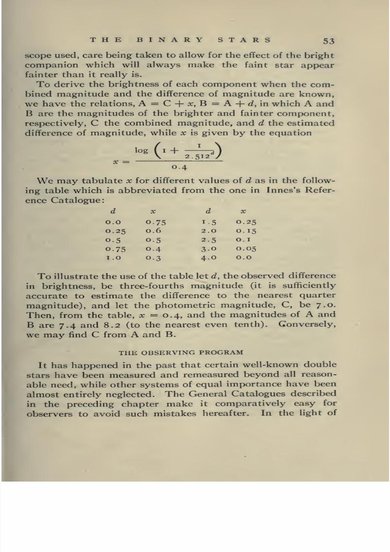
8/2/2019 The Binary Stars 1918
http://slidepdf.com/reader/full/the-binary-stars-1918 77/349
THE BINARY STARS 53
scope used, care being taken to allow for the effect of the bright
companion which will always make the faint star appear
fainter than it really is.
To derive the brightness of each component when the com-
bined magnitude and the difference of magnitude are known,
we have the relations, A = C + :x;, B = A + ^, in which A and
B are the magnitudes of the brighter and fainter component,
respectively, C the combined magnitude, and d the estimated
difference of magnitude, while x is given by the equation
log (i + -^'j\ 2512 /
X =0.4
We may tabulate x for different values of d as in the follow-
ing table which is abbreviated from the one in Innes's Refer-
ence Catalogue:
d X d X
0.0 0.75 1-5 0.25
0.25 0.6 2.0 0.15
0.5 0.5 2.5 O.I
0.75 0.4 30 0.05
I.O 0.3 4.0 0.0
To illustrate the use of the table letd,
the observeddifference
in brightness, be three-fourths magnitude (it is sufficiently
accurate to estimate the difference to the nearest quarter
magnitude), and let the photometric magnitude, C, be 7.0.
Then, from the table, x = 0.4, and the magnitudes of A and
B are 7.4 and 8.2 (to the nearest even tenth). Conversely,
we may find C from A and B.
THE OBSERVING PROGRAM
It has happened in the past that certain well-known double
stars have been measured and remeasured beyond all reason-
able need, while other systems of equal importance have been
almost entirely neglected. The General Catalogues described
in the preceding chapter make it comparatively easy for
observers to avoid such mistakes hereafter. In the light of

8/2/2019 The Binary Stars 1918
http://slidepdf.com/reader/full/the-binary-stars-1918 78/349
54 THE BINARY STARS
the knowledge these catalogues give of past observations and
of the motions in the various systems, the observer who
wishes his work to be of the greatest possible value will
select stars which are suited to his telescope and which are in
need of measurement at a given epoch either because of scar-
city of earlier measures or because the companion is at a critical
point in its orbit. For example, I am measuring /3 395 = 82
Ceti regularly at present because there are no measures of the
companion in the part of the orbit through which it is now
moving, and I am watching e Equulei closely because at present
it is apparently single and the position of the companion at
the time of its reappearance will practically decide the char-
acter of the orbit.
It has often been said that a careful set of measures of any
pair of stars made at any time is valuable. Granting this to
be so, it is certain that its value is greatly enhanced if it is
made to contribute to the advancement of a program havinga definite end in view. If the aim is to increase the number
of known orbits as rapidly as possible, attention should be
centered upon the closer pairs, particularly those under 0.5"
and those which have already been observed over considerable
arcs of their orbits. I am emphatically of the opinion that
it is wise for an observer possessing the necessary telescopic
equipment to devote his energy to the measurement of alimited number of such systems, repeating the measures every
year, or every two or five years, as may be required by the
rapidity of the orbital motion, for a long series of years. Such
a series can be investigated for systematic as well as acciden-
tal errors of measure far more effectively than an equal num-
ber of measures scattered over a much larger program, and
will add more to our real knowledge of the binary systems.
The wider pairs, and particularly those in the older catalogues,
now need comparatively little attention, so far as orbital mo-
tion is concerned. Even moderately close pairs, with distance
from i" to 5", need, in general, to be measured but once in
every ten or twenty years. Useful programs, however, may
be made from wider pairs for the detection of proper motions,
or for the determination of the relative masses in binary sys-

8/2/2019 The Binary Stars 1918
http://slidepdf.com/reader/full/the-binary-stars-1918 79/349
THE BINARY STARS 55
terns by means of measures connecting one of the components
with one or more distant independent stars. Photography is
well adapted to such programs.It is hardly necessary to add that an hour in the dome on
a good night is more valuable than half a dozen hours at the
desk in daylight. Everything possible should therefore be
done to prevent loss of observing time. In this connection I
have found charts based on the Durchmusterung invaluable
for quick identification of stars.
THE RESOLVING POWER OF A TELESCOPE
It has been shown that the diffraction pattern of the image
of a point source of light, like a star, formed by a lens "is a
disk surrounded by bright rings, which are separated by cir-
cles at which the intensity vanishes."^
Schuster gives the formula
p = m — (5)
in which p is the radius of a circle of zero intensity (dark ring),
D the diameter of the lens,/ its focal length, X the wave length
of the light from the point source, and m a coefficient that
must be calculated for each ring. For the first dark ring it is
1.220, and the values for the successive rings increase by very
nearly one unit. Nearly all of the light (0.839) is in the cen-
tral disk, and the intensity of the bright difi*raction rings
falls off very rapidly. Now it is generally agreed that the
minimum distance at which a double star can be distinctly
seen as two separate stars is reached when the central disk of
the image of the companion star falls upon the first dark ring
of the image of the primary, and the radius of this ring, ex-
pressed in seconds of arc, is therefore frequently called thelimit of the telescope's resolving power. If we adopt for X
the wave length 5,500 Angstrom units, the expression for pin
angular measure becomes
P=-^ (6)
' Schuster, Theory of Optics (1904), p. 130.

8/2/2019 The Binary Stars 1918
http://slidepdf.com/reader/full/the-binary-stars-1918 80/349
56 THE BINARY STARS
from which the resolving power of a telescope of aperture D(in inches) may be obtained. For the thirty-six-inch Lick
refractor, the formula gives 0.14", for the twelve-inch, 0.42".
It will be observed that the resolving power as thus derived
rests partly upon a theoretical and partly upon an empirical
basis. When the central disk of each star image of a pair falls
upon the first dark ring of the other image, the intensity curve
of the combined image will show two maxima separated by a
distinct minimum. When the disks fall closer together this
minimum disappears, the image becomes merely elongated,
perhaps with slight notches to mark the position of the dis-
appearing minimum. The pair is now no longer 'resolved'
according to the definition given but to the experienced
observer its character may still be unmistakable. For ex-
ample, in the Lick Observatory double star survey, Hussey
and I have found with the thirty-six-inch at least 5 double
stars with measured distances of o.ii" or less, the minimum
for each observer being 0.09"; and we have found many pairs
with the twelve-inch telescope whose distances, measured
afterward with the thirty-six-inch, range from 0.20" to
0.25". In all these cases the magnitudes were, of course,
nearly equal.
Lewis has published * a very interesting table of the most
difficult double stars measured and discovered by various ob-
servers using telescopes ranging in aperture from four inches
to thirty-six inches. He tabulates in separate columns the
values for the 'bright' and 'faint' pairs of nearly equal magni-
tude, and for the bright and faint pairs of unequal magnitude,
each value representing the mean of 'about five' of the closest
pairs for a given observer and telescope. A final column
adds the theoretical resolving power derived, not from the
equation given above, but from Dawes's well-known empirical
formula—resolving power equal 4.56" divided by the aperture
in inches (a)—which assumes the two stars to be of about
the sixth magnitude. Lewis finds that, in general, this for-
mula gives values which are too small even for the 'bright equal
The Observatory, vol. xxxvii, p. 378, 1914.

8/2/2019 The Binary Stars 1918
http://slidepdf.com/reader/full/the-binary-stars-1918 81/349
THE BINARY STARS 57
pairs', and he suggests the following as representing more
precisely the results of observation
4.8"Equal bright pairs
, mean magnitudes 5.7 and 6.4a
8 s"Equal faint pairs —'
, mean magnitudes 8.5 and 9.1a
Unequal pairs —'— , mean magnitudes 6,2 and 9.5a
Very unequal pairs
—'
—,
mean magnitudes 4.7 and 10,4a
Lewis is careful to state that his table does not necessarily
represent the minimum limits that may be reached with a
given telescope under the best conditions, and I have just
shown that they do not represent the limits actually reached
at the Lick Observatory. Taking from each of the three lists
of new double stars /8 1,026 to jS 1,274, Hu i to Hu 1,327, and
A I to A 2,700, 'about five' of the closest bright, and closest
faint, equal pairs discovered by each of the three observers,
Burnham, Hussey, and Aitken—29 pairs in all—I find the
following formulae for the thirty-six-inch telescope:
Equal bright pairs —^— , mean magnitudes 6.9 and 7.1
a
61"Equal faint pairs —'
, mean magnitudes 8.8 and 9.0
a
The most interesting point about these formulae is that
they show much less difference between the values for faint
and bright pairs than Lewis's do.
While it is a matter of decided interest to compare the limits
actually attained with a given telescope with the theoretical
resolving power, an observer, in making out his working pro-
gram for double star measurement, will do well to select
pairs that run considerably .above such limiting distances.
My deliberate judgment is that, under average good observing
conditions, the angular separation of the pairs measured should
be nearly double the theoretical limit. Observers with the
most powerful telescopes, however, are confronted with the

8/2/2019 The Binary Stars 1918
http://slidepdf.com/reader/full/the-binary-stars-1918 82/349
58 THE BINARY STARS
fact that if they do not measure the very closest known pairs
these must go unmeasured.
EYE-PIECES
The power of the eye-piece to be used is a matter of practical
importance, but one for which it is not easy to lay down spe-
cific rules. The general principle is use the highest power the
seeing will permit. When the seeing is poor, the images 'dan-
cing' or 'blurred', increase in the magnifying power increases
these defects in the images and frequently more than offsets
in this way the gain from increase in the scale. On such
nights, if they are suitable for any work, choose wider pairs
and use lower powers. The practical observer soon realizes
that it is not worth while to measure close pairs except with
high powers. With the thirty-six-inch telescope my own
practice is to use an eye-piece magnifying about 520 diameters
for pairs with angular separation of 2" or more. If the dis-
tance is only i ", I prefer a power of i ,000, and for pairs under
0.5", I use powers from 1,000 to 3,000, according to the angular
distance and the conditions. Closeness and brightness of the
pair and the quality of the definition are the factors that de-
termine the choice. Very close pairs are never attempted un-
less powers of i ,500 or higher can be used to advantage.
The simplest method of measuring the magnifying power of
an eye-piece in conjunction with a given objective is to find
the ratio of the diameter of the objective to that of its image
formed by the eye-piece—the telescope being focused and
directed to the bright daylight sky. Two fine lines ruled on a
piece of oiled paper to open at a small angle form a convenient
gage for measuring the diameter of the image. A very small
error in this measure, however, produces a large error in the
ratio and the measure should be repeated many times and the
mean result adopted.
DIAPHRAGMS
It is sometimes said that the quality of star images is im-
proved by placing a diaphragm over the objective to cut down
its aperture. I question this. It is certain that the experience

8/2/2019 The Binary Stars 1918
http://slidepdf.com/reader/full/the-binary-stars-1918 83/349
THE BINARY STARS 59
of such observers as Schiaparelli and Burnham is directly
opposed to it, and experiments made with the twelve-inch and
thirty-six-inch telescopes offer no support for it. Indeed, it
is difficult to understand how cutting ofif part of the beam of
light falling upon an object glass of good figure can improve
the character of the image, unless it is assumed that the ampli-
tude of such atmospheric disturbances as affect the definition
is small enough to enter the problem. The only possible gain
might be in the reduction of the brightness of the image when
one star of apair is
exceptionally bright, as in Sirius; but thisreduction can be effected more conveniently by the use of
colored shade glasses over the eye-piece. These are occasion-
ally of advantage.
A hexagonal diaphragm placed over the objective, however,
may prove of great value in measuring stars, like Sirius or
Procyon, which are attended by companions relatively very
faint; but this is because such a diaphragm entirely changes
the pattern of the diffraction image of the star, not because
it cuts down the aperture of the telescope. The pattern is
now a central disk from which six thin rays run ; between these
rays the field appears dark even close to the bright star, and
a faint object there can be seen readily that would be invisible
otherwise. Professor Barnard ^ has used such a diaphragm to
advantage with the forty-inch Yerkes refractor. Provision
should be made for rotating the diaphragm through an angle
of about 60° and it will be convenient in the case of a large
instrument to be able to do this by means of gearing attached
to a rod running down to the eye-end.
ERRORS OF OBSERVATION
All measures of angles or of distances are affected by errors,
both accidental and systematic, and when, as in double star
work, the measured quantities are very minute, these errors
must be most carefully considered. The accidental errors
may be reduced by careful work and by repeating the mea-
sures a suitable number of times. Little is to be gained, in this
respect or in any other, by making too large a number of set-
' A. N., vol. clxxxii, p. 13, 1909.

8/2/2019 The Binary Stars 1918
http://slidepdf.com/reader/full/the-binary-stars-1918 84/349
6o THE BINARY STARS
tings upon an object on any one night; because such factors
as the seeing, the hour angle, the observer's physiological con-
dition, all remain nearly constant. As a rule, four settings for
position angle and three or even two measures of double dis-
tance are enough to make on one night, but the measures
should be repeated on one or more additional nights. This is
not only to reduce the accidental error of measure but to
guard against outright mistakes in reading the circles, record-
ing, etc. As to the number of nights on which a system should
be measured at a given epoch, opinions will differ. Some ob-
servers run to excess in this matter. Generally, it may be said
that it is time wasted to measure a system on more than four
nights at any epoch and ordinarily the mean of three nights'
measures, or even of two, if the pair is easy to measure and the
measures themselves are accordant, is as satisfactory as the
mean from a larger number. In critical cases, however, a
larger number is sometimes desirable.
The systematic errors of measurement are far more trouble-
some, for they vary not only with the individual but are dif-
ferent for the same observer at different times and for different
objects. Aside from the personality of the observer, they
depend upon the relative magnitudes of the two components
of a double star, the angular distance, the angle which the line
joining the stars makes with the horizontal, and, in unequal
pairs, upon the position of the faint star with respect to the
bright one. Various methods have been adopted to deter-
mine these errors or to eliminate them.
The most elaborate investigation in this line is probably
that made by Otto Struve, who measured "artificial double
stars formed by small ivory cylinders placed in holes in a black
disk." He deduced formulae by means of which he calculated
corrections to be applied to all of his measures; but it is very
doubtful whether these corrections really improve the results.
I agree with Lewis when he says, "I would prefer his original
measures—in part because the stars were so particularly arti-
ficial." The actual conditions when observing the stars at
night are of necessity widely different from those under which
the test measures were made. Certainly, in the case of Otto

8/2/2019 The Binary Stars 1918
http://slidepdf.com/reader/full/the-binary-stars-1918 85/349
THE BINARY STARS 6i
Struve, the 'corrected' angles and distances are frequently
more at variance with the general run of all of the measures
by good observers than the original values. The student of
double star motions will generally find it advantageous to use
the original uncorrected measures of every observer in his pre-
liminary work and then to derive values for the systematic
or personal errors of each by comparing his measures with
the curve representing the means of all available measures.
The observer, on the other hand, may profitably adopt
observing methodsdesigned
to eliminate,in
part atleast,
systematic errors. Innes's plan of measuring each pair on
each side of the meridian is an excellent one because, in gen-
eral, the line joining the two stars changes its angle with respect
to the horizon in passing the meridian. In the extreme case,
if the smaller star is above the primary when the pair is east
of the meridian, it will be below, when west of the meridian.
When Innes's two measures made in this way are not
sufficiently accordant, he repeats them on two additional
nights, one night in each position of the instrument.
In 1908, MM. Salet and Bosler ^ published Jthe results of an
investigation of the systematic errors in measures of position
angle in which they made use of a small total reflecting prism
mounted between the eye-piece and the observer's eye and
capable of being rotated in such manner as to invert the field
of view. Theoretically, the half sum of the measures made
without and with the prism should represent the angle freed
from errors depending upon the inclination of the images to
the horizon. In fact, Salet and Bosler found that, whereas
their measures without the prism and those made with it both
showed a personal equation varying in amount with the star,
the means of the two sets were remarkably free from person-
ality. Here, for example, are their measures of 7 Leonis:
Observer Date Without Prism With Prism Mean
Salet
Bosler
(S-B)
1907.19
1907.23
119.04°
116.80°
+2.24°
113.50°
116.07°
-2.57°
116.27°
116.44°
-0.17°
• Bulletin Astronotnique, Tome p. 18, 1908.
8/2/2019 The Binary Stars 1918
http://slidepdf.com/reader/full/the-binary-stars-1918 86/349
62 THE BINARY STARS
Hermann Struve and J. Voiite have since published mea-
sures made in this manner and each concludes that the results
are far better than his meaures made entirely without the useof the prism. In M. Votlte's last paper ^ the statement is
made that "it is principally in observing in the perpendicular
(:) position that the observations show a pronounced syste-
matic error," while "the parallel ( . . ) observations are in gen-
eral free from systematic errors."
Dawes ^ long ago pointed out that in "rather close double
stars," the measures of distance "will almost inevitably be
considerably too large" unless the observer has taken into
account the change made in the apparent form of the star
disk when a thread of the micrometer is placed over it.
This change is in the nature of a swelling out of the disk
on each side of the thread, producing an approximately
elliptical disk. When two images are nearly in contact and
the threads are placed over them this swelling obliterates
the interval between the disks and the threads are therefore
set too far apart. The effect disappears when the disks are
well separated.
In my investigations of double star orbits I have frequently
noticed that distance measures of a given system made with
small apertures are apt to be greater than those made with
large telescopes even when made by the same observer, pro-
vided the system is a close one as viewed in the smaller instru-
ment. I have found such a systematic difference in the dis-
tances in stars which I have measured with the twelve-inch
and with the thirty-six-inch telescope, and Schlesinger ^ has
also called attention to this difference, giving a table derived
from my measures as printed in Volume XII of the Publi-
cations of the Lick Observatory. This table is here reproduced
with a column of differences added
''Circular No. 27, Union Observatory, South Africa, 191 S.
• Mem. Royal Astronomical Society, vol. xxxv, p. I53i 1867.
'Science, N. S., vol. xliv, p. S73t 1916.

8/2/2019 The Binary Stars 1918
http://slidepdf.com/reader/full/the-binary-stars-1918 87/349
THE BINARY STARS
Measured Separations
63
Number of
Stars
With the
12-inch
With the
36-inchDifiference
20 0.52" 0.42" -fo.io''
25 0.62" 0.54" +0.08*'
20 0.71'' 0.64" +0.07'
24 0.81" 0.79" +0.02"
24 1.07^ 1.03'' +0.04*'
21 1.38" 1.39' —O.OI"
26 2.13'' 2.10" +0.03"18 449" 4.53" —0.04'
The systematic difference is clearly shown in all the pairs
having a separation less than twice the resolving power (042")
of the twelve-inch telescope ; in the wider pairs it is negligibly
small.
Occasionally an observer's work shows systematic differ-
ences of precisely the opposite sign. Thus Schlesinger (/. c.)
shows that in Fox's recent volume ^^ of double star observa-
tions the distances are measured smaller with the twelve-inch
than with the eighteen and one-half-inch or with the forty-
inch, "the differences being largest for small separations and
becoming negligibly small for separations in the neighborhood
of 5"." The personal equation revealed in such comparisons
as these must obviously be taken into account in orbit com-
putations.
PHOTOGRAPHIC MEASURES
Photographic processes of measurement are coming more
and more into favor in almost all lines of astronomical work,
and with the constant improvements that are being made in
the sensitiveness and fineness of grain in the plates it is prob-
able that important work in double star measurement will
soon be undertaken photographically. Indeed, experiments
in this line date back to 1857, when G. P. Bond secured with
an eight-second exposure on a collodion plate the first mea-
surable images of a double star—f Ursae Majoris, angular
^^ Annals of the Dearborn Observatory, Northwestern University, vol. i, 191S.

8/2/2019 The Binary Stars 1918
http://slidepdf.com/reader/full/the-binary-stars-1918 88/349
64 THE BINARY STARS
separation 14.2". Pickering and Gould in America, MM.Henry in France, and the Greenwich observers in England,
among others, followed up this early attempt and succeeded
in securing results of value for some stars as close as i ". More
recently Thiele, Lau, and Hertzsprung at Copenhagen have
carried out more extensive programs and have investigated
several possible sources of systematic error in the measure-
ment of photographic plates. Hertzsprung is at present con-
tinuing his researches at Potsdam, and finds it possible to
secure excellent measures of pairs as close as i ".
There are obvious limitations to the application of photog-
raphy to double star measurement; very close pairs and pairs
with moderate distances in which one component is relatively
faint will not give measurable images on plates at present
available. On the other hand there is no question but that
wider pairs can be as accurately, and far more conveniently
measured photographically than visually, provided systematicerrors are eliminated. The discovery of faint double stars
with distances exceeding, say 3^, may also with advantage be
left to the photographic observer. Comparison under the
blink microscope of plates taken at suitable intervals with
instruments giving fields on the scale of the Carte-du-ciel charts
will quickly reveal any such pairs which show appreciable
motion and these are the only faint pairs that need be takeninto serious account in the present stage of double star astron-
omy. Instruments giving photographs of larger scale will, of
course, reveal closer pairs. Thus, Fox, on plates exposed with
the eighteen and one-half-inch Dearborn refractor, has recently
found two pairs (Fox 11 and Fox 25) with measured distances
of 1.7" and 1.2", the magnitudes being 9.9—ii.o and 9.6—10.2
respectively.

8/2/2019 The Binary Stars 1918
http://slidepdf.com/reader/full/the-binary-stars-1918 89/349
CHAPTER IV
THE ORBIT OF A VISUAL BINARY STAR
We have seen that Sir William Herschel, by his analysis of
the observed motion in Castor and other double stars, demon-
strated that these systems were "real binary combinations of
two stars, intimately held together by the bonds of mutual
attraction." Later observation has shown that the apparent
motion in such systems is on the arc of an ellipse and that the
radius vector drawn from the primary star to its companion
sweeps over areas which are proportional to the times. It has
therefore been assumed from the beginning that the attractive
force in the binary star systems is identical with the force of
gravitation in our solar system, as expressed by Newton's law,
and the orbit theories which we are to investigate in the present
chapter are all based upon this assumption. Before taking
up the discussion of these theories it is pertinent to inquire
whether the fundamental assumption is justified.
It is supported by all of the available evidence but rigorous
mathematical proof ofits validity is difficult because the
motion which we observe in a stellar system is not the true
motion but its projection upon a plane perpendicular to the
line of sight. The apparent orbit is therefore, in general, not
identical with the true orbit and the principal star may lie at
any point within the ellipse described by the companion and
not necessarily at either the focus or the center. Hence, in
Leuschner's words, "mathematical difficulties are encountered
in establishing a law of force which is independent of the angle
B, the orientation." In the article quoted, Leuschner, after
pointing out that "Newton did not prove the universality of
the law of gravitation, but by a happy stroke of genius gener-
alized a fact which he had found to be true in the case of the
mutual attraction of the Moon and the Earth," proceeds to
show that the law does hold throughout the solar system, the

8/2/2019 The Binary Stars 1918
http://slidepdf.com/reader/full/the-binary-stars-1918 90/349
66 THE BINARY STARS
question of orientation not entering. He then says that, in
binary systems, "when the law is arbitrarily assumed to be
independent of the orientation, as was found to be the case in
the solar system, two possibilities arise, namely, either that
the force is in direct proportion to the distance r between the
two stars or that the Newtonian law applies. It can be shown,
however, that when, in the case of an elliptic orbit, the force
is proportional to r, the primary star must be in the center of
the ellipse. As this has never been found to be the case, the
only alternative is the Newtonian law."
It should be clearly understood that the difficulty in demon-
strating the universality of the law of gravitation here pointed
out is purely mathematical. No physical reason has ever been
advanced for a dependence of an attracting central force upon
the orientation, and until such dependence has been proved
we may safely proceed with our investigation of binary star
orbits under the action of the law of gravitation.
Until the relative masses of the two components are known
it is impossible to determine the position of the center of
gravity of the system and we are therefore unable to compute
the orbits described by the two stars about that center. What
our measures give us is the apparent orbit of one star, the
companion, described about the other, the primary, which is
assumed to remain stationary at the focus.It is clear
thatthis relative orbit differs from the actual orbits of the two com-
ponents only in its scale.
The problem of deriving such an orbit from the micrometer
measures of position angle and distance was first solved by
Savary,^ in 1827, but Encke ^ quickly followed with a different
method of solution which was somewhat better adapted to
the needs of the practical astronomer, and Sir John Herschel ^
communicated a third method to the Royal Astronomical
Society in 1832. Since then the contributions to the subject
have been many. Some consist of entirely new methods of
attack, others of modifications of those already proposed.
Among the more notable investigators are Villarceau, Madler,
1 Savary, Conn, des Temps, 1830; Encke, Berlin Jahrbuch, 1832; Herschel, Memoirs
of the Royal Astronomical Society, s, 171, 1833.

8/2/2019 The Binary Stars 1918
http://slidepdf.com/reader/full/the-binary-stars-1918 91/349
THE BINARY STARS 67
Klinkerfues, Thiele, Kowalsky, Glasenapp, Seeliger, Zwiers,
Howard, Schwarzschild, See, and Russell.
The methods of Savary and Encke utilize four complete
measures of angle and distance and, theoretically, are excellent
solutions of the problem; Herschel's method is designed to
utilize all the available data, so far as he considered it reliable.
This idea has commended itself to all later investigators.
Herschel was convinced, however, that the measures of dis-
tance were far less trustworthy than those of position angle,
and his method therefore uses the measures of distance simply
to define the semi-major axis of the orbit; all of the other
elements depend upon measures of position angle. At the time
this may have been the wisest course, but the distance mea-
sures of such early observers as W. Struve, Dawes, and Dem-
bowski, and those of later observers working with modern
micrometers, are entitled to nearly or quite as much weight as
the measures of position angle and should be utilized in theentire orbit computation.
Whatever method is adopted it is clear that the problem
consists of two distinct parts: first, the determination of the
apparent ellipse from the data of observation; secondly, the
derivation of the true orbit by means of the relations between
an ellipse and its orthographic projection.
THE appare;^t ellipse
Every complete observation of a double star supplies us with
three data: the time of observation, the position angle of the
companion with respect to the primary, and the angular dis-
tance between the two stars. It is clear, as Comstock pointed
out many years ago, that the time of observation is known
with far greater accuracy than either of the two coordinates
of position. The relations between the times of observation
and the motion in the ellipse should therefore be utilized ; that
is, the condition should be imposed that the law of areal veloc-
ity must be satisfied as well as the condition that the points of
observation should fall approximately upon the curve of an
ellipse. Elementary as this direction is, it is one that has been
neglected in many a computation.

8/2/2019 The Binary Stars 1918
http://slidepdf.com/reader/full/the-binary-stars-1918 92/349
68 THE BINARY STARS
Theoretically, the first step in our computation should be the
reduction of the measured coordinates to a common epoch by
the application to the position angles of corrections for pre-
cession and for the proper motion of the system. The distance
measures need no corrections. Practically, both corrections
are negligibly small unless the star is near the Pole, its proper
motion unusually large, and the time covered by the observa-
tions long. The precession correction, when required, can be
found with sufBcient accuracy from the approximate formula
A0= —0.0056° sin a sec 5 {t—to). (i)
The formula for the correction due to the proper motion of
the system is
A^= /x"sin 5 (/-/o) (2)
where m" is the proper motion in right ascension expressed in
secondsof arc.
When the measures of any binary star have been tabulated
(with the above corrections, if required) they will exhibit
discordances due to the accidental and systematic errors of
observation and, occasionally, to actual mistakes. If they were
plotted, the points would not fall upon an ellipse but would
be joined by a very irregular broken line indicating an ellipse
only in a general way. It will be advisable to investigate the
measures for discordances before using them in the construc-
tion of the apparent ellipse and the simplest method is to plot
upon coordinate paper first the position angles and then the
distances, separately, as ordinates, against the times of obser-
vation as abscissae, using a fairly large scale. Well determined
points (for example, a point resting upon several accordant
measures by a skilled observer and supported by the preceding
and following observations) may be indicated by heavier
marks. Smooth free-hand curves, interpolating curves, are
now to be drawn to represent the general run of the measures
and in drawing these curves more consideration will naturally
be given to the well observed points than to the others. Obser-
vations which are seriously in error will be clearly revealed and
these should be rejected if no means of correcting them is

8/2/2019 The Binary Stars 1918
http://slidepdf.com/reader/full/the-binary-stars-1918 93/349
THE BINARY STARS 69
available. The curves will also show whether or not the
measures as a whole are sufficiently good to make orbit com-
putation desirable.
If the amount of available material warrants it, the question
of the systematic or personal errors of the observers should
also be considered at this time. No reliable determination of
such errors is possible unless (a) measures by the same observer
under essentially the same conditions in at least four or five
different years are at hand, and (b) unless the total number of
measures by many different observers is sufficient to establish
the general character of the curves beyond reasonable question.
If the second condition is satisfied, the average of the residuals
from the curve for a given observer may be regarded as his
personal error and the corresponding correction may be applied
to all of his measures. Two further points should be noted:
Firsty the residuals in position angle should be reduced to arc
by multiplying by the factor p ^ 57.3 before the mean is taken,to allow for the effect of variations in the angular separation
second, the corrections should not be considered as constant
over too long a period of time. Many computers take no
account of the personal errors in their calculations, and if the
object is merely to obtain a rough preliminary orbit this prac-
tice is perhaps legitimate.
After all corrections have been applied, the measures which
are retained should be combined into annual means or into
mean places at longer or shorter time intervals according to
the requirements of the particular case. Several factors really
enter into the question of the weights to be assigned to the
individual observations in forming these means; for instance,
the size of the telescope used, the observing conditions, the
number of nights of observation, and the experience of the
observer; but it will be wise, in general, to disregard all but
the number of nights of observation, provided the telescope
used is of adequate resolving power for the system in question
and that the observer has not specifically noted some of his
measures as uncertain. A single night's measure deserves
small weight; mean results based upon from two to six nights'
accordant measures may be regarded as of equal weight; means
8/2/2019 The Binary Stars 1918
http://slidepdf.com/reader/full/the-binary-stars-1918 94/349
70 THE BINARY STARS
depending upon a much larger number of measures may be
weighted higher. In general, a range in weights from one to
three will be sufficient.
Having thus formed a series of normal places, we may find
the apparent ellipse which best represents them either graphi-
cally or by calculating the constants of the general equation
of the ellipse with the origin at any point. This equation is
ax^-\-2hxy-\-by^-\-2gx-]-2fy+c = o (3)
which may be written in the form
Ax^-{-2Hxy+Bf-\-2Gx-\-2Fy+i=o (4)
in which we must have A>o, B>o, and AB — IP>o.If we assume the position of the primary star as origin we
may calculate the five constants of this equation from as many
normal places by the relations
y= P cos u
but it is advisable to make a least squares solution using all of
the normal places.
The great objection to this method is that it entirely disre-
gards the times of observation. Moreover, the errors of obser-
vation, small as they are numerically, are large in proportion
to the quantities to be measured, a fact which makes it difficult
to obtain a satisfactory ellipse without repeated trials. The
graphical methods are therefore to be preferred.
The simplest method, and one that in most cases is satis-
factory, is to plot the positions of the companion star in polar
coordinates, the primary star being taken as the origin. With
the aid of an ellipsograph or by the use of two pins and a
thread, an ellipse is drawn through the plotted points and is
adjusted by trial until it satisfies the law of areas. This adjust-
ment must be made with the greatest precision and the curve of
the ellipse drawn with great care, for the construction of the
apparent ellipse is the critical part of the entire orbit deter-
mination. In my own practice I have found that the test for
the law of areas can be made most rapidly by drawing radii
to selected points which cover the entire observed arc and

8/2/2019 The Binary Stars 1918
http://slidepdf.com/reader/full/the-binary-stars-1918 95/349
THE BINARY STARS 71
measuring the corresponding elliptic sectors with a planimeter.
The comparison of the areal velocities derived from the dif-
ferent sectors at once indicates what corrections the ellipse
requires. With a suitable ellipsograph a new ellipse is quickly-
drawn and the areas again measured. The process is repeated
until a satisfactory ellipse has been obtained.
Some investigators still prefer the mode of procedure in
constructing the apparent ellipse first suggested by Sir John
Herschel. An interpolating curve is drawn, in the manner
described above, for the position angles only, using the meanor normal places. If the curve is carefully drawn, smoothly
and without abrupt changes of curvature, it should give the
position angle for any particular epoch more accurately than
the measure at that epoch, for it rests upon all of the measures.
From this curve read the times corresponding to, say, every 5°
of angle, tabulate them, and take the first differences. Divid-
ing these by the common angle difference will give a series of
dt
approximate values of -— . But by the theory of elliptic motiondu
p2 -— must be a constant and hence p = c ^ \ Therefore adt
'^
\ide
series of relative values of the distance (expressed in any con-
venient unit) corresponding to every fifth degree of position
angle can be derived from the table of angles. Now plot the
points representing corresponding angles and relative dis-
tances; if the interpolating curve has been correctly drawn
and read off they will all lie upon the arc of an ellipse. If they
do not, draw the best possible ellipse among them and use it
to correct the interpolating curve, repeating the process until
the result is satisfactory. Finally, convert the relative into
true distances by comparing those distance measures whichare regarded as most reliable with the corresponding values in
the unit adopted in the plot.
There are at least two objections to this method: First, it
does not make adequate use of the observed distances; and
second, when the angle changes rapidly, as it does in many
systems at the time of minimum apparent separation, it is
almost impossible to draw the interpolating curve correctly.

8/2/2019 The Binary Stars 1918
http://slidepdf.com/reader/full/the-binary-stars-1918 96/349
72 THE BINARY STARS
In my judgment, It is far better to plot directly the normal
positions given by the observed angles and distances and then
by the method of trial and error to find the ellipse which best
represents them and at the same time satisfies the law of areas.
THE TRUE ORBIT
After the apparent ellipse has been constructed graphically,
or from the constants in the equation of the ellipse, it remains
to derive the elements which define the form and size of the
true orbit, the position of the orbit plane, the position of theorbit within that plane, and the position of the companion
star in the orbit at any specified time. Some confusion in the
nomenclature and even in the systems used in defining these
elements has arisen from the fact that it is impossible to say,
from the micrometer measures alone, on which side of the
plane of projection (which is taken as the plane of reference)
the companion star lies at a given time. In other words,
wecannot distinguish between the ascending and the descending
node, nor between direct and retrograde motion in the ordinary
sense. Further, in some systems the observed position angles
increase with the times, in others they decrease.
The following system is adopted as most convenient when
the requirements of the observer of radial velocities are con-
sidered as well as those of the observer with the micrometer.
In the details in which it differs from other systems in use, it
was worked out by Dr. Campbell in consultation with Professor
Hussey and the present writer.
Let
P= the period of revolution expressed in mean solar years.
r=the time of periastron passage.
e= the eccentricity,
o= the semi-axis major expressed in seconds of arc.
fl= the position angle of that nodal point which lies between o° and
1 80°; that is, the position angle of the line of intersection of
the orbit plane with the plane perpendicular to the line of
sight. Call this merely "the nodal point", disregarding the
distinction between ascending and descending nodes.
CO= the angle in the plane of the true orbit between the line of nodes
and the major axis. It is to be measured from the nodal point

8/2/2019 The Binary Stars 1918
http://slidepdf.com/reader/full/the-binary-stars-1918 97/349
THE BINARY STARS 73
to the point of periastron passage in the direction of the com-
panion's motion and may have any value from 0° to 360°. It
should be stated whether the position angles increase or de-crease with the times.
i= the inclination of the orbit plane; that is, the angle between the
orbit plane and the plane at right angles to the line of sight.
Its value lies between 0° and ±90° and should always carry
the double sign (dz) until the indetermination has been re-
moved by measures of the radial velocity. When these are
available, i is to be regarded as positive (+) if the orbital
motion at the nodal point is carrying the companion star awayfrom the observer; negative, if it is carrying the companion
star towards the observer.
The symbol n denotes the mean annual motion of the com-
panion, expressed in degrees and decimals, measured always in
the direction of motion.
There is no difference of opinion in regard to the definition
of the first four elements; the conventions of taking Q. always
less than 180° and of counting co (for which many computers
use the symbol X) always in the direction of the companion's
motion were first suggested, I believe, by See, and have been
adopted by Burnham, Hussey, Aitken and others. The defini-
tion of i (for which some computers write 7) is the usual one,
but computers, as a rule, do not use the double sign. Many
also prefer to count the mean annual motion in the direction
of increasing position angles in all systems, and to consider the
motion negative when the angles decrease with the times.
When the elements are known, the apparent position angle
6 and the angular distance p for the time / are derived from
the following equations
M=36o7P
M=^i{t-T) =E-esmEr =a{i—ecosE) (6)
tsin)4v= ^ l^ tan^E\i-e
tan {d—Q) = rbtan (I'+co) cos i
p = r cos {v-\-(jt)) sec {d—Q)(7)

8/2/2019 The Binary Stars 1918
http://slidepdf.com/reader/full/the-binary-stars-1918 98/349
74 THE BINARY STARS
Equations (6) are the usual ones for elliptic motion, the
symbols M, E, and v representing respectively, the mean,
eccentric, and true anomaly, and r the radius vector. Equa-tions (7) convert the v and r of the companion in the true
orbit into its position angle and distance in the projected, or
apparent orbit. Position angles are generally recorded only to
the nearest tenth of a degree in orbit computation, hence it is
sufficiently exact to take the value of E corresponding to a
given value of M from Astrand's Hiilfstafeln, which hold
for all values of the eccentricity, or the value of v directly
from the still more convenient Allegheny Tables, provided the
eccentricity does not exceed 0.77. If the latter tables are used
it is convenient to derive the value of r from the equation
r= a {i—e~) /(i+^cosiO (6a)
instead of from the third of (6).
kowalsky's method
From the many methods which have been devised for deriv-
ing the elements of the true orbit from the apparent ellipse I
have selected two to present in detail, Kowalsky's and Zwiers's.
Both are of very general application and are very convenient
in practice but there are cases in which both fail. Some of
these will be discussed on a later page.
Kowalsky's method ^ is essentially analytical and employs
the constants of the general equation of the ellipse.
Ax^ + 2 Hxy + By^-{-2Gx-\-2Fy+i =0. (4)
This is the equation for the rectangular projection of the
true orbit, the focus of the true orbit falling upon the position
of the principal star at the origin of coordinates for the ap-
parent ellipse. Equation (4) may also be regarded as the
equation of a right cylinder whose axis coincides with the
2-axis of the system of coordinates, that is, the line of sight.
Let this equation be referred to a new system of coordinates,
x\ y', z' , with the same origin, but with the :!c'-axis directed
2 First published, according to Glasenapp, in the Proceedings of the Kasan Imperial
University, 1873. This volume has not been accessible to me.

8/2/2019 The Binary Stars 1918
http://slidepdf.com/reader/full/the-binary-stars-1918 99/349
THE BINARY STARS 75
to the nodal point, and the ^''-axis at right angles to it in the
plane of the true orbit. Our transformation equations are
x= x' cos 12—y sin fl cos i-\-z' sin Q, sin i
y= x' sin fi+v' cos Q. cos i—z' cos 12 sin i (8)
s= H-y sin^' +3' cos i
Substituting these values in (4) and placing 2' = o, we shall
have the equation of the intersection of the cylinder with the
plane of the true orbit; that is, the real ellipse. Omitting
accents the equation now becomes
A {x cos 12— 3' sin fl cos iY
+ 2 i? (x cos 12 — >» sin 12 cos i) {x sin 12 + 3' cos 12 cos i)
+ 5 (x sin 12 + y cos 12 cos iY + 2 G (x cos 12 — y sin 12 cos i)
+ 2 F (x sin 12 + 3; cos 12 cos i) -{• i = o. (9)
Now the equation of the true ellipse referred to the focus
{i. e., the position of the principal star) as origin is
^ 4- I = o (10)
the X-axis coinciding with the major axis of the ellipse. Let us
turn this axis back through the angle co, to make it coincide
with the line of nodes, by substituting for x and y, respectively,
the values xcosco+J'sinco, and — :x;sina)+3'cosw, and equation
(10) becomes
(xcoso)-\-ys{no}-{-aey.
(— xsinco + ^'coso))'' , .
-: — —- 4- —1=0. (11)
a^^
b^
Equations (11) and (9) are necessarily identical since each
represents the same ellipse referred to the same origin and the
same axes; therefore the coefficients of the like powers of x and
y must be proportional. Let/ be the factor of proportionality.
Then we shall have:
/( 11 =^cos2co + 5sin2 12 + i7sin2l2 (12)
\ a^ b^ /
^/sm^co
_^cos^coX
= (^ si^2^4.5cos212-if sin2l2) cos^i (13)
\ a^ b^ /

8/2/2019 The Binary Stars 1918
http://slidepdf.com/reader/full/the-binary-stars-1918 100/349
76 THE BINARY STARS
/( ) sin2a>=(—^sin2l2+-Ssin2Q4-2Hcos2n)cos'^i (14)\ a^ IP- J
^ecosco^c;(,osj2+Fsmfi (15)
a
/^^^^ = (-Gsinl2 + Fcosl2)cosi (16)
a
/ (6^-1) = + I. (17)
From (17) we find
I — e^
and hence, introducing the semiparameter, p = lPla, the
relation
J = = =, or, a = (17a)
We may now write (16) and (15) in the forms
— sin CO = — (Fcosfi— Gsintt) cost
p(18)
— cos CO = — (Fsin U-\- G cos 12).
P
Twice the product of equations (18) is
— sin 2 o) = {F^ sin 2 12 — G^ sin 2 12 4- 2 FG cos 2 12) cos i (19)
and equation (14) may be written
— sin 2 CO = (— ^ sin 2 12 + 5 sin 2 12 + 2 Hcos 2 12) cos i; (20)
hence
(F2 - G2 + ^ - 5) sin 2 n^2iFG-H) cos 2 12 = o. (21)
Subtracting (13) from (12) and substituting for — —
its equal —- we have
g2— cos 2 CO = ^ cos2 12 + -B sin2 12 + Hsin 2 12
^' - {A sin2 12 + 5 cos2 12 - iJ sin 2 12) cos^ I (22)

8/2/2019 The Binary Stars 1918
http://slidepdf.com/reader/full/the-binary-stars-1918 101/349
THE BINARY STARS 77
The difference of the squares of the two equations (i8) gives
another value of
— cos 2co.
Equating the two values and
solving for cos^i we obtain
2 . _ (P- B) sin'^n + {(P - A) cos^n-^ {FG - H) sin 2 12 .^^^^ *~
{F^- B) cos''n+ {G^ - A) siti^a- {FG - H) sm2d
It is obvious from the forms of the numerator and denomi-
Nnator of this equation that if we put cos^t= — and therefore
,. D-N D+N ^ „ ^tan^^ = = —-- — 2 we shall have
N N
tan2i= 2. (24)
N
g2 I
The first member of (13) may be written—-sin^co —^^"^the equation
— sin^o; -— = (A sin^ U -\- B cos^ ^ - H sin 2 12) cos^ i. (25)
/2 I
Squaring (16) and substituting for— its equal— we find
— sin2 03= (F^ cos2 12 + G^ ^1^2 ^ - PG sin 2 12) cos^ i; (26)
and from (25) and (26)
— = [(P-5)cos212+(G2-^)sin212-(FG-//)sin2l2]cosn\ (27)
Substituting the value of cos^i from (23) we have
— =(P-5)sin212+((7-^)cos212+(FG-H)sin2l2 = iV; (28)
therefore (24) may be written
2 tan^
^ ~7i^ =F^^Cp.^A + B). (29)

8/2/2019 The Binary Stars 1918
http://slidepdf.com/reader/full/the-binary-stars-1918 102/349
78 THE BINARY STARS
Writing for sin^ 12 and cos^ 12 in (28) the corresponding func-
tions of 2 12 we find
-^ = P+G2- U+5) -(P-J5)cos2l2^'
+ (G' - ^) cos 2 12+2 (FG-i/) sin 2 12. (30)
Therefore from (29) we have
r= {F" - C -\- A - B) COS2Q. - 2 {FG - H) sin 2 12. (31)
Multiply (31) by sin 2 12 and (21) by cos 2 12 and subtract thelatter result from the former. Then
^""'Sin 2 12 = - 2 {FG - m. (32)
Next multiply (31) by cos 2l2 and (21) by sin 2l2 and add the
products. We have
tan^^"
P'
cos 2 12 = F2 - G2 + ^ - jB. (33)
Equations (33), (32), (29), (18), and (17a) define the geo-
metric elements of the orbit in terms of the known constants
derived from the measures with the micrometer.
To complete the solution analytically the period P and the
time of periastron passage T will be found from the mean
anomalies M computed from the observations by taking the
ephemeris formulae on page 73 in the reverse order. Every
M will give an equation of the form
-^60°
M = -— (/- D, or, M = fit + e, where e = - fiT
and the two unknowns P and T will be computed from all the
equations by the method of least squares.
GLASENAPP'S MODIFICATION OF KOWALSKY's METHOD
In theory, Kowalsky's method leaves nothing to be desired;
given accurate measures it will lead to definitive results. But
the measures of a double star, as we know, are affected by
errors that are at present unavoidable, and, until means shall

8/2/2019 The Binary Stars 1918
http://slidepdf.com/reader/full/the-binary-stars-1918 103/349
THE BINARY STARS 79
be devised to eliminate these more completely than we are
now able to do, it will be more practical to adopt Glasenapp's
suggestion and derive the five constants of the equation of
the ellipse by his graphical method. Then we may apply
Kowalsky's formulae, as before, to find the geometric elements
of the orbit.
Glasenapp ^ assumes the apparent ellipse to have been
drawn. Let its equation be, as before,
Ax"^ + 2 Hxy + 5/ + 2 Gx + 2 F>' + I = o. (4)
Put3' = o; then the roots of the resulting equation
Ax'^-{-2Gx-{-i =0
will be the abscissae of the points of the orbit on the a£: = axis.
If we represent these roots by Xi and X2, we have, by the theory
of equations,
A= , and G = . (34)
Xi X2 2 Xi X2
Similarly, if we put x = o, we have the equation
By^ + 2Fy-{-i =0,
whose roots will be the ordinates of the points of the orbit on
the y = axis. From these we obtain
B=^,andf=-^^i+^. (35)
yi yi 2 >'i yi
Therefore, direct measurement of the distances from the prin-
cipal star to the intersections of the apparent ellipse with the
axes of X and y, care being taken to regard the algebraic signs,
will give the four constants A, B, G, and F. H, the remaining
constant, is derived from
Ax-'-\-By^'-i-2Gx-\-2 Fy+i . ^-n =
. k3^)2xy
Measure the coordinates of several points on the apparent
ellipse, choosing such as will make the product xy as large as
possible. Each set, substituted in (36) will give a value of H.
' Monthly Notices Royal Astronomical Society 40, 276, 1889.

8/2/2019 The Binary Stars 1918
http://slidepdf.com/reader/full/the-binary-stars-1918 104/349
80 THE BINARY STARS
The accordance of the separate values will depend upon the
care with which the ellipse has been drawn, and the mean of
all the values should be adopted.
Glasenapp's modifications practically convert Kowalsky's
analytical method into a graphical one for the values of P and
7", as well as the constants of the general equation which define
the purely geometrical elements, may be determined by mea-
sures of the apparent ellipse. It is most convenient to make
the measures for P and T with the aid of a planimeter as
followsThe position of the periastron point P is at that end of the
diameter of the apparent ellipse drawn through the origin 5
which is nearest the origin, for this diameter is clearly the
projection of the line of apsides of the true orbit. Having
determined the constant of areal velocity {c) from the portion
of the ellipse covered by the observations, we measure the
areas of two sectors, PSt, and PSt\ where t and /' represent
observed positions on either side of P. Divide these areas by
c and apply the quotients with the appropriate signs to the
times corresponding to t and /'. The two resulting values of
T, the time of periastron passage, should agree closely. More
points than two may, of course, be used and the mean of all
the values for T adopted. Similarly, the area of the entire
ellipse divided by c gives the value of the revolution period.
Since all the areas are simply relative it is not necessary to
know the unit of area.
ZWIERS'S METHOD
Many methods have been published that enable the com-
puter to derive the elements of the true orbit from graphical
constructions. It is impossible to discuss them all in this
chapter, and it is, fortunately, unnecessary. The crux of our
problem is the construction of the apparent ellipse; when this
has been accomplished, almost any of the methods which have
been proposed will give satisfactory preliminary elements,
provided the ellipse is a fairly open one. If it is very narrow
and greatly elongated, none of the ordinary methods is entirely

8/2/2019 The Binary Stars 1918
http://slidepdf.com/reader/full/the-binary-stars-1918 105/349
THE BINARY STARS 8l
satisfactory. I have selected Zwiers's * method for presenta-
tion here because it is as simple as any and is one which I have
found very convenient.
Zwiers assumes the apparent ellipse to have been drawn.
Since it is the projection of the true orbit, the diameter which
passes through the primary star's position 5 is the projection
of the major axis of the true orbit and its conjugate is the
projection of the minor axis. Further, if P is that extremity
of the diameter through S which is nearest 5 it will be the
projection of the point of periastron passage in the true orbit.
Therefore, letting C represent the center of the ellipse, the
ratio CSjCP will be the eccentricity, e, of that orbit, since
ratios are not changed by projection.
Let K =—,
be the ratio of the major to the minor axis
in the true orbit; then, if all of the chords in this orbit parallel
to the minor axis are increased in the ratio K:i the ellipse will
be transformed into Kepler's eccentric circle. Consequently,
if in the apparent ellipse all ordinates parallel to the conjugate
diameter, described above, are prolonged in the ratio K:i we
shall have another conic which may be called the auxiliary
ellipse. It will evidently be the projection of the eccentric circle.
The majoraxis of the auxiliary ellipse will be
adiameter of
the eccentric circle and therefore equal to the major axis of
the true orbit, and its position will define the line of nodes,
since the nodal line must be parallel to the only diameter not
shortened by projection. Designate the semi-major and semi-
minor axes of the auxiliary ellipse by a and /3 respectively;
then the ratio /3:a is the cosine of the inclination of the orbit
plane to the plane of projection. Again, the angle co' between
the major axis of the auxiliary ellipse and the diameter PSCP'
of the apparent orbit is the projection of the angle oj, the
angle between node and periastron in the true orbit. Therefore
tan w' a, , ^
tan CO = = — tan co . (37)cos i j3
* A.N. 139, p. 369, 1896. Professor H. N. Russell independently worked out a methott
based upon the same geometric concept. A. J. 19, p. 9. 1898.

8/2/2019 The Binary Stars 1918
http://slidepdf.com/reader/full/the-binary-stars-1918 106/349
82 THE BINARY STARS
Finally P and T are found by areal measures in the apparent
ellipse in the manner already described.
The conjugate diameter required in Zwiers's construction
may be drawn most easily by first drawing any chord of the
ellipse parallel to PSCP\ the projected major axis. The
diameter through the middle point of this chord is the con-
jugate required. If desired, advantage may also be taken of
the fact that the conjugate diameter is parallel to the tangents
to the ellipse at the points P and P'. The rectangular axes
of the auxiliary ellipse may be found by trial or by the fol-
lowing construction
Let
X2 3/2
{ay ' {h'Y
be the equation of the apparent ellipse referred to its conjugate
diameters. The equation of the auxiliary ellipse referred to
the same axes will be
+{a'Y {h'Y
The axes are therefore also conjugate diameters of the auxiliary
ellipse. At the extremity P of the diameter a' {PSCP'), erect
two perpendiculars, PA and PB, to the tangent to the ellipse
at this point and make each equal in length to Kb'. Through
the extremities of the two perpendiculars and the center C of
the apparent ellipse pass a circle. It will cut the tangent in
two points, A' and B'. The lines A'C and B'C will give the
directions of the two rectangular axes required, the major
axis lying in the acute, the minor axis in the obtuse angle
between the diameters a and Kb'.
Instead of actually constructing the auxiliary ellipse it will
generally be easier to derive the elements directly from mea-
sures of the apparent ellipse with the aid of simple formulae
based upon the analytical solution of the construction. Thus:
Let e, a' and b' again represent respectively, the eccentricity,
and the projected major and minor axes of the orbit, and let
Xi and X2 be the position angles of a' and b'. To avoid ambig-

8/2/2019 The Binary Stars 1918
http://slidepdf.com/reader/full/the-binary-stars-1918 107/349
THE BINARY STARS 83
uity let Xi be the position angle of the principal star as viewed
from the center of the apparent ellipse and let xz be so taken
that ixi—X2) is an acute angle. Also, compute as before,
K =,
and b" = Kh'. Then the relation between the rect-
Vi -e"
angular axes 2a and 2j3 of the auxiliary ellipse and the con-
jugate diameters 2a' and 2h" are given by the equations
a2 + /32 = a'2 -f6"2
ajS = a' b" sin (xi - X2) (38)
the sine being considered positive.
The coordinates of any point on the auxiliary ellipse with
respect to the axes 2a and 2/3 may be written in the form
a cos </)', j3 sin 0'. Let a cos (co), /3 sin (w) be the coordinates of
the extremity of the a'— diameter; then we shall have
a'2 = a2 cos* (co) + ^ sin* (co) (39)
and
tan (oj) =± ^ / (40)
in which the sign of tan (co) is to be the same as that of ixi— X2).
But co', the projection of co is related to (co) by the equation
tan co' = — tan (co) (41)
a
that is (co) = CO and ^ = (xi — co').
The angle co obviously may have either of two values differ-
ing by 180°; that value is to be taken which will make 12 less
than 180°.
Zwiers counts all angles in these formulae in the direction
of increasing position angles.
The practical procedure may therefore be stated as followsConstruct the apparent ellipse and the diameter b' conjugate
to a'; measure e, a\ b\ xi and X2\ compute K=,—=»
VI -e*,
b" = Kb', and find a and j8 from
(a ± ^Y = a'2 + 6"2 ± 2a' b" sin (xi - x^)
the sine being taken positive.

8/2/2019 The Binary Stars 1918
http://slidepdf.com/reader/full/the-binary-stars-1918 108/349
84 THE BINARY STARS
Then
a= a
COS t =
tan CO
the sign of tan co being taken the same as that of (xi— :x:2), and
of the two values of co that one which makes ft less than i8o°.
Next we have
tan o)' = — tan co, ft = (x' — co'),
a
and finally deduce the values of P and T from area
measurement, as in the jao*
Glasenapp-Kowalsky
method.
THE ORBIT OF A 88
The binary system,
A 88 (R. A. i8h. 33m.
9s.; Decl. -3° 17'; mag-
nitudes, 6.9, 7.1), which
was discovered with thethirty-six-inch telescope
in 1900, will be used
to illustrate the orbit
methods which have
just been described. All
of the observations of
this pair have been
made by the writer,
and from them it was
seen that the period
of revolution must be
approximately twelve
years, for in 191 2 the
companion was again Figure 3. The Orbit of A 88

8/2/2019 The Binary Stars 1918
http://slidepdf.com/reader/full/the-binary-stars-1918 109/349
THE BINARY STARS 85
nearly in the position it occupied at the time of dis-
covery. The following orbit was computed at that time by
the Glasenapp-Kowalsky method and is purposely not revised,
although the observed angular motion since then amounts to
128°, for it will be of interest to see how closely a preliminary
orbit of a pair so difficult to measure may be expected to rep-
resent later observations. The maximum separation of the
two components is only 0.17".
The observations to date are given in the first three columns
of the following table. The fourth column shows the number
of measures (on different nights) on which each position rests,
and the last two columns give the residuals, observed minus
computed position angles and distances. One or two of the
angle residuals are too large to be at all satisfactory; but, in
estimating them, the extreme closeness of the pair must be
kept in mind; a residual of 24° in angle corresponds to a dis-
placement of the companion of but half the thickness of the
micrometer thread.
Measures and Residuals for A 88
Date Angle °Disi." n
0--C
Ad° Ap"
1900.46 353-2 0. 14 3 - 1.8 — O.OI
1901.56 338-3 0.14 3- 0.9 —0.02
1902.66 318. 0. 12 3 + 0.6 — O.OI
1903-46 293-6 O.II 4 - 0.8 ±0.00
1904- 53 278.4 0. 14 4 +24.1 +0.03
1905- 53 224.8 0. 12 4 + 0.1 — O.OI
1906.48 199. 0.13 4 - 7-1 -0.03
1907.30 193.5 0. 14 I - 0.5 -0.03
1908.39 178. 0.15 3 + 3-3 =to.oo
1909.67 150.4 O.IO 2 + 14-7 +0.03
1910.56 47.0 O.II 2 - 0.7 +0.03
1911-55 18.7 0.15 I + 6.9 +0.01
1912.57 356.1 0.15 3 + 0.8 ±0.00
1914-54 333.9 0.15 5 + 11. +0.01
1915-52 306.4 0.15 3 + 11. 4-0.04
1916.76 248.4 0.14 2 - 1-9 +0.02
1917.65 228.1 0.14 2 + 3-2 +0.02

8/2/2019 The Binary Stars 1918
http://slidepdf.com/reader/full/the-binary-stars-1918 110/349
86 THE BINARY STARS
All of the measures to 19 12 inclusive were plotted, using a
scale of three inches to o.i", and, after repeated trials,
the ellipse shown in the diagram was drawn. It represents
the observation points fairly and satisfies the law of areas
closely. Applying the Glasenapp-Kowalsky method, we first
measure the intercepts of the ellipse with the axes of coordi-
nates, and the coordinates of two selected points for the value
of H, counting the end of the ic-axis at 0°, and of the ^'-axis at
90°, positive. The measures are (in inches on the original
drawing)
xi=+4-98, >'i= + i.77» '^a=-2.55, ya=-2MX2= -473. ^2= -3.12, Xfe= +3.17. yb= -2.49.
Therefore we have
xi X2 = - 23.5554, yiy2= - 5-5224, Xaya = -\- 7.2930,
»:i + 3C2 = + 0.25, yi + y2= — 1.35. Xbyb= -7-^933*
Xa^ = 6.5025, ya^ = 8.1796Xb^ = 10.0489, yb"^ = 6.2001
from which to compute the five constants of the equation of
the ellipse. We find
. I
A = = - 0.042455:1X2
B = — = -0.18108yiy2
F=-5:i±2?= -0.122232 yi yi
G=_^l±^'= +0.00531.20:1X2
From these values and the coordinates Xa, ya, we obtain
H = ^ ^ = + 0.00584,2xy
and, similarly, from the coordinates Xb, yb,
H= -\- 0.00590,
and adopt the mean, + 0.00587.

8/2/2019 The Binary Stars 1918
http://slidepdf.com/reader/full/the-binary-stars-1918 111/349
THE BINARY STARS 87
Combining these constants, we have,
FG = — 0.00065; P = + 0.01494; CP = -\- 0.00003;
- 2{FG - H) = 4- 0.013; F^-G^ + A-B=+ 0.15354;
P + G2-U+5) = +0.23850.
The solution of equations (32), (33), (29), (18), and (17a)
then proceeds as follows:
1. sin 2 12 8. 1 1528
, tan^i ^1. cos 2 12 9.18622
P"
1. tan 2 12 8.92906
2 12 4.85°
12 2.4**
I. cos 2 12 9.99844
tan^t
tan^i
9.18778
+ 0.15409
From (29)-^ + -^ +0.23850
2 + 0.08441
I
+ 0.04220
'•; 8.62536
\.p^1-37464
\.p 0.68732
1. tan^i 0.56242
1. tani 0.28121
i 62.4°
cost 9.66586

8/2/2019 The Binary Stars 1918
http://slidepdf.com/reader/full/the-binary-stars-1918 112/349
88 THE BINARY STARS
logF 9.08717^ logG 7.72482
sinfi 8.62557 sin 12 8.62557
costt 9.99961 cos 12 9.99961
(i)l. Fcosfi 9. 08678., (3) 1. Gsin 12 6.35039
(2) 1. Fsin n 7-7i264„ (4) 1. Gcos 12 7.72443
(I) — 0.12212 (^ + 0.00022
(2) — 0.005160 (4) + 0.005302
(I) - (3) -0.12234 (2) + (4) + 0.000142
l.-[(i)-(3)] 9.08757 l.-[(2)+ (4)] 6.i5229„
cos i 9.66586 ip 0.68732
ip 0.68732
log e sin co 9 44075 log e cos 0) 6.83961
1. tan CO 2.60II4n
OJ 90.1°
sin CO 0.00000
loge 9-44075
e 0.276
e" 0.07618
I -e' 0.92382
1.(1 - e') 9 96559
\.p 0.68732
PI- -= logao.72173
(I - e^)
a 5 . 269 inches
= 0.176"
From the diagram it is obvious that the companion passed
its periastron point between the dates of observation 1909.67
and 1910.56; but the measures made in 1908 and 1912 were
regarded as more reliable than these and were accordingly used
to determine the time of periastron passage. The constant of
areal velocity (in units of the planimeter scale) had been found
to be 0.205. Drawing radii to the points P and 1908.39 and
1912.57, the areas of the two resulting sectors were, in terms
of the same unit, respectively, 0.34440 and 0.50225. Hence
the time intervals between these two dates and the date of
periastron passage were, respectively, +1.68 years, and —2.45

8/2/2019 The Binary Stars 1918
http://slidepdf.com/reader/full/the-binary-stars-1918 113/349
THE BINARY STARS 89
years, giving for T, the two values, 1910.07 and 1910.12. The
mean, 1910.1, was adopted. The planimeter measures gave as
the area of the entire ellipse, 2.4848, and the period, 12.12
years.
To solve the orbit by Zwiers's method, we begin by drawing
the axis h' conjugate to a' {PSCP'). Draw the chord cc, par-
allel to P'CSP and then draw the diameter through its middle
point. This will be the required conjugate.
We now measure C5= o.67, CP = 2.45, a' = 2.445, 6' = 5.050;
and the angles ^^1 = 92.6°, and X2 = 3.6°.
The ratio CS'.CP gives at once the value of the eccentricity,
6 = 0.273, and from this we compute the value of KVi -e"
(in logarithms) 0.01682. Thence we find Z?" = i^6' = 5.2494.
The computation then proceeds as follows:
log a' 0.38828 (ay 5 9780
log 6' 0.7201 {by 27-5562
log 2 0.30103
1. sin(^i — X2) 9-99993 {{a'Y+{b'y 33-5342
.2a'h''sm{xi—X'^ I 40.935 0? 27.5600
2a'h"s\n{xi— x<^ 25-6653 ^ 5-9756
{a'Y + {b"Y 33-5342 0? - {a'Y 21.5820
(a + ^Y 59-1995
W- ^ 0.0024
(a - /3)2 7.8689 log [0? - {a'Y] 1-33409
(a + ^) 7.6942 \og[{a'Y-m 7.38021
(a-^/3) 2.8052 log tan^oj 3-93388
*
2a 10.4994 log tan CO 1.96694
2^ 4.8890 .*. CO == 89.4°
a 5-2497 log cos i 9.66805
^ 2.4445 log tan co' 1.63499
log^ 0.38819 co' 88.7°
log a 0.72014 .-. 12 = (xi-
CO') = 3-9
log cos i 9.66805
.'. i = 62.25°
a = a == 5.25 inches
= 0.175"

8/2/2019 The Binary Stars 1918
http://slidepdf.com/reader/full/the-binary-stars-1918 114/349
90 THE BINARY STARS
Assembling the elements we have the following:
Glasenapp's Method Zwiers's Method
P= 12.12 years 12.12 years
T= 1910.10 1910.10
e = 0.276 0.273
a = 0.176' 0.175"
0) = 269.9° 270.6°
i = ± 62.
±62.25
12 = 2.4 3.9
Angles decreasing with the time.
In the formulae, all angles are counted in the direction of
increasing position angles, whereas in the notation given on
page 72 w is counted from node to periastron in the direction
0} motion of the companion. Therefore, when as in this system
the observed position angles decrease with advancing time, the
value for co derived from the formulae must be subtracted from
360°. In applying the formulae for computing the ephemeris
of such a system, the anomalies are counted positive after
periastron passage and negative before, just as in the case of
direct motion (angles increasing with the time) ; cos i is counted
as positive, and the angles {6— 12) are taken in the quadrant 360°—
(i;+w). I have found this to be the simplest and most satis-
factory method of procedure in every case where the angles
decrease with the time. In orbits with direct motion the value
of CO is used as given directly by the formulae and the angles
(0— 12) are taken in the same quadrant as the angles {v-\-(ji).
CONSTRUCTION OF THE APPARENT ELLIPSE FROM
THE ELEMENTS
Itis
sometimes desirable to be able to construct the apparentellipse from the elements of the true orbit. This construction
is easily and quickly effected in the following manner:
Take the point O, at the intersection of two rectangular
axes, OX and OF, as the common center of the true and pro-
jected orbits. Draw the line 012 making an angle equal to 12
with the line OX, counting from 0°. Lay off the angle co from

8/2/2019 The Binary Stars 1918
http://slidepdf.com/reader/full/the-binary-stars-1918 115/349
THE BINARY STARS 91
the line (Xl, starting from the extremity 12 between 0° and 180°
and proceeding in the direction of the companion's motion (clock-
wise, that is, if the position angles decrease with the time,
counter-clockwise, if they increase with the time). This will
give the direction of the line of apsides, AOP, in the true orbit.
Figure 4. The True and Apparent Orbits of a
Double Star (after See)
Upon this line lay off OS, equal to ae, the product of the eccen-
tricity and the semi-axis of the orbit, using any convenient
scale, and OP and OA, each equal to a. The point S lies be-
tween and P, and P is to be taken in the quadrant given by
applying cu to fl as described above. Having thus the major
axis and the eccentricity, the true ellipse is constructed in the
usual manner.

8/2/2019 The Binary Stars 1918
http://slidepdf.com/reader/full/the-binary-stars-1918 116/349
92 THE BINARY STARS
Now divide the diameter UOQ, of this ellipse into any con-
venient number of parts, making the points of division symmet-
rical with respect to O, and draw chords h^h', etc. perpendicularto the line of nodes. Measure the segments 6/3, ^h' , etc. and
multiply the results by cos i. The products will evidently be
the lengths of the corresponding segments /3&i, J862, etc., in the
projected ellipse, and the curve drawn through the points hi,
Ci, di, . . . will be the desired apparent orbit.
To find the position of the principal star in the apparent
ellipse' draw through S a line perpendicular to the line of nodes,
and find its intersection S' with an arc drawn with O as a
center and a radius equal to OScosi. This is the point required.
Lines through S' parallel to OX and Y will be the rectangular
axes to which position angles in the apparent orbit are referred,
and the position angle of the companion at any particular
epoch may be obtained by laying off the observed position
angle. The line OS' extended to meet the ellipse defines P',
the projection of the point of periastron passage.
DIFFERENTIAL CORRECTIONS
If sufficient care is exercised in the construction of the
apparent ellipse, methods like those described will, as a rule,
give a preliminary orbit which will satisfy the observed posi-
tions within reasonable limits and which will approximate the
real orbit closely enough to serve as the basis for a least
squares solution. It may be remarked that a satisfactory
representation of the observed positions does not necessarily
imply a correct orbit when the arc covered by the observations
is comparatively small. The percentage of error inherent in
double star measures in so great that, if the observed arc is
less than 180°, it will generally be possible to draw several
very different ellipses each of which will satisfy the data of
observation about equally well. In general, it is not worth
while to compute the orbit of a double star until the observed arc
not only exceeds 180°, but also defines both ends of the apparent
ellipse.
Many computers are content with a preliminary orbit; but
it is advisable to correct these elements by the method of least

8/2/2019 The Binary Stars 1918
http://slidepdf.com/reader/full/the-binary-stars-1918 117/349
THE BINARY STARS 93
squares whenever the data are sufficient for an investigation
of the systematic errors of observation.
The position angle is a function of the six elements
fl, i, 0), e (= sin </>), T and jjl=
and the required differential coefficients for the equations of
condition can be computed with all necessary accuracy from
the approximate formula
aAU + bAi + cAo3 -f dA<t) + eAMo +fAfi + (Co - Oo) = o (43)
where A12, etc., are the desired corrections to the elements,
Mo = iJi{t—T), (Co — Oo) is the residual, computed minus ob-
served position angle, and a, b, c, d, e, f, are the partial differ-
ential coefficients.
These are derived from the equations
M = fi{t- T) = E- esinE
I I -[- etan i^ y = ^ / — tan >^ £
\ I — e
tan (0 — 12) = cos i tan {v + ^)
and their values are
0=1
& = — sin i tan {v + w) cos^ {d — Q)
c = cos^ {B — 12) sec^ {v + co) cos i
2 - e cosE - e^ .
d = sinii-C{i — e cos EY
COS(/)
(i — ecosEY
f
= {t-T)'e.
To facilitate the solution, the coefficients in the equations of
condition should be reduced to the same numerical order by
the introduction of suitable multipliers.
The corresponding differential equation for the distance cor-
rection may be derived by differentiating the formula
p = a (i — e COS E) cos (v + co) sec {6 — 12),

8/2/2019 The Binary Stars 1918
http://slidepdf.com/reader/full/the-binary-stars-1918 118/349
94 THE BINARY STARS
but it is customary to compute the correction for a, the
semi-axis major, directly from the residuals in distance after
the remaining elements have been corrected by the aid ofequation (43).^
Equation (43) is strictly applicable only when the residuals
in angle are independent of the angular distance between the
companion and primary star. When the eccentricity and the
inclination of the orbit are both small this condition is approx-
imately realized, but when either of these elements is large, it
is clear that the space displacement produced by a given error
in angle will vary greatly in different parts of the orbit, and
the equation must be modified so that the solution will make
the sum of the squares of the space displacements a minimum
rather than that of the angle residuals. This can, in general,
be effected with sufficient accuracy by multiplying the values
'Comstock has just published (The Orbit of S 2026. By George C. Conjstock. As-
tronomical Journal, vol. 31, p. 33, 1918) expressions which are more convenient in numerical
application than those given in the text and which have the additional advantage of per-
mitting the equations derived for Ap to be combined into a single solution with those for
Ad after Ac has been eliminated from the one group and Afl from the other.
Write the two groups in the forms:
(for 6) A Ai2 + BAoi + CAi + DA<f> + F/iAT + GA/t -ir ijC - 0) =0.
(for p) hAa + 6Aw + cAi + dA<i> +fnAT -f gA/i + {C - O) =0.
As in equation (43) the eccentric angle <^, defined by sin = c, is introduced as an
element instead of the eccentricity e. To make the two groups of equations homogeneous,
(C — O) in the equations for 6 must be expressed in circular measure, that is, instead of
Ad we must write pAd -^ 57- "3. The corresponding corrections are taken into account
in the differential coefficients which follow. For convenience form the auxiliary quantities
nt{ = plS7°3) = [8 . 2419] p, K = (2 + sin <^ cos v) sin Ea >= — m tan t sin {,6 — S2) cos (0 — 12).
Then we have
A = +w A = + -^
B = -\-m (—T-J2cos» b = +crsin*
C ^ ^-tT c = +o- tan (©-12)
D = + B K d = + b —— K — m —— cos cos »
F = - B (-^Wos0 f = - b (-y-J2cos0-m (-7-)^ sin<t>
sin E
G = -Fit-T) g = -fit -T)
The solution of these equations gives Ac in seconds of arc and the other unknowns in
degrees. If 6 decreases with the time, count the anomalies positive before periastron,
negative cifter periastron passage.

8/2/2019 The Binary Stars 1918
http://slidepdf.com/reader/full/the-binary-stars-1918 119/349
THE BINARY STARS 95
(Co — Oo) by factors proportional to the corresponding observed
distances.
SPECIAL CASES
The methods of Kowalsky and of Zwiers and all other
methods based upon the construction of the apparent ellipse
fail when the inclination of the orbit plane is 90° ; for then the
apparent ellipse is reduced to a straight line and the observed
motion is entirely in distance, the position angle remaining con-
stant except for the change of 180° after apparent occultation.
Such a limiting case is actually presented by the system 42
Comae Berenices, and many other systems are known in which
the inclination is so high that the apparent orbit is an extremely
narrow ellipse, differing but little from the straight line limit.
Special methods, based chiefly upon the curve of the observed
distances, must be devised in such cases. Advantage may
also be taken of peculiarities in the apparent motion in somesystems to obtain approximate values of one or more of the
orbit elements.
In addition to the inclination ( = 90°), the element fi is
known from the conditions in the case of a system like 42
Comae, for this must be the mean of the observed position
angles. The remaining elements must be determined from the
curve representing the observed distances. Let us assume thatthe observed distances have been plotted against the times
and that the most probable curve has been drawn through the
plotted points. The revolution period may then be read
directly from the curve, the accuracy of the determination
depending upon the number of whole revolutions included in
the observations as well as upon the precision of the measures.
In general, the elements e, the eccentricity, andT
the time of
periastron passage, are as easily determined.
Let PK2 Pi, in Fig. 5, represent the true orbit, and BS'C'B',
its projection. The point C is known for BC must equal half
the amplitude of the curve of distances. The point 5' is known,
since it is the origin from which the distances are measured,
i. e., the position of the primary star. It is also evident that
the points on the curve of distances which correspond to the

8/2/2019 The Binary Stars 1918
http://slidepdf.com/reader/full/the-binary-stars-1918 120/349
96 THE BINARY STARS
points P and Pi in the true orbit must be separated by precisely
half of the revolution period and that their ordinates, measured
from the line CEE' , must be equal in length and of opposite
sign. The point corresponding to periastron must lie on the
same side of this line as S', and on the steeper branch of the
curve. In practice these two points are most readily found by
cutting a rectangular slip of paper to a width equal to half that
Figure 5. Apparent and True Orbits, and Interpolating Curve of Observed
Distances for a Binary System in which the IncUnation is 90°
of the period on the adopted scale and sliding it along the
curve until the edges, kept perpendicular to the line CEE' y cut
equal ordinates on the curve.
When P has been found on the curve, draw the line PP'
parallel to CEE'. The value of e follows at once from the
ratio C'S': C'P'.
There remain the two elements a and co; and these cannot
be derived quite so simply. The following process for their
determination is due to Professor Moulton.^
Let d be the angle between the line of apsides and the line
to the Earth. It is equal to 90°— oj. Then in the figure, we
have
S'C = SE = ae sin 0. (44)
This gives one relation between the three elements a, e and 6,
for the length SE is known.To find another let us take the equation of the ellipse with
the origin at its center, assuming the X-axis to be, as usual,
coincident with the major axis. We have
' Kindly sent to me by letter.

8/2/2019 The Binary Stars 1918
http://slidepdf.com/reader/full/the-binary-stars-1918 121/349
THE BINARY STARS 97
Remove the origin to the focus, S, and the equation becomes
c2 "^ a2 (I - e')
which we shall write in the form
{xi - aey{i - e^) + yi^ - ^2(1 - e^) = o. (45)
Now rotate the axes backward through the angle 6, thus
making the X-axis point toward the Earth, the transformation
equations being
Xi = X cos 6 -{- y slnO
yi = X sin 6 -\- y cos 9.
We obtain
/ (^13') = (i ~ ^^ cos'^ 6) x^ -\- {i — e^ sin^ 6)y^ — 2e^ sin $ cos 6 xy
— 2ae (i — 6") cos Ox — 2ae (i — e^)s\n6y — a^ (i — e^Y = o. (46)
Let y = c, be the equation of a line parallel to the X-axis and
cutting the ellipse in two points. The oc-coordinates of the
points of intersection are given by
/ C'^i c) = (i — e^ cos^ 6) x^ — 26 cos 6 [ec sin d -{ a {i — e^)] x
+ (i - e2 sin2 e)c^-2aec{i - e^) sin 6 - a^ {i - e'Y = o. (47)
To obtain the tangent Ki, Li, we must impose the condition
that the two roots of equation (47) are equal ; that is, that
df-^ = 2 (i - e2 cos2 e)x-2e cos [ec sin + a (i - e^)] = o. (48)
dx
Substitute the value of x from (48) in (47), and solve for e
which, by the conditions, is equal to EL ( = C'B') and is there-
fore a known quantity. After simplification we obtain
0^ — 2 aec sin 6 — a^ {i — e^) = o (49)
which is the desired second relation between the three elements.
Combining (44) with (49), we have
y-2aecs\n~e^ j
jELiY- 2SE'ELi _ kc'B'Y- 2S'C' -CB'
^~\I -e^
~\ 1-^2 ~\ 1-^2 (50)
and the value of co ( = 90°— 0) follows at once from (44).

8/2/2019 The Binary Stars 1918
http://slidepdf.com/reader/full/the-binary-stars-1918 122/349
98 THE BINARY STARS
If we please, we may write a third relation, independent of
the other two since it is dynamical and rests upon the law of
areas, in the form,
S'P' = a(i - e) sin d. (50a)
Now let us write (44), (49), and (50a) in the forms
ae sin d = A
a{i — e) sin e = B (50b)
^2(1 _ g2) _|_ 2ae Csmd = C?
and we find at once
Ae =
A-\-B
VC2_ 2ACa = -
(50c)
. ^ Vb^-\-2ABsinO = VC^-2AC
where A = SE = S'C, B = S'P' and C = ELx = C'B'.
This solution fails only when the points C and S' are coin-
cident, that is, when the two elongation distances are equal,
and this will only occur (i) when the true orbit is circular, or
(2),when the major axis of the ellipse lies in the line of sight.
The two cases may be distinguished by the fact that in the
former the time mtervals from apparent coincidence of the two
stars to the elongations at either side will be equal, in the
latter,, unequal. When they are equal, the elongation distance
is the radius, or semi-axis, a, of the true orbit, and any con-
venient epoch, for example that corresponding to apparent
coincidence, may be adopted as origin in reckoning the times.
The elements T and co have, of course, no significance in this
case. When the elongation times are unequal, the elongation
distance gives the semi-axis minor, h, of the true orbit, the
epoch of coincidence which falls in the shorter interval between
successive elongations is the epoch of periastron, and w equals
fl =t 90°. The element e cannot in this case be found by the
direct method given above. Probably it may be derived from

8/2/2019 The Binary Stars 1918
http://slidepdf.com/reader/full/the-binary-stars-1918 123/349
THE BINARY STARS 99
the dynamical relation T1IT2 = f (ai, ei, 6), where Ti and T2
are the epochs of the two elongations. The case will be a very
rare one, and I have not attempted its solution.
When a preliminary set of elements has been derived by
the methods described, improved values may be computed by
the method of least squares, the equations of condition being
obtained by differentiating the formula for the apparent dis-
tance, which in orbits of this character takes the form
p = r cos(i^ + co) = a{i — e cos E) (cos v + co).
We may write the equations of condition in the form
Ap = AAa + BAco + CA</) + DAMo + D{t - T)Aix (sod)
where
a
B = — r sin(t; + w)
C = ( —J
( —j(sin<^ — cos E) — sin v sin(i> -}- cu)
( I -\ — )acos0\ a cos^ 9/
n W ^\^ /^ P \ .L•
TTsini'sin(t; + co)]
D = a\ [— I I — 1 sin (b sin E .
l\ r J \ a J ^ sin£ J
THE ORBIT OF e EQUULEI
An excellent example of an orbit whose computation was
made possible by taking advantage of the special features of
the observed motion is that of e Equulei, recently published by
Russell.'^ The apparent orbit of this system is an extremely
narrow and elongated ellipse. Fortunately the double star was
discovered by Struve, in 1835, when the angular separation
was only 0.35". In later years the companion moved out to a
maximum elongation of 1.05" and then in again until now
(191 7) the pair cannot be resolved by any existing telescope.
Plotting the distances (using mean places) against the times,
Russell noted that the curve was practically symmetrical with
^ Astronomical Journal 30, 123, 191 7.

8/2/2019 The Binary Stars 1918
http://slidepdf.com/reader/full/the-binary-stars-1918 124/349
100 THE BINARY STARS
respect to the maximum separation point. It follows that the
line of apsides in the true orbit must be approximately coin-
cident with the line of nodes, or in other words that co = o.
Further, the mean of the position angles for a few years on
either side of the time of elongation gives a preliminary value
for the angle fi, and the elongation time itself is the epoch of
apastron passage, which may be taken in place of the epoch
of periastron as one of the orbit elements. It is also apparent
that the inclination of the orbit is very high and a preliminary
value for this element may be assumed. This leaves the three
elements, a, e and P, which Russell finds as follows:
Let yi = the maximum elongation distance
T' = the corresponding epoch {i. e., apastron)
y„ = the distance at any other time t„
E = the corresponding eccentric anomaly in the true orbit.
Then we have
a(i -\- e) = yu a (cosE — e) = —y„
M = E- ecos £, and (t„ - T) = i8o° - M,
which determine a and P in terms of e.
Assume values of e and compute a and P, repeating the
process until those values result which represent the curve of
the observed distances.
The preliminary elements obtained by these processes
Russell corrects differentially, a, e, T and jjl from the observed
distances, i and 12 from the observed angles, co ( = o) being
assumed as definitely known.
SYSTEMS IN WHICH ONE COMPONENT IS INVISIBLE
Luminosity, as Bessel said long ago, is not a necessary attri-
bute of stellar mass, and it may happen that one componentof a double star system is either entirely dark or so feebly
luminous as not to be visible in existing telescopes. If the
orbit is one of short period and the inclination of its plane
sufficiently high, the system may be detected by the spectro-
scope, by the methods to be discussed in the following chapter.
In other instances the companion's presence may be revealed

8/2/2019 The Binary Stars 1918
http://slidepdf.com/reader/full/the-binary-stars-1918 125/349
THE BINARY STARS lOI
by a periodic variation in the bright star's proper motion, the
path described by it upon the celestial sphere becoming a
cycloid instead of the arc of a great circle. A system of the
latter type is most readily detected when the proper motion
is large, and it is, of course essential that the motion be accu-
rately determined.
Variable proper motion was actually recognized in the stars
Sirius and Procyon, about three-quarters of a century ago, and
was explained by Bessel as the effect of the attraction of such
invisible companions. Orbits, referring the motion of the
bright star to the center of gravity of a binary system, were
thereupon computed for these stars by C. A. F. Peters and
A. Auwers. Bessel's hypothesis was proven to be correct by
the subsequent discovery of a faint companion to Sirius by
Alvan G. Clark (in 1861), and of a still fainter companion to
Procyon by Schaeberle (in 1896). The relative orbit of the
companion to Sirius has been computed from the micrometermeasures, and the elements are consistent with those deter-
mined from the proper motion of the bright star. There is no
question but that this will also prove to be the case in the
system of Procyon when the micrometer measures permit an
independent determination of its orbit.
Dark companions to /3 Orionis, a Hydrae, and a Virginis
have also been suspected from supposed irregularities in the
proper motions, but closer examination of the data has not
verified the suspicion. Since cases of this kind will probably
always be very exceptional, the formulae for their investiga-
tion will not be considered here. Those who are interested in
their development are referred to the original memoirs.^
The presence of invisible companions in several well-known
double star systems has also been suspected on account of
observed periodic variations in the motion of one of the visible
components. In one of these, e Hydrae, the primary star was
later found to be a very close pair whose components complete
» Bessel. A. N. 22, 14s, 169, 185. 1845.
Peters, A. N. 32, i, 17, 33, 49, 1851.
Auwers, A. N. 63, 273, 1865 and Unlersuchungen iiber verdnderliche Eigenheivegung,
I Theil. Koningsberg, 1862; 2 Theil, Leipzig, 1868. See also A. N. 129, 185, 1892.

8/2/2019 The Binary Stars 1918
http://slidepdf.com/reader/full/the-binary-stars-1918 126/349
102 THE BINARY STARS
a revolution in about fifteen years, and Seeliger^ has shown
that the orbital motion in this close pair fully accounts for the
irregularities observed in the motion of the more distant com-panion. Another of these systems, f Cancri, consists of three
bright stars, two of which revolve about a common center in a
period of approximately sixty years, while the third star re-
volves with this binary system in a much larger orbit. Seeliger
has shown that the irregularities observed in the apparent
motion of this third star may be explained on the hypothesis
that it is accompanied by an invisible star, the two revolvingabout a common center in circular orbits with a period of
eighteen years. The system would, then, be a quadruple one.
There are irregularities in the observed motion of 70 Ophiuchi
which are almost certainly due to the perturbations produced
by a third body, but a really satisfactory solution of the orbit
has not yet been published. Finally, Comstock^" has just pub-
lished a model investigation of the orbital motion in the sys-
tem ^ Herculis from which he concludes that small irregularities
in the areal velocity of the bright pair may be represented as
the effect of an invisible companion to one component, having
a periodic time of 18 years and an amplitude less than o.i".
Comstock, however, points out that when the systematic
errors of the observers are determined and allowed for, the
orbit, without the assumption of a third body, "satisfies the
observations within the limits of error commonly deemed satis-
factory." The paper is an excellent example of the method in
which systematic errors should be investigated in the compu-
tation of a definitive double star orbit.
It is probable that the invisible companion in such a system
as that of f Herculis revolves, like the bright components, in
an elliptic, rather than a circular orbit; and it is not at all
improbable that the plane of this orbit is inclined at a greater
or less angle to the plane of the orbit of the visible system.
To determine the eccentricity and the inclination, however,
would greatly complicate the problem and the precision of the
observational^data is not sufficient to warrant such refinements.
• Asironomische Nachrichten 173, 325, 1906.
^^ Astronomical Journal 30, 139, 1917.

8/2/2019 The Binary Stars 1918
http://slidepdf.com/reader/full/the-binary-stars-1918 127/349
THE BINARY STARS I03
In practice, it has been found satisfactory to assume that the
invisible body moves in a circle in the plane of the orbit of the
visible stars of the system. This assumption leaves but two
elements to be determined, the period and the radius or semi-
amplitude, and the formulae for these are quite simple. Com-
stock's formulae for the companion in the system of f Herculis,
for example, are as follows
Let B, p, represent the polar coordinates of the visible com-
panion referred to the primary star; ^, r the corresponding
coordinates of the center of gravity of the assumed system
{i. e. the system comprised of the secondary bright star and
its dark companion) referred to the same origin ; and v, a, the
coordinates of the visible companion referred to the center of
mass of itself and its dark companion. Then we shall have
from the geometrical relations involved,
p2 = ;'2 _|_ ^2 _j_ 2ar cos(i' — yp)
6 =yP-\- —sm{v-rP). (51)
P
If we assume that — and— are quantities whose squares
are negligibly small, we have by differentiation
dS JypP' .
dt dt
-harcos{v-\p) "^ + "IT|
^ ^^^ (^ ~ '^) ^ • (52)
Since the assumed system is circular, a and — are constant
dxP^^
quantities, r^— is also a constant, and a is so small that, in
dt
the second member of the equation, we may write 6 for\f/and
p in place of r without sensible error. If, further, for brevity,
^ dxl/ K . , dv , . , , ^
we put — = — and k = —,
the equation takes the formdt p2 dt
p^— = K + a(kp+—^ cos {v-d)-a sin (v-S)^. (53)at \ p / dt
RECTILINEAR MOTION
The relative motion in some double stars is apparently recti-
linear and it is desirable to have criteria which shall enable us

8/2/2019 The Binary Stars 1918
http://slidepdf.com/reader/full/the-binary-stars-1918 128/349
104 THE BINARY STARS
to decide whether this is due to the fact that the orbit is a very
elongated ellipse, or to the fact that the two stars are un-
related and are changing
their relative positions by
reason of the difference in
their proper motions. One
excellent test, which has
been applied by Lewis to
many of the Struve stars,
is that if the stars are un-
related the apparent motion
of the companion referred
to the primary will be uni-
form whatever the angular
separation of the stars; but
if they form a physical sys-
tem, it will increase as theangular distance dimin-
ishes.
A more rigorous test is
the one applied, for example,
by Schlesinger and Alter ^^
to the motion of 6i Cygni.
Ifthe motion
is uniformand
ina straight
line,the position
angles and distances of the companion referred to the primary
may be represented by the equations
Figure 6. Rectilinear Motion
0?+ {t- TYm"
tan(0 0) = — (/ - Da
(54)
in which a is the perpendicular distance from the primary,
considered as fixed, to the path of the companion; (jy is the
position angle of this perpendicular; T, the time when the
companion was at the foot of the perpendicular, and w, the
annual relative rectilinear motion of the companion. Approx-
imate values for these four quantities may be obtained from
a plot of the observations and residuals may then be formed
" Publications Allegheny Observatory 2, 13, 1910.

8/2/2019 The Binary Stars 1918
http://slidepdf.com/reader/full/the-binary-stars-1918 129/349
THEBINARY STARS 105
by comparing the positions computed from the formulae with
the observations. If these residuals exhibit no systematic char-
acter, rectilinear motion may be assumed; if they show a
systematic course a closer examination is in order to decide
whether this is due to chance or to orbital motion. In the
latter case, the indicated curve must be concave to the primary
and the systematic run of the residuals should be quite uni-
form. In any event, a least squares solution may be made to
obtain more precise values for the quantities a, </>, T and m.
For this purpose, differentiate equations (54) and introduce the
values sin {e— 4>)= —^ , cos (d— (j))= — (see Fig. 6) ; weP P
thus obtain the equations of condition in the form given by
Schlesinger and Alter:
- cos(^ - 0o)Aa - sin(^ - </)o)(/ - To)Am+ sin((? - 4>o)moAT + Ap = f (55)
-\- sin(0 — 0o)Aa — cos(0 — 4>o) {t — To)Am
-f cos(0 - ^o)woAr — pAxf/ + pAd = v0
n which the subscript o indicates the preliminary values of the
elements, Ap and Ad the deviations from the approximate
straight line and Vp and ve the residuals from the definitive
values of the elements.
REFERENCES
In addition to the papers cited in the footnotes to the chap-
ter, the student of double star orbit methods will find the
following of interest:
Klinkerfues. tJber die Berechnung der Bahnen der Doppelsterne.
Astronomische Nachrichten, vol. 42, p. 81, 1855.
. Allgemeine Methode zur Berechnung von Doppelsternbahnen.
Astronomische Nachrichten, vol. 47, p. 353, 1858.
Thiele. tJber einen geometrischen Satz zur Berechnung von Dop-
pelsternbahnen—u. s. w. Astronomische Nachrichten, vol. 52, p.
39, i860.
. Unders^gelse af Oml0bsbevagelsen i Dobbelstjernesystemet 7
Virginis, Kj0benhavn, 1866.

8/2/2019 The Binary Stars 1918
http://slidepdf.com/reader/full/the-binary-stars-1918 130/349
I06 THE BINARY STARS
Thiele. Neue Methode zur Berechnung von Doppelsternbahnen.
Astronomische Nachrichten, vol. 104, p. 245, 1883.
Seeliger. Untersuchungen (iber die Bewegungsverhaltnisse in demdreifachen Stern-system f Cancri. Wien, 1881.
. Fortgesetzte Untersuchungen tiber das mehrfache Stern-
system f Cancri. Miinchen, 1888.
Schorr. Untersuchungen iiber die Bewegungsverhaltnisse in dem
dreifachen Stern-system ^ Scorpii. Miinchen, 1889.
ScHWARZSCHiLD. Methode zur Bahnbestimmung der Doppelsterne.
Astronomische Nachrichten, vol. 124, p. 215, 1890.
Rambaut. On a Geometrical Method of finding the most probable
Apparent Orbit of a Double Star. Proceedings Royal Dublin Society,
vol. 7, p. 95, 1891.
Howard. A Graphical Method for determining the Apparent Orbits
of Binary Stars. Astronomy and Astrophysics, vol. 13, p. 425, 1894.
Hall. The Orbits of Double Stars. Astrophysical Journal, vol. 14,
p. 91, 1895.
See. Evolution of the Stellar Systems, vol. i, 1896.
Leuschner. On the Universality of the Law of Gravitation. Uni-
versity of California Chronicle, vol. XVHI, no. 2, 1916.
Andre. Trait6 d'Astronomie Stellaire, vol. 2.
Also the chapters on double star orbits in such works as Klinkerfues-
Buchholz, Theoretische Astronomic; Bauschinger, Die Bahnbestim-
mung der Himmelskorper; Crossley, Gledhill, and Wilson, A Hand-
book of Double Stars.

8/2/2019 The Binary Stars 1918
http://slidepdf.com/reader/full/the-binary-stars-1918 131/349
CHAPTER V
THE RADIAL VELOCITY OF A STAR
By J. H. Moore
The observations treated in the preceding chapters concern
only that part of the star's actual motion in space, which
appears as change of position in a plane perpendicular to the
line joining the observer and star. Of the component directed
along the 'line of sight', called the star's 'radial motion', the
telescope alone gives no indication. In fact, the possibility
of detecting radial motion was recognized less than seventy-
five years ago, and the methods of its measurement belong
distinctly to another and newer branch of astronorny, knownas astrophysics. Moreover, observations of the rate of change
of position of a star on the celestial sphere can be translated
into linear units, such as kilometers per second, only if the
star's parallax is known, while measures of radial velocity
by the method to be described, are expressed directly in kilo-
meters per second and are independent of the star's distance.
Thedetermination of the radial velocity of a light source,
such as a star, is made possible by two well-known properties
of light; namely, that it is propagated as a wave motion, and
with a definite and finite velocity. We are not concerned with
the properties of the hypothetical medium, called the ether,
in which these waves move, nor with the nature of the dis-
turbance in the ether, whether it be mechanical or electromag-
netic. For our purpose it is sufficient to know that in this
medium, or in interstellar space, the velocity of light is about
299,860 kilometers per second, and that the well-known laws
of wave motion hold for light waves.
In 1842, Christian Doppler called attention to an effect
upon the apparent length of a wave which should result from
a relative motion of the source of the waves and the observer.
This result was independently reached and further developed,

8/2/2019 The Binary Stars 1918
http://slidepdf.com/reader/full/the-binary-stars-1918 132/349
I08 THE BINARY STARS
especially with reference to light waves, some six years later
by the great French physicist, Fizeau. According to the
Doppler-Fizeau principle, when the relative motion of the lightsource and the observer is such, that the distance between the
two is increasing or decreasing, the length of the waves received
by the observer will be respectively longer or shorter than the
normal length of these waves.
It is readily shown that the change in wave-length is directly
proportional to the normal length of the wave and to the ratio
of the relative velocity of source and observer to the velocity
of propagation of the waves. Moreover, the change is the same
whether the source or observer, or both are moving, providing
their velocities are small in comparison with that of the waves.
In the case of light waves, and for the celestial objects with
which we have to deal, this condition is always fulfilled.
Let us denote by v the relative radial velocity in kilometers
per second of a star and observer, where v is considered posi-
tive when the distance between the two is increasing and
negative when this distance is decreasing. Call X' the wave
length of a monochromatic ray reaching the observer, whose
normal wave-length, as emitted by the star is X.
Then from the Doppler-Fizeau principle, X'— X :X wv :
299,860;^ or X'— X = Xz; /299860 (if z; is +, X' is greater than X),
or, writingAX for the change in wave length (X'— X), we have
for the relative radial velocity of star and observer
299860 AX , .
"
X^'^
The determination of the radial velocity of a star rests then
upon a knowledge of the velocity of light and of the wave-
lengths of certain definite rays emitted by a source at rest, and
the measurement of the apparent wave-lengths of those samerays received from a star. In short, the problem reduces to one
of measuringAX with the greatest possible precision. For this
purpose the micrometer with which we have become familiar,
1 The velocity of light, in kilometers per second.
8/2/2019 The Binary Stars 1918
http://slidepdf.com/reader/full/the-binary-stars-1918 133/349
THE BINARY STARS IO9
is replaced by the spectroscope. This wonderful instrument
originating in the physical laboratory has developed a whole
new science, spectroscopy, with an extensive and technical
literature of its own. In this chapter we shall only call atten-
tion to some of the elementary principles of spectroscopic
analysis and give a very brief survey of the spectrographic
method as applied to the determination of stellar radial ve-
locities. The student who wishes to pursue the subject further,
will find a list of references to extended treatment of the
various topics at the end of this chapter.
Since stellar light sources are very faint in comparison with
those available in the laboratory, it is necessary to employ for
this special problem the spectroscope which is the least wasteful
of light. For this reason the prism-spectroscope is the only
one of the various laboratory forms which is at present gen-
erally applicable to stellar spectroscopy and we, therefore,
limit our discussion to this particular type.The essential parts of a laboratory spectroscope and their
principal functions are briefly as follows: Light from the
source to be studied is brought to a focus by a condensing lens
on the narrow slit of the spectroscope. After passing through
the slit, the rays are rendered parallel by an achromatic con-
verging lens, called the 'collimator' lens. The rays then strike
a glass prism, placed with its apex parallel to the length of
the slit, by which they are bent from their original direction.
It is here that we obtain the separation of the rays, since the
amount by which each ray is deviated by the prism is a func-
tion of its wave-length. The direction of the long red waves
is changed the least, while the shorter violet ones suffer the
greatest deviation. After each set of rays is collected and
brought to its corresponding focus by a second achromatic
converging lens, we shall have an orderly array of images of
the slit, each image formed by light of a definite wave-length.
Such a series of images is called a 'spectrum' of the source.
The spectrum may be viewed with an ordinary eye-piece, or
the second lens may be used as a camera lens, and the spec-
trum be recorded on a photographic plate placed in its focal
plane. In all stellar work the spectroscope is employed photo-

8/2/2019 The Binary Stars 1918
http://slidepdf.com/reader/full/the-binary-stars-1918 134/349
no THE BINARY STARS
graphically, in which case it is called a 'spectrograph', and the
photograph obtained with it is a 'spectrogram'.
If the slit is made extremely narrow there will be very little
overlapping of the images and the spectrum is then said to be
'pure'. It can be shown that the purest spectrum is obtained
when the incident rays fall upon the prism at such an angle
that they will be least deviated from their original direction
by the prism. It is well known that this position of minimum
deviation is also the one of maximum light transmission by the
prism; and it has the further advantage that any accidentaldisplacement of the prism produces the minimum displace-
ment of the spectrum line. The prism or prisms of stellar
spectrographs are therefore always set at the angle of mini-
mum deviation for the approximate center of the region of
spectrum to be studied.
Attention was called in an earlier chapter to two factors
which define the optical efficiency of a telescope for the sepa-
ration of close double stars, viz: (a) the resolving power of
the objective, (b) the magnification or linear distance between
the two images at the focus of the objective. These same
factors form a convenient basis for the comparison of the
resolving powers of two spectrographs. Here, however, we
are concerned with the separation of two images of the slit
formed by light of different wave-lengths. The resolving
power of a spectrograph is, therefore, defined as the minimum
difference of wave-length between two lines for which the lines will
just be separated. It is a function of the width of slit, the wave-
length, and the difference between the maximum and minimum
lengths of path of the rays in the prism. The magnification,
called 'the linear dispersion' of the spectrograph, is expressed,
as the number of wave-length units per unit length of spectrum
and depends upon the wave-length of the ray, the optical con-
stants for the prism system and the focal length of the camera
lens.
When the slit of a spectroscope is illuminated by the light
from an incandescent solid, such as the filament of an incan-
descent lamp, or from an incandescent gas under high pressure,
the spectrum consists of an unbroken band of color; that is, a

8/2/2019 The Binary Stars 1918
http://slidepdf.com/reader/full/the-binary-stars-1918 135/349
THE BINARY STARS III
continuous spectrum. An incandescent gas or vapor under
low pressure gives a spectrum consisting of isolated bright
line images of the slit
—a bright line spectrum—the bright
lines indicating that radiations of certain definite wave-length
are emitted by the gas. Each chemical element, in the gaseous
state, when rendered luminous in the electric arc, electric
spark, flame, or vacuum tube, gives its own set of bright lines,
which are characteristic of this element alone and whose wave-
lengths remain constant for a source at rest under the same
conditions of temperature, pressure, etc.
An incandescent gas has the property not only of radiating
light of certain definite wave-lengths, but also of absorbing,
from white light passing through it, the rays of precisely those
same wave-lengths. If the temperature of the incandescent
gas is lower than that of the source behind it, the continuous
spectrum will be crossed by relatively dark lines, whose posi-
tions agree exactly with the bright line spectrum characteristicof the gas. This relation existing between the emission and
absorption of a gas is known as Kirchoff's law, and the type
of spectrum described is termed an absorption spectrum.
The three principles just stated obviously lead to a simple
and direct method of analyzing the chemical constituents of
gaseous light sources, and of furnishing information as to their
physical conditions. A certain class of nebulae, for example,
give bright line spectra, indicating that they are masses of
luminous and extremely rarefied gases. Most of the stars,
including our own sun, give absorption spectra, showing that
the light emitted by a central glowing core has passed through
a surrounding atmosphere of cooler vapors. The presence of
most of the known chemical elements in the atmospheres of the
Sun and stars has been recognized from the lines in the spectra
of these objects. In addition, there occur in them many lines,
which have not yet been identified with those of any known
element.
The length of the light wave for each line is such a minute
fraction of a millimeter that spectroscopists have adopted as
the unit of wave-length, the 'Angstrom', equal to one ten-mil-
lionth of a millimeter, for which A is the symbol. Thus the

8/2/2019 The Binary Stars 1918
http://slidepdf.com/reader/full/the-binary-stars-1918 136/349
112 THE BINARY STARS
wave-length of the hydrogen radiation in the violet is 0.0004340
mm. or 4340A.
Measuresof the wave-lengths of the lines in
astar's
spec-trum are readily effected with the prism spectrograph, by a
comparison of the positions of the stellar lines with those from
a source the wave-lengths of whose lines are known. To
accomplish this the light from a suitable source (for example
the iron arc) is made to pass over very nearly the same path
in the spectrograph as the star's light travels, and the spec-
trum of this source, termed the comparison spectrum, is
recorded on each side of the star spectrum.
When the spectra of a number of stars are examined, it is
found that they exhibit a great variety in the number and
character of their lines. From an examination of several
hundred stars by means of a visual spectroscope, Secchi about
1 866-1 867 was able to arrange their spectra under four types.
While exhibiting very well the most prominent characteristics
of stellar spectra, his system is insufficient for portraying the
finer gradations, which the photographic method has brought
to light. The classification now in general use among astro-
physicists, was formulated by Professor Pickering, Miss
Maury, and Miss Cannon from the very extensive photo-
graphic survey of stellar spectra made at the Harvard College
Observatory and at the Harvard station at Arequipa, Peru.
It is based upon the observed fact that certain groups of lines
have a common behavior. They make their appearance and
increase or decrease in intensity at the same time, so that a
more or less orderly sequence of development from one type
of spectrum to another is indicated.
A very condensed outline of this system of classification will
serve to indicate its chief features. Its main divisions, ar-
ranged in the supposed order of development, which is that
of the more generally accepted order of stellar evolution, are
represented by the capital letters P, 0, B, A, F, G, K, M,
{R, N). Sub-groups are indicated by small letters or
numbers on the scale of ten. To class P are assigned all
bright line nebulae, while the other classes refer to stellar
spectra.

8/2/2019 The Binary Stars 1918
http://slidepdf.com/reader/full/the-binary-stars-1918 137/349
THE BINARY STARS II3
Spectra of Class 0, in the five sub-divisions Oa to Oe, con-
tain a group of bright bands of unknown origin, and also the
first and second series of hydrogen lines, which are bright in
Oa-Oc, and dark in Od and Oe. Toward the end of the class
some of the so-called 'Orion lines', or dark lines due chiefly to
helium, nitrogen, silicon, magnesium and carbon, begin to
appear. In Class Oe^, intermediate between Oe and B, the
bright bands have disappeared. The secondary series of
hydrogen vanishes early in Class B, while the primary series
increases in intensity throughout the ten subdivisions. Bo, Bi,etc. Near the middle of the group the Orion lines begin to
disappear, and toward the end, in B8 and Bq, some of the
metallic lines are faintly visible. In the Classes Ao and A2,
the primary hydrogen series reach their maximum intensity
and decrease in the other two subdivisions, Aj and A^. The
calcium lines, H and K, and those due to the metals increase
in prominence throughthis class
andthe four subdivisions of
Class F. In Class G, which includes stars whose spectra
closely resemble that of the Sun, the H and K lines and a
band designated by g are the most conspicuous features,
whereas the hydrogen lines are scarcely more prominent than
many of the metallic lines. Classes G5, Ko, and K2, represent
spectra of a type a little more advanced than that of the Sun.
Class K is further characterized by a decrease in intensity of
the continuous spectrum in the violet and blue. This becomes
quite marked in Classes K^ and Ma, Mb, and Md. The three
divisions of Class M are further distinguished by absorption
bands of titanium oxide, which first make their appearance
in K^. Stars of Class Md show in addition bright hydrogen
lines. To Class N belong stars whose spectrum of metallic
lines is similar to that of M, but which are particularly char-
acterized by a banded spectrum ascribed to carbon absorp-
tion. Class R includes stars whose spectra are similar to those
of Class N, except that they are relatively more intense in the
violet. These two classes we have placed in brackets in the
arrangement according to development, since some uncer-
tainty exists as to the place they should occupy in such a
scheme. Stars of Classes 0, B, and A are bluish white in color.

8/2/2019 The Binary Stars 1918
http://slidepdf.com/reader/full/the-binary-stars-1918 138/349
114 THE BINARY STARS
F, G and K stars are yellow. Those of Class M are red or
orange, while the N stars are a deep red.
In PlateIII
are reproduced fourstellar
spectrograms securedwith the three-prism spectrograph of the D. O. Mills Expedi-
tion, at Santiago, Chile, which illustrate the different appear-
ance of the spectra in the blue-violet region of Classes B8,
F, G, and K^. On all of the spectrograms the bright line
spectrum of the iron arc was photographed above and below
the star spectrum. The spectrum of U4 Eridani (Figure a)
of Class B8, shows only the hydrogen line Hy (4340.634^)
and the magnesium line (4481.400^), as the very faint metallic
lines, some of which appear on the original negative, are lost
in the process of reproduction. This star is a spectroscopic
binary, and the spectra of both stars are visible, so that each
of the two lines mentioned above is double. The strengthen-
ing of the metallic lines and the decrease in intensity of H7
is shown in the spectrum of a Carinae of Class F (Fig. 6), while
in the solar spectrum (Fig. c), of Class G, and in that of a2
Centauri (Fig. d), of Class K^, a further decrease in Hy, the
disappearance of 448 i^l and a considerable increase in the
number and strength of the absorption lines of other elements
are noticeable.
The four spectrograms illustrate also the displacement of
the lines in star spectra as efifects of motion in the line of sight.
The iron lines in the solar spectrum are practically coincident
with the corresponding lines of the iron arc, since the relative
radial velocity of the Sun and the observer is very small. The
iron lines in the spectrum of a Carinae are clearly displaced
from their normal positions, as given by the lines of the com-
parison spectrum. This displacement is toward the red end
of the spectrum, and corresponds, therefore, to an increase in
the wave-lengths of the star lines. Interpreted on the Doppler-
Fizeau principle, this change is produced by a recession of the
star with respect to the Earth at the rate of +25.1 km. per
second. In the case of a2 Centauri, the displacement of the
lines is toward the violet and corresponds to a velocity of
approach of —41.3 km. per second. As an example of the
Doppler-Fizeau effect, the spectrogram of the spectroscopic

8/2/2019 The Binary Stars 1918
http://slidepdf.com/reader/full/the-binary-stars-1918 139/349

8/2/2019 The Binary Stars 1918
http://slidepdf.com/reader/full/the-binary-stars-1918 140/349

8/2/2019 The Binary Stars 1918
http://slidepdf.com/reader/full/the-binary-stars-1918 141/349
THE BINARY STARS 115
binary 1^4 Eridani, is perhaps the most striking. The two stars
revolve about their common center of mass in a period of 5.01
days, as shown by an extended series of plates similar to this
one. Due to their orbital motion, the velocity of each star
in the line of sight is continually changing, giving rise to a
continuous variation in the separation of the lines of the two
spectra. The spectrogram reproduced here, was taken at the
time of maximum velocity of approach of one, and the cor-
responding velocity of recession of the other component. It
shows, therefore, the maximum separation of the lines of the
two spectra. The relative radial velocity of the two stars was
126 km. per second. Obviously, the lines of the two spectra
will be coincident when the motion of the two components is
across the line of sight, which occurs at intervals of 2.5 days.
It is well known that the wave-lengths of spectral lines
are affected by other causes than that arising from radial
motion of the source. For example, it is found that an increasein pressure of the emitting or absorbing vapor will in general
shift the lines toward the red. This effect, even with consider-
able pressures, is small and is moreover not the same for all
lines. Of the many conditions which displace spectrum lines,
radial motion is the only one of which measures of stellar
spectra have furnished reliable evidence.
Displacements of the stellar lines with reference to those of
the comparison spectrum, may arise wholly or in part from
causes which are purely instrumental. Thus, if the star light
and the artificial light do not pass over equivalent paths in
the spectrograph, or if a change in the relative positions of the
parts of the instrument occurs between the times of photo-
graphing the stellar and the reference spectra, a relative dis-
placement of the lines of the two spectra will result. The first-
named source of error is an optical condition, to be met for
all spectroscopic measures, that is easily satisfied. With the
conditions of a fixed mounting and approximately constant
temperature, under which the spectrograph is used in the
laboratory, the second source of error need not be considered.
When, however, the spectrograph is applied to stellar observa-
tion, it is necessary, in order to avoid undue loss of light, to

8/2/2019 The Binary Stars 1918
http://slidepdf.com/reader/full/the-binary-stars-1918 142/349
Il6 THE BINARY STARS
mount it on a moving telescope, and hence to subject the in-
strument to the varying component of gravity and the chang-
ing temperature of a well-ventilated dome. The spectrograph
must be so designed and constructed that it will be free from
appreciable differential flexure in any two positions of the
telescope, and provision must be made against the disturbing
effects of temperature changes in the prisms and of the metal
parts of the instrument. Further, in addition to the obvious
requirement that the prisms and lenses shall give good defi-
nition, they must be so chosen and arranged as to give satis-
factory resolving power with efficiency in light transmission.
The earlier determinations of stellar radial velocities were
made entirely by the visual method. Although made by such
skilled observers as Huggins, Vogel, and others, the errors of
observation, except for a very few of the brightest stars, often
exceeded the quantities to be measured. After the introduc-
tion of the photographicmethod
of studying stellar spectra,
Vogel and Scheiner, at Potsdam, and later Belopolsky, at
Pulkowa, were able to measure the radial velocities of the
brightest stars with an average probable error of =±=2.6 km.
per second. In 1 895-1 896 the problem was attacked by Camp-
bell, who employed a specially designed stellar spectrograph
the Mills Spectrograph—in conjunction with the thirty-six-
inch refractor of the Lick Observatory. For the brighter stars,
the probable error of his measures was about =^=0.5 km. and
for bright stars whose spectra contain the best lines, the
probable error was reduced to =^=0.25 km. Many improve-
ments in stellar spectrographs have, of course, been made in
the succeeding twenty-one years, but the standard of preci-
sion set by his measures represents that attained today for
the same stars. The advances which have been made in
this time relate more to the increased accuracy of the results
for fainter stars.
Now this remarkable advance in the precision of the meas-
ures made by Campbell was due not to the use of a great tele-
scope but to the fact that his spectrograph was designed in
accordance with the important requirements mentioned above-
—excellence of definition and maximum light transmission,

8/2/2019 The Binary Stars 1918
http://slidepdf.com/reader/full/the-binary-stars-1918 143/349
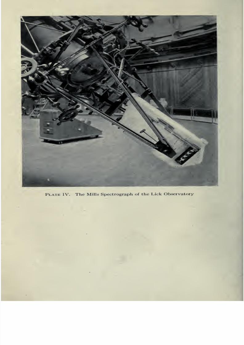
8/2/2019 The Binary Stars 1918
http://slidepdf.com/reader/full/the-binary-stars-1918 144/349
Plate IV. The Mills Spectrograph of the Lick Observatory

8/2/2019 The Binary Stars 1918
http://slidepdf.com/reader/full/the-binary-stars-1918 145/349
THE BINARY STARS II7
rigidity and temperature control of the spectrograph and to
improved methods of measuring and reducing the spectro-
grams.
In order to understand more clearly the manner in which
the optical and mechanical requirements are met in practice,
a detailed description will be given of a modern spectrograph
which was designed to have maximum efficiency for the par-
ticular problem of determining stellar radial velocities. Aview of the new Mills spectrograph attached to the thirty-six-
inch refractor of the Lick Observatory is presented in Plate
IV. The essential parts of this instrument are the same as
those described for the simple laboratory spectrograph;
namely, the slit, collimator lens, prism and camera lens,
except that here three 60° prisms of flint glass are employed.
The prisms, set at minimum deviation for 4500 A, produce a
deviation of this ray of 176°. A rectangular box constructed
of saw-steel plates, to which are connected respectively the
slit mechanism, the prism box, and the plate holder, by three
light steel castings, forms the main body of the spectrograph.
In the casting to which the prism box is attached are mounted
the collimator and camera lenses, both of which are achro-
matic for the region of 4500 A. The spectrograph has an
entirely new form of support, designed by Campbell, to in-
corporate the suggestion made by Wright, that such aninstrument should be supported near its two ends, like a biidge
truss or beam, in order to give minimum flexure. The support
is a frame work of T-bars extending down from the telescope,
the form and arrangement of which is such as to hold the in-
strument rigidly in the line of collimation of the large tele-
scope. The lower support is a bar passing through a rec-
tangular opening in the casting carrying the prism box. Thisbar is pivoted at the center of the casting and connected at
its two ends to the supporting frame. The upper support
consists of a cylindrical ring firmly attached to the frame
work. In this cylinder fits a spherical flange of the spectro-
graph casting, the two forming a universal joint. Any strains
originating in the supporting frame cannot, with this form of
mounting, be communicated to the spectrograph. Careful

8/2/2019 The Binary Stars 1918
http://slidepdf.com/reader/full/the-binary-stars-1918 146/349
Il8 THE BINARY STARS
tests of this instrument and of the spectrograph of the D. O.
Mills Expedition to Chile, which has the same form of mount-
ing, show that the effects of differential flexure have been
eliminated. This method of support permits, further, of a
very convenient mode of moving the spectrograph as a whole
in order to bring the slit into the focal plane of the large tele-
scope, since it is only necessary to provide sliding connections
on the frame, for the lower support.
Nearly all modern stellar spectrographs are provided with
reflecting slit plates inclined at a small angle to the collimation
axis, which enable the observer to view the star image directly
on the slit. This is accomplished through the aid of a total-
reflection prism, placed above the slit and outside of the cone
of rays from the telescope objective, which receives the light
from the slit and sends it to the guiding eyepiece. By placing
the slit parallel to the celestial equator, small errors of the
driving clock cause the star image to move along the slit,
which is desirable in order to obtain width of spectrum. Con-
stant and careful guiding is necessary to insure that the star's
image he kept exactly on the slit and that its motion along the
slit be such as to give a uniform exposure.
With a prism spectrograph and a straight slit the spectrum
lines are curved. The amount of the curvature depends upon
the optical constants of the instrument and the wave-length
of the line. This source of trouble in measuring the spectro-
grams may be eliminated for a short range of spectrum by
employing a slit of the proper curvatui^ to make the .spectrum
lines straight. Both three-prism instruments referred to above
are provided with curved slits.
As a source for the comparison spectrum, it is necessary to
select one giving a number of well-distributed lines in the part
of the spectrum to be studied. For example, for the new
Mills spectrograph in which the region 4400A to 4600A is
utilized, the spark spectrum of titanium is used. In the
southern instrument, arranged for the region 4200A-4500A,
the comparison source is the iron arc.
In order to eliminate the effects of any possible change in
the instrument during an exposure on the star, several impres-

8/2/2019 The Binary Stars 1918
http://slidepdf.com/reader/full/the-binary-stars-1918 147/349
THE BINARY STARS II9
sions of the comparison spectrum are made at regular inter-
vals. This is accomplished very conveniently and without
danger of changing the adjustment of the comparison appara-
tus by a simple device due to Wright. Two small total-reflec-
tion prisms are placed just above the slit, so that their adjoin-
ing edges define the length of the slit. Two light sources are
then so arranged that the beam of each is brought to a focus
on the slit by a small condensing lens after total reflection in
its respective prism.
The optical parts of the spectrograph should, of course, bemounted so that they cannot move, but care must be taken
that they are not cramped. This caution is especially perti-
nent with regard to the large prisms. In the Mills spectro-
graphs the prisms rest upon hard-rubber blocks and are
firmly clamped to one of the side plates of the prism box by
light steel springs which press against their upper surface.
Small hard-rubber stops prevent lateral motion of the prisms.
In order to prevent the effects of changing temperature, the
principal parts of the spectrograph are surrounded by a light
wooden box, tined with felt. Over the felt surface are strung
a number of turns of resistance wire. The regulation of the
heating current is effected by means of a very sensitive mer-
cury-in-glass thermostat by which the temperature inside of
the prism box is held constant during the night's work to
within a few hundredths of a degree Centigrade.
The function of the telescope objective, for observations of
stellar spectra, is that of a condensing lens and the brightness
of the point image in the focal plane is directly proportional to
the area of the lens and its transmission factor. If we had
perfect 'seeing' we should receive in the slit of the spectro-
graph, with the widths generally employed, about ninety per
cent, of the light in the star image. Due to atmospheric dis-
turbances the image of a star under average conditions of
seeing, is a circular 'tremor* disc whose diameter is four or
five times the width of the slit, so that the brightness of the
spectrum is not proportional to the area of the objective but
more nearly to its diameter. For example, the relative intensi-
ties of stellar spectra obtained with the same spectrograph

8/2/2019 The Binary Stars 1918
http://slidepdf.com/reader/full/the-binary-stars-1918 148/349
I20 THE BINARY STARS
respectively upon the thirty-six-inch and twelve-inch refrac-
tors of the Lick Observatory would be (allowing for the dif-
ference of transmission of the two), about astwo
to one, since,
for the photographic rays, the loss of light is for the former
about fifty per cent, and for the latter about twenty-five per
cent. When a visual refractor is used for spectroscopic work,
it is necessary to render it achromatic for the photographic
rays. This is accomplished for the thirty-six-inch refractor
by a correcting lens of 2.5 inches aperture placed one meter
inside the visual focus of the telescope. This lens introduces
an additional loss of light of fully ten per cent.
Since a silver-on-glass mirror has, under the best conditions,
a high reflecting power, and since it is also free from chromatic
aberration, it would seem that the reflector should be the more
efficient telescope to use in connection with a stellar spectro-
graph. The reflector, however, possesses its own disadvan-
tages, one of which is that it is very sensitive to changes of
temperature. Our experience with the thirty-six-inch refrac-
tor at Mount Hamilton and the thirty-seven and one-half
inch reflector in Chile, when used with high dispersion spec-
trographs, indicates that the relative light efficiency of the
two is about equal in the region of H7. For apertures up to
thirty-six inches one is inclined to favor the refractor for high
dispersion work, while for low dispersion, where considerable
extent of spectrum is desired, the reflector is, of course,
preferable.
The focal lengths of both refracting and reflecting telescopes
vary with change in temperature of the lens or mirror. It is,
therefore, necessary before beginning the night's work, and
with the reflector frequently during the night, to bring the
slit into the focal plane of the telescope, which as noted above,
is effected by moving the spectrograph as a whole in the line
of collimation of the instrument.
It is well known that all high dispersion spectrographs are
very wasteful of light, though to what extent is perhaps not
always appreciated. When stellar spectrographs of three-
prism dispersion are used in conjunction with large refractors
or reflectors the combined instrument delivers to the photo-

8/2/2019 The Binary Stars 1918
http://slidepdf.com/reader/full/the-binary-stars-1918 149/349
THE BINARY STARS 121
graphic plate probably less than two per cent, of the light
incident upon the telescope objective. Half of the light is
lost, as we have noted, before it reaches the slit. The remain-
ing losses occur at the slit, in the prisms and in the collimator
and camera lenses of the spectrograph. In order to avoid un-
necessary losses of light, the obvious conditions must be
satisfied, that the angular apertures of the collimator lens
and object glass are the same, and that the prisms and camera
lens are of sufficient aperture to admit the full beam from the
collimator. The most serious losses occur at the narrow slit
and in the prism train. Indeed, one of the most important
factors in the design of stellar spectrographs, for maximum
light efficiency, is the proper balancing of these two conflicting
elements, the transmission at the slit and the transmission of
the prisms. Thus, in the new Mills spectrograph, by using a
collimator of slightly greater focal length than the present
one (28.5 inches) with corresponding increase in aperture ofthe lens and prisms, a wider slit could be employed and still
maintain the present purity of spectrum. After allowance
is made for the increased absorption of the prism train, there
would remain a small gain in light transmitted. Although
theoretically possible, this gain would probably be more than
offset by the inferior definition of the larger prisms and the
added difficulty of eliminating flexure. It is necessary here,
as at so many points in the spectrograph, to sacrifice a little
in order to gain more elsewhere. In fact, the most efficient
design of spectrograph may be described as the one in which
the wisest compromises have been made between the various
conflicting interests.
The decision as to the resolution and dispersion to be em-
ployed is governed by several considerations : the type of stellar
spectrum to be studied, the size of the telescope at one's dis-
posal, and the brightness of the source whose spectrum can
be photographed with reasonable exposure times. With the
spectrograph here described two lines in the region of 4500Awhose wave-lengths differ 0.2 A are resolved, while the linear
dispersion for 4500A is I mm. = 11 A. In order to obtain
a spectrogram of suitable density of a star whose photographic

8/2/2019 The Binary Stars 1918
http://slidepdf.com/reader/full/the-binary-stars-1918 150/349
122 THE BINARY STARS
magnitude is 5.0, an exposure time of an hour and a half is
required. For stars of photographic magnitudes 6.0 to 6.5
the width of slit is increased, thus sacrificing to some degreethe purity of spectrum, but not enough to interfere seriously
with the accuracy of the measures. In the case of early type
stars whose spectra contain single lines, the question of reso-
lution is not important, and where these lines are also broad,
it is preferable to employ lower dispersion. The adjustments
of the various parts of the spectrograph call for continual
attention. It is necessary that the instrument be placedwith
its axis of collimation accurately in that of the large telescope
and frequent tests should be made to be sure that it remains
so. The comparison source must be adjusted so that its light
follows very nearly the same path as the star light in the spec-
trograph. Care must be exercised at every point in the pro-
cess of obtaining and measuring the spectrogram.
THE MEASUREMENT AND REDUCTION OF SPECTROGRAMS
For the measurement of spectrograms any one of the usual
forms of laboratory measuring microscopes will suffice. This
is merely a microscope on the stand of which is mounted a
carriage, movable by an accurate micrometer screw, in a
direction at right angles to that of the microscope axis.
In order to fix ideas, we shall assume that it is required to
measure and reduce the spectrogram of a2 Centauri, the posi-
tive of which is reproduced in Plate III. The spectrogram is
first clamped on the carriage of the microscope, and the usual
adjustments of focus and alignment of the plate are made.
Great care should be taken that the illumination of the field
of the microscope is uniform. Beginning with the comparison
line 4250 A, settings are made continuously along the plate on
good star lines and comparison lines as they chance to occur.
The plate is then reversed and the settings are repeated. It has
been shown by several investigators that the effects of errors
due to personal equation are practically eliminated by taking
the mean of the measures in the two positions. In the reversal
of the plate the spectrum is also inverted, which may so change
the appearance of the lines as to interfere with the elimination

8/2/2019 The Binary Stars 1918
http://slidepdf.com/reader/full/the-binary-stars-1918 151/349
THE BINARY STARS I23
of personal equation. Especially is this true if the lines are
curved. The effects of accidental errors in setting are reduced
by employing a number of lines.
The accompanying table contains the data of the measure
and reduction of this plate. Column I gives the wave-lengths
of the lines of the iron comparison and the normal wave-
lengths of the star lines, taken from Rowland's 'Preliminary
Table of Solar Wave-lengths'. In columns IV and V are
recorded respectively the settings on the comparison and star
lines (in revolutions of the micrometer screw). The displace-
ments of the iron lines in the star are evidently given directly
in amount and sign by the difference, star minus comparison
and these are entered at once in column VII (Displ.). Wecannot enter the displacements for the other star lines until
the normal positions of these lines have been obtained from
those of the iron comparison, by interpolation. This is effected
in the following manner:A smooth curve drawn by plotting, for the comparison lines,
the reading on each line and its corresponding wave-length,
respectively as ordinates and abscissae, will evidently repre-
sent for this spectrogram the relation existing between wave-
length and micrometer readings. From this curve—called a
'dispersion curve'—either the zero readings or the observed
wave-length of the stellar lines could be obtained. This curve
was found by Cornu and later by Hartmann to be nearly of
the form of an equilateral hyperbola so that it is approximately
represented by the equation
X — Xo = T- , (2)
A — Ao
where x is the micrometer reading on a line whose wave-length
is X and Xo, Xo, and c are constants. Since it is not practicable
to plot » the dispersion curve, the Cornu-Hartmann formula
furnishes a very convenient means of obtaining it. The values
of the three constants are determined from three equations
formed by substituting the micrometer readings and wave-
lengths of three lines, selected, one at each end of the region
of spectrum and the other near the middle. Micrometer read-

8/2/2019 The Binary Stars 1918
http://slidepdf.com/reader/full/the-binary-stars-1918 152/349
124
* 02 Centauri ft.
Date 191 1 Feb. 27
THE BINARY STARS
Plate No. 3791 III a 14^ 32.8'
X Table Co-Ta
Comp.4>
Stip'd D ispl rVs Vs
4250.287 54-886 54-886 54-758 — 128 319 —40.8
4250.945 55031 3 55-034 54-909 — 125 320 — 40.0
4282.565 61.819 13 61.832 61.710 — 122 335 -40.9
4283.169 61. 944 61.831 958
- 127 335 -42.5
4294.301 64 - 250 16 64.266 64. 140 - 126 338 — 42.6
4299.410 65-295 20 65-315 65.190 — 125 340 -42.5
4313- 034 68.039 67.944 061 - 117 349 -40.84313-797 68.190 68.090 212 - 122 349 — 42.6
4318.817 69.185 69.105 220 — 115 352 -40.5
4325- 152 70.431 70-355 469- 114 356 — 40.6
4325- 939 70.584 40 70.624 70.502 — 122 356 -43.4
4328.080 71.001 70.928 041 — 113 357 -40.3
4337.216 72.767 43 72.810 72.692 - 118 360 -42.5
4340.634 73.421 73.350 467- 117 362 -42.4
4359- 784 77.027 76.970 082 - 112 372 -41.7
4369.941 78.896 78.844 957 - 113 376 -42.5
4376.107 80.018 79.972 083 - III 378 — 42.0
4379 396 80.612 80.571 680 - 109 380 -41.4
4383.720 81.388 70 81.458 81.352 - 106 382 -40.5
4399 935 84-257 84.228 337- 109 390 -42.5
4404.927 85.126 86 85.212 85.105 — 107 392 -41.9
4406.810 85.453 85.432 539- 107 394 -42.2
4415- 293 86.913 93 87.006 86.898 — 108 397 -42.9
4425.608 88.664 88.662 759
-097 402 -39.0
4428.711 89.198 89.194 296 - 102 404 -41.2
4430.785 89-536 89-535 636 - lOI 404 -40.8
4435- 129 90.270 90.270 372- 102 406 -41.4
4435.851 90.380 90.378 482 - 104 406 -42.2
4442.510 91.482 108 91-590 91.491 - 099 411 -40.7
4443.976 91.724 91.732 831 - 099 412 -40.8
4447.892 92.365 92.375 473- 098 413 -40.5
4459-301 94.216 114 94-330 94-238 — 092 417 -38.4
4476.185 96.906 127 97 033 96.940 — 093 426 -39.6
4482. 379 97.872 131 98.003 97 905
- .098 428 -41.9
4494- 738 99.782 138 99.920 99 . 820 — .100 434 -43.4
35)1449.9
-4143
Scale= +0.13
va= +21.82
vd= — 0.07
Observed F —19.55 km.
8/2/2019 The Binary Stars 1918
http://slidepdf.com/reader/full/the-binary-stars-1918 153/349
THE BINARY STARS I25
ings of all other comparison and star lines are then computed
from the formula. The departure of this computed curve from
the true dispersion curve is furnished by a plot of the differ-
ences between the observed and calculated readings of the
comparison lines. The computed normal positions of the star
lines are then corrected for the difference between the com-
puted and observed dispersion curve. The decimal portions of
the results would be entered in column VI (Sup'd).^
As before, the difference, star line minus zero line, gives the
displacement in revolutions of the screw. In order to expressthis asAX, that is in units of wave-length, it is necessary to
know r, the number of angstrom units in one revolution of the
screw. The value of r for any point in the spectrum is evi-
dently the slope of the dispersion curve at that point, and is
equal to —- Finally, in accordance with the relation de-
duced earlier, v the observed radial velocity is obtained by
multiplying AX for each line by its corresponding factor
_ 299860
Each spectrogram may be reduced in the manner outlined
above, and some observers prefer to follow this method rigor-
ously for each stellar spectrogram. When this is done the
process is simplified by carrying through the computation in
wave-lengths, so that the displacement is expressed at once
in angstroms.
Since for the same spectrograph the form of the dispersion
curve differs but slightly for different temperatures, a simple
and practical method of reduction is offered by the following
procedure: A standard dispersion curve is computed once for
all, according to the method described above, from measures
of a solar spectrogram. With the aid of this all other spectro-
grams taken with the spectrograph may be quickly and easily
reduced. It is convenient to put this standard curve in
the form of a dispersion table in which are entered the
normal wave-lengths of the comparison and stellar lines used
2 The figures actually entered in this column in the example were obtained by a different
method of reduction which is explained in the paragraphs following.

8/2/2019 The Binary Stars 1918
http://slidepdf.com/reader/full/the-binary-stars-1918 154/349
126 THE BINARY STARS
for stars of different spectral classes, and the micrometer
readings corresponding to these wave-lengths. In this stan-
dard table are given also the values of rVs for each line.
Columns I and II and VIII, in the example, are taken from
such a table.
It is now only necessary to reduce the readings of the
standard table to the dispersion of the plate, by plotting the
differences between the observed and table readings; of the
comparison lines (recorded in Column III in the example).
From this curve the difference to be applied to the table read-
ing for each star line is read off. In the sixth column are given
the new table readings (for zero velocity) after this difference
has been applied. When there are comparison lines cor-
responding to star lines some observers follow rigorously the
process outlined, while others (as in the present example)
take the difference between the readings of the two as the
displacements. The last three columns contain, respectively,
the displacements (* minus Comp. or Sup'd), the factor rVs,
and the products of these two values, which are the relative radial
velocities of star and observer as supplied by the lines mea-
sured. The mean of the measures for forty lines gives as the
observed radial velocity —41.43 km. /sec. It will be noticed
that the dispersion of the star plate is about three-tenths of one
per cent, greater than that of the standard table, and conse-
quently the factor r (computed for the table) is too large, and
the numerical value of this velocity must be reduced by this
amount. This is allowed for, in the example, as scale correc-
tion. In practice, it is convenient to have several standard
tables corresponding to the dispersion of the spectrograph at
different temperatures. The one whose dispersion is nearest
that of the star plate is selected for use. Experience has
shown that the results obtained by the very simple methodjust described are of the same accuracy as those derived by
the longer process of computing a dispersion curve for each
plate.
If the spectrograph is not provided with a curved slit it is
necessary to introduce a correction for the curvature of the
lines. This correction may be computed from Ditscheiner's

8/2/2019 The Binary Stars 1918
http://slidepdf.com/reader/full/the-binary-stars-1918 155/349
THE BINARY STARS I27
formula^ or determined empirically from lines on a spectrogram
of the Sun, on the assumption that the curve of each line is a
parabola. The better method is to eliminate the source of
this correction by the use of a curved slit.
The observed radial velocity of a star is made up of the star's
velocity, V, with reference to the solar system, and the
velocity of the observer in the solar system. The latter con-
sists of three components, which arise from (one) the revolution
of the Earth around the Sun;
(two) the rotation of the Earth
on its axis; (three) the revolution of the Earth around the
center of mass of the Earth-Moon system. This last compo-
nent never exceeds ±0.014 km. /sec. and may be neglected.
The correction for the annual and diurnal motions of the
Earth are readily computed from the formulae given by
Campbell in Frost-Scheiner's Astronomical Spectroscopy
(pp- 338-345). The values for these in the example are given
respectively under Va and Vd. Hence, the observed radialvelocity of a2 Centauri with reference to the Sun on 191 1,
February 27.883 (Greenwich Mean Time) was— 19.55 km. / sec.
Methods of reduction which depend upon dispersion for-
mulae require an accurate knowledge of the wave-lengths of
the lines used in both the comparison and stellar spectra.
Accurate values of the absolute wave-lengths are not required
but their relative values must be well determined. For exam-
ple, a relative error of ±0.01A in the wave-length of any line
would produce an error in the velocity for that line of nearly .
a kilometer. Interferometer measures of the wave-lengths
in the spectra of a number of elements are now available, but
for the wave-lengths of solar lines it is still necessary to use
the determinations by Rowland. It has been shown that
errors exist in Rowland's tables, amounting in some cases to
as much as o.oi or 0.02A. Another and much more serious
difficulty arises, for stellar lines, from the fact that stellar
spectrographs have not sufficient resolution to separate lines
which were measured as separate lines by means of Rowland's
more powerful instrument. It is the practice of many obser-
• Cber die Kriimmung der Spectrallinien, Sitz. Ber. d. Math. Klasse d. k. Akad. Wien'
Bd. LI, Abth. II, 1865; also Frost-Scheiner, Astronomical Spectroscopy, p. 15, 1894.

8/2/2019 The Binary Stars 1918
http://slidepdf.com/reader/full/the-binary-stars-1918 156/349
128 THE BINARY STARS
vers, where two lines merge to form one line in the star spectrum,
to take the mean of the wave-lengths of the component lines,
weighted according to the intensities given by Rowland for
those lines in the Sun. Wave-lengths based on estimates of
intensity should naturally be regarded with suspicion, and in
fact we do not know, until the entire plate has been reduced,
whether we have chosen an erroneous wave-length or not.
It is well known that various stellar lines and blends behave
differently for stars of different types. The lines in solar type
starsare assumed to have the same wave-lengths as similar
lines in the Sun. In the case of stars of other spectral classes,
the solar lines which occur can be used in determining the
wave-lengths of the non-solar lines and blends. In this
manner special tables are constructed for stars of different
types.
When spectrographs of lower dispersion and resolution than
that of three prisms are employed for the measure of solar and
later-type spectra, the effect of uncertainties in wave-length
of the stellar lines, due to blends, becomes very serious. The
two methods of measurement and reduction which follow
eliminate the sources of error incident to the use of blends, and
erroneous wave-lengths as far as it is possible to do so. The
first is that due to Professor R. H. Curtiss and is called by him
the 'Velocity Standard Method'. In principle it amounts to a
determination of the wave-lengths of the lines in the spectrum
of a source whose radial velocity is known with the particular
spectrograph which is to be used for measures of stellar spectra
of this same class. Thus for the measures of spectra of the
solar type, a table similar to the one we have described above
is formed. The micrometer readings in this table, however,
are not computed from assumed wave-lengths, but are the
mean of the actual settings, on comparison and solar lines,
obtained on several spectrograms of the Sun. These standard
plates are produced as nearly as possible under the same con-
ditions as the stellar plates to be measured. The procedure in
the reduction of the measures by means of this table is then
the same as that described above. It is necessary, of course,
to correct the measured stellar velocity for the radial velocity

8/2/2019 The Binary Stars 1918
http://slidepdf.com/reader/full/the-binary-stars-1918 157/349
THE BINARY STARS 129
of the source when the standard spectrograms were taken.
Standard tables for the reduction of measures of stars of other
spectral classes may be formed in a similar manner, using as
the standard sources stars whose radial velocities are well
determined.
The second method is due to Professor Hartmann, and is in
principle the same as the preceding one, except that the star
plate is referred directly to the standard plate on a special
measuring microscope, known as the spectro-comparator.
The instrument is provided with two plate carriages, one of
which is movable. On one of the carriages the star plate is
placed and on the other, which is provided with a fine microm-
eter screw, is a standard plate of the Sun (taken with the
stellar spectrograph). The microscope has two objectives so
arranged that the images of portions of the two plates are
brought, by means of total reflection prisms and a reflecting
surface, to focus in the same plane and in the field of one eye-piece. By means of a silvered strip on the surface of one
prism, the central portion of the Sun's spectrum is cut out and
the star spectrum thrown into its place. In a similar manner,
central strips of the comparison spectra of the Sun plate are
replaced by those of the comparison spectra of the star plate.
An ingenious arrangement of the microscopes permits of
equalizing the scale of the two plates, by changing the relative
magnifying powers of the two objectives. The method of
measurement is, then, after proper alignment of the plates,
to bring corresponding sections of the two plates into the field
of the miscroscope, and by means of the micrometer screw
set the corresponding lines of the comparison spectra in the
same straight line. A setting is then made with the correspond-
ing lines of the solar and star spectra in the same straight line.
The difference between the micrometer readings in the two
positions is the displacement of the star lines relative to the
solar lines. In practice it is found sufficient to divide the
length of the spectrum into about fifteen sections, for each
of which these comparative settings are made. The mean of
the displacements, obtained with the plates in the direct and
reverse positions, when multiplied by the rVs for each section,

8/2/2019 The Binary Stars 1918
http://slidepdf.com/reader/full/the-binary-stars-1918 158/349
130 THE BINARY STARS
gives for each the value F*— Vq, where V* is the radial
velocity of the star and Vq that of the Sun. Theoretically,
the values of
V*— Vq should receive weights proportional
to
——in taking the mean. Although this correction is negligi-
ble, except where an extent of spectrum of 400 or 500A is
used, its introduction leads to a very simple method of com-
putation. Take the sum of the displacements in the direct
and reverse measures and multiply by a factor /= —. The
product is equal to the weighted mean of the values F*— Vq
for each section. This, corrected for the velocity of the original
Sun plate {Vq), gives the radial velocity of the star relative
to the observer. The reduction to the Sun is made in the
usual way. The factor / is a constant so long as the same
regions are used, and its values may be computed for all com-
binations of the regions that are used. The great advantage
of the method, aside from those which it possesses in common
with the velocity standard method, is that we are able to
measure and reduce in an hour a plate of a star rich in lines,
and practically utilize all the material on the plate. With the
older methods, to make such a comprehensive measure and
reduction, i.e., to utilize all of the lines on the plate, would
require one or two days.
For the measures of spectra of a type other than the solar
it is necessary to select for the standard plate a spectrogram
of a star of that particular spectral class. In order to obtain
the velocity for this standard spectrogram, it should be mea-
sured and reduced, either by the method first described or per-
haps preferably by the velocity-standard method. The
adopted value should be the mean of the measures made by
several different observers.
The spectro-comparator offers a very efficient method in
determining the differences in velocities of the same star, by
measuring a series of plates of the star with reference to one
of these selected as a standard.
Five of the six elements of a spectroscopic binary orbit
depend only upon the accurate determination of the relative

8/2/2019 The Binary Stars 1918
http://slidepdf.com/reader/full/the-binary-stars-1918 159/349
THE BINARY STARS I3I
radial velocities given by the series of spectrograms. One of
the most important applications of the Hartmann comparator
is, therefore, to the measurement of plates of a spectroscopic
binary.
For the measure and reduction of spectrograms of stars of
the earlier spectral classes, the use of the Cornu-Hartmann dis-
persion formula will suffice, inasmuch as the spectra of such
stars consist of lines due to the simple gases, the wave-lengths
of which have been accurately determined in the laboratory.
The measure and reduction of spectrograms of stars of the
solar and later classes of spectra are accomplished with great
saving of time and labor, and by a method free from some of
the uncertainties of wave-lengths, by the use of the spectro-
comparator. If the observer is not provided with such an
instrument the standard-velocity method is preferable to the
use of the dispersion formulae, at least until a system of
stellar wave-lengths of the requisite accuracy is available.To the reader who has followed the long and intricate process
of determining the radial velocity of a star, the question will
naturally occur, how do we know that the final result repre-
sents the star's velocity? Obviously, the final test of the
method is its ability to reproduce known velocities. Fortu-
nately, we have at hand a means of making such a test. Since
the orbital elements of the inner planets of the solar system
are well determined, we can readily compute the radial
velocity of one of these with reference to the Earth at any
given time. It is only necessary, then, to observe the relative
radial velocity of the planet and the Earth and compare this
with the computed value at the time of observation. At the
Lick Observatory spectrograms of Venus and of Mars are
secured at frequent intervals with the stellar spectrograph
and measured by the observers in the regular course of mea-
suring stellar plates. With the three-prism spectrograph, de-
scribed above, the observed and computed velocities of these
two planets generally agree to within =1=0.5 km., or the una-
voidable error of measure. When the spectrograms are
measured by several observers, the effects of personal equa-
tion are to some extent eliminated in the mean, and an agree-

8/2/2019 The Binary Stars 1918
http://slidepdf.com/reader/full/the-binary-stars-1918 160/349
132 THE BINARY STARS
ment within a few tenths of a kilometer is to be expected. Acontinual check is thus afforded on the adjustments of the
spectrograph and the measurement of the spectrograms.
REFERENCES
General
Campbell. Stellar Motions, Yale University Press, 1913.
Doppler's Principle
Kayser. Ilandbuch der Spectroskopie, Bd. 2.
Frost-Scheiner. Astronomical Spectroscopy, chapter 2, part II.
Instruments and Design
Campbell. The Mills Spectrograph. Astrophysical Journal, vol. 8,
p. 123, 1898.
Frost. The Bruce Spectrograph. Astrophysical Journal, vol. i^, p. i,
1902.
Hartmann. Remarks on the Construction and Adjustment of Spectro-
graphs. Astrophysical Journal, vol. 11, p. 400, 1900; and vol. 12,
p. 31, 1900.
Keeler. Elcmentar\' Principles Governing the Efficiency of Spectro-
graphs for Astronomical Purposes. Sidereal Messenger, vol. 10,
p. 433. 1891.
Newall. On the General Design of Spectrographs to be Attached to
Equatorials of Large Aperture, Considered Chiefly from the Point
of View of Tremor-discs. Monthly Notices, Royal Astronomical
Society, vol. 65, p. 608, 1905.
VOGEL. Description of the Spectrographs for the Great Refractor at
Potsdam. Astrophysical Journal, vol. 11, p. 393, 1900.
Wright. Description of the Instruments and Methods of the D. O.
Mills Expedition. Publications of the Lick Observatory, vol. g,
part 3, 25, 1905.
Methods of Measurement and Reduction
Campbell. The Reduction of Spectroscopic Observations of Motions
in the Line of Sight. Astronomy and Astrophysics, vol. 11, p. 319,
1892. Also Frost-Scheiner, Astronomical Spectroscopy, p. 338.

8/2/2019 The Binary Stars 1918
http://slidepdf.com/reader/full/the-binary-stars-1918 161/349
THE BINARY STARS 133
CuRTiss. A Proposed Method for the Measurement and Reduction of
Spectrogram for the Determination of the Radial Velocities of
Celestial Objects. Lick Observatory Bulletin, vol. j, p. 19, 1904;
Astrophysical Journal, vol. 20, p. 149, 1904.
Hartmann. tlber die Ausmessung und Reduction der Photographi-
schen Aufnahmen von Sternspectren. Astronomische Nachrichten,
vol. 755, p. 81, 1901.
. A simple Interpolation Formula for the Prismatic Spectrum.
Astrophysical Journal, vol. 8, p. 218, 1898.
-. The Spectro-comparator. Astrophysical Journal, vol. 24, p.
285, 1906. Publikationen des Astrophysikalischen Observatorium
zu Potsdam, vol. 18, p. 5, 1908.

8/2/2019 The Binary Stars 1918
http://slidepdf.com/reader/full/the-binary-stars-1918 162/349
CHAPTER VI
THE ORBIT OF A SPECTROSCOPIC BINARY STAR
The problem of determining the orbit of a binary system
from measures of radial velocity, made in the manner described
in the previous chapter, differs in several important particularsfrom that of computing an orbit from micrometric measures of
position angle and distance. It has been shown that microm-
eter measures provide the data from which the projection of
the orbit of the companion star with respect to its primary can
be drawn, the true relative orbit following, correct in propor-
tions but of unknown linear dimensions. The radial velocities,
on the other hand, when plotted against the times, produce a
periodic curve, having the general appearance of a distorted
sine-curve; from this curve we are to find the elements of the
true orbit of the star with respect to the center of gravity of
the system of which it forms one component.^
Figure 7 illustrates the conditions of the problem. Let the
XF-plane be tangent to the celestial sphere at the center of
motion, and let the Z-axis, perpendicular to the JsTF-plane, be
parallel to the line of sight along which the radial velocities
are measured. The velocities are considered positive (+) when
the star is recedingfrom, and negative ( — ) when it is approaching
the observer. The orientation of the X and F-axes remains
unknown. Let PSA be the true orbit of the star with respect
to the center of motion and let the orbit plane intersect the
ZF-plane in the line NN'.
Then, when the star is at any point S in its orbit, its distance
z from the X F-plane will be
z = rsmisin{v + co)
1 It is here assumed that the spectrum of only one component is visible; when both com-
ponents give spectra, we may determine the relative orbit of one with respect to the other,
using the same formulae but changing the value of the constant of attraction. The relative
and absolute orbits are, of course, similar in every respect.

8/2/2019 The Binary Stars 1918
http://slidepdf.com/reader/full/the-binary-stars-1918 163/349
THE BINARY STARS 135
the symbols in the right hand member of the equation having
the same significance as in the case of a visual binary star.
Figure 7
The spectrograph, however, does not give us the distances of
the star from the XF-plane, but the velocities of its approach
to, or recession from this plane, generally expressed in kilo-
meters per second. The radial velocity at point S is equal to
dzjdt, and is therefore expressed by
dz ...... dr^ . .
dv— = sin t sin {v -f- CO) 1- ^ sin ^ cosCij + co)
dt dt dt
From the known laws of motion in an ellipse we have
dv tia{i -\- ecosv) dr fxaesinv
dt V
and therefore
ii a sin i
dt Vi
dz
dt V][ecosco + COS (d + 0))] (i)
8/2/2019 The Binary Stars 1918
http://slidepdf.com/reader/full/the-binary-stars-1918 164/349
136 THE BINARY STARS
which is the fundamental equation connecting the radial veloci-
ties with the elements of the orbit.^
The observed velocities evidently contain the velocity, V,
of the center of mass of the system, which is a constant quan-
tity for any given simple binary system,^ as well as the variable
velocities due to the star's orbital motion and the quantity Vmust therefore be subtracted from the observed values to make
them purely periodic. In other words, the velocity curve is
purely periodic only with respect to a line representing the
velocity of the system as a whole. This line is called the
F-axis.
Equation (i) applies only to the velocities counted from the
F-axis. If d^ /dt represents the velocity as actually observed
(i.e., the velocity referred to the zero-axis) we shall have the
relation ^
dt dt
Methods of determining the position of the F-axis will be
given later; for the present we shall assume it to be known.
Five constants enter the right hand member of equation (i),
viz., a sin i, e, n, co and (through v) T. These express the five
orbit elements which it is possible to determine by measures
of radial velocity.
* In place of (» + co) the symbol m ( = the argument of the latitude) is often used, the
expressions for — and r— written
dt dt _dr f . , . , du f\/p / r .
/ \n— =x —^ e sin (u — (a), and r— = '..u:— = —__ [i -\- ecos(u — w) Jdt Vp dt r Vp
and hence the fundamental equation in the form
<*« / . w— = —=: sin » (cos u + e cos 00).
dt Vp
In these equations /> f= a (i — e)] is the semi-parameter of the true ellipse and /
denotes the constant of attraction, which, when the spectrum of only one component is
visible, and the motion is determined with reference to the center of mass of the system,
takes the form , k being the Gaussian constant; when both spectra are visible andm + mi
the motion of one star with respect to the other is determined, f = k v^m + mu It is clear
that the form of the fundamental equation will be the same whatever value we may assign
to'/ and the constant of attraction may therefore be disregarded until the question of the
relative masses in the system comes up for discussion.
3 In a triple or multiple system, this quantity will itself be variable.
* The symbol 7 is often used for the velocity of the system instead of V.

8/2/2019 The Binary Stars 1918
http://slidepdf.com/reader/full/the-binary-stars-1918 165/349
THE BINARY STARS 137
Since the inclination of the orbit plane is not determinable,
the value of a, the semi-major axis, must also remain unknown.
It is therefore customary to regard the function a sin i as an
element. Further, it is clear that the position of the line of
nodes cannot be determined though we can find the times when
the star passes through each of the nodal points. The various
elements have the same definitions as in the case of visual
binary star orbits (see page 72) except that the angle co in spec-
troscopic binary orbits is always measured from the ascending
node, the node at which the star is moving awayfrom the observer.
It will be seen later that the radial velocity has its maximum
positive value at this node and its minimum positive value (or
maximum negative value) at the descending node. It should
also be noted that the unit of time for // (and therefore for P)
is the day, not the year as in visual binary orbits.
Theoretically, values of the radial velocity at five different
times suffice for the complete solution of equation (i); prac-
tically, no computer undertakes an orbit until a considerable
number of measures is available which give the velocities at
short intervals throughout the entire revolution period. To
secure a satisfactory distribution of the observations a pre-
liminary value of the period is necessary and such a value can
ordinarily be obtained without difficulty by plotting the early
observations on coordinate paper, taking the times, expressedin Julian days and decimals of a day, as abscissae and the
velocities, expressed in kilometers per second, as ordinates. Aconvenient epoch as origin for the period is selected near the
beginning of the series, preferably one corresponding to a
point of maximum or minimum velocity. If later measures
indicate that the period is in error, a new period which is a
submultiple of the original one will often prove satisfactory.
In difficult cases, the following artifice may be found helpful.'^
Copy from one-third to one-half of the series of observed
points, choosing the time interval best covered by observa-
* This was suggested to me by Dr. R. K. Young who says that it has been used with
good results by several computers of binary star orbits at the Dominion Observatory. No
mention of the device has been found in print and its author is unknown to me. Its use-
fulness arises from the fact that, in effect, it doubles the number of observations for a given
time interval.

8/2/2019 The Binary Stars 1918
http://slidepdf.com/reader/full/the-binary-stars-1918 166/349
138 THE BINARY STARS
tion, on transparent paper; slide the copy along the original
plot, keeping the time-axis in coincidence, until some point
on the copy falls approximately upon a different point in the
original at which the velocity is changing in the same direction.
The time interval between the two points is evidently equal
to the period or a multiple of the period.
Schlesinger ^ has published a criterion that may be applied
to advantage in cases where an observer has accumulated
many plates of a star which apparently shows variable radial
velocity without being able to determine any period. It con-sists in constructing a frequency curve for the velocities by
"dividing the total range exhibited by the measured velocities
into successive groups of equal extent, say three kilometers
each, and then counting the number of velocities that fall
within these groups. Regarding these numbers as ordinates,
we plot them and join the ends by a smooth curve." This
curve is
comparedwith the well-known error-curve; if the
two are the same, within reasonable limits, we may conclude
that the differences in the measured velocities are due to
errors of observation, and afford no support for the assumption
that the star is a spectroscopic binary. If the two curves
differ, the star is a binary and the form of the frequency curve
will give an idea as to the general character of the orbit and
frequently furnish a clew to the period. For Schlesinger shows
that circular orbits, elliptic orbits with periastron at descending
node, elliptic orbits with periastron at ascending node, and
elliptic orbits with periastron removed 90° from the nodes, all
have characteristic frequency curves which differ in form from
the error-curve. When the nature of the frequency curve has
shown to which of these classes the orbit in question belongs,
it becomes very much easier to decide upon the epochs for the
various observed velocities, and thus upon an approximate
value for the period.
When the period is approximately known all of the observa-
tions may be reduced to a single revolution by subtracting
^ Astrophysical Journal, vol. 41, p. 162, 1915. In his paper on the "Orbit of the Spec-
troscopic Binary X Aurigae" (Journal R. A. S. C. vol. X, p. 358), Young shows that the
errors of measurement affect the expected distribution in such a manner as to mask to a
considerable degree the presence of the orbital variation.
8/2/2019 The Binary Stars 1918
http://slidepdf.com/reader/full/the-binary-stars-1918 167/349
THE BINARY STARS 139
multiples of the period from the later dates. A preliminary
curve is drawn to represent the plotted positions as closely as
possible. The deviations from the curve at points near the
mean of the maximum and minimum velocities, where a change
in the periodic time will have the greatest effect, will indicate
advisable changes in the assumed period and these are readily
found by dividing the deviations of such critical observations,
expressed in time, by the number of revolutions elapsed. Asecond curve is then drawn whose periodic time will generally
be very close to the true value. In practice it will frequentlyhappen that two or three measures of the radial velocity of a
star are available which were made (perhaps at another obser-
vatory) several years before the series of spectrograms for the
orbit computation is begun. When an approximate value of
the period has been found from the later series, these early
plates will determine its true value with high precision. Gen-
erallythey
arenot used
in findingthe other orbit elements.
When the period has been determined as accurately as
possible and a series of spectrograms has been accumulated
giving the velocities at points well distributed throughout the
entire period, the most probable curve is drawn, by estimation,
through the points as plotted, and, if the ingenious methods of
superposition devised by Schwarzschild and Zurhellen are to be
used, the curve should be prolonged through a revolution and
a half. The plotted points used for this curve should repre-
sent normal positions, formed by combining several velocities
observed at very nearly the same orbit phase, whenever the
number of observations is sufficient to permit such combina-
tions. In making the combinations, the question of weights
arises, and here the practice of computers varies considerably,
for several factors enter. The character of the lines on the
spectrograms, broad or narrow, sharp or ill-defined, strong or
weak, is one factor; the number of lines is another; if the
plates have been taken with different telescopes and spectro-
graphs, a third factor is introduced. These must all be con-
sidered in assigning the weights to each plate. The only direc-
tion that can be given is the general one to use rather a simple
system of weighting. It will rarely be of advantage to assign

8/2/2019 The Binary Stars 1918
http://slidepdf.com/reader/full/the-binary-stars-1918 168/349
140 THE BINARY STARS
fractional weights, or to use a range of weights greater than,
say, four units. The weights should, of course, be assigned to
each plate, at the time of measurement.The errors in drawing the most probable curve have con-
siderable effect upon the accuracy of the determination of the
elements. At best the curve is not likely to be a perfect repre-
sentation of the elliptic motion which caused it since it is
natural to bend the curve slightly in or out at different points
to satisfy the more or less exact observations. This difficulty
is inherent and for it thereis
apparently no remedy other thanthat of testing the first orbit by a trial ephemeris and making
the small changes in the elements which are indicated by the
residuals.^
If Figure 8 represents a velocity curve, it is evident from
equation (i) that the points A and B correspond respectively
to the ascending and descending nodes of the star's orbit, for
at the times of nodal passage we have(z;
-f co) =0°,
and(y + 0)) = 180°, respectively and therefore cos (z; + co) = =»= i.
The radial velocity thus reaches its maximum and minimum
values at the nodal points.
Taking A and B as the magnitudes of the curve-ordinates
at the points of maximum and minimum reckoned from the
F-axis, regarding 5 as a positive quantity and writing for
IJL a sin ibrevity K
V,we have
A =K{i -\- e cos co)
B = K{i — e cos co)
and therefore
A-{-B
2 KA-B
2
K e cos CO
A-Be cos CO
A+B
(2)
"> King's method affords a graphical test of the first orbit found, see page 154.

8/2/2019 The Binary Stars 1918
http://slidepdf.com/reader/full/the-binary-stars-1918 169/349
THE BINARY STARS 141
o lu
2 >

8/2/2019 The Binary Stars 1918
http://slidepdf.com/reader/full/the-binary-stars-1918 170/349
142 THE BINARY STARS
Hence we may write equation (i) in the form
— =K[e cos 0)
+cos(i'
+co)
J
=1 cos {v -\- co)
(3)at
22and (la) in the form
F H 1 cos (y + co) = FiH cos (z^+cu). (3a)ft/ 2 2 2
i<L is therefore the half-amplitude of the velocity curve.
Up to the point now reached practically all methods of spec-
troscopic orbit determination are identical.
But when thefundamental relations are given as above, and the curve has
been drawn, quite a variety of methods is available for com-
puting the orbit elements, other than the period, which is
assumed to be known.
Of these, the method devised by Lehmann-Filhes will first
be presented, essentially in full; other methods will then be
treated in less detail. The student who desires to study the
various methods more fully is referred to the important papers
given in the references at the end of the chapter.
METHOD OF LEHMANN-FILHES
Given the observations, and the velocity curve drawn with
the value of P assumed as known, the first step is to fix the
F-axis, the line defining the velocity of the center of gravity
of the system. This is found by the condition that the integral
of dz jdt, that is, the area of the velocity curve, must be equal
for the portions of the curve above and below the F-axis. By
far the easiest method of performing this integration is to use
a planimeter. A fine, approximately correct, is first drawn by
estimation; the areas contained between it and the curve
above and below are measured, and the difference between
the two is taken. The position of the axis is then shifted to
eliminate this difference, and the measures are repeated. It
will rarely be necessary to make more than one correction to
secure an accurate value of the position of the F-axis, which,
by this method, depends upon the entire curve.
If a planimeter is not available, the areas above and below
the axis may be equalized by using coordinate paper for the

8/2/2019 The Binary Stars 1918
http://slidepdf.com/reader/full/the-binary-stars-1918 171/349
THE BINARY STARS 143
plot of the curve and counting the small squares in each area.
Approximate mechanical integration, as advised by Lehmann-
Filhes, may also be resorted to, by those who enjoy this form
of recreation.
Having found the F-axis, the ordinates to it are next drawn
from the points of maximum and minimum velocity, A and B.
It is at this point, as Curtis says, that the method is weakest,
for slight errors in fixing the position of A and B may easily
arise. It is well to apply the check afforded by the requirement
that area AaC (Figure 8) must equal CbB and DaA equal BbD.Since C and D lie on the F-axis the velocities at these points
dzare zero, hence from equations (3) and (2) we have for -—
at
at these points
COS (v + o)) = = — e cos CO (4)A-{-B
If Vi is the true anomaly corresponding to the point C, whichis traversed by the star on the way from the ascending to the
descending node, and V2y the true anomaly for the point D,
sin (vi + co) will be positive, sin (v2 + co) negative, and we
shall have
cos {Vi + Co) = —-—, COS {V2 + CO) = -
A+ B A-\-B
,n(., + co)= ___,sm(.. + co) = -^-p^
(5)
Let Zi and Z2 denote the areas ^ AaC and bBD (Figure 8)
respectively, and let ri and ^2 be the radii vectores for the
points C and D.
Then
Zi = ri sin i sin {vi + co)
Z2 = r2 sin i sin (1^2 + co) = — r2 sin i sin (f 1 + o))
and therefore
Zi n i+ecost;2 ,^.
(6)
Z2 r2 i+^cosi'i
8 These areas represent the distances of the star from the XF-plane at the points in its
orbit corresponding to {vi + co) and (wj + co).

8/2/2019 The Binary Stars 1918
http://slidepdf.com/reader/full/the-binary-stars-1918 172/349
144 THE BINARY STARS
since r = . Write (v -\- co — co) for v, in (6), expand,i+ ecost;
and reduce, with the aid of the relations in (5) and (4), andwe have
Zi sin {vi + co) — e sin CO
Z2 sin (t^i -f- w) + e sin CO
whence
Z2+Z1. ,
, , 2^/AB Z2-\-Zi . .
e sin CO = sin {vi + co) = . (7)
Z2-Z1 ^ ^ ^ A +B Z2-Z,'^'
Equations (7) and the last of (2) determine e and co. The
values of A and B are taken from the curve, and the areas Zi
and Z2 are quickly integrated from the curve portions AaC
and bBD by means of a planimeter, the latter area being
regarded as negative in sign. Since the areas enter as a ratio,
the unit of area used is entirely immaterial.
At the time of periastron passage v = o°\ hence from equa-
tion (3) we have
— =X(i 4-e)cosco (8)
dtp
which gives the ordinate corresponding to the point of peri-
astron passage. Two points of the curve will have the same
ordinate, but since (v + co) equals 0°, 180°, and 360° for the
points A, B, and Ai, respectively, there will be no ambiguity
as to the position of the periastron point. The abscissa of
this point, properly combined with the epoch chosen for the
beginning of the curve, defines T, the time of periastron pas-
sage. Instead of using (8) we may find T by determining Efor the point C for which the value of v is known, and then
employ the formulae
\i+ l
^tan K V
t-
e
E — esmE(8a)
or, if the eccentricity is less than 0.77, M may be taken directly
from the Allegheny Tables, and T found from the relation
M = yL{t-T). (8b)

8/2/2019 The Binary Stars 1918
http://slidepdf.com/reader/full/the-binary-stars-1918 173/349
THE BINARY STARS I45
Such procedure is especially advisable when the periastron
point falls near points ^4 or 5 on the curve.
By definition (page 140) we have
fjL a sin i
K. =
Vi-
and hence
AVi-e2 A-\-B Vi -
a Sim 2 a sin t
from which we may find the value of the product a sin i.
Since the unit of time for A and B is the second, while for /x
it is the day, the factor 86,400 must be introduced. Our
equation then becomes
Ka sin i = 86,400— V i -V = [4.i3833]ii:P Vi - e^ (9)
the number in brackets being the logarithm of the quotient
86400 -^ 2 TT.
Summarizing, the practical procedure is:
1. Find the period as accurately as possible by successive trials and
plot the most probable velocity curve on the basis of normal places.
2. Find the position of the F-axis by integration of areas, using the
planimeter, if available.
3. Measure the ordinates for points A and B and find the areas of
AaC and bBD expressed in any convenient units.
4. From (2) and (7) determine K, e, and w.
5. From (8), or by calculation from the value of v, for the point C,
determine T.
6. From (9) determine a sin i.
To test the elements by comparison with the observations,we compute the radial velocity for each date by the formulae
M = flit - T) = E - esinE
-Vi?an J/^ V =./-;—!— tan ^2 E
— = V -\- Ke cos CO -\- K cos {v -\- co)
dt
(10)

8/2/2019 The Binary Stars 1918
http://slidepdf.com/reader/full/the-binary-stars-1918 174/349
146 THE BINARY STARS
The value of v for each value of M may be taken directly from
the Allegheny Tables, if e is less than 0.77.
To illustrate Lehmann-Filhes's methodI
have chosen theorbit computed for k Velorum, by H. D. Curtis, the velocity
curve for which is given in Figure 8.
The observations used were as follows:
Julian Day. G.M.T. Vel. Julian Day, G. M. T. Vel.
2416546.739 + 68.5km 2417686.591 + 33.8kni
60.703 + 12.9 91.572 + 38.2
97651 + 65.7 92.545 + 43-2
6912.601 + 53.3 96.480 + 46.7
7587.844 + 58.6 7701.494 + 52.7
88.788 + 57.9 41.466 + 22.1
90.829 + 58.5 46.463 + 0.3
91.824 + 64.8 49.470 - 7.6
97.788 + 65.8 50.479 - 8.8
7609.790 4- 62.0 51.463 - 13.3
54.534 — 21.0 53.457 - 19.2
55.556 - 19.2 58.451 — 29.0
58.570 - 15.2 59.460 — 24.6
59.545 - 14.5
The small circles representing the first four observations,
which are important in determining the period, owing to their
distance in time from the later ones, are barred in the diagram.
The period, P, was assumed to be 116.65 days, and the begin-
ning of the curve is at Julian day 2416476.0. This is not
exactly at a minimum, as may be seen from the diagram.
From measures of the curve we find
A = 46.3 Zi = AaC = H- 0.168
B = 46.9 Z2 = bBD = - 0.259
A -]- B = 93.2 Z2 + Zi = — 0.091
A — B = — 0.6 Z2 — Zi = — 0.427
K = {A-\- B)l2 = 46.6

8/2/2019 The Binary Stars 1918
http://slidepdf.com/reader/full/the-binary-stars-1918 175/349
THE BINARY STARS 147
The solution of equations (2), (7), (8) then proceeds as
follows
log
log 2 0.3010 log (I + e) 0.0828
log Vab 1.6684 /oj COS CO 8.48oon
colog {A + B) 8.0306 logic 1.6684
log (Z2 + Zi) 8.956on
o.3696n\^^i
^' A o.23i2n
colog (Z2 — Zi) ^^Q^dtp/
log e sin co 9.3286 ordinate p -- 1.7 km
log (A - B) 9.7782n .*. from curve tp = 98.4
( =) e cos CO 7.8o88n
\A-\-B )7^ = J. D. 2416457.75
log tan CO i.5i98n log const. 4.1383
CO 91.73° logic 1.6684
sin CO 9.9998 logP 2.0669
/.k^ Vi - e" 9.9902
loge 9.3288 log a sin i 7.8638
e 0.21 a sin i 73,000,000 + kni
The preliminary values thus obtained are next tested by
comparing the velocities derived from them by equations (10)
with the observed velocities. To illustrate, let us compute the
velocity for J. D. 24164^6.0, twenty days after the origin
adopted in our curve. We have
/ = 2416496.0 log cos {v -f co) 9.8277n
/- r = + 38.0 logic 1.6684
it-T) 1.57978 1.496in
log/x 0.48942A+B . .
,cos(t'+ co)
2
- 31.3 km
M 117.27°A-B
2
-0.3
V 136.01 V + 20.7
f + CO 227.74d^
dt
= — 10.9 km
» r is here taken one revolution earlier than the date for the periastron point marked
on the curve. Using equation (8a), or (8b) we obtain T = J. D. 2416458.0 which is
adopted.

8/2/2019 The Binary Stars 1918
http://slidepdf.com/reader/full/the-binary-stars-1918 176/349
148 THE BINARY STARS
In this mannerwe compute as many velocities as necessary to
obtain a curve for comparison with the observed velocity curve.
In the present instance this was done for every tenth day, andthe results plotted as heavy black dots in the figure. By noting
the discrepancies, it appears that the branch on the apastron
side of the computed curve, if drawn, would be a little too
sloping, the other branch too steep, which indicates that the
computed value of e is a little too large. Changing this ele-
ment and making the corresponding slight changes required
in T andco,
the test was repeated, and after a few trials, thefollowing elements were adopted as best representing the ob-
servations :
V = -\- 21.9km
P = 116.65 days
e = 0.19
K = 46.5
0) = 96.23°
r =J. D. 2416459.0
a sin i = 73,000,000km
The correction to the value of V was found last of all from
the residuals of the final ephemeris by the simple formula
[v] .
^^, where n is the number of observations and v the residual,
n
o — c. The residuals from the final ephemeris and the final
curve may be found in Lick Observatory Bulletin, No. 122, 1907.
Lehmann-Filhes's method may be termed the classical one,
and it is probably more generally used than any other. The
method proposed by Rambaut is considerably longer and
more involved than the later ones, and for that reason will not
be described here. Wilsing's method, as originally published,
was suitable only for orbits of small eccentricity, but Russell
later extended it to make it applicable to larger eccentricities
as well. This method is purely analytical, consisting in finding
a Fourier's series for the velocity in terms of the elements. It
should be very useful in special cases, particularly when the
period is so nearly a year that one part of the velocity curve
is not represented by any observations; but it is considerably
8/2/2019 The Binary Stars 1918
http://slidepdf.com/reader/full/the-binary-stars-1918 177/349
THE BINARY STARS 149
longer, in time consumed, than the method of Lehmann-Filh^s
and other geometrical methods to be described presently, and
it will not be further considered here.
Certain features of the methods proposed by Schwarzschild
and Zurhellen are both ingenious and practical. The following
account of them is taken in substance from Curtis's article
already referred to.
schwarzschild'S METHOD
Given the velocity curve and the period, Schwarzschild first
determines the time of periastron passage. Let Mi and M2 be
the observed velocities {i.e.j the velocities measured from the
zero-axis) of maximum and minimum, and draw the line whose
ordinate is —^-
^. This line is the mean axis. Mark upon2
it the points corresponding to P 12 and 3P J2 ; then lay a piece
of semi-transparent paper over the plot, copy upon it the curve
together with the mean axis and mark also the points o, P I2,
P, and 3P/2. Shift the copy bodily along the mean axis for
the distance P/2, and then rotate it 180° about this axis,—i.e.,
turn the copy face downward on the original curve keeping
the mean axis in coincidence and bring the point o or P of the
copy over the point P/2 of the original. The curves will then
cut each other in at least four points, and, in general, in four
points only. These will fall into two pairs, the points of each
pair separated by an abscissa interval P/2. The points of one
pair will be on different branches of the velocity curve, and it
is easy to see that, if Vi and V2 represent their true anomalies,
we shall have V2 = Vi -\- 180°. Now the only two points in the
true orbit which are separated by one-half a revolution and for
which at the same time this relation of the true anomaliesholds are the points of periastron and apastron passage.
Hence, to select these points, choose the two points of inter-
section of the curve and its copy which are separated by half
a revolution and which lie on different branches of the curve.
To distinguish periastron from apastron we have the criteria:
First, at periastron the velocity curve is steeper with respect
to the axis than at apastron ; Second, the curve is for a shorter

8/2/2019 The Binary Stars 1918
http://slidepdf.com/reader/full/the-binary-stars-1918 178/349
150 THE BINARY STARS
time on that side of the mean axis on which the point of peri-
astron lies.
This method is exceedingly good except when the eccen-
tricity is small. In this case co and T are quite indeterminate
and small errors in drawing the velocity-curve will be very
troublesome. The method of Lehmann-Filhes is then to be
preferred.
Having the value of T, the value of co is next found as fol-
lows: From equations (la) and (3) it is readily seen that the
position of the mean axis is
= V -\- K e COS w = Fi2
and that, accordingly, the ordinate 2' of any point measured
from the mean axis is
z' = ^- Vi = Kcos(v-{- oj). (II)
dt
Now at periastron v = 0°, at apastron v = 180°. Hence, if
we call the ordinates from the mean axis for these, points z'p
and z'o we shall have
z'p ^p — z'aCOS CO = ^ or cos w = -^
(12)
K 2K
from which to determine co. This method is at its best when
CO is near 90°.
Zurhellen has simplified Schwarzschild's method of finding
e, and we shall give this simpler form in connection with Zur-
hellen's simple method of finding co.
zurhellen's methods
Zurhellen's method of determining co depends upon the rela-
tions between the velocities for the two orbit points whose
true anomalies are i 90°. From equation (11) we have, when
V = - 90°,
2i = + iC sin CO
and when v = -\- 90°,
Zi= — K sin CO.

8/2/2019 The Binary Stars 1918
http://slidepdf.com/reader/full/the-binary-stars-1918 179/349
THE BINARY STARS 151
Moreover, for these two points we have
£1 = — £2
Ml = - ikf2
(t,-T)= -{t2-T)',
hence the two points are symmetrically placed with respect
to the mean axis in the F-coordinate and with respect to the
point of periastron passage in the -AT-coordinate. They may
therefore be determined by rotating the curve copy through
180° about the intersection of the ordinate of periastron with
the mean axis, and noting the two points of intersection of the
copy with the original curve. If the curve is prolonged through
one and one-half revolutions, another point 180° from one of
these, say at + 270°, can be determined in similar manner
and the location of all three can then be checked by drawing
the lines connecting the point z; = + 270° with v = — 90°,
and V = — 90° with v = -\- 90°. These lines should cut the
mean axis at its intersections with the ordinates of periastronand apastron respectively. From the ordinates of the two
points V = =±=90°, measured from the mean axis, we have
si — 22 ^ 21—22 , .
sin CO = , or tan w = (12)
2K Zp — Za
from which to find w. The method is at its best when co is small.
Zurhellen's simplification of Schwarzschild's method of find-
ing e is also based upon the relations between the two points
V = ^ 90°. Since
tan 3^ £ = tan >^ i; tan (45° - H <t>)
where(f>
is the eccentric angle, we have, when v = ±90^
£1 = - (90° - 0), £2 = + (90° - ct>).
Similarly,
IT /'^^o , •, , sin sin (90° - 0)Ml = — (90° -- 0) + -
»o
o ^ ^ sin (^ sin (90° — </>)
sin I
sin (h s
M2 = + (90° -<i>)-sin I
and therefore
M. - M. = 3^ 0. - <.) = (:8o° -2.t>)-"" ^"°°
V^^ . (.3)Sin I

8/2/2019 The Binary Stars 1918
http://slidepdf.com/reader/full/the-binary-stars-1918 180/349
152 THE BINARY STARS
The value of {h — /i) may be read off directly from the dia-
gram, and the value of (90° — 4>) can then be taken from the
table for equation(13),
computed by Schwarzschild, which is
given below. Like the above method for finding co this method
is best when co is small.
Schwarzschild' s Table for the Equation
360'2 7;
— sin 2 r; = {t2 - ti).
t2
—tx t2
—ti t2
—tl
VP
VP
VP
0° 0.0000 30°. 0290 60° 0.1956
I 0.0000 31 0.0318 61 . 2040
2 . 0000 32 . 0348 62 0.2125
3 . 0000 33 . 0380 63 0.2213
4 O.OOOI 34 0.0414 64 0.2303
5 O.OOOI 35 . 0450 65 0.2393
6 .
0002 36.
0488 66 0.2485
7 0.0004 37 0.0527 67 0.2578
8 . 0006 38 . 0568 68 0.2673
9 0.0008 39 0.061 69 0.2769
10 O.OOII 40 . 0656 70 0.2867
II 0.0015 41 0.0703 71 0.2966
12 . 0020 42 0.0751 72 0.3065
13 0.0025 43 . 0802 73 0.3166
14 0.0031 44 0.0855 74 0.3268
15 . 0038 45 0.0910 75 0.3371
16 0.0046 46 . 0967 76 0.3475
17 . 0055 47 0.1025 77 0.3581
18 . 0065 48 0.1085 78 0.3687
19 0.0077 49 O.II47 79 0.3793
20 0.0089 50 O.I2I2 80 0.3900
21 0.0103 51 0.1278 81 . 4008
22 0.0II7 52 0.1346 82 0.4II7
23 0.0133 53 O.I416 83 0.422624 0.0I5I 54 0.1488 84 0.4335
25 0.0170 55 O.I56I 85 0.4446
26 0.0I9I 56 0.1636 86 0.4557
27 0.0213 57 O.I713 87 . 4667
28 0.0237 58 0.1792 88 0.4778
29 . 0262 59 0.1873 89 0.4889
30 . 0290 60 0.1956 90 . 5000

8/2/2019 The Binary Stars 1918
http://slidepdf.com/reader/full/the-binary-stars-1918 181/349
THE BINARY STARS 153
Zurhellen also gives a method for finding the eccentricity
by drawing the tangents to the curve at the points of perias-
tron. These can be drawn quite accurately except when the
periastron falls near a maximum or a minimum of the curve.
Slight changes in its position will then introduce considerable
changes in the inclinations of the tangent lines:
The expression for the slope of a tangent may be written
dx 2 IT dx _ 2 IT I dx
~dt~ ~F
' dM~ P ' i-ecos£* dE
where ^ (= ~r ) represents the ordinate drawn to the F-axis.
Also, by introducing the known values
cos E — sin <}) . cos <^ sin £cos V = , sin z;
=I — e cos E I —e cos E
andtransforming and simplifying
we maywrite the funda-
mental equation (3) in the form
dz __ , cos<f>
cos CO cos £ — sin oj sin EX = — = K cos <p .
•
dt I — e cos E
Differentiating with respect to E, substituting and reducing,
we have
dx 2 TT
^,.— cos
(f>
cos CO sin £ — sin co cos £+
^ sin co , .
— =—Kcos<t>. —. (14)
dt P (i — ecosEY
At periastron E = 0° and at apastron E = 180°, whence we
have
dx — 2 TT K COS sin CO dx _ -\- 2 w K cos(f)
sin co
dtp P{i - eY' dta P (i + eY
and therefore
dxIdx (i + eY
dtpI
dta (i - eY
whence
9 + »
«'.

8/2/2019 The Binary Stars 1918
http://slidepdf.com/reader/full/the-binary-stars-1918 182/349
154 THE BINARY STARS
king's method
The methods of orbit computation so far described in this
chapter all rest upon the curve drawn to represent as closely
as possible the observed velocities and, at the same time, to
satisfy the conditions for elliptic motion. Unless the measures
are very precise, the first approximation will ordinarily not be
satisfactory. As stated on page 140, the only remedy is to
compute an ephemeris from the elements and, on the basis of
the residuals thus found, to draw a new curve. This process
is sometimes repeated three or four times before a curve is
found which will yield elements upon which a least squares
solution may be based.
The method devised by Dr. King, which is now to be pre-
siented, aims to substitute a rapid graphical process for testing
the preliminary curve. Dr. King shows that a circle having
its center on the mean axis and a radius equal to K, the semi-
amplitudeof the velocity curve,
"may beused as the equiv-
alent of the hodograph of observed velocities."^°
Let the velocity curve and the circle be drawn (see Figure 9)
and the abscissa distance corresponding to one revolution (P
being assumed to be known) be divided into any convenient
number of parts, say forty. ^^ Now mark consecutive points
on the circumference of the circle by drawing lines parallel to
the mean axis at the intersections of the velocity curve with
the ordinates corresponding to successive values of the ab-
scissa and extending them to the circle. The circumference
will be divided into forty unequal parts, but these inequalities
will be found to vary uniformly. "The points will be close
together in the vicinity of one point of the circle, and will
gradually separate as we proceed in either direction therefrom,
until at the diametrically opposite point they reach their maxi-
mum distance apart." These unequal arcs of the circle cor-
respond to the increase in the true anomalies in the orbit in
the equal time intervals, and therefore the point of widest
10 For the proof of this relation the reader is referred to the original article, Astrophysical
Journal, vol. 27, p. 125, 1908.
11 An even number should be chosen, and it is obviously most convenient to make the
drawing upon coordinate paper.

8/2/2019 The Binary Stars 1918
http://slidepdf.com/reader/full/the-binary-stars-1918 183/349
THE BINARY STARS 155
s
I ^s
^
^ %
i "i\
%h
n.?A^ nI
\^
Xt
h \
s \
:s21
iS?Fpr-
Figure 9. King's Orbit Method. Graph for « = 0.75, w = 60°

8/2/2019 The Binary Stars 1918
http://slidepdf.com/reader/full/the-binary-stars-1918 184/349
156 THE BINARY STARS
separation of the circle divisions corresponds to periastron,
that of least separation, to apastron. Further, the angle be-
tween the F-axis and the periastron-half of the diameterbetween these two points is equal to co. To locate the point of
periastron on the velocity curve, find the intersection of the
steeper branch of the curve with a line drawn from the peri-
astron point on the circle parallel to the mean axis.
It is evident that the division points of the circumference
will be symmetrically disposed with respect to the apsidal
diameter(the diameter joining periastron and apastron points)
only when one of the division points in the line of abscissae
corresponds to an apse. In general, the periastron point will
lie within the longest division of the circumference, the apas-
tron point within the shortest. If desired, the approximate
position of one of these points may be used as a new origin
from which to set off the fortieths of the period along the axis
of abscissae, and two division points on the circle may then be
brought into closer coincidence with the apsidal points.
Since —- varies inversely as the square of the distance fromat
the focus, by measuring the lengths di and d2 of the arcs at
points where v equals Vi and V2, we have
di _ {i -\- e cos viY
di{i -\- e
cos^2)^
and hence if the arcs are measured at the points of periastron
and apastron where v respectively equals 0° and 180°,
d2 \i - ej
V di— V d2
V di-^ V~d,
or e = = • (16)
which determines e.
It is generally sufficiently accurate to measure the chords
instead of the arcs; when the eccentricity is high and the arcs
at periastron inconveniently long, additional points of division
may readily be inserted.
It will be observed that this process furnishes a more thorough test
of the accuracy of the graph (velocity curve) than the method of
equality of areas. If it is imperfect, the points on the circumference

8/2/2019 The Binary Stars 1918
http://slidepdf.com/reader/full/the-binary-stars-1918 185/349
THE BINARY STARS I57
of the circle will not be distributed according to the regular order of
increase or decrease of the included arcs. If an ordinate of the graph
is too long or too short, the corresponding point on the circumfer-ence will be too near to or too far from the vertical diameter. If the
points of maximum and minimum velocity have not been well deter-
mined, the diameter of the circle will be too long or too short. In the
former case all the points of the circumference will be crowded away
from the vertical diameter; in the latter, toward it.^^
To test a given set of elements by comparison with the ob-
servations proceed as follows
Construct a circular protractor on some semi-transparent
material (e.g., celluloid or linen tracing cloth) and divide it
into forty parts by radii to points on the circumference repre-
senting the true anomalies for the given value of e correspond-
ing to every 9° of mean anomaly {i.e., to fortieths of the period).
If the eccentricity is less than 0.77 the values of the true anom-
aly can be taken directly from the Allegheny Tables.On the plot of the orbit draw a circle of radius K with its
center on the mean axis and draw its vertical diameter. Set
the protractor upon the circle, making the centers coincide,
and turn the apsidal diameter of the protractor until it makes
an angle equal to co with the vertical diameter. Now note the
points where the radial lines representing the anomalies inter-
sect the circumference of the circle. The abscissa axis of the
plot also having been divided into forty equal parts, erect
perpendiculars at the points of division equal to the corres-
ponding ordinates of the circle. A freehand curve through the
extremities of these perpendiculars (i.e., ordinates to the mean
axis) gives the computed curve or 'ephemeris', and the resid-
uals can be read directly from the plot. The advantage of
using coordinate paper will be obvious.
From the account just given it will appear that King's
method is longer, or at least not shorter, than the others de-
scribed if only a single orbit is to be computed. But when
orbit computation is to be taken up as a part of a regular pro-
gram of work, the method has very decided advantages. It
is then to be used as follows:
12 King, loc. cit.

8/2/2019 The Binary Stars 1918
http://slidepdf.com/reader/full/the-binary-stars-1918 186/349
158 THE BINARY STARS
Let a set of protractors be constructed on transparent cellu-
loid with radii representing the divisions in true anomaly for
every 9° of mean anomaly for the values e = 0.00, e = 0.05
to g = 0.95.
With the aid of these protractors draw curves on tracing
linen representing orbits with all values of e from 0.00 to 0.95
and all values of co from 0° to 360°. The intervals for e should
be 0.05, save for the larger values which are seldom used, and
for CO, 15°. Practically, values of w to 90° will suflfice, the curves
for the values in the remaining quadrants being obtained by
inverting the sheet, and by looking through the linen from the
back in the two positions. Given the protractors, a complete
set of curves may be constructed in about ten hours' time.
Having such a set of curves, plot the normal places for any
given binary star on the same scale as these curves in time and
in velocityP Now place the standard curves upon the plot
until one is found that fits the observations. "If two or more
curves seem to give about equally good representations, it is
quite possible to interpolate elements between the graphs
plotted."1*
By this process values of e correct to within one or two
hundredths and of co correct within a few degrees can generally
be obtained at the first trial and with an expenditure of less
than ten minutes' time. The time of periastron passage fol-
lows at once, and this set of preliminary elements may then
be used as the basis for a least squares adjustment. The pro-
cedure has been found very satisfactory at the Dominion
Observatory at Ottawa.
Russell's short method
Professor Henry Norris Russell has devised a graphical
method which is equally simple in its practical application.^^
" Since the velocity curve is ordinarily based on from fifteen to twenty normal places
the work of multiplying by the appropriate reduction factors will require a very few minutes
only. Of course the amplitude of the curve as well as the period must be known before
the reduction factors can be obtained. These are known with sufficient accuracy from the
preliminary plots.
" R. K. Young. Orbit of the Spectroscopic Binary 2 Sagittae. Journal R. A. S.C., vol.
17, p. 131. 1917.
^* Aslrophysical Journal, vol. 40, p. 282, 1914.

8/2/2019 The Binary Stars 1918
http://slidepdf.com/reader/full/the-binary-stars-1918 187/349
THE BINARY STARS I59
Write equation (la) in the form
dz
P = F + -— = F+X e cos CO + ^ cos (v + w) =G + i^ cos (v + co)
^'(17)
where p represents the observed radial velocity.
Then {G + K) is the maximum, (G — K) the minimum
value of the velocity so that G and K may be estimated at
once from the freehand curve. The period is also assumed
to be known. Equation (17) may then be written in the form
P-Gcos {v + co) (18)
and the value of (v + co) computed for each observed value of p.
If we subtract the corresponding values oi M -\- Mo from each of
these, we shall have values of {v — M) -\- {oj — Mo). The second part
of this expression is constant, while the first is the equation of the
center in the elliptic motion. During a revolution this varies between
equal positive and negative limits which depend only on the eccen-
tricity, and are nearly proportional to it, as is shown in the following
table.
Eccentricity O.IO 0.20 0.30 0.40 0.50 0.60 0.70 0.80 0.90
Maximum
equation
of center ii°.5 23°.o 34°.8 46°.8 S9°.2 72^3 86°.4 loa^.s I22°.2
If the values of v — M -{- a — Mo are plotted against those of
M -i- Mo, we obtain a diagram which, since it represents the relations
between the mean and the true anomalies, we may call the anomaly
diagram. If on this diagram a curve is drawn to represent the plotted
points, half the difference between its maximum and minimum ordi-
nates will be the greatest value of the equation of the center, from which
e may be found at once by means of the table. The mean of the maxi-
mum and minimum ordinates will be the value of w — Mo. The
instants when v — M -\- oi — Mo has this value are those of periastron
and apastron passage, the former corresponding to the ascending branch
of the curve, which is always the steeper. The abscissae of the corres-
ponding points of the curve are Mo and Mo + 180°. The values of e.
Mo, and co are now known, and the remaining elements may be found
at once from K and G.

8/2/2019 The Binary Stars 1918
http://slidepdf.com/reader/full/the-binary-stars-1918 188/349
l60 THE BINARY STARS
According to Russell the "principal advantage of this method
is that the form of the curves which give v — M sls Si function
of M depends upon e alone." For further details and an illus-
trative example we refer the reader to the original memoir. Upto the present time the method has not come into general use.
A similar remark applies to the graphic method proposed
by Dr. K. Laves, in 1907, and, of course, to the two short
methods quite recently proposed by Dr. F. Henroteau, which
take advantage of the Allegheny Tables of Anomalies in a
novel way. References to the original papers containing thesemethods are given at the end of this chapter.
DIFFERENTIAL CORRECTIONS TO THE ELEMENTS
Whatever method may be used in finding the preliminary
orbit it is generally advisable to determine the correction to the
elements by the method of least squares.^^ The formula derived
by Lehmann-Filhes from which the coefficients for the observa-tion equations are to be computed may be written as follows:
d — = d V -{ [cos {v -\- 03) -\- e cos co]d Kdt
sin(i'+ co)sinr
f-K [cos CO {2 -\- e cos v)\ a e
I — e^
— K [sin {v -^ 0)) -\- e sin 03] dc^
-\- sin {v -\- co) {i -\- e cos vY ,1 ^ I'
(i - e2)''
- sin (t; -f o)) (I -f e cos v^,,,
{i - T)d ix . (19)(i — e)
'^
"^^ Publication Allegheny Observatory, vol. i, p. 33, 1908.
The advantages of applying the method of least squares to the definitive solution of
spectroscopic binary stars have been clearly stated by Schlesinger in this paper. "The
problem," he says, "involves the evaluation of five quantities (six if the period be included)
that are so interwoven as to make their separate determination a matter of some difficulty.
Herein lies the chief advantage for this case of the method of least squares; for it enablesus to vary all of the unknowns simultaneously instead of one or two at a time. .
Further, the method of least squares not only has the advantage of greater accuracy and
of telling us how reliable our results are, but it eliminates from the computations any
personal bias or arbitrary step . . . the method should be used in almost every case
where the elements are not avowedly provisional." Not all computers are so enthusiastic
as to the method. Judgment must of course be exercised in all orbit work as to whether
the data at hand warrant anything beyond the computation of purely provisional elements.
In spectroscopic binary orbits, for example, such factors, among others, as the number and
quality of the plates and their distribution over the velocity curve, the character of the
star's spectrum, and the character of the orbit must be considered in making this decision.

8/2/2019 The Binary Stars 1918
http://slidepdf.com/reader/full/the-binary-stars-1918 189/349
THE BINARY STARS l6l
In practice the period is almost always assumed to be known
with accuracy and the last term of the equation is omitted.
To facilitate the computation Schlesinger has transformed
this equation as follows:
Put
a = 0.452 sin V {2 -\- e cos v)
{i -\- e cos vYp =
(I + cY
T = d V -\- e cos ixi d K-\-
K cos w d e — K e swujj d 03
K = dK
TT = — K do)
zr2-21 ,
€ = — K deI - e^
\ I
- c
T = /fyL, J-LX£. J!-iTe I — e
ni= - K J-tl . ^L dfi, and u = {v + co).
\ I — e i — e
Then the equations of condition take the form
d^d — = r + cos u ' K -\- sinu- tt + a sin « • €
^^+ ^ sinu- T-\- ^ sin u- {t- T)m. (20)
The quantities a and /8 can be tabulated once for all and such
a tabulation is given by Schlesinger {loc. cit,) so arranged "as
to render the normal equations homogeneous and to enable all
multiplications to be made with Crelle's tables without inter-
polation." If this notation is used, the computer should have
these tables at hand.^^
When both spectra are visible on the plates, the orbitsfor
the two components with respect to the center of mass may be
determined separately. It is obvious that the two sets of
values of F, e, T, and P must be identical, the values of w
must differ by 180°, while the two values for K depend upon
" Dr. R. H. Curtiss has shown that this formula and therefore the least squares solu-
tion can be made appreciably shorter. (Publications Astronomical Observatory, University
of Michigan, Vol. II, p. 178, 1916).

8/2/2019 The Binary Stars 1918
http://slidepdf.com/reader/full/the-binary-stars-1918 190/349
l62 THE BINARY STARS
the relative masses of the components. The preliminary ele-
ments for the two components, when independently deter-
mined, will, in general, not harmonize perfectly. To obtain
the definitive values the best procedure is the one first sug-
gested, I believe, by Dr. King.^^ It consists in combining all
the observations, those for the secondary with those for the
primary, into a single set of observation equations (equations
of condition) and solving for one complete set of elements. If
we write co' = (co + i8o°) and distinguish the values of K for
the two components by writing Ki and K2 respectively, theequations in the notation of (19) assume the form
d— = dV -\- [cos(r+ co) -f- e cosco]Jivi+ [cos(f + co')+ ecosco'j dKidi
n sin (v + 03) sin v Jj^
-h \ cosco {2 -\- e cos v) \ K\
LI i-^'J
f ,sin(t;+a)')sinT;
n 1 1^ 1 j
+\ cos CO (2
+e cos ij) \ KiXde
—I I
sin (r + co) + e sin CO \ K\-]r \ sin (r + co') + ^ sin co' \ KAdw
+ sin (t» + co) (i 4- ^ cos vY Ki
1 M+ sin {v + co') (I + e cos v)^ K^ —-^^ ,^^
d T, (21)
the value of the period being assumed to require no correction.
Since K2 does not affect the residuals of the primary com-
ponent, nor Ki those of the secondary, the terms dK^ and dKi
disappear from the equations representing the residuals from
the primary and secondary curves, respectively.
SECONDARY OSCILLATIONS
When the orbit of a spectroscopic binary star has been com-
puted and the theoretical velocity curve drawn, it is some-
times found that the observed normal places are so distributed
i«See Harper's paper, in Publications of the Dominion Observatory, Vol. i, p. 327. I9i4-
Dr. Paddock independently developed an equivalent equation. Lick Observatory Bulletin,
Vol. 8, pp. 156, IS7. 1915-

8/2/2019 The Binary Stars 1918
http://slidepdf.com/reader/full/the-binary-stars-1918 191/349
THE BINARY STARS 163
with respect to the curve representing simple elliptic motion
as to suggest that a secondary oscillation is superimposed upon
it. The question is whether this grouping arises from some
source of error in the measurement of the spectrograms, from
erroneous values of one or more of the orbit elements, or from
a real oscillation such as might be produced, for example, by
the presence of a third body in the system. This question has
been discussed by Schlesinger and Zurhellen, and later by
Paddock. Schlesinger and his associates at the Allegheny
Observatory have shown that 'the blend eflfect' caused by the
overlapping of the absorption lines of the two component
:_^^i-i'^%
*i^ -(ST'
-it s
"E ^^-^.^^'
:
^^5^^^Figure 10. Radial Velocity Curve of f Geminorum. The secondary oscillation
is probably real
Spectra "may produce such an apparent oscillation." They
have also shown that it may be produced by chance errors in
the velocities derived from the different lines of the spectrum,
and they are convinced that a critical analysis of the data will
dispose of a considerable percentage of cases wherein secondary
oscillations have been suspected. The possibility of a real
secondary oscillation must of course be recognized, and when
a full analysis has shown that such an oscillation is present,
additional terms may be introduced into the equations of con-
dition to represent it upon the assumption that it is produced
by a third
bodyrevolving in
acircular orbit about one of the
other two components. In the cases that have arisen thus
far this simple assumption has yielded a satisfactory represen-
tation of the data, though it is apparent that there is no
reason for limiting such additional bodies to circular orbits.
Let T' represent the time when the secondary curve crosses
the primary from below, K' the semi-amplitude of the sec-
ondary oscillation, m' the ratio of the principal period to that

8/2/2019 The Binary Stars 1918
http://slidepdf.com/reader/full/the-binary-stars-1918 192/349
l64 THE BINARY STARS
of the secondary oscillation, assumed to be known (it is gen-
erally taken to be an integer), and put u' = m'li {t — T'),
T = — m' jjlK' dT',K' = dK^; then the additional terms re-
quired in equation (20) are
+ sin u' • k' -\- cos u' ' t' . (22)
For a more complete discussion of secondary oscillations the
reader is referred to the articles cited above.
ORBITS WITH SMALL ECCENTRICITY
In a circular orbit the elements T and w obviously have no
significance, and when the eccentricity is very small they
become practically indeterminate by the geometrical or graph-
ical methods which have here been described. Further, if
approximate values are assumed, it is impossible to find cor-
rections to both elements from the same least squares solutionbecause the coefficients for the differential corrections will be
nearly or quite equal. Some computers have overcome this
difficulty by assuming the preliminary value of cu as final, and
determining corrections to 7", but this is hardly a solution of
the problem. In such orbits the analytic method possesses
great advantages, as has been shown by several investigators,
notably Wilsing and Russell, Zurhellen, and Plummer. Pad-
dock has quite recently examined the question in great detail,
extending some of the earlier developments and adapting them
for computation. A full account of these methods would re-
quire more space than is available here, and it has seemed best
to refer the reader to the original papers.
REFERENCES
The following list of papers relating to one phase or another
of the computation of orbits of spectroscopic binary stars, while
not exhaustive, contains most of the important ones.
Rambaut, a. a. On the Determination of Double Star Orbits from
Spectroscopic Observations of the Velocity in the Line of Sight.
Monthly Notices, Royal Astronomical Society, vol. S^^ P- 3 16, 1891.
8/2/2019 The Binary Stars 1918
http://slidepdf.com/reader/full/the-binary-stars-1918 193/349
THE BINARY STARS 165
WiLSiNG, J. tJber die Bestimmung von Bahnelementen enger Doppel-
sterne aus spectroskopischen Messungen der Geschwindigkeits-
Componenten. Astronomische Nachrichten, vol. 134, p. 90, 1893.
Lehmann-Filhes, R. Cber die Bestimmung einer Doppelsternbahn
aus spectroskopischen Messungen der in Visionradius liegenden
Geschwindigkeits-Componente. Astronomische Nachrichten, vol.
136, p. 17, 1894.
ScHWARZSCHiLD, K. Ein Verfahren der Bahnbestimmung bei spec-
troskopischen Doppelsternen. Astronomische Nachrichten, vol. 752,
p. 65, 1900.
Russell, H. N. An Improved Method of Calculating the Orbit of a
Spectroscopic Binary. Astrophysical Journal, vol. i^, p. 252, 1902.
. A Short Method for Determining the Orbit of a Spectroscopic
Binary. Astrophysical Journal, vol. 40, p.. 282, 19 14.
NijLAND, A. N. Zur Bahnbestimmung von spektroskopischen Dop-
pelsternen. Astronomische Nachrichten, vol. 161, p. 105, 1903.
Laves, K. A Graphic Determination of the Elements of the Orbits of
Spectroscopic Binaries. Astrophysical Journal, vol. 26, p. 164, 1907.
Zurhellen, W. Der spectroskopische Doppelstern Leonis. Astro-
nomische Nachrichten, vol. 1^3, p. 353, 1907.
. Bemerkungen zur Bahnbestimmung spektroskopischer Dop-
pelsterne. Astronomische Nachrichten, vol. 775, p. 245, 1907.
. Weitere Bemerkungen zur Bahnbestimmung spektroskopi-
scher Doppelsterne u. s. w. Astronomische Nachrichten, vol. 177,
p. 321, 1908.
. Uber sekondare Wellen in den Geschwindigkeits-Kurven
spectroskopischer Doppelsterne. Astronomische Nachrichten, vol.
187, p. 433, 191 1.
King, W. F. Determination of the Orbits of Spectroscopic Binaries.
Astrophysical Journal, vol. 27, p. 125, 1908.
Curtis, H. D. Methods of Determining the Orbits of Spectroscopic
Binaries. Publications A.S.P., vol. 20, p. 133, 1908. (This paper
has, with the author's permission, been very freely used in preparing
my chapter on the subject.)
Plummer, H. C. Notes on the Determination of the Orbits of Spectro-
scopic Binaries. Astrophysical Journal, vol. 28, p. 212, 1908.
8/2/2019 The Binary Stars 1918
http://slidepdf.com/reader/full/the-binary-stars-1918 194/349
l66 THE BINARY STARS
ScHLESlNGER, F. The Determination of the Orbit of a Spectroscopic
Binary by the Method of Least Squares. Publications of the Alle-
gheny Observatory, vol. i, p. 33, 1908.
. On the Presence of a Secondary Oscillation in the Orbit of
30 H Ursae Majoris. Publications of the Allegheny Observatory, vol. 2,
p. 139, 191 1.
. A Criterion for Spectroscopic Binaries, etc. Astrophysical
Journal, vol. 41, p. 162, 1915.
Paddock, G. F. Spectroscopic Orbit Formulae for Single and Double
Spectra and Small Eccentricity. Lick Observatory Bulletin, vol. 8,
p. 153, 1915.
CuRTiss, R. H. Method of Determining Elements of Spectroscopic
Binaries. Publications of the Astronomical Observatory, University
of Michigan, vol. 2, p. 178, 1916.
Henroteau, F. Two Short Methods for Computing the Orbit of a
Spectroscopic Binary Star by Using the Allegheny Tables of
Anomalies. Publications A. S. P., vol. 2Q, p. 195, 191 7.
8/2/2019 The Binary Stars 1918
http://slidepdf.com/reader/full/the-binary-stars-1918 195/349
CHAPTER VII
ECLIPSING BINARY STARS
We have seen that one of the first binary systems to be dis-
covered with the spectrograph was Algol (jS Persei), long known
as a variable star. There are other stars whose light varies in
the same peculiar manner as that of Algol; that is, while it
remains sensibly constant at full brightness the greater part
of the time, at regular intervals it fades more or less rapidly
to a certain minimum. It may remain constant at this mini-
mum for a short time and then recover full brightness, or the
change may be continuous. In either case the entire cycle of
change is completed in a small fraction of the time of constantlight between the successive minima.
The hypothesis that in every such case the star, as viewed
from the Earth, undergoes a total, annular, or partial eclipse,
the eclipsing body being a relatively dark star revolving with
the other about a common center of gravity, completely ac-
counts for the observed facts and has been proved to be
correct not only in the one instance, Algol, but also in that of
every Algol-type variable which has been investigated with
the spectrograph. Undoubtedly it is the correct explanation
for all stars of this type; they are all binary systems.
Unless the darker star is absolutely non-luminous, there
should be a second minimum when the bright star passes
between it and the Earth, the relative depth of the two minima
depending upon the relative intensity of the light of the two
stars and upon their relative areas. Such a secondary mini-
mum has been observed in jS Lyrae and in this star the light
is not quite constant at any phase, either maximum or min-
imum. There is now no doubt but that this star and others
like it are also binary systems.
It was formerly thought that a distinction could be drawn
between variable stars of the type of Algol and those of the

8/2/2019 The Binary Stars 1918
http://slidepdf.com/reader/full/the-binary-stars-1918 196/349
l68 THE BINARY STARS
type of /3 Lyrae, but measures with sensitive modern photo-
meters, such as the selenium-cell, the photo-electric cell, and
the sliding-prism polarizing photometers, and measures ofextra-focal images on photographic plates have attained such
a degree of accuracy that a variation considerably less than
one-tenth of a magnitude can be detected with certainty; and
it now appears that Algol itself not only has a slight secondary
minimum but that its light is not quite constant at maximum.
The distinction, therefore, breaks down and we may regard
all the stars of these two types as members of a single class,
calling them eclipsing binaries or eclipsing variables according
to the point of view from which we take up their investigation.
There are, in all, more than 150 eclipsing binary stars known
at the present time and a large percentage of them are too
faint to photograph with our present spectrographic equip-
ment. It is therefore a matter of great interest to inquire what
information, if any, as to the orbits of these systems can be
derived from their light curves, the curves, that is, which are
constructed by taking the observed stellar magnitudes as
ordinates and the corresponding times as abscissae.
Professor E. C. Pickering ^ made an investigation of the
orbit of Algol on the basis of its light curve as early as 1880,
and showed that a solution of such orbits was possible if certain
reasonable assumptions—for example, that the two stars are
spherical with uniformly illuminated disks and move in cir-
cular orbits—were granted. The subject was resumed by him
later, and was taken up also by Harting, Tisserand, A. W.
Roberts, and others. But the most complete investigation so
far is that begun at Princeton University, in 191 2, by Russell
and Shapley, the theoretical part being contributed, mainly,
by the former, the application to particular systems, mainly,
by the latter. The present chapter will be based entirely upon
this investigation.
In the most generaJi, case the problem is an extremely com-
plicated one, for the orbits must be regarded as elliptical with
planes inclined at a greater or less angle to the line of sight,
1 Dimensions of the Fixed Stars, with special reference to Binaries and variables of
the Algol Type. Proceedings American Academy of Arts and Sciences, vol. i6, p. i, 1881.

8/2/2019 The Binary Stars 1918
http://slidepdf.com/reader/full/the-binary-stars-1918 197/349
THE BINARY STARS 169
and the two components as ellipsoids, the longest diameter of
each being directed toward the other star. Moreover, the
disks may or may not be uniformly illuminated ; they may bedarker toward the limb, as our own Sun is, the degree of dark-
ening depending upon the depth and the composition of the
enveloping atmosphere, and the side of each which receives
the radiation from the other may be brighter than the opposite
side. The complete specification of an eclipsing binary system
therefore requires a knowledge of at least thirteen quantities,
which in Russell's notation, are as follows:
Orbital Elements Eclipse Elements
Semi-major axis a Radius of larger star r\
Eccentricity e Radius of smaller star r
Longitude of periastron Oi Light of larger star Li
Inclination i Light of smaller star L2
Period P and at least 3 constants defining
Epoch of principal conjunction to the amount of elongation, of dark-
ening at the limb, and of brighten-
ing of one star by the radiation of
the other.
The longitude of the node must remain unknown, as there is no hope
of telescopic separation of any eclipsing pair.
The value of a in absolute units can be found only from spectroscopic
data. In the absence of these, it is desirable to take a as an unknown
but definite unit of length, and express all other linear dimensions in
terms of it. Similarly, the absolute values of L\ and L2 can be deter-
mined only if the parallax of the system is known. But in all cases the
combined light of the pair, Li + L2, can be taken as the unit of light
and the apparent brightness at any time expressed in terms of this.
This leaves the problem with eleven unknown quantities to be deter-
mined from the photometric measures. Of these, the period is invari-
ably known with a degree of accuracy greatly surpassing that attainable
for any of the other elements, and the epoch of principal minimumcan
be determined, almost independently of the other elements, by inspec-
tion of the light-curve. Of the remaining elements, the constants
expressing ellipticity and 'reflection' may be derived from the observed
brightness between eclipses. These effects are often so small as to be
detected only by the most refined observations. The question of
darkening toward the limb may well be set aside until the problem is
solved for the case of stars which appear as uniformly illuminated disks.

8/2/2019 The Binary Stars 1918
http://slidepdf.com/reader/full/the-binary-stars-1918 198/349
170 THE BINARY STARS
This leaves us with six unknowns. Fortunately, systems of such
short period as the majority of eclipsing variables have usually nearly
circular orbits (as is shown both by spectroscopic data and by the
position of the secondary minimum). The assumption of a circular
orbit is therefore usually a good approximation to the facts, and often
requires no subsequent modification.
Russell's papers discuss first the simplified problem:
Two spherical stars, appearing as uniformly illuminated disks, and re-
volving aboul their common center of gravity in circular orbits, mutually eclipse
one another. It is required to find the relative dimensions and brightness of
the two stars, and the inclination of the orbit, from the observed light-curve.
Even in this form four different cases are presented, de-
pending upon the character of the photometric data and the
completeness of the observations; only one minimum or both
minima may have been adequately observed, and these may
or may not show a constant phase. To illustrate the method
ofinvestigation, I shall here present
(bypermission,
almostentirely in Russell's own words) the two simplest cases, namely,
those in which a constant phase has been observed in one or
both minima and in which the eclipses are therefore either
total or annular, and shall refer the reader who wishes to
pursue the subject to the original memoirs.
We may assume P and to as already known. If the radius of the rela-
tive orbit is taken as the unit of length, and the combined light of the
two stars as the unit of light, we have to determine four unknown
quantities. Of the various possible sets of unknowns, we will select
the following:
Radius of the larger star nRatio of radii of the two stars k
Light of the larger star Li
Inclination of the orbit i
The radius of the smaller star is then r2 = kri, and its light, L2 = i — Li.
It should be noticed that, with the above definitions, k can never exceed
unity, but L2 will exceed Li whenever the smaller star is the brighter
(which seems to be the fact in the majority of observed cases).
We will suppose that we have at our disposal a well-determined
'light-curve', or more accurately, magnitude-curve. . . . From

8/2/2019 The Binary Stars 1918
http://slidepdf.com/reader/full/the-binary-stars-1918 199/349
THE BINARY STARS 171
this we can pass at once to the intensity-curve, giving the actual light-
intensity / as a function of the time, by means of the equation
log/ = o.4(wo — w), (i)
where Wo is the magnitude during the intervals of constant light be-
tween eclipses (which is determined with relatively great weight by
the observations during these periods and, like P, may be found once
for all before beginning the real solution). This of course expresses / in
terms of our chosen unit Li + Li.
Such a magnitude-curve or intensity-curve will in general show two
depressions, or 'minima', corresponding to the mutual eclipses of thetwo components. Under the assumed conditions, it is well known:
1. That the two minima will be symmetrical about their middle points'
and that these will be separated by exactly half the period.
2. If the eclipse is total or annular, there will be a constant phase at
minimum during which the magnitude- or intensity-curve is horizontal;
but if the eclipse is only partial, this will not be the case.
3. The two minima will be of equal duration, but usually of unequal
depth. At anygiven phase during one minimum one of the stars will
eclipse a certain area of the apparent disk of the other. Exactly half a
period later, at the corresponding phase during the other minimum, the
geometrical relations of the two projected disks will be the same, except
that now the second star is in front, and eclipses an equal area—though
not an equal proportion—of the disk of the first. The intensity-curves for
the two minima must therefore differ from one another only as regards
their vertical scales, which will be in the ratio of the surface intensities of
the two stars.
4. The deeper (primary) minimum corresponds to the eclipse of the star
which has the greater surface intensity by the other. Whether this is the
larger or smaller star must be determined by further investigation.
Suppose that at any time during the eclipse of the smaller star by
the larger the fraction a of its area is hidden. The light received from
the system at this moment will be given by the equation
/i= I - aLz. (2)
Half a period later, an equal area of the surface of the larger disk, and
hence the fraction k'^o. of its whole area will be eclipsed. The observed
light will then be
l2= \- k^aLi. (3)
Since Li -f L2 = i, we find at once from these equations
(I - k) + ^-?-^ = a. (4)

8/2/2019 The Binary Stars 1918
http://slidepdf.com/reader/full/the-binary-stars-1918 200/349
172 THE BINARY STARS
If both minima have been observed and show constant phases, the
eclipse of the smaller star by the larger is total and the other eclipse
annular; in both cases an area equal to the whole area of the smaller
star is obscured; that is, a = i. If Xi and X2 are the values of the ob-
served intensities during the constant phase at the two minima, we
have by (4)
*' = '-^- (5)
Moreover, by (2), Xi = i — L2 = Li. The brightness of the two stars
and the ratio of their radii, are thus determined, leaving only ri and i
to be found.
There are, however, two solutions with different values of k accord-
ing as we regard the principal or secondary minimum as total. Weshall see later how we may distinguish the correct solution in a given
instance.
[In case only the primary minimum has been observed], if the ob-
served minimum intensity is X and we assume that the observed eclipse
is total, we have from (2), L2 = I — X; if annular, (3) gives k'^Li =
I — X. In either case, for any other value / of the observed intensity,
a = ^' (6)I—
We thus know a as a function of the time, and from this have to deter-
mine k, ri, and i.
Take the center of the larger star as origin, and let 6 be the true
longitude of the smaller star in its orbit, measured from inferior con-
junction. Then ^
e=^{t-to). (8)
From the light-curve and (6) we can find the value of a for any value
of 0y or vice versa. Now a, which is the fraction of the area of the
smaller disk which is eclipsed at any time, depends on the radii of the
two disks, and the apparent distance of their centers, but only on the
ratios of these quantities (being unaffected by increasing all three in
the same proportion). If 5 is the apparent distance of centers, we have
therefore
-'{^ry-i'-v)
2 For convenience, I have preserved the equation numbers as given in Russell's original
paper. His equation (7) is omitted because it does not relate to the cases here discussed.

8/2/2019 The Binary Stars 1918
http://slidepdf.com/reader/full/the-binary-stars-1918 201/349
THE BINARY STARS 173
where/ is a function, the details of calculation of which will be discussed
later.
For any given value of k we may invert this function,and write
b= (^, a). (9)
This function, or some equivalent one, may be tabulated once for all
for suitable intervals of k and a.
By the geometry of the system, we have
52 = sin2 Q _j_ cos^ i cos2 e = cos^ i + sin^ i sin" d, (10)
whencecos" i + sin" i sin" 6 = ri" {^(/^.a)}". (11)
Now let ai, a^, as be any definite values of a and Bu 62, Oz the cor-
responding values of 6 (which may be found from the light-curve).
Subtracting the corresponding equations of the form (11) in pairs, and
dividing one of the resulting equations by the other, we find
sin" di - sin" 62 = [<i> (k, ai) }"- {0 (ife.aa)}^
f^
f7- = \f/(k, 01, a2, 03). (12)
sin" 02 - sin" ds = {<t> {k, az) }"- {</. (k, aa) }'
The first member of this equation contains only known quantities.
The second, if ai, a2, and as are predetermined, is a function of k alone.
If this function is tabulated, the value of k in any given case can be
found by interpolation, or graphically. The equations (11) can then
be used to find ri and i.
A theoretical light-curve may then be found, which passes through
any three desired points on each branch of the observed curve (assumed
symmetrical). These points may be chosen at will by altering the
values of ai, a2, and as. In practice it is convenient to keep az and as
fixed, so that\J/becomes a function of k and ai only, and may be tabu-
lated for suitable intervals in these two arguments. This has been
done in Table II, in which a2 is taken as 0.6 and as as 0.9. If ^ = sin^ $2,
B = sin^ 02 — sin^ 63, (12) may be written
sin" di = A-^ B^p(k, ai). (13)
The points a and b on the light-curve corresponding to a2 and as, to-
gether with the point corresponding to any one of the tabular values
of ai, then give a determination of k. By taking a suitably weighted
mean of these values of k, a theoretical light-curve can be obtained
which passes through the points a and b, and as close as possible to the
others. By slight changes in the assumed positions of a and b {i.e., in
the corresponding values of 6, or of / — to), it is possible with little

8/2/2019 The Binary Stars 1918
http://slidepdf.com/reader/full/the-binary-stars-1918 202/349
174 THE BINARY STARS
labor to obtain a theoretical curve which fits the whole course of the
observed curve almost as well as one determined by least squares. The
criterion of this is that the parts of the observed curve below h (near
totality), between a and h, and above a (near the beginning or end of
eclipse) shall give the same mean value of k. The individual deter-
minations of k are of very dififerent weight. Between a and h (that is
for values of ai between 0.6 and 0.9) ^ changes very slowly with k. At
the beginning and end of the eclipse the stellar magnitude changes very
slowly with the time, and hence, by (13), with yp. The corresponding
parts of the curve are therefore ill adapted to determine k. For the
first approximation it is 'well to give the values of k derived from values
of tti between 0.95 and.0.99, and between 0.4 and 0.2, double weight
(provided the corresponding parts of the curve are well fixed by obser-
vation). The time of beginning or end of eclipse cannot be read with
even approximate accuracy from the observed curve and should not
be used at all in finding k. The beginning or end of totality may some-
times be determined with fair precision, but does not deserve as much
weight as the neighboring points on the steep part of the curve. If
further refinementis desired, it
can mosteasily
be obtained by plottingthe light-curve for two values of k and comparing with a plot of the
observations. This will rarely be necessary.
When once k is given, the determination of the light-curve is a very
easy matter. For each tabular value of ai, equation (13) gives Bu and
hence h — to. The values of the stellar magnitude m corresponding
to given values of ai are already available, having been used in the
previous work. The light-curve may thus be plotted by points in a
few minutes.
After a satisfactory light-curve has been computed, we may proceed
to determine the remaining elements. Let 0'and 6" be the values
corresponding to the beginning of eclipse (ai = o) and to the begin-
ning of totality (ai = i). Then by (13)
sin2 d' = A -\- Bxl/{k, o) and sin^ d" = A + B^p(k, i).
These computed values are more accurate than those estimated from
the free-hand curve drawn to represent the observations. At the first
of these epochs 5 = ri + r2, and at the second d = ri — ri. We have
then, by (10)
n^i H- ky- = cos2 i + sin2 % sin^ B\
ri2(i — li? = cos2 i -f- sin2 i sin^ B",
whence
4/fe cot2 i= {i -ky sin2 0' - (i + yfe)2 sin^ Q\
4yferi2(i 4- cot2 i) = sin2 0' — sin2 Q"

8/2/2019 The Binary Stars 1918
http://slidepdf.com/reader/full/the-binary-stars-1918 203/349
THE BINARY STARS 175
Introducing A and B, we have
4k cot2 i= -4kA-{-B{(i- k)mk, o) - (I
+jfe)V(*, I)
},4^2 cosec2 i= B [yp{k, o) - ^p{k, i)).
The coefficients are functions of k alone, and may be tabulated. It is
most convenient for this purpose to put the equations in the form
- . 5Ti^ cosec' *
0i(^)'
Bcot^z = 77-— A,
<f>2ik)
(14)
as in this way we obtain functions whose tabular differences are com-
paratively smooth (which is not true of their rieciprocals). With the
aid of these functions the elements may be found as soon as A and B
are known. If - <02(^) the computed value of cot i is imaginary and
the solution is physically impossible. It is therefore advisable to apply
this test to the preliminary values oi A, B, and k, and, if necessary, to
adjust them so that the solution is real. The limiting condition is
evidently cot * = o, corresponding to central transit.
The geometrical elements of the system are now determined. Weare still in doubt, however, whether the principal eclipse is total or
annular. This can be determined only by consideration of the secon-
dary minimum. The intensities during constant phase at the two
minima are connected by the relation ^^Xi + X2 = i. If the intensity
at principal minimum is X^, that at the secondary minimum will be
I — ^'^X^ if the principal eclipse is total, and if it is annular. The
first of these expressions is always positive and less than unity. The
second exceeds unity if i — X^ > k^. The assumption of total eclipse
at principal minimum leads therefore in all cases to a physically pos-
sible solution. That of an annular eclipse does so only if i — X^ is not
greater than k^. Otherwise the computed brightness of the smaller
star is negative. The brightness at secondary minimum will be greater
than at the primary by i — X^(i -f k^) if the primary eclipse is total,
and —[ I — X^(i -\-k^)] if it is annular. The latter hypothesis there-
k^
fore gives rise to the shallower minimum. In many cases it may be
impossible to decide* between the two without actual observations of
the secondary phase. The computed depth of secondary minimum
may, however, be so great that it is practically certain that it would

8/2/2019 The Binary Stars 1918
http://slidepdf.com/reader/full/the-binary-stars-1918 204/349
176 THE BINARY STARS
sometimes have been observed if it really existed. The corresponding
hypothesis should then be rejected. If X^(i + k"^) is nearly unity, the
primary and secondary minimum, on both hypotheses, must be of
nearly equal depth. This can occur only if X^ < >^ ; that is, if the
depth of minimum is less than 0.75 mag. In such a case it is probable
that the period is really twice that so far assumed, that the two stars
are of equal surface brightness, and that two sensibly equal eclipses
occur during each revolution. The true values of 6 are therefore half
those previously computed with the shorter period. If the determina-
tion of k is repeated on this basis, and the equation X^(i -{- k^) =^ i is
still approximately satisfied this solution may be adopted.
Such a system presents a specialized example of [the case], when
both primary and secondary minima have been observed and show a
I - X2constant phase. In this case, by (5), k^ = where Xi corresponds
Xi
to the total eclipse, which, so far as we yet know, may occur at either
minimum. As before we begin by finding from the light-curve the
values of sin^ d corresponding to given values of ai. From a few of
these, by the method already described, an approximate value of k may
be obtained which is sufficient to show which of the values given by
(5) on the two possible hypotheses is the correct one.
We have next to find the light-curve which gives the best represen-
tation of the observations consistent with the value of k given by (5).
The form of the light-curve now depends only on the constants A and
B in the equation
sin2 $1 = A-\-
BrPik, ai). (13)
Approximate values of these constants may be derived as above from
the values of sin'^ 6 when a = 0.6 and 0.9. These may be improved
by trial and error, which will be aided by plotting the resulting light-
curves along with the observations, and, if the data warrant it, may
finally be corrected by least squares. When satisfactory values of
A and B have been determined, the final light-curve may be computed
by (13), and the elements by (14), as [before], except that here thereis no uncertainty as regards the nature of the principal eclipse.
In review of the foregoing, it may be remarked that the method of
solution is direct and simple. It involves a very moderate amount of
numerical work, of which the greater part—namely, the determina-
tion of the values of the magnitude, time, and .position in orbit (0)
corresponding to different percentages of obscuration (a)—requires no
modification during the successive approximations. The light-curve

8/2/2019 The Binary Stars 1918
http://slidepdf.com/reader/full/the-binary-stars-1918 205/349
THE BINARY STARS 177
may be found without the necessity of computing the elements, and
with two or three trials may be determined so as to represent the whole
course of the observations, making the laborious solution by least
squares superfluous except in the case of observations of unusual pre-
cision. Such a solution itself is much simplified if the constants de-
fining the light-curve, instead of the elements of the system, are treated
as the fundamental unknowns, as the coefficients of the equations of
condition may be easily found graphically with the aid of data already
computed. The elements may be found, at any stage of the process,
by a few moments' calculation, from the constants defining the light-
curve.
Russell's paper contains a number of tables, of which the
four directly applicable to the cases of total or annular eclipses
which have been discussed are reprinted here. His Table I,
tabulating the function given in equation (9), is omitted,
though it is fundamental, because it is used, so far as we are
atpresent concerned, only in constructing the subsequent
tables.
Table II contains the function yf/ik, ai) defined by the equation
{l-hkp{k,ar)Y-{l + kp(k,a,)Y
'^^^' '''^ ~jl + kp{k,a,)Y-{l + kplik,a^)y
(where a^ = 0.6 and as = 0.9), which is used in determining k in the
case of total eclipse. The uncertainty of the tabular quantities does
not exceed one or two units of the last decimal place, except for the
larger values of xf/, corresponding to values of ai less than 0.3, for which
the actual errors may be greater, but are not more serious in propor-
tion to the whole quantity tabulated.
Table I la contains the functions
*'^*^=^(*,o)-^(*,i)'"'^
*'^*' =(i-«V(*,o)-(. + *)V(*..),'
which are useful in determining the elements in the case of total eclipse.
Table A gives the loss of light (i - X), corresponding to a given
change Aw in stellar magnitude. For a difference of magnitude greater
than 2.5, the loss of light is 0.9000+one-tenth of the tabular value for
Aw — 2™5. Table B gives the values oi 6— sin d for every o.oi of
(expressed in circular measure), and saves much labor in computing
the values of sin d corresponding to a given interval from minimum.
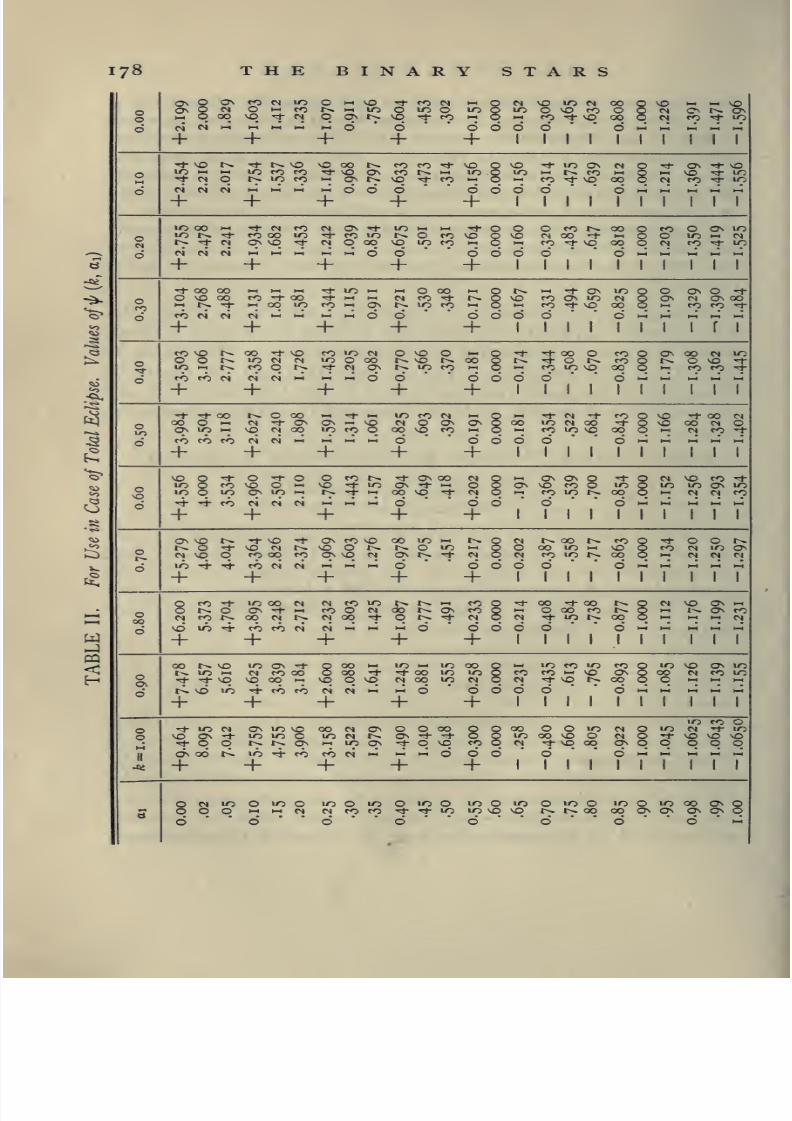
8/2/2019 The Binary Stars 1918
http://slidepdf.com/reader/full/the-binary-stars-1918 206/349
178 THE BINARY STARS
o o ON fe «s »o o ^ NO Tf re fs ^ ^ <N NO to N 00 ^ NO I-I vO
^Ov
gr< 9 ^ ^ t^ HH m o lO o m Q m O NO re o o r< OS r^ ON00 so rJ- <N o ON t>- so "^ re l-t o >-l re >* NO 00 o w re Tf to
o
+ +"
"
+
o o
+
o
+
o o1
o
1 1 1
o1 T r T T T
"t 'O l^ ^ l^ SO so 00 t^ re re rf so ^ sn <:* lO On (N ^ Tt OS ^^1o lO i-i »o ce re rh so On re r^ lO Q lO HH t^ re o NO lO
Tl- CS o l^ lO re ON 1^ so rf re o re -^ so 00 i r« re to
o+
N + "
+o o o
+o
+o o
1
o1 1 1
o
1 T T T T T
lO 00 ^ rf M re <N OS r^ »o ^ f* Tf „ o O re t^ 00 „ re o On to
%lo r^ Tf re 00 »o rf re ITi t^ o re so
Bso (N 00 rj- f*^ o to n
t^ "-t CS| ON so -^ M o 00 so lO re re Tj- so 00 ^ c< re "^ to
6 c< +"
"^
-f
o o o
+o o
1
o
1 1 1
o1 T T T T T
«+ 00 OO H >-l -! "+ \r> „ ^ o 00 1-1 o r^ •1 -^ OS lO ^ o ON o r1-
o O vO 00 re 'I- 00 «+ l_l <N re rf r^ NO re OS lO fS
gON <N ON 00 1
•-. t^ -^ -1 00 lO re t-l ON t^ lO re o re Tt so 00 re re ^6
+M M I-I I-I
+1-1
+" o o o
+o o
1
o
1 1 1
o1 T T T T T
^^ r^ 00 '^- so re »o <N o so o „ „ Tf Th 00 O re o On on <N» to
o t>. ID M r< lO o 00 r^ so r^ 00g
t^ ^ O t^ re »^ o NO "^ID H* t^ re O t^ Tf (S ON !>. m re n re »o so 00 o re re rt-
d (s» M C) i-i
+ -f
" o o4-
o o o1
o
1 1 1
o1 T T T T T
't '^ 00 I^ O 00 ^ ^ ^_ lO re <N „ ^ ^ Tl- (N) rh re ^ so -& 00 M
O 00 o hH n Tf ON ON so n o ON ON Q 00 lO <S 00 Tt 8 NO 00 rs»
oOS lO HH so (N 00 lO re o 00 so re o re «o so 00 <N re ^d
+fC r< (N 11
+ +o
+o
+o o
1
o1 1 1
o1 T r T T r
vO O Tt- O ^ O o re r^ rt- ON 00 M Q _ ON ON Oso re o
rh ^ (N so re rf
«^
lO Q rO so O i-i so Tf «o ON ^ )_l o Q On tog
to to On tolo 5 lO ON lO HH t^ rf 00 so ^ n 6 re »o t^ 00 (S M re
6 ^ "* re fS C< P< M M hH o o o o o HH t_l l_l hH H4
+ + + + + 1 1 1 1 1 1 1 1 1 1
J^^r^ 'd- so + ON re so OO lO ^ t^ „ <N r^ 00 t^ re ^ Ti- o o r^-+ SO fN t^ so o r>. r^ o lO
go 00 »o I-I so ^ re (N to ON
(S vO o re 00 re ON so M ON t^ "^- c< n re lo r^ 00 i rj C4 cs
6 ID r*- Tt re M <N l_ M 1^ o o o o o ol_l
^|_4 |_4 H^
+ + + + + 1 1 1 1 1 1 1 1 1 1
8 f:^
-t lO 00 fS <N re iOc5^
r^ ^ re ^ Tt- 00 Tt- 00 1-- f, (N NO ON ^o OS <1- I-I re o <N r>. as re
8O 00 re t^ Q ON re
<s rn t^ 00 <N 1^ M 00 '+ o t^ -t <s M Ti- lo r^ 00 o t-l •-I CSI
6 vO »0 Tf- re re <N M l_l HH HH o o o o o o )-l HH I-I I-I HH
+ + + + + 1 1 1 1 1 1 1 1 1 1
00 r>. so lO On -^
g00 J_ lO ^ lO 00 „ ^ lO re lO re ^ to NO ON to
t^ lO l_t <N re OO 00 Tt- Tf 00 U-5 lO o re re 11 NO On o 00 <N re to
0\Tf Tl- O so 00 •-• so o NO C) 00 ID c< o r< Tt- so t^ 00 (J o
6 t>. SO lO rf re re rs n l_l l_l o o o o o o HH l_l HH tH H4
4-
+ +4-
+1 1 1 1 1 1 1 1 1 1
to re oTj- \n M ON lO so 00 rj OS o o 00
8o 00 o o »o M o to (N "I- to
-^J"I- lO lO o m n r^ ON ^ -+
8lO 00 so O M
o^ so NO sO
o t^ t^ ON lO ON ^ o NO re (S ^ NO 00 OS o o o o
II
ON 00 t^ ID n- re re (N H4 )_l o o o o o HH hH i-l l_l HI
+ + + + + 1 1 1 1 1 1 1 1 1 1
o n lO O lO o ir> o lO o lO o lO o lO o to o to o to 00 OS8
cto o o l-< hH d M re re ^ rl- lO lO so so i-* r^ 00 00 OS ON ON ON
o o o o o o o o l-H

8/2/2019 The Binary Stars 1918
http://slidepdf.com/reader/full/the-binary-stars-1918 207/349
THE BINARY STARS
TABLE IIo
For Computing the Elements in the Case of Total Eclipse
179
k Mk) <t>t{k)
1.00 0.380 0.939
0.95 .401 .894
.90 .417 .848
0.85 0.427 0.802
.80 431 .755
•75 431 .709
0.70 0.427 0.663
.65 .419 .617
.60 .406 .572
0.55 0.390 0.527
.50 .371 .482
45 .349 436
0.40 0.323 0.390
.35 .294 .345
•30 .262 .298
0.25 0.226 0.250
.20 .187 .202
•15 .145 .153
O.IO O.IOO 0.103
.05 .052 .052
.00 .000 .000

8/2/2019 The Binary Stars 1918
http://slidepdf.com/reader/full/the-binary-stars-1918 208/349
i8o THE BINARY STARS
TABLE A
Loss of Light Corresponding to an Increase Am in Stellar Magnitude
Am I 2 3 4 5 6 7 8 9
0.0 o.oooo 0.0092 0.0183 0.0273 0.0362 0.0450 0.0538 0.0624 0.0710 0.0795
.1 .0880 .0964 .1046 .1128 .1210 .1290 .1370 .1449 .1528 .1605
.2 .1682 .1759 .1834 .1909 .1983 .2057 .2130 .2202 .2273 .2344
•3 .2414 .2484 .2553 .2621 .2689 .2756 .2822 .2888 .2953 .3018
4 .3082 .3145 .3208 .3270 .3332 .3393 .3454 .3514 .3573 .3632
•5 0.3690 0.3748 0.3806 0.3862 0.3919 0.3974 0.4030 0.4084 0.4139 0.4192
.6 .4246 .4298 .4351 .4402 .4454 .4505 .4555 .4605 .4654 .4703
•7 •4752 .4848 .4848 .4895 .4942 .4988 .5034 .5080 .5125 .5169
.8 .5214 .5258 .5301 •5344 .5387 .5429 .5471 .5513 .5554 .5594
•9 .5635 .5675 .5715 .5754 .5793 .5831 .5870 .5907 .5945 5982
I.O 0.6019 0.6055 0.6092 0.6127 0.6163 0.6198 0.6233 0.6267 0.6302 0.6336
I.I .6369 .6403 6435 .6468 .6501 .6533 .6564 .6596 .6627 .6658
1.2 .6689 .6719 .6749 .6779 .6808 .6838 .6867 .6895 .6924 .6952
1.3 .6980 .7008 •7035 .7062 .7089 .7116 .7142 .7169 .7195 .7220
1.4 .7246 .7271 .7296 .7321 .7345 .7370 .7394 .7418 .7441 •7465
1-5 0.7488 0.751 0.7534 0.7557 0.7579 0.7601 0.7623 0.7645 0.7667 0.7688
1.6 .7709 .7730 .7751 .7772 .7792 .7812 .7832 .7852 .7872 .7891
1-7 .7911 .7930 .7949 .7968 .7986 .8005 .8023 .8041 .8059 .8077
1.8 .8095 .8112 .8129 .8146 .8163 .8180 .8197 .8214 .8230 .8246
1.9 .8262 .8278 .8294 .8310 .8325 .8340 .8356 .8371 .8386 .8400
2.0 0.8415 0.8430 0.8444 0.8458 0.8472 0.8486 0.8500 0.8514 0.8528 0.8541
2.1 .8555 .8568 .8581 .8594 .8607 .8620 .8632 .8645 .8657 .8670
2.2 .8682 .8694 .8706 .8718 .8729 .8741 .8753 .8764 .8775 .8787
2.3 .8798 .8809 .8820 .8831 .8841 .8852 .8862 .8873 .8883 .8893
2.4 .8904 .8914 .8924 .8933 .8943 .8953 .8962 .8972 .8981 .8991
2.5 0.9000 0.9009 0.9018 0.9027 0.9036 0.9045 0.9054 0.9062 0.9071 0.9080
Forvalues of
Amgreater
than 2.5,the loss of light is
0.9000plus
j^of
the loss of light corresponding to Am — 2.5.

8/2/2019 The Binary Stars 1918
http://slidepdf.com/reader/full/the-binary-stars-1918 209/349
THE BINARY STARS
TABLE B
Values of d — Sin 6
i8i
0.0 0.1 0.2 0.3 0.4 0.5 0.6 0.7 0.8 0.9
0.00 0.0000 0.0002 0.0013 0.0045 0.0105 0.0206 0.0354 0.0558 0.0826 0.1 167
.01 .0000 .0002 .0015 .0049 .0114 .0218 .0372 .0582 .0857 .1205
.02 .0000 .0003 .0018 .0055 .0122 .0231 .0390 .0607 .0888 .1243
.03 .0000 .0004 .0020 .0060 .0131.0244 .0409
.0632 .0920 .1283
.04 .0000 .0005 .0023 .0066 .0141 .0258 .0428 .0658 .0953 .1324
0.05 0.0000 0.0006 0.0026 0.0071 0.0151 0.0273 0.0448 0.0684 0.0987 0.1365
.06 .0000 .0007 .0029 .0078 .0161 .0288 .0469 .0711 .1022 .1407
.07 .0001 .0008 .0033 .0084 .0171 .0304 .0490 .0739 .1057 .1450
.08 .0001 .0010 .0037 .0091 .0183 .0320 .0512 .0767 .1093 .1494
.09 .0001 .0011 .0041 .0098 .0194 .0337 .0535 .0796 .1130 .1539
To illustrate Russell's method I have chosen his orbit of
W Delphini, which is a "typical Algol variable with a deep
primary minimum, showing a constant phase, and little or no
9'?o
1090
u^o
jaiPo
--X V, ^,--
\ /
\^^ n a
-o?3 -o?2 -o4j o?o +o?i +o*a o'?9
Figure ii. Light-Curve of the Principal Minimum of W Delphini

8/2/2019 The Binary Stars 1918
http://slidepdf.com/reader/full/the-binary-stars-1918 210/349
1 82 THE BINARY STARS
secondary minimum." Its light curve, "defined by the 500
observations by Professor Wendell, with a polarizing photo-
meter, which are published in the Harvard Annals, 69, Part i,"
TABLE a
Observed Magnitudes
Phase Mag.No.
Obs.0.--C. Phase Mag.
No.
Obs.O.-C.
-0^2894 9.41 6 + "01 + 0^0560 11.76 7 ^-o^^oi
.2637 9.49 5 + .02 .0659 11.58 8 + .01
.2458 9.58 5 + .04 .0753 11-33 7- .04
.2306 9.59 4- .01 .0859 II. 14 5 — .02
.2200 9.67 5 .00 .0937 10.97 5 - .05
.2106 9.73 8 + .01 .1036 10.88 8 + .02
.2007 9.79 10 .00 .1147 10.73 8 + .05
.1911 9.88 12 + .02 .1246 10.56 12 + .03
.1817 9-95 10 + .01 .1351 10.39 14 .00
.1718 10.02 8 .00 .1445 10.31 II
-f.04
.1615 10.16 17 + .04 .1546 10.13 10 — .02
.1506 10.23 14 .00 .1641 10.10 II + .04
.1396 10.37 14 + .01 .1744 9.97 10 .00
.1311 10.44 16 —.03 .1847 9.90 9 + .02
.1212 10.59 17—
.03 .1941 9-79 9 — .02
.1121 10.78 14 + .01 .2050 9.71 8 — .02
.1013 10.91 17—
.04 .2157 9.71 6 + .04
.0906 II. 12 14- .01 .2242 9.63 8 + .01
.0809 11.30 10 — .02 .2345 9.57 7 .00
.0715 11.51 12 .00 .2507 950 7 .00
.0617 11.69 10 .00 .2708 9.48 7 + .03
.0509 11.88 7 .00 .2811 9.43 4 + .02
.0313 12.05 5—
.04 .94 9.42 5 4- .02
.0169 12.08 4— .02 1.90 9-35 5 - .05
— .0082 12.07 7—
.03 2.04 9.41 7 + .01
+ .0060 12.16 5 + .06 2.67 9.38 5— .02
.0139 12.09 4— .01 3.04 9.42 3 + .02
.0261 12.03 5 - .07 4.04 9-44 6 + .04
.0356 12.02 6 —.03 4.48 936 7
- .04
+ .0460 11.87 6 -.04
is shown in Figure 1 1 . The observations have been combined
into the normal places given in Table a, on the basis of a
period of 4.8061 days, which was found to require no correction.

8/2/2019 The Binary Stars 1918
http://slidepdf.com/reader/full/the-binary-stars-1918 211/349
THE BINARY STARS 183
From the thirty-eight observations outside minimum we find the
magnitude during constant light to be 9^395 =t 0.009. There is no
evidence of any change during this period. With a circular orbit, the
secondary minimum should occur at phase 2^40. As none of the ob-
servations fall within 0^27 of this, they give us no information whether
such a minimum exists. The light-curve of the principal minimum is
very well determined. The eclipse lasts from about — 0^28 to + 0^28,
and there is a short constant period at the middle, of apparently a little
less than one-tenth the total duration of the eclipse. The mean of the
twenty observations lying within 0^02 of the middle of eclipse gives
for the magnitude at this phase 12^10 ±0.014. The range of variation
is therefore 2']'70, and the light-intensity at minimum 0.0832 times
that at maximum. This shows at once that the eclipse is total, for if
it was annular, the companion (even if perfectly dark) must cut off at
least 0.917 of the light of the primary, and hence its radius cannot be
less than 0.956 times that of the latter. In such a system the duration
0.044of the annular phase could not exceed ,
or 0.022 of the whole1.956
duration of eclipse. The observed constant phase is almost five times
as long as this.
The brighter star therefore gives 0.9168 of the whole light of the
system, and if isolated would appear of magnitude 9.49; while the
fainter but larger star which eclipses it gives out only one-eleventh as
much light, and when seen alone at minimum is of magnitude 12.10.
The loss of light (i — 1) at any given time, /, will be o.9i68ai,
since ai is the percentage of obscuration. For a series of values
of ai we tabulate the values of (i— 1) and then take from
Table A the corresponding changes of magnitude and apply
them to magnitude 9.4. Next, from the free-hand curve
drawn to represent the data of observation, we read ofT the
epochs ti and /2 at which the magnitudes so computed are
reached before and after the middle of eclipse. Half the
difTerence of /i and ^2 may be taken as the interval / from the
middle of eclipse to each phase and the corresponding value of
d formed from
2 TT
6 = / = 1.3065^, where d is expressed in radians and t in days.
With the aid of Table B sin 6 is found and then sin^ 6. These
quantities are all entered in Table b.

8/2/2019 The Binary Stars 1918
http://slidepdf.com/reader/full/the-binary-stars-1918 212/349
1 84 THE BINARY STARS
.• Tf lO O M ••
VO O O 00 'O vOlO lO lO Tt- tJ- to
6
•• »0 00 ••
00 N M OlO lO lO »o
00 O (N •-<
00 Th O ON O ^(S vO On N 00 rc
+o o
+
NO "^ Ot^ ON QrO NO Odo-:I I I
lO t^ 00 -^lO t^ w o•-« N CO Th
I I I I
lO ^ l-H to t^ ro C> r^ On O (N
O 00 ON ro O ON <> ON t>. lO On <N| rj- NO
= «
Tj- ro fN«
^ 5^
•-1 r« ci ro fO CO
oo
o qd
O O O O q q
I I I I I I I
rl- O O (N NO f^ ON r< o ^^ HH O O^ t^t^ »0 NO O 1^ NO NO r^ On 1-1 t>> •^ n o
? ^ q S-iP ^ S?o o o q q q 8 8 8. 8
.•Ttoo•-«NO^Ol-«»-'•-lT^NOC^NO•^OnOOO CS t>.fONO00 lOfOrOfONO
ONtOONNOrJ-tHONNO
~ ~
rOfOC<NP*N>-<M6 *
fO O 00 vO lO C<"-I •-> o o o o
.. lOOO O O -^O Tt-00008N- iOfO<Orhr^l^Tj-oo
lori ooono t1-(n orO M <N n 1-1 f
n O t^ NO tJ- ro "-I
-I 1-1 o o o o o
• • o mioThCNjNO o o Ti-ioloo ••
"^Thoo 1-^000000 t^r^M too fO>-iO lO(N).OOONO Tj-(NJ OoonO lOThMrONM<N'-'»-i'-i'-i'-iOOOOOo
I1
8 100 OvvOnOnO ThiDM ThTt-«00O <Nj tJ-OnnOnO >- rOONM OOOO O
TfiONO t^OO O CNJ »O00 MnOOO On*-"
S'dNONONONd666i-:>-J«>-:r<On i-ii-ii-thHi-ii-ii-ii-iMi
r^-^o t^rho t>.Tj-o1-1 rOiOvOOO O M r0»0OnoO t^NO lOiOrJ-rorj t^ON©O "-i M fO-^iONO 1^000000 O^ O-^
ON lO vO 00O 00 t^ NO
O «d
»0 NO 1^ 00
be
.S"^
i ^
-I60 ao rt
.t: a
a o<v a05 B
1^E rt
3 :5
« 6
8/2/2019 The Binary Stars 1918
http://slidepdf.com/reader/full/the-binary-stars-1918 213/349
THE BINARY STARS 1 85
From the values of ti and <2 it appears that the observed curve is
remarkably symmetrical, and that the actual epoch of mid-eclipse is
0.0015 days earlier than that assumed by Wendell. The times of
beginning and ending of the eclipse cannot be read accurately from
the curve and are marked with colons to denote uncertainty.
From the values of sin^ 6 we have now to find k with the
aid of Table II. From equation (13) we have
sin' 9i — A^(*.ai)=
B
hence, if we let A be the value of sin^ 6 when ai = 0.6 and A — Bits value when ^2 = 0.9, we may find a value of k for every
tabulated value of ai by inverse interpolation in Table II.
Thus, taking A = 0.0369 and B ( = sin^ 62 — sin^ ^3) = 0.0258,
as given by our curve, we find for ai = 0.0 that\f/
{k, ai) =
+ 4.28:, and hence, from the first line of Table //, k = 0.56:.
Colons are here used because the values of k are less accurate
when the tabular differences of\f/
{k, ai) are small.
The values of k are seen to be fairly accordant except for
those corresponding to values ai near 0.6. Inspection of
Table II "shows that this discrepancy may be almost removed
by increasing all the values of xj/ by 0.024 — which may be
done by diminishing A by 0.024^. Our new value of A is
therefore 0.0363." The new set of ^'s are found to be dis-
cordant for values of ai near 0.9; "but by diminishing B by
2}^ per cent, [giving B = 0.0252], and hence increasing all
the computed values of xf/ in the corresponding ratio, we obtain
a third approximation of a very satisfactory character." The
general mean is now k = 0.528.
With these final constants, A = 0.0363, B = 0.0252, k =
0.528, we may compute a theoretical light-curve andalso the
elements of the system from equation (14). Table c gives the
second and third approximations to the value of k and the
data for the final light-curve.
Plotting the magnitudes computed in Table a against the epochs
— 0*10015 ±/, we obtain the computed light-curve. The residuals
(O. — C.) are given in the last column of Table a. Their average value,
regardless of sign, is 0^020.
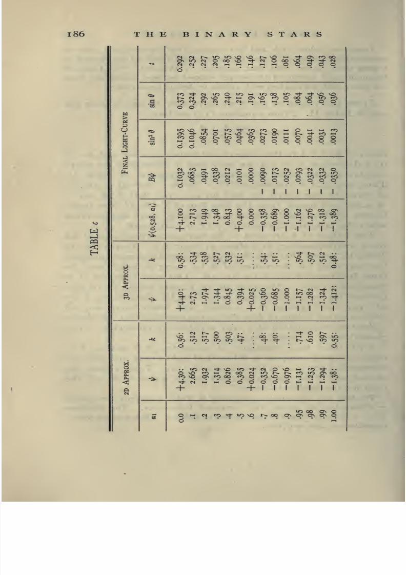
8/2/2019 The Binary Stars 1918
http://slidepdf.com/reader/full/the-binary-stars-1918 214/349
1 86 THE BINARY STARS
r< M t^ »0 lO VO VO t^ VO •* Ov to 00On lO (N O 00 VO rt- « 2
oo vO Tt- rh Mq q q q(S (M rj M M i-< q
6
^ ro "«*• M ID O lO HH lO 00 xn Th rh VO VOr>. (s On VO Tf M Ov VO to o 00 VO >o to
c CO fO M M n CI hH l-H q q q qw d d
.
a
%
u ^ IC vO tJ- i-i lO Th to to o hH O t-i 1-1 toON * ir> o t^ VO VO t^ Ov HH t^ -^ to i-i
.Sto o
^ s-??q
qq q
q q S
q'»
o oJh)
<z
feCS ro t-i oo H >-i Q O to r« to (v» (S O
^ to 00 Ov to "-I Og
Ov t^ lO Ov n to lo
2 ^rt- to n HH o ^ n M to to to
tt) q q q q o q q q q q o od
1 1 1 till^_^
ti O rO ^^^8 Q 00 Ov Q (M VO 00 Ov. O -, Q lO 00
8
VO 1^ HH 00
00 1-1 r^ Ov to 00 rt- o to VO HH n to tolO 4 ci H^ M d d d d d t_^ M 1-4 M 1^
3 + + 1 1 1 1 1 1 1
^
•• "^ 00 1^ M •• Th 1^ M ..
00 to to M to "-I Tf hH VO O HH 00Jii lO lO ID lO »0 ID lO lO lO lO lO -^
X d.
dos?CLi
<Tf rh ir> rt- lO O lO Q 1^ M rh
<v)
Q d rO l^ -rh 'i- Ov (V| \0 00§
lO 00 M i-i
ro -^ Tj- I^ Ov to 00 to o to VO•I
n to T*-
-4- cl >^ .:, 6 6 d d d HH HH hH •-( 1-^
+ + 1 1 1 1 1 1 1
.. C)H^ O O 1^
rf- O »^ ..
\D >-, 00 O M HH ON in-Oi
dlO lO lO '^ 't ^ t^ VO »0 lO
'' d
><
OaOh
Ok
.. lO W Tf- VO «0 <t n o VO •-I ro tJ- ..
O VO to •- (N 00 (N to r^ l^ tO lO Ov 00
-^ fO VO Ov to 00 to o to VO Ov *>^ CJ cj to
< 4 pi h; M d d d d d d i4 )-? K-i i-i
+ + 1 1 1 MilN
to 00 ov OOv qv Ov qO w W to ri- lO vq ^ 00 as
d

8/2/2019 The Binary Stars 1918
http://slidepdf.com/reader/full/the-binary-stars-1918 215/349
THE BINARY STARS 187
From Table I la we find for k = 0.528, tt>\{k) = 0.382, 4>2{k) =
0.507; whence
B^ot^* = ~7i;
- ^ = 0-0133. cot t = O.I 15, t = 83° 25'.
Br^ cosec^ i = —— = 0.0660, r^ = 0.0652, ri = 0.256,
and finally
r% = ^ri = 0.135.
In other words, we have, taking the radius of the orbit as unity,
Radius of larger star 0.256
Radius of smaller star *
'
0.135
Inclination of orbit plane 83"25'
Least apparent distance of centers 0.114
Light of larger star 0.0832
Light of smaller star 0.9168
[Period of revolution 4.8061 days]
At the middle of eclipse, the larger star overlaps the other by only
0.007 of the radius of the orbit, or about one-twentieth of the radius
of the smaller body, so that the eclipse is very nearly grazing. The
smaller star gives off eleven times as much light as the other, and ex-
ceeds it forty-fold in surface-brightness.
The loss of light at secondary minimum should be k times the light
of the fainter star, or 0.023 of that of the system. The corresponding
change in stellar magnitude is 0.027, which could only be detected by
refined observations.
In an earlier paper Russell gives the equations which deter-
mine the density of the components relatively to the density
of the Sun in terms of the orbit elements.
Let the total mass of the system be m, that of the larger star my
and that of the smaller m{\ — y). If a is the semi-axis major of the
orbit, we shall have a = KwYi P^i, where X is a constant depending
on the units of measurement. If we choose the Sun's mass, the Sun's
radius, and the day as units, then for the Earth's orbital motion
a = 214.9, P = 365.24, whence K = 4.206.
In determining the elements of the system, we have taken a as our
unit of length. The actual radius of the larger star is therefore an,
and its volume in terms of that of the Sun is K^mP^ri^, or ^44 mp^ri\

8/2/2019 The Binary Stars 1918
http://slidepdf.com/reader/full/the-binary-stars-1918 216/349
l88 THE BINARY STARS
yIts density pi is therefore pi = 0.01344 > and similarly, of the
I — y.smaller star p2 = 0.01344 .
The actual densities can be computed only when the ratio
of masses of the two stars is known. Assuming the two com-
ponents of W Delphini to be of equal mass, the equations give
r-©
oSUN
:--©
Figure 12. The Sj^stem of W Delphini. The relative orbits of the bright star
are shown; the upper diagram representing the elements as given in the
accompanying solution, the lower, Shapley's elements on the assumption that
the stars are darkened to zero at the limb. The diameters of the disks of
stars and Sun are drawn on the same scale; the three bodies have the same
mass, but the stars are less dense than the Sun.—From Shapley's article in
Popular Astronomy, vol. 20, p. 572, 1912
O.I 18 of the Sun's density for the density of the smaller and
brighter star and 0.017 ^oi" the density of the larger and
fainter one.
Dr. Harlow Shapley, who was associated with Professor
Russell in the theoretical investigations which have been
described above, has applied the theory in a very comprehen-
sive manner, and has published (in No. 3 of the Contributions
from the Princeton University Observatory, 191 5) "A Study of
the Orbits of Eclipsing Binaries" containing orbits for ninety
different systems, with a thorough discussion of the results.
It is not expedient to copy his table of orbits here, for, aside
from the space required, it would be necessary to extend con-
siderably the discussion already given, in order to make all of

8/2/2019 The Binary Stars 1918
http://slidepdf.com/reader/full/the-binary-stars-1918 217/349
THE BINARY STARS 189
the details of the table readily intelligible. Some general
statements concerning the table and Shapley's discussion must
suffice.
Since there is both theoretical and observational support
for the hypothesis that the disks of eclipsing variable stars
are not uniformly illuminated but are darkened toward the
limb, like our Sun, by the increased absorption of their en-
veloping atmospheres, Shapley gives for each system at least
two orbits, one for the hypothesis of uniform illumination, the
other for the hypothesis of darkening toward the limb. Whenthe nature of the data does not permit a definitive solution,
several orbits are given to show the limits within which the
elements may be varied. In all, more than 200 orbits are
tabulated, nearly all of them computed by Shapley himself.
The results seem to justify the conclusion that darkening
toward the limb characterizes practically all of the stars under
discussion, but the degree of darkening cannot as yet be deter-
mined with any certainty.
Shapley finds a distinct correlation between the range of
light variation and the relative sizes of the two components;
when at principal minimum the star is two magnitudes or more
fainter than when at maximum, the brighter star is never the
larger, and it is only rarely the larger when this range is in
excess of one magnitude. On the other hand, when the rangeis less than 0.7 magnitudes, "there is not a single system
known where the fainter star is the larger."
There is a positive indication in all but a very few cases
"that the fainter star is self-luminous and in no case is it nec-
essary to assume one component completely black. In about
two-thirds of the systems the difference in brightness of the
components does not exceed twomagnitudes, and no observed
difference is greater than four magnitudes." A large percen-
tage of the visual binaries have a far greater difference of
brightness between the two components. The fainter star, in
the eclipsing systems, has always been found to be redder, and
hence probably of a later class of spectrum than the bright
star, whenever it has been possible to determine the relative
color-index of the two components.

8/2/2019 The Binary Stars 1918
http://slidepdf.com/reader/full/the-binary-stars-1918 218/349
190 THE BINARY STARS
The great majority of the ecHpsIng binaries at present
known belong to the spectral classes B and A. When the den-
sities are computed, on the assumption that the mass of each
component is equal to that of the Sun, it is found that the
densities of stars of spectral classes B and A lie mainly between
0.02 and 0.20 of the density of the Sun. The range in density
of the small number of eclipsing binaries of spectral classes
F, G, and K is much greater, exceeding the density of the Sun
in one system (W Ursae Majoris, Class G) and falling below
o.oooi of the Sun's density in two instances, while in only twodoes it fall within the limits 0.02 and 0.20.
Definite values for the eccentricity of the orbit could be
determined in only about a dozen systems, the maximum value
being 0.138 (for R Canis Majoris); a number of systems are
known to be practically circular, but in most systems the evi-
dence on this point is insufficient. However it may safely be
said that the departure from a circular orbit is never very great.
Whenever there was evidence of ellipticity of the disks of the
two components, caused by their mutual attraction, it was
found that "the degree of the elongation depended directly
upon the relative distance separating the two stars", and that
the numerical values were in good agreement with Darwin's
theoretical values for homogeneous incompressible fluids. The
ellipticity has rarely been measured when the distance between
the components equals or exceeds the sum of their radii.
Russell and Shapley have also studied the distribution of
the eclipsing binaries in space and reference to their results
will be made in a later chapter.
Stebbins, among others, has reminded us that every short
period spectroscopic binary star would be an eclipsing variable
to an observer in the plane of its orbit, and he has drawn the
corollary, that probably a number of eclipsing variables with
relatively small range in brightness exist among the known
spectroscopic binaries. Acting upon this conclusion, he took
up the examination of several such systems with the sensitive
selenium-cell photometer which he had developed, and was
able to show that the first two studied were in fact eclipsing
systems. It is not to be expected that this record will be

8/2/2019 The Binary Stars 1918
http://slidepdf.com/reader/full/the-binary-stars-1918 219/349
THE BINARY STARS I9I
duplicated; indeed, Stebbins himself found that many of the
systems examined later gave no evidence of light variation.
Nevertheless, the field is a promising one, but the instrumentsdemanded for its cultivation are the very sensitive modern
photometers. Excellent work, however, may be done with any
good photometer on the eclipsing binaries of greater light
range, and we may expect a considerable addition to the num-
ber of orbits of such systems in the near future if the observa-
tions are carried out systematically. The description of the
instruments and methodsof
observation may be foundin
books on variable stars like Miss Furness's "Introduction to
the Study of Variable Stars" or Father Hagen's "Die Verander-
liche Sterne."
REFERENCES
Russell, H. N. On the Determination of the Orbital Elements of
Eclipsing Variable Stars. Astrophysical Journal, vol.35, p. 315,
191 1 ; vol 36, p. 54, 1912.
Russell, H. N. and Shapley, H. On Darkening at the Limb in
Eclipsing Variables. Astrophysical Journal, vol. 36, p. 239 and
385. 1912.
Shapley, H. The Orbits of Eighty-seven Eclipsing Binaries—A Sum-
mary. Astrophysical Journal, vol. 38, p. 158, 1913.
.
A Study of Eclipsing Binaries. Contributions from the Prince-
ton University Observatory, no. 3, 1915.
These papers contain references to many others by the
same, and by other writers. Attention should also be called to
the recent Bulletins of the Laws Observatory, University of
Missouri, for Professor R. H. Baker has entered upon an
extensive program of work on eclipsing binaries and the results
are being published in those Bulletins.

8/2/2019 The Binary Stars 1918
http://slidepdf.com/reader/full/the-binary-stars-1918 220/349
CHAPTER VIII
THE KNOWN ORBITS OF VISUAL ANDSPECTROSCOPIC BINARY STARS
The orbits of 112 visual and of 137 spectroscopic binary
star systems have been computed by different astronomers,^
by means of the methods outHned in preceding chapters.Many of these orbits, especially those of spectroscopic binaries
and of short period visual systems, may be regarded as de-
finitive, others, especially those of the very long period
visual binaries, have little or no value. Every computation
was undertaken with the immediate object in view of repre-
senting the observed motion and of predicting the future
motion in the particular system on the assumption that the
controlling force is the force of gravitation; but back of this
lay the broader motive of providing additional data for the
study of the greater questions of stellar motions and, particu-
larly, of stellar evolution. In the present chapter I shall
present some relations and conclusions which may be deduced,
with more or less certainty, from the computed orbit elements,
but their interpretation and their bearing upon the problems
of the origin of the binary stars and their relations to single
star systems will be left for a later chapter.
Table I gives the elements of eighty-seven of the visual
binary star systems, divided into two groups, the first con-
taining the orbits which are at least fairly good approxima-
tions, the second, the less accurate orbits. The dividing line
is not a very definite one; several orbits included in either one
of the two groups might with perhaps equal propriety find a
place in the other. In each group the systems are arranged
in the order of right ascension, and the columns, in order, give
the star's name, the position for 1900.0, the magnitudes and
spectral class (taken from the Harvard Photometry as far as
1 Written in October, igi?- Tables I and II, containing the orbits of these stars, are
placed at the end of the book for convenient reference.

8/2/2019 The Binary Stars 1918
http://slidepdf.com/reader/full/the-binary-stars-1918 221/349
THE BINARY STARS I93
possible), the orbit elements, and the name of the computer.
Only one orbit is given for each system, the most recent one,
unless there is a special reason for choosing an earlier one.For many systems ten or more orbits have been published.
References to the earlier orbits may be found in Burnham's
General Catalogue or in Lewis's volume on the stars of the Men-
surae Micrometricae. The later orbits are, for the most part,
published in the Astronomische Nachrichten, the Astronomical
Journal, and Volume 12, of the Publications of the Lick Obser-
vatory. The orbits which have been computed for twenty-five
other systems are omitted because the data upon which they
are based are entirely inadequate, and any conclusions drawn
from the results would be entitled to no weight whatever.
Perhaps the best observed among the omitted systems is the
well known binary o- Coronae Borealis; using practically the
same observations, Lewis finds the revolution period to be 340
years, while Doberck's value is 1,679 years!
For reasons already given, the orbits of the spectrographic
binary stars are, in general, more accurate than those of the
visual binaries, and only five of the 137 are assigned to the
second group of Table IL Of these, a Persei is excluded from
the main table because there is still a reasonable doubt as to
whether or not it is a binary at alP; ^ Canis Majoris and
p Leonis because the orbits are avowedly only rough approxi-
mations, and the two long period systems, a Orionis and a
Scarpa, because Lunt's ' recent discussion shows that the data
on which the orbits rest are inadequate for good solutions. It
does not follow that all of the orbits retained in the main divi-
sion of the table are of equal value; doubtless, several should
properly be transferred to the second section for reasons similar
to those given for the transfer of a Orionis and a Scorpii. A
few others depend on the H and K lines of calcium only, lines
which exhibit anomalies not yet perfectly understood; and
one system, <^ Persei, has recently been pronounced as still "a
complete riddle." The results which follow, however, are not
afifected by their retention.
^Lick Observatory Bulletin, 7, 99, 1912.
» Astrophysical Journal, 44, 250, 1916.

8/2/2019 The Binary Stars 1918
http://slidepdf.com/reader/full/the-binary-stars-1918 222/349
194 THE BINARY STARS
As in the table for the visual systems, the stars are arranged
in order of right ascension. The columns give, consecutively,
the star's name, the position for 1900.0, the magnitude and
spectrum (from the Harvard Photometry) the orbit elements
and the computer. Here again but one orbit is given, though
two or more have been computed for several systems. In a
number of systems, however, the second spectrum is visible
on the plates, and values of the elements of the secondary,
which differ from those of the primary, if given by the com-
puter, are entered in the line below the principal orbit. In a
few instances, also, the elements of a third body in the system,
or of a secondary oscillation in the orbit are added.
RELATIONS BETWEEN PERIOD AND ECCENTRICITY
Certain striking characteristics of the orbits in the two
tables are recognized on the most casual inspection; for ex-
ample, the eccentricity of the visual orbits is generally large,
that of spectroscopic orbits generally small; the periods of
the former are long—the shortest known so far being 5.7 years
(5 Equulei)—those of the latter generally short, ranging from
about five hours to less than 150 days with but few exceptions.
See, Doberck, and many other recent writers have called
attention to the high average eccentricity of the visual binary
star orbits, See finding in this fact strong support for his earlier
theory (since abandoned by him, but not entirely by others)
of the origin of the binary star systems. The average value of
the eccentricity for the eight major planets in the solar system
is only 0.06, and the largest, for Mercury, is only 0.206;
whereas the average of the sixty-eight values in the first part
of Table I is 0.48, agreeing very precisely with the value See
found in 1896 from the orbits of forty systems. The average
value of e for the nineteen systems in the second group is evenhigher, exceeding 0.61.
On the other hand, the average eccentricity of the 132 orbits
of spectroscopic binaries included in the main division of
Table II is only 0.205, and of the five more uncertain orbits
only 0.30. Recalling the fact that the periods of the visual
binaries are, on the average, much greater than those of the

8/2/2019 The Binary Stars 1918
http://slidepdf.com/reader/full/the-binary-stars-1918 223/349
THE BINARY STARS 195
spectroscopic, it is natural to try to establish a relation between
the two elements. Doberck long ago presented evidence tending
to show that the eccentricity of the visual binaries increased
with the length of the period; Campbell, Schlesinger, Luden-
dorff and others have shown that a similar relationship exists
among the spectroscopic binaries.
Examining the data now available, we find that the relation-
ship is established beyond question. Omitting the twelve
Cepheid variable stars ^ and RR Lyrae, a 'cluster type' vari-
able, because the peculiarities in these systems seem to differ-
entiate them too much from the other spectroscopic binaries
to justify their inclusion in studies of the relations between
orbit elements, I have classified the remaining 119 stars in the
main part of Table II according to period and eccentricity and
give the results in Table III. Table IV contains a similar
grouping for the sixty-eight visual binaries of the first part of
Table I.
TABLE III
Periods and Eccentricities in Spectroscopic Binaries
d
0-5
d
S-io
d
10-20
d
20-50
d
50-150
d
150+Sums
o-.io 40 9 6 3 3 I 62
.10-. 20 5 4 I 2 4 16
.20-
.30 I 5 I I 2 2 12
.30-. 40 2 I 2 I 6
.40-. 50 I 2 I 3 7
.50-. 60 I 3 3 2 9
.60-. 70 I I 2
.70-. 80 3 I 4
.80-. 90 I I
.90-1.00
Sums 46 19 12 13 15 14 119
* /3 Cephei should perhaps be classified with the Cepheid variables, for according to
Guthnick, the light curve resembles that of variables of this class. The variation, however,
is only 0.05 magnitude, and in its spectral class and the characteristics of its orbit it differs
decidedly from the twelve Cepheids which I am discussing separately.

8/2/2019 The Binary Stars 1918
http://slidepdf.com/reader/full/the-binary-stars-1918 224/349
196 THE BINARY STARS
TABLE IV
Periods and Eccentricities in Visual Binaries
X y
0-50
y
50-100
y
100-150
y
150+Sums
O-.IO
.IC>-.20 5 I I 7
20-. 30 4 4
30-. 40 7 4 2 I 14
40-50 5 6 I 2 14
50-. 60 4 4 I 5 14
60-. 70 I I I I 4
70-. 80 3 3 I 7
80-. 90 I I I 3
90-1.00 I I
Sums 30 20 6 12 68
A more succinct summary may be made as follows:
TABLE V
spectroscopic Binaries
Number Average Period Average Eccentricity
d
46 2.75 0.047
19 7.80 0.147
12 1517 0.202
13 30.24 0.437
15 106.4 0.371
14 1.035- 0.328
Visual Binaries
30
20
6
12
0.423
0.514
0.558
0.529

8/2/2019 The Binary Stars 1918
http://slidepdf.com/reader/full/the-binary-stars-1918 225/349
THE BINARY STARS 197
To smooth the relationship curve let us combine lines 3 and
4, 5 and 6, and 9 and 10 of Table V; we then have:
TABLE VI
P e
Sp. Bin. 46 2.75 da. 0.047
19 7.80 0.147
25 23.00 0.324
29 555( = i-5y.) 0.350
Vis. Bin. 30 3i.3yr. 0.423
20 74-4 0.514
18 170 0.539
It is of interest, however, to note in Table V the definite maxi-
mum of e in spectroscopic binary stars with periods of from
twenty to fifty days, and the similar, but less marked, maxi-
mum in visual binaries with periods between 100 and 150 years.
The latter may be apparent, only, since but six stars are
involved. The rapid increase of e with lengthening P in the
first three lines of Table VI and the relatively slow increase in
the later lines is worthy of note.
The evidence from the less certain orbits may be added, for
the sake of completeness ; the three short period spectroscopic
binary stars have an average period of 5.5 days and an average
e of 0.36; while for the two long period ones the data are
p = 5.99 yr., 6 = 0.22. Had these results been included in
Table V the general order of the averages would not have been
affected. This remark holds also for the nineteen uncertain
orbits of visual binaries, but here the last two numerical values
would have been changed materially, for we have
6 stars average P 6'j .'j yr.
6 stars average P 118 yr.
7 stars average P 213 yr.
average e 0.51
average e o . 68
average e o. 65
The relationship so definitely established between the length
of the revolution period and the degree of ellipticity of the
orbit must have a physical significance.

8/2/2019 The Binary Stars 1918
http://slidepdf.com/reader/full/the-binary-stars-1918 226/349
198 THE BINARY STARS
RELATIONS BETWEEN PERIOD AND SPECTRAL CLASS
Dr. Campbell, In his study of the spectroscopic binary stars
found evidence of a relationship between the period and the
spectral class; taking the spectra in the order B, A, F, G, K,
and M the period increases as we pass from B toward M.
Before analyzing the present data to see whether they support
this conclusion, it should be said that In combining the various
Sub-classes, I have followed the Harvard Observatory system,
making Class B include Sub-classes O to B8, Class A, Sub-
classes B9 to A3, Class F, Sub-classes A5 to F2, Class G, Sub-
classes F5 to Go, Class K, Sub-classes G5 to K2, and Class M,
Sub-classes K5 to Mb. This differs somewhat from the group-
ing adopted by Campbell; a fact which must be kept in mind
if comparisons are made between his tables and those which
follow.^ It must also be noted that Table I contains a few
exceptional stars that cannot at present be fairly considered
in this connection. These are x Aurigae, Class Bi, whose
period of 655 days equals more than half the sum of all the
remaining forty-seven Class B periods; 7 Geminorum, Class
A, period 2,175 days, and e Ursae Majoris, Class A, period 4.15
years (= 1,515 days), respectively four and three times the
sum of the periods of the remaining thirty-six Class A stars;
and € Hydrae, Sub-class F8, with a period of 5,588 days, as
compared with 3,476 days for the sum of the remaining thirteen
Class G stars.
Omitting these four stars from Table II (e Hydrae is counted
with the visual binaries) and, as before, the Cepheid and
cluster-type variables, and counting the one Class M star with
Class K, we have the following results
« Campbell also includes a number of systems whose periods are known either definitely
or as 'short' or 'long', but for which no orbits have been computed.

8/2/2019 The Binary Stars 1918
http://slidepdf.com/reader/full/the-binary-stars-1918 227/349
THE BINARY STARS
TABLE VII
Spectroscopic Binaries
199
No. Class Av. P ' Av. e
48 B 26.76 da. 0.189
36 A 13-35 0.187
10 F 32.76 . 252
13 G 267.4 0.129
8 K-M 152.9 0.196
Visual Binaries
13 A 98.9 yr. 0.529
9 F 100.6 0.512
30 G 78.7 0.478
12 K 86.0 0.432
4 M 126.7 0.402
Table VII has several features of interest. In the first place,
it appears that if we divide the spectroscopic binaries into two
groups by a line between Classes F and G, those of the second
group have average periods decidedly longer than the periods
of those in the first ; but that in neither group does the period
increase, on the average, with advancing spectral class. In
the second place, we note that the distribution with respect
to spectral class is very different in the two setsof binaries,
the spectroscopic and the visual; spectra of early type pre-
dominate among the former, whereas there is not a single Class
B star among the latter, and nearly half the number belong to
Class G.
Looking over the list of spectroscopic binaries for which no
orbits have as yet been computed, I find that in fifty-three
cases either the approximate period or the note 'long' or
'short' is given. Classifying these according to spectrum, I find
B A F G K M
Period short 13 9 6 5
Period long I I 8 7 I
Several years ago I also tabulated the spectral classes of 164
visual binaries which show rapid orbital motion and found

8/2/2019 The Binary Stars 1918
http://slidepdf.com/reader/full/the-binary-stars-1918 228/349
200 THE BINARY STARS
that four were of Class B, 131 of Classes A to F (including
Sub-classes F5 and F8), 28 of Classes G to K (including K5)
and only one of Class M.In connection with the facts just stated it must be kept in
mind that spectroscopic systems of short period are more
readily discovered than those of long period, for not only is
the amplitude of the velocity curve greater, in general, in the
former but the variation in the velocity becomes apparent in
a much shorter time. We may expect relatively more long
period systems in future discoveries among stars of all classes
of spectra and hence an increase in the average values of the
periods. It should also be noted that the spectra of stars of
the later types, in general, show more lines, and these more
sharply defined, than the spectra of the early type stars. The
probable error of measure is therefore less and hence a variable
radial velocity of small amplitude may be unmistakable in,
say a Class G or K star, whereas one of equal amplitude may
escape recognition in a star of Class B. This might account
in part, for the relative numbers of the systems of long period
among the different classes of spectroscopic binaries, but it
obviously does not explain the very large relative number of
short period binaries of Class B. As for the visual binaries,
if we accept the current doctrine that the stars of Class B
and the brighter stars of Class M are the most remote we might
expect that some systems of these classes with periods of the
order of those given in the table would fall below the resolving
power of our telescopes. Allowing for the effects of these
factors, we may still conclude that, taking both the average
periods and the number of systems into account and also
the difference in these respects between the visual and
spectroscopic systems the evidence is definitely in favor of
an increase of the period of binary stars with advancing
spectral class.
In passing, attention may be called to the curious distribu-
tion of the eccentricities in Table VII ; the definite progression,
or rather retrogression, with advancing spectral class shown
by the visual systems is in marked contrast with the distribu-

8/2/2019 The Binary Stars 1918
http://slidepdf.com/reader/full/the-binary-stars-1918 229/349
THE BINARY STARS 201
tion among the spectroscopic systems. It is doubtful whether
any significance attaches to either.
THE DISTRIBUTION OF THE LONGITUDES OF PERIASTRON
In 1908 Mr. J. Millar Barr * called attention to a singular
distribution of the values of w, the longitude of periastron, in
those spectroscopic binaries whose orbits are elliptic. In the
thirty orbits available to him in which e was greater than 0.0,
twenty-six had values of co falling between 0° and 180° and
only four between180°
and 360°. Since there is no conceivablerelation between the position of the longitudes of periastron
in these orbits and the position of the Sun in space (except in
the case of the Cepheid variables), such a distribution is in-
herently improbable unless it is produced by some error of
observation. This, in fact, was Barr's conclusion—
"the elliptic
elements, e and w, as computed and published for the orbits
under notice, are probably illusory, the 'observed radial ve-
locities' upon which they are based being vitiated by some
neglected source of systematic error."
If this conclusion were well founded, it would be a serious
matter indeed, but both Ludendorff and Schlesinger have
shown that the one-sided distribution of periastra noted by
Barr "was nothing more than a somewhat extraordinary co-
incidence," for it becomes less marked as additional orbits are
considered. The data in Table II tend to confirm this state-
ment, though the inequality of distribution is not yet entirely
eliminated. Omitting the Cepheid variables and three stars
for which co might be taken on either side of the dividing line
(2 Lacertae, co = 180°, /3 Lyrae, w = 0°, and w Cassiopeiae, a
system with practically equal components either of which
might be regarded as the primary) we have 100 systems in
which e exceeds zero. Dividing these into two groups accord-
ing to the value of e, the values of a? are distributed in the four
quadrants as follows
1st 2nd 3rd 4th
c < 0.50 26 21 19 16
c^o.50 9 3 3 3
* Journal R. A. S. C, 2, 70, 1908.
8/2/2019 The Binary Stars 1918
http://slidepdf.com/reader/full/the-binary-stars-1918 230/349
202 THE BINARY STARS
The ratio of the number of oj's less than 1 80° to that of the co's
greater than this value is thus 47 : 35 and 12 : 6 in the two
groupsrespectively.
Doubtless, whenthe
number of knownorbits is doubled, these will both be reduced approximately to
equalities.
THE MASSES OF THE BINARY STARS
A knowledge of the masses of the stars is one of the funda-
mental requirements for a solution of the mechanical problems
of our stellar system, and this knowledge can be derived only
from binary stars. For this reason the methods by which wedetermine the absolute and the relative masses in both visual
and spectroscopic binaries, and the results which have been
obtained by their application, will be presented in some detail.
Unfortunately, the orbit elements alone do not afford all
the data necessary for the determination of either mass or
density. The well-known harmonic law D^ :d^= P^{M -\- Mi) :
p'^
{m -f mi), will give the mass of any system in terms of theSun's mass when the linear dimensions of the system as well as
the orbit elements are known. But. the semi-axis major of the
visual binary stars is known only in terms of seconds of arc,
and its value, so expressed, must be divided by its parallax to
reduce it to linear measure ^ ; and we do not know the true
semi-axis major of the spectroscopic binary orbits at all, but only
the functionas'ini. This,
however,is expressed in
kilometers.The parallax of a number of visual binaries is known with a
greater or less degree of certainty, and mass values for those
systems may be computed, using the harmonic law in the form
(w + Wi) = (i)
in which tt is the parallax of the system, P the period and a
the semi-axis major of its orbit, and the units of mass, length
and time are respectively, the Sun's mass, the astronomical
unit, and the year.
While we are unable to derive the mass of any given spec-
troscopic binary until we have a knowledge of the value of i,
' This division gives the length in astronomical units. The astronomical unit is the
Earth's mean distance from the Sun, in round numbers, 149,500,000 kilometers.

8/2/2019 The Binary Stars 1918
http://slidepdf.com/reader/full/the-binary-stars-1918 231/349
THE BINARY STARS 203
the inclination, we may nevertheless estimate the average mass
of a number of systems with approximate accuracy, by deter-
mining the probable average value of i and hence of sin i.
The formulae required differ for the two cases (l) when both
spectra have been observed, and (2) when only one spectrum
is visible. They may be derived from the well known relation
47r2 (a + ai)^ , X
(m + mO = — . —jr- (^)
in which tt denotes, not the parallax, but the circumference of
radius unity, k the Gaussian constant (log. 8.23558), a and ai,
the major semi-axis of the orbits of the primary and secondary
respectively, and P their revolution period. Since we do not
know a but only the function a sin i, we must multiply both
members of (2) by sin^^', and since a sin i is expressed in kilo-
meters, we must divide its value by that of the astronomical
unit A expressed in kilometers. The numerical value of
^.ir'^/k'^A^ is approximately 4/10^'' and we therefore have
4 (asint + flisini)3(w + wi) smH = -— '
—. (3)
Iq20 p2
From equation (9) of Chapter IV,
a sin i = [4. 13833] KP Vi - e
hence
(w + mi) sinn- = [3.01642 - 10] {K + i^i)3P(i - e^f' (4)
the numbers in square brackets being logarithms. This equa-
tion is independent of the parallax, or distance of the system.
When both spectra have been measured and the correspond-
ing velocity curves drawn we obtain at once the relative masses
of the two components, from the relation m :mi = Ki :K\
and we also have the equations
m smH=
[3. 01642 - 10] {K
+K.f K,P{i - e^Y'' )
mi slnH = [3 . 01642 - 10] (X + KiYK P{i - e^f' )
fromwhich to compute the masses of thecomponents separately.
When only one spectrum is visible we must apply a some-
what different formula, namely,
mi^ I. . . 4 (a sin iY
sin" I ={m-\-mi)\ lO^o P2
(6)

8/2/2019 The Binary Stars 1918
http://slidepdf.com/reader/full/the-binary-stars-1918 232/349
204 THE BINARY STARS
in which a sin i and m refer to the component whose spectrum
is given. We may write this in a form similar to equation (4)
thus:
Wi' sin' i
{m + wi)2[3 .01642 - loWP (i - e")*''. (7)
In applying equations (4) and (7) it is necessary to assume
a value for sin^i and the question of obtaining such a value has
next to be considered. "It can be shown for an indefinitely
great number of binary systems whose orbital planes are dis-
tributed at random, that the average inclination would be57.3°, in accordance with the formula
i smidid<i>= i,
The average value of sin^i, however, would not be sin' 57.3°
( = 0.65), but approximately 0.59 in accordance with the
formula
sin'to = — / / " sin* id id<f> = Vis tt = o.
59."
TT J Jo
Campbell, whom we have just quoted, and Schlesinger, who,
from a slightly different formula obtains the same value for
sin'i'o, point out that while this mean value holds for orbits in
general it would not be permissible to use it for the spec-
troscopic binary stars whose orbits have so far been computed.
For, to quote again from Campbell, "there is the practical con-
sideration that binary systems whose orbital planes have large
inclinations are more readily discoverable than those whose
inclinations are small . . . Under ordinary circumstances,
and when dealing with a considerable number of orbits, a
compromise value of sin^i = o . 65 might in fairness be adopted."
For eighteen systems which he actually considers he adopts the
higher value 0.75 because six of them are eclipsing binaries,
with inclinations quite certainly between 60° and 90°.
Schlesinger, assuming "that the chance of discovery is pro-
portionate to sin i", obtains sinH = o . 68 for a mean value.
We may then adopt, for convenience in computation, sin'^* =
0.667 =2/3, since comparatively few eclipsing binaries are

8/2/2019 The Binary Stars 1918
http://slidepdf.com/reader/full/the-binary-stars-1918 233/349
THE BINARY STARS 205
among the number under discussion. Considering first the
spectroscopic binaries in which two spectra have been ob-
served and for which either the values of m s'ln^i and Wisin^i
or the ratios nti/m are given by the computer of the orbit, we
have the data in Table VIII.
TABLE VIII
Relative Masses of Spectroscopic Binaries
m sin'i misin'j m Wi m} Jm
Boss 6142 Bp 18.5 12.7 27.8 19.0 0.69
Persei Bi 542 3-79 8.1 5-7 0.70
71 Ononis Bi II. 10.6 16.8 1.5 9 0.95
/3 Scorpii Bi 13 8.3 195 12.4 0.64
a Virginis B2 9.6 5-8 14.4 8.7 0.60
/3 Lyrae B2p (6.8 16.6) (10.2 24 -9) (2.46)
4 Androm. B3 1.50 I. ID 2.2 1.6 0.73
X Tauri B3 0.40
u Here. B3 7-5 2.9 (II. 2) (4-4) 0.39
57 Cygni B3 1.79 1.67 2.7 2.5 0.93
2 Lacertae B5 0.81
a Aquilae B8 5-3 4-4 8.0 6.6 0.83
V Erid. B9 5-58 5-48 8.4 8.2 0.98
yp Orionis A 5-53 4.19 8.3 6.3 0.76
136 Tauri A 0.69
/3 Aurigae Ap 2.21 2.17 3-3+ 3-3- 0.98
40 Aurigae A 1-35 I. II 2.0 17 0.82
Boss 2184 A 1.48 1.27 2.2 1.9 0.86
CO Urs. Maj. A 0.17
dj Virg. A 0.56
ri Urs. Maj. Ap 1.70 1.62 2.6 2.4 0.95
e Here. A 1.6 1.0 2.4 1-5 0.62
108 Here. A 0.94 0.89 14 13 0.95
50 Drac. A 0.90 0.82 1-4 1.2 0.91
2 Sagittae A 0.91 0.65 1-41
.0 0.726 Aquilae A 0.52 0.38 0.8 0.6 0.73
b Persei A2 0.28
TT Cass. A5 1.32 + 1.33- 2.0 2.0 1.003
Boss 4423 F 0.96
Leonis F5P 1.30 1 .12 2.0 1-7 0.86
d Bootis F5 I 36 1.29 2.0 19 0.95
a Aurigae G 1. 19 0.94 1.8 1-4 0.79

8/2/2019 The Binary Stars 1918
http://slidepdf.com/reader/full/the-binary-stars-1918 234/349
206 THE BINARY STARS
Columns three and four of the table give the minimum values
of the masses, for it is clear that m is a minimum when sin^i is
placed equal tounity. It appears from these
columns thatin
only one system, d Aquilae, may the separate components be
regarded as probably less massive than the Sun.
The system of /3 Lyrae is in many respects a peculiar one
and there are exceptional difficulties in interpreting its spec-
trum. It appears from the last column of the table that it is
the only one in which the fainter star is definitely the more
massive. Omitting it, the average mass ratio, rn^/in, in the
remaining thirty-one systems is 0.748. Those who have
examined the spectra of large numbers of stars have also
noted, as Schlesinger says, that there appears to be a close
correspondence between relative mass and relative brightness
of the components; when the two spectra are almost equally
conspicuous, the two masses are also about equal, but when
one spectrum is barely discernible the corresponding mass is
also relatively small. Schlesinger adds "we may infer that in
those binaries in which the fainter component does not show
at all, the mass of the brighter star is all the more prepon-
derant." It must be emphasized that the numbers set down
in the two columns m and nti have no meaning so far as any
particular system is concerned ^; the value o . 667 is the mean
value for sin'^*, but in a particular system it may have any
value from nearly zero to unity. It is also apparent that the
means of the two columns cannot properly be taken as the
average masses in spectroscopic binary systems, for the indi-
vidual results show a definite relation to the spectral class.
Omitting j8 Lyrae, we have
m Wi nii/m
B to B8 (9 stars) 12.3 8.5 0.69
B9 to A5 (12 stars) 3.0 2.4 0.80
F5 to G (3 stars) 1.9 1.7 0.89
8 In the eclipsing variable u Herculis there is reason to think that i is approximately
90°, and that the masses in columns three and four are the true masses.
8/2/2019 The Binary Stars 1918
http://slidepdf.com/reader/full/the-binary-stars-1918 235/349
THE BINARY STAR
And from the last column
Wi/wB to B8 (ii stars) 0.70
B9 to A5 (16 stars) 0.75
F to G (4 stars) 0.89
207
From this summary it appears that the systems of very early
type are decidedly more massive than the others, and that all
of the twenty-four systems for which m and mi are given aremore massive than the Sun. There also appears to be evidence
of an unexpected progression in the ratio of the masses of the
two components, the secondary in systems of earlier type being
less massive relatively to its primary, than the secondary in
those of later type. It is somewhat remarkable that twenty-
six of the thirty-one stars in the table have spectra of early
type (B to A2) and that only one has a spectrum as late as
Class G.
These conclusions cannot legitimately be extended to all
spectroscopic binary star systems, for the systems under dis-
cussion are selected stars in the sense that it is only in those
systems in which the two spectra are well separated—and the
values of K therefore large—that the spectrum of the fainter
component is visible. The sum {K -f K]) enters by its cube
as a factor in equation (4), and the mass, therefore, in general,
increases very rapidly with K. In fact, the average K for the
primary stars in these thirty-two systems (jS Lyrae included)
is almost precisely double that of the eighty-one single spec-
trum systems (excluding the Cepheid variables) for which the
computers publish this element.
ffti siri 1
The value of the function 7
—;
r- is frequently omitted by(w+wi)^
the computer of orbits for it gives very little definite informa-
tion. Equation (7) affords a ready means of 'computing the
function for any system, but I have not considered it neces-
sary to carry out the computation, for a glance at the numbers
recorded in Table II shows at once that no conclusions could
be based upon any means that might be taken. For Polaris

8/2/2019 The Binary Stars 1918
http://slidepdf.com/reader/full/the-binary-stars-1918 236/349
208 THE BINARY STARS
this function equals 0.00,001 O ®, for 29 Canis Majoris, 4.58
O, a range of i to 460,000; while for the exceptional system
/3 Lyrae, it is 8.4 O. It is apparent, however, that in the
single spectrum binaries the secondary is considerably less
massive than its primary in nearly all cases unless we are
willing to adopt improbably small values for (m + Wi) and
for sin^^'.
The present evidence may therefore be summed up in the
general statement that in the spectroscopic binaries with
known orbits, whether one spectrum or both spectra havebeen observed, the brighter star is, with very few exceptions,
the more massive; binary stars of Class B have masses de-
cidedly greater than the stars of other classes, and binary sys-
tems of all classes have masses greater than that of the Sun.
There is nothing novel in these conclusions; they simply con-
firm the results obtained by earlier investigators. Ludendorff,
for example, showed quite conclusively that among the sys-tems available for study in 191 1 those of Class B were, on the
average, about three times as massive as those of Classes
AtoK.
Passing to the visual binaries, I have computed the masses
of those systems for which the orbit elements and the parallaxes
are known with sufficient accuracy to give the results signifi-
cance. An earlier computation, in which I used every system
for which published elements and parallaxes were available
regardless of their probable errors, had given results which
varied through a very wide range; but it was obvious that
many of these were worthless either because the orbit elements
were unreliable or because the parallax was too uncertain.
Equation (i) shows that the parallax is the most important
factor in this case, for it enters by its cube, while the elements
a and P, which in a general way vary in the same sense, to a
certain degree offset each other. Thus in the system of r?
Cassiopeiae, an orbit with P = 345 .6 years, a = 10. 10" would
give very nearly the same mass as the adopted orbit ; a change
of only 0.02" or 0.03" in the value of tt, on the other hand,
would change the mass by thirty per cent.
» Symbol for Sun.

8/2/2019 The Binary Stars 1918
http://slidepdf.com/reader/full/the-binary-stars-1918 237/349
THE BINARY STARS 209
TABLE IX
Masses of Visual Binary Stars
Star
Sirius
o2 Erid.
8 Equulei
Procyon
c Hydrae
77 Cass.
85 Pegasi
f Here.
rj Cor. Bor.
{ Urs. Maj.
a Cent.
70 Oph.
Krueg, 60
u^ Here.
Mag.
6, 9.0
4.10.8
3, 5-4
5, 13-5
7, 5-2
6, 7-98, II.
6.5
6.1
4 9
1-7
6.1
10.8
10.5
Sp.
A, AAo
F5
FS
F8
F8GGGGo
G, K5
KMbMb
49 32
180.03
57039 o
15-3
508. (?)
26.3
34 46
41 56
59-81
78.83
87.86
54-9
43 23
7.55
4-79
0.27
4 05
0.23
[2.210.81
1-35
0.89
2.51
17.65
4562.86
1.30
+0.376"'
+0.174
+0 . 067
+0.31
+0.025
+0.201+0.067
+0.107
+0.06
+0.179
+0.759
+0.168
+0.258
+0.106
(m+mi)
3.3O'"
0.6
2.0
15
3 3
0.92.6
7
9
o
6
45
o
Mean mass, 14 systems 1.76O
Table IX gives the results of my computation, the values of
T which were adopted being entered in the sixth column.
With two exceptions they were derived from heliometer
measures or the measures of photographic plates. The two
exceptions are the parallaxes for 5 Equulei and e Hydrae. The
former was determined by Hussey on the basis of his orbit
and the spectrographic measures of the relative radial veloci-
ties of the two components at the time of perihelion. The
possibility of determining parallax by this method was pointed
out by See more than twenty years ago, but in very few of the
visual binary systems is it feasible to measure the relative
velocities of the two components. The only other determina-
tion of parallax by this method known to me is Wright's, for
the system of a Centauri. His value, o . 73*, agrees closely with
that obtained by the best heliometer observations. The com-
putation is readily made by means of the following formulae,
adapted by Wright from Lehmann-Filh^s's work "
" Symbol for Sun.
" I have made slight changes in Wright's notation, which is given in Lick Observatory
Bulletin 3, 1904.

8/2/2019 The Binary Stars 1918
http://slidepdf.com/reader/full/the-binary-stars-1918 238/349
210 THE BINARY STARS
Let
R = the astronomical unit, expressed in kilometers.
a = the semi-major axis of the binary, expressed in kilometers,
and a'\ the same element expressed in seconds of arc.
n = the mean angular motion of the star, in the visual orbit, in
circular measure per second of time.
aV = the observed difference in the radial velocity of the two
components.
Then
n =86400 X 365 26 X P
aFVi - c^
n sin i [e cos 03 -f cos(t; + ui)]
a
(8)
The system of e Hydrae is unique in that the measures of the
variable radial velocity of the bright component permit us to
determine the orbit elements independently of the micrometric
measures. When I computed the elements in 1912, the spec-
trographic observations covered somewhat less than one revo-
lution and the period was therefore assumed from the micro-
metric measures; the elements e, T and co were found to be
identical in the two systems; the value of i in the visual system
permitted the separate determination of a in the spectroscopic
system, and this, in turn, permitted the definition of a in the
visual orbit in terms of kilometers.^^ The result, 1,359,000,000
kilometers, combined with the value of the astronomical unit
in kilometers, at once gave the parallax 0.025" ^^^ hence the
mass 3.33 O.
f The mean value of the mass of the fourteen systems in
Table IV is i .76 times the mass of the Sun. For the seven
systems which he considers most reliable, Eddington ^^ obtains
a mean value 1.66, and Innes,^^ from eight systems, a mean
" It is to be remembered that in spectroscopic binaries with only one visible spectrum
a is always the mean distance of the bright star from the center of gravity of the system,
while in the visual orbit, a is the mean distance between the two components.
IS Eddington, "Stellar Movements and the Structure of the Universe," p. 22.
" Innes, "The Masses of the Visual Binary Stars," South African Journal of Science
for June, 1916.

8/2/2019 The Binary Stars 1918
http://slidepdf.com/reader/full/the-binary-stars-1918 239/349
THE BINARY STARS 211
value of 1 .92. I may add the testimony from the report given
by Miss Hannah B. Steele ^^ at the nineteenth meeting of the
American Astronomical Society, on the parallaxes of twenty
visual binaries with known orbits measured at the Sproule
Observatory. Of the sixteen positive parallax values, four had
probable errors varying from one-half to four times the nu-
merical value of the parallax. Rejecting these, Miss Steele's
masses for the remaining twelve pairs range from 0,26 O to
6 . 25 O with an average value of i . 7 . Admitting the meager-
ness and the uncertainties of the data, we may still make thegeneral statement that the visual binary systems for which we
have the best orbits and parallaxes are, on the average, about
twice as massive as the Sun.
The danger of drawing general conclusions from this result
arises not only from the fact that the number of stars upon
which it is based is so small, but even more from the fact that
they are of necessity selected stars, those relatively close to us.
To make this clear, let us assume the mass {m + Wi) equal to
twice the Sun's mass, and then use equation (i) to construct
a table giving the values of a with arguments P and t,
TABLE X
The Semi-axis Major in a Binary Star System with Given
Periods and Parallax
k 0.01' 0.005'
5y0.04—" . 02 —
10 0.06— 0.03 —
20 0.09+ 0.05-
40 0.15- 0.07+
60 0.19+ o.io —
120 0.31- 0.15+250 0.50 0.25
700 0.99+ 0.50-
2.000 2.00 1.00
Looking back to Table I, it will be found that in every single
instance the mean distance a is greater, generally much greater,
» Miss Steele, Popular Astronomy, February, 1917. P- 107.

8/2/2019 The Binary Stars 1918
http://slidepdf.com/reader/full/the-binary-stars-1918 240/349
212 THE BINARY STARS
than the mean distance in the column under ir
Table X for the corresponding period. In other words, the
systems listed in Table I either have more than twice the massof the Sun or their parallax exceeds o.oi". Now every increase
in our knowledge of stellar distance makes it more certain that
the average parallax of the naked eye stars is only of the order
of o.oi" and that the average becomes progressively smaller
as we pass from one magnitude to the next fainter one among
the telescopic stars, the best determinations for the stars of
magnitudes 7,8and 9 being
respectivelyabout 0.009",
0.007"
and 0.005"+ - Ori the other hand, in the systems for which
we know the parallax, the average mass is less than twice the
mass of the Sun. We may therefore say that the visual
binaries whose periods are known are among our nearer stellar
neighbors. This does not hold true for the spectroscopic
binaries because the discovery of variable radial velocity does
not depend upon the distance of the star.
At the Ottawa meeting of the American Astronomical So-
ciety (191 1), Russell presented the results to which he had
been led by employing statistical methods in a study of the
relations between the mass, density, and surface brightness of
visual binary stars. Hertzsprung had earlier shown the exis-
tence of a group of stars which are entirely above the average
in luminosity and probably in mass and had called them
'giants' to distinguish them from the 'dwarfs'; all Class B
stars and some stars in every one of the other spectral classes
are placed among the giants. Dividing 160 giant binary stars
into four groups according to spectrum, Russell determined
the mean mass of a system in each group, the values ranging
from 7 to 13 times that of the Sun, while the mean luminosities
ranged from 130 to 195 times that of the Sun, an indication
that these stars have great volumes and correspondingly low
densities. Similarly, for the mean masses of the systems in
five groups of 'dwarf binaries (189 systems in all), the values
were found to range from 5.4 O for the Class A group to o . 4
O for the Class M group, the mean luminosity decreasing in
the same direction from 25 to 0.02 times that of the Sun,
Making every allowance for the uncertainties introduced by

8/2/2019 The Binary Stars 1918
http://slidepdf.com/reader/full/the-binary-stars-1918 241/349
THE BINARY STARS 213
errors in the data and by estimating the average^values of
unknown functions on principles of probability, the results of
such determinations may still be regarded as corroborative
evidence which increase our confidence that the masses found
by direct methods, in the few systems where such methods are
applicable, are fairly representative of those in binary systems
in general.
Hertzsprung has shown that we may use equation (i) to
determine a minimum value for the parallax of visual double
star systems in which orbital motion has been observed but for
which the observed arc is too short to permit the computation
of orbit elements.
Let
be the orbital velocity in a circular orbit;
then from equation(i) we have
where p is the parallax of the star. Now the velocity F in a
parabolic orbit equals Fi\/2, hence, using R for the radius
vector instead of a, we have
But in an elliptic orbit, such as we assume for a double star,
the orbital velocity must be less than the parabolic velocity,
and therefore
P'>8ir2(m4-wi)
and since projection can only shorten the radius vector and
diminish the apparent orbital velocity we must have, a fortiori,
pz > ^J^(9)
87r2(w + mi)
where r and v are the projected values of R and V. The right
hand member of (9) is therefore the expression for the minimum

8/2/2019 The Binary Stars 1918
http://slidepdf.com/reader/full/the-binary-stars-1918 242/349
214 THE BINARY STARS
possible parallax, and when an assumption is made as to the
mass, all terms in it are known, for r is given by the observed
dddistance p and v^ by the observed angular velocity -— • Hertz-
dl
sprung assumes {m + mi) = the Sun's mass = i and writes
for the minimum hypothetical parallax
P\ min =— • (lO)
oir
Comparison with stars whose parallaxes are known leads himto conclude that the ratio p : ph, mm does not vary greatly
and that, in the mean
Plog =+o.27±o.i4 (ii)
ph, min
or, in words, the true parallax of a double star system is ap-
proximately double the minimum hypothetical parallax, the
probable error being about one-third of its value. From (9)
and (10) we obtain
as the expression for the minimum mass in a system of known
parallax. If we accept the relation expressed by (11) it follows
that the mass of an average double star system exceeds one-
eighth the mass of the Sun. This may be regarded as another
bit of evidence favoring the conclusion that the stars in binary
system are of the same order of mass as the Sun.
The orbit elements of a visual binary give us no direct infor-
mation as to the position of the center of gravity of the system,
nor as to the relative masses of the two components; but
under favorable conditions this information may be acquired
from measures connecting one of the components with one or
more independent stars. When such measures, covering a
sufficient time interval, are available for a system in which the
angular separation is fairly large the relative masses can be
determined in a very simple manner.^®
i*See Astrophysical Journal, 32, 363, 1910.
8/2/2019 The Binary Stars 1918
http://slidepdf.com/reader/full/the-binary-stars-1918 243/349
THE BINARY STARS 215
Let AB be the binary system, C an independent star, and
let p, 6 and p', d', respectively, be the distance and position
angle of C referred to A and of B referred to A. Then the
apparent rectangular coordinates of C and B referred to axes
drawn from A as origin in position angles 60 and (90° + ^o)
will be
X = p cos(d — do) x' = p'cos{d' — do)
y = p sin(e — ^o) y' = p's\n{d — Bo)
Now if we let
Kequal the mass ratio t
—r , the coordinates
A+ Bof the center of gravity of AB will be Kx\ Ky', and since the
motion of C with respect to this point must be uniform we have
x = a + b{t- to) + Kx'; y = a' + h'{t - Q + Ky' (12)
to being any convenient epoch.
Each set of simultaneous observations of AB and AC fur-
nishes an equation of condition in
x andone in
yfor the deter-
mination of the five constants a, 6, a' , h' , K. No knowledge
of the period or other elements of the binary system is involved,
the accuracy of the determination of K depending entirely
upon the amount of departure from uniformity of motion of B
relatively to A. In Lick Observatory Bulletin No. 208 I have
published a list of systems specially suited to the application
of this method and have urged the desirability of measuring
them systematically.
Van Biesbroeck ^^ has recently proposed a method equally
simple by which the mass ratio in visual binary systems may
be determined from measures of photographs taken with long-
focus telescopes, and has added a list of stars to which it may
be applied with prospects of good results within comparatively
few years. Up to the present time, however, our information
of the relative masses in visual systems has been derived
almost entirely from meridian circle observations of the abso-
lute positions of one component or of both components com-
bined with the orbit elements.
The most reliable values are those deduced by the late Lewis
Boss and published in his Preliminary General Catalogue of
'^''Astronomical Journal, 2Q, 173, 1916.

8/2/2019 The Binary Stars 1918
http://slidepdf.com/reader/full/the-binary-stars-1918 244/349
2l6 THE BINARY STARS
Stars for igoo . o. Adding a few others that are fairly reHable,
we have the data in Table XL
TABLE XI
star m' fm Computer
17 Cassiopeiae 0.76 Boss
Sirius 0.29 Boss
Procyon 0.33 Boss
f Cancri I. Seeliger
e Hydrae AB 0.9 Seeliger
^ Urs. Maj. I .0 Boss
7 Virginis I.O Boss
a Centauri 0.85 Boss
^ Bootis 0.87 Boss
f Herculis 043 Boss
70 Ophiuchi 0.82 Boss
Krueger 60 0.56
o.35\
Russell, 2 solutions
85 Pegasi 1.0 Boss
The testimony of this table is in harmony with that afforded
by the spectroscopic binary stars, namely, that the brighter
star of the system is generally the more massive ; but it is only
fair to add that other computers, notably the Greenwich ob-servers, obtain results that for some of these stars differ widely
from Boss's; also that Boss himself, in the case of 85 Pegasi,
obtained a value 1.8, but considered the uncertainties to be
so great that he was justified in adopting i .0.
DENSITIES OF THE BINARY STARS
The densities of the stars in eclipsing binary systems of
known orbits may be computed, as has been shown in the
preceding chapter, if the ratio of the masses of the two com-
ponents is also known, and Shapley's |extensive investiga-
tions indicate that the average density is small. Assuming
the disks darkened to zero at the edge, he finds the Class A
stars to be about i /14, the Class B stars i /ii, and the Class

8/2/2019 The Binary Stars 1918
http://slidepdf.com/reader/full/the-binary-stars-1918 245/349
THE BINARY STARS 217
F, I /3 as dense as the Sun ; while the few stars of Class Gfor which orbits are known exhibit so great a range in density
that average values would have no meaning. Shapley hasgiven for the upper limit of the mean density in an eclipsing
system, the simple formula ^^
do<0.054
P2 sin3 ^'
in which P, the period and t, the semi-duration of the eclipse,
are expressed in days and do in terms of the Sun's density.Applying it to five systems of spectral Class F8 to G5, he
obtains upper limits ranging from 0.02 O to 0.00005 O. It
is to be remembered that Shapley, throughout, assumes the
equality of the masses of the two components.
We cannot proceed so simply in the case of the visual bi-
naries and those spectroscopic binaries which are not also
eclipsing variables because the orbit data do not include any
information as to the diameter of the disks of the component
stars. When, however, in addition to the orbit elements, a
and P, we know the surface brightness (which is a function of
the absolute temperature and thus of the spectral class), and
the ratio of the masses of the components, the density may
be computed. Such a computation has recently been carried
out by E. Opik^^ for the principal component (both components
in the system a Centauri) of each of thirty-nine visual binaries.
The results obtained are necessarily only rough approxima-
tions because all of the data are more or less seriously affected
by errors of observation. Nevertheless, they are of decided
interest, for it is probable that in their densities as in other
physical conditions, the visual binaries are more nearly rep-
resentative of the average stars (excluding the 'giant* stars)
than the eclipsing binary systems. The extreme range in
Opik's tables is from 0.012 to 5.9 the Sun's density, twenty-
six values fall between o. 16 and i .45, and the average of the
forty is 0.39. A relation between spectral class and density
is indicated, the stars of Class Ao—A5 being the densest
^* Astrophysical Journal 42, 271, 191S.
1* Astrophysical Journal 44, 292, 1916.

8/2/2019 The Binary Stars 1918
http://slidepdf.com/reader/full/the-binary-stars-1918 246/349
2l8 THE BINARY STARS
(o . 65 O ) and those of Class K—K5 the least dense (o . 072 O )
Class B is not represented.
I have already mentioned Russell's statistical studies which
lead him to assign extremely small densities and high lumin-
osities to some of the giant stars and high densities and low-
luminosities to some of the dwarfs. Weighing the evidence
given by the visual as well as by the spectroscopic binaries,
it appears that while we may regard our Sun as a fairly typical
star in point of mass, it is hardly possible to use the expression
'typical star' when we speak of density or luminosity. Con-
sider Sinus, for example; the bright star is only three and one-
half times as massive as its companion and about two and
one-half times as massive as the Sun, but it is more than 1 1,000
times as luminous as the former and fully thirty times as
luminous as the latter.
THE PARALLELISM OF THE ORBIT PLANES OF THE
VISUAL BINARY STARS
A number of investigations have been made to ascertain
whether the orbit planes of the visual binary stars exhibit a
random distribution or whether there is a tendency to par-
allelism to a particular plane, as for example, the plane of the
Milky Way. These investigations have, as a rule, been based
upon the systems whose orbits are known although the fact
that the orbit elements do not define the plane uniquely
presents a serious difficulty. In only three or four cases has
the indetermination in the sign of i, the inclination, been
removed by spectrographic measures, and the true pole of the
orbit thus distinguished from the 'spurious' pole. Miss Everett,^^
See 2^ and Doberck^^ reached negative conclusions; their
researches gave no definite evidence that the poles of the orbits
favored any special region of the celestial sphere. Lewis andTurner 2^ concluded that the evidence indicated, though some-
what doubtfully, a tendency of the poles to group themselves
"Alice Everett, Monthly Notices. R. A. S., 56, 462, 1896.
" T. J. J. See. Evolution of the Stellar Systems, i, 247, 1896.
«W. Doberck, Astronomische Nachrichten, 147, 251, 1898, and Astronomische Nach-
richten, 179, 199. 1908.
» T. Lewis and H. H, Turner, Monthly Notices, 67, 498, 1907.
8/2/2019 The Binary Stars 1918
http://slidepdf.com/reader/full/the-binary-stars-1918 247/349
THE BINARY STARS 219
on or near the Milky Way. Bohlin^^, on the contrary, reached
the conclusion that the poles may be divided into two groups,
one favoring a point near the pole of the galaxy, the other a
point near the pole of the ecliptic and the apex of the Sun's
way. Professor J. M. Poor^^ has recently attacked the problem
by a different method based upon the thesis that "were the
orbit-planes of binary stars parallel, then because the apparent
orbits of those situated on the great circle parallel to their
orbit-planes would be straight lines, while at the poles of this
great circle the apparent orbits would be ellipses, the parallel-
ism would show itself in a statistical study as a variation in
correlation between position angle and distance of doubles in
different parts of the sky." Using the data given in Burnham's
General Catalogue and the later lists of double stars (to 1913) he
reached the conclusion that a 'preferential pole' near the ver-
tex of preferential motions of the stars was indicated.
In viewof these divergent results we may consider the ques-
tion as one of the many which still remain to be answered.
THE CEPHEID VARIABLES ^^
The Cepheid variables entered in Table II have been omitted
from the later tables because, considered as binary systems,
they seem to belong in a class by themselves. Every variable
of this type which has been investigated with the spectrograph
has shown a variable radial velocity and the period indicated
by the velocity curve has in every instance been equal to the
period of light variation. On the one hand this has been
regarded as sufficient proof that these variables are binary
systems; on the other, that the light variation is in some
manner caused by the interaction of the two components.
But many difficulties are met in attempts to construct a theory
for the nature and cause of the variation, and no theory that
is satisfactory in all respects has as yet been formulated.
Eclipse phenomena certainly do not enter, at least in the pro-
** K. Bohlin, Astronomische Nachrichten, 176, 197. 1907.
" J. M. Poor, Astronomical Journal, 28, 14s, 1914-
»• I include under this head the Geminid variables also, for the two classes have no real
dividing line.

8/2/2019 The Binary Stars 1918
http://slidepdf.com/reader/full/the-binary-stars-1918 248/349
220 THE BINARY STARS
duction of the principal minimum, for the epoch of this mini-
mum does not coincide even approximately with an epoch of
zero relative radial velocities of the components.On
the
contrary, it has been shown by Albrecht and subsequent inves-
tigators of orbits of these stars that the epoch of maximum
light agrees closely with the time of maximum velocity of
approach of the bright star, and the epoch of minimum light
nearly as closely with the time of maximum velocity of reces-
sion; that is, as Campbell puts it, the epochs of maximum
and minimum light are functions of the observer's position in
space. Certain observed irregularities in the light curves of
many of the Cepheids and in the velocity curves of several
for which orbits have been computed, the changes in color
and spectral type which the Mount Wilson observers have
shown to accompany the light variation, and the independent
determinations by Hertzsprung and Russell that these stars
are of great absolute brightness and probably of very great
volume are additional elements of difficulty. In fact, some
astronomers have raised the question whether the observed
line-displacements in the spectra of these stars really indicate
orbital motion in a binary system or whether they may not
have their origin in physical conditions prevailing in the atmos-
pheres of single stars. The majority of astronomers, however,
still hold to the opinion that they are binary systems.
Adopting the latter view, let us examine the characteristics
of the computed orbits of the twelve Cepheid variables in
Table II and of RR Lyrae, a 'cluster-type' variable. This star
is properly included with the Cepheids for it is becoming
apparent that the chief distinction between the two classes
arises from the very short periods of the cluster variables. ^^
The star /3 Cephei is probably a Cepheid variable, but, as
already noted, it differs entirely in its spectrum and in mostof the characteristics of its orbit from the other systems of
this class, and closely resembles in these particulars the short
" RR Lyrae, however, has an annual proper motion of o.2s'±, which is so much
greater than that of the average Cepheid that, on the usual assumptions as to the relations
between parallax and proper motion, its luminosity is of the order of the Sun's, while the
Cepheids, according to Hertzsprung, exceed the Sun in absolute brightness by about seven
magnitudes.

8/2/2019 The Binary Stars 1918
http://slidepdf.com/reader/full/the-binary-stars-1918 249/349
THE BINARY STARS 221
period binaries which show no light variation. I have there-
fore included it with the latter and omit it here.
TABLE XII
Cepheid Variable Stars in order of Revolution Period
Star Sp. P e (a
RR Lyrae F o.567d 0.271 96.85°
SZ Tauri F8 3 148 0.24 76.66
RT Aurigae G 3 728 0.368 92.016
SU Cygni F5 3 844 0.21 (345-8)
Polaris F8 3 968 0.13 80.0
T Vulpec F 4 436 0.440 104.03
5 Cephei G 5 366 0.484 85-385
Y Sagit. G 5 773 0.16 32.0
X Sagit. F8 7 012 0.40 93-65
1) Aquilae G 7 176 0.489 68.91
W Sagit. F5 7 595 0.320 70.0f Gemin. G lO 154 0.22 333-
YOph. G 17 121 0.163 201.7
166,000km
460,000
856,000
1,350,000
164,000
966,000
1,270,000
1,485,000
1,334,000
1,773,000
1,930,0001,798,000
1,790,000
Wi^sin't
(m-fmi)'
O . 0006
o . 0004
0.0018
0.0058
o.ooooi
0.0018
o . 0030
o . 0040
0.0016
0.0043
0.00500.0023
o . 0008
The spectra of all thirteen stars fall within the limits F to Gof the Harvard scale. In general, variables of this type are
almost wholly unknown among stars of spectral Classes B,
A, M or N. Tabulating the data for the fifty-three known in
1910, Campbell found one of Class A, forty of Classes F to K5,
and twelve of unknown class.
From the column e in the table it appears that the relations
between eccentricity and period which have been established
for the other binaries do not hold good for these systems, the
average eccentricity of the thirteen (average period 6. 15 days)
being o . 300, more than double that given in Table V for the
systems with average period 7 . 8 days. Nor is the increase of
eccentricity with period very definite, though if we divide the
stars into three groups according to period (o to 5, 5 to 10,
and 10 to 20 days) we find:
6 stars Av. P =
5 stars Av. P =
2 stars Av. P =
3 . 28 days
6 . 58 days
13.64 days
Av. c = 0.276
Av. e = 0.371
Av. e = 0.192

8/2/2019 The Binary Stars 1918
http://slidepdf.com/reader/full/the-binary-stars-1918 250/349
222 THE BINARY STARS
The relation between period and spectral class is necessarily
quite indeterminate; the last seven stars in the table, however,
on the average, belong to a somewhat later spectral class than
the first six.
The values of a sin i are all less than 2,000,000 kilometers,
"which is evidence," in Campbell's words, "that the primaries
revolve in orbits whose dimensions may be described as
ffii Sin T-
minute." All of the values of ;— are also- remarkably
(m + wi)2
small, the largest being less than 0.006 O and the average for
the thirteen only 0.0024 O, which is far below the average
for the other spectroscopic binaries. Three factors enter into
this quantity, the orbital inclination, the mass of the system,
and the ratio of the masses of the components. That the
resulting function should in every case be so small argues
again for the similarity of physical conditions in all of these
systems. If the light variation is due either directly or indi-
rectly to the binary character of these systems it is highly
improbable that the inclinations of the orbit planes are small,
but if we adopt for each of these systems the value sm^i = 0.667
1 . f t . rr^ 1 1 -.TTTT 1 r • wi' siii^^*
which was used m Table VIII, the function-—;
r^ior the
thirteen has an average value of only 0.0036 O and we must
conclude either that the systems are much less massive than
the Sun or that the ratio of the mass of the secondary to that
of the bright star is very small. Ludendorff, among others,
has shown that the former alternative is entirely improbable;
but if the bright star is to equal the Sun in mass, it must, to
produce the average value just given, be six times as massive
as its secondary, a ratio far greater than that established in
Table VIII.
Finally, we may note that in ten of the systems the value
of CO falls not only in the first or second quadrant, but between
the narrower limits 32° and 104°, the average being 80°.
According to Curtiss this grouping, first pointed out by Luden-
dorff", is to be expected; for the observed tendency to syn-
chronism between the epochs of light maximum and of maxi-
mum velocity of approach, and between the epochs of light

8/2/2019 The Binary Stars 1918
http://slidepdf.com/reader/full/the-binary-stars-1918 251/349
THE BINARY STARS 223
minimum and of maximum velocity of recession, combined
with the well-known tendency toward rapid increase and slow
decrease of light in variables of this type must create a ten-dency toward the location of periastron on the descending
branch of the velocity curve. Curtiss questions the correct-
ness of the published value of co for SU Cygni and gives plaus-
ible reasons for the discrepant values of this element in the
last two systems of the table.
MULTIPLE STARS
In 1 78 1, Herschel noted that the brighter star of the 5" pair,
f Cancri, discovered by Tobias Mayer in 1756, was itself a
double star with an angular distance of only i" between its
nearly equal components. In the years that have followed, a
large number of such triple systems, and not a few that are
quadruple, or multiple, have become known. During the Lick
Observatory double star survey, for example, I catalogued at
least 150 such systems previously unknown, and Professor
Hussey's work yielded a proportionate number. The triple
was formed, in more than half of these cases, by the discovery
of a close companion to one of the components of a wider pair
previously catalogued by other observers, and in some cases
there is no question but that the closer pair had been over-
looked at the earlier date because it was below the resolving
power of the telescope.
The spectrograph has also revealed many triple and mul-
tiple systems; sometimes, as in 13 Ceti or k Pegasi, by show-
ing that one component of a visual binary is itself a binary
too close to be seen as such with the telescope; again, as
in Polaris, by showing that the short period spectroscopic
binary revolves in a larger orbit with a third invisible star.
Though I have made no complete count, I think it a fair esti-
mate that at least four or five per cent, of the visual binaries
are triple or quadruple systems. It seems to be a general rule
that the distance between the components of the close pair
in such systems whether visual or spectroscopic is small in
comparison to that which separates the pair from the third
star, and an argument has been based upon this fact to support

8/2/2019 The Binary Stars 1918
http://slidepdf.com/reader/full/the-binary-stars-1918 252/349
224 THE BINARY STARS
a particular theory of the origin of binary systems, as we shall
see in a later chapter. However, there are exceptions to the
rule. Thus we have in Hu 66, BC = 0,34", A and BC (=
02351) =0.65"; in A 1079, AB = o.23^ABandC = 0.48";
in A 2286, AB = 0.34", AB and C = 0.94"; in A 1813,
AB = 0.20'', AB and C = 0.70"; and in HU91, BC = 0.15",
AB ( = 02 476) = 0.54'. The system of Castor affords an
extreme example of the contrasting distances between the
close and wide pairs in a quadruple star; each component of
the visual pair is a spectroscopic binary, the revolution periods
being respectively three and nine days while the period of the
orbit described by these two pairs is certainly greater than
300 years! The motion of the third star with respect to the
closer pair in a triple visual system has in no instance been
observed over an arc long enough to permit the computation
of a reliable orbit.
The results for the mass and density of the binary stars, and
for the relations between the orbital elements which have been
set forth on the preceding pages rest upon comparatively
small numbers of stars, and these are, to a certain degree at
least, selected stars, as has been remarked. When the number
of reliable orbits has been doubled, as, from present indications,
it will be within two or three decades, some of them may
require modification; many of them, however, may be ac-
cepted as already definitely established not only for the systemsupon which they are based, but for binar>^ systems in general.
REFERENCES
In addition to the papers cited in the footnotes to the chap-
ter, the following will be of interest:
Campbell, W. W. Second Catalogue of Spectroscopic Binar>' Stars,
Lick Observatory Bulletin^ vol. 6, p. 17, 1910.
ScHLESiNGER, F., and Baker, H. A Comparative Study of Spectro-
scopic Binaries. Publications of the Allegheny Observatory, vol. J,
p. 135, 1910.
LuDENDORFF, H. Zur Statistik der Spektroskopischen Doppelsterne,
Astronomische Nachrichten, vol. 184, p. 373, 1910.

8/2/2019 The Binary Stars 1918
http://slidepdf.com/reader/full/the-binary-stars-1918 253/349
THE BINARY STARS 225
LuDENDORFF, H, tlber die Massen der Spektroskopischen Doppelsterne,
Astronomische Nachrichten, vol. i8g, p. 145, 191 1.
Hertzsprung, E. Uber Doppelsterne mit eben merklicher Bahn-bewegung, Astronomische Nachrichten, vol. igo, p. 113, 1912.
AiTKEN, R. G. A Catalogue of the Orbits of Visual Binary Stars, Lick
Observatory Bulletin, vol. 2, p. 169, 1905.
. Note on the Masses of Visual Binary Stars, Popular Astron-
omy, vol. 18, p. 483, 1910.
Russell, H. N. Relations between the Spectra and Other Charac-
teristics of the Stars, Popular Astronomy, vol. 22, Nos. 5, 6, 1914.
Laplau-Janssen, C. Die Bewegung der Doppelsterne, Astronomische
Nachrichten, vol. 202, p. 57, 19 16.
Loud, F. H. A Suggestion toward the Explanation of short-Period
Variability, Astrophysical Journal, vol. 26, p. 369, 1907.
Duncan, J. C. The Orbits of the Cepheid Variables Y Sagittarii and
RT Aurigae; with a Discussion of the Possible Causes of this Type
of Stellar Variation, Lick Observatory Bulletin, vol. 5, p. 91, 1909.
Roberts, A. W. On the Variation of S Arae, Astrophysical Journal,
Yo\. 33, p. 197, 1911.
Shapley, H. On the Nature and Cause of Cepheid Variation, Astro-
physical Journal, vol. 40, p. 448, 1914. (Contains very full refer-
ences to other papers on this, and allied subjects.)
CuRTiss, R. H. Possible Characteristics of Cepheid Variables, Publi-
cations, Astronomical Observatory, University of Michigan, vol. i,
p. 104, 1912.

8/2/2019 The Binary Stars 1918
http://slidepdf.com/reader/full/the-binary-stars-1918 254/349
CHAPTER IX
SOME BINARY SYSTEMS OF SPECIAL INTEREST
Having studied the orbit elements of the binary stars in
their more general relations, it will be of interest next to con-
sider the various systems in themselves, the extent, and the
limitations, of our knowledge of their motions and physical
conditions. Selection is here an obvious necessity, and in
making my choice I have been influenced in part by the his-
torical associations connected with certain systems, in part
by the peculiarities of the orbit. Some of the systems are
among those for which our knowledge is relatively full and
exact; others present anomalies still more or less bafifling to
the investigator.
a CENTAURI
Our nearest known stellar neighbor, a Centauri, is a system
of more than ordinary interest. One of the first half dozen
double stars to be discovered—the very first among the stars
of the southern heavens—it also divides with 6i Cygni the
honor of being the first whose approximate distance, or par-allax, became known. It consists of two very bright stars,
0.3 and 1.7 magnitude, respectively, which revolve in a
strongly elliptic orbit so highly inclined to the plane of pro-
jection that at times they are separated by fully 22", at others
by less than 2".
Accurate micrometer measures of relative position begin
only with Sir John Herschel, in 1834, but meridian circle ob-
servations date back to Lacaille's time, 1752. Since these early
dates the system has been observed regularly with meridian
circle, micrometer, and heliometer, and the position of its com-
ponents has been measured on photographic plates. The
material is therefore ample for a very good determination of
the orbit elements and of the proper motion of each com-

8/2/2019 The Binary Stars 1918
http://slidepdf.com/reader/full/the-binary-stars-1918 255/349
THE BINARY STARS 227
ponent and excellent use has been made of it. The successive
sets of elements by Roberts, See, Doberck and Lohse are in sub-
stantial accord and the orbit is probably as well known as that
of any visual binary star. The parallax is known with equal
precision; the value resulting from the excellent heliometer
measures by Gill and Elkin would alone assure that ; but this
value has been confirn;ed by the accordant results by Roberts
from the discussion of meridian circle observations and those
by Wright from measures of the relative radial velocities of
the components, to which reference has been made on an earlierpage. The spectrograph has also given us the radial velocity
of the center of mass of the system, —22.2 kilometers per
second (in 1904).
Taking the orbit data in Table I of the preceding chapter,
and the parallax, 0.76", we find that the major semi-axis of the
system equals 23.2 astronomical units; but since the eccen-
tricity is 0.51, at periastron the components are separated by
only 11.4, at apastron by fully thirty-five astronomical units;
at the former time, that is, they are nearly as close together
as Saturn and the Sun, and at the latter, farther apart than
Neptune and the Sun.
Wright's measures of radial velocity were made in 1904
when the two components were near the nodal points. They
showed that at that time the fainter component was ap-
proaching, the brighter one receding from the Sun, relatively
to the motion of the center of mass of the system. The former
was therefore at the descending, the latter at the ascending
node in the relative orbit; and hence, on the system of nota-
tion adopted in this book, the angle 25°, given for ft in the
table of orbits, is the ascending node and the algebraic sign of
the inclination is positive, a Centauri is therefore one of the
very few visual binary systems for which the position of the
orbit plane has been uniquely determined.
According to the adopted values for the parallax and orbit
elements, the total mass of a Centauri is almost precisely twice
that of the Sun, and all investigators of the proper motions of
the two components agree that the brighter is very slightly
the more massive of the two. Since the spectrum of this com-

8/2/2019 The Binary Stars 1918
http://slidepdf.com/reader/full/the-binary-stars-1918 256/349
228 THE BINARY STARS
ponent is also practically identical with the solar spectrum,
it is frequently referred to as a replica of the Sun. Further,
if we assume o.o as the Sun's absolute magnitude (that is, its
apparent magnitude were it removed to a distance correspond-
ing to a parallax of I'O, at the distance of a Centauri it would
shine as a star of +0.6 magnitude or somewhat less brightly
than a\ Centauri. Hence, if the luminosity per unit of surface
area is the same in the two cases, as the similarity of the spectra
would lead us to expect, a\ Centauri must be rather larger and
less dense than the Sun. The spectrum of ag Centauri is oflater type, and this fact as well as its magnitude, 1.7, indicates
that its luminosity is less than that of its primary; probably
it is at least as dense as the Sun.
Finally, the accurate value of the proper motion of the
system, 3.688" (corresponding to a velocity of about twenty-
three kilometers per second or a little less than five astronom-
ical units per year), combined with the value of the radial
velocity given above shows that the system is rushing through
space with a velocity of thirty-two kilometers per second,
which carries it about seven times the distance from the Earth
to the Sun in a year. This is fully sixty per cent, greater than
the motion of translation of our solar system.
SIRIUS
Several references have been made to Sirius on the earlier
pages of this volume but it will not be amiss to give a more
Connected account of the star here. It was in 1834 that Bessel
noticed that the proper motion of Sirius, the brightest star in
the sky, was variable. Six years later he noted a similar
phenomenon in the proper motion of Procyon, and by 1844 he
had worked out the nature of the variation sufficiently to
become convinced that it was due in each instance to the
attraction of an invisible companion. His famous letter to
Humboldt on the subject has often been quoted : "I adhere",
he wrote, "to the conviction that Procyon and Sirius are
genuine binary systems, each consisting of a visible and an
invisible star. We have no reason to suppose that luminosity
is a necessary property of cosmical bodies. The visibility of

8/2/2019 The Binary Stars 1918
http://slidepdf.com/reader/full/the-binary-stars-1918 257/349
THE BINARY STARS 229
countless stars is no argument against the invisibility of count-
less others."
Peters examined the existing meridian circle observations in
185 1 and concluded that they supported Bessel's hypothesis;
ten years later, T. H. Safford repeated the investigation and
"assigned to the companion a position angle of 83.8° for the
epoch 1 862. 1." The most complete discussion, however, was
that of Auwers, who "placed the question beyond doubt by
determining the orbits and relative masses of the bright star
and the invisible companion ; but before the results were pub-
lished, Mr. Alvan G. Clark discovered the companion, in 1862,
near its predicted place." Bond's measures for the epoch
1862.19, in fact, placed the companion 10.07" from the primary
in tjie position angle 84.6°.
Since that time it has described more than an entire revo-
lution and the orbit elements, now known with high precision,
agree as well as could reasonably be expected with Auwers's,
computed before the companion's discovery. The revolution
period, for instance, is 49.32 years according to Lohse; Auwers's
value was 49.42 years. The eccentricity of the true orbit is
greater than that for the orbit of a Centauri, but the inclina-
tion of the orbit plane is considerably less and the apparent
ellipse is therefore a more open one, the maximum apparent
separation of the components being about 1 1.
2"
and the mini-mum a little less than 2". The bright star is so exceedingly
brilliant, however, that it is impossible to see the faint com-
panion with any telescope when it is near its minimum dis-
tance. Thus, periastron passage occurred early in 1894, but
the last preceding measure was Burnham's in the spring of
1892 when the angular separation was 4.19", and the little star
was not again seen until October, 1896, when my first measure
gave an apparent distance of 3.81".
The magnitude of Siritis, on the Harvard scale, is —1.58;
estimates of the brightness of the companion vary, but it is
probably not far from 8.5 on the same scale, a difference of
10. 1 magnitudes. Accepting these figures. Sinus radiates more
than 11,000 times as much light as its companion; and, if the
parallax 0.376" is correct, fully thirty times as much as our

8/2/2019 The Binary Stars 1918
http://slidepdf.com/reader/full/the-binary-stars-1918 258/349
230 THE BINARY STARS
Sun. Yet, according to the best mass determinations, the
bright star is only 2.56, the companion 0.74 times as massive
as the Sun; and Adams finds that the small star, which to the
eye seems decidedly the yellower, has the same spectrum
(Class A) as the bright star. These are facts which, as Camp-
bell says, "we are powerless to explain at present."
KRUEGER 60
The system known as Krueger 60 (the closer pair was really
discovered by Burnham in his careful examination of all the
double stars noted by Krueger in the course of his meridian
circle observations) offers a strong contrast to the two we
have been considering, not only in its appearance but in many
of its physical characteristics, though like them it is remark-
able for its large proper motion and its large parallax. Sirius
and a Centauri are two of the brightest stars in the sky and
are also of great absolute brilliance; Krueger 60 is only of the
ninth magnitude, despite its large parallax, and is among the
feeblest of known stars in its actual radiating power. The
orbit elements of the former two are known with accuracy;
the companion star in Krueger 60 has been observed through
less than one-third of a revolution, and there is, moreover, a
most unfortunate gap in the series of measures from 1890 to
1898. It is therefore surprising that we have any orbit for it
at all. The star was neglected at first because the average
pair of ninth magnitude stars with a separation of 2.32", such
as Burnham's measure in 1890 gave for Krueger 60, does not
change perceptibly in a century, and the exceptional character
of this pair was not recognized until Doolittle measured it
again in 1898. Since that time Barnard and Doolittle have
measured it systematically. An excellent idea of the telescopic
appearance of the system and of the rapidity of the orbital
motion is given by the photographs taken in 1908 and 1 91
by Professor Barnard, who has kindly permitted me to reprint
them here. The photographs also show a third star which is
independent of the binary and is being left behind by the latter
in its motion through space.

8/2/2019 The Binary Stars 1918
http://slidepdf.com/reader/full/the-binary-stars-1918 259/349

8/2/2019 The Binary Stars 1918
http://slidepdf.com/reader/full/the-binary-stars-1918 260/349

8/2/2019 The Binary Stars 1918
http://slidepdf.com/reader/full/the-binary-stars-1918 261/349
THE BINARY STARS 231
Though the orbit elements are necessarily rather uncertain,
Russell has been able greatly to limit the range of possible
solutions by a skilful use of the dynamical relations connecting
the observed coordinates (position angle and distance) and
the times of observation. Thanks to this and to the series of
measures connecting the star A of the binary with the inde-
pendent star, and to our very precise knowledge of the value
of the parallax, which three unusually accordant determina-
tions by Barnard, Schlesinger and Russell fix at +0.256", our
acquaintance with the physical conditions in the system is far
more complete than so short an observed arc would ordinarily
make possible. The period given in my table of orbits may
indeed be in error by as much as eight years, the eccentricity
by one-third or more of its whole amount; nevertheless, the
mass of the system is very well determined, the value, 0.45
being correct probably to within ten per cent. The mass ratio
is somewhat more uncertain and may lie anywhere between0.36 and 0.56; that is, the mass of the brighter star is from
3/10 to I /3, the mass of the fainter, from i /6 to i /8 as great
as the Sun's. The latter is the smallest mass so far established
with any degree of probability for any star.
The estimates of the magnitudes of the components vary
considerably, but we may adopt 9.3 and 10.8 as approximately
correct (Russell adopts 9.6 and 11.3). Now the Sun at the
distance of Krueger 60 would shine as a star of the third mag-
nitude, hence the two stars have actual luminosities only
I /330 and I /1320 that of the Sun. According to Adams, the
spectrum of the pair is of the Class Mb. This is undoubtedly
the spectrum of the brighter star and the fainter one probably
has a spectrum even more advanced. There is thus little
question but that the mean density of each star is much
greater than the Sun's and the intensity of its radiation per
unit of surface area much smaller, and we may agree with
Russell that these two stars are nearing "the very end of their
evolutionary history."
I may point out that our knowledge of this system is due
primarily to the fact that it is, relatively speaking, so very near
our own. The parallax of +0.256" corresponds to a distance

8/2/2019 The Binary Stars 1918
http://slidepdf.com/reader/full/the-binary-stars-1918 262/349
232 THE BINARY STARS
of about 12,7 light years. But the average star of the apparent
ninth magnitude is more nearly 400 light years distant, say
thirty times as far away. Remove Krueger 60 to such distanceand its components become nearly 7>^ magnitudes fainter;
that is 16.8 and 18.3 magnitude, respectively. The system
would then be invisible as a double star in any existing tele-
scope, and the probability of its detection on photographs
taken with our giant reflectors would be extremely small.
f CAPRICORNI AND 85 PEGASI
Table I of Chapter VIII contains the orbits of ten systems
which have revolution periods ranging from fifteen to twenty-
seven years, as well as four of still shorter period, 5 Equulei,
Ho 212, K Pegasi, and A 88. These systems have nearly all
been discovered in recent years; only one, 42 Comae Berenices,
dates back to Struve's time and one, 5 Equulei, to the time of
Otto Struve; seven of them were discovered by Burnham.
Several of these systems have already been referred to in
more or less detail and it will suffice to describe briefly two
others which are fairly typical of the group and which at the
same time present some interesting contrasts. These are ^
Capricorni and 85 Pegasi. The former has a period of 21.17
years, a small eccentricity, 0.185, and fairly high orbit inclina-
tion, 69.4°. Since the major semi-axis is 0.565", the two com-
ponents are well separated when at, or near, the extremities of
the rather narrow apparent ellipse and are then easily meas-
ured; but at minimum separation, when the angular distance
is only 0.2", measures are very difficult, particularly from sta-
tions in the northern hemisphere. As in all the binaries of this
group, there is no apparent deviation from simple elliptic
motion and the orbit elements are well determined. My orbit,
computed in 1900, still represents the observed motion with
precision although the stars have traversed an arc of nearly
270° since then. The proper motion is small for so bright a
star, less than 0.03" annually, and the parallax has not been
determined. If we assume the mass to be twice that of the
Sun, the parallax will be -fo.o6"; if the mass is eight times
the solar mass, the parallax is +0.04". Probably these figures

8/2/2019 The Binary Stars 1918
http://slidepdf.com/reader/full/the-binary-stars-1918 263/349
THE BINARY STARS 233
may be regarded as approximate limits and we may therefore
assume that each of the two components is from ten to twenty-
five times as luminous as our Sun and that the orbit, in its
dimensions, is comparable to Saturn's. The spectral class is
A2, hence the stars probably exceed the Sun in surface bright-
ness, but are probably also larger and less dense than the Sun.
The orbit of 85 Pegasi is not quite so determinate as that of
^ Sagittarii because the great difference in the magnitudes of
the components makes measures difficult even when the ap-
parent separation hasits
maximum value of about 0.8", andpractically impossible near the time of periastron passage when
the angular distance is only 0.25". Nevertheless, the orbit
computed by Bowyer and Furner in 1906 represents the motion
as observed to date within the limit of accidental error of
measure, and we may regard the period at least as well deter-
mined. Though the eccentricity, 046, and the orbit inclina-
tion, 53.1°, are of average value, the fact that the line of nodes
is nearly perpendicular to the major axis of the true orbit
makes the apparent ellipse rather an open one.
The system has the large proper motion of 1.3" annually, and
according to Kapteyn and Weersma the parallax is +0.067''.
Combining the latter value with the apparent magnitude, 5.8
on the Harvard scale, we find that the bright star is almost
precisely equal to the Sun in absolute magnitude ^ and since it
h^s a spectrum of Class Go, we should expect the surface con-
ditions in the two bodies to be similar. The spectrum of the
companion is not known, but this star certainly radiates more
feebly than its primary for it gives out less than i /lOO as much
light (apparent magnitude ii.o). Now the interesting fact is
that the independent investigations of Comstock, Bowyer and
Furner, and Boss agree in making the smaller star from two to
four times the more massive, though Boss adopts equal masses
because he regards the meridian circle measures as of small
weight and the result they give as a priori improbable. But
we have in Sirius a system in which an even greater disparity
between mass and luminosity in the two components is beyond
question and it is by no means impossible that a similar rela-
tion holds in the system of 85 Pegasi. The orbit elements and

8/2/2019 The Binary Stars 1918
http://slidepdf.com/reader/full/the-binary-stars-1918 264/349
234 THE BINARY STARS
parallax give a total mass 2.65 times that of the Sun, hence, if
the brighter star is really the less massive of the two, its effec-
tive radiatingpower must exceed that of the Sun though the
two bodies give out light of the same spectral characteristics.
e HYDRAE AND ^ CANCRI
Reference has already been made to the multiple systems
€ Hydrae and f Cancri and to the fact that there is a consid-
erable number of triple, quadruple, and multiple systems
among the stars known primarily as double stars. Such sys-
tems raise many interesting questions ; as for example, whether
it is possible to detect the influence of the more distant star or
stars upon the orbital motion of the closer pair, or, conversely,
the effect of the binary pair upon the observed motion of the
other stars.
As a matter of fact, it is a disturbing force of the latter kind
that has actually been noticed in one of the two systems named,
e Hydrae, while in f Cancri (and other pairs), an explanation
for observed irregularities in the motion of the distant star has
been found in the existence of an invisible fourth star. In each
of these two systems the larger, or at least the brighter, star
is the one which has been divided into a close binary, desig-
nated for convenience as AB. The third star, C, in f Cancri
has shown an annual relative motion of about 0.5° in an arc
which is concave toward AB. The motion of C in e Hydrae [s
of similar character, but slower; and in each case there are
periodic irregularities in the motion such that when the ob-
served positions are plotted they lie on a curve showing more
or less definite loops at intervals of about eighteen years in
the one case, and of fifteen years in the other. Seeliger's
analysis leaves no question but that in the system of e Hydrae
the irregularity is only apparent, being caused by the fact
that the effective light center of the system AB describes a
small ellipse by virtue of the orbital motion in this fifteen-year
period binary. In the system of ^ Cancri, on the other hand,
it seems to be real and to be due to the presence of a fourth
star, invisible in the telescope, which revolves with C about a
common center in a slightly eccentric orbit with a period of

8/2/2019 The Binary Stars 1918
http://slidepdf.com/reader/full/the-binary-stars-1918 265/349
THE BINARY STARS 235
17.6 years. In neither system, and, in fact, in no other visual
triple, has it been possible to detect any disturbing effect, due
to the more distant third star, in the orbital motion of the
closer binary pair; but it must be remembered that the un-
avoidable errors of observation are large in comparison with
the possible perturbations.
IJL HERCULIS AND 40 ERIDANI
Frequently it is the smaller, or fainter star of a wide pair
which is itself a close binary. Two of the most interesting
systems of this kind are n Herculis and 40 Eridani. These are
both bright stars, of magnitude 3.48 and 4.48, respectively, on
the Harvard scale, with companions, noted as 9.5 and 9.2 by
Struve, separated from their primaries by 32" and 82", respec-
tively. Struve describes each of these wide pairs as "yellow
and blue," and the color of the bright stars harmonizes with
the spectral Class G5, assigned to them in the Revised HarvardPhotometry. But, according to Adams, the 'blue' companion
to M Herculis belongs to Class Mb, whereas the equally 'blue'
companion to 40 Eridani belongs to Class A2 ! Evidently, the
color contrast observed in such pairs is not a safe guide to
difference of spectral class; and if it is not such in wide pairs
like these, how much less is it to be trusted in closer pairs!
The companion of ii Herculis was first noted as double byAlvan Clark in 1856, having escaped the search both of
Herschel and of Struve. Since discovery, it has described more
than a complete revolution, and the period and other orbit
elements are quite definitely established, presenting no unusual
features. The bright star, A, has an annual proper motion of
0.817" in 203.35° and the binary pair, BC, is certainly moving
through space with it, for the measures of AB since Struve'stime show very little relative motion. Assuming that the
parallax determined for A also applies to BC, I have given the
mass of the binary, in Table IX of the preceding chapter, as
just equal to that of the Sun. On the same assumption, the
semi-major axis of the orbit has a length of twelve and one-
quarter astronomical units, which is greater than that of

8/2/2019 The Binary Stars 1918
http://slidepdf.com/reader/full/the-binary-stars-1918 266/349
236* THE BINARY STARS
Saturn's orbit, while the eccentricity is about the same as that
of the orbit of Mercury.
The double companion to 40 Eridani forms a system drawn
on a larger scale; its period is 180 years, so that since its dis-
covery by the elder Herschel it has not had time to complete
a full revolution. The elements, however, are fairly deter-
minate and present the remarkable feature of the smallest
eccentricity established in any visual binary. One would not
expect to find this associated with a period of 180 years, but
the pair is an easy one to measure with even moderately good
telescopes and the measures since about 1850 are plentiful.
The fact therefore seems to be beyond doubt. The bright star,
A, has the exceptionally large proper motion of 4.1 1" annually
in 213.3° and the faint pair is travelling with it, for as in the
system of /z Herculis, the measures of AB indicate little relative
motion. The comparative nearness to the Sun which would
be inferred from this large proper motion has been confirmed
by direct measures of the parallax. It is hardly possible to
question the resulting mass and absolute magnitudes of
the two components and yet it is most remarkable to find
stars of such feeble luminosity belonging to the spectral
Class A2.
On the basis of the assumed orbit and parallax, the semi-
major axis has a length of 27.5 astronomical units and the orbit
is therefore nearly as large as Neptune's, while the binary is
470 astronomical units from the bright star. This star is about
seven-tenths of a magnitude fainter than the Sun would be if
viewed from the same distance, but its spectral class is a little
later, indicating somewhat feebler luminosity. We may there-
fore assume that its mass is equal to the Sun's and that the
period of revolution of the binary about the bright star will
be about 7,000 years, if the present separation, 83", is the meandistance. However faulty these figures may be, there is no
doubt at all but that in these triple systems we have repro-
ductions on a vast scale of the Earth-Moon-Sun type of orbital
motion, making due allowance for differences of relative mass
in the components; indeed, we may expect to find systems of
dimensions even greater than these.

8/2/2019 The Binary Stars 1918
http://slidepdf.com/reader/full/the-binary-stars-1918 267/349
THE BINARY STARS 237
This raises a question. The mere fact that two stars have
the same motion through space is ordinarily held to be suffi-
cient evidence of the binary character of any double star; butto what degree of apparent separation does this criterion hold
good? Small stars are known which have the same proper
motion as brighter ones 30' or more away,^ which, in the case
of even moderate remoteness as stellar distances go, maycorrespond to an actual separation of half a light year or more.
Certainly the two stars are physically connected and probably
the}' have had a common origin; but does that imply orbital
motion in the ordinary sense, or shall we simply say that they
move through space along parallel paths as the stars in the
Taurus cluster or those in the Ursae Major cluster do? This
is one of the questions to which no general answer can be given
at the present time.
POLARIS
A triple system quite different in type from those we have
been discussing is the one of which the North Star, Polaris, is
the only visible component. Six plates taken by Campbell
with the Mills spectrograph in 1896, gave radial velocities for
Polaris ranging only from —18.9 to —20.3 kilometers per
second. As the plates were taken at varying intervals between
September 8 and December 8, they seemed to furnish sufficient
evidence of a constant velocity; but when additional plates
were taken in August 1899, the first three gave velocities of
— 13. 1, —II.4, and —9.0 kilometers, respectively. "Inas-
much," writes Campbell, "as a range of four kilometers is not
permissible in the case of such an excellent spectrum, the star
was suspected to be a short period variable," and plates were
promptly secured on a number of additional nights. These
settled the question, showing that the radial velocity has a
iThe faint star (11. visual, 13.5 photographic magnitude) 2° 13' from a Centauri,
for which Innes proposes the name Proxima Centauri, has practically the same proper
motion and parallax as the bright star. The great angular separation, by reason of the
exceptionally large parallax, corresponds to a linear separation which is only about twenty-
two times that between 40 Eridani and its binary companion; but, even so, if the star is
moving in an orbit with a Centauri, the period of revolution must be measured in hundreds
of thousands of years! The large color index denotes extreme redness, and, intrinsically,
it is by far the faintest star of which we have a definite knowledge.

8/2/2019 The Binary Stars 1918
http://slidepdf.com/reader/full/the-binary-stars-1918 268/349
238 THE BINARY STARS
range of six kilometers, the period of one complete oscillation
being slightly less than four days. It appeared, upon investi-
gation, that the six plates of 1896 were taken "at intervals
differing but little from multiples of the period of the binary
system and therefore fell near the same point in the velocity
curve."
The period 3.968+ days represents the observations in 1896
and also the very numerous ones made from 1899 to the present
time, and there is no evidence of any variation in this element
nor in the value of K in the binary system. But the velocity
of the center of mass for this system was about —17.2 kilo-
meters in 1896.75, whereas it was only — 1 1.5 in 1899.75. Such
a discrepancy could not possibly be attributed to errors of
observation or measurement and were rightly regarded by
Campbell as clear evidence that Polaris is at least a triple
system, the four-day period binary moving in a much larger
orbit with a third star, invisible to us. At one time it was
thought that this larger orbit had a period of about twelve
years, but this is not the case. The maximum velocity (min-
imum negative velocity) in this orbit seems to have been
reached in 1899 or 1900; in 1910.5 it was about —15.8, in
1916.2, —17.8 kilometers. What the minimum value (maxi-
mum negative velocity) will be cannot now be predicted, but
it is apparent that the orbit is quite eccentric with a 'period
exceeding twenty years. The ratio of more than 1,800 to i
shown by the long period oscillation to that of short period is far
greater than the ratio of the periods in any known visual triple.
Campbell has described the spectrum as 'excellent* ; exami-
nation of several of the plates shows that the absorption lines
are numerous and well defined. They are not broad nor yet
hazy, but compare very favorably with the lines in the solar
spectrum as seen in the light reflected by Venus, and the prob-
able error of measure from a single plate is therefore less than
half a kilometer. Though the range in velocity is small, the
character of the spectrum places it beyond doubt; and that
this variation is due to orbital motion in a binary system was
until quite recently questioned by no one, for at the time of its
discovery and for many years thereafter Polaris was regarded
I

8/2/2019 The Binary Stars 1918
http://slidepdf.com/reader/full/the-binary-stars-1918 269/349
THE BINARY STARS 239
as "perhaps the star in all the sky of whose constancy in light
we may be most certain." Indeed, it had been adopted by
Pickering as the standard star (magnitude 2.12 in the Revised
Harvard Photometry) in the extensive photometric work car-
ried out at Harvard College Observatory, and had held the
same position in similar researches elsewhere.
In 191 1, however, Hertzsprung was able to show that it was
really a variable star, the light curve resembling, in general,
that of the Cepheid variables. The period was found to be
identical with that of the velocity variation, the range in light
(photographic), 0.17 magnitudes. Examination of the exten-
sive photometric data at Harvard confirmed the discovery, as
did the observations made elsewhere, and it was shown, as
Hertzsprung had anticipated, that the range of light, visually,
is only about one-tenth of a magnitude, thus adding another
point of resemblance to the Cepheid variables which, as a class,
show a greater range of light variation in the light of shortwave-length than in the light which most strongly affects
the eye.
Now the spectrum, and the characteristics of the four-day
orbit of Polaris had already been recognized as strikingly sim-
ilar to those of the known Cepheids; in fact, this was one of
the reasons for Hertzsprung's investigation. We must cer-
tainly, therefore, class Polaris among the Cepheids and must
face the question whether we shall give up the well-founded
belief that it is a short period binary system simply because
we now discover that its light varies in a particular manner in
the same period as its velocity. Frankly conceding that no
theory so far advanced for the cause of the light variation, on
the assumption that it is somehow due to the interaction of
the two components in a binary system, is wholly acceptable,
I am still of opinion that we have no reason to abandon our
faith that it is a binary until some substitute theory is brought
forward which will account for the periodic displacement of the
spectral lines. All theories so far advanced, on the hypothesis
that in a Cepheid variable we are dealing with physical changes
in the atmosphere of a single star, fail to explain this line dis-
placement. Moreover, they call for broadened, and probably

8/2/2019 The Binary Stars 1918
http://slidepdf.com/reader/full/the-binary-stars-1918 270/349
240 THE BINARY STARS
hazy absorption lines instead of the well-defined and quite
narrow lines which characterize the spectra of Polaris and
many other Cepheids.
CASTOR
The spectroscopic binaries ai and a2 Geminontm, which form,
respectively, the fainter and the brighter component of the
well-known double star, Castor, present an interesting contrast
in the forms of their orbits. Curtis's definitive investigation
shows that the orbit of ai (discovered by Belopolsky in 1896,
period 2.928285 days) is practically circular, the rigorous least
squares solution giving the eccentricity o.or; but the orbit of
a2 (discovered by Curtis in 1904, period 9.218826 days) has an
eccentricity 0.5033, above the average value for the visual
binaries. The one, then, is typical, the other exceptional.
Unfortunately, the elements of the visual binary cannot yet
be regarded as determinate though Castor was, as we have seen,
the first stellar system for which orbital motion was definitely
established. The latest and most thorough research relating
to this orbit is the one by the veteran computer, W. A. Do-
berck, the man who has investigated more double star orbits
than any other astronomer. He gives three alternative sets of
elements with periods respectively, 268,347, and 501 years, but
regards the 347-year period as the most probable. Recent ob-
servations seem to support this conclusion, and Curtis hasadopted it in his speculations concerning the system. The
relative radial velocity of the two visual components, derived
from the latter's investigation of the spectroscopic binary
orbits was 7.14 kilometers. This, with Doberck's elements,
gives a parallax of +0.05" and a total mass 12.7 times that of
the Sun. Moreover, if the two spectroscopic binaries are re-
volving in the same plane as the visual system, for whichDoberck finds the inclination, 63.6°, the semi-major axes of
the two systems are:
ai Gemi7wnim, a = 1435,000 kilometers
a2 Geminorum, a = 1,667,000 kilometers
that is, they are of the same order of magnitude. Therefore,
to account for the relative periods, it is necessary to assign to

8/2/2019 The Binary Stars 1918
http://slidepdf.com/reader/full/the-binary-stars-1918 271/349
THE BINARY STARS 241
the fainter star a mass about six times as great as that of the
brighter one. Finally, on the generally accepted theories of
stellar evolution, the difference of eccentricity means that the
brighter and less massive system is the older; the fainter sys-
tem, with circular orbit, comparatively, of recent origin. These
anomalous results are, of course, at present almost entirely
speculative. Curtis finds no evidence of irregularities in the
velocity curves, nor of light variation in cither component of
the visual pair.
5 ORIONIS
An inspection of the elements of 5 Ononis would not lead to
the Impression that it was distinguished in any particular
manner from the other short period spectroscopic binaries
listed in Table II. It has, however, several points of interest.
The faintest of the three stars in the Belt of Orion, it is one of
the spectroscopic binaries Investigated by Stebblns with theselenium photometer, the measures definitely establishing the
fact that it is a variable star with a light range of 0.15 magni-
tudes of which 0.08 magnitudes is due to eclipses. The two
stars of the system are probably ellipsoidal in form and keep
always the same face turned toward each other. In other
words, under the action of powerful tidal forces the rotation
period of each has been brought to, or kept in equality with
the period of its orbital revolution. The light curve also indi-
cates that the surface brightness of the disks is not uniform,
each body being "brighter on the front side In its motion in
the orbit." The mean mass of the system is determined as
0.006 that of the Sun, the larger star having a radius at least
five, and the smaller one a radius at least 1.4 times that of
the Sun.
It Is, however, a discovery made by Hartmann from the
observations of the star's spectrum at Potsdam in the years
1900 to 1903 that gives the system its peculiar position among
spectroscopic binaries. The spectrum Is of Class B and the
calcium lines (known as the H and K lines) are narrow and
sharply defined, while the other lines, chiefly due to helium and
hydrogen, are more or less diffuse. Now Hartmann 's measures

8/2/2019 The Binary Stars 1918
http://slidepdf.com/reader/full/the-binary-stars-1918 272/349
242 THE BINARY STARS
of the hydrogen and helium lines indicated a range in radial
velocity of about 200 kilometers per second, but those of the
calcium lines gave a nearly constant velocity! From a series
of plates taken at Allegheny in the years 1908 to 191 2, Jordan
has arrived at similar results, the H and K lines giving a
nearly constant velocity whose mean is +18.7 kilometers
whereas the range from the other lines is almost precisely
200 kilometers.
The velocity of the center of mass of the system, as derived
by Jordan from lines not due to calcium is 4-15-2 kilometers,
diflfering from the mean for the calcium lines by 3.5 kilometers,
and Hartmann's measures indicated an even greater discrep-
ancy, 7 kilometers. This may be evidence that the material
producing the calcium absorption does not belong to the star.^
Take into account two other facts, (i) that the constellation
of Orion is well known as a region of space containing wide-
spread nebulosity, and (2) that the Sun's own motion through
space is carrying it away from that region with a velocity of
about 18 kilometers per second, and it is apparent that Hart-
mann's assumption of the existence between us and 8 Ononis
of a cloud of calcium vapor stationary in space (so far as radial
velocity is concerned) has much to commend it. It is entirely
possible that the explanation might have won general accept-
ance if 5 Ononis had remained the only star showing this
anomaly. But the number has gradually increased until now
some twenty or twenty-five binary systems are known in
which the H and K lines yield either constant velocities or
velocities which have a different range—generally in the sense
of being much smaller—from that derived from the other lines
of the spectrum.
Every one of these stars is a 'helium star\ that is one belonging
to Spectral Classes Oe to B2; and many astronomers have
asked the question pertinently raised by Young, "Why should
the calcium clouds always lie in front of a star of type B2 or
earlier?" In his paper on the orbit of x Aurigae, a star for
which the H and K lines give a velocity range approximately
» It is not impossible that the discrepancy is due, in part at least, to errors in the wave-
lengths assumed for some of the standard lines.

8/2/2019 The Binary Stars 1918
http://slidepdf.com/reader/full/the-binary-stars-1918 273/349
THE BINARY STARS 243
half as great as that for the other lines, Young summed up the
other known facts relating to systems of this type. Omitting
details and specific illustrations, these are essentially as follows:In eight stars the calcium lines give a velocity that remains
nearly constant and that differs somewhat, as a rule, from the
velocity of the system determined from the other lines which
in every instance show a large range in velocity.
"In several stars the calcium lines are known to vary differ-
ently from the other lines." Orbits have been computed from
the H and K lines for four such stars, in two instances with
amplitudes about half those given by the remaining lines.
Young believes that future investigation will reveal all grada-
tions in the variation of the calcium lines from constant veloc-
ity to oscillations equal to those of the other lines in the
spectra; and, indeed, several stars are already known in which
there is not much difference in the mean velocities from the
calcium and from the other lines.
"There seems to be no exception to the rule that when the
calcium lines are sharp and narrow and the other lines broad,
the star exhibits a variable radial velocity." This relation was
first announced, I believe, by Frost, who has used it in pre-
dicting, with success, that certain stars with spectra of the
character described would prove to be spectroscopic binaries.
It is very difficult to harmonize all of these facts with the
theory of stationary calcium clouds independent of the systems,
and therefore at least two other theories have been advanced.
One of these, that the phenomena are due to anomalous dis-
persion effects may be passed with the mere statement that it
has notwon wide acceptance. The other, that the calcium vapor
in question envelops one or both stars, lying high above the
effective photosphere, is far more plausible. So far as I am
aware, this theory was first put in definite form by Lee in his
discussion of the orbit of 9 Camelopardalis. He shows, as does
Young in the paper already cited, that it will not only account
for the phenomena observed in the particular system under
investigation, but that it is sufficiently elastic to meet the
varying demands made upon it by conditions in other systems.
However, the theory at best is as yet only a working hypothe-

8/2/2019 The Binary Stars 1918
http://slidepdf.com/reader/full/the-binary-stars-1918 274/349
244 THE BINARY STARS
sis, which must meet the tests of many further applications
before it can be regarded as definitely established.
/3 AURIGAE
The binaries which imprint the spectra of both components
upon the plates are of special interest, because the difference
in the range of oscillation shown by the two sets of lines permits
us to determine the mass ratio, while their intensities afford
us a measure of the relative brightness of the two components.
That there is a close correspondence between difference of
mass and difference of brightness is a relation to which Schle-
singer. Baker and others have called attention.
In connection with Table VIII of the preceding chapter, in
which are listed all systems for which I could find published
values of the mass ratio, I commented upon the fact that
nearly all of these stars belong to Spectral Classes B and A.
In his paper on a Virginis, in 1909, Baker made the comment
that, as a rule, they also have short periods and nearly cir-
cular orbits. If the stars in Table VIII are examined with
respect to these two elements, it will be found that two-thirds
of them have periods under ten days, and that two-thirds (not
always the same stars) have eccentricities under 0.08.
One of the most interesting stars of this class is jS Aurigae,
the second spectroscopic binary star in point of discovery. The
two components are of nearly equal brightness and have iden-
tical spectra, of Class A. Baker defines the spectra more pre-
cisely by saying that "they are further advanced than that of
Sirius and are intermediate to those of the components of
Castor." The magnitude of the star on the Harvard scale is
2.07, hence each component is about 2.8 magnitude; which
means, if we adopt Kapteyn and Weersma's parallax, 0.014",
that each is about 6>^ magnitudes brighter than our Sunwould be if viewed from the same distance. Their radiating
power per unit of surface area doubtless greatly exceeds that
of the Sun, but even so they must be vastly larger than the Sun
and probably much less dense.
The system has been the subject of extensive investigations by
the astronomers at the Harvard, Potsdam and Pulkowa Obser-

8/2/2019 The Binary Stars 1918
http://slidepdf.com/reader/full/the-binary-stars-1918 275/349
THE BINARY STARS 245
vatories, but the most recent and most complete discussion is
Baker's, based primarily upon the spectrograms secured at the
Allegheny Observatory in 1 908-1909 but utilizing also the results
of the earlier researches. From Baker's definitive elements it
appears that the two masses are 2.2i/sin'z and 2. i7/sin*t,
the Sun's mass being the unit, and that the mean distances
of the two components from the center of mass of the
system are respectively 5,934,000/sini, and 6,047,000/sini
kilometers. The value of i, the inclination, is of course un-
known, but in view of the range of 220 kilometers in the radial
velocity it is almost certainly as great as 30°; and since sin
30° = 0.5 we may say that the superior limit to the two masses
is probably about seventeen times the Sun's mass, and to the
linear distance between the centers of the components, not
more than 24,000,000 kilometers. The actual values may be
decidedly smaller. Now 24,000,000 kilometers is less than
one-sixththe distance from the Earth to the Sun, hence it is
evident, when we recall the parallax given above, that no
telescope can show the system as a double star; even were
the inclination as low as 6°, the angular separation would be
barely 0.0 1".
Baker's analysis of the Allegheny observations gave strong
evidence of systematic departures from elliptic motion which
could be represented as a secondary oscillation with a period
one-third that of the primary. This is a phenomenon fre-
quently noted in spectroscopic binary star orbits and has
received special attention at the Allegheny Observatory.
Schlesinger has shown that it is sometimes merely a "blend
effect" due to the unrecognized presence of a faint spectrum
produced by the companion star. This broadens the lines
with the result that the measures give velocities displaced at
any given point toward smaller values. In |8 Aurigae no such
effect can operate for the orbit "is derived exclusively from
measures of the separated component lines." A comparative
study of the Potsdam, Pulkowa and Allegheny measures of
velocity shows, however, that the secondary oscillation has no
physical basis, that is, that it is not due to any perturbation in
the stars' motions, for the range of the oscillation varies with

8/2/2019 The Binary Stars 1918
http://slidepdf.com/reader/full/the-binary-stars-1918 276/349
246 THE BINARY STARS
the instrument employed, being "greatest for the spectrograph
giving the least dispersion and the smallest separation of the
two spectra." There are doubtless cases in which such oscil-lations have a physical basis, as I have remarked on an earlier
page, but the fact that in jS Aurigae, in 30 H Ursae Majoris and
in other systems subjected to a searching analysis the oscilla-
tions have been found to lie in the measures rather than in the
star's motion warns us against accepting the reality of such
appearances until the most thorough tests have been applied.
One of the most striking results developed by Baker's dis-
cussion is that the period of revolution is apparently slowly
lengthening. Intercomparison of the observations at Potsdam
in 1 888-1 897 and 1903-1 904, at Pulkowa in 1 902-1903 and at
Allegheny in 1908-1909, shows a progression from 3.95993
days for the epoch 1896.4 to 3.960029 days for the epoch 1906. i
an increment of -fo.ooooio days, or +0.86 seconds annually.
Similar variations in period, always in the sense of a slow in-
crease with the time, have been found in three other spectro-
scopic binaries which are not eclipsing variables; in e Herculis
by Harper, in X Ayidromedae by Burns, and in 6 Aquilae by
Baker. Granting the uncertainties that may attach to the
numerical values and even to the fact of the increase in one
or two of the systems, the results as they stand lead Baker to
the query, "Are we not here actually observing the progress of
evolution from the spectroscopic to the visual binary?" This
is a point of the greatest interest, but we must regard the query
as speculative only until further observations have established
the fact of progressive increase of period beyond question. If
a series of spectrograms of these stars taken at the present
time, and another series taken, say, five or ten years later,
show that the progression continues, we may accept it as strong
evidence of a definite advance in the evolution of the stars.
ALGOL
j8 Persei, better known as Algol, has been the subject of
many memoirs which are counted among the classics of astro-
nomical literature, but our knowledge of the mechanism of
the system is still far from satisfactory. The general character

8/2/2019 The Binary Stars 1918
http://slidepdf.com/reader/full/the-binary-stars-1918 277/349
THE BINARY STARS 247
of the light variation, it is true, was established by Goodericke,
its discoverer, as early as 1783, and his hypothesis as to its
cause has been fully confirmed by the spectrograph ; but even
now we cannot regard the light curve as definitively estab-
lished, and as measures of the radial velocity accumulate, wefind ever further evidence of complexities in the system. Anadequate account of the work that has been done on this star
and of the theories that have been offered in explanation
of the observed phenomena would require a chapter. The
present note must be limited to a description of some of
the more striking facts which have been developed in these
researches.
Argelander first demonstrated the existence of fluctuations
in the period between successive light minima, and Chandler's
more extensive studies, utilizing all available observations
from Goodericke's time to 1888, not only confirmed this con-
clusion but led him to explain them as arising from a longperiod inequality which he ascribed to the presence of a third
body in the system revolving with the eclipsing binary in a
practically circular orbit in a period of about 130 years.
Chandler's theory predicted a slow increase in the period of
the eclipsing binary {i. e., in the length of the interval between
successive light minima) beginning with the closing years of the
Nineteenth Century and continuing untillate in
the Twentieth,and this is apparently supported by Stebbins whose period for
the variable, derived from observations made in 1909-1910, is
six seconds longer than Chandler's for the years 1 871 to 1888.
Chandler, moreover, supported his hypothesis by an analysis
of the proper motion of Algol, finding evidence of variations
similar in character (but of much longer period) to those
which led to Bessel's predictions with respect to Sirius and
Procyon.
While the depth and duration of the primary minimum (loss
of light equals about 1.2 magnitudes, length of eclipse, from
first contact to fourth, about ten hours of the 68.8 hour period)
had been defined with satisfactory precision at least as long
ago as Schonfeld's time, no decisive evidence of variation in
the normal brightness between these minima was forthcoming

8/2/2019 The Binary Stars 1918
http://slidepdf.com/reader/full/the-binary-stars-1918 278/349
248 THE BINARY STARS
until 1909-19 10. Stebbins's measures with the selenium cell
photometer then established the existence of a secondary min-
imum of only 0.06 magnitude, and also indicated that the light
is not strictly constant at any phase, the maximum brilliancy
falling not half way between the two minima, as we might
expect, but just before and just after the secondary minimum.
While Stebbins's measures are of remarkable accuracy, he
would be the first to say that it is highly desirable to have his
results, especially for the minute variation between minima,
confirmed by additional measures with the new photo-electric
cell photometers.
Pickering, in 1880, had worked out the dimensions of the
system in terms of the (unknown) linear separation of the two
components, on the eclipse hypothesis; Vogel, in 1889, not
only put this hypothesis beyond question by his demonstration
that the star is a spectroscopic binary, but also from his meas-
ures of the radial velocities determined the diameters of thetwo stars, as well as the dimensions of the orbit, in terms of
kilometers, making the assumption, however, that the two
components are of equal mass. At the time, Vogel's work
seemed to leave little to be desired, but in more recent years
Schlesinger and Curtiss have found that the light minima lag
from one and one-half to two hours behind the time demanded
by the spectrographic measures on the eclipse theory. The
ephemeris based upon Stebbins's more accurate light curve,
it is true, has removed i h. 16 m. of this discrepancy; but
since the Allegheny observers find a similar lag in the case of
several other Algol variables it must still be regarded as a
matter demanding investigation.
In 1906, Belopolsky announced a long-period oscillation
in the radial velocities of Algol, and this was confirmed by
Schlesinger in 1912. The latter finds the period to be 1.874
years, the semi-amplitude (K) 9.14 kilometers, and the orbit
nearly circular, and his examination of the photometric ma-
terial from 1852 to 1887 reveals evidence of a corresponding
oscillation in the times of light minimum.
Inadequate as this summary is, it is yet sufficient to show
how great is the complexity of the system, and to indicate the

8/2/2019 The Binary Stars 1918
http://slidepdf.com/reader/full/the-binary-stars-1918 279/349
THE BINARY STARS 249
necessity for further accurate photometric and spectrographic
measures for the formulation of a complete theory. So far as
the eclipsing binary is concerned, we can, however, give a
description of the principal features that is fairly reliable. The
following account is based upon Stebbins's results, but whereas
he gives figures for several alternative assumptions, I shall
give only those which seem to me to be nearest to the truth.
The companion to Algol probably rotates upon its axis once
in every revolution and thus, like our Moon, keeps the same
face turned toward its primary, and this face is brighter than
the opposite side by reason of the radiation received from
Algol. The primary may also rotate once in a revolution but
of this we have no evidence. Possibly the two bodies are
slightly ellipsoidal in form and, as Shapley suggests, may pos-
sess more or less extensive absorbing atmospheres which pro-
duce a gradual darkening of the disks toward the edge, or limb.
Assuming the stars to be spherical and without such absorbingatmospheres, the light curve gives 82.3° for the inclination of
the orbit plane. It is a reasonable assumption, also, in view
of their relative brightness, that Algol is twice as massive as its
companion. If we adopt this ratio and the value 1,600,000
kilometers for a sin i, we have the following figures for the
dimensions, masses and densities, the Sun being taken as
the unit:Radius of Algol = i .45
Radius of companion = i .66
Mass of Algol= 0.2,7
Mass of companion = o. 18
Density of Algol = o. 12
Density of companion = o. 04
The distance between the centers of the two stars is 4.77
times the radius of Algol and the mean density of the system
0.07 that of the Sun.
The stellar magnitude of Algol is 2.2; the light of the faint
hemisphere of the companion equals that of a star of 5.2 mag-
nitude, the light of the brighter hemisphere that of a star of
4.6 magnitude. If the value +0.029", ad^ted for the parallax
by Kapteyn and Weersma, is correct, the light of Algol is

8/2/2019 The Binary Stars 1918
http://slidepdf.com/reader/full/the-binary-stars-1918 280/349
250 THE BINARY STARS
i6o times that of the Sun, the light of the faint and bright
hemispheres of the companion, respectively ten and seventeen
times that of the Sun. If the value +0.07" adopted in someearlier discussions of the system is correct, the luminosities
are reduced to about one-sixth of those just given. We may
safely regard the latter as the minimum limits and may
therefore say that even the faint side of the 'dark' companion
to Algol is far more brilliant than our Sun.
It was inevitable thatin this
chapter more emphasis shouldbe placed upon the systems in whose study we encounter diffi-
culties than upon those which apparently conform to the laws
of motion in a simple Keplerian ellipse. The chapter might be
extended indefinitely; systems like 70 Ophiuchi, 4> Persei,
j8 Lyrae, to name no more, present problems and puzzles which
are still unsolved. It is precisely the unexplained anomalies,
the irregularities in the motions, the apparent contradictions
among the spectral lines, the complexities of various kinds,
that oflfer the best opportunities for discoveries which may
advance our knowledge of the forces at work in the stellar
systems. If it were not for these, our interest in the systems
themselves would soon flag; but as the case stands there is
always some new problem to spur us on, "for each stellar sys-
tem," as Miss Gierke says, "is in effect a world by itself,
original in its design, varied in its relationships, teeming with
details of high significance."
An excellent illustration is found in the system of k Pegasi^
now under investigation at the Lick Observatory by Dr. F.
Henroteau. Dr. Campbell, in 1900, discovered that one of the
components of the well known 11.3-year period visual binary
was itself a binary with a period of about six days. It now
develops that the spectrum of the other component in the visual
system is also present upon the plates, thus making it possible
to determine the parallax, the mass of the system, the true
inclination of the orbit plane, the linear dimensions of the
triple system, the relative masses of the visual components,
and an independent orbit of the 1 1 .3-year period binary. Com-
parison of the plates taken in the present year with the earlier

8/2/2019 The Binary Stars 1918
http://slidepdf.com/reader/full/the-binary-stars-1918 281/349
THE BINARY STARS 25I
ones already shows the variation of the velocity of the center
of mass of the six-day period binary, due to its motion in the
larger orbit, and gives strong indications of a revolution of the
line of apsides, a perturbative effect suspected in several other
short period spectroscopic binaries, but not, so far as I am
aware, established beyond question in any case.^
REFERENCES
It is imnecessary to give a list of the many papers which have
been consulted in .the preparation of this chapter. The refer-
ences in earlier chapters will suffice for the visual systems and
Campbell's 'Third Catalogue of Spectroscopic Binary Stars',
now in preparation, will give the references for all spectroscopic
binaries.
• Dr. Henrotcau's investigation of the system of k Pegasi has been published as Lick
Observatory Bulletin, Number 304.

8/2/2019 The Binary Stars 1918
http://slidepdf.com/reader/full/the-binary-stars-1918 282/349
CHAPTER X
A STATISTICAL STUDY OF THE VISUAL DOUBLE
STARS IN THE NORTHERN SKY
The Lick Observatory double star survey referred to in my
historical sketch was undertaken with the definite purpose ofaccumulating data for the statistical study of the number and
distribution of the visual double stars. I sought answers to
such questions as these: What is the number of double stars
relatively to the number of all stars to a given magnitude?
Is the ratio the same for faint stars as for bright ones, in one
part of the sky as in another, for stars of one spectral class as
for stars of other classes? The answers which the survey
affords for the stars in the northern half of the sky will be
considered in the present chapter.
The data consist of all visual double stars as bright as
9.0 B. D. magnitude which fall within the distance limits set
by the following 'working definition' of a double star proposed
by me in 191 1
(i) Two stars shall be considered to constitute a double star whenthe apparent distance between them falls within the following limits:
l" if the combined magnitude of the components is fainter than 11 .0
3" if the combined magnitude of the components is fainter than
9.0 B.D.
5" if the combined magnitude of the components lies between 6.0
and 9.0 B. D.
10" if the combined magnitude of the components lies between 4.0
and 6.0 B. D.
20" if the combined magnitude of the components lies between 2.0
and 4.0 B. D.
40" if the combined magnitude of the components is brighter than
2.0 B.D.
(2) Pairs which exceed these limits shall be entitled to the name
double star only when it has been shown (a) that orbital motion exists:
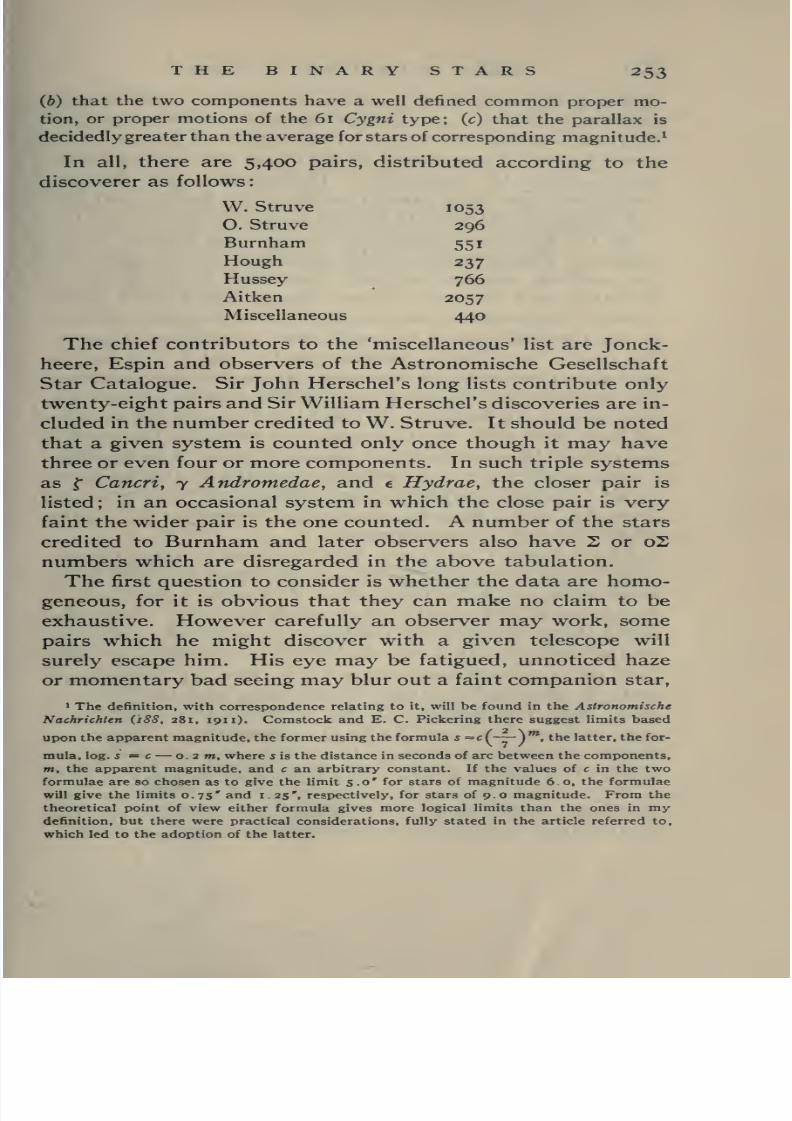
8/2/2019 The Binary Stars 1918
http://slidepdf.com/reader/full/the-binary-stars-1918 283/349
THE BINARY STARS 253
(b) that the two components have a well defined common proper mo-
tion, or proper motions of the 61 Cygni type; (c) that the parallax is
decidedly greater than the average for stars of corresponding magnitude.*
In all, there are 5,400 pairs, distributed according to the
discoverer as follows
W. Struve 1053
0. Struve 296
Burnham 551
Hough 237
Hussey 766Aitken 2057
Miscellaneous 440
The chief contributors to the 'miscellaneous' list are Jonck-
heere, Espin and observers of the Astronomische Gesellschaft
Star Catalogue. Sir John Herschel's long lists contribute only
twenty-eight pairs and Sir William Herschel's discoveries are in-
cluded in the number credited to W. Struve. It should be noted
that a given system is counted only once though it may have
three or even four or more components. In such triple systems
as ^ Cancri, 7 Andromedae, and € Hydrae, the closer pair is
listed ; in an occasional system in which the close pair is very
faint the wider pair is the one counted. A number of the stars
credited to Burnham and later observers also have S or oS
numbers which are disregarded in the above tabulation.The first question to consider is whether the data are homo-
geneous, for it is obvious that they can make no claim to be
exhaustive. However carefully an observer may work, some
pairs which he might discover with a given telescope will
surely escape him. His eye may be fatigued, unnoticed haze
or momentary bad seeing may blur out a faint companion star,
>
The definition, with correspondence relating to it, will be found in the AstronomischeNachrichlen {188, 281, 1911). Comstock and E. C. Pickering there suggest limits based
upon the apparent magnitude, the former using the formula s=c (~z~) "*. the latter, the for-
mula, log. 5 — c— 0.2 m, where 5 is the distance in seconds of arc between the components,
m. the apparent magnitude, and c an arbitrary constant. If the values of c in the two
formulae are so chosen as to give the limit 5.0' for stars of magnitude 6. 0, the formulae
will give the limits 0.75' and 1.25', respectively, for stars of 90 magnitude. From the
theoretical point of view either formula gives more logical limits than the ones in mydefinition, but there were practical considerations, fully stated in the article referred to,
which led to the adoption of the latter.

8/2/2019 The Binary Stars 1918
http://slidepdf.com/reader/full/the-binary-stars-1918 284/349
254 THE BINARY STARS
or it may chance that at the date of examination the two com-
ponents are so nearly in conjunction as to be below the resolv-
ing power of the telescope. The number of known doublestars can only be regarded as the lower limit to the number
which might be discovered. Homogeneity was earnestly
sought for, care being taken to work only when in good phys-
ical condition and when the seeing was good, the practical test
being the power to recognize very close and difficult pairs at
a glance. But variations in the conditions are inevitable when
the working program requires years for its execution and
doubtless such variations have affected the present results.
Careful comparison, however, shows no discernible difference
in the thoroughness of the work done at different seasons of
the year or in different parts of the sky, and it may fairly be
said that the results of the survey represent the capacity of
the combination of telescope and observer under average good
atmospheric conditions at Mount Hamilton. If the work had
all been done with the thirty-six-inch refractor the resulting
data might be considered quite homogeneous. Unfortunately,
a considerable part of it, including practically the entire area
north of +60° declination, was done with the twelve-inch
telescope, and it becomes necessary to consider the relative
efficiency of the two instruments.
I have applied two tests : first, the comparison of the most
difficult pairs discovered with each instrument; second, the re-
examination with the thirty-six-inch of some 1,200 stars pre-
viously examined with the twelve-inch telescope. I find that,
under the usual observing conditions, a pair with nearly equal
components separated by only o. 15'', or a companion star as
faint as 14.5 magnitude and not less than 1.5" from its pri-
mary is practically certain of detection with the thirty-six-
inch; with the twelve-inch, the corresponding limits in the
two cases are 0.25* and 13 to 13.5 magnitude. Twelve new
double stars were added by the re-examination of the 1,200
stars. From these tests, taking into account the proportion
of the whole work done with the twelve-inch telescope, I con-
clude that about 250 pairs would have been added if the entire
northern sky had been surveyed with the thirty-six-inch.

8/2/2019 The Binary Stars 1918
http://slidepdf.com/reader/full/the-binary-stars-1918 285/349
THE BINARY STARS 255
According to Seeliger's count of the B. D. stars there are
100,979 as bright as 9.0 magnitude in the northern hemis-
phere. Of these, 5,400, or i in 18.7 on the average, have
actually been found to be double within the limits set above.
If we add only 200 pairs, the ratio becomes i : 18.03. Adefinite answer is thus given to my first question: "At least
one in every eighteen, on the average, of the stars in the northern
half of the sky which are as bright as g.o B. D. magnitude is a
close double star visible with the thirty-six-inch refractor." There
is no reason to doubt that the ratio is equally high in the south-
ern half of the sky.
TABLE I
The Distribution of Double Stars in Right Ascension and
Declination
oh 2h 4h 6h 8h loh I2h I4h I6h I8h 20h 22h
R.A. to to to to to to to to to to to to
ih 3»^ 5^ 7h Qh Ilh i3»» IS*^ I7h IQh 2lh 23h
Decl.
o-'-Q^ 6.3 6.3 7-4 6.0 6.0 5-9 5.5 6.4 5.4 6.0 5-3 4-9
10-19 5-4 5-4 6.4 TT 5 5 5 5 4 8 6.1 4 5 6.0 5 4 5 2
20-29 5-2
6.0
5.6
5.5
5-9 5.1
4-4
4
4
8
3
6
4
4
8
5
5
2
4
4.8
415
5
4 6.2 4
5
9
2
4
4
2
30-39 8
40-49 6.7
6.2A^FT
8.0
4-5
5-2
4
4
5
8
6
3
2
6
3
4
2
4
5.6
6.0
5
4
5
6
4.2
4-4 6
2
8
4
4
9
50-59 TT 9
60-69
J±503.8
714.2
2.9
3-5
4
3
3
I
4
2
4
6
2
2
6
8
4.1
2.2
3
3
6
4
414-9
5
5
3 6
^70-79 5-9 T80-89 (oh to 5h) 3.7
(6h tOllh) 3 3 (l2htOI7h) 3 4 (I8ht023h) 3 9
The figures give the percentages of double stars among stars to 9. o B. D.
magnitude; the average percentage for the whole northern sky is 5.35.
Table I exhibits the distribution of the 5,400 double stars in
right ascension and declination as compared with the distribu-
tion of the B. D. stars to 9.0 magnitude, the figures giving the
percentage of double stars in each area. There are obvious
irregularities in the table but no evidence of systematic differ-
ences that can be regarded as seasonal effects. The percentages
are as high in the sky areas surveyed in winter as in those sur-
veyed in summer. There is a falling off in the percentage in

8/2/2019 The Binary Stars 1918
http://slidepdf.com/reader/full/the-binary-stars-1918 286/349
256 THE BINARY STARS
the high declinations, especially in the regions well removed
from the Milky Way, which is doubtless due in part to the
fact that the area north of 60° was almost entirely surveyed
with the twelve-inch telescope. The broken line in the table
represents very roughly the position of the central line of the
Milky Way, and it will be noted that the percentages near
this line are, in general, above the average.
^The distribution with respect to the plane of the Milky Wayis more clearly brought out when the stars are tabulated ac-
cording to galactic latitude. This has been done in Tables II
and III, in the former of which the stars are divided in classes
according to magnitude and the latitudes into zones each 20°
TABLE II
The Distribution of Double Stars by Magnitude Classes and
Zones of Galactic Latitude
m m m m m mMag. to
6.5 6.6-7.0 7.1-7.5 7.6-8.0 8.1-8.5 8.6-9.0Total
Zone
I 19 13 14 29 40 84 199
II 43 28 50 68 114 193 496
III 60 43 56 79 148 254 640
IV 96 54 81 132 232 401 996
V121 88
133 249 376 6531,620
VI 84 51 81 134 221 395 966
VII 28 23 18 54 90 154 367
VIII 7 6 5 12 31 55 116
Total 458 306 438 757 1,252 2,189 5,400
wide, beginning at the north galactic pole. Zone V therefore
includes the area from +10° to —10° galactic latitude, and
Zone IX, which ends at the south galactic pole and lies entirely
below the equator, is not represented. As was to be expected,
the numbers in every column of this table are largest in Zone Vand fall to minima in Zones I and VIII. The question is
whether this condensation toward the Milky Way is greater
than that of all the stars. Table III provides the answer.

8/2/2019 The Binary Stars 1918
http://slidepdf.com/reader/full/the-binary-stars-1918 287/349
THE BINARY STARS 257
I
•*^ CO
cS
6
1
Os
8 ^J
^
CO g
00
7)
d
»0 r^ r*! Qn CO t^ HH
fO rO CO vO
M.
Qn rj- Tj- 00 Q00 00 n 6tc T^ Tj- t>.
ov r^ t^00 CI Mt^ 10 10
H*
• 00
00
5 8.5 ^8c< CO ro vO
-+ t^ to
\0 -rt- ^H^
ON M c* Q^ ^ s=> ?l 8
ON f5 VOr^ lo Tf
«
00
1
»o cs
rO rO CO »0
ON »0rO J>- 10
fO <S
d^ rjr
C4 roTj-
Tl- 10 t^
M ro1^ 00 r^
r^ ^ COHH
10 d
vO 00 CM Cf> ON1^ N ->
dPQ
00 t^ Ov 10HH a\ a. vo10 Ti- 10 r^ 00 Tl- CO
>*
r^
^
C/3
d
-^ "*
re Tl- Tj- vO00 Tt- vONO "51- CO
'-'
dPQ
« 10 Tl- ONfO -rt- 10 00 QT^ rf 10 vO 5
t^ r^ ID
H
NO
2
in
d
10 vo a. QOn 10 00 00rO rj- n- l^
CI ON00 CO CO
dPQ
•1 <s ON10 1^ fD On Q10 10 vO t^
CI CI 00
ON lO Tj-
ts
S
c
N
^ ::^ > >>^

8/2/2019 The Binary Stars 1918
http://slidepdf.com/reader/full/the-binary-stars-1918 288/349
258 THE BINARY STARS
Since the zones are not of equal area, and since only the first
lies wholly in the northern hemisphere, the fairest comparison
is that afforded by the relative densities per square degree of
double stars and all stars of the corresponding magnitudes.
The double star densities were determined by dividing the
figures in Table II by the number of square degrees in each
zone area ; the figures were then reduced to a common standard
by making the density in each column unity in Zone V, the
Milky Way Zone. Seeliger has published corresponding data
for all of the B. D. stars and the two sets of values are entered
in Table III in the columns D. S. and B. D., respectively. It
is clear that the density curves of double stars rise to sharper
maxima in the Zone V than the corresponding curves of stars
in general do.
This fact is exhibited in a more striking manner if we tab-
ulate, as in Table IV, the percentages of double stars in five
areas, the Milky Way Zone, the 20° zone on either side of it
and the areas north of +30° and south of —30° galactic
latitude.
TABLE IV
Percentages of Double Stars
Galactic LatitudeB.D. Stars
to 9.0Double Stars
Percentage of
Double Stars
+90° to +30°
+30 +10
+ 10 —10
-10 -30
-30 -70
26,948
19,355
26,477
17,831
10,368
1,335
996
1,620
966
483
4-95
5.15
6.13
5.13
4.66
The increased percentage in Zone V must be accepted as
real. Table III shows that stars of all magnitude classes par-
ticipate in it, and an examination of my charts leads to the
conclusion that it cannot be an observing effect, for some areas
of all galactic latitudes were examined in summer, others in
winter; the area north of +60° declination, examined almost
exclusively with the twelve-inch, extends from —3° to +27°

8/2/2019 The Binary Stars 1918
http://slidepdf.com/reader/full/the-binary-stars-1918 289/349
THE BINARY STARS 259
C3
^ N rr> vO 00 6M Th w10 ro HH
::!"O
»-'
° S >lA
^ d b* n N NO t^ vo
Z H HH CO Td- 10 N>->
^ 2 ^%:;,sOn 00>«*• N
f_,IH
2Tf m d Tt- 00 ro -^ vO n ON M
Z i-i Tj- 10 t^ Tf t^ (S •"•
^ ^^P5S 8M NO
^ ^ NO CNJ
^
1-1
fO Tj- 6 10 10 M M .^ M C< On
Z i-i vO vo •-» vD CO
^ r< 00 10
MNO «
C4 fO 6 (^ HH M fO fO •^ (N< C<
Z CO VO fO rO rt- rj- wl-l HH (S
».Q vO 00 rf QHH fo Ti- t^ 5
rj- 00
M _
^ t^ W
10'
cs d rj- vO »0 •* 10 NO C<
z (S 10 vO -^ to HH
"
».Q« CO Tj- t^ 5
M
10 00 00
M _^^ NO W
'
d 10 vO "-I ^ On M Th
Z CS 10 ON fO 00 1-1 10 I-.
"
M l^ Qi-H CO CO 10
10 NO
fe^ 10 M
^d d i-i n a\ >o vo r« t^ 00
Z CO ON On t^ 10 i^ I-.
^Q tH vO vD 00 Pi-i M CO »0
Tt f 00
_
^ NO M
10
d d 11 11 10 00 t^ M CO
Z Tt CO M 00 t4- 00 COl-l HH C< CO W
1^
Q
^ n: s > >>^

8/2/2019 The Binary Stars 1918
http://slidepdf.com/reader/full/the-binary-stars-1918 290/349
26o THE BINARY STARS
galactic latitude and the areas of high galactic latitude, both
north and south, were examined mainly with the thirty-six-
inch refractor. We may therefore say that close visual double
stars are relatively more numerous in the Milky Way than else-
where in the sky.
Since the stellar system quite certainly extends to a much
greater distance in the plane of the Milky Way than at right
angles to it, the natural inquiry is whether the increased double
star density in the Milky Way is not merely a perspective
effect. If this were the case it would seem that we might
expect a relatively higher percentage of very close pairs in
Zone V than of pairs of moderate separation. Table V, how-
ever, in which the 5,400 pairs are grouped according to galactic
latitude and angular separation, shows that the percentage
increase toward Zone V is as great for stars with angular dis-
tances of from 2" to 5" as for stars under i".
Let us consider next the relation between the angular sep-
aration and magnitude. This is shown in Table VI where thestars are arranged with these qualities as arguments. The
sums of the numbers in the first two columns of the table are
entered in the third, thence the numbers are given for uniform
steps in angular distance to the final column. Every line of
columns three to seven exhibits a marked increase in the num-
ber of pairs as the angular distance diminishes.
This is still more clearly brought out when the figures in
these five columns are expressed as percentages of the total
number of stars under 5" separation in each magnitude class.
Now it is generally believed that stars of a given magnitude,
for example from 8.6 to 9.0, are approximately at the same
distance from us, on the average. Hence the observed increase
in the number of pairs as the angular distance diminishes is
not a mere perspective effect, but represents a real increase
in the number of pairs as the orbital dimensions diminish. The
uniformity of the percentages in each column in the lower
division of the table and the fair agreement between the ratios
of the figures in each line of the first two columns in the upper
division both argue that the Lick Observatory survey was as
thorough for the fainter stars as for the brighter ones. This

8/2/2019 The Binary Stars 1918
http://slidepdf.com/reader/full/the-binary-stars-1918 291/349
THE BINARY STARS 261
was to be expected, for with the thirty-six-inch refractor a
close and difficult double of magnitude eight to nine is as
readily seen as a similar pair of brighter magnitude; in fact,
I find that 123 of the 379 pairs with angular separation of
TABLE VI
The Distribution of Double Stars by Angular Distance
and Magnitude
to
O.SI' 0.00' 1. 01' 2.01' 3.01' 4.01' 5.01'
Dist. to to to to to to and0.50'
I. 00' 1 .00' 2.00' 3.00' 4.00' 5 00' over
Mag.
^ 6.5 75 63 138 83 62 41 31 996 . 6-7 . 82 52 •134 59 42 40 21 14
7I-7-5 103 67 170 99 64 48 31 29
7.6-8.0 178 132 310 164 107 85 63 26
8.1-8.5 310 223 533 285 173 128 III 21
8.6-9.0 508 413 921 532 317 217 191 II
Totals 1,256 954 2,206 1,222 765 559 448 200
Percentages
^ 6.5 39 23 17 12 9 100
6 . 6-7 . 45 20 14 14 7 100
71-75 41 24 16 12 7 100
7.6-8.0 42 22 15 12 9 100
8.1-8.5 43 23 14 II 9 100
8.6-9.0 42 25 14 10 9 100
Totals 42 23 15 II 9 100
0.25" or less, and385
of the877
pairs with angular separation
between 0.26" and 0.50" discovered in that survey are of
B. D. magnitude between 8.6 and 9.0.
These statements are of significance also in connection with
the figures exhibited in Table VII which shows the percentage
of double stars of each magnitude class. The high percentage
in the first line is partly due to the relatively large number of

8/2/2019 The Binary Stars 1918
http://slidepdf.com/reader/full/the-binary-stars-1918 292/349
262 THE BINARY STARS
bright double stars wider than 5.0". If this number is reduced
to the same order as that of the wider pairs for the other
magnitude classes, the percentage becomes 9.1.
TABLE VII
Percentage of Double Stars hy Magnitude Classes
Magnitude B.D. Stars Double StarsPercentage of
Double Stars
to6.5 4,120 458
II.
6.6-7.0 3.887 306 7-9
7.1-7-5 6,054 438 7.2
7.6-8.0 11,168 758 6.8
8.1-8.5 22,898 1,251 5-5
8.6-9.0 52,852 2,189 4.1
In view of what has been said above it is impossible to
attribute the disparity in the percentage of double stars amongthe brighter and fainter stars to incompleteness of the data,
and this becomes even more apparent when we recall that the
distance limit adopted (5.0") is the same for the stars in the
last magnitude class as for the stars as bright as 6.0. If the
adopted limit were a function of the magnitude, like those
suggested by Comstock and Pickering,^ and the value 5.0"
were retained for stars of 6.0 magnitude, we would have prac-
tically the same percentages in the first two lines of Table VII,
and diminished values in the following ones, the final percen-
tage (for stars 8.6 to 9.0) being only half its present
value.
The very high percentage of spectroscopic binary systems
among stars as bright as 5.5 magnitude may or may not be
significant in this connection, for we do not yet know whetherthat percentage will hold among the fainter stars, but on the
evidence before us we may venture the suggestion that per-
haps the stars of larger mass, and hence presumably greater
luminosity, are the ones which have developed into binary
systems.
* See footnote, page 253.

8/2/2019 The Binary Stars 1918
http://slidepdf.com/reader/full/the-binary-stars-1918 293/349
THE BINARY STARS 263
The stars have been grouped in the foregoing tables without
regard to their spectral class. We hiive now to see whether
any of the results obtained vary with the star's spectrum. In
June of the present year (191 7) Director E. C. Pickering and
Miss Annie J. Cannon, of the Harvard College Observatory,
generously permitted me to compare my list of double stars
with the manuscript of the New Draper Catalogue of Stellar
Spectra, which contains the spectral classification of over
200,000 stars. It is due to their great kindness, for which I
cannot adequately express my thanks, that I am able to present
the results which follow. The comparison with the NewDraper Catalogue has provided the spectral classification for
3,919 of the 5,400 visual double stars in the northern sky. Of
the remaining 1,481 stars only 15 are as bright as 8.0 magni-
tude (and about half of those were inadvertently omitted
from the list I took to Cambridge), 218 lie between 8.1 and
8.5, and 1 ,248 between 8.
6 and 9.
o magnitudes. Practically,
then, the data as to spectral class are complete for stars to
8.0, nearly complete for stars to 8.5, but less than half com-
plete for the stars between 8.6 and 9.0 B. D. magnitude.
The New Draper Catalogue is based upon objective prism
spectra and therefore, in general, ddes not record separately
the spectra of the components of such double stars as are
considered here. The spectrum for these is either the spec-
trum of the bright component, or, if the magnitudes are nearly
equal, a blend of the spectra of the tw^o components. A very
large number of the closer double stars have components
which differ but little in brightness, and it has long been
known that such pairs exhibit little or no color contrast.
Indeed, Struve, in his discussion of the stars in the Mensurae
Micrometricae showed that the color contrast between the
components of a double star was a function of their difference
of magnitude, and Lewis and other writers have extended his
researches. In my own observing I have noted the components
of hundreds of pairs of nearly equal magnitude as being of the
same color. I may add that although my eyes are entirely
normal as regards color perception I have never been able to
see such violent contrasts in any pair of 'colored stars' as are

8/2/2019 The Binary Stars 1918
http://slidepdf.com/reader/full/the-binary-stars-1918 294/349
266 THE BINARY STARS
scopic binaries evidently show a marked preference for the
early spectral classes from Bo to Ao, the visual binaries for
the classes from Ao to Ko. The maxima in certain of the sub-classes such as Ao and Ko are apparently real but probably
without special significance. The most unexpected feature of
the table is that the number of spectroscopic binaries of the
M sub-classes is relatively much greater than that of the
visual binaries.
To study the relations of these groupings to those of the
stars in general, I have combined the sub-classes into six larger
classes, using the Harvard system, which is indicated by the
heavy vertical rules in Table VIII, and have compared the
results with Pickering's tabulation of the stars in the Revised
Harvard Photometry.
TABLE IX
The Spectral Classes of the Binary Stars and of the Stars in the
Revised Harvard Photometry
Numbers
B A F G K M All
Vis. Bin. (all) 157 1,251 532 1,093 837 49 3,919
Vis. Bin. (to 6.5) 59 142 65 83 93 18 460
Spec. Bin. 198 161 61 71 95 19 605
R.H.P. Stars. 822 2,755 1,097 932 2,531 636 8,773
Percentages
Vis. Bin. (all) 4 32 14 28 21 I 100
Vis. Bin. (to 6.5) 13 31 14 18 20 4 100
Spec. Bin. 33 26 10 12 16 3 100
R.H.P. Stars. 9 21 13 II 29 7 100
V. B. (all) -H.P.
V.B. (6.5) -H.P.
Sp. B. -H.P.
-5 + 1 + 1 + 17 -8 -6
+4 + 1 + 7 -9 -3
+24 -5 -3 + I -13 -4
The numbers are not strictly homogeneous even for the Re-
vised Harvard Photometry stars and the spectroscopic binaries,

8/2/2019 The Binary Stars 1918
http://slidepdf.com/reader/full/the-binary-stars-1918 295/349
THE BINARY STARS 267
but are sufficiently so to permit comparison. To make the data
for the visual binaries more, directly comparable with the rest,
I have given separately the numbers for the systems as bright
as 6.5 magnitude B. D. The upper part of Table IX records
the actual numbers of the stars of each category and of each
spectral class; the lower part, the percentages and the excess
or defect of each percentage when compared with that of the
Revised Harvard Photometry stars. The figures in the last two
lines may be affected to a certain degree by the lack of strict
homogeneity in the data, but they certainly place beyondquestion the fact that spectroscopic binaries as bright as 5.5
magnitude are far more numerous among Class B stars than
among stars of other spectral classes, and that the visual
binaries as bright as 6.5 magnitude are in excess among Class
G stars and least numerous among stars of Classes K and M.
The discovery of spectroscopic binary stars is quite inde-
pendent of the distance of the system, for the displacement of
the lines in the spectrum (disregarding variations in the physi-
cal condition of the star) depends simply upon the velocity of
the light source in the line of sight. The observed or angular
separation of a visual binary, on the other hand, is a function
of its distance from us, and it is necessary to consider whether
this fact may not seriously influence the distribution shown
in the table, for many different recent investigations have led
astronomers to believe that stars of Classes F and G are, on
the average, the nearest, those of Classes B and M the most
remote. It is not easy to estimate the effect of this factor.
Certainly the 5" limit imposed in collecting the data does not
favor the Class G stars at the expense of those of Classes B
and M, for it is clear that of two systems of the same linear
dimensions the more distant one might fall within the limit
whereas the nearer one might be excluded by it. The more
distant pair might, it is true, fall below the resolving power
of the telescope while the nearer pair would be well enough
separated to be discovered, but this would not account for
the fact that the percentage of visual binaries (to 6.5 magni-
tude) is greater among the Class B stars than among those of
Class F or Class K. Admitting the uncertainties arising from

8/2/2019 The Binary Stars 1918
http://slidepdf.com/reader/full/the-binary-stars-1918 296/349
268 THE BINARY STARS
the unknown distances of the double stars and from errors
in the classification, I am still of. the opinion that the last two
lines of the table give a fair qualitative representation of the
true distribution with respect to spectrum of the visual
binaries among stars as bright as 6.5 magnitude, as well as of
the spectroscopic binaries.
The percentages for the visual binaries to 9.0 magnitude
will quite certainly be modified when we can compare the
TABLE X
The Distribution of Double Stars by Spectral Class
and Galactic Latitude
Un- B.D.B A F G K M
known Stars
I I II 24 51 52 2 58 4,276
II I 45 50 159 121 3 117 8,798
III 4 87 78 170 129 5 167 13,874
IV 16 260 95 186 148 8 283 19,355
V 109 542 118 202 168 14 467 26,477
VI 22 247 lOI 183 122 II 280 17,831
VII 3 48 48 105 74 5 84 7,998
VIII I II 18 37 23 I 25 2,370
Sums 157 1,251 532 1,093 837 49 1,481 100,979
Percentages
I I 2 20 25 31 14 12 16
II I 8 42 79 72 21 25 33
III 4 16 66 84 77 36 36 52
IV 15 48 81 92 88 57 61 73
V 100 100 100 100 100 100 100 100
VI 20 46 86 91 73 79 60 67
VII 3 9 41 52 44 36 18 30
VIII ^ 2 15 18 14 7 5 9
3,919 double star spectra with the spectra of all the stars in
the New Draper Catalogue. It may be pointed out also that
the 9.0 magnitude limit may operate here to favor Classes
B and A at the expense of Class K, for the former classes con-

8/2/2019 The Binary Stars 1918
http://slidepdf.com/reader/full/the-binary-stars-1918 297/349
THE BINARY STARS 269
tain a high percentage of stars intrinsically bright, the latter
a considerable percentage of 'dwarfs'.
Table X is arranged to show the distribution of the visual
binaries of different spectral classes with respect to the galactic
plane. I have placed the systems for which the spectral class
is unknown in the seventh column of the table and in the final
column have added Seeliger's count of the B. D. stars to 9.0
magnitude.
Visual binaries of every spectral class increase in number as
we approach the Milky Way, but only in Classes B, A and M(and in the systems of unknown spectrum) is the increase
TABLE XI
The Distribution of the Spectroscopic Binaries by Spectral Class
and Galactic Latitude
B A F G K M All
I 7 I 4 12
II 3 21 5 4 3 I 37
III 6 17 6 II 7 ' 48
IV 31 27 9 4 19 3 93
V 76 44 12 25 20 9 186
VI 63 26 17 16 20 3 145
VII 10 II 7 6 17 I 52
VIII 7 8 3 I 8 27
IX 2 I I I 5
Sums 198 161 61 71 95 19 605
greater than that shown by the B. D. stars to 9.0 as a whole.
The fact brought out in Tables III and IV that visual double
stars are relatively more numerous in the Milky Way than
elsewhere in the sky must therefore be due to the systems of
these classes, and especially, in view of the actual numbers,
to those of Class A and of unknown spectral class. Possibly
the latter are also largely of Class A. The strong concentra-
tion of the Class M stars toward the Galaxy is due entirely to

8/2/2019 The Binary Stars 1918
http://slidepdf.com/reader/full/the-binary-stars-1918 298/349
270 THE BINARY STARS
the thirteen stars of Sub-classes Ma and Mb. These fall in
Zones IV, V and VI in the numbers 3, 7 and 3, respectively.
The thirty-six stars of Sub-class K5 are as uniformly distrib-
uted as those of Class K (G5 to K2).
Table XI, exhibiting the distribution in galactic latitude of
the 605 spectroscopic binaries, shows a similar increase in the
TABLE XII
The Distribution of Double Stars by Magnitude
and Spectral Class
B A F G K MB.D.
Stars
To 6 . mag.
6.1-6.5
38
21
85
57
38
27
53
30
61
32
39
64,120
6.6-7.0 15 109 51 59 72 I 3,887
7.1-7-5 20 162 64 104 82 3 6,054
7.6-8.0 30 232 126 209 137 8 11,168
8.1-8.5 21 308 128 347 220 9 22,898
Sums 145 953 434 802 604 66 48,127
Numbers Expressing Relative Frequency
To 6.5 mag.
6.6-7.0
71-7.
7.6-8.0
8.1-8.5
87.4
23.6
20.4
16.5
5-5
14.
II. 4
II.
8-5
5-5
15-3
12.8
10.3
II .0
5-5
12.9
10.6
7-8
7.0
5-5
149
4
6
9
5
(II. I)
( 7.9)
( 7-2)
( 6.8)
( 5.5)
numbers in all spectral classes as we approach the Milky Way.
In this case we are considering the entire sky and may there-
fore bring out the effect of the Milky Way more strikingly bydividing the sky into three zones by lines at =^30° galactic
latitude. The central zone contains half the sky area and it is
seen that six-sevenths of the Class B systems, four-fifths of the
Class M, but only five-eighths of those of each of the remaining
classes fall within this half. Class B stars as a whole are rela-
tively more numerous in the Milky Way than elsewhere in the

8/2/2019 The Binary Stars 1918
http://slidepdf.com/reader/full/the-binary-stars-1918 299/349
THE BINARY STARS 271
sky in a ratio as great as that shown by the spectroscopic
binaries of this class, but stars of Class M are quite uniformly
distributed over the sky. That so higha percentage both of
the visual and of the spectroscopic binaries of this class are
in or near the Milky Way is somewhat surprising.
In Table VII it was shown that the percentage of double
stars is higher among the bright than among the faint stars.
To see whether this holds for all spectral classes, I have ar-
ranged Table XII.
The spectral class is known for less than half of the double
stars of magnitude 8.6 to 9.0 and this group is therefore
omitted from the table. The upper part of the table gives the
actual numbers of pairs of the various classes; the lower part
was formed as follows : The numbers in each row in the upper
part (after combining the first two lines) were divided by the
number of B. D. stars of corresponding magnitude. The
figures in the six resulting columns were then made com-
parable by introducing factors to make those in the bottom
row all equal to 5.5, the percentage of double stars among
stars of magnitude 8.1-8.6 in Table VII.
The comparison of the first six columns in this part of the
table with the figures in parenthesis in the last column, which
are repeated from Table VII, shows that double stars of every
spectral class except G contribute to the increase in the per-
centage of pairs as the apparent brightness increases. Theexcess of double stars brighter than 6.5 magnitude in Classes
B and M is very striking, but the actual numbers as given in
the upper part of the table show that in the other magnitude
grades double stars of Classes A, F and K are more effective
in producing the observed progression.
I have prepared tables similar to Table VI for the double
stars of each spectral class, but for the sake of brevity I shall
give only their summary.
In forming the percentages I have, as in Table VI, omitted
the pairs wider than 5 . o". It is apparent that the progression
of numbers with decreasing angular distance begins to fall off
with Class K, and is still less appreciable in Class M. The
individual tables of which XIII is the summary indicate that

8/2/2019 The Binary Stars 1918
http://slidepdf.com/reader/full/the-binary-stars-1918 300/349
272 THE BINARY STARS
the distribution by magnitude shown in Table VI holds in
Classes A, F, and G, and also in Classes B and K, though in
these it is less marked for the brighter stars. It does not hold
for the small group of Class M stars.
TABLE XIII
The Distribution of 3,QIQ Visual Binaries by Spectral Class
and Angular Separation
o.oo'
to
I .00*
I .01'
to
2.00'
2.01'
to
300'
3.01'
to
4.00'
4.01'
to
500'
over
5.00'
Class B 60 33 29 10 9 16
A 540 283 158 122 88 60
F 222 115 55 74 44 22
G 489 236 143 106 82 37
K 273 187 144 108 78 47
M 12 10 8 5 6 8
Percentages
B 43 23 21 7 6 100
A 45 24 13 10 8 100
F 43 23 II 14 9 100
G 46 22 14 10 8 100
K 34 24 18 14 10 100
M 29 25 29 12 15 100
A large percentage of the visual binary stars have measur-
able proper motions and are therefore among the stars rela-
tively near us (say within a radius of 500 light-years) those
in which rapid orbital motion has been observed being, on the
average, the nearer ones. No investigation of their actual
distribution in space, however, has so far been published ; nor
has the spatial distribution of the spectroscopic binaries as a
whole been investigated.
Hertzsprung, however, has studied the distribution of the
Cepheid binaries, and Russell and Shapley that of the eclipsing

8/2/2019 The Binary Stars 1918
http://slidepdf.com/reader/full/the-binary-stars-1918 301/349
THE BINARY STARS 273
binaries. In each case it is found that the majority of the
stars investigated (sixty-eight Cepheids and ninety ecHpsing
systems) lie within a region bounded by planes drawn parallel
to, and comparatively close to the plane of the Milky Way,
and that within this region they are scattered over a vast
extent of space. In the case of the Cepheids the median plane
of the region passes about 123 light-years south of the Sun, the
mean distance of a system from this plane is 296 light-years,
while their distances from a central point defined by a perpen-
dicular from the Sun upon the median plane range from about
500 to nearly 10,000 light-years. The median plane for the
eclipsing binaries lies about 100 light-years south of the Sun,
a considerable majority of the systems, including nearly all
those of short period, lie within 500 light-years from this plane
and all of the others within 1,000 light-years; whereas their
distances parallel to the plane from a central point defined as
before range up to at least 8,000 light-years provided that
light suffers no absorption in its passage through space. As-
suming what the authors consider "a plausible amount of
absorption of light in space," the limits are cut down to 4,000
light-years.
It is almost unnecessary to add that both of these conclu-
sions, however reasonable they may be regarded, rest upon
more or less speculative hypotheses and are not to be con-
sidered as definitely established.

8/2/2019 The Binary Stars 1918
http://slidepdf.com/reader/full/the-binary-stars-1918 302/349
CHAPTER XI
THE ORIGIN OF THE BINARY STARS
Any theory of the origin of the binary stars must take
account of the facts of observation which have been outHned
in the three preceding chapters. Chief among these are the
following
1. The great number of the binary systems. On the average, at
least one star in eighteen of those as bright as 9 . o magnitude is a
binary visible in our telescopes; at least one in every three or four of
those as bright as 5.5 magnitude is a binary revealed by the spectro-
graph. These are minimum values. Our knowledge of the fainter
stars is very incomplete, but on the evidence before us we may safely
say that one-third, probably two-fifths, of the stars are binary systems;some astronomers, indeed, are inclined to think that systems of the
type of our solar system may be the exception rather than the rule.
2. The considerable percentage of systems with three or more
components. It is well within the truth to say that one in twenty of
the known visual binaries has at least one additional member either
visible in the telescope or made known by the spectrograph, and many
systems are quadruple or still more complex. Evidence is also accum-
ulating to the effect that many of the purely spectrographic systems
are triple or multiple. It is a fact of undoubted significance that, as a
rule, triple systems, whether visual or spectroscopic, consist of a close
binary pair and a companion relatively distant.
3. The close correlation between the length of period, or size of
system, and the degree of ellipticity in the orbit. The visual binaries,
with orbit periods to be reckoned in tens of years, have average eccen-
tricity close to 0.5; the spectroscopic binaries, with periods to be
counted in days or fractions of a day, have average eccentricity of
about 0.2; and in each class the average eccentricity increases with
the average length of the period. We have, then, an unbroken pro-
gression or series of orbits from systems in which the two components
revolve in a fraction of a day in circular orbits and practically in
surface contact, to systems in which the components, separated by
hundreds of times the distance from the Earth to the Sun, revolve in

8/2/2019 The Binary Stars 1918
http://slidepdf.com/reader/full/the-binary-stars-1918 303/349
THE BINARY STARS 275
highly elliptic orbits in periods of hundreds, perhaps thousands of
years.
4. The correlation between length of period and spectral type.
The short period spectroscopic binaries are prevailingly of spectral
Class B; the longer period spectroscopic binaries are usually of much
later spectral class ; the visual binaries have few representatives among
stars of Class B and are most numerous among stars of Classes F and G.
5. The correlation between the relative brightness of the com-
ponents and their relative mass. When the two components are of
equal brightness they are of equal mass, so far as our investigations
have been able to go; in other systems the brighter star is, almost
without known exception, the more massive, but the range in mass is
far smaller than the range in brightness. No system is known in
which the two components have a mass-ratio as small as i /lo.
6. The relatively great mass of a binary system, taking the Sun as
standard. Among the spectroscopic binaries showing two spectra we
have found only one {d Aquilae) which has a minimum mass value less
than the Sun's; the other minimum values given in Table VIII of
Chapter VIII, range from one and one-half to thirty times the solar
mass. The average mass of the visual binaries for which the data are
really determinate is nearly twice that of the Sun, and only one system
is known (Krueger 60) in which the mass can with any probability be
said to be as small as half that of the Sun.
7. The spectroscopic binary of Class B is, on the average, fully
three times as massive as the binary of later spectral class. We have
no data for the mass of a visual binary of Class B.
8. A few systems are exceptions to the general rules. For example,the short period spectroscopic binaries of early spectral class with very
eccentric orbits; the long period spectroscopic binaries of late spectral
class, and the long period visual binaries with nearly circular orbits;
the occasional system in which the fainter star is apparently the more
massive.
This enumeration is not exhaustive; I have, for instance,
omitted the facts, brought out in my statistical study of thevisual binaries in the northern sky, that such systems are
somewhat more numerous, relatively, among the stars of the
Milky Way than among those remote from it; that the bi-
naries which cause this apparent concentration are chiefly of
spectral classes B, A, and M; that there are apparently more
binaries, relatively, among the brighter stars than among the

8/2/2019 The Binary Stars 1918
http://slidepdf.com/reader/full/the-binary-stars-1918 304/349
276 • THE BINARY STARS
fainter ones, to 9.0 magnitude; for some of these relations
may prove to have no physical significance but to arise from
the fact that our material necessarily consists of selected stars.
As it stands, however, the enumeration is ample to indicate
the difficulties attending any attempt to formulate a theory of
general applicability.
If we consider a single binary system, it is conceivable that
it might originate in any one of at least three different ways:
1. Two stars, hitherto independent, might approach each other
under such conditions that each would be swerved from its original
path and forced to revolve with the other in orbits about their commoncenter of gravity (Capture Theory).
2. A single star, in its primal nebulous stage, or possibly even later,
might divide into two, which would at first revolve in surface contact
(Fission Theory).
3. The material in the primal nebula might condense about two
nuclei separated by distances of the order of those now existing be-
tween the centers of the component stars (Independent NucleiTheory).
No one of these theories is entirely satisfactory when we
consider the binary stars as a whole, and this is sufficiently
demonstrated by the fact that each one of the three has its
advocates among able astronomers at the present time. Since
I have no new theory to advance I shall content myself with
an exposition of the principles involved in each of the three
and its apparent accordance or discordance with the facts of
observation.
What I have called the capture theory appears to have
been proposed originally by Dr. G. Johnston Stoney, in 1867.
On May 15 of that year he presented a paper to the Royal
Society of London On the Physical Constitution of the Sun and
Stars, the major portion of which is concerned with the Sun.
In Section 2 of Part II, however, he treats of multiple stars
and, distinctly stating that his deductions are "of necessity, a
speculation," argues that if two stars should be brought very
close to each other one of three things would happen. The
third is that "they would brush against one another, but not
to the extent of preventing the stars from getting clear again."
In this event his analysis indicates that the stars would there-

8/2/2019 The Binary Stars 1918
http://slidepdf.com/reader/full/the-binary-stars-1918 305/349
THE BINARY STARS 277
after move in elliptic orbits, but that their atmospheres would
become engaged at each periastron passage. Since the atmos-
phere of each star "is not a thing of uniformdensity," the
resistance would take the form of forces acting, some tan-
gentially, and some normally, to the stellar surfaces; the
former would tend to reduce the periastron distance, the latter
to increase it, and as one or the other dominated in a special
case, the two stars would ultimately "fall into one another" or
"gradually work themselves clear of one another." In the
latter event a double star would result.
Meanwhile, "the heat into which much of the vis viva of the
two components has been converted will dilate both to an
immense size, and thus enable the two stars gradually in suc-
cessive perihelion passages to climb, as it were, to the great
distance asunder, which we find in the few cases in which the
final perihelion distance can be rudely estimated, a length
comparable with the intervals between the more remote
planets and the Sun. During this process, the ellipticity of
the orbit is at each revolution decreasing; but if the stars
succeed in getting nearly clear of one another's atmospheres
before the whole ellipticity is exhausted, the atmospheres will
begin to shrink in the intervals between two perihelion pas-
sages more than they expand when the atmospheres get en-
gaged, and will thus complete the separation of the two stars.
When once this has taken place, a double star is permanently
established."
According to Stoney, then, the eccentricity of a system
decreases and its major axis increases up to the time when the
atmospheres of the two stars are completely disengaged even
at perihelion passage. The most favorable case for the
formation of a double star on this hypothesis is presented when
the original stars are of equal mass; and since no double starcan result unless the unequal pressure of the atmospheres in
their grazing collision has imparted to at least one of the two
"a swift motion of rotation," Stoney imagines that under
special conditions the rotational motion might become so great
as to exceed the cohesive strength of the star and there might
"result two or more fragments spinning violently," ultimately

8/2/2019 The Binary Stars 1918
http://slidepdf.com/reader/full/the-binary-stars-1918 306/349
278 THE BINARY STARSI
leading to the formation of triple systems like that of 7"
Andromedae.
I have given Stoney's theorysomewhat
in detailbecause the
fundamental principle in it, namely, that collisions of stars in
various degrees, central, partial, or grazing, might produce the
stellar systems as we now know them has frequently appeared
in later speculations on cosmogony. Professor A. W. Bickerton
has elaborated it into a complete theory of cosmic evolution;
it was regarded favorably by Lord Kelvin (so far as the binary
stars are concerned); it appears again in Arrhenius's book,
Worlds in the Making, and has quite recently been presented,
with apparent approval, by Moulton in his discussion of the
origin of binary stars in the revised edition of his text-book,
An Introduction to Astronomy.
Moulton analyzes the special case of two stars each equal to
the Sun in mass which, at a great distance apart, have a
relative velocity that is zero. Let them approach each other,
but assume that at the point of nearest approach they are as
far apart as the Earth is from the Sun ; their relative velocity
at that instant will be about thirty-seven miles per second.
Now, if they encounter no resistance to their motion, they will
simply swing round each other and then separate again, moving
along parabolic paths. If, however, one or both encounter
resistance "from outlying nebulous or planetesimal matter, or
from collision with a planet" their velocities will be reduced
and their orbits may be transformed into elongated ellipses.
Moulton states that, in the assumed case, if the resistance
reduces the velocity by 1/200 of its amount, or 0.185 miles
per second, the stars will, after their nearest approach, recede
to a distance of only 100 astronomical units, and that the
reduction of velocity will generate only as much heat as the
Sun radiates in about eight years, not enough to affect the
stars seriously. The eccentricity of their orbits will be about
0.98, their revolution period about 250 years. Collision with
a planet comparable to Jupiter in mass would suffice to bring
about the results described.
If no subsequent collisions occur, the two stars will continue
to move in very elongated ellipses about their common center

8/2/2019 The Binary Stars 1918
http://slidepdf.com/reader/full/the-binary-stars-1918 307/349

8/2/2019 The Binary Stars 1918
http://slidepdf.com/reader/full/the-binary-stars-1918 308/349
28o THE BINARY STARS
known." That is quite correct, but it is none the less possible
as a matter of statistical calculation to estimate the probable
frequency of stellar encounters, and thus to apply a numerical
test to the probability of the theory. Such a calculation has
recently been made (for a different purpose) by Professor
J. H. Jeans.i
Assume i,ooo million stars (perhaps ten times as many as
are visible with our greatest telescopes) to be distributed in
a space within a parallactic distance of o.ooi" from the Sun,
a space which corresponds to a sphere having a radius of 3,260
light-years. Their mean distance apart, if they are arranged
in cubical piling, is then 10^^'^ centimeters, or about 330,000
times the Earth's distance from the Sun. Under reasonable
assumptions as to masses and velocities, Jeans finds that "a
star is only likely to experience a non-transitory encounter
about once in 4 X 10^^ (40 million million) years." To put it
differently, only one star in every 4,000 will experience a non-transitory encounter in 10,000 million years. By a non-
transitory encounter is meant one which will produce serious
tidal deformations in one of the stars. If the stars are taken
equal to the Sun in mass and given a relative velocity of forty
kilometers per second, their separation at point of nearest
approach must be not greater than the radius of Jupiter's
orbit (aboutfive astronomical units) to
produce alasting
ornon-transitory encounter. Transitory encounters, encounters
in which the distance at point of nearest approach exceeds five
astronomical units, will naturally be more frequent, but, with
the data assumed, in 10,000 million years only about one star
in three will have another star approach within 200 astronom-
ical units of its center; that is, within seven times the distance
of Neptune from the Sun!
It is perhaps conceivable that a single encounter similar to
the one Moulton describes might occur, but it is quite incon-
ceivable that more than a very few should occur in any length
of time that may reasonably be assigned for the age of our
present stellar universe. Still more inconceivable is the sup-
1 The Motion of Tidally-distorted Masses, with Special Reference to Theories of Cos-
mogony. Mem. R. A. S., 72, Part I, 1917-
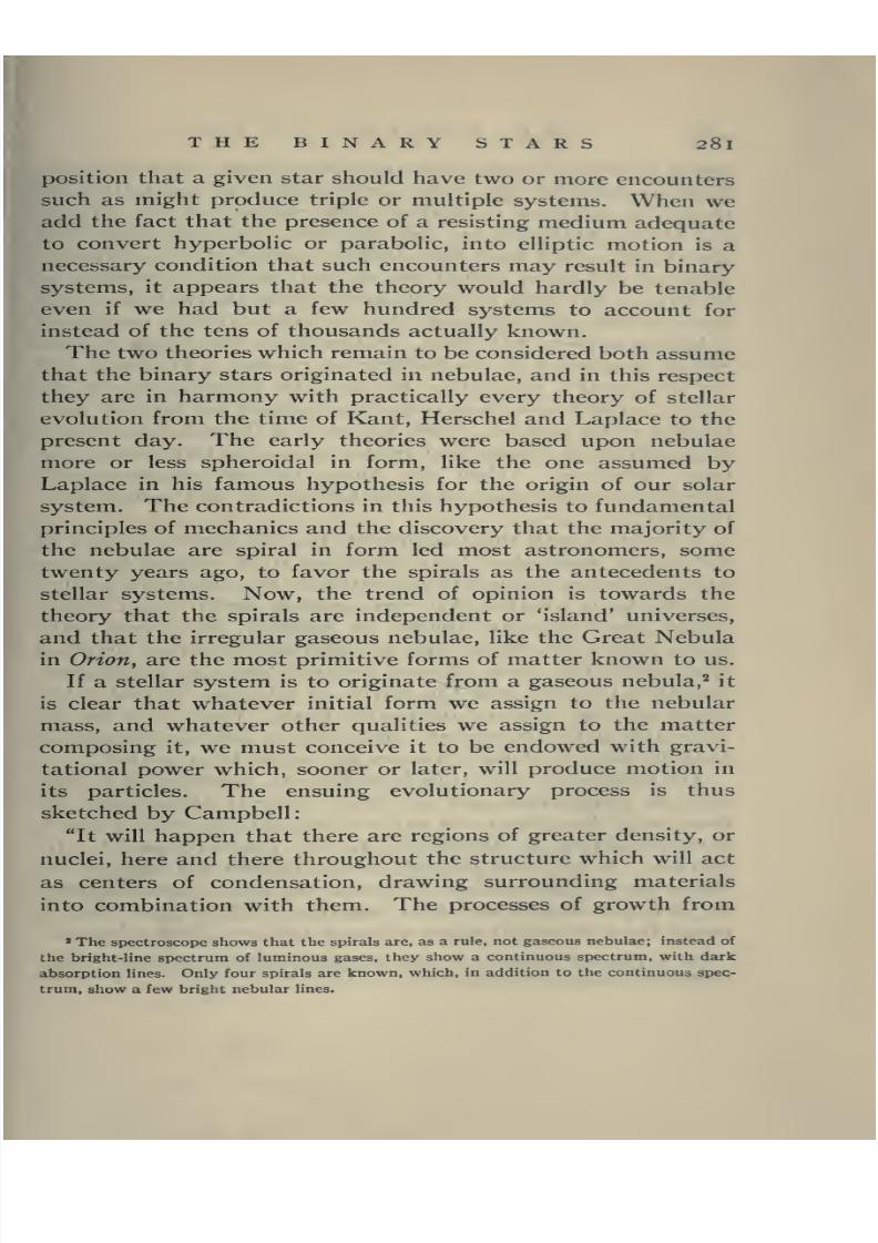
8/2/2019 The Binary Stars 1918
http://slidepdf.com/reader/full/the-binary-stars-1918 309/349
THE BINARY STARS 281
position that a given star should have two or more encounters
such as might produce triple or multiple systems. When we
add the fact that the presence of a resisting medium adequate
to convert hyperbolic or parabolic, into elliptic motion is a
necessary condition that such encounters may result in binary
systems, It appears that the theory would hardly be tenable
even if we had but a few hundred systems to account for
instead of the tens of thousands actually known.
The two theories which remain to be considered both assume
that the binary stars originated in nebulae, and in this respect
they are in harmony with practically every theory of stellar
evolution from the time of Kant, Herschel and Laplace to the
present day. The early theories were based upon nebulae
more or less spheroidal in form, like the one assumed by
Laplace in his famous hypothesis for the origin of our solar
system. The contradictions in this hypothesis to fundamental
principles of mechanics and the discovery that the majority of
the nebulae are spiral in form led most astronomers, some
twenty years ago, to favor the spirals as the antecedents to
stellar systems. Now, the trend of opinion is towards the
theory that the spirals are independent or 'island' universes,
and that the irregular gaseous nebulae, like the Great Nebula
in Orion, are the most primitive forms of matter known to us.
If a stellar system is to originate from a gaseous nebula,^ it
is clear that whatever initial form we assign to the nebular
mass, and whatever other qualities we assign to the matter
composing it, we must conceive it to be endowed with gravi-
tational power which, sooner or later, will produce motion in
its particles. The ensuing evolutionary process is thus
sketched by Campbell:
"It will happen that there are regions of greater density, ornuclei, here and there throughout the structure which will act
as centers of condensation, drawing surrounding materials
into combination with them. The processes of growth from
» The spectroscope shows that the spirals are, as a rule, not gaseous nebulae; instead of
the bright-line spectrum of luminous gases, they show a continuous spectrum, with dark
absorption lines. Only four spirals are known, which, in addition to the continuous spec-
trum, show a few bright nebular lines.

8/2/2019 The Binary Stars 1918
http://slidepdf.com/reader/full/the-binary-stars-1918 310/349
«82 THE BINARY STARS
nuclei originally small to volumes and masses ultimately stu-
pendous must be slow at first, relatively more rapid after the
masses have grown to moderate dimensions and the suppliesof outlying materials are still plentiful, and again slow after
the supplies shall have been largely exhausted. By virtue of
motions prevailing within the original nebular structure, or
because of inrushing materials which strike the central masses,
not centrally but obliquely, low rotations of the condensed
nebulous masses will occur. Stupendous quantities of heat
willbe
generated in the building-up process.This heat
will
radiate rapidly into space because the gaseous masses are
highly rarified and their radiating surfaces are large in pro-
portion to the masses. With loss of heat the nebulous masses
will contract in volume and gradually assume forms more and
more spherical. When the forms become approximately
spherical, the first stage of stellar life may be said to have been
reached." ^
If we start with the assumption that the binary systems as
well as the single stars have developed from nebulae by some
such process as Campbell has outlined, the question we have
to consider is whether they were formed directly by conden-
sation about separate nuclei, or whether, in a very early
stage, they were single stars or spheroidal nebulae, dividing
later under the stress of such internal forces as gravitation,
radiation pressure and the forces of rotation, or under the
strain of some external disrupting force. Each view has its
advocates and its opponents, and so far as strict mathematical
analysis goes, no definite answer has as yet been made.
The behavior of a rotating homogeneous incompressible fluid
mass in equilibrium and free from external disturbance has
been made the subject of a series of brilliant researches by such
mathematicians as Maclaurin, Jacobi, Poincare, and G. H.
Darwin. It has been possible, under certain assumptions, to
follow the transformations of form as the mass contracts under
its own gravitation and heat radiation and to show that it
passes from the initial sphere through a succession of spheroids,
» W. W. Campbell, 'The Evolution of the Stars and the Formation of the Earth'. Scien-
tific Monthly, September-Decamber, 191 S-

8/2/2019 The Binary Stars 1918
http://slidepdf.com/reader/full/the-binary-stars-1918 311/349
THE BINARY STARS 283
ellipsoids and pear-shaped figures till a stage is reached where
it seems certain that the next transformation will be a rupture
into two masses. The analysis becomes too complicated to
permit this step to be demonstrated mathematically.
The stars and the antecedent nebulae are not homogeneous
nor incompressible, but it has been argued, first, I believe, by
Dr. T. J. J. See, later by Darwin and others, that a nebula
might none the less pass through a series of similar changes
and ultimately form a double star. Darwin has shown that
the two portions must have fairly comparable masses if the
system, immediately after the rupture, is to be a stable one.
Once formed, with components revolving in surface contact
and in orbits practically circular, the agency of tidal forces is
invoked to produce increase in the ellipticity of the orbit and
in the length of the major axis.
The potency of tidal friction, within limits to be noted later,
is undeniable, and the whole theory is made exceedinglyplausible by its apparent ability to explain many of the facts
of observation. Thus, according to the classical theory of
stellar evolution, the stars of spectral Classes Oe and B are the
'young' stars; those of Classes A, F, G, and K, progressively
older, the red stars of Class M, the 'old' stars, age being mea-
sured not in duration of time but by the stage of development
reached. Now, as we have seen, the spectroscopic binaries
which, on the average, have the shortest periods and orbits
most nearly circular, are young stars; spectroscopic binaries of
long period and high eccentricity belong, on the average, to
the later spectral classes; they are old stars. Visual binaries
of known period are wanting among stars of very early or very
late spectral class. Campbell, who favors the fission theory,
argues that the binaries of very early type have components
too close together to be separately visible, while those of very
late spectral class have their components so far apart that the
revolution periods are exceedingly long. He also thinks that,
in many red binary pairs, the fainter component may have
become so faint as to be no longer visible.
Russell finds further support for the fission theory in the
numerous triple and quadruple systems. His analysis leads

8/2/2019 The Binary Stars 1918
http://slidepdf.com/reader/full/the-binary-stars-1918 312/349
284 THE BINARY STARS
him to conclude that, with a distribution of masses such as is
actually found in double star systems, if further division occurs,
the resulting multiple system must consist of a (relatively)
wide pair one or both of whose components are themselves
more closely double, the distance separating the components
of the closer pair or pairs being "less than about one-fifth that
of the wider pair—usually much less." He finds support for
his conclusions in his discussion of the distance ratios in the
known triple and quadruple systems.
The alternative theory, that double stars had their origin in
separate nuclei in the parent nebula, was first suggested a
century ago by Laplace. In Note VII to his Systbme du
Monde he remarks:
"Such groups (as the Pleiades) are a necessary result of the
condensation of nebulae with several nuclei, for it is plain that
the nebulous matter being constantly attracted by these dif-
ferent nuclei must finally form a group of stars like the Pleiades.
The condensation of nebulae with two nuclei will form stars in
very close proximity, which will turn one around the other,
similar to those double stars whose relative motions have
already been determined." ^
Laplace's theory is quite generally accepted for those wide
and irregular groups, like B Ononis, "for which the fission theory
gives no explanation," and it is not without its adherents evenfor the usual type of binary system. The modern writer who
has adopted it most explicitly is the very man who first for-
mulated the fission theory, Dr. See. His discussion of the
binary stars in the second volume of his Researches on the
Evolution of the Stellar Systems is devoted more particularly to
the development of the systems after their initial formation but
on page 232 we find the statement, "Itis
evident. . .
thatthe resulting mass-ratio in a system depends on the supply of
nebulosity and the original nuclei already begun and slowly
developing in the nebula while it was still of vast extent and
great tenuity;" and, on page 584, the even more definite state-
ment, "When a double star had been formed in the usual
* See Essays in Astronomy, p. soi. (Edited by E. S. Holden; D. Appleton & Co.,
1900).

8/2/2019 The Binary Stars 1918
http://slidepdf.com/reader/full/the-binary-stars-1918 313/349
THE BINARY STARS 285
way (Italics mine) by the growth of separate centers in a widely
diffused nebula ..."Moulton, as we have seen, favors the theory that binaries
arose from entangling encounters of independent stars, but as
between the two theories now under discussion, remarks"
. . .we are led to believe that if binaries and multiple
stars of several members have developed from nebulas, the
nebulas must originally have had well-defined nuclei. The
photographs of many nebulas support this conclusion." And
Russell, while advocating the fission theory, admits that "The
close pairs, almost in contact, revealed to us among the variable
stars may be accounted for on either theory. The apparently
universal fact that the components of a binary are comparable
in mass is what might be expected as a consequence of the
fission theory, but would probably have to be a postulate of
the other."
Now it is obvious that the separate-nuclei theory affords
sufficient latitude for the explanation of any conceivable
system. We may imagine the two nuclei to be so remote from
each other originally that their initial approach will be prac-
tically along the paths of parabolas and then invoke the action
of a resisting medium to convert the motion first into that in
an elongated ellipse and later into ellipses of ever smaller
eccentricity and major axes; or we may imagine them placedso near each other that their relative motion is at first in small
circular orbits which are afterward enlarged and made more
eccentric by the action of tidal forces; and, in fact, this,
crudely put, is the argument which See makes. That is, he
considers that both of these opposing forces are actually effec-
tive in producing the binary systems as we now see them, one
or the other becoming dominant in a particular system.
The fundamental objection to the separate nuclei theory is
that we really do not explain anything; to use Moulton's
words, "we only push by an assumption the problem of ex-
plaining the binary systems a little farther back into the
unknown."
Russell's specific objection, based upon his study of the
triple and quadruple systems is also of great force. Why

8/2/2019 The Binary Stars 1918
http://slidepdf.com/reader/full/the-binary-stars-1918 314/349
286 THE BINARY STARS
should these systems almost invariably consist of a compara-
tively close binary pair attended by a third star or by another
close binary pair at a distance relatively great? As Russell
says, "Not only is there no apparent reason for it, but if we
try to retrace in imagination the history of such a system,
through stages of greater and greater diffusion as we penetrate
farther into the past (keeping in mind that the moment of
momentum of the whole system must remain constant), it is
hard to form any idea of the history of the nuclei which will
finally form a close and rapidly revolving pair, attended by adistant companion."
All things considered, the theory which has most in its favor
is the fission theory, though it must be admitted that there are
very serious difficulties about accepting it unreservedly.
These relate, first of all, to the possibility of the initial division
of the parent nebula. I say nebula rather than star because
Moulton's researches
makeit certain that binary stars in
which the masses of the components are comparable and the
periods such as we find in the visual systems must at the time
of separation have had densities extremely small. This, in
Moulton's words, "removes the chief support of the belief that
there is any such thing as fission among the stars simply
because of rapid rotation." Jeans comes to the same con-
clusion as to the potency of rotation, but he finds that "gravi-
tation also will tend toward separation," and that "a nebula
can split into two parts under gravitation alone, the two
nuclei being held apart by the pressure of the layer of gas
which separates them, instead of by the so-called centrifugal
force."
But, granting the formation of a system by fission, and grant-
ing also its stability, which, as Russell says "may well be
accepted, on . . . physical grounds, unless direct mathematical
evidence is produced to the contrary," we have still to ask how
such a series of orbits as we actually observe could develop.
Tidal friction is quite inadequate, as Moulton and also Russell
have shown. At most, if the masses are equal, this force could
increase the initial period to only about twice its value; if
unequal, but comparable (and we must remember that the

8/2/2019 The Binary Stars 1918
http://slidepdf.com/reader/full/the-binary-stars-1918 315/349
THE BINARY STARS 287
greatest inequality of mass yet observed in a binary star is
only about i :6), it might lengthen the period several fold, but
certainly not from a few hours or days to
manyyears,
nomatter how long the time. Similarly, while tidal friction can
increase the eccentricity up to a certain point, it cannot trans-
form a circular orbit into the highly eccentric orbits in which
many of the visual, and even some of the spectroscopic binaries
revolve. Campbell meets this difficulty with the statement, "if
the tidal force is not competent to account for the observed
facts . . . , some other separating force or forces must be
found to supply the deficiency." No one can say that such
forces do not exist; we can only say that as yet they remain
unknown.
The general conclusion of our discussion is that no theory of
the origin and development of binary systems so far formu-
lated seems to satisfy fully the facts of observation enum-
erated at the beginning of the chapter. This need occasion
no surprise, for binary star astronomy is still in its infancy.
The entire history of the spectroscopic binary stars extends
over less than thirty years, and these three decades have wit-
nessed also some of the most important developments in the
history of the visual binaries. Further, the researches which
provide the mathematical bases upon which our theories must
be built date for the most part from very recent years.
We must remember also that the present is an age of dis-
turbance and upheaval in nearly every branch of natural
science. Physicists and chemists have been submitting the
fundamental principles of their sciences to searching criticism
with results that are well-nigh revolutionary; biologists of the
highest ability are questioning some of the basic doctrines of
the origin of species. It would be strange indeed if at this
time it were possible to formulate a theory of the origin ofthe binary stars, or a general theory of stellar evolution, which
would be really satisfactory, or even sufficiently satisfactory
to meet with general acceptance.
Thirty years ago, and even more recently, few seriously
questioned the general outlines of the classical, or as one
astronomer terms it, the conventional theory of stellar evolu-

8/2/2019 The Binary Stars 1918
http://slidepdf.com/reader/full/the-binary-stars-1918 316/349
288 THE BINARY STARS
tion. Stars were assumed to originate from nebulae somewhat
after the manner described by Campbell in the passage which
I have quoted; then, as the result of continuous radiation of
heat, with the consequent contraction in volume and increase
of density, to pass progressively through the stages marked
for us by spectra of Classes B, A, F, G, K, and M, from
white-hot stars to cooler yellow stars, orange stars and finally
to red stars and thence to extinction. Facts of observation
developed in more recent years seem to run counter to this
order of development and raise difficulties so serious that a
radically different order has been proposed and has won manyadherents. This is the so-called two-branched order of devel-
opment which has been most completely formulated by
Russell. According to it the very young stars are red and of
relatively low temperature; as they contract, they generate
heat faster than it is radiated into space and the temperature
rises. Consequently the stars pass through the spectral
classes in the reverse order from that just given, and if theyare sufficiently massive reach the white-hot state corresponding
to a spectrum of Class B. From this point, with ever falling
effective temperature, they pass through the spectral classes
again in the normal order until they are once more red stars
and finally become extinct. Less massive stars, the dwarfs,
cannot reach the white-hot state, and turn at spectral Class
A, or even F.
Campbell, who with the majority of astronomers, favors
the classical theory of stellar evolution, finds in the observed
facts relating to the spectroscopic and visual binaries strong
support for his views; Russell and others see in them confirma-
tion of their theory. Personally, I am inclined to prefer the
classical theory of general stellar evolution and the fission
theory of the origin of binary stars, as working hypotheses,
frankly admitting, however, that the observed facts offer dif-
ficulties and objections which no means at present available
can remove.
REFERENCES
Campbell. The Evolution of the Stars and the Formation of the
Earth. Scientific Monthly, 191 5.

8/2/2019 The Binary Stars 1918
http://slidepdf.com/reader/full/the-binary-stars-1918 317/349
THE BINARY STARS 289
Darwin. The Genesis of Double Stars. Darwin and Modern Science^
PP- 543-564. Cambridge University Press, 19 10.
. Presidential Address, British Association for the Advancement
of Science. Report B. A. A. S., 1905, p. 3.
Jeans. The Motion of Tidally-distorted Masses, with Special Refer-
ence to Theories of Cosmogony. Memoirs Royal Astronomical
Society, vol. 62, part I, 191 7.
. On the Density of Algol Variables, Astrophysical Journal, 22^
93, 1905-
. On the "Kinetic Theory" of Star Clusters. Monthly Notices,
R. A. S., 74, 109, 1913.
MouLTON. On Certain Relations among the Possible Changes in the
Motions of Mutually Attracting Spheres when Disturbed by Tidal
Interactions; and, Notes on the Possibility of Fission of a Con-
tracting Rotating Fluid Mass. Publication 107, Carnegie Institution
of Washington, pp. 77-160.
. Introduction to Astronomy, revised edition, pp. 543-548.
Russell. On the Origin of Binary Stars. Astrophysical Journal, 31,
185, 1910.
See. Die Entwickelung der Doppelsterne-System, Inaugural Disser-
tation, 1892.
. Researches on the Physical Constitution of the Heavenly
Bodies. Astronomische Nachrichten, i6g, 321, 1905.
.
Researches on the Evolution of the Stellar Systems, vol. 2, chap.20, 1910.
See also the References at the end of Chapter VIII.

8/2/2019 The Binary Stars 1918
http://slidepdf.com/reader/full/the-binary-stars-1918 318/349
TABLE I^
List of Orbits of Visual Binary Stars
No. Star Mag. Spec. Igoo . JpOO P T
J S 3062 6.5, 7-5 G5 0^ I.O" +57° 53'
y
105 -55 1836.07
2 22 6 8. 7 I A3 3gm +79° 10' 166.24 1890.87
3 Ho 212 5 6. 6 4 F 30 jm - 4° 9' 6.88 1905.27
4 ^395 6 4. 6 5 Ko 322in -25° 19' 25.0 1899-50
5 2 60 3 6, 7 9 F8 0^43 Qm +57° 17' 507 60 1890.03
6 ^513 4 7. 7 2 A2 1^53 7m +70° 25' 52.95 1905.60
7 OS 38 5 4. 6 6 A 1^57 8- +41° 51' 550 1892.0
8 S228 6 4, 7 3 Fo 2h 7 6m +47° I' 204.7 1891.59
9 i3 524 5 6, 6 7 Fo 2'»47 4- +37° 56' 33-33 1895.0
10 2518 9 4, 10 8 Ao 4*" 10 7" - 7° 49' 180.03 1843.18
II 0279 7 5, 9 3 Go 142m + 16° 17' 88.9 1897.8
12 ^883 7 9, 7 9 F5 4'' 45 7™ + 10° 54' 16.61 1907 03
13 Sirius — I 6, 8 5 A 6»'40gm
-16° 35' 49.32 1894.1314 Castor 2 0, 2 8 A 7»>28 2" +32° 6' 346.82 1969.82
15 Procyon 5. 13 5 F5 34 im + 5° 29' 39 1886.5
i6 /3 loi 5 8. 6 4 Go 472in -13° 38' 23 -34 1892.60
17 ^581 8 7, 8 7 G5 7^58 gm + 12° 35' 46.5 1909.40
i8 f Cancri 5 6. 6 3 Go 8'' I s"- + 17° 57' 60 . 083 1870.65
19 c Hydrae 3 7, 5 2 F8 8'' 41. 5" + 6° 47' 15.3 1900.97
20 23121 7 6, 7 9 Ko 9^ 12 Om +29° 0' 340 1878.30
21 2 1356 5 9, 6 7 Go 23jm + 9° 30' 116.74 1840.82
22 02208 5 o» 5 6 A2 45 3" +54° 32' 99.70 1882.46
23 A.C. 5 5 8, 6 I A2 9^47 6m - 7° 38' 72.76 1880.54
24 ^ Urs. Maj. 4 4. 4 9 Go ii'^ 12 gm +32° 6' 59-81 1875.76
25 02234 7 3, 7 7 F5 254m +41° 50' 77.0 1880.10
26 02235 5 8, 7 I F5 ii** 26 7m +61° 38' 71.9 1909.0
^ ^7 7 Virg. 3 6, 3 7 F I2»'36 6m - 0° 54' 182.30 1836.42
1^-28 42 Com. Ber. 5 2, 5 2 F5 13'' 5jm + 18'' 3' 25-335 1885.54
29 02269 7 2, 7 7 A5 28 3m +35° 25' 48.8 1882.80
30 /3 6i2 6 3, 6 3 F2 13** 346m + 11° 15' 23 05 1907.22
31 /3 nil 7 4. 7 4 Ao 141^ 18 5"^ + 8° 54' 44-32 1920.4
32 a Centauri 3. I 7 G5K5 32 gm -60° 25' 78.83 1875.68
33 2 1865 4 4. 4 8 A2 36 4m + 14° 9' 130. 1898.0
34 2 1879 7 8, 8 8 F8 414m + 10°. 5' 238.0 1868.30
35 02285 7 5. 8 F5 417m +42° 48' 97-93 1883.56
^The orbits listed in this Table are discussed in Chapter VIII.

8/2/2019 The Binary Stars 1918
http://slidepdf.com/reader/full/the-binary-stars-1918 319/349
TABLE I
List of Orbits of Visual Binary Stars
e a fi i w Angle Computer No.
0.466 1.44" 37.4" ±46.1° 98.7° Inc. Doberck I
0.40 0.55^ 154 -9° 70.2° 316.1° Dec. Glasenapp 2
0.725 0.242" 38.7° 53.45° 66.8° Inc. Aitken 3
0.171 0.66" 112.8° 76.0° 152.7° Inc. Aitken 4
0.522 12.21*' 99.2° 31.6° 88.9° Inc. Doberck 5
0.347 0.61" 81.4° 35.9° 6.2° Inc. See 6
0.82 0.346" 113.5° 76.6° 201.2° Dec. Hus3ey 7
0.41 0.97' 102.6° 56.45° 290.7° Inc. Rabe 8
0.60 0.16" 127.1° 33.5° 325.0° Dec. Aitken 9
0.134 4-79" 150.8° 63.25° 319.55° Dec. Doolittle 10
0.625 0.57" 66.0° 56.2° 129.8° Inc. Aitken II
0.445 0.19" 34-2° 9.35° 190.0° Inc. Aitken 12
0.590 7-55" 43.27° +44-55° 213-7° Dec. Lohse 13
0.44 5.^56" 33.9° 63.6° 277-6° Dec. Doberck 14
0.324 405" 150.7° 14-2° 36.8° Inc. L. Boss 15
0.75 0.69" 99.7°, 79-8° 74-65° Inc. Aitken 16
0.40 0.53" 116.5° 59-4° 282.0° Inc. Aitken 17
0.339 0.856" Indet. 0.0° 183.55° Dec. Doberck 18
0.65 0.23" 104.4° +49-95° 270.0° Inc. Aitken 19
0.33 0.67" 28.25° 750° 127.5° Inc. See 20
0.56 0.844" 144.3° 66.2° 122.1° Inc. Doberck 21
0.44 0.32" 186.5° 14.6° 342.2° Inc. Doberck 22
0.60 0.41" 197-95° 37.1° 46.9° Dec. Schroeter 23
0.411 2.513' 100.7° 53.4° 129.2° Dec. Norlund 24
0.302 0.35" 157-5° 50.8° 206.6° Inc. See 25
0.40 0.78" 78.5° 43-6° 135.0° Inc. Aitken 26
0.887 3-74" 40.4° 29.9° 260.4° Dec. Doberck 27
0.496 0.674" 11.2° 90.0° 278.7° Doberck 28
0.36 0.325" 46.2° 71.3° 32.6° Inc. See 29
0.52 0.225" 33.85° 50.4° 357.95° Inc. Aitken 30
0.15 0.26" 42.9° 46.4° 146.3° Inc. Aitken 31
0.512 17.65" 25 05° + 79 04° 52.35° Inc. Lohse 32
0.96 0.62" 129. ° 39.7° 129. ° Dec. Hertzsprung 33
0.70 1.06" 74-1° 57.6° 208.6° Dec. V. Biesbroeck 34
0.595 0.34" Indet. 0.0*' 262.85°.Dec. V. Biesbroeck 35
TABLE I {Continued)

8/2/2019 The Binary Stars 1918
http://slidepdf.com/reader/full/the-binary-stars-1918 320/349
292 THE BINARY STARS
No. 5/ar Mag. Spec. Igoo . JQOO . P T
36 S 1888 4.8, 6.7 G5 14^ 46.8'° + 19° 31'
y
159 -54 1909.22
37 77 Cor. Bor. 5 6. 6.1 Go IS** 19. i'^ +30^ 39' 41 56 i892.26(
38 2 1938 7 2, 7.8 Ko 20.7'° +37° 42' 244-37 1864.95
39 OS 298 7 4. 7-7 Ko 32.5"^ +40° 8' 56.653 1882.86
40 7 Cor. Bor. 4 0, 7.0 Ao 38.6- +26° 37' 87.8 1841.5
41 ^ Scorpii 4 8, 51 F8 15^58.9™ -11° 6' 44.70 1905.39
42 S 2026 9 Of 9-5 K5 l6h II. I" + 7° 37' 242 . 10 1907.64
43 S2055 4 0, 6.1 Ao 25.9'" -f2° 12' 134- 1811.5
44 r Herculis 3 0, 6.5 Go 37 •5'" +31° 47' 34 46 1898.77
45 2 2107 7 0, 8.5 F5 16^ 47.9™ +28° 50' 221.95 1896.64
46 /3416 6 0, 8.5 K5 i7»» 12.2™ -34° 53' 41.47 1891.45
47 22173 5 9, 6.2 G 25.2'° - 0° 59' 46.0 1915-2
48 /x Herculis 10 0, 10.5 Mb 42.6°» +27° 47' 43 23 1880.20
49 T Ophiuchi 5 3, 6.0 F 17'^ 57.6™ - 8° II' 223.82 1814.79
'50 70 Ophiuchi 4 I, 6.1 Ko i8h 0.4'" + 2° 31' 87.858 1895.90
51 99 Herculis5
2, 10.5 F8 3-2™ +30° 33' 53.51 1887.84
52 A 88 7 2, 7.2 F8 33-2'" - 3° 17' 12.12 1910.10
53 ^648 5 2, 8.7 Go 53.3'" +32° 46' 45.85 1914-15
54 r Sagittarii 3 4, 3.6 A2 56.2"' -30° I' 21.17 1900.37
' 55 TCor.Austr. 5 0, 50 F8 18^ 59-7'" -37° 12' 124.65 1878.46
56 Secchi 2 8 7, 8.7 G5 i^h 7 g"* +38° 37' 58. 1894.0
57 f Sagittac 5 4. 6.4 A2 44-5'" + 18° 53' 25.20 1914-II
58 S 400 7 5. 8.5 G5 20h 6.9™ +43° 39' 81.04 1888.23
59^ Delph.
40,
50F5 32.9™
+14° 15' 26.79 1883.04
60 S2729 6 3, 7.6 F 46.1"™ - 6° 0' 135.6 1899.8
61 € Equulei 5 .8, 6.3 F5 2o'» 54 .
1™ + 3° 55' 97-4 1873.5AP
62 5 Equulei 5 •3, 5.4 F5 21^ 9.6™ + 9° 36' 5 70 1901.35
63 T Cygni 3 • 8. 8.0 Fo 10.8'" +37° 37' 47.0 1889.60
64 *c Pegasi 5 .0, 51 F5 21^ 40.1™ +25° II' 11-35 1897.8
65 Krueger 60 9 • 3, 10.8 Ma 22*» 24 . S"* +57° 12' 54-9 1929-3
66 /3 8o 8 •3, 9-3 G 23'> 13.8™ + 4° 52' 95.2 1905.0
67 /3 1266 8 •3, 8.4 F5 25 -5™ +30° 17' 36.0 1911-35
68 85 Pegasi 5 .8, II. Go 23*^56.9'" +26° 33' 26.3 1883.5
I 2 73 6.1, 6.7 Ko o*> 49 .
6"" +23° 5' 109.07 1930.39
2 S 186 7.0, 7.0 Go i»»50.7'° + I°2I' 136. 1894.0
3 2483 8.0, 9-5 G5 3*^57-4" +39° 14' 135-5 1907.75
4 2 82 7-9, 9-5 Go 4^' 17. 1™ + 14° 49' 97-94 1835-03
5 /3 552 7.0, lO.O F5 4»>46.2™ + 13° 29' 56.0 1887.0

8/2/2019 The Binary Stars 1918
http://slidepdf.com/reader/full/the-binary-stars-1918 321/349
THE BINARY STARS 293
e a i2 i 0) Angle Computer No.
0.514 4-97" 170.8° 39.3° 337.0° Dec. Lohse 36
0.272 0.89" 25-25° 58.5° 218.0° Inc. Lohse 37
0.568 1.44" 169.4° 44.8° 26.1° Dec. Lohse 38
0.584 0.88" 2.1° 65.85° 21.9° Inc. Celoria 39
0.42 0.73" 111.0° 84.2° 99.2° Dec. Lewis 40
0.75 0.72" 27.2° 29.1° 343-6° Inc. Aitken 41
0.722 1.78" 10.2° 45.7° 162.2° Dec. MatzdorflF 42
0.68 0.99" 87.7° 30.3° 123-5° Inc. Lewis 43
0.458 1.35" 51.6° 47.5° 113.3° Dec. Comstock 44
0.522 0.85" 179.6° 23-35° 123.5° Inc. Rabe 45
0.552 1.86" 131.0° 49-0° 64.0° Dec. VoOte 46
0.18 1.06" 153.7° 80.75° 322.2° Dec. Aitken 47
0.20 1.30" 60.8° 63.15° 182.0° Inc. Aitken 48
0.534 1.307" 76.2° 66.1° 17.75° Inc. Doberck 49
0.499 4-56" 122.96° 58.57° 193.64° Dec. Lohse 50
0.763 I. II" 75.0° 38.3° 93.7° Inc. Lohse 51
0.273 0.176" 2.4° 62.4° 270.0° Dec. Aitken 52
0.305 1.04" 52.5° 62.35° 335-7° Dec. Aitken 53
0.185 0.565" 75.5° 69-4° 1.4° Dec. Aitken 54
0.332 2.14" 53.5° 148.1° 169.55° Dec. Doberck 55
0.50 0.40" 90. ° 68. ° 0. ° Dec. Russell 56
0.85 0.32" 4.6° 78.1° 65-0° Dec. V. Biesbroeck 57
0.46 0.47" 157.1° 59.9° 7.0° Dec. Burnham 58
0.35 0.48" 178.55° 62.25° 351.2° Inc. Aitken 59
0.35 0.64" 164.8° 62.3° 73.3° Inc. Aitken 60
0.72 0.61" 106.8° 85.5° 0.0° Dec. Russell 61
0.39 0.27" 21.0° 81.0° 164.5° Dec. Aitken 62
0.22 0.91" 149.8° 42.7° 105.5° Dec. Aitken 63
0.49 0.29" 109.2° 77.5° 106.1° Dec. Lewis 64
0.182 2.86" 113.6° 39.0° 161.0° Dec. Russell 65
0.77 0.72" 6.2° 22.95° 98.0° Inc. Aitken 66
0.24 0.24" 59.1° 62.15° 163.0° Dec. Aitken 67
0.46 0.82" 115.63° 53-08° 266.12° Inc. Bowyer and
Furner
68
0.77 0.94" 109.5° 39-2° 71.1° Inc. Rabe I
0.67 1. 15" 42.6° 73.9° 226.8° Inc. Lewis 2
0.79 1.77" 23.1° 68.0° 213.4° Dec. See 3
0.50 0.94" 39.8° 59-8° 68.1° Dec. Hussey 4
0.345 0.53" 4.1° 56.7° 90.2° Inc. See 5
TABLE I {Continued)

8/2/2019 The Binary Stars 1918
http://slidepdf.com/reader/full/the-binary-stars-1918 322/349
294 THE BINARY STARS
No. Star Mag. Spec. IQOO . IQOO.O P T
6 /3 794 7.0, 8.3 F8 11^ 48 . 3™ +74° 19'
y
42.0 1914-25
7 2 2123 7.7, 7-7 F5 12^ I.O™ +69° 15' 103.3 1860.50
8 2 1639 6.7. 7-9 A5 19.4'° +26^ 8' 180. 1892.0
9 7 Centauri 3.2, 3-2 A I2'» 36.0™ -48'' 25' 211. 1851.6
10 S 1768 50, 8.0 Fo 13*^330- +36° 48' 220.0 1866.5
II 2 1785 7.6. 8.0 K2 44-5™ +27° 29' 199.2 191304
12 ^ 1270 8.6, 8.7 F5 13^58.8- + 8° 58' 32.5 1912.2
13 S 1909 5.3» 6.2 Go I5h 0.5- +48° 3' 204.74 1 793 48
14 7 Lupi 3.6. 3-8 B3 28.5" -40° 50' 83.0 1845.0
15 ^ Urs. Min. 7.0, 8.0 F2 15^ 45 •I'" +80° 17' 115- 1902.7
i6 A 15 8.4, 8.7 K5 i6»>40.8°» +43° 40' 109. 1897.8
17 22438 6.8, 7-4 A2 i8'>55-8'^ +58° 5' 233 1882.50
i8 22525 8.0, 8.2 F8 19^ 22.5™ +27° 7' 243 -9 1887.09
19 02387 7-2, 8.2 F5 i9^46.o°> +35° 4' 90.0 1838.0
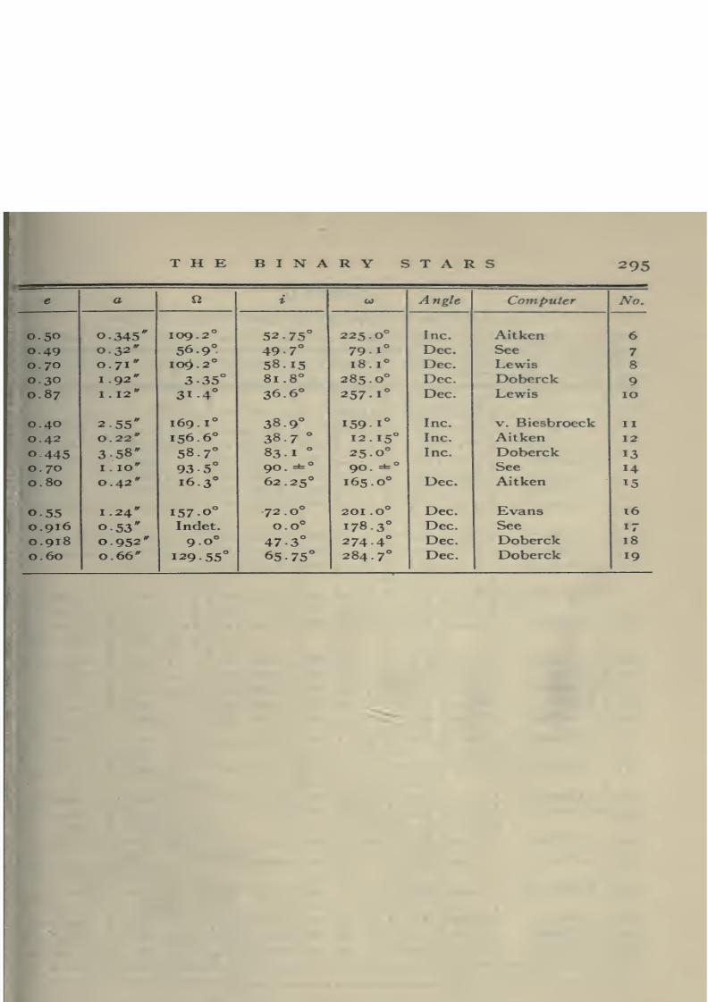
8/2/2019 The Binary Stars 1918
http://slidepdf.com/reader/full/the-binary-stars-1918 323/349
THE BINARY STARS 295
e a n i CO Angle Computer No.
0.50 0.345" 109.
2«
52.75'' 225.0° Inc. Aitken 60.49 0.32" 56.9° 49-7° 79.1° Dec. See 7
0.70 0.71" 109.2° 58.15 18.1° Dec. Lewis 8
0.30 1.92"' 3.35° 81.8° 285.0° Dec. Doberck 9
0.87 1. 12" 31.4^ 36.6° 257.1° Dec. Lewis 10
0.40 2.55" 169.1° 38.9° 159-1°
Inc. V. Biesbroeck II
0.42 0.22" 156.6° 38.7° 12.15° Inc. Aitken 12
0.445 3.58' 58.7° 83.1°
25.0° Inc. Doberck 13
0.70 1. 10" 93.5° 90.=^° 90. ±° See 14
0.80 . 42"
16.3° 62.25° 165.0° Dec. Aitken 15
0.55 1.24" 1570° 72.0° 201.0° Dec. Evans 16
0.916 0.53" Indet. 0.0° 178.3° Dec. See ^
0.918 0.952" 9.0'' 47.3° 274-4° Dec. Doberck 18
0.60 0.66" 129.55° 65 -75° 284.7° Dec. Doberck 19

8/2/2019 The Binary Stars 1918
http://slidepdf.com/reader/full/the-binary-stars-1918 324/349
TABLE IV
List of Orbits of Spectroscopic Binary Stars
A star preceding the figures in the column T indicates that the time is measured from a pt
ticular phase of the curve; from the epoch of light maximum, as in most of the Cepheid variablt
from the epoch of light minimum as in f Ceminorum, or from an epoch of maximum or of zero relati
radial velocity as in tt^ Orionis.
No. Star Mag. Sp. IQOO . 1900 . PT
2410000 4
I
2
3
4
5
a Androm.
Boss 82
13 Ceti
7r Androm.
7r Cass.
2.15
5.16
5-24
4-44
5.02
A
A2F
B3
A5
oh 3 2^
22.9™
30. I""
31-5"^
37.8-
+28° 32'
+43° 51'
- 4° 9'
+33° 10'
+46° 29'
96^67
3-956
2.082-
143.67-
1.964+
7882.40
8841.59c
7484. 48i
8564. I4z
9970.03;
_ 6
7
8
23 Cass,
f Androm.
V Androm.
5-39
4-30
4.42
B8
KB3
41. I"
42.0™
0M4-3™
+74° 18'
+23° 43'
+40° 32'
33-75
17.767+
4.283-
10577.41
10024.88]
9
10
a Urs. Min.
<f>Persei
Var.
Var.
F8
Bp
ih 22. 6""
37-4'"
+88° 46'
+50° 11'
13-968+
1 ii.9yr.
|i26.5
1 63.25
4890 . 04
4509.0
8290.42
*8326.58
II
12
13
14
15
o Triang.
oj Cass.
/3 Arietis
RZ Cass.
TT Arietis
3-58
5-03
2.72
Var.
5-30
F5
B8
A5
AB5
47.4"
48.2™
ii>49.i'«
2h39.
9^
2h^3
7m
+29° 6'
+68° 12'
+20° 19'
+69° 13'
+ 17° 3'
1-737"
69.92
107.0
I. 195+
3.854
10793.821
10426.02
7632.0
9449.73210370.259
i6
17
/3 Persei
o Persei
Var.
3-94
B8
Bi
3h lym
38.0"'
+40° 34'
+31° 58'
12.867+
1 1 .899yr.
4-419+
2.264
1901.855
8217.924
i8
19
20
$ Persei
X Tauri
n Persei
4-05
Var.
4.28
Oe5
B3
G
52.5'°
3^55-1™
4^ 7.6^
+35° 30'
+ 12° 12'
+48° 9'
6.951
f 3-953"
1 34-60
284.
8248.
308
7945.119
7831.30
10061.97
21 b Persei 4-57 A2 10.7"" +50° 3' 1.527+ 8956.166
22 1^4 Eridani 3.59 B9 14.1'° -34° 2' 5.010+ 7562.266
23
24
25
63 Tauri
02 Tauri
d Tauri
5.68
3-62
Var.
A2
A5
A2
17.7'"
22.9™
30.2°^
+ 16° 32'
+ 15° 39'
+ 9° 57'
8.425
140.70
3.571+
9819.0
8054.723
9734.992
1 The orbits listed in this Table are discussed in Chapter VIII.

8/2/2019 The Binary Stars 1918
http://slidepdf.com/reader/full/the-binary-stars-1918 325/349
TABLE II
List of Orbits of Spectroscopic Binary Stars
When two sets of elements are given, the lower figures for K and for a sin i relate to the secondcomponent if the two values for w differ by i8o°; if the lower value of P is an aliquot part of the
upper value, the lower line of figures relates to an assumed secondary oscillation; in other cases the
lower line relates to a third body definitely known or suspected in the system.
K Vo a sin i mi'sitiH
e
km. km. million km.Computer No.O
{m + wi)2
76.21° 0.525 30.75 -11-53 34 - 790 0.180O Baker I
233.2° 0.152 41.7 + 2.04 2.240 MissUdick 2
223.1° 0.062 34-35 + 10.5 0.981 0.0087 Fox 3
350.53° 0.573 47.66 + 8.83 77.200 0.876 Jordan 4
[45-1° 0.009 117.76 + 8.92 3.180+1 Harper 5
1225.1° 117.40 3.170+J
269.71° 0.405 16.32 — 4.06 7.020 0.0121 Young 6
182.22" 0.037 25-69 -29.83 6.272 Cannon 7
0.000 {75-63
[104.0
-23.91 4-454 1
6.125J
Jordan 8
80.0° 0.13 3-04 0.164 O.OOOOI Miss Hobe 9
293.0° 0.35 2.98 -14.8 166.800 . 0098
347-29° 0.428 26.90 + 3.20 42.298 0.189 Cannon 10
1257.14° 0.107 6.96
135-56° 0.121 12.10 -12.65 0.287 Harper II
49-97° 0.30 29.64 -24.82 27.190 0.164 Young 12
19-7° 0.88 32.6 - 0.6 22.880 0.042 Ludendorff 13
154-7° 0.052 69.30 -38.32 1. 137 0.0412 Jordan 14
78.27° 0.042 24.77 + 7.81 1.310 0.0061 Young 15
21.0° 0.060 41-3 + 3.40 1.630 0.021 Curtiss 16
0.000 9-4 + 4.1 89 . 000 . 060
0.000 fill. 92
|i6o.o
+ 18.46 6.801
9.717
0.754.
Jordan 17
99.18° 0.034 7-87 + 15-40 0.752 Cannon 18
77.5° 0.061 56.18 + 12.95 3-050 0.073 1Schlesinger 19
0.000 10.4 4.950 0.004 J
301.99° .062~ 20.50
+7-83 80 . 000 Cannon 20
151.75° 0.22 41.89 +23-09 0.838 Cannon 21
331.75° 152.5 3.048
124-33° 0.014 63-76 + 17-83 4.393 Paddock 22
[304-33° 64.85 4.468
190.7° 0.16 36.5 +36.4 4.170 0.041 Jantzen 23
54-16° 0.717 27.12 +42.59 37-471 Plaskett 24
0.000 72.68 +29.23 3-570 0.142 Daniel 25
TABLE II {Continued)

8/2/2019 The Binary Stars 1918
http://slidepdf.com/reader/full/the-binary-stars-1918 326/349
298 THE BINARY STARS
No. Star Mag. sp. Igoo . igoo.o PT
24ioooo-\-
26 SZ Tauri Var. F8 31.4™ + 18° 20' 3^.148+ IOOI6.I87
27 T Tauri 4-33 B5 36.2™ +22'' 46' 1-505" 7892.50c
28 9 Camelop. 4-38 B 44-1'" +66° 10' 7.996- 6480.35
29 7r4 Orionis 3.78 B3 45-9™ + 5° 26' 9-519"+ 8279.64
30 7r5 Orionis 3-87 B3 49.o«> + 2° 17' 3 - 700+ *792i.64
31 7 Camelop. 4-44 A2 4^49.3™ +53° 35' 3.885- 8281.176
32 14 Aurigae 5-14 A2 5h 8.8« +32° 35' 3-789" 10802.715
33 a Aurigae 0.21 G 9-3" +45° 54' 104.022 4899-5
34 ^ Orionis 0.34 B8p 9-7" - 8° 19' 21.90 7968 . 80
35 7; Orionis 3-44 Bi 19.4'° - 2"^ 29' 7.990- 5720.821
36 ^ Orionis 5-79 A 21. 6« + 3° 0' 2.526" 7916.36
37 X Aurigae 4.88 Bi 26.2" +32° 7' 655-16 10629.78
38 b Orionis Var. B 26.9™ - 0° 22' 5-732+ 9806.383
39 VV Orionis Var. B2 28.5™ - 1° 14'1
1-485+
[120.0
9836.021
9819.
40 I Orionis 2.87 Oes 30.5'" - 5° 59' 29.136 {7587-99117577-354
41 f Tauri 3.00 B3 31-7" +21° 5' 138.0 5769 -9
42 125 Tauri 5-00 B3 33-5" +25° 50' 27.864 10471.607
43 Boss 1399 5.00 B3 35-8- - 1° II' 27.160 7961.465
44 136 Tauri 4-54 A 47. o« -^2r 35' 5-969 9362.52
45 /3 Aurigae Var. Ap 52.2'« +44° 56' 3.960+ 7100.732
46 40 Aurigae 5-31 A 5^59-6™ +38° 29' 28.28 10468.197
47 V Orionis 4.40 B2 6h 1.9m +14° 47' 131.26 7975-16
48 Boss 1607 5-50 A 18. 0™ +56° 20' 9-944 9341-776
49 RT Aurigae Var. G 22.1'= +30° 34' 3-728+ *3-423
50 7 Gemin. 1-93 A 31-9™ +16° 29' 2175-0 101.6
51 f Gemin. Var. G 6** 58 .
2« +20° 43' 10.154 *i-3i3
52 29 Can. Maj. 4-90 Oe 7M4.5'" -24° 23' 4-393+ 7240.248
53 RCan. Maj. Var. F 14-9" -16° 12' 1-136+ 7966.576
54 <r Puppis 3-27 K5 26.1" -43° 6' 258.0 10419.0
55 ai Gemin. 2.85 A 28.2"" +32° 6' 2.928+ 6828.057
56 az Gemin. 1.99 A 9.219- 6746 385
57 (7 Gemin. 4.26 K 7»'37.o" +29° 7' 19.605 5824.019
58 c Volantis 4.46 B5 8^ 7-6™ -68° 19' 14.168+ 9453 562
59 *c Hydrae 3-48 F8 8»'4i.5" + 6° 47' 5588.0 5375-0
60 K Cancri 5-14 B8 ^h 2.
4« + 11° 4' 6.393 6486.897
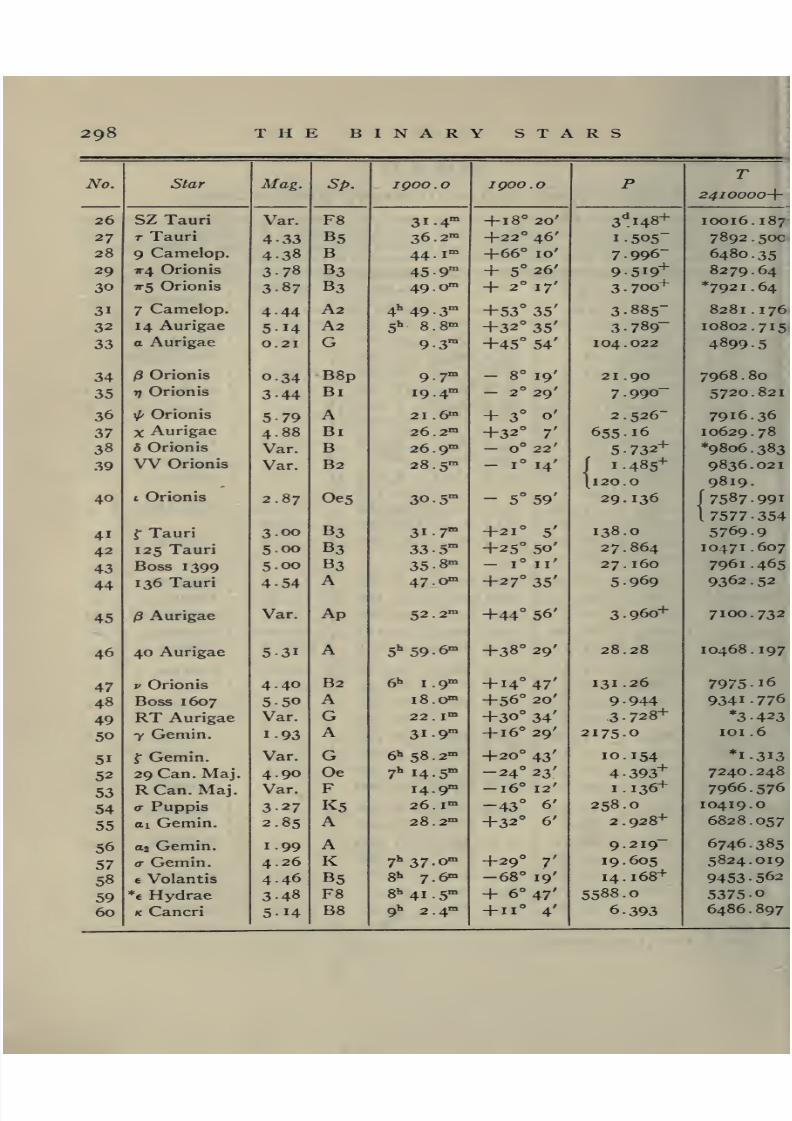
8/2/2019 The Binary Stars 1918
http://slidepdf.com/reader/full/the-binary-stars-1918 327/349
THE BINARY STARS 299
K Vo a sin i mi'sinHe
km. km. million km.Computer No.)
(m + w,)2
76.66° 0.24 10.94 - 3-15 0.460 0.0004 Hayncs 26242 .
88° 0.087 44-34 + 13.55 0.914 Parker 27
90.0° 0.30 9.0 - 2.25 Lee 28
152.27° 0.027 25 -93 +23.27 3.393 Baker 29
0.000 57-88 +24.20 2.945 Lee 30
217-14° 0.013 35-15 - 8.93 1.877 Harper 31
19.70° 0.033 21.56 -10.74 1. 123 Harper 32
117-3" 0.016"*" 25 76 +30.17 36.848 1 Reese 33
1297-3° 32.45 46.430 J
254-76° 0.296 3-77 +22.62 1. 109 O.OOOI Plaskett 34
42.3" 0.016 144-75 +35.5 15.901 2.51 Adams 35
184.71° 0.065 144.12 + 12.02 4-995 0.780 Plaskett 36
135-52° 0.171 20.53 - 0.15 182.300 0.56 Young 37
359-33° 0.098"*" 100.96 +20.15 7.926 0.605 Curtiss 38
0.000 132.37 +20.77 2.704 0.358 ] Daniel 39
40.0° 0.30 130 20.
460J
112.374° 0.742"
0.000
113-68
8.38
+21.53 30.560 1
3-358 J
Plaskett 40
9-8° 0.180 14-95 + 16.4 27.900 0.046 Adams 41
335-0° 0.55 25-5 + 14-8 8.160 Cannon 42
87.02° 0.765 93-04 +26.12 22.380 Harper 43
{191-44° 0.022 48.9 -17. 4.on ] Cannon 44
1 11-44° 71.0
0.000 108.96
1 1 1 . 04
-18. 5-934
6.047
Baker 45
178.40° 0.556 51-38 + 16.91 16.550 ]
20.140J
Young 46-1.60° 62.51
1.58° 0.599 34-09 +22.10 49.270 Harper 47
152.9° 0.081 67.19 -13.74 9.127 Harper 48
95-016° 0.368 17.96 +21.43 0.856+ Duncan 49
16.31° 0.298 6.12 -12.28 174-720 Harper 50
333-0° 0.22 13.2 + 6.8 1.798 0.0023 Campbell 51
37.64° 0.156 218.44 — 12.12 4-58 Harper 52
195-86° 0.138 28.64 -39-70 0.4430.0027 Jordan
53350.0° 0.2 18.0 +88.5 62
.570 Lunt 54
102.52° O.OI 31.76 - 0.98 1.279 Curtis 55
265.35° 0.503 13.56 + 6.20 1-485 Curtis 56
330.25° 0.022 34.21 +45 - 80 9.220 Harper 57
0.000 66.67 + 9-68 12.999 0.437 Sanford 58
90.0° 0.65 8.45 +36.78 493 000 Aitken 59
162.26° 0.149 67.8 +26.3 5.890 Ichinohe 60
TABLE II (Continued)

8/2/2019 The Binary Stars 1918
http://slidepdf.com/reader/full/the-binary-stars-1918 328/349
300 THE BINARY STARS
No.
6i
62
63
64
65
66
67
68
69
70
71
72
73
74
75
76
77
78
79
80
81
82
83
84
85
86
87
88
89
90
Star
a Carinae
Boss 2484
K Velorum
o Leonis
3oHUrs.Maj,
w Urs. Maj.
/3 Urs. Maj.
93 Leonis
Boss 3182
rj Virginis
d2 Virginis
e Urs. Maj.
a2 Can. Ven.
fi Urs. Maj.
a Virginis
Boss 351
V Centauri
h Centauri
7j Bootis
a Drac.
d Bootis
A Bootis
5 Librae
/3 Cor. Bor.
a Cor. Bor.
A 2 Serp.
/3 Scorpii
d Drac.
<r Scorpii
/3 Herculis
Mag.
356
570
2.63
376
4.92
4.84
2.44
4-54
512
4.00
524
1.68
2.90
2.40
1. 21
4.96
3-53
4.76
2.80
364
4.82
483Var.
3-72
Var.
5-37
2.90
4. II
3082.81
sp.
B3
A
B3
F5P
A
A
AF8
A5
A
Ap
ApAp
B2
F
B2
B5
GA
F5
G5
AFp
B8
Bi
F8
Bi
K
Igoo .
8.4™
10.8™
19.0™
9^ 35 .
8"*
ID** 16.9™
48.2™
10^55.8'°
I !•> 42 .
8'°
14.8'°
40.6™
49.6^
I2h 51.4m
13^ 19.9™
19.9"
30
43
47
13^4914^ I
13
is'* 23
30
40
15^59
i6»» o
15
25
Igoo .
-58° 33'
+47° 14'
-54° 35'
+ 10° 21'
+66° 4'
+43° 43'
+56° 55'
+20° 46'
+78° 10'
- 0° 7'
+ 8° 13'
+56° 30'
+38° 52'
+55° 27'
-10° 38'
+37° 42'
-41° II'
-31° 26'
+ 18° 54'
+64° 51'
+25° 34'
+35° 58'
- 8° 7'
+29° 27'
+27° 3'
- i°30'
-19° 32'
+58° 50'
-25° 21'
+21° 42'
6^744
[5.986
116.65
14.498
11.583+
15.840+
0.312+
71.70
1. 271
71.9
38.3
4.i5yrs.
55020.536+
4.014+
1.613-
2.625+
6.927
497.1
51.38
9 . 604+
211.95
2.327
[40.9
1490.8
17.36
38.95
6.828+
3.071-
0.247-
410.575

8/2/2019 The Binary Stars 1918
http://slidepdf.com/reader/full/the-binary-stars-1918 329/349
THE BINARY STARS 301
K Vo a sin i mi^sinHe
km km. million km.Computer No.O
(m + w,)2
115-84° 0.18 21.5 +23-3 1.960 Curtis 61
[355-2° 0.504 63.34 -I3-II 12.026 Harper 62
li75.2° 73.64 13.981
96.23° 0.19 46.5 +21.9 73.200 Curtis 63
< 0.02 [54 -0
163.
+27.07 10.775
12.571
0.238 1
0.378 J
Plummer 64
171.9° 0.381 34.07 — 0. 10 5.020 Schlesinger 65
11.95° 0.264 20.64 -18.45 4.336 Parker
Guthnick
66
315.4° 0.124 1.25 -10.93 2660 km. 0.000 and Prager 67
270.81° 0.008 26.54 + 0.17 26.170 Cannon 68
0.000 63.2 + 0.3 1. 104 Lee 69
185.0° 0.40 27.6 + 2.2 25.750 0.126 Harper 70
223.35° 0.072 40.99 - 8.89 21.530 Cannon 71
43-35° 80.0
55.8° 0.31 3.5 -12.9 69.360 . 0058 LudendorfT 72
110.0° 0.3 21.5 + i.o 1.500 Belopolsky 73103.96° 0.535 69.22 - 964 16.400 1 Hadley 74
283.96° 68.83 16.400J
328.0° O.IO 126. + 1.6 6.9301
Baker 75
148.0° 207.8 11.400J
201.5° 0.067 10.25 + 7.09 0.227" . 0002 Harper 76
0.000 20.63 + 9.05 0.745 0.0024 Wilson 77
147.23° 0.23 21.4 + 5.2 1.984 0.0065 Paddock 78
315.20° 0.236 8.69 - 0.2357-735
Harper79
19.07° 0.384 46.25 -17.03 30.173 Harper 80
273.0° 0.169 68.40 + 9.80 8.9041
Harper 81
1 93.0° 72.05 9.380 J
223.42° 0.54 18.02 +25.62 44 . 000 0.076 Young 82
29.2° 0.054 76.5 -45.0 2.450 Schlesinger 83
240.0° 0.4
0.000
3.10
2.4
-21.28 I . 600 1 Cannon 84
312.2° 0.38734-93 +
0.36 7.671 0.060 Jordan 85
208.46° 0.773 50.52 -11.63 17.170 0.133 Jordan 86
20.09° 0.270 125.66 — II.O 11.360 1 Daniel and S7
200 .09° 197.0 17.800
JSchlesinger
126.11° 0.014+ 23.47 - 8.36 0.990 0.004 Curtis 88
110.0° 0.05 39.0 + 2.0 0.129 0.0014 Selga 89
24.60° 0.550" 12.78 -25.52 60.280 0.052 Reese and
Plummer
90
TABLE II (Continued)

8/2/2019 The Binary Stars 1918
http://slidepdf.com/reader/full/the-binary-stars-1918 330/349
302 THE BINARY STARS
No. Star Mag. SP- Igoo . Igoo . PT
2410000+
91
92
€ Urs. Min.
e Herculis
4.40
392
G5
A
56.2'"
16^56.5""
+82° 12'
+31° 4'
39^482
4.024-
8005. 75
8086.253
93 u Herculis Var. B3 17^ 13.6™ +33° 12' 2.051+ 8125.80
94 Boss 4423 4.61 F 21.3™ - 5° 0' 26.274+ 8411.524
95 ^ Serp. 364 A5 31.9™ -15° 20' 2 . 292+ 9209.618
96
97
98
99
100
CO Drac.
X Sagittarii
Y Ophiuchi
W Sagittarii
M Sagittarii
4.87
Var.
Var.
Var.
4.01
F5
F8
GF5
B8p
37-5"
41.3'°
47-3'^
I7b58.6°>
i8»' 7.8^
+68° 48'
-27° 48'
- 6° 7'
-29" 35'
-21° 5'
5.280-
7.012-
17. 121"
7•
595~
180.2
7385-493
6723-05
*2.4i5
*6.20
4968.4
lOI
102
Y Sagittarii
108 Herculis
Var.
5-54
GA
15-5™
17.1'"
-18° 54'
+29° 48'
5-773"^
5-5i5~
*4-46
9551-742
103
104
105
X Drac.
RX Herculis
f 1 Lyrae
369Var.
4.29
F8
AF
22.9'"
26.0°'
41.3'"
+72^41'
+ 12° 32'
+37° 30'
281.8
I.
779~
4.300-
4864.3
9658.588
8109.722
106 /3 Lyrae Var. B2p 46.4- +33° 15' 12.919+ *9.867
107 50 Drac. 5-37 A 49.6- +75° 19' 4.120 10293-93
108
109
no61 Lyrae
113 Herculis
5-51
4-56
5.10
B3
G5
B8
50.2'°
18'^ 50.5"
+36^51'
+22° 32'
+ 10° 55'
88.112
245 -3
1.302+
9220.727
9805 .
*8i57-502
III
112
113
114
115
18 Aquilae
U Sagittae
V Sagittarii
2 Sagittae
RR Lyrae
a Aquilae
Var.
4-58
6.03
Var.
517
AB8p
A
F
B8
14.4'°
i6.o°»
19.8™
22.3™
34-3"^
+ 19° 26'
-16° 8'
+ 16° 45'
+42° 36'
+ 5° 10'
3-381-
137 -939
7-390
0.567-
1.950+
8428.183
9648.72
10943-233
0.508
10054-331
116
117
118
SU Cygni
77 Aquilae
6 Aquilae
Var.
Var.
3-37
F5
GA
40.8°»
19^ 47.4m
20^^ 6.1='
+29° I'
+ 0° 45'
- 1° 7'
3-844
7.176
17.124+
*2.5
6.210
8261.914
119
120
/S Capricorni
a Pavonis
3 25
2.12
Gp
B3
15 ^"^
17.7'"
-15° 6'
-57° 3'
1375-3
11-753
6035.0
6379.90

8/2/2019 The Binary Stars 1918
http://slidepdf.com/reader/full/the-binary-stars-1918 331/349
THE BINARY STARS 303
K Vo a sin i mi^sinHComputer No,) &
km. km. million kn. (m + m,)2
359 46° 0.011+ 31-954 -11.398 17-346 Plaskett 91
180.0° 0.023 70.39 -24.03 3-890 Baker 92
0.0° 112. 6.200
66.15° 0.053 99-50 -21.16 2.800 Baker 93
246.15° 253-0 7.120
14.48° 0.491+ 47-49 + 0.44 14-950 Parker 94
194.48° 50.67
0.000 19-35 -42-77 0.610 Young 95
333 76° O.OII" 36.26 -13.68 2.632 Turner 96
93-65° 0.40 15-2 -13-50 1-334 Moore 97
201.7° 0.163 7.70 - 5-10 1.790 Miss Udick 98
70.0° 0.320 19-5 -28.6 1.930 0.005 Curtiss 99
74-7° 0.441 645 - 7-0 143.500 Ichinohe 100
32.0° 0.16 19.0 + 4-0 1-485 Duncan 101
0.000I70.1
.101.7
—20.2 5-320 1
7.710 J
Daniel and
Jenkins
102
119.0° 0.423 17-95 +32.38 62 . 020 Wright 103
0.000 106.0 -18.5 2.590 Shapley 104
0.000 51-24 -2597 3-030 Jordan 105
0.15° 0.018 184.40 -20.95 32.7501
Curtiss 106
180.15° 75-0 13-300J
(151-0° 0.024 75-77 — 10. 4.291I
Harper 107
1331-0° 83.26 4.716J
204.55° 0.28 33-68 -25.85 39220
0.309Jordan 108
169-5° 0.12 16.0 -23.2 53.580 0.102 Wilson 109
0.000 27-59 -18.65 0.494 0.0028 Jordan no
44-14° 0.035 66.45 -19-13 3.090 Miss Fowler III
28.6° 0.087 48.15 + 12. 91 .010 1.582 Wilson 112
(332.6° 0.05 52.95 + 11. 5-370 1 Young "3
1152.6° 73-8 7-490 J
96.85° 0.271 22.2 -68.7 0.166+ 0.00057 Kiess 114
0.000(163-52I199.0
-5-0 4-380
5-340 J
Jordan 115
(345-8°) 0.2I=t 25-=^ -33-4=*= 1-350=^ 0.0058^ Maddrill 116
68.91° 0.489 20.59 — 14.16 1-773 0.0043 Wright 117
I14-9° 0.681 46.0 -30.5 7 930 Baker 118
li94-9° 63.0 10.860
124.0° 0.44 22.2 -18.8 377.000 Merrill 119
224.80° O.OI 7-25 + 2.0 1. 170 Curtis 120
TABLE II {Continued)

8/2/2019 The Binary Stars 1918
http://slidepdf.com/reader/full/the-binary-stars-1918 332/349
304 THE BINARY STARS
No. Star Afag. sp. igoo . Igoo . PT
2410000+
121
122
T Vulpec.
57 Cygni
Var.
4.68
F
B3
47.2-
20^ 49 .
7™
+27° 52'
+44° 0'
4^436-
2.855
*3.678
8554-770
123
124
125
/3 Cephei
1 Pegasi
2 Lacertae
Var.
3964.66
Bi
F5
B5
21'' 27.4"'
22^^ 2.
4™
16.9™
+70° 7'
+24° 51'
+46° 2'
0.190+
10.213+
2.616+
9638.812
4820.
966
8193.30
126
127
128
129
130
5 Cephei
12 Lacertae
77 Pegasi
9 Androm.
I H Cass.
Var.
5-18
3.10
5 90
4.89
GB2
GA2
B3
25.4™
37.0-
22^38.3™23h
137m
25-4"
+57° 54'
+39° 43'
+29° 42'
+41° 13'
+58° 0'
5.366+
0.193+
818.0
3.219+
6.067
7888.428
10761.149
5288.7
11059-921
8223.
762
131
132
X Androm.
Boss 6142
4.00
6.05
KBp
32.7m
23^50.5-
+45° 55'
+56° 53'
20.546
13-435
6683.46
10800.634
I
2
3
4
5
a Persei
a Orionis
P Can. Maj.
p Leonis
a Scorpii
1.90
0.92
1.99
3-85
1.22
F5
MaBi
Bp
Map
3h17 2^
5^49-8-
6i»i8.3°>
10** 27.5'"
i6h 23.3m
+49° 30'
+ 7° 23'
-17° 54'
+ 9° 49'
-26° 13'
4.094-
6 . yrs.
0.25
12.28
5 . 8oyrs.
7955-14
6693.
8749.603
6673.582

8/2/2019 The Binary Stars 1918
http://slidepdf.com/reader/full/the-binary-stars-1918 333/349
THE BINARY STARS 305
f Oi
K Vo a sin i mx^sinHe
km. km. million km.Computer No.
(W+Wi)2
104.03° 0.440 17.63 - 1.39 0.966 0.0018 Beal 121
145.0° 0.137 no. -16.2 4.200 1 Baker 122
1225.0° 118. 4.620J
2.63° 0.040 15.798 -14.13 0.041" Crump 123
251.81° 0.0085 47.99 - 4.12 6.740 Curtis 124
ji8o.o° 0.015 80.3 - 9.0 2.890 1 Baker 125
ij 0.0° 98.8 3.550 J
85.385° 0.484 19.675 -16.83 1. 271 0.0028 Moore 126
0.000 16.92 -13.75 0.045 O.OOOI Young 127
5.605° 0.155 14.20 + 4-31 157.800 Crawford 128
40.57° . 0365 73.56 - 4.87 3.240 0.133 Young 129
i
3.35° 0.224 59.06 -14.78 4.920 Baker 130
301.0° 0.086 7.07 + 7.43 1.990 Burns 131
{339.56° 0.105 115. -26.7 21.200 1 Young 132
1159.56° 167. 30.700J
221.0° 0.47 0.93 - 3-43 0.046 0.0000 Hnatek I
255.0° 0.24 2.45 4-21.3 70.000 0.003 Bottlinger 2
o.i=fc 9.8± +33.7^ 0.034- Albrecht 3
180. =t° 0.5=^ 10. =fc +41.1 Schlesinger 4
289.0° 0.20 2.12 - 3 09 Halm 5

8/2/2019 The Binary Stars 1918
http://slidepdf.com/reader/full/the-binary-stars-1918 334/349

8/2/2019 The Binary Stars 1918
http://slidepdf.com/reader/full/the-binary-stars-1918 335/349
STAR LISTi
A 88 84, 232
A 1079 224
A 1813 224
A 2286 224
Aldebaran 2
Algol 28,
. . 29, 167, 168, 247-250
7 Andromedae . . 253, 278
X Andromedae .... 246
4 Andromedae .... 205
a Aquilae 205
7] Aquilae 221
6 Aquilae 205, 206, 246, 275
4 Aquarii 6Arcturus 2
7 Arietis i
a Aurigae 205
/3 Aurigae . 29, 205, 244-246
X Aurigae .... 198, 243
RT Aurigae 221
40 Aurigae 205
d Bootis 205
e Bootis 6, 264
^ Bootis 216, 264
Boss 2184 205
Boss 4423 205
Boss 6142 205
9 Camelopardalis . . . 243
f Cancri ... 6, 102, 216,
. . . 223, 234, 253, 264
^ Canis Majoris .... 193
R Canis Majoris
29 Canis Majoris
f Capricorni .
a Carinae . .
190
208
232
114
rj Cassiopeiae 208,
209, 216, 264
7r Cassiopeiae 205
Castor ... I, 2, 4, 9, 32,
.... 65, 224, 240, 244
Celaeno 46a Centauri . . . I, 2, 4, 36,
114, 122, 124, 127, 209,
. 216, 217, 226-230, 237
/3 Cephei 195, 220
8 Cephei 221
13 Ceti 223
82 Ceti 54
42 Comae Berenices . 95, 232
7] Coronae Borealis . . 209
<T Coronae Borealis . . 193
a Crucis i, 36
SU Cygni 221, 223
57 Cygni 205
61 Cygni . I, 104, 226, 253
W Delphini .... 181, 188
50 Draconis 205
Electra 46
d Equulei . . 194, 209, 232
e Equulei 54> 99
7 Eridani . . . 114, 115, 205
40 02Eridani
209, 235, 236, 237, 265
7 Geminorum 198
K Geminorum 2
f Geminorum . . . 163, 221
(T Geminorum 2
8 Herculis 6
e Herculis .... 205, 246
^ Herculis 102, 103, 209, 216
1 No reference is made in tiiis list to the Tables of Orbits on pages 290-305.

8/2/2019 The Binary Stars 1918
http://slidepdf.com/reader/full/the-binary-stars-1918 336/349
308 THE B I N A
fjL Herculis
209, 235, 236, 264, 265
u Herculis .... 205, 206
108 Herculis 205
Hu 66 224
Hu 91 224
a Hydrae loi
€ Hydrae loi, 198, 209, 210,
... 216, 234, 253, 264
Krueger 60 . . . 209, 216,
230, 231, 275
2 Lacertae 205
7 Leonis 61
o Leonis 205
p Leonis 193
/3 Lyrae 167, 168,
. 201, 205, 206, 208, 250
RR Lyrae . . . 195, 220, 221
r Ophiuchi 6Y Ophiuchi 221
70 Ophiuchi
102, 209, 216, 250, 264
a Orionis 193
j8 Orionis loi
5 Orionis 241, 242
77 Orionis 205
Orionis i, 4, 284^ Orionis 205
02:351 224
S 476 224
K Pegasi . . . 223, 232, 250
85 Pegasi . 209, 216, 232, 233
a Persei 193
b Persei 205
o Persei 205
R Y STARS
Persei 193, 250
Pleiades 45» 46
Polaris
237-240
59, loi,
228, 247
237
205
xiii
221
221
221
. 207, 221, 223,
Procyon ..... . . 209, 216,
Proxima Centauri
2 Sagittae
V Sagittarii
W Sagittarii
X Sagittarii
Y Sagittarii
a Scorpii
/3 Scorpii
Sirius
216,
193
205
2, 59, loi, 209,
. 228, 229, 233,
..... 244, 247, 264
S 2026 94
S 3062 264X Tauri 205
SZ Tauri 221
80 Tauri 49, 50
136 Tauri 205
€ Ursae Majoris .... 198
^ Ursae Majoris i,
. . . 6, 7, 27-29, 63, 205
^ Ursae Majoris 209, 216, 264W Ursae Majoris .... 190
03 Ursae Majoris .... 205
30H Ursae Majoris .... 246
K Velorum .... 141, 146
a Virginis 29, loi, 205, 244
7 Virginis .... i, 4, 216
d2 Virginis 205
T Vulpeculae 221

8/2/2019 The Binary Stars 1918
http://slidepdf.com/reader/full/the-binary-stars-1918 337/349
INDEX OF NAMESI
Adams 230, 231, 235, 264, 265
Airy 18
Albrecht 220
Alter 104, 105
Andr^ 106
Argelander 247
Arrhenius 278
Astrand 74
Auwers loi, 229
Baker . . . 191, 224, 244-246
Barnard
vii, 24, 46, 47, 59, 230, 231
Barr 201
Bell 264
Belopolsky . . . 116, 240, 248
Bessel
13, 19, 100, loi, 228, 229, 247
Bickerton 278
Bishop 18
Bode 3, 4
Bohlin 219
Bond I, 63, 229
Boothroyd 23
Bosler 61
Boss 215, 216, 233
Bowyer 233
Bradley i, 2, 14
Burnham 17, 19-24, 26, 33-35,
38,52,57,59,73, 193,219,229,
230, 232, 253
Burns 31, 246
Campbell , . . vii, 30, 31, 44,
72, 116, 117, 127, 132, 195,
. . . 198, 204, 220, 222, 224,
• . . 230, 237-239, 250, 251,
281-283, 287, 288
* No reference is made in this list to the
Cannon, Miss A. J
vii 112, 263, 264
Chandler 247
Clark, A. . . . 18, 22, 24, 235
Clark, A. G loi, 229
Clerke, Miss A. M 250
Cogshall 23
Comstock 45, 67, 94,
. . . 102, 103, 233, 253, 262
Cornu 123, 131
Crossley 34
Curtis . . . vii, 30, 31, 143,
. . . 146, 149, 165, 240, 241
Curtiss 128, 133,
161, 165, 166, 222, 223, 225, 248
Darwin . . 190, 282, 283, 289
Dawes ... 18, 52, 56, 62, 67
Dembowski . 18, 19, 22, 52, 67
Ditscheiner 126
Doberck I93-I95,
218, 227, 240
Doolittle 34, 35, 230
Doppler 107
Duncan 225
Dunlop 36
Eddington 210
Elkin 46, 227
Encke 66, 67
Englemann 19
Espin 23, 35, 253
Everett, Miss A 218
Feuille 2
Fizeau 108
Flammarion 33
Fontenay i
Fox 34, 63, 64
Tables of Orbits on pages 290-305-

8/2/2019 The Binary Stars 1918
http://slidepdf.com/reader/full/the-binary-stars-1918 338/349
310 THE BINARY STARS
Frost 127, 132, 243
Furner 233
Furness, Miss C 191
Galileo 4
Gill 40, 227
Glasenapp 67, 74, 78-80, 84-86
Gledhill I9» 34
Goodericke 28, 247
Gould 64
Guthnick 195
Hagen 191
Hall 22, 33, 106
Halley 2
Hargrave 37
Harper 162, 246
Harting 168
Hartmann 123, 129, I3i-I33» 242
Henroteau . 160, 166, 250, 251
Henry 64Herschel, J. 9, 10, 15, 21, 26, 33,
35-37, 40, 66, 67, 71, 226, 253
Herschel, W. . . . xiii, 3-13,
IS, 21, 26, 33, 35, 40, 65, 223,
236, 253, 281
Hertzsprung . . . .64, 212-214
220, 225, 239, 272
Holden 24, 34Hooke I
Hough .... 23, 33, 34, 253
Howard 67, 106
Howe 24
Huggins 116
Humboldt 228
Hussey .... 17, 25, 26, 34,
38, 56, 57, 72, 73, 209, 223, 253
Huyghens i
Innes . 36-39, 53, 61, 210, 237
Jacobi 282
Jeans 280, 286, 289
Jonckheere .... 24, 35, 253
Jordan 242
Kant 281
Kapteyn .... 233, 244, 249
Kayser 132
Keeler 132
Kelvin 278
Kepler 81
King .... 154-157, 162, 165
Kirchoff iii
Klinkerfues 67, 105
Knott 19
Kowalsky67, 74,
78-80,84-86,95
Kustner 24, 34
Lacaille 226
Lambert 2
Laplace 281, 284
Laplau-Janssen 225
Lau 64
Laves 160, 165
Lee 243Lehmann-Filhes . 31, 142, 143,
146, 148, 150, 160, 165, 209
Leuschner 65, 106
Lewis ... 3, 14, 16, 20, 34,
56, 57, 60, 104, 193, 218, 263
Lohse 227, 229
Loud 225
Ludendorff
195, 201, 208, 222, 224, 225
Lunt 193
Maclaurin 282
Madler ........ 19, 66
Maury, Miss A. ... 29, 112
Mayer, C 3, 4
Mayer, T 223
Michell 2, 8
Moore vii, 31, 107
Moulton
vii, 96, 278-280, 285, 286, 289
Newall 132
Newton 65
Nijland 165

8/2/2019 The Binary Stars 1918
http://slidepdf.com/reader/full/the-binary-stars-1918 339/349
THE B I N A
Opik 217
Paddock 31, 162, 163, 164, 166
Passement 11
Peters loi, 229
Pickering vii, i, 27, 64, 112, 168,
239, 248, 253, 262, 263, 266
Plummer 164, 165
Poincare 282
Pollock 37
Poor 219
Pound I, 2
Ptolemy xiii
Rambaut . . 31, 106, 148, 164
Riccioli I
Richaud i
Roberts 168, 225, 227
Rowland .... 123, 127, 128
Russell, H. C 37
Russell, H. N vii, 67,
80, 99, 100, 148, 158-160, 164,
. . . 165, 168-177, 181, 184,
. . . 187, 190, 191, 212, 218,
. . . 220, 225, 231, 272, 283,
285, 286, 288, 289
Safford 229
Salet 61
Savary 66, 67
Schaeberle loi
Scheiner 116, 132
Schiaparelli .... 19, 33, 59
Schlesinger ... 62, 63, 104,
105, 138, 160, 161, 163, 166,
. . . 195, 201, 204, 206, 224,
231, 244, 245, 248
Schonfeld247
Schorr 106
Schuster 55
Schwarzschild .... 67, 106,
. . . 139, 149, 150-152, 165
Secchi 19, 112
R Y STARS 311
See . . 23, 67, 73, 91, 106, 194,
209, 218, 227, 283-285, 289
Seeliger 67, 102,
. . . 106, 234, 255, 258, 269
Sellors 37
Shapley 168, 188-191,
. . . 216, 217, 225, 249, 272
Smythe 18
South 9-11, 21
Stebbins. . . 190, 241, 247-249
Steele, Miss H. B 211
Stone 24
Stoney 276-279
Struve, F. G. W. . . 11-18,21,
• • • 26, 33, 34, 36, 67, 99,
232, 235, 253, 263
Struve, H 62
Struve, 17, 19, 21,
... 25, 26, 34, 50, 232, 253
Thiele, H 64
Thiele, T. N. . . 67, 105, 106
Tisserand 168
Triimpler 46
Turner 218
Van BiesbroeckJ215
Villarceau 66
Vogel . . 28, 29, 116, 132, 248
Vodte 62
Webb 22, 23
Weersma .... 233, 244, 249
Wendell 182
Wilsing 148, 164, 165
Wilson, J. M 19, 34
Wilson, R. E 31
Wright 31,
... 117, 119, 132, 209, 227
Young vii, 137, 138, 158,242,243
Zurhellen
. 139, 149-151, I53» 163-165
Zwiers . . 67, 74, 80-83, 89, 95

8/2/2019 The Binary Stars 1918
http://slidepdf.com/reader/full/the-binary-stars-1918 340/349
GENERAL INDEX
Angstrom unit defined . . : 1 1
Binary stars
Capture theory of origin of 276
Cepheid variables regarded as 219, 239
Definitions of xiii
Densities of 216
Distribution of, by spectral class 265
Distribution of, in space 272
Fission theory of the origin of 282
Masses of 202-216
Multiple systems 223, 234, 235, 237
Number of known orbits of 192
Relations between period and eccentricity in 194Relations between period and spectral class in 198
Separate nuclei theory of the origin of 284
Statistical study of, in northern hemisphere 252-273
Summary of the facts of observation of 274
Systems of special interest 226
Tables of the known orbits of 192, 290, 296
See also. Double Stars, Eclipsing Binary Stars, Spectroscopic
Binary Stars, Visual Binary Stars.
Cepheid variables regarded as binary systems 219,239
Color contrast in double stars 16, 263
Diaphragms used in measuring double stars 58
Dispersion curves. Construction and use of 123, 126
Doppler-Fizeau principle 108
Double stars
Accidental errors in measures of 59
Burnham's career as observer of 21
Color contrast in 16, 263
Conventions for measures and records of I5» 40
Diaphragms used in measuring 58
Distribution of, by angular distance and magnitude .... 260
Distribution of, by galactic latitude and angular distance . . 259

8/2/2019 The Binary Stars 1918
http://slidepdf.com/reader/full/the-binary-stars-1918 341/349
THE BINARY STARS 313
Distribution of, by magnitude and galactic latitude .... 256
Distribution of, by magnitude and spectral class 270
Distribution of, by spectral class and angular distance . . . 272
Distribution of, by spectral class and galactic latitude . . . 268
Distribution of, in right ascension and declination 255
Earliest discoveries of i
Early speculations on the binary character of 2
First collection of3
General catalogues of 34. 35
Herschel's discoveries and theories 4
Herschel (J.) and South's work on 10
Lick Observatory survey for 24, 252
Magnitude estimates of 52
Method of measuring 48
Modern period of work on 21
Observing program for 53
Percentage of , among stars to 9 . o magnitude 255
Percentage of close pairs in certain catalogues of 26
Photographic measures of 63
Precautions to be observed in measuring 51
Recent discoveries and measures of 23, 33
Southern Hemisphere work on 36
Struve (F. G. W.), and the Mensurae Micrometricae .... 11
Struve (Otto), and the Pulkowa Catalogue 17
Systematic errors of measures of 60, 62, 69
Use of total reflecting prism in measuring 61
Working definition of 252
See also. Binary Stars, Visual Binary Stars.
Driving clock. The first II
Eclipsing binary stars
Definition of 167
Definitions of the orbit elements of 169
Example of orbit computation of 181
Formulae for density of 187
Number of 168
Russell's method of computing the orbits of 168-188
Shapley's discussion of the known orbits of 188
Evolution of a star 281
Eye-pieces, Method of finding the magnifying power of ... . 58
Gravitation, Universality of the law of 65

8/2/2019 The Binary Stars 1918
http://slidepdf.com/reader/full/the-binary-stars-1918 342/349
314 THE BINARY STARS
Kirchoff's law iii
Lick Observatory double star survey 24, 252
Magnifying power of eye-pieces 58
Magnitude estimates of double stars 52
Micrometer
Description of 40
Methods of determining the screw-value of 42, 44
Methods of determining the zero-point, or "parallel" .... 42
Of the 40-inch Yerkes telescope, Barnard's measures of the
screw-value of 46
Multiple stars 223, 234New Draper Catalogue of Stellar Spectra 263
Orbit of A 88 84
Orbit of W Delphini 181,188
Orbit of € Equulei 99
Orbit of K Velorum 146
Orbits of systems of special interest 226
Parallel, Method of determining 42
Photographic measures of double stars 63
Proper motions of stars, Halley's discovery of the 2
Radial velocity of a star
Chapter on the, by J. H. Moore 107-133
Components of the observed 127
Correctness of measures of the, how tested 131
Early determinations of the 116
Modern precision of measurement of the 116
Precautions to be taken in observing the 118
See also: Spectrograms, Spectrograph^ Spectroscope.
RectiHnear motion 103
Resolving power of a spectroscope no
Resolving power of a telescope 55
Spectrogram of 0.2 Centauri, Measurement and reduction of . . 122
SpectrogramsConstruction and use of dispersion curves in reducing . 123, 126
Cornu-Hartmann formulae for 123
Measurement of 122
Principles governing choice of reduction methods for . ... 131
Spectro-comparator method of reduction of 129
Velocity-standard method of reduction of 128

8/2/2019 The Binary Stars 1918
http://slidepdf.com/reader/full/the-binary-stars-1918 343/349
THE BINARY STARS 315
Spectrograph
Description of the Mills, of the Lick Observatory 117
Loss of light in a stellar
120Relative advantages of refractor and reflector when used in
connection with a stellar . 120
Spectroscope
Essential parts of a 109
Resolving power of a no
Spectroscopic Binary Stars
American observatories, and work on 30, 32
Conditions of the problem of computing orbits of 134
Definitions of the orbit elements of 72, 137
Differential formulae for correcting orbits of 160
Discoveries of 30
Distribution of, by spectral class and galactic latitude . . . 269
Distribution of the longitude of periastron in orbits of. . .
201
Earliest discoveries of i, 27
Equation for radial velocity of 135
Example to illustrate Lehmann-Filhes's orbit method for , 146
First solution of the problem of determining orbits of ... 31
King's orbit method for 154
Lehmann-Filhes's orbit method for 142
Lengthening of period in 246
Masses of 205
Number of known 30
Number of known orbits of 31, 192
Orbits of, with small eccentricity 164
Period of revolution of, how determined 137
References to orbit methods for 148, 160
Relative masses in 205
Russell's short orbit method for 158
Schwarzschild's orbit method for 149
Secondary oscillations in orbits of 162, 245
Stationary H and K lines in 242
Table of orbits of I93. 296
Velocity curve for I39» 141
Zurhellen's orbit methods for • 150
See also Binary Stars

8/2/2019 The Binary Stars 1918
http://slidepdf.com/reader/full/the-binary-stars-1918 344/349
3l6 THE BINARY STARS
Spectroscopy, Fundamental principles of loi
Spectrum, Definition of 109
Star of smallest known mass 231
Stellar spectra
Classifications of 112
Causes of line-displacements in 115
Examples of 114
Systematic errors in binary star measures 60-63, 69
Telescope, Resolving power of a 55
Tables of the orbits of spectroscopic binary stars 296
Tables of the orbits of visual binary stars 290
Total reflecting prism, use of in double star measures 61
Variable proper motion loi, 228
Visual binary stars
Apparent ellipses of 67
Construction of the apparent ellipse for, from the elements . 90
Corrections to be applied to the measures of 68Definitions of the orbit elements of 72
Early methods of determining the orbits of 66
Examples of orbit computation 84, 99
Formulae for differential corrections to orbits of ... 92, 94, 99
Formulae for ephermerides for 73
Formulae for orbits of, when i = 90° 95
General equation for the apparent ellipse 70
Glasenapp's modification of Kowalsky's orbit method for. .
78
Interpolating curves for 71
Kowalsky's orbit method for 74
Masses of 209
Methods of determining relative masses in ........ 214
Minimum hypothetical parallax of 213
Number of known orbits 192
Parallax of, from spectrographic measures 209
Parallelism of orbit planes of 218
Relations between period, semi-major axis, and parallax of . 211
Russell's statistical studies of 212
Table of orbits of 192, 290
With invisible component, or components 100
Zwiers's orbit method for 80

8/2/2019 The Binary Stars 1918
http://slidepdf.com/reader/full/the-binary-stars-1918 345/349

8/2/2019 The Binary Stars 1918
http://slidepdf.com/reader/full/the-binary-stars-1918 346/349

8/2/2019 The Binary Stars 1918
http://slidepdf.com/reader/full/the-binary-stars-1918 347/349

8/2/2019 The Binary Stars 1918
http://slidepdf.com/reader/full/the-binary-stars-1918 348/349

8/2/2019 The Binary Stars 1918
http://slidepdf.com/reader/full/the-binary-stars-1918 349/349
86P 16 wn
QB Aitken, Plobert Grant
821 The binary starsA3
Physical &
Appfied Sci.
PLEASE DO NOT REMOVE
CARDS OR SLIPS FROM THIS POCKET
UNIVERSITY OF TORONTO LIBRARY