THE BETA ODD LOG-LOGISTICGENERALIZED FAMILY OF DISTRIBUTIONS

Gauss M. Cordeiro∗, Morad Alizadeh†, M. H. Tahir‡,§, M. Mansoor¶, MarceloBourguignon‖ and G. G. Hamedani∗∗

AbstractWe introduce a new family of continuous models called the beta oddlog-logistic generalized family of distributions. We study some of itsmathematical properties. Its density function can be symmetrical,left-skewed, right-skewed, reversed-J, unimodal and bimodal shaped,and has constant, increasing, decreasing, upside-down bathtub andJ-shaped hazard rates. Five special models are discussed. We ob-tain explicit expressions for the moments, quantile function, momentgenerating function, mean deviations, order statistics, Renyi entropyand Shannon entropy. We discuss simulation issues, estimation by themethod of maximum likelihood, and the method of minimum spacingdistance estimator. We illustrate the importance of the family by meansof two applications to real data sets.

Keywords: Beta-G family, characterizations, exponential distribution, gener-alized family, log-logistic distribution, maximum likelihood, method of minimumspacing distance.

2000 AMS Classification: 60E05; 62E10; 62N05.

1. Introduction

There has been an increased interest in defining new generators or generalized(G) classes of univariate continuous distributions by adding shape parameter(s)to a baseline model. The extended distributions have attracted several statisti-cians to develop new models because the computational and analytical facilitiesavailable in programming softwares like R, Maple and Mathematica can easilytackle the problems involved in computing special functions in these extendedmodels. Several mathematical properties of the extended distributions may be

∗Department of Statistics, Federal University of Pernambuco, 50740-540, Recife, PE, Brazil,Email: gauss@de.ufpe.br, gausscordeiro@gmail.com

†Department of Statistics, Persian Gulf University of Bushehr, Bushehr, P. O. Box 751691-3798, Iran, Email: moradalizadeh78@gmail.com

‡Department of Statistics, The Islamia University of Bahawalpur, Bahawalpur 63100, Pak-istan, Email: mtahir.stat@gmail.com, mht@iub.edu.pk

§Corresponding Author.¶Department of Statistics, The Islamia University of Bahawalpur, Bahawalpur 63100, Pak-

istan, Email: mansoor.abbasi143@gmail.com‖Department of Statistics, Federal University of Pernambuco, 50740-540, Recife, PE, Brazil,

Email: m.p.bourguignon@gmail.com∗∗Department of Mathematics, Statistics and Computer Science, Marquette University, WI

53201-1881, Milwaukee, USA, Email: g.hamedani@mu.edu

2

easily explored using mixture forms of the exponentiated-G (“exp-G” for short)distributions. The addition of parameter(s) has been proved useful in exploringskewness and tail properties, and also for improving the goodness-of-fit of the gen-erated family. The well-known generators are the following: beta-G by Eugene etal. [15] and Jones [29], Kumaraswamy-G (Kw-G) by Cordeiro and de Castro [10],McDonald-G (Mc-G) by Alexander et al. [1], gamma-G type 1 by Zografos andBalakrishnan [53] and Amini et al. [6], gamma-G type 2 by Ristic and Balakrish-nan [44], odd-gamma-G type 3 by Torabi and Montazari [50], logistic-G by Torabiand Montazari [51], odd exponentiated generalized (odd exp-G) by Cordeiro et al.[12], transformed-transformer (T-X) (Weibull-X and gamma-X) by Alzaatreh etal. [3], exponentiated T-X by Alzaghal et al. [5], odd Weibull-G by Bourguignonet al. [7], exponentiated half-logistic by Cordeiro et al. [13], logistic-X by Tahir etal. [47], T-XY-quantile based approach by Aljarrah et al. [2] and T-RY byAlzaatreh et al. [4].

This paper is organized as follows. In Section 2, we define the beta odd log-logistic generalized (BOLL-G) family. Some of its special cases are presented inSection 3. In Section 4, we derive some of its mathematical properties such asthe asymptotics, shapes of the density and hazard rate functions, mixture rep-resentation for the density, quantile function (qf), moments, moment generatingfunction (mgf), mean deviations, explicit expressions for the Renyi and Shannonentropies and order statistics. Section 5 deals with some characterizations of thenew family. Estimation of the model parameters and simulation using maximumlikelihood and the method of minimum spacing distance are discussed in Section6. In Section 7, we illustrate the importance of the new family by means of twoapplications to real data. The paper is concluded in Section 8.

2. The odd log-logistic and beta odd log-logistic families

The log-logistic (LL) distribution is widely used in practice and it is an alter-native to the log-normal model since it presents a hazard rate function (hrf) thatincreases, reaches a peak after some finite period and then declines gradually. Itsproperties make the distribution an attractive alternative to the log-normal andWeibull models in the analysis of survival data. If T has a logistic distribution,then Z = eT has the LL distribution. Unlike the more commonly used Weibulldistribution, the LL distribution has a non-monotonic hrf which makes it suitablefor modeling cancer survival data.

The odd log-logistic (OLL) family of distributions was originally developed byGleaton and Lynch [18, 19]; they called this family the generalized log-logistic(GLL) family. They showed that:– the set of GLL transformations form an Abelian group with the binary operationof composition;– the transformation group partitions the set of all lifetime distributions into equiv-alence classes, so that any two distributions in an equivalence class are relatedthrough a GLL transformation;– either every distribution in an equivalence class has a moment generating func-tion, or none does;

3

– every distribution in an equivalence class has the same number of moments;– each equivalence class is linearly ordered according to the transformation pa-rameter, with larger values of this parameter corresponding to smaller dispersionof the distribution about the common class median; and– within an equivalence class, the Kullback-Leibler information is an increasingfunction of the ratio of the transformation parameters.

In addition, Gleaton and Rahman obtained results about the distributions of theMLE’s of the parameters of the distribution. Gleaton and Rahman [20, 21] showedthat for distributions generated from either a 2-parameter Weibull distribution ora 2-parameter inverse Gaussian distribution by a GLL transformation, the jointmaximum likelihood estimators of the parameters are asymptotically normal andefficient, provided the GLL transformation parameter exceeds 3.

Given a continuous baseline cumulative distribution function (cdf) G(x; ξ) witha parameter vector ξ, the cdf of the OLL-G family (by integrating the LL densityfunction with an additional shape parameter c > 0) is given by

FOLL-G(x) =∫ G(x;ξ)/G(x;ξ)

0

c tc−1

(1 + tc)2dt =

G(x; ξ)c

G(x; ξ)c + G(x; ξ)c.(2.1)

If c > 1, the hrf of the OLL-G random variable is unimodal and when c = 1it decreases monotonically. The fact that its cdf has closed-form is particularlyimportant for analysis of survival data with censoring.

We can write

c =log

[F (x; ξ)/F (x; ξ)

]

log[G(x; ξ)/G(x; ξ)

] and G(x; ξ) = 1−G(x; ξ).

Here, the parameter c represents the quotient of the log-odds ratio for the gener-ated and baseline distributions.

The probability density function (pdf) corresponding to (2.1) is

fOLL-G(x) =c g(x; ξ)

G(x; ξ)G(x; ξ)

c−1

G(x; ξ)c + G(x; ξ)c

2 .(2.2)

In this paper, we propose a new extension of the OLL-G family. Based on abaseline cdf G(x; ξ) depending on a parameter vector ξ, survival function G(x; ξ) =1−G(x; ξ) and pdf g(x; ξ), we define the cdf of the BOLL-G family of distributions(for x ∈ R) by

F (x) = F (x; a, b, c, ξ) =1

B(a, b)B

( G(x; ξ)c

G(x; ξ)c + G(x; ξ)c; a, b

),(2.3)

where a > 0, b > 0 and c > 0 are three additional shape parameters, B(z; a, b) =∫ z

0wa−1(1−w)b−1dw is the incomplete beta function, B(a, b) = Γ(a)Γ(b)/Γ(a+b)

is the beta function and Γ(a) =∫∞0

ta−1 e−t dt is the gamma function. We alsoadopt the notation Iz(a, b) = B(z; a, b)/B(a, b).

The pdf and hrf corresponding to (2.3) are, respectively, given by

f(x) = f(x; a, b, c, ξ) =c g(x; ξ)G(x; ξ)ac−1G(x; ξ)bc−1

B(a, b)G(x; ξ)c + G(x; ξ)c

a+b(2.4)

4

and

h(x) =c g(x; ξ)G(x; ξ)ac−1G(x; ξ)bc−1

G(x; ξ)c + G(x; ξ)c

a+b

B(a, b)−B(

G(x;ξ)c

G(x;ξ)c+G(x;ξ)c; a, b

) .(2.5)

Clearly, if we take G(x) = x/(1+x), equation (2.3) becomes the beta log-logisticdistribution. The family (2.4) contains some sub-families listed in Table 1. Thebaseline G distribution is a basic exemplar of (2.4) when a = b = c = 1. Hereafter,X ∼ BOLL-G(a, b, c, ξ) denotes a random variable having density function (2.4).We can omit the parameters in the pdf’s and cdf’s.

Table 1: Some special models of the BOLL-G family.

a b c G(x) Reduced distribution

- - 1 G(x) Beta-G family (Eugene et al. [15])1 1 - G(x) Odd log-logistic family (Gleaton and Lynch[19])1 - 1 G(x) Proportional hazard rate family (Gupta et al. [26])- 1 1 G(x) Proportional reversed hazard rate family (Gupta and Gupta [25])1 1 1 G(x) G(x)

The BOLL-G family can easily be simulated by inverting (2.3) as follows: if Vhas a beta (a, b) distribution, then the random variable X can be obtained fromthe baseline qf, say QG(u) = G−1(u). In fact, the random variable

X = QG

[ V1c

V1c + (1− V )

1c

](2.6)

has density function (2.4).

3. Some special models

Here, we present some special models of the BOLL-G family.

3.1. The BOLL-exponential (BOLL-E) distribution. The pdf and cdf of theexponential distribution with scale parameter α > 0 are given by g(x; α) = α e−α x

and G(x; α) = 1 − e−α x, respectively. Inserting these expressions in (2.4) givesthe BOLL-E pdf

f(x; a, b, c, α) =c α e−α b x 1− e−α xac−1

B(a, b) [1− e−α xc + e−cα x]a+b.

3.2. The BOLL-normal (BOLL-N) distribution. The BOLL-N distributionis defined from (2.4) by taking G(x; ξ) = Φ

(x−µ

σ

)and g(x; ξ) = σ−1 φ

(x−µ

σ

)for

the cdf and pdf of the normal distribution with parameters µ and σ2, where φ(·)and Φ(·) are the pdf and cdf of the standard normal distribution, respectively, andξ = (µ, σ2). The BOLL-N pdf is given by

f(x; a, b, c, µ, σ2) =c φ(x−µ

σ )Φ

(x−µ

σ

)ac−1 1− Φ

(x−µ

σ

)bc−1

σB(a, b)[

Φ(

x−µσ

)c+

1− Φ

(x−µ

σ

)c]a+b

,(3.1)

where x ∈ R, µ ∈ R is a location parameter and σ > 0 is a scale parameter.

5

We can denote by X ∼ BOLL-N(a, b, c, µ, σ2) a random variable having pdf(3.1).

3.3. The BOLL-Lomax (BOLL-Lx) distribution. The pdf and cdf of theLomax distribution with scale parameter β > 0 and shape parameter α > 0 aregiven by g(x; α, β) = (α/β) [1 + (x/β)]−(α+1) and G(x; α, β) = 1− [1 + (x/β)]−α,respectively. The BOLL-Lx pdf follows by inserting these expressions in (2.4) as

f(x; a, b, c, α, β) =c αβ

1 +

(xβ

)−(α+1) 1 +

(xβ

)−α(ac−1)

B(a, b)[

1−[1 +

(xβ

)]−αc

+

1 +(

xβ

)−α c]a+b

.

3.4. The BOLL-Weibull (BOLL-W) distribution. The pdf and cdf of theWeibull distribution with scale parameter α > 0 and shape parameter β > 0are given by g(x; α, β) = αβxβ−1 e−αxβ

and G(x; α, β) = 1 − e−αxβ

, respectively.Inserting these expressions in (2.4) yields the BOLL-W pdf

f(x; a, b, c, α, β) =c α β xβ−1 e−b c α xβ

1− e−α xβ

ac−1

B(a, b)[

1− e−α xβc +

e−α xβ

c]a+b.

3.5. The BOLL-Gamma (BOLL-Ga) distribution. Consider the gammadistribution with shape parameter α > 0 and scale parameter β > 0, where thepdf and cdf (for x > 0) are given by

g(x; α, β) =βα

Γ(α)xα−1 e−βx and G(x; α, β) =

γ(α, β x)Γ(α)

,

where γ(α, β x) =∫ β x

0tα−1 e−t dt is the incomplete gamma function. Inserting

these expressions in equation (2.4), the BOLL-Ga density function follows as

f(x; a, b, c, α, β) =c βα xα−1 e−βx

γ(α,β x)

Γ(α)

ac−1 1− γ(α,β x)

Γ(α)

bc−1

Γ(α) B(a, b)[

γ(α,β x)Γ(α)

c

+

1− γ(α,β x)Γ(α)

c]a+b.

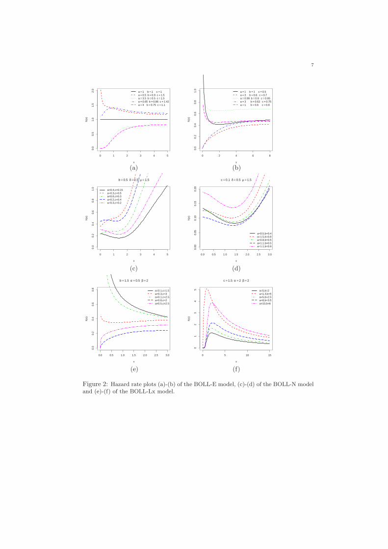
In Figures 1 and 2, we display some plots of the pdf and hrf of the BOLL-E, BOLL-N and BOLL-Lx distributions for selected parameter values. Figure1 reveals that the BOLL-E, BOLL-N and BOLL-Lx densities generate variousshapes such as symmetrical, left-skewed, right-skewed, reversed-J, unimodal andbimodal. Also, Figure 2 shows that these models can produce hazard rate shapessuch as constant, increasing, decreasing, J and upside-down bathtub. This factimplies that the BOLL-G family can be very useful for fitting data sets with variousshapes.

6

0 1 2 3 4 5

0.0

0.2

0.4

0.6

0.8

1.0

x

Den

sity

a = 1 b = 1 c = 1a = 0.5 b = 0.8 c = 1.5a = 3.5 b = 0.5 c = 1.5a = 2.5 b = 0.8 c = 2a = 20 b = 2.5 c = 1.5

0 2 4 6 8

0.0

0.2

0.4

0.6

0.8

x

Den

sity

a = 1 b = 1 c = 0.5a = 50 b = 2.8 c = 0.7a = 3.5 b = 2 c = 0.9a = 15 b = 0.9 c = 0.9a = 25 b = 3.5 c = 0.8

(a) (b)

−4 −2 0 2 4 6

0.00

0.05

0.10

0.15

0.20

0.25

0.30

b = 0.5 δ = 0.5 µ = 1.5

x

Den

sity

a=0.5,c=0.3a=0.4,c=0.2a=0.6,c=0.2a=0.2,c=0.5a=0.3,c=0.6

−2 0 2 4 6

0.0

0.1

0.2

0.3

0.4

a = 1.5 δ = 0.5 µ = 1.5

x

Den

sity

b=0.5,c=0.25b=0.6,c=0.3b=0.45,c=0.2b=1.5,c=0.1b=0.7,c=0.35

(c) (d)

0.0 0.5 1.0 1.5 2.0 2.5

0.0

0.5

1.0

1.5

2.0

b = 1.5 α = 1.5 β = 2

x

Den

sity

a=0.1,c=5a=0.3,c=2.9a=0.4,c=5a=1.5,c=5.5a=4,c=3.5

0.0 0.5 1.0 1.5 2.0 2.5

0.0

0.5

1.0

1.5

2.0

c = 1.5 α = 2 β = 2

x

Den

sity

a=0.1,b=5a=0.3,b=2.9a=0.4,b=5a=1.5,b=5.5a=4,b=3.5

(e) (f)

Figure 1: Density plots (a)-(b) of the BOLL-E model, (c)-(d) of the BOLL-N model and(e)-(f) of the BOLL-Lx model.

7

0 1 2 3 4 5

0.0

0.5

1.0

1.5

2.0

x

h(x)

a = 1 b = 1 c = 1a = 0.5 b = 0.9 c = 1.5a = 3.5 b = 0.5 c = 1.5a = 0.65 b = 0.86 c = 1.42a = 4 b = 0.75 c = 1.1

0 2 4 6 8

0.0

0.2

0.4

0.6

0.8

1.0

x

h(x)

a = 1 b = 1 c = 0.5a = 3 b = 0.6 c = 0.7a = 0.99 b = 0.8 c = 0.85a = 3 b = 0.63 c = 0.75a = 1 b = 0.6 c = 0.8

(a) (b)

0 1 2 3 4 5

0.0

0.2

0.4

0.6

0.8

1.0

b = 0.5 δ = 0.5 µ = 1.5

x

h(x)

a=0.4,c=0.15a=0.3,c=0.5a=0.6,c=0.3a=0.2,c=0.4a=0.3,c=0.2

0.0 0.5 1.0 1.5 2.0 2.5 3.0

0.00

0.05

0.10

0.15

0.20

c = 0.1 δ = 0.5 µ = 1.5

x

h(x)

a=0.5,b=0.4a=1.5,b=0.8a=0.8,b=0.5a=1.1,b=0.5a=1.1,b=0.9

(c) (d)

0.0 0.5 1.0 1.5 2.0 2.5 3.0

0.0

0.2

0.4

0.6

0.8

b = 1.5 α = 0.5 β = 2

x

h(x)

a=0.1,c=1.5a=0.3,c=3a=0.1,c=2.5a=0.8,c=2a=0.5,c=2.5

0 5 10 15

01

23

45

c = 1.5 α = 2 β = 2

x

h(x)

a=5,b=2a=1.3,b=5a=5,b=2.5a=8,b=3.5a=10,b=6

(e) (f)

Figure 2: Hazard rate plots (a)-(b) of the BOLL-E model, (c)-(d) of the BOLL-N modeland (e)-(f) of the BOLL-Lx model.

8

4. Mathematical properties

Here, we present some mathematical properties of the new family of distribu-tions.

4.1. Asymptotics and shapes. The asymptotes of equations (2.3), (2.4) and(2.5) as x → 0 and x →∞ are given by

F (x) ∼ IG(x)c(a, b) as x → 0,

1− F (x) ∼ IG(x)c(b, a) as x →∞,

f(x) ∼ c

B(a, b)g(x)G(x)a c−1 as x → 0,

f(x) ∼ c

B(a, b)g(x)G(x)b c−1 as x →∞,

h(x) ∼ c g(x)G(x)a c−1

1− IG(x)c(a, b)as x → 0,

h(x) ∼ c g(x)G(x)b c−1

IG(x)c(b, a)as x →∞.

The shapes of the density and hazard rate functions can be described analytically.The critical points of the BOLL-G density function are the roots of the equation:

(4.1)g′(x)g(x)

+(ac−1)g(x)G(x)

+(1− bc)g(x)G(x)

−c(a+ b)g(x)G(x)c−1 −G(x)c−1

G(x)c + G(x)c= 0.

There may be more than one root to (4.1). Let λ(x) = d2 log[f(x)]/d x2. We have

λ(x) =g′′(x)g(x)− [g′(x)]2

g(x)2+ (ac− 1)

g′(x)G(x)− g(x)2

G(x)2

+ (1− bc)g′(x)G(x) + g(x)2

G(x)2− c(a + b)g′(x)

G(x)c−1 −G(x)c−1

G(x)c + G(x)c

− c(c− 1)(a + b)g(x)2G(x)c−2 + G(x)c−2

G(x)c + G(x)c

− (a + b)

cg(x)G(x)c−1 −G(x)c−1

G(x)c + G(x)c

2

.

If x = x0 is a root of (4.1) then it corresponds to a local maximum if λ(x) > 0for all x < x0 and λ(x) < 0 for all x > x0. It corresponds to a local minimum ifλ(x) < 0 for all x < x0 and λ(x) > 0 for all x > x0. It refers to a point of inflexionif either λ(x) > 0 for all x 6= x0 or λ(x) < 0 for all x 6= x0.

The critical points of the hrf h(x) are obtained from the equation

g′(x)g(x)

+ (ac− 1)g(x)G(x)

+ (1− bc)g(x)G(x)

− c(a + b)g(x)G(x)c−1 −G(x)c−1

G(x)c + G(x)c

+cg(x)G(x)ac−1G(x)bc−1

B(a, b)G(x)c + G(x)c

a+b

1− I G(x)c

G(x)c+G(x)c(a, b)

= 0.(4.2)

9

There may be more than one root to (4.2). Let τ(x) = d2 log[h(x)]/dx2. We have

τ(x) =g′′(x)g(x)− [g′(x)]2

g(x)2+ (ac− 1)

g′(x)G(x)− g(x)2

G(x)2

+ (1− bc)g′(x)G(x) + g(x)2

G(x)2− c(a + b)g′(x)

G(x)c−1 −G(x)c−1

G(x)c + G(x)c

+ c(c− 1)(a + b)g(x)2G(x)c−2 + G(x)c−2

G(x)c + G(x)c

− (a + b)

cg(x)G(x)c−1 −G(x)c−1

G(x)c + G(x)c

2

+cg′(x)G(x)ac−1G(x)bc−1

G(x)c + G(x)c

a+b

B(a, b)−B(

G(x;ξ)c

G(x;ξ)c+G(x;ξ)c; a, b

)

+c(ac− 1)g(x)2G(x)ac−2G(x)bc−1

G(x)c + G(x)c

a+b

B(a, b)−B(

G(x;ξ)c

G(x;ξ)c+G(x;ξ)c; a, b

)

+c(bc− 1)g(x)2G(x)ac−1G(x)bc−2

G(x)c + G(x)c

a+b

B(a, b)−B(

G(x;ξ)c

G(x;ξ)c+G(x;ξ)c; a, b

)

− c2(a + b)2g(x)G(x)ac−1G(x)bc−1G(x)c−1 −G(x)c−1

G(x)c + G(x)c

a+b+1

B(a, b)−B(

G(x;ξ)c

G(x;ξ)c+G(x;ξ)c; a, b

)

+

cg(x)G(x)ac−1G(x)bc−1

G(x)c + G(x)c

a+b

B(a, b)−B(

G(x;ξ)c

G(x;ξ)c+G(x;ξ)c; a, b

)

2

.

If x = x0 is a root of (4.2) then it refers to a local maximum if τ(x) > 0 for allx < x0 and τ(x) < 0 for all x > x0. It corresponds to a local minimum if τ(x) < 0for all x < x0 and τ(x) > 0 for all x > x0. It gives an inflexion point if eitherτ(x) > 0 for all x 6= x0 or τ(x) < 0 for all x 6= x0.

4.2. Useful expansions. For an arbitrary baseline cdf G(x), a random variableZ has the exp-G distribution (see Section 1) with power parameter c > 0, sayZ ∼exp-G(c), if its pdf and cdf are given by hc(x) = cG(x)c−1 g(x) and Hc(x) =G(x)c, respectively. Some structural properties of the exp-G distributions arestudied by Mudholkar and Srivastava [35], Mudholkar et al. [36], Mudholkar andHutson [34], Gupta et al. [26], Gupta and Kundu [27, 28], Nadarajah and Kotz[39], Nadarajah and Gupta [40, 41] and Nadarajah [37].

We can prove that the cdf (2.3) admits the expansion

F (x) =∞∑

l=0

(−1)l

B(a, b)(a + l)

(b− 1

l

)G(x)c(a+l)

[G(x)c + G(x)c]a+l

=∞∑

l=0

(−1)l

B(a, b)(a + l)

(b− 1

l

) ∑∞k=0 α

(l)k G(x)k

∑∞k=0 β

(l)k G(x)k

.

10

Using the power series for the ratio of two power series, we have

F (x) =∞∑

l=0

(−1)l

B(a, b)(a + l)

(b− 1

l

) ∞∑

k=0

γ(l)k G(x)k,

where (for each l) α(l)k = ak(c(a+l)), β

(l)k = hk(c, a+ l), ak(c(a+ l)) and hk(c, a+ l)

are defined in the Appendix A and γ(l)k is determined recursively as

γ(l)k = γk(a, c) =

1

β(l)0

(α

(l)k − 1

β(l)0

k∑r=1

β(l)r γ

(l)k−r

).

Then, we have

F (x) =∞∑

k=0

bk Hk(x),

where

bk =∞∑

l=0

(−1)l γ(l)k

B(a, b) (a + l)

(b− 1

l

),(4.3)

and Hk(x) = G(x)k denotes the exp-G cdf with power parameter k. So, the densityfunction of X can be expressed as

(4.4) f(x) = f(x; a, b, c, ξ) =∞∑

k=0

bk+1 hk+1(x; ξ),

where hk+1(x) = hk+1(x; ξ) = (k + 1) g(x; ξ)G(x; ξ)k denotes the exp-G densityfunction with power parameter k+1. Hereafter, a random variable having densityfunction hk+1(x) is denoted by Yk+1 ∼ exp-G(k + 1). Equation (4.4) reveals thatthe BOLL-G density function is an infinite mixture of exp-G densities. Thus,some mathematical properties of the new model can be obtained directly fromthose exp-G properties. For example, the ordinary and incomplete moments, andmgf of X can be determined from those quantities of the exp-G distribution.

The formulae derived throughout the paper can be easily handled in most sym-bolic computation software platforms such as Maple, Mathematica and Matlab.These platforms have currently the ability to deal with analytic expressions offormidable size and complexity. Established explicit expressions to calculate sta-tistical measures can be more efficient than computing them directly by numericalintegration. The infinity limit in these sums can be substituted by a large positiveinteger such as 20 or 30 for most practical purposes.

4.3. Quantile function. The qf of X, say x = Q(u) = F−1(u), can be obtainedby inverting (2.3). Let z = Qa,b(u) be the beta qf. Then,

x = Q(u) = QG

[Qa,b(u)]

1c

[Qa,b(u)]1c + [1−Qa,b(u)]

1c

.

11

It is possible to obtain some expansions for Qa,b(u) from the Wolfram websitehttp://functions.wolfram.com/06.23.06.0004.01 such as

z = Qa,b(u) =∞∑

i=0

ei ui/a,

where ei = [aB(a, b)]1/a di and d0 = 0, d1 = 1, d2 = (b− 1)/(a + 1),

d3 =(b− 1) (a2 + 3ab− a + 5b− 4)

2(a + 1)2(a + 2),

d4 = (b− 1)[a4 + (6b− 1)a3 + (b + 2)(8b− 5)a2 + (33b2 − 30b + 4)a+ b(31b− 47) + 18]/[3(a + 1)3(a + 2)(a + 3)], . . .

The effects of the shape parameters a, b and c on the skewness and kurtosis ofX can be based on quantile measures. The Bowley skewness (Kenney and Keeping[30]) is one of the earliest skewness measures defined by the average of the quartilesminus the median, divided by half the interquartile range, namely

B =Q

(34

)+ Q

(14

)− 2Q(

12

)

Q(

34

)−Q(

14

) .

Since only the middle two quartiles are considered and the outer two quartiles areignored, this adds robustness to the measure. The Moors kurtosis (Moors [33]) isbased on octiles

M =Q

(38

)−Q(

18

)+ Q

(78

)−Q(

58

)

Q(

68

)−Q(

28

) .

These measures are less sensitive to outliers and they exist even for distributionswithout moments.

In Figure 3, we plot the measures B and M for the BOLL-N and BOLL-Lxdistributions. The plots indicate the variability of these measures on the shapeparameters.

4.4. Moments. We assume that Y is a random variable having the baseline cdfG(x). The moments of X can be obtained from the (r, k)th probability weightedmoment (PWM) of Y defined by Greenwood et al. [23] as

τr,k = E[Y r G(Y )k] =∫ ∞

−∞xr G(x)k g(x)dx.

The PWMs are used to derive estimators of the parameters and quantiles of gen-eralized distributions. The method of estimation is formulated by equating thepopulation and sample PWMs. These moments have low variance and no severebiases, and they compare favorably with estimators obtained by maximum like-lihood. The maximum likelihood method is adopted in Section 6.1 since it iseasier to estimate the BOLL-G parameters because of several computer routinesavailable in widely known softwares. The maximum likelihood estimators (MLEs)enjoy desirable properties and can be used when constructing confidence intervalsand regions and also in test statistics.

12

0 1 2 3 4 5

−0.

4−

0.2

0.0

0.2

0.4

µ = 1.5 δ = 1

c

Ske

wne

ss

a=0.9,b=0.5a=0.8,b=1.5a=3,b=0.9a=0.9,b=0.7a=2.5,b=1.2

0 1 2 3 4 5

−1.

0−

0.5

0.0

0.5

1.0

1.5

β = 2

α

Ske

wne

ss

a=0.8,b=0.6,c=0.4a=0.5,b=0.5,c=2.5a=2.5,b=2,c=0.5a=5,b=1.5,c=2.5a=0.5,b=5,c=3

(a) (b)

0 1 2 3 4 5

1.15

1.20

1.25

1.30

µ = 1.5 δ = 1

c

Kur

tosi

s

a=0.8,b=0.3a=0.8,b=1.5a=3,b=0.9a=0.7,b=0.3a=2.5,b=1.2

0 1 2 3 4 5

24

68

10

β = 2

α

Kur

tosi

sa=0.8,b=0.6,c=0.4a=0.5,b=0.5,c=2.5a=2.5,b=1.5,c=0.5a=5,b=1.5,c=1.5a=0.5,b=2,c=1.3

(c) (d)

Figure 3: Skewness (a) and (b) and kurtosis (c) and (d) of X based on the quantiles forthe BOLL-N and BOLL-Lx distributions, respectively.

We can write from equation (4.4)

µ′r = E(Xr) =∞∑

k=0

(k + 1) bk+1 τr,k,(4.5)

where τr,k =∫ 1

0QG(u)r ukdu can be computed at least numerically from any

baseline qf.Thus, the moments of any BOLL-G distribution can be expressed as an infi-

nite weighted sum of the baseline PWMs. We now provide the PWMs for threedistributions discussed in Section 3. For the BOLL-N and BOLL-Ga distributionsdiscussed in subsections 3.2 and 3.5, the quantities τr,k can be expressed in termsof the Lauricella functions of type A (see Exton [16] and Trott [52]) defined by

F(n)A (a; b1, . . . , bn; c1, . . . , cn;x1, . . . , xn) =∞∑

m1=0

. . .

∞∑mn=0

(a)m1+...+mn(b1)m1 . . . (bn)mn

(c1)m1 . . . (cn)mn

xm11 . . . xmn

n

m1! . . . mn!,

13

where (a)i = a(a + 1) . . . (a + i− 1) is the ascending factorial (with the conventionthat (a)0 = 1).

In fact, Cordeiro and Nadarajah [11] determined τr,k for the standard normaldistribution as

τr,k = 2r/2 π−(k+1/2)k∑

l=0(r+k−l) even

(k

l

)2−l πl Γ

(r + k − l + 1

2

)×

F(k−l)A

(r + k − l + 1

2;12, . . . ,

12;32, . . . ,

32;−1, . . . ,−1

).

This equation holds when r+k− l is even and it vanishes when r+k− l is odd. So,any BOLL-N moment can be expressed as an infinite weighted linear combinationof Lauricella functions of type A.

For the gamma distribution, the quantities τr,k can be expressed from equation(9) of Cordeiro and Nadarajah [11] as

τr,k =Γ(r + (k + 1)α)αk βr Γ(α)k+1

F(k)A (r + (k + 1)α; α, . . . , α; α + 1, . . . , α + 1,−1, . . . ,−1).

Finally, for the BOLL-W distribution, the quantities τr,k are given by

τr,k =Γ(r/β + 1)

αr/β

k∑s=0

(−1)s

(s + 1)r/β+1

(k

s

).

4.5. Generating function. Here, we provide two formulae for the mgf M(s) =E(es X) of X. The first formula for M(s) comes from equation (4.4) as

M(s) =∞∑

k=0

bk+1 Mk+1(s),(4.6)

where Mk+1(s) is the exp-G generating function with power parameter k + 1.Equation (4.6) can also be expressed as

M(s) =∞∑

k=0

(k + 1) bk+1 ρk(s),(4.7)

where the quantity ρk(s) =∫ 1

0exp [sQG(u)] ukdu can be computed numerically.

4.6. Mean deviations. Incomplete moments are useful for measuring inequality,for example, the Lorenz and Bonferroni curves and Pietra and Gini measures ofinequality all depend upon the incomplete moments of the distribution. The nthincomplete moment of X is defined by mn(y) =

∫ y

−∞ xn f(x)dx. Here, we proposetwo methods to determine the incomplete moments of the new family. First, thenth incomplete moment of X can be expressed as

mn(y) =∞∑

k=0

bk+1

∫ G(y; ξ)

0

QG(u)n uk du.(4.8)

The integral in (4.8) can be computed at least numerically for most baseline dis-tributions.

14

The mean deviations about the mean (δ1 = E(|X−µ′1|)) and about the median(δ2 = E(|X −M |)) of X are given by

δ1 = 2µ′1 F (µ′1)− 2m1 (µ′1) and δ2 = µ′1 − 2m1(M),(4.9)

respectively, where M = Q(0.5) is the median of X, µ′1 = E(X) comes from equa-tion (4.5), F (µ′1) can easily be calculated from (2.3) and m1(z) =

∫ z

−∞ x f(x)dx isthe first incomplete moment.

Next, we provide two alternative ways to compute δ1 and δ2. A general equationfor m1(z) can be derived from equation (4.4) as

m1(z) =∞∑

k=0

bk+1 Jk+1(z),(4.10)

where

Jk+1(z) =∫ z

−∞xhk+1(x)dx.

Equation (4.10) is the basic quantity to compute the mean deviations in (4.9).A simple application of (4.10) refers to the BOLL-W model. The exponentiatedWeibull density function (for x > 0) with power parameter k+1, shape parameterα and scale parameter β, is given by

hk+1(x) = (k + 1) α βα xα−1 exp −(βx)α [1− exp −(βx)α]k ,

and then

Jk+1(z) = c (k + 1) βα∞∑

r=0

(−1)r

(k

r

) ∫ z

0

xα exp −(r + 1)(βx)α dx.

The last integral reduces to the incomplete gamma function and then

Jk+1(z) = β−1∞∑

r=0

(−1)r (k + 1)(kr

)

(r + 1)1+α−1 γ(1 + α−1, (r + 1)(βz)α

).

A second general formula for m1(z) can be derived by setting u = G(x) in (4.4)

m1(z) =∞∑

k=0

(k + 1) bk+1 Tk(z),

where Tk(z) =∫ G(z)

0QG(u)ukdu.

The main application of the first incomplete moment refers to the Bonferroniand Lorenz curves which are very useful in economics, reliability, demography,insurance and medicine. For a given probability π, applications of these equationscan be addressed to obtain these curves defined by B(π) = m1(q)/(π µ′1) andL(π) = m1(q)/µ′1, respectively, where q = Q(π) is calculated from the parent qf.

4.7. Entropies. An entropy is a measure of variation or uncertainty of a randomvariable X. Two popular entropy measures are the Renyi [43] and Shannon [45].The Renyi entropy of a random variable with pdf f(x) is defined by

IR(γ) =1

1− γlog

(∫ ∞

0

fγ(x)dx

),

15

for γ > 0 and γ 6= 1. The Shannon entropy of a random variable X is given byIS = E − log [f(X)]. It is the special case of the Renyi entropy when γ ↑ 1.Direct calculation yields

IS = − log[

c

B(a, b)

]− E log [g(X; ξ)]+ (1− ac) E log [G(x; ξ)]

+ (1− bc) Elog

[G(x; ξ)

]+ (a + b) E

log

[G(x; ξ)c + G(x; ξ)c

].

First, we define and compute

A(a1, a2, a3; a) =∫ 1

0

ua1(1− u)a2

[ua + (1− u)a]a3 du

=∞∑

i=0

(−1)i

(a2

i

) ∫ 1

0

ua1+i

[ua + (1− u)a]a3 du

=∞∑

i=0

(−1)i

(a2

i

) ∫ 1

0

∑∞k=0 δ1,kuk

∑∞k=0 δ2,k uk

du

=∞∑

i=0

(−1)i

(a2

i

) ∫ 1

0

∞∑

k=0

δ3,kuk

=∞∑

i=0

(−1)i δ3,k

(k + 1)

(a2

i

),

where δ1,k = ak(a1 + i), δ2,k = hk(a, a3) and

δ3,k =1

δ2,0

(δ1,k − 1

δ2,0

k∑r=1

δ2,r δ3,k−r

).

After some algebraic manipulations, we obtain:

4.1. Theorem. Let X be a random variable with pdf (2.4). Then,

E log [G(X)] =c

B(a, b)∂

∂tA(a c + t− 1, b c− 1, a + b; c)

∣∣∣t=0

,

Elog

[G(X)

]=

c

B(a, b)∂

∂tA(a c− 1, b c + t− 1, a + b; c)

∣∣∣t=0

,

EG(x; ξ)a + G(X; ξ)a

=

c

B(a, b)∂

∂tA(a c− 1, b c− 1, a + b− t; c)

∣∣∣t=0

.

The simplest formula for the entropy of X is given by

IS = − log[ c

B(a, b)

]− E log [g(X; ξ)]

+c (1− a c)B(a, b)

∂

∂tA(a c + t− 1, b c− 1, a + b; c)

∣∣∣t=0

+c (1− b c)B(a, b)

∂

∂tA(a c− 1, b c + t− 1, a + b; c)

∣∣∣t=0

+c (a + b)B(a, b)

∂

∂tA(a c− 1, b c− 1, a + b− t; c)

∣∣∣t=0

.

16

After some algebraic developments, we have an alternative expression for IR(γ):

IR(γ) =γ

1− γlog

[c

B(a, b)

]+

11− γ

log

∞∑

i,k=0

ti,k EVk(gγ−1[G−1(Y )])

.

Here, Vk has a beta distribution with parameters k + 1 and one,

ti,k =(−1)i γ3,k(a, b, c, i)

(k + 1)

(c(a− 1)

i

),

γ1,k = ak

((a c− 1)γ + i

), γ2,k = hk

(c, (a + b)γ

)

and

γ3,k =1

γ2,0

(γ1,k − 1

γ2,0

k∑r=1

γ2,rγ3,k−r

),

where ak((a c − 1)γ + i) and hk

(c, (a + b)γ

)are defined in equation (8.6) given

in Appendix A.

4.8. Order statistics. Order statistics make their appearance in many areas ofstatistical theory and practice. Suppose X1, . . . , Xn is a random sample from theBOLL-G family of distributions. We can write the density of the ith order statistic,say Xi:n, as

fi:n(x) = K f(x)F i−1(x) 1− F (x)n−i = K

n−i∑

j=0

(−1)j

(n− i

j

)f(x) F (x)j+i−1,

where K = n!/[(i− 1)! (n− i)!].Following similar algebraic developments of Nadarajah et al. [38], we can write

the density function of Xi:n as

fi:n(x) =∞∑

r,k=0

mr,k hr+k+1(x),(4.11)

where hr+k(x) denotes the exp-G density function with power parameter r +k +1(for r, k ≥ 0)

mr,k =n! (r + 1) (i− 1)! br+1

(r + k + 1)

n−i∑

j=0

(−1)j fj+i−1,k

(n− i− j)! j!,

and bk is defined in equation (4.3). The quantities fj+i−1,k can be obtained recur-sively by fj+i−1,0 = bj+i−1

0 and

fj+i−1,k = (k b0)−1

k∑m=1

[m(j + i)− k] bm fj+i−1,k−m, k ≥ 1.

Equation (4.11) is the main result of this section. It reveals that the pdf of theBOLL-G order statistics is a linear combination of exp-G density functions. So,several mathematical quantities of the BOLL-G order statistics such as ordinary,incomplete and factorial moments, mgf, mean deviations and several others canbe determined from those quantities of the exp-G distribution.

17

5. Characterizations of the new family based on two truncatedmoments

The problem of characterizing distributions is an important problem whichhas attracted the attention of many researchers recently. An investigator will,generally, be interested to know if their chosen model fits the requirements of aparticular distribution. Hence, one will depend on the characterizations of thisdistribution which provide conditions under which one can check to see if theunderlying distribution is indeed that particular distribution. Various characteri-zations of distributions have been established in many different directions. In thissection, we present characterizations of the BOLL-G distribution based on a sim-ple relationship between two truncated moments. Our characterization results willemploy a theorem due to Glanzel [24] (Theorem 5.1, below). The advantage of thecharacterizations given here is that the cdf F is not required to have a closed-formand is given in terms of an integral whose integrand depends on the solution of afirst order differential equation, which can serve as a bridge between probabilityand differential equation. We believe that other characterizations of the BOLL-Gfamily may not be possible.

5.1. Theorem. Let (Ω, Σ,P) be a given probability space and let H = [a, b] be aninterval for some a < b (a = −∞, b = ∞ might as well be allowed). Let X : Ω → Hbe a continuous random variable with distribution function F (x) and let q1 and q2

be two real functions defined on H such thatE [q1(X) |X ≥ x] = E [q2(X) |X ≥ x] η(x), x ∈ H,

is defined with some real function η. Consider that q1, q2 ∈ C1(H), η ∈ C2(H)and F (x) is twice continuously differentiable and strictly monotone function onthe set H. Further, we assume that the equation q2η = q1 has no real solution inthe interior of H. Then, F is uniquely determined by the functions q1, q2 and η,particularly

F (x) =∫ x

a

C

∣∣∣∣η′ (u)

η (u) q2 (u)− q1 (u)

∣∣∣∣ e−s(u) du ,

where the function s is a solution of the differential equation s′ = η′ q2η q2−q1

and C

is a constant chosen to make∫

HdF = 1.

We have to mention that this kind of characterization based on the ratio of trun-cated moments is stable in the sense of weak convergence. In particular, let usassume that there is a sequence Xn of random variables with distribution func-tions Fn such that the functions q1,n, q2,n and ηn (n ∈ N) satisfy the conditionsof Theorem 5.1 and let q1,n → q1, q2,n → q2 for some continuously differentiablereal functions q1 and q2. Finally, let X be a random variable with distribution F .Under the condition that q1,n (X) and q2,n (X) are uniformly integrable and thefamily Fn is relatively compact, the sequence Xn converges to X in distributionif and only if ηn converges to η, where

η (x) =E [q1 (X) |X ≥ x]E [q2 (X) |X ≥ x]

.

18

5.2. Remark. (a) In Theorem 5.1, the interval H need not be closed since thecondition is only on the interior of H.(b)Clearly, Theorem 5.1 can be stated in terms of two functions q1 and η by takingq2 (x) = 1, which will reduce the condition in Theorem 5.1 to E [q1 (X) |X ≥ x] =η (x). However, adding an extra function will give a lot more flexibility, as far asits application is concerned.

5.3. Proposition. Let X : Ω → R be a continuous random variable and letq1 (x) = q2 (x) G (x; ξ)ac and q2 (x) =

G (x; ξ)c + G (x; ξ)c−(a+b)

G (x; ξ)1−bc forx ∈ R. The pdf of X is (2.4) if and only if the function η defined in Theorem 5.1has the form

η (x) =12

[1 + G (x; ξ)ac] , x ∈ R.

Proof. If X has pdf (2.4), then

[1− F (x)]E [q2 (X) |X ≥ x] =1

aB (a, b)[1−G (x; ξ)ac] , x ∈ R

and

[1− F (x)]E [q1 (X) |X ≥ x] =1

2aB (a, b)

[1−G (x; ξ)2ac

], x ∈ R.

Finally,

η (x) q2 (x)− q1 (x) =12q2 (x) [1−G (x; ξ)ac] > 0, for x ∈ R.

Conversely, if η is given as above, then

s′ (x) =η′ (x) q2 (x)

η (x) q2 (x)− q1 (x)=

a c g (x) G (x; ξ)ac−1

[1−G (x; ξ)ac], x ∈ R,

and hence

s (x) = − log [1−G (x; ξ)ac] , x ∈ R.

Now, in view of Theorem 5.1, X has pdf (2.4). ¤

5.4. Corollary. Let X : Ω → R be a continuous random variable and let q2 (x) beas in Proposition 5.3. The pdf of X is (2.4) if and only if there exist functions q1

and η defined in Theorem 5.1 satisfying the differential equation

η′(x) q2(x)η(x) q2(x)− q1(x)

=a c g(x)G(x; ξ)ac−1

[1−G(x; ξ)ac], x ∈ R.

5.5. Remark. (a) The general solution of the differential equation in Corollary5.4 is

η(x) = [1−G(x; ξ)ac]−1

[−

∫a c g(x)G(x; ξ)ac−) q1(x) q2(x)−1 dx + D

],

for x ∈ R, where D is a constant. One set of appropriate functions is given inProposition 5.3 with D = 1/2.

19

(b) Clearly there are other triplets of functions (q1, q2, η) satisfying the condi-tions of Theorem 5.1, e.g.,

q1(x) = q2(x)G(x; ξ)bc

and

q2(x) =[G(x; ξ)c + G(x; ξ)c

]−(a+b)G(x; ξ)1−ac, x ∈ R.

Then, η(x) = 12 G(x; ξ)bc and s′(x) = η′(x) q2(x)

η(x) q2(x)−q1(x) = b c g(x)G(x)−1, x ∈ R.

6. Different methods of estimation

Here, we discuss parameter estimation using the methods of maximum likeli-hood and of minimum spacing distance estimator proposed by Torabi [48].

6.1. Maximum likelihood estimation. We consider the estimation of the un-known parameters of this family from complete samples only by the method ofmaximum likelihood. Let x1, . . . , xn be observed values from the BOLL-G distri-bution with parameters a, b, c and ξ. Let Θ = (a, b, c, ξ)> be the r× 1 parametervector. The total log-likelihood function for Θ is given by

`n = n log(c)− n log[B(a, b)] +n∑

i=1

log[g(xi; ξ)] + (ac− 1)n∑

i=1

log[G(xi; ξ)]

+ (bc− 1)n∑

i=1

log[G(xi; ξ)]− (a + b)n∑

i=1

logG(xi; ξ)c + G(xi; ξ)c

.(6.1)

The log-likelihood function can be maximized either directly by using the R(AdequacyModel or Maxlik) (see R Development Core Team [42]), SAS (PROCNLMIXED), Ox program (sub-routine MaxBFGS) (see Doornik [14]), Limited-Memory quasi-Newton code for bound-constrained optimization (L-BFGS-B) orby solving the nonlinear likelihood equations obtained by differentiating (6.1).

Let Un(Θ) = (∂`n/∂a, ∂`n/∂b, ∂`n/∂c, ∂`n/∂ξ)> be the score function. Itscomponents are given by

∂`n

∂a= −nψ(a) + nψ(a + b) + c

n∑

i=1

log[G(xi; ξ)]−n∑

i=1

logG(xi; ξ)c + G(xi; ξ)c

,

∂`n

∂b= −nψ(b) + nψ(a + b) + c

n∑

i=1

log[G(xi; ξ)]−n∑

i=1

logG(xi; ξ)c + G(xi; ξ)c

,

∂`n

∂c=

n

c+ a

n∑

i=1

log[G(xi; ξ)] + b

n∑

i=1

log[G(xi; ξ)]

−(a + b)n∑

i=1

G(xi; ξ)c log[G(xi; ξ)] + G(xi; ξ)c log[G(xi; ξ)]G(xi; ξ)c + G(xi; ξ)c

,

∂`n

∂ξ=

n∑

i=1

g(xi; ξ)(ξ)

g(xi; ξ)+ (ac− 1)

n∑

i=1

G(xi; ξ)(ξ)

G(xi; ξ)+ (1− bc)

n∑

i=1

G(xi; ξ)(ξ)

G(xi; ξ)

20

−c(a + b)n∑

i=1

G(xi; ξ)(ξ)G(xi; ξ)c−1 − G(xi; ξ)c−1

G(xi; ξ)c + G(xi; ξ)c,

where h(ξ)(·) means the derivative of the function h with respect to ξ.For interval estimation and hypothesis tests, we can use standard likelihood

techniques based on the observed information matrix, which can be obtained fromthe authors upon request.

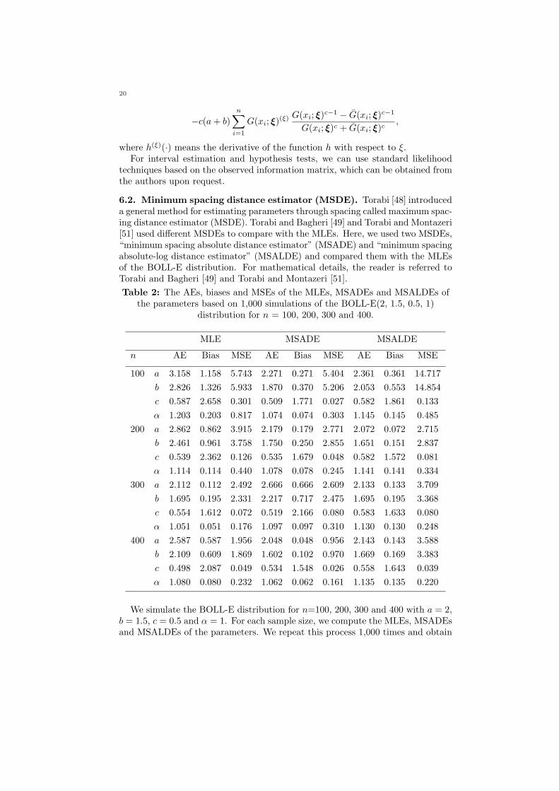
6.2. Minimum spacing distance estimator (MSDE). Torabi [48] introduceda general method for estimating parameters through spacing called maximum spac-ing distance estimator (MSDE). Torabi and Bagheri [49] and Torabi and Montazeri[51] used different MSDEs to compare with the MLEs. Here, we used two MSDEs,“minimum spacing absolute distance estimator” (MSADE) and “minimum spacingabsolute-log distance estimator” (MSALDE) and compared them with the MLEsof the BOLL-E distribution. For mathematical details, the reader is referred toTorabi and Bagheri [49] and Torabi and Montazeri [51].Table 2: The AEs, biases and MSEs of the MLEs, MSADEs and MSALDEs of

the parameters based on 1,000 simulations of the BOLL-E(2, 1.5, 0.5, 1)distribution for n = 100, 200, 300 and 400.

MLE MSADE MSALDE

n AE Bias MSE AE Bias MSE AE Bias MSE

100 a 3.158 1.158 5.743 2.271 0.271 5.404 2.361 0.361 14.717b 2.826 1.326 5.933 1.870 0.370 5.206 2.053 0.553 14.854c 0.587 2.658 0.301 0.509 1.771 0.027 0.582 1.861 0.133α 1.203 0.203 0.817 1.074 0.074 0.303 1.145 0.145 0.485

200 a 2.862 0.862 3.915 2.179 0.179 2.771 2.072 0.072 2.715b 2.461 0.961 3.758 1.750 0.250 2.855 1.651 0.151 2.837c 0.539 2.362 0.126 0.535 1.679 0.048 0.582 1.572 0.081α 1.114 0.114 0.440 1.078 0.078 0.245 1.141 0.141 0.334

300 a 2.112 0.112 2.492 2.666 0.666 2.609 2.133 0.133 3.709b 1.695 0.195 2.331 2.217 0.717 2.475 1.695 0.195 3.368c 0.554 1.612 0.072 0.519 2.166 0.080 0.583 1.633 0.080α 1.051 0.051 0.176 1.097 0.097 0.310 1.130 0.130 0.248

400 a 2.587 0.587 1.956 2.048 0.048 0.956 2.143 0.143 3.588b 2.109 0.609 1.869 1.602 0.102 0.970 1.669 0.169 3.383c 0.498 2.087 0.049 0.534 1.548 0.026 0.558 1.643 0.039α 1.080 0.080 0.232 1.062 0.062 0.161 1.135 0.135 0.220

We simulate the BOLL-E distribution for n=100, 200, 300 and 400 with a = 2,b = 1.5, c = 0.5 and α = 1. For each sample size, we compute the MLEs, MSADEsand MSALDEs of the parameters. We repeat this process 1,000 times and obtain

21

the average estimates (AEs), biases and mean square error (MSEs). The results arereported in Table 2. From the figures in this table, we note that the performancesof the MLEs and MSADEs are better than MSALDEs.

7. Applications

In this section, we provide two applications to real data to illustrate the im-portance of the BOLL-G family through the special models: BOLL-E, BOLL-Nand BOLL-Lx. The MLEs of the parameters are computed and the goodness-of-fitstatistics for these models are compared with other competing models.

7.1. Data set 1: Strength of glass fibres. The first data set represents thestrength of 1.5 cm glass fibres, measured at National physical laboratory, England(see, Smith and Naylor [46]). The data are: 0.55, 0.93, 1.25, 1.36, 1.49, 1.52, 1.58,1.61, 1.64, 1.68, 1.73, 1.81, 2.00, 0.74, 1.04, 1.27, 1.39, 1.49, 1.53, 1.59, 1.61, 1.66,1.68, 1.76, 1.82, 2.01, 0.77, 1.11, 1.28, 1.42, 1.50, 1.54, 1.60, 1.62, 1.66, 1.69, 1.76,1.84, 2.24, 0.81, 1.13, 1.29, 1.48, 1.50, 1.55, 1.61, 1.62, 1.66, 1.70, 1.77, 1.84, 0.84,1.24, 1.30, 1.48, 1.51, 1.55, 1.61, 1.63, 1.67, 1.70, 1.78, 1.89.

We fit the BOLL-E, BOLL-N, McDonald-Normal (McN) (Cordeiro et al. [9]),beta-normal (BN) (Famoye et al. [17]) and beta-exponential (BE) (Nadarajah andKotz [39]) models to data set 1 and also compare them through seven goodness-of-fit statistics. The densities of the McN, BN and BE models are, respectively,given by:

McN : fMcN(x; a, b, c, µ, σ) = cσ B(a,b) φ

(x−µ

σ

)Φ

(x−µ

σ

)ac−1[1− Φ

(x−µ

σ

)c]b−1

,

µ ∈ <, a, b, c, σ > 0,

BN : fBN(x; a, b, µ, σ) = 1σ B(a,b)φ

(x−µ

σ

)Φ

(x−µ

σ

)a−1 [1− Φ

(x−µ

σ

)]b−1,

µ ∈ <, a, b, σ > 0,

BE : fBE(x; a, b, α) = αB(a,b) e−α b x (1− e−α x)a−1

, a, b, α > 0.

7.2. Data set 2: Bladder cancer patients. The second data set representsthe uncensored remission times (in months) of a random sample of 128 bladdercancer patients reported in Lee and Wang [31]. The data are: 0.08, 2.09, 3.48,4.87, 6.94, 8.66, 13.11, 23.63, 0.20, 2.23, 3.52, 4.98, 6.97, 9.02, 13.29, 0.40, 2.26,3.57, 5.06, 7.09, 9.22, 13.80, 25.74, 0.50, 2.46, 3.64, 5.09, 7.26, 9.47, 14.24, 25.82,0.51, 2.54, 3.70, 5.17, 7.28, 9.74, 14.76, 26.31, 0.81, 2.62, 3.82, 5.32, 7.32, 10.06,14.77, 32.15, 2.64, 3.88, 5.32, 7.39, 10.34, 14.83, 34.26, 0.90, 2.69, 4.18, 5.34, 7.59,10.66, 15.96, 36.66, 1.05, 2.69, 4.23, 5.41, 7.62, 10.75, 16.62, 43.01, 1.19, 2.75, 4.26,5.41, 7.63, 17.12, 46.12, 1.26, 2.83, 4.33,5.49, 7.66, 11.25, 17.14, 79.05, 1.35, 2.87,5.62, 7.87, 11.64, 17.36, 1.40, 3.02, 4.34, 5.71, 7.93, 11.79, 18.10, 1.46, 4.40, 5.85,8.26, 11.98, 19.13, 1.76, 3.25, 4.50, 6.25, 8.37, 12.02, 2.02, 3.31, 4.51, 6.54, 8.53,12.03, 20.28, 2.02, 3.36, 6.76, 12.07, 21.73, 2.07, 3.36, 6.93, 8.65, 12.63, 22.69.

We fit the BOLL-E, BOLL-Lx, McDonald-Lomax (McLx) and beta-Lomax(BLx) (Lemonte and Cordeiro [32]) and BE models to these data and also compare

22

their goodness-of-fit statistics. The densities of the McLx and BLx models are,respectively, given by

McLx : fMcLx(x; a, b, c, α, β) = c αβ B(a,b)

[1 +

(xβ

)]−(α+1)

×

1−[1 +

(xβ

)]−αac−1 [1−

1−

[1 +

(xβ

)]−αc]b−1

,

a, b, c, α, β > 0,

BLx : fBLx(x; a, b, α, β) = αβ B(a,b)

[1 +

(xβ

)]−(αb+1)1−

[1 +

(xβ

)]−αa−1

×[1−

1−

[1 +

(xβ

)]−αa]b−1

, a, b, α, β > 0.

For all models, the MLEs are computed using the Limited-Memory Quasi-NewtonCode for Bound-Constrained Optimization (L-BFGS-B). Further, the log-likelihoodfunction evaluated at the MLEs (ˆ), Akaike information criterion (AIC), consis-tent Akaike information criterion (CAIC), Bayesian information criterion (BIC),Hannan-Quinn information criterion (HQIC), Anderson-Darling (A∗), Cramer–von Mises (W ∗) and Kolmogorov-Smirnov (K-S) statistics are calculated to com-pare the fitted models. The statistics A∗ and W ∗ are defined by Chen and Bal-akrishnan [8]. In general, the smaller the values of these statistics, the better thefit to the data. The required computations are carried out in R-language.

Table 3: MLEs and their standard errors (in parentheses) for the first data set.

Distribution a b c µ σ α

BOLL-E 0.0698 0.1834 50.4548 - - 0.4118(0.0931) (0.2712) (66.9766 - - (0.0125)

BOLL-N 0.0358 0.0764 34.7642 1.6597 0.6056 -(0.0660) (0.1384) (65.6410) (0.0381) (0.5323) -

McN 0.5298 17.2226 1.2924 2.3850 0.4773 -(0.5249) (48.8078) (6.2595) (1.8112) (0.9820) -

BN 0.5836 21.9402 - 2.5679 0.4658 -(0.6444) (79.8234) - (1.3451) (0.4546) -

BE 17.4548 38.3856 - - - 0.2514(3.1323) (65.8297) - - - (0.3684)

Table 4: The statistics ˆ, AIC, CAIC , BIC , HQIC, A∗ and W ∗ for the first data set.

Distribution ˆ AIC CAIC BIC HQIC A∗ W ∗

BOLL-E −10.4852 28.9703 29.6599 37.5429 32.3419 0.3923 0.0681BOLL-N −9.9976 29.9953 31.0479 40.7110 34.2098 2.0245 0.2858McN −14.0577 38.1154 39.1680 48.8311 42.3299 0.9289 0.1659BN −14.0560 36.1119 36.8016 44.6845 39.4836 0.9179 0.1637BE −24.0256 54.0511 54.4579 60.4805 56.5798 3.1307 0.5708

23

Table 5: The K-S statistics and p-values for the first data set.

Distribution K-S p-value (K-S)

BOLL-E 0.1126 0.4013BOLL-N 0.0928 0.6496McN 0.1369 0.1886BN 0.1356 0.1973BE 0.2168 0.0053

Table 6: MLEs and their standard errors (in parentheses) for the second data set.

Distribution a b c α β

BOLL-E 0.2772 0.1548 3.7895 0.1563 -(0.2529) (0.1441) (3.1996) (0.0413) -

BOLL-Lx 0.4507 0.3046 2.5267 8.5700 57.6246(0.4279) (0.3573) (2.0183) (14.4135) (88.4252)

McLx 1.5052 5.9638 2.0608 0.7177 10.9267(0.2831) (30.1616) (2.9944) (3.0698) (16.6896)

BLx 1.5882 12.0014 - 0.3859 20.4693(0.2830) (319.2372) - (10.0697) (14.0657)

BE 1.3781 0.2543 - 0.4595 -(0.2162) (0.0251) - (0.0028) -

Table 7: The statistics ˆ, AIC, CAIC , BIC , HQIC, A∗ and W ∗ for the second data set.

Distribution ˆ AIC CAIC BIC HQIC A∗ W ∗

BOLL-E −409.8323 827.6646 827.9898 839.0727 832.2998 1.5745 0.2022BOLL-Lx −409.2256 828.4513 828.9431 842.7115 834.2453 0.0800 0.0126McLx −409.9128 829.8256 830.3174 844.0858 835.6196 0.1688 0.0254BLx −410.0813 828.1626 828.4878 839.5708 832.7978 0.1917 0.0285BE −412.1016 830.2033 830.3968 838.7594 833.6797 0.5475 0.0896

Table 8: The K-S statistics and p-values for the second data set.

Distribution K-S p-value (K-S)

BOLL-E 0.0295 0.9999BOLL-Lx 0.0341 0.9984McLx 0.0391 0.9896BLx 0.0407 0.9840BE 0.0688 0.5793

Tables 3 and 6 list the MLEs and their corresponding standard errors (in paren-theses) of the parameters. The values of the model selection statistics AIC, CAIC,BIC, HQIC, A∗, W ∗ and K-S are listed in Tables 4-5 and 7-8. We note from Ta-bles 4 and 5 that the BOLL-E and BOLL-N models have the lowest values of theAIC, CAIC, BIC, HQIC, W ∗ and K-S statistics (for the first data set) among thefitted McN, BN and BE models, thus suggesting that the BOLL-E and BOLL-Nmodels provide the best fits, and therefore could be chosen as the most adequatemodels for the first data set. The histogram of these data and the estimated pdfsand cdfs of the BOLL-E and BOLL-N models and their competitive models aredisplayed in Figure 4. Similarly, it is also evident from the results in Tables 7 and8 that the BOLL-E and BOLL-Lx models give the lowest values for the ˆ, AIC,

24

x

Den

sity

0.5 1.0 1.5 2.0

0.0

0.5

1.0

1.5

2.0

2.5

BOLLNBOLLEMcNBNBE

0.5 1.0 1.5 2.0

0.0

0.2

0.4

0.6

0.8

1.0

x

cdf

BOLLNBOLLEMcNBNBE

(a) Estimated pdfs (b) Estimated cdfs

Figure 4: Plots (a) and (b) of the estimated pdfs and cdfs of the BOLL-E and BOLL-Nand other competitive models.

x

Den

sity

0 20 40 60 80

0.00

0.02

0.04

0.06

0.08

0.10 BOLLLx

BOLLEMcLxBLxBE

0 20 40 60 80

0.0

0.2

0.4

0.6

0.8

1.0

x

cdf

BOLLNBOLLEMcLxBLxBE

(a) Estimated pdfs (b) Estimated cdfs

Figure 5: Plots (a) and (b) of the estimated pdfs and cdfs of the BOLL-E and BOLL-Lxmodels and other competitive models.

CAIC, BIC, HQIC, A∗, W ∗ and K-S statistics (for the second data set) among thefitted McLx, BLx, KwLx and Lx distributions. Thus, the BOLL-E and BOLL-Lxmodels can be chosen as the best models. The histogram of the second data setand the estimated pdfs and cdfs of the BOLL-E and BOLL-Lx models and othercompetitive models are displayed in Figure 5.

It is clear from the figures in Tables 4-5 and 7-8, and Figures 4 and 5 that theBOLL-E, BOLL-N and BOLL-Lx models provide the best fits to these two datasets as compared to other models.

8. Concluding remarks

The generalized continuous univariate distributions have been widely studiedin the literature. We propose a new class of distributions called the beta odd log-logistic-G family. We study some of its structural properties including an expan-sion for its density function and explicit expressions for the moments, generatingfunction, mean deviations, quantile function and order statistics. The maximum

25

likelihood method and the method of minimum spacing distance are employedto estimate the model parameters. We fit three special models of the proposedfamily to two real data sets to demonstrate its usefulness. We use some goodness-of-fit statistics in order to determine which distribution fits better to these data.We conclude that these special models provide consistently better fits than othercompeting models. We hope that the new family and its generated models will at-tract wider applications in several areas such as reliability engineering, insurance,hydrology, economics and survival analysis.

Appendix A

We present four power series expansions required for the proof of the generalresult in Section 4. First, for a > 0 real non-integer, we have the binomial expan-sion

(8.1) (1− u)a =∞∑

j=0

(−1)j

(a

j

)uj ,

where the binomial coefficient is defined for any real a as a(a− 1)(a− 2), . . . , (a−j + 1)/j!.

Second, the following expansion holds for any α > 0 real non-integer

(8.2) G(x)α =∞∑

r=0

ar(α) G(x)r,

where ar(α) =∑∞

j=r(−1)r+j(αj

) (jr

). The proof of (8.2) follows from G(x)α =

1− [1−G(x)]α by applying (8.1) twice.Third, by expanding zλ in Taylor series (when k is a positive integer), we have

(8.3) zλ =∞∑

k=0

(λ)k (z − 1)k/k! =∞∑

i=0

fi zi,

where

fi = fi(λ) =∞∑

k=0

(−1)k−i

k!

(k

i

)(λ)k

and (λ)k = λ(λ− 1) . . . (λ− k + 1) is the descending factorial.Fourth, we use throughout an equation of Gradshteyn and Ryzhik [22] for a

power series raised to a positive integer i given by

∞∑

j=0

aj vj

i

=∞∑

j=0

ci,j vj ,(8.4)

where the coefficients ci,j (for j = 1, 2, . . .) are obtained from the recurrence equa-tion (for j ≥ 1)

(8.5) ci,j = (ja0)−1

j∑m=1

[m(j + 1)− j] am ci,j−m

26

and ci,0 = ai0. Hence, ci,j can be calculated directly from ci,0, . . . , ci,j−1 and,

therefore, from a0, . . . , aj .We now obtain an expansion for [G(x)c +G(x)c]a. We can write from equations

(8.1) and (8.2)

[G(x)c + G(x)c] =∞∑

j=0

tj G(x)j ,

where

tj = (−1)j

(c

j

)+

∞∑

i=j

(−1)i

(c

i

)(c

j

) .

Then, using (8.3), we have

[G(x)c + G(x)c]a =∞∑

i=0

fi

∞∑

j=0

tj G(x)j

i

,

where fi = fi(a) is defined before.Finally, using equations (8.4) and (8.5), we obtain

[G(x)c + G(x)c]a =∞∑

j=0

hj G(x)j ,(8.6)

where

hj = hj(c, a) =∞∑

i=0

fi mi,j ,

mi,j = (j t0)−1

j∑m=1

[m(j + 1)− j] tm mi,j−m (for j ≥ 1)

and mi,0 = ti0.

Acknowledgments

The authors gratefully acknowledge the help of Professor Hamzeh Torabi indeveloping R-code for the MSDEs. The authors are also grateful to the Editor-in-Chief (Professor Cem Kadilar) and two referees for their helpful comments andsuggestions.

References[1] Alexander, C., Cordeiro, G.M., Ortega, E.M.M. and Sarabia, J.M. Generalized beta-

generated distributions, Computational Statistics and Data Analysis 56, 1880–1897, 2012.[2] Aljarrah, M.A., Lee, C. and Famoye, F. On generating T-X family of distributions using

quantile functions, Journal of Statistical Distributions and Applications 1, Article 2, 2014.[3] Alzaatreh, A., Lee, C. and Famoye, F. A new method for generating families of continuous

distributions, Metron 71, 63–79, 2013.[4] Alzaatreh, A., Lee, C. and Famoye, F. T-normal family of distributions: A new approach

to generalize the normal distribution, Journal of Statistical Distributions and Applications1, Article 16, 2014.

[5] Alzaghal, A., Lee, C. and Famoye, F. Exponentiated T-X family of distributions with someapplications, International Journal of Probability and Statistics 2, 31–49, 2013.

27

[6] Amini, M., MirMostafaee, S.M.T.K. and Ahmadi, J. Log-gamma-generated families of dis-tributions, Statistics 48, 913–932, 2014.

[7] Bourguignon, M., Silva, R.B. and Cordeiro, G.M. The Weibull–G family of probability dis-tributions, Journal of Data Science 12, 53–68, 2014.

[8] Chen, G. and Balakrishnan, N. A general purpose approximate goodness-of-fit test, Journalof Quality Technology 27, 154–161, 1995.

[9] Cordeiro, G.M., Cintra, R.J., Rego, L.C. and Ortega, E.M.M. The McDonald normal dis-tribution, Pakistan Journal of Statistics and Operations Research 8, 301–329, 2012.

[10] Cordeiro, G.M. and de Castro, M. A new family of generalized distributions, Journal ofStatistical Computation and Simulation 81, 883–893, 2011.

[11] Cordeiro, G.M. and Nadarajah, S. Closed-form expressions for moments of a class of betageneralized distributions, Brazilian Journal of Probability and Statistics 25, 14–33, 2011.

[12] Cordeiro, G.M., Ortega, E.M.M. and da Cunha, D.C.C. The exponentiated generalized classof distributions, Journal of Data Science 11, 1–27, 2013.

[13] Cordeiro, G.M., Alizadeh, M. and Ortega, E.M.M. The exponentiated half-logistic family ofdistributions: Properties and applications, Journal of Probability and Statistics Article ID864396, 21 pages, 2014.

[14] Doornik, J.A. Ox 5: An Object-Oriented Matrix Programming Language, Fifth edition (Tim-berlake Consultants, London, 2007)

[15] Eugene, N., Lee, C. and Famoye, F. Beta-normal distribution and its applications, Commu-nications in Statistics–Theory and Methods 31, 497–512, 2002.

[16] Exton, H. Handbook of Hypergeometric Integrals: Theory, Applications, Tables, ComputerPrograms (Ellis Horwood, New York, 1978)

[17] Famoye, F., Lee, C. and Eugene, N. Beta-normal distribution: Biomodality properties andapplication, Journal of Modern Applied Statistical Methods 3, 85–103, 2004.

[18] Gleaton, J.U. and Lynch, J.D. On the distribution of the breaking strain of a bundle ofbrittle elastic fibers, Advances in Applied Probability 36, 98–115, 2004.

[19] Gleaton, J.U. and Lynch, J.D. Properties of generalized log-logistic families of lifetime dis-tributions, Journal of Probability and Statistical Science 4, 51–64, 2006.

[20] Gleaton, J.U. and Rahman, M. Asymptotic properties of MLE’s for distributions generatedfrom a 2-parameter Weibull distribution by a generalized log-logistic transformation, Journalof Probability and Statistical Science 8, 199–214, 2010.

[21] Gleaton, J.U. and Rahman, M. Asymptotic properties of MLE’s for distributions generatedfrom a 2-parameter inverse Gaussian distribution by a generalized log-logistic transforma-tion, Journal of Probability and Statistical Science 12, 85–99, 2014.

[22] Gradshteyn, I.S. and Ryzhik, I.M. Table of Integrals, Series, and Products, Sixth edition(Academic Press, San Diego, 2000)

[23] Greenwood, J.A., Landwehr, J.M. and Matalas, N. C. Probability weighted moments: Defi-nition and relation to parameters of several distributions expressable in inverse form, WaterResources Research 15, 1049–1054, 1979.

[24] Glanzel, W. A characterization theorem based on truncated moments and its application tosome distribution families, In: Mathematical Statistics and Probability Theory, Volume B,pp. 75–84 (Reidel, Dordrecht, 1987)

[25] Gupta, R.C. and Gupta, R.D. Proportional revered hazard rate model and its applications,Journal of Statistical Planning and Inference 137, 3525–3536, 2007.

[26] Gupta, R. C., Gupta, P. I. and Gupta, R. D. Modeling failure time data by Lehmannalternatives, Communications in statistics–Theory and Methods 27, 887–904, 1998.

[27] Gupta, R.D. and Kundu, D. Generalized exponential distribution, Australian and NewZealand Journal of Statistics 41, 173–188, 1999.

[28] Gupta, R.D. and Kundu, D. Generalized exponential distribution: An alternative to Gammaand Weibull distributions, Biometrical Journal 43, 117–130, 2001.

[29] Jones, M.C. Families of distributions arising from the distributions of order statistics, Test13, 1–43, 2004.

[30] Kenney, J. and Keeping, E. Mathematics of Statistics, Volume 1, Third edition (Van Nos-trand, Princeton, 1962)

28

[31] Lee, E.T. and Wang, J.W. Statistical Methods for Survival Data Analysis, Third edition(Wiley, New York, 2003)

[32] Lemonte, A.J. and Cordeiro, G.M. An extended Lomax distribution, Statistics 47, 800–816,2013.

[33] Moors, J.J.A. A quantile alternative for kurtosis, The Statistician 37, 25–32, 1998.[34] Mudholkar, G.S. and Hutson, A.D. The exponentiated Weibull family: Some properties and

a flood data application, Communications in Statistics–Theory and Methods 25, 3059–3083,1996.

[35] Mudholkar, G. S. and Srivastava, D.K. Exponentiated Weibull family for analyzing bathtubfailure data, IEEE Transactions on Reliability 42, 299–302, 1993.

[36] Mudholkar, G.S., Srivastava, D.K. and Freimer, M. The exponentiated Weibull family: Areanalysis of the bus-motor failure data, Technometrics 37, 436–445, 1995.

[37] Nadarajah, S. The exponentiated exponential distribution: a survey, AStA Advances inStatistical Analysis 95, 219–251, 2011.

[38] Nadarajah, S., Cordeiro, G.M., Ortega and E.M.M. The Zografos-Balakrishnan–G familyof distributions: Mathematical properties and applications, Communications in Statistics–Theory and Methods 44, 186–215, 2015.

[39] Nadarajah, S. and Kotz, S. The exponentiated-type distributions, Acta Applicandae Math-ematicae 92, 97–111, 2006.

[40] Nadarajah, S. and Gupta, A.K. The exponentiated gamma distribution with application todrought data, Calcutta Statistical Association Bulletin 59, 29–54, 2007.

[41] Nadarajah, S. and Gupta, A.K. A generalized gamma distribution with application todrought data, Mathematics in Computer and Simulation 74, 1–7, 2007.

[42] R Development Core Team R: A Language and Environment for Statistical Computing, RFoundation for Statistical Computing (Vienna, Austria, 2009)

[43] Renyi, A. On measures of entropy and information, In: Proceedings of the Fourth BerkeleySymposium on Mathematical Statistics and Probability–I, University of California Press,Berkeley, pp. 547–561, 1961.

[44] Ristic, M.M. and Balakrishnan, N. The gamma-exponentiated exponential distribution, Jour-nal of Statistical Computation and Simulation 82, 1191–1206, 2012.

[45] Shannon, C.E. A mathematical theory of communication, Bell System Technical Journal27, 379–432, 1948.

[46] Smith, R.L. and Naylor, J.C. A comparison of maximum likelihood and Bayesian estimatorsfor the three-parameter Weibull distribution, Applied Statistics 36, 358–369, 1987.

[47] Tahir, M.H., Cordeiro, G.M., Alzaatreh, A., Zubair, M. and Mansoor, M. The Logistic-X family of distributions and its applications, Communications in Statistics–Theory andMethods, forthcoming, 2015.

[48] Torabi, H. A general method for estimating and hypotheses testing using spacings, Journalof Statistical Theory and Applications 8, 163–168, 2008.

[49] Torabi, H. and Bagheri, F.L. Estimation of parameters for an extended generalized half-logistic distribution based on complete and densored data, Journal of the Iranian StatisticalSociety 9, 171–195, 2010.

[50] Torabi, H. and Montazari, N.H. The gamma-uniform distribution and its application, Ky-bernetika 48, 16–30, 2012.

[51] Torabi, H. and Montazari, N.H. The logistic-uniform distribution and its application, Com-munications in Statistics–Simulation and Computation 43, 2551–2569, 2014.

[52] Trott, M. The Mathematica Guidebook for Symbolics (Springer, New York, 2006)[53] Zografos K. and Balakrishnan, N. On families of beta- and generalized gamma-generated

distributions and associated inference, Statistical Methodology 6, 344–362, 2009.