The bank lending channel in a frontier economy:

Evidence from loan-level data∗

Charles Abuka† Ronnie K. Alinda‡ Camelia Minoiu§ Jose-Luis Peydro¶

Andrea F. Presbitero‖

March 5, 2015

Preliminary draft – Comments welcome

Abstract: The transmission of monetary policy to credit aggregates can be impaired by weak-nesses in the contracting environment, shallow financial markets, and a concentrated bank-ing system. We empirically assess the bank lending channel in Uganda using a supervisorydataset of loan applications and granted loans. Our analysis focuses on 2010–2014, a period ofsignificant variation in the monetary policy stance. We find that an increase in interest ratesreduces the supply of bank credit both on the extensive and intensive margins. However,the coefficient magnitudes indicate a moderate degree of transmission compared to advancedeconomies. Furthermore, we find evidence of different transmission for domestic vs. for-eign currency loans. Finally, our results lend support to the presence of a strong bank capitalchannel, as banks with higher capital buffers transmit changes in the monetary policy stancesignificantly less than other banks.

JEL Codes: E42; E44; E52; E58

Keywords: Bank lending channel; Bank balance sheet channel; Monetary policy transmission;Frontier economies

∗We thank the Bank of Uganda and Compuscan for providing the confidential data used in this study andresponding to our queries. We thank Andrew Berg and Catherine Pattillo for support and advice at all stages ofthis project, and Olivier Blanchard, Stelios Michalopoulos, Peter Montiel, Steven Ongena, Tomasz Wieladek, staffat the Financial Stability and Research Departments at the Bank of Uganda, and seminar participants at the IMF foruseful comments and discussions. Additional material is available in an Online Appendix available for downloadon: https://sites.google.com/site/presbitero/homepage/wp. The views expressed in this paper are those of theauthors and do not necessarily represent those of the Bank of Uganda, IMF, or IMF policy.

†Bank of Uganda. E-mail: cabuka@bou.or.ug.‡Bank of Uganda. E-mail: ralinda@bou.or.ug.§Corresponding author, International Monetary Fund. E-mail: cminoiu@imf.org.¶ICREA-Universitat Pompeu Fabra, Cass, CREI, Barcelona GSE and CEPR. E-mail: jose.peydro@upf.edu.‖International Monetary Fund and MoFiR. E-mail: apresbitero@imf.org.

1 Introduction

A key question for policymakers is the extent to which monetary policy can effectively influ-

ence real economic activity through its impact on credit aggregates. A large literature argues

that the transmission of monetary policy to the real economy—the so-called monetary trans-

mission mechanism (MTM)—can be hampered by several factors. These include small and

shallow financial markets, oligopolistic banking systems, excess bank liquidity, monetary pol-

icy frameworks with limited ability to anchor inflation expectations, and poor institutional

and legal environments that raise the costs of lending. Such features are more often found in

developing and emerging market economies. The quantitative evidence on the strength of the

MTM in these economies remains mixed, leaving open the question of how effective the MTM

is, and how it compares with bank-based advanced economies where structural impediments

are less present.

To shed light on this question we examine the bank lending channel in Uganda, a fast-

growing East African frontier economy. Uganda provides the ideal setting for this analy-

sis because it is representative of other developing economies and it recently overhauled its

monetary policy framework, introducing inflation targeting. In addition, the monetary policy

stance changed significantly during the period of analysis, ranging from highly contractionary

after the introduction of the new framework to highly expansionary subsequently. During

2010–2014 the Bank of Uganda raised the policy rate by a cumulative 1,000 basis points (bps)

during the tightening phase and cut it by a total of 1,200 bps during the loosening phase. The

relatively short period over which these changes occurred alleviates the possibility that unob-

served structural changes were occurring in the economy.

We face two empirical challenges in assessing the transmission of interest rate changes to

credit aggregates. The first challenge stems from the fact that monetary policy is determined

by economic conditions, which makes it endogenous. This problem is difficult to resolve as

instances of truly exogenous monetary policy stance are extremely rare. In our case, too, mon-

etary conditions respond to the macroeconomic environment, but we argue that there is an

exogenous element in the extent of interest rate variation observed during the tightening pe-

riod, which is unusually large.

The second challenge comes from the fact that aggregate shocks affect equilibrium bank

credit through both the bank lending (supply) and the firm borrowing (demand) channels.

Since supply and demand shocks often occur simultaneously, we need to separate changes

in loan supply from changes in loan demand. To address this issue, we use highly granular

data that are well suited for controlling for demand effects, and hence for isolating the im-

2

pact of interest rates on credit supply and for testing the bank lending channel. Specifically,

we exploit a unique supervisory dataset provided by Compuscan, a credit reference bureau

(CRB) in Uganda. The dataset has information on individual loan applications (with accep-

tance/rejection decision) and loans granted to non-financial firms by the 15 largest Ugandan

banks during 2010:Q1–2014:Q2, which represent 95 percent of total banking assets.

The novelty of our dataset allows us to expand the literature on monetary policy trans-

mission by being the first to study the bank lending and balance sheet channels in a frontier

economy using loan-level data. The availability of micro data make it possible to control for

changes in loan demand at a level of granularity higher than in previous studies on developing

countries, and hence more convincingly isolate credit supply from credit demand effects. In all

lending regressions, which quantify the economy-wide effects of changes in interest rates, we

add borrower and bank effects to control for unobserved time-invariant firm and bank hetero-

geneity. When we test for the bank balance sheet channel by interacting interest rate changes

with bank characteristics, we also include industry-district-quarter fixed effects. These fixed

effects allow us to identify the effect of monetary policy on credit supply under the assumption

that all firms within the same industry and district experience the same credit demand shifts

in a given quarter.

We proceed as follows. First, we test the standard bank lending channel (Bernanke and

Gertler, 1989, 1995; Bernanke and Blinder, 1988) by relating changes in the short-term interest

rate to the probability of loan granting by banks (extensive margin) and, for loans granted,

their volume (intensive margin). Then we look for evidence that the strength of the lending

channel depends on banking sector conditions, which would suggest that a bank balance sheet

channel is at work (Van den Heuvel, 2012; Bernanke, 2007). This channel predicts that weaker

banks, that have lower capital, are more “effective” at transmitting changes in the monetary

policy stance.

We find evidence for loan supply adjustment on both the extensive and intensive margins.

For the extensive margin we find that an increase in interest rates by 100 bps reduce the average

probability of loan granting by 0.9 percentage points. For the intensive margin, our findings

indicate that an increase in interest rates by 100 bps reduces the volume of local currency loans

extended to borrowers in district-specific industries by close to 2 percent. We then test for

a bank balance sheet channel and find that less well capitalized banks transmit changes in

monetary policy significantly more than other banks. Finally, our results are suggestive of a

different response of loan supply to monetary conditions for domestic vs. foreign currency

’loans. While all loan supply adjusts on both the extensive and intensive margins, foreign

3

currency loans react more strongly than domestic currency loans, especially on the extensive

margin.

Our work is closely related to recent studies that use credit register data to examine the

bank lending channel for advanced economies. Focusing on Spain, Jiménez et al. (2012) show

that a 100 basis point increase in the short-term interest rate by the European Central Bank

(ECB) reduces the probability of loan granting by 1.4 percentage points, which is larger than

our baseline estimates. There is also evidence of a bank balance sheet channel. Jiménez et al.

(2014) look at bank risk-taking behavior and show that when monetary policy is accommoda-

tive in the Eurozone, weakly capitalized banks are more likely to grant loans to riskier firms,

and these loans are larger and longer-term. These studies provide a useful reference point for

our coefficient estimates. Our empirical strategy is similar but our goal is to assess the strength

of the bank lending channel in a frontier economy where monetary policy transmission is likely

impaired by structural factors. The magnitude of our results suggests weaker monetary policy

transmission than in advanced economies.

We also contribute to the literature on the MTM in developing countries, which finds mixed

evidence of transmission of monetary policy to credit aggregates and lending rates (see Mishra

and Montiel (2013) and Davoodi et al. (2013) for reviews). Mishra and Montiel (2013) argue that

this is not merely the result of methodological limitations. In a sample of countries at different

levels of development, Mishra et al. (2014) find that the relationship between policy rates and

lending rates is stronger for countries with better institutions, deeper financial markets, and

less concentrated banking systems. Saxegaard (2009) shows that banks in sub-Saharan Africa

hold reserves in excess of the level consistent with a precautionary savings motive, and argues

that excess liquidity in the banking system weakens the MTM.

In a study of the MTM in four East African economies (Kenya, Rwanda, Tanzania, and

Uganda) during 2010-2012, Berg et al. (2013) examine the evolution of economic indicators

before, during, and after the mid-2011 monetary policy tightening that occurred simultane-

ously in these countries. Using a “narrative” approach, they present suggestive evidence for

several transmission channels during 2010-2012, including interest rate, credit, and exchange

rate channels. Our results complement these findings, but we zoom in on the bank lending

channel in Uganda and employ several identification strategies to control for concurrent credit

demand shifts. Furthermore, we extend the period of analysis to mid-2014 to capture not only

the tightening but also the subsequent expansionary phase, which was of equally dramatic

magnitude.

Finally, our study expands on a growing literature on the transmission of financial sector

4

shocks to credit and the real economy in developing countries. Khwaja and Mian (2008) exploit

a liquidity shock in Pakistan caused by the unanticipated freeze on banks’ dollar deposits.

They show that a one percentage point decrease in bank liquidity, measured by the availability

of dollar deposits, leads to a reduction in the supply of loans by 0.6 percent. By comparison,

our coefficient estimates indicate that a one percent increase in banks’ exposure to the mid-

2011 monetary policy tightening, proxied by interbank liabilities, reduced the supply of credit

over the following six quarters by 0.3 percent. Farooq and Zaheer (2015) analyze the impact on

bank credit of a liquidity crunch caused by a bank run in Pakistan after the failure of Lehman

Brothers. We share with these studies the approach of employing loan-level data to examine

the transmission of shocks through the banking system in a developing economy.

Uganda provides the ideal setting for examining the bank lending channel as it has many

developing country features that can weaken the transmission of monetary policy to the real

economy, including illiquid financial markets, a concentrated banking industry, and a young

and untested monetary policy framework (Berg et al., 2013). In addition, the weak institutional

framework increases the cost of lending, prompting banks to invest primarily in government

securities and hold excess reserves (Mishra et al., 2012). As central banks in many develop-

ing countries are in the process of adopting forward-looking monetary policy frameworks to

enhance their credibility and effectiveness (Kasekende and Brownbridge, 2011; Khan, 2011),

Uganda’s experience of making this transition, coupled with a short period of unusually large

swings in interest rates, provides for an informative case study.

2 Institutional background

Uganda is an East African frontier economy with a flexible exchange rate regime and a mod-

erate level of dollarization. It is fairly representative of other sub-Saharan African economies

in that it relies heavily on commodity exports and foreign aid, has a large microfinance sector,

and significant agricultural employment. With a large share of food items in the CPI basket

(27 percent), price volatility is primarily driven by external food and fuel price shocks and

domestic supply shocks (especially weather-related) (Berg et al., 2013; Mugume, 2010).

Like other sub-Saharan African central banks, including those in East Africa, the Bank of

Uganda followed a de jure monetary aggregate targeting framework prior to 2011. This type of

framework has historically proven ineffective at anchoring inflation expectations and has led

to excess interest rate volatility (International Monetary Fund, 2008). In July 2011, the Bank

of Uganda moved to an inflation targeting-lite monetary policy framework, and introduced

a policy rate to set inflation expectations and signal the monetary policy stance. The explicit

5

inflation target was set at 5 percent (see Berg et al. (2013) for a detailed account of the regime

change and a comparison of monetary policy regimes in East Africa).

2.1 The tightening and expansionary phases

The 2010-2014 period was marked by a change of monetary policy regime and large swings

in interest rates. What explains these developments? Against the backdrop of the Bank of

Uganda’s monetary aggregate targeting policy framework, a significant commodity price shock

occurred in 2010-2011. Coupled with strong credit growth, a weakening currency and an

accommodative monetary policy stance, the shock led to soaring inflation (Figure 1). This

phenomenon occurred to various degrees in four countries of the East African Community

(ECA)—Kenya, Rwanda, Tanzania, and Uganda. In the second half of 2011 the four central

banks decided to tighten monetary policy in a coordinated effort to fight inflation.

The tightening phase began in July 2011, when the Bank of Uganda simultaneously switched

to an inflation targeting-lite monetary policy framework, introduced a policy rate, and stepped

up its communication efforts to enhance the credibility of the new framework. During July-

November 2011 the policy rate was raised by a cumulative 1,000 bps: 300 bps between July

and September and an additional 700 bps between September and November. These devel-

opments are illustrated in Figure 2, which shows year-on-year credit growth soaring to more

than 30 percent in early 2011, and market rates moving in tandem with the policy rate after the

regime change. Following this initial monetary policy tightening, credit growth collapsed to

negative rates by the second half of 2012.

While the monetary policy stance was endogenous to economic conditions, we argue that

the magnitude, and to some extent the timing of the tightening, were partly unanticipated by

economic agents. There are several reasons for this. First, the Bank of Uganda had reacted little

to an earlier commodity price shock, during 2007-2008, which had also sent inflation soaring.

Second, the Bank’s long-term track record suggests a dovish attitude and hence little reason

to anticipate a raise in interest rates as large as 700 bps in September on top of the initial 300

bps tightening in July 2011. Third, pre-tightening communication had emphasized the need

for the monetary authority to support strong economic activity rather than to address inflation-

ary concerns. Fourth, the tightening phase occurred at the same time with the transition to

an entirely new monetary policy framework, leaving economic agents little time to form ex-

pectations about future central bank actions in line with the new inflation targeting mandate.

As of October 2011 the Bank of Uganda had not yet published a well-articulated intermediate

inflation trajectory (International Monetary Fund, 2011, 2012).

6

The expansionary phase began in December 2012, when it became apparent that credit

aggregates had suffered a significant adjustment and economic growth was taking a hit (Figure

1). Given that close to 60 percent of loans in Uganda have flexible interest rates, loan quality

deteriorated and banks’ non-performing loans rose (from 1.8 percent in 2011:Q2 to 4.9 percent

in 2013:Q1). From December 2012 the policy rate was gradually reduced over the following

three quarters from 23 percent to 11 percent.

2.2 The banking system in Uganda

Uganda has experienced increased financial deepening in the last decade, with bank credit

to the private sector more than doubling in percent of GDP terms to 15 percent during 2001-

2013. This remains nonetheless low by international standards. There is also a large informal

financial sector. According to the Finscope survey, 74 percent of the Ugandan adult population

used the financial services of an informal lender in 2013 and 15 percent used the services of

both a formal and informal lender (Finscope, 2013).1

The banking system in Uganda comprises 25 (mostly foreign- and privately-owned) banks

during the period of analysis. Total banking assets represent 19 percent of GDP and the largest

5 banks account for 73 percent of total banking system assets (GFDD, 2011).2 Banks are highly

capitalized, with average Tier 1 capital ratios of 20 percent and average total regulatory capital

ratios of 24 percent. The typical bank funds its assets with 66 percent in deposits, 30 percent

shareholders’ equity, 11 percent market-based funding (from banks in Uganda and abroad),

and 6 percent other sources. The average bank holds 52 percent loans, 21 percent securities

(mostly government bonds), 10 percent reserves at the central bank, and 4 percent cash. As

a result, Ugandan banks are highly liquid, with average liquid-to-total assets ratio of 27 per-

cent. Figure 3 shows the evolution of the cross-sectional distributions of regulatory capital and

liquidity, our key variables for assessing the bank balance sheet channel. We exploit hetero-

geneity in bank balance sheet characteristics in the empirical analysis to test for the presence

of a bank balance sheet channel.3

3 The Ugandan credit register

Uganda is one of the few developing countries with a fully functional and comprehensive

credit register. Other countries in sub-Saharan Africa (including Ghana, Kenya, and Malawi)

have also set up credit registers in recent years, but mainly collect loan default information.

1There is no comparable information for corporate borrowers.2Estimates are for 2011.3See Section A-I in the Online Appendixfor more details on the banking system in Uganda.

7

The Ugandan CRB (Compuscan CRB Ltd.) was set up in 2008 and collects data on loan ap-

plications and granted loans, on a monthly basis, from all commercial banks, microfinance

deposit-taking institutions, and credit institutions, in accordance with the regulations set out

in Bank of Uganda (2005). Its coverage has continuously improved over time.

We use the credit register data for the largest 15 banks, which account for 95 percent of

total banking assets. The data refers to all loan applications and originations (both credit lines

and disbursed loans) granted by these banks to non-financial firms, with no restriction on the

minimum size of the loan. Importantly, banks make data submissions on loan applications and

granted loans separately (i.e., there is an “applications dataset” and a “loans dataset”). For this

reason, the coverage of the two datasets differs, and not all loans in the loans dataset can be

traced back as a successful application in the applications dataset.4 Therefore, we analyze

loan applications and granted loans separately. After initial cleaning, there are 31,178 loan

applications and 39,427 granted loans during the 2010:Q1-2014:Q2 period.

Firms are identified by a unique numerical code which allows tracking their activity over

time and across banks. We observe applications from 9,174 firms and loans granted to 9,391

firms. For each borrower we also have information on their location (across 74 districts) and

sector of activity (across 9 industries). However, we have no information on firm balance sheet

variables or other characteristics. The distribution of loan applications and granted loans by

industry is shown in Table 1.

Most firms have a lending relationship with just one bank. During the period of analysis,

83 percent of firms apply for a loan to only one bank, although they can do so multiple times.

Thirteen percent of firms apply to two banks, and the rest to 3 banks or more. In the granted

loans dataset, 87 firms borrow from one bank and 10 percent from two banks. The prevalence

of single-bank firms has important implications for the identification strategy, as discussed

further below.

The micro-data are merged with bank balance sheet variables and macroeconomic time

series (interest rates, GDP growth, inflation) on a monthly and quarterly basis. Variable defi-

nitions, sources, and descriptive statistics are shown in Tables 2 and 3.

4 Empirical strategy

A key empirical challenge in identifying the bank lending channel is to disentangle credit

demand from credit supply effects. A simple correlation between interest rates and credit

aggregates, as in Figure 2, is uninformative about the effectiveness of the MTM, because a4This prevents us from estimating the effects of interest rate changes on granted loan amounts using a two-stage

selection model.

8

contraction in credit could be the result of a credit supply shock, lower credit demand from

firms, or both. In this section we discuss our empirical strategies for disentangling supply

from demand effects.

4.1 Extensive margin

Each month, banks report to the CRB the status of loan applications received during the report-

ing period. For each loan application we know whether it was accepted (54.7 percent), rejected

(9.9 percent), pending at the time of submission to the CRB (35.2 percent), or cancelled by the

borrower (0.2 percent). We analyze only the loan applications that were either accepted or re-

jected and define an indicator for applications submitted by firm i to bank b at time t that were

accepted (LOAN GRANTED). The average acceptance rate during 2010-2014 is 84.6 percent.

To examine the link between monetary policy and the probability of loan granting—the

extensive margin—we estimate a linear model for the probability of loan granting that broadly

follows Jiménez et al. (2012):

LOAN GRANTEDibt = ηi + ψb + α1∆IRt + β1∆GDPt + γ1∆CPIt+

+ δ1LIQUIDITYb,t−1 + δ2CAPITALb,t−1+

+ α2∆IRt × LIQUIDITYb,t−1 + α3∆IRt × CAPITALb,t−1+

+ β2∆GDPt × LIQUIDITYb,t−1 + β3∆GDPt × CAPITALb,t−1+

+ γ2∆CPIt × LIQUIDITYb,t−1 + γ3∆CPIt × CAPITALb,t−1 + εibt

(1)

where LOAN GRANTEDibt is the probability of loan granting to firm i by bank b in quarter t.

In all baseline regressions we use the 7-day interbank rate as the short-term interest rate.5

To account for the fact that macroeconomic conditions may affect short-term interest rates, we

also add real GDP growth (∆GDPt) and inflation (∆CPIt) as controls. In the baseline specifica-

tions, time-invariant firm and bank heterogeneity is captured by firm (ηi) and bank (ψb) fixed

effects. Even though loan applications reflect credit demand vis-a-vis the banks in our sample,

we cannot interpret the correlation between the probability of loan granting and the change

in the interest rate (∆IRt) as a supply-side effect, as changes in monetary policy stance could

affect the number of discouraged borrowers in the economy. However, to the extent that the

change in monetary policy is unanticipated, the demand for bank loans should not vary, so

that we could interpret the coefficient α1 as the causal impact of changes in interest rates on

the extensive margin of lending.

As a second step we allow for time-varying bank heterogeneity in balance sheet strength

5We test the robustness of our findings to the use of other short-term interest rates, see Section 6 in the OnlineAppendix.

9

to influence loan granting by including the ratio of liquid assets to total deposits as a measure

of bank liquidity (LIQUIDITYb,t−1) and the ratio of total regulatory capital to risk-weighted

assets as a measure of bank net worth (CAPITALb,t−1). Finally, we test for the possibility that

the bank lending channel is stronger for less well capitalized and less liquid banks—that is,

we test for a bank balance sheet channel—by interacting ∆IRt with bank capital and liquidity,

while controlling for similar interactions with GDP growth and inflation. When testing the

bank balance sheet channel we can also add to the model quarter fixed effect to better capture

common demand shocks. In that case, macroeconomic variables drop out of the model but we

can still identify the coefficients on the interaction terms.

We estimate Equation 1 with Ordinary Least Squares (OLS) and we cluster the standard

errors at the district level to allow for serial correlation within districts.6

4.2 Intensive margin

For each granted loan we have information on volume, maturity, interest rate (level and type),

and currency. To separate demand from supply effects, ideally we would like to control for all

unobserved borrower×time heterogeneity where the borrower and time units are as granular

as possible.7 We run the intensive margin analysis at a higher level of aggregation than indi-

vidual firms—our borrowers are district-specific industries (that is, loan volumes are added

up across borrowers within each district-industry pair, for a total of 291 pairs)8 and the time

unit is quarters, but in this way we are able to identify the model under the assumption that

demand shocks are common in each quarter for all firms within the same district and industry.

The reason for aggregating the data at the district-industry level is twofold: first, to include

firm×quarter fixed effects we need to see multiple loans granted to the same firm within a

quarter. However, in our dataset, almost half of the firms only borrow once per quarter, so

adding firm×quarter fixed effects would significantly reduce the sample size. Second, we no-

tice that during the period of monetary tightening firms were more likely to be credit rationed

than to obtain smaller loans. Comparing the total number of borrowers and the average loan

size in the six quarters before and after July 2011, we find that the latter fell by 23 percent (from

244 to 187 million UGX) while the former fell by 46 percent (from 4,602 to 2,502 firms).

6One advantage of a linear probability model compared to a probit model is that the latter is unidentified if weinclude a large set bank and firm fixed effects. Another advantage is the ease of interpretation of the interactionterms (Ai and Norton, 2003). As a robustness exercise we allow for residual serial correlation in the error termwithin industries and quarters. The results obtained with different clustering are reported in Section A-III of theOnline Appendix.

7For instance, borrowers are firms and the time unit are months in Jiménez et al. (2014) and Ongena et al. (2014).8De Haas and Van Horen (2013) and Kapan and Minoiu (2013) adopt a similar strategy to identify changes in

the supply of international syndicated loans during the global financial crisis. Credit rationing at the individualfirm level created intensive margin adjustment at higher levels of aggregation, namely the borrowing country-leveland the borrowing country-specific industry level.

10

To examine the link between the monetary policy stance and the quantity of credit—the

intensive margin—we start by estimating the following parsimonious specification:

ln(LOAN AMOUNTjbt) = α∆IRt,t−z + φj + ψb + εibt (2)

where LOAN AMOUNTjbt is the volume of credit granted to firms in district-industry j by

bank b in quarter t. To separate supply from demand effects, we include district-industry

fixed effects φj, which assume that credit demand shocks are the same to firms in each district-

industry pair, but constant over time. We also include bank fixed effects.

The key variable of interest, is the change in the 7-day interbank rate (∆IRt,t−z) over dif-

ferent time horizons (z = 1, 2 quarters) which allows for the possibility that changes in the

monetary policy stance affect bank credit with a lag. The coefficient α measures the interest

rate elasticity of loan volumes supplied by individual banks to firms within the same district

and industry. These regressions are also estimated with OLS and standard errors are clustered

at the district level.9

Then we augment the specification in Equation 2 with macroeconomic and bank charac-

teristics and interact ∆IRt,t−z with the latter to test the bank balance sheet channel. The final

model we estimate is as follows:

ln(LOAN AMOUNTjbt) = ψb + φj + τt + α1∆IRt,t−z + β1∆GDPt + γ1∆CPIt+

+ δ1LIQUIDITYb,t−1 + δ2CAPITALb,t−1+

+ α2∆IRt,t−z × LIQUIDITYb,t−1 + α3∆IRt,t−z × CAPITALb,t−1+

+ β2∆GDPt × LIQUIDITYb,t−1 + β3∆GDPt × CAPITALb,t−1+

+ γ2∆CPIt × LIQUIDITYb,t−1 + γ3∆CPIt × CAPITALb,t−1 + εibt

(3)

where macroeconomic and bank-level variables are as in Equation 1 and we add still district-

industry as well as bank fixed effects. Then, we include quarterly dummies to wash out any

common shocks affecting credit demand. In this model all macroeconomic variables drop out

and identification relies on the interaction terms (i.e. we can estimate the coefficients α2 and

α3 testing for the bank balance sheet channel). In our final specification we saturate the model

with industry-district-quarter dummies. Here, identification hinges on the assumption that

firms operating in the same industry and in the same district experience the same demand

shocks each quarter.

9A set of robustness exercises done using alternative interest rates and imposing different structure to the cor-relation of the error term are reported in Sections A-II and A-III of the Online Appendix.

11

5 Results

5.1 Extensive margin

Tables 4 and 5 report the results for the extensive margin. We start with a simple specification

(Table 4, column 1) in which we include only bank and firm fixed effects. The coefficient esti-

mate on ∆IR indicates that a 100 bps (less than a third of a standard deviation) increase in the

7-day interbank rate over a quarter leads to a 0.86 percentage point increase in the probability

that a loan application is accepted. Given that the average share of accepted loan applica-

tion in our sample is 84.6 percent, this implies a semi-elasticity of 1 percent. Controlling for

macroeconomic conditions and bank time-varying characteristics such as capital and liquidity

reduces the coefficient on the change in the 7-day interbank interest rate (columns 2-3). The

point estimate of the coefficient on ∆IR in column 3 implies that an increase in the interest rate

by one standard deviation (i.e., 354 bps) is associated with a 1.45 percentage point increase in

the likelihood of loan granting.

In column 4 of Table 4 we test the bank balance sheet channel by including interaction

terms of capital and liquidity with ∆IR. We find that the effect of a rise in the interbank rate

by 100 bps over a quarter increases the probability of loan granting at the mean level of capital

(20.6 percent) and liquidity (37.7 percent) by 0.18 percentage point (p-value=0.11). In other

words, banks with with mean levels of capital and liquidity are not passing on increases in

the interest rate to the supply of credit. In particular, the presence of capital buffers mitigates

the effect of interest rates on loan granting (the coefficient α3 on the interaction term between

∆IR and CAPITAL is positive). Decreasing the capital ratio by one standard deviation from

its mean (while holding liquidity at its mean) yields a reduction in the probability of loan

granting by 0.74 percentage points (p-value=0.00). These results highlight an important role

for capital in monetary policy transmission, consistent with the presence of an external finance

premium (Bernanke, 2007). By contrast, we observe that more liquid banks amplify the effect of

interest rates (α2 < 0); high liquidity could be an indicator of bank preference for government

bonds, so that an increase in interest rates would raise bank demand for safe and high-return

government assets, further crowding out private sector lending.

In columns 2-4 we account for macroeconomic conditions that may be correlated with in-

terest rates by including GDP growth and inflation. Column 5 shows a specification in which

quarterly changes in the macroeconomic environment are absorbed by quarter fixed effects.

The coefficient estimates on bank characteristics and their interactions with the interest rate

remain statistically significant and have comparable magnitudes with those in column 4, con-

firming the presence of an economically significant bank balance sheet channel.

12

In Table 5 we explore differences in loan currency. One channel through which loan cur-

rency may influence the bank lending channel is through local banks’ cost of funding in differ-

ent currencies. Ongena et al. (2014) show that the bank lending channel in Hungary operates

only for local currency loans, both on the extensive and intensive margin on account of domes-

tic monetary conditions affecting banks’ funding costs in local currency, but not necessarily in

foreign currencies. Looking at the coefficients on ∆IR in Table 5 (columns 1-3 versus 4-6),

we find that the probability of loan granting for USD loans is more sensitive to interest rate

changes than for local currency loans, and the difference is statistically significant (the p-value

when testing the equality of the coefficients on ∆IR in columns 1 vs. 4 is 0.03).

5.2 Intensive margin

In Tables 6-7 we focus on the intensive margin of credit supply. We start by estimating Equation

2 and regress the log of loan volumes on ∆IRt,t−z where z = 1, 2 quarters. In Table 6 we report

the results for local currency loans. The estimation of the parsimonious equation 2 shows

that the 7-day interbank rate affects the amount of loans after two quarters. The coefficient

on ∆IRt−2 in column 7 indicates that a 100 bps increase in the interest rate over two quarters

(around one sixth of a standard deviation) is associated with a decline in bank credit by 1.5

percent. This effect is smaller (but not statistically different) when controlling for the effect of

inflation and GDP growth (column 8), and is not statistically significant when the interest rate

changes are lagged one quarter.

We next add to the model bank balance sheet variables and their interactions with macroe-

conomic controls. Looking at columns 4 and 10 we still find evidence of a bank lending chan-

nel, as the coefficients on ∆IRt−z remain statistically significant for either lags. In addition, our

results lend support to the presence of a strong bank capital channel, while there is no robust

evidence suggesting that more liquid banks can mitigate the effects of monetary policy on ag-

gregate domestic currency lending. A 300 bps increase in the interest rate over two quarters

(half of a standard deviation) reduces the supply of loans by 0.72 percent for banks with me-

dian capital and liquidity levels (column 10). This effect is larger for less capitalized banks: for

instance, considering a bank with a capital ratio equal to the first quartile of the sample distri-

bution implies a cut in the supply of loans by 4.2 percent, other things equal. The bank capital

channel is robust to the inclusion of quarterly dummies and of industry-district-quarter fixed

effects: even though we cannot identify the direct effect of ∆IR on lending, we can show that

the coefficients on the interaction term between interest rates and bank capital are remarkably

similar to the one obtained without time fixed effects, and the coefficient on the interaction

13

between bank capital and ∆IR is generally statistically significant at 1% level (columns 6 and

11-12). In addition, the R2 increases from 0.44 to 0.64 when adding industry-district-quarter

fixed effects, suggesting that they are capturing a large share of unobserved factors affecting

the variability of the loan supply

When considering foreign currency loans, we still find evidence that the bank balance sheet

and the bank capital channels are at work (Table 7). The estimated coefficient on the standalone

∆IR variable (lagged either one or two quarters) is negative, but not statistically significant, in

the baseline model and when adding the macroeconomic controls, while it becomes significant

once we add the bank-level variables (columns 3 and 9). When looking at bank balance sheet

channels we observe that the effect of interest rate changes are smaller for more capitalized

banks. Bank liquidity, instead, is not robustly associated with the bank lending channel. In

the specification with ∆IRt−2 we find that more liquid banks mitigate the effect of monetary

policy on aggregate lending (column 10); however, this results is not robust to the inclusion of

time dummies (column 11) and it changes in sign when adding industry-district-quarter fixed

effects (column 12). By contrast, the coefficients on the interaction terms between bank capital

and changes in interest rates remain positive and significant even when we saturate the model

with quarterly and industry-district-quarter fixed effects (columns 5-6 and 11-12). Considering

the point estimate of column 4, a 164 bps increase in the interest rate over one quarter (half of a

standard deviation) reduces the supply of loans by 2.35 percent for banks with median capital

and liquidity levels and by 5.16 percent for banks with a capital ratio at the first quartile of

the sample distribution. These effects are somewhat larger than the ones on local currency

lending: considering column 4 of Table 6 an increase in interest rate over one quarter equal to

half of a standard deviation (170 bps) reduces lending by 1 percent for the median bank and

by 3.35 percent for a bank with a capital ratio at the first quartile of the sample distribution.

6 Robustness tests

We subject our baseline results to a number of robustness tests. First, we estimate our main

regressions for the extensive margin including additional bank-level controls and splitting the

sample along some relevant dimensions. Second, we re-examine the effects of changes in the

monetary policy stance on the quantity of bank credit using the Khwaja and Mian (2008) iden-

tification strategy. This alternative identification strategy aims to address concerns over the

causal interpretation of our baseline results. Although we face sample and data limitations,

and no identification strategy is completely foolproof given the endogeneity of any policy

shocks, a second set of results that slice the data in a completely different way would help

14

strengthen our confidence in our main results. Third, we replicate our baseline results: 1) us-

ing four alternative interest rates, 2) making different assumption about the correlation struc-

ture of the errors, and 3) assessing the stability of our key coefficients to the possible presence

of outliers. We discuss our first two exercises in what follows and the third set of robustness

checks is reported in the Online Appendix.

6.1 Extensive margin: Additional tests

The results of additional tests for the extensive margin are reported in Table 8. In column 1

we take our most comprehensive specifications (with bank controls and interaction terms) and

further add bank balance sheet variables (such as size, return on assets, and non-performing

loans) that may influence banks’ ability to extend credit. We also add a district-level measure

of availability of financial services—the number of bank branches. Adding these controls does

not materially impact the coefficient estimates for the key variables, and the only additional re-

gressor that has a statistically significant coefficient is NPLs, which suggests that riskier banks,

which have a higher share of non-performing loans, are more likely to grant loans.

In columns 2-3 we split the sample in applications for credit lines and applications for dis-

bursed loans (each accounting roughly for half of the sample) and find that our baseline results

are driven by disbursed loans. The coefficient on ∆IR for credit lines is negative but statisti-

cally insignificant. This is not surprising given that credit lines may not be drawn immediately

or fully and can remain as off balance-sheet exposures, while disbursed loans require immedi-

ate liquidity. Finally, in columns 4-5 we split the sample by bank ownership. As the Ugandan

banking system is dominated by foreign-owned banks that are locally funded, we find that the

results are driven by their lending behavior as opposed to that of domestic banks.

6.2 Intensive margin: Alternative identification strategy

We also test for the bank lending channel using an alternative identification strategy proposed

by Khwaja and Mian (2008). This approach is common in studies of the transmission of finan-

cial sector shocks to the supply of bank credit. De Haas and Van Horen (2013); Kapan and

Minoiu (2013); Cetorelli and Goldberg (2011) focus on shocks in bank funding markets during

the 2008-2009 global financial crisis, Farooq and Zaheer (2015) look at a run by depositors on

banks in Pakistan, Ivashina and Scharfstein (2010) examine a run by corporations on banks in

the US, and Schnabl (2012) assesses the international transmission of a sovereign default.

In this approach, for each borrower, we compare the change in bank credit before and after

a liquidity shock for banks with differential exposure to the shock. This allows us to determine

whether banks that were ex-ante more vulnerable to the shock reduced the supply of loans to

15

the same borrower more than other banks. Our liquidity shock is the significant monetary

tightening that occurred starting in July 2011 with the first hike in the policy rate. The pre-

and post-shock periods are six quarters centered on July 2011 (namely, 2010:Q1-2011:Q2 and

2011:Q3-2012:Q4, as shown in Figure 4). Working with six-quarter windows helps us preserve

sample size as the identification strategy requires limiting the sample to the borrowers that

obtain loans from at least two different banks before and after the shock. We estimate the

following specification at the (bank–district-specific industry) pair level:

∆ln(LOAN AMOUNTjb) = α1 INTERBANKb + δ1LIQUIDITYb + δ2CAPITALb+

+4

∑i=1

βiBANK CHARACTERISTICSib+

+ α2 INTERBANKb × LIQUIDITYb+

+ α3 INTERBANKb × CAPITALb + φj + εibt

(4)

where ∆ln(LOAN AMOUNTjb) represents the log-difference in total bank credit from bank b

to firms in the district-industry j between the pre- and post-shock periods. INTERBANKb is a

bank-specific variable that captures banks’ exposure to the monetary policy shock. Our proxy

for banks’ exposure to the shock is their reliance on interbank funding measured by the ratio of

interbank liabilities to total deposits. To control for pre-shock balance sheet characteristics that

may influence a banks’ ability to sustain lending in face of an adverse shock, we add additional

controls (BANK CHARACTERISTICSb) as follows: (i) an indicator for foreign-owned banks,

(ii) log(total assets) as a measure of bank size, (iii) the ratio of risk-weighted assets to total

assets as an indicator of the bank’s risk profile, and (iv) the ratio of non performing loans to

gross loans as a measure of asset quality. All variables are measured as of 2011:Q2 (that is,

before the shock).

In this setting, identification hinges on two assumptions: the first is that the shock is unan-

ticipated, and hence banks do not adjust their balance sheets in expectation of the shock. Our

monetary policy shock is clearly not exogenous, but we believe its magnitude to be partly

unanticipated (especially for the second, 700 bps hike of the policy rate between September

and November 2011), for reasons discussed in Section 2.1. The second assumption is that all

borrowers in each district-industry pair receive a common demand shock and hence reduce

credit demand proportionately vis-a-vis banks. Under this assumption, including industry-

district fixed effects (φj) in Equation 4 helps isolate credit supply effects from simultaneous

demand shifts. All regressions based on on Equation 4 are estimated using OLS with standard

errors clustered at the district-industry level.

This alternative approach allows us to ask the question: for firms from the same district-

16

industry, did banks with higher exposure to the monetary policy shock reduce the supply of

credit more? The results, shown in Table 9, suggest the answer is yes. In columns 1-4 we see

that the coefficient on INTERBANKb, which captures the extent to which banks were exposed

to rising interest rates in the interbank market starting in July 2011, is negatively associated

with the difference in loan volumes before and after July 2011. The coefficient estimates suggest

that a 1 percentage point increase in reliance on interbank funding (as a share of total deposits)

reduces the supply of bank loans by 0.3-0.5 percent (columns 1 and 3).

All specifications include bank capital and liquidity and their interactions with the measure

of exposure to the monetary policy shock, but we do not include capital and liquidity at the

same time. This is because they are highly correlated (the correlation coefficient is 0.62) and the

sample is small. The estimates columns 3-4 indicate that banks with weaker balance sheets cut

lending more than other banks during during the six quarters starting July 2011, hence were

more “effective” in transmitting the shock. The estimates in columns 4 suggest that an increase

in reliance on interbank funding by one percentage point at the mean of capital (25.32 percent)

is associated with a supply of loans lower by 0.08 percent. The semi-elasticity becomes -0.3 at

levels of capital lower than the mean by half a standard deviation, and is zero at capital levels

higher than the mean by a quarter of a standard deviation.

Overall, the results suggest that our baseline message holds up to this alternative empirical

approach. In columns 5-8 we re-estimate the specifications in columns 1-4 using a weighting

scheme. Recall that our unit of observation are (bank-district specific industry) pairs, which

means that banks that are more active lenders show up more frequently in the dataset, so

their balance sheet characteristics are “over-represented” in a simple regression. To address

the concern that our results may be driven by the behavior of a few banks, we weigh the

observations by the inverse of the frequency with which each bank appears in the sample.

The results suggest that this is not a severe problem, as coefficient magnitudes are close to the

unweighed ones (columns 5-8).

7 Conclusions

The question of how monetary policy influences credit aggregates is a central concern for pol-

icy makers, especially in countries where the transmission of monetary policy can be impaired

by weaknesses in the contracting environment, underdeveloped financial markets, and a lack

of competition in the banking sector. In this paper we examined the bank lending channel

during a unique period in which the Ugandan economy experienced very large interest rate

swings, in both directions, over a relatively short period of time. We took advantage of a

17

unique supervisory dataset on individual loan applications and loans granted to a large sam-

ple of non-financial firms that we merged with bank balance sheet and macroeconomic infor-

mation. The richness of our data allows us to control for changes in the demand for loans and

to look at the extensive and intensive margins of loan supply adjustment.

We find evidence for loan supply adjustment on both the extensive and intensive mar-

gins. Coefficient magnitudes indicate weaker monetary policy transmission than in advanced

economies. Furthermore, we find evidence of a strong bank capital channel, as better capital-

ized banks transmit monetary policy changes less than other banks. Finally, there is interesting

heterogeneity in loan supply responses to interest rate changes for domestic vs. foreign cur-

rency loans, with the latter adjusting on the extensive margin to a greater extent than local

currency loans. Our findings are robust to a battery of robustness tests.

We see these results as a first step toward better understanding the transmission of pol-

icy rate changes to credit aggregates and real economic growth in frontier and developing

economies. Possible extensions include exploiting heterogeneity in borrower characteristics

(e.g,. risk profile) and bank-borrower characteristics (e.g., duration of the banking relation-

ship) to gauge variations in the strength of the bank lending channel. It is also worth analyzing

the effects on firm employment and investment of these sharp changes in the monetary policy

stance during our period of analysis.

References

AI, C. and NORTON, E. C. (2003). Interaction terms in logit and probit models. Economics

Letters, 80 (1), 123–129.

BANK OF UGANDA (2005). Statutory instruments supplement: The financial institutions (credit

reference bureau) regulations. The Uganda Gazette, XCVIII (38), 1–54.

BERG, A., CHARRY, L., PORTILLO, R. and VLCEK, J. (2013). The monetary transmission mecha-

nism in the tropics: A narrative approach. IMF Working Paper 13/197, Washington, DC: Inter-

national Monetary Fund.

BERNANKE, B. (2007). The financial accelerator and the credit channel. Speech delivered at the

board of governors of the us federal system, washington dc, june 15.

— and BLINDER, A. (1988). Money, credit, and aggregate demand. American Economic Review,

82, 901–921.

— and GERTLER, M. (1989). Inside the black box: The credit channel of monetary policy trans-

mission. American Economic Review, 79 (1), 14–31.

18

— and — (1995). Agency costs, net worth, and business fluctuations. Journal of Economic Per-

spectives, 9 (4), 27–48.

CETORELLI, N. and GOLDBERG, L. S. (2011). Global banks and international shock transmis-

sion: Evidence from the crisis. IMF Economic Review, 59 (1), 41–76.

DAVOODI, H., DIXIT, S. and PINTER, G. (2013). Monetary transmission mechanism in the East

African Community: An empirical investigation. IMF Working Paper 13/39, Washington, DC:

International Monetary Fund.

DE HAAS, R. and VAN HOREN, N. (2013). Running for the Exit? International Bank Lending

During a Financial Crisis. Review of Financial Studies, 26 (1), 244–285.

FAROOQ, M. and ZAHEER, S. (2015). Are islamic banks more resilient during financial panics?

Pacific Economic Review, 20 (1), 101–124.

FINSCOPE (2013). Uganda 2013 FinScope III Survey Report Findings. Unlocking barriers to finan-

cial inclusion, Washington, DC: International Monetary Fund.

GFDD (2011). Global Financial Development Database. Available on:

http://data.worldbank.org/data-catalog/global-financial-development, Washington,

DC: The World Bank Group.

INTERNATIONAL MONETARY FUND (2008). Regional Economic Outlook: Sub-Saharan Africa.

Chapter ii (monetary and exchange rate policies in sub-saharan africa), International Mone-

tary Fund, Washington, DC.

INTERNATIONAL MONETARY FUND (2011). Uganda: Second Review Under the Policy Support

Instrument and Request for Waiver of Assessment Criteria—Staff Report. IMF Country Report

11/308, International Monetary Fund, Washington, DC.

INTERNATIONAL MONETARY FUND (2012). Uganda: Third Review Under the Policy Support In-

strument, Request for Waiver of Nonobservance of an Assessment Criterion, and Request for Modi-

fication of Assessment Criteria—Staff Report. IMF Country Report 12/125, International Mone-

tary Fund, Washington, DC.

IVASHINA, V. and SCHARFSTEIN, D. (2010). Bank lending during the financial crisis of 2008.

Journal of Financial Economics, 97 (3), 319–338.

JIMÉNEZ, G., ONGENA, S., PEYDRÓ, J. and SAURINA, J. (2012). Credit supply and monetary

policy: Identifying the bank-balance sheet channel with loan applications. American Eco-

nomic Review, 102 (5), 2121–2165.

—, —, — and SAURINA, J. (2014). Hazardous times for monetary policy: What do twenty-

three million bank loans say about the effects of monetary policy on credit risk? Econometrica,

2 (82), 463–505.

19

KAPAN, T. and MINOIU, C. (2013). Bank balance sheet strength and bank lending during the global

financial crisis. IMF Working Paper 13/102, Washington, DC: International Monetary Fund.

KASEKENDE, L. and BROWNBRIDGE, M. (2011). Post-crisis Monetary Policy Frameworks in

sub-Saharan Africa. African Development Review, 23 (2), 190–201.

KHAN, M. S. (2011). The Design and Effects of Monetary Policy in Sub-Saharan Africa. Journal

of African Economies, 20 (AERC Supplement 2), ii16–ii35.

KHWAJA, A. I. and MIAN, A. (2008). Tracing the impact of bank liquidity shocks: Evidence

from an emerging market. American Economic Review, 98 (4), 1413–42.

MISHRA, P. and MONTIEL, P. (2013). How effective is monetary transmission in developing

countries? a survey of the empirical evidence. Economic Systems, 37 (2), 187–216.

—, —, PEDRONI, P. and SPILIMBERGO, A. (2014). Monetary policy and bank lending rates in

low-income countries: Heterogenous panel estimates. Journal of Development Economics, 111,

117–131.

—, — and SPILIMBERGO, A. (2012). Monetary transmission in low-income countries: Effec-

tiveness and policy implications. IMF Economic Review, 60, 270–302.

MUGUME, A. (2010). Commodity Price Volatility, Commodity Exports and Uganda’s Growth.

The Bank of Uganda Journal, 4 (1), 109–143.

ONGENA, S., SCHINDELE, I. and VONNAK, D. (2014). In the Lands of Foreign Currency Credit,

Bank Lending Channels Run Through? CFS Working Paper 474, Frankfurt, Germany: Center

for Financial Studies.

SAXEGAARD, M. (2009). Excess Liquidity and Effectiveness of Monetary Policy: Evidence from Sub-

Saharan Africa. IMF Working Paper 06/115, Washington, DC: International Monetary Fund.

SCHNABL, P. (2012). The international transmission of bank liquidity shocks: Evidence from

an emerging market. Journal of Finance, 67 (3), 897–932.

VAN DEN HEUVEL, S. (2012). Banking conditions and the effects of monetary policy: Evidence

from us states. B.E. Journal of Macroeconomics (Advances), 12 (2), Article 5.

20

Figures and tables

Figure 1: Macroeconomic developments in Uganda, 2009-2014

0

5

10

15

20

25

30

2009q1 2010q1 2011q1 2012q1 2013q1 2014q1

GDP growth (y-o-y) Core inflation (y-o-y) 7-day interbank rate

Notes: All data are quarterly. Real GDP growth and core inflation are calculated on a year-on-year basis. Sources: Authors’calculations using data from the Bank of Uganda and Uganda Bureau of Statistics.

Figure 2: Monetary conditions and credit growth: 2010-2014

0

10

20

30

Inte

rest

rate

s

-10

0

10

20

30

Cre

dit g

row

th ra

te (i

n pe

rcen

t, y-

on-y

)

2010

:1

2010

:4

2010

:7

2010

:10

2011

:1

2011

:4

2011

:7

2011

:10

2012

:1

2012

:4

2012

:7

2012

:10

2013

:1

2013

:4

2013

:7

2013

:10

2014

:1

2014

:4

Credit growth rate Policy rate 7-day interbank rate

Source: Monthly data. Bank of Uganda and International Financial Statistics (IFS).

21

Figure 3: Bank capital and liquidity: 2010-2014

1020

3040

50

2010

:Q1

2010

:Q2

2010

:Q3

2010

:Q4

2011

:Q1

2011

:Q2

2011

:Q3

2011

:Q4

2012

:Q1

2012

:Q2

2012

:Q3

2012

:Q4

2013

:Q1

2013

:Q2

2013

:Q3

2013

:Q4

2014

:Q1

(a) Bank capital20

4060

80

2010

:Q1

2010

:Q2

2010

:Q3

2010

:Q4

2011

:Q1

2011

:Q2

2011

:Q3

2011

:Q4

2012

:Q1

2012

:Q2

2012

:Q3

2012

:Q4

2013

:Q1

2013

:Q2

2013

:Q3

2013

:Q4

2014

:Q1

(b) Bank liquidity

Notes: Bank capital is the ratio of total regulatory capital (Tier 1 + Tier 2) to total risk-weighted assets. Bank liquidity is the ratioof liquid assets to total deposits. The data refer to the sample of 15 banks. Source: Bank of Uganda and authors’ calculations.

Figure 4: Sample periods for alternative identification strategy

pre IT-lite period IT-lite period0

10

20

30In

tere

st ra

tes

-10

0

10

20

30

Cre

dit g

row

th ra

te (i

n pe

rcen

t, y-

on-y

)

2010

:1

2010

:4

2010

:7

2010

:10

2011

:1

2011

:4

2011

:7

2011

:10

2012

:1

2012

:4

2012

:7

2012

:10

2013

:1

2013

:4

2013

:7

2013

:10

2014

:1

2014

:4

Credit growth rate 7-day interbank rate

Notes: This chart shows the split of our sample period around the introduction of the IT-lite monetary policy framework in Jul2011, which we use for the Khwaja and Mian (2008) identification strategy (Table 9)). Each period runs for six quarters around theintroduction of the new framework. The pre-IT-lite period runs from 2010:Q1 to 2011:Q2 and the IT-lite period runs from 2011:Q3to 2012:Q4. Source: Bank of Uganda and International Financial Statistics (IFS).

22

Table 1: Industry composition of loan applications and granted loans

Panel A: Distribution of loans by industry

Loan applications Granted loans

Industry # % # %

Agriculture 3,023 9.7 5,473 13.9Mining and Quarrying 538 1.7 1,464 3.7Manufacturing 1,903 6.1 6,545 16.6Trade 5,637 18.1 6,925 17.6Transport and Communication 3,962 12.7 3,009 7.6Electricity and Water 99 0.3 173 0.4Building, Construction and Real Estate 3,228 10.4 4,588 11.6Community, Social and Other Services 4,032 12.9 2,236 5.7Central and Local Government 1,106 3.5 331 0.8Other 7,650 24.5 8,683 22.0

Total 31,178 100.0 39,427 100.0

Local currency (UGX) 27,122 87.0 26,800 68.0Foreign currency (USD) 4,056 13.0 12,627 32.0

Panel B: Distribution of firms by industry

Applicant firms Borrowing firms

Industry # % # %

Agriculture 735 8.0 992 10.6Mining and Quarrying 116 1.3 64 0.7Manufacturing 400 4.4 526 5.6Trade 1,393 15.2 1,284 13.7Transport and Communication 1,239 13.5 655 7.0Electricity and Water 35 0.4 46 0.5Building, Construction and Real Estate 843 9.2 704 7.5Community, Social and Other Services 1,079 11.8 650 6.9Central and Local Government 395 4.3 139 1.5Other 2,939 32.0 4,331 46.1

Total 9,174 100.0 9,391 100.0

Source: Authors’ calculations using data from Compuscan, Uganda.

23

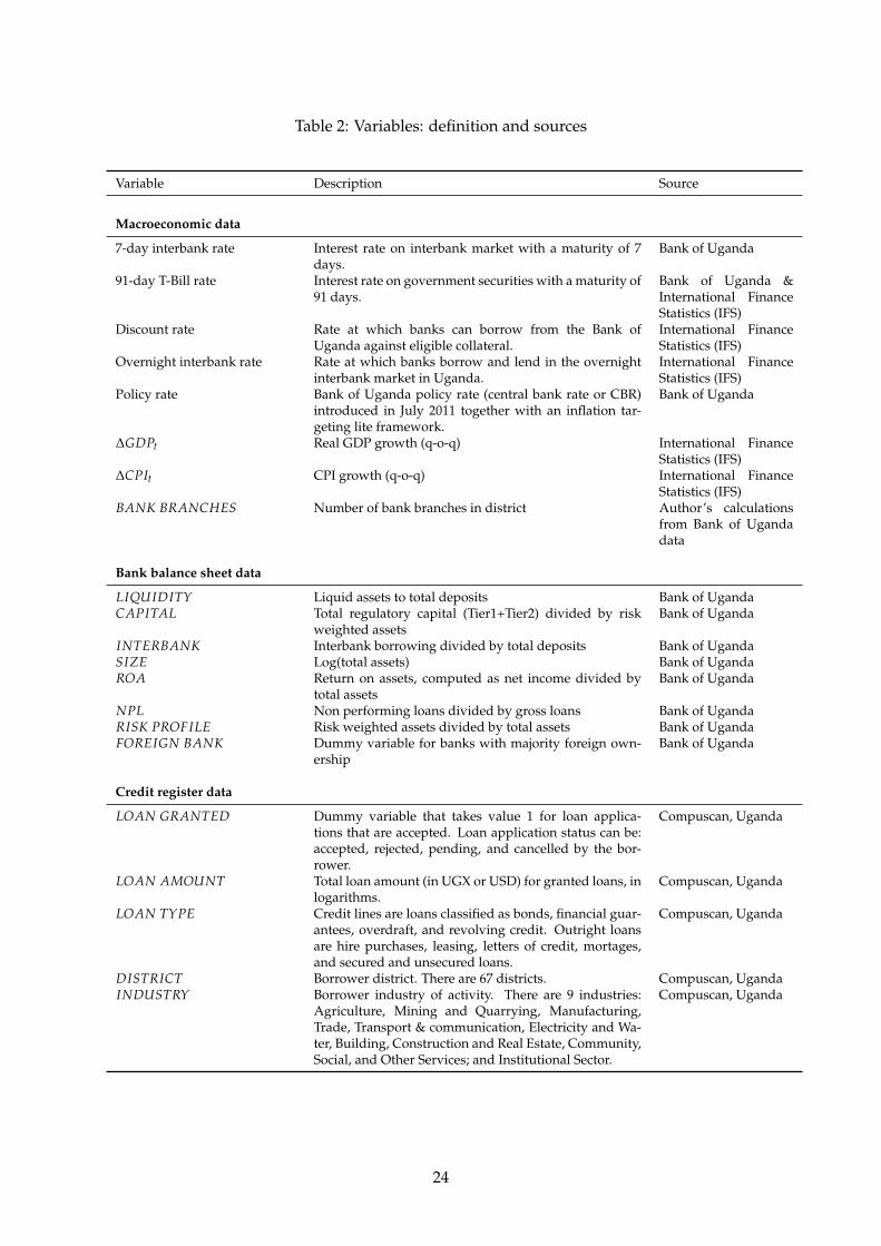
Table 2: Variables: definition and sources

Variable Description Source

Macroeconomic data

7-day interbank rate Interest rate on interbank market with a maturity of 7days.

Bank of Uganda

91-day T-Bill rate Interest rate on government securities with a maturity of91 days.

Bank of Uganda &International FinanceStatistics (IFS)

Discount rate Rate at which banks can borrow from the Bank ofUganda against eligible collateral.

International FinanceStatistics (IFS)

Overnight interbank rate Rate at which banks borrow and lend in the overnightinterbank market in Uganda.

International FinanceStatistics (IFS)

Policy rate Bank of Uganda policy rate (central bank rate or CBR)introduced in July 2011 together with an inflation tar-geting lite framework.

Bank of Uganda

∆GDPt Real GDP growth (q-o-q) International FinanceStatistics (IFS)

∆CPIt CPI growth (q-o-q) International FinanceStatistics (IFS)

BANK BRANCHES Number of bank branches in district Author’s calculationsfrom Bank of Ugandadata

Bank balance sheet data

LIQUIDITY Liquid assets to total deposits Bank of UgandaCAPITAL Total regulatory capital (Tier1+Tier2) divided by risk

weighted assetsBank of Uganda

INTERBANK Interbank borrowing divided by total deposits Bank of UgandaSIZE Log(total assets) Bank of UgandaROA Return on assets, computed as net income divided by

total assetsBank of Uganda

NPL Non performing loans divided by gross loans Bank of UgandaRISK PROFILE Risk weighted assets divided by total assets Bank of UgandaFOREIGN BANK Dummy variable for banks with majority foreign own-

ershipBank of Uganda

Credit register data

LOAN GRANTED Dummy variable that takes value 1 for loan applica-tions that are accepted. Loan application status can be:accepted, rejected, pending, and cancelled by the bor-rower.

Compuscan, Uganda

LOAN AMOUNT Total loan amount (in UGX or USD) for granted loans, inlogarithms.

Compuscan, Uganda

LOAN TYPE Credit lines are loans classified as bonds, financial guar-antees, overdraft, and revolving credit. Outright loansare hire purchases, leasing, letters of credit, mortages,and secured and unsecured loans.

Compuscan, Uganda

DISTRICT Borrower district. There are 67 districts. Compuscan, UgandaINDUSTRY Borrower industry of activity. There are 9 industries:

Agriculture, Mining and Quarrying, Manufacturing,Trade, Transport & communication, Electricity and Wa-ter, Building, Construction and Real Estate, Community,Social, and Other Services; and Institutional Sector.

Compuscan, Uganda

24

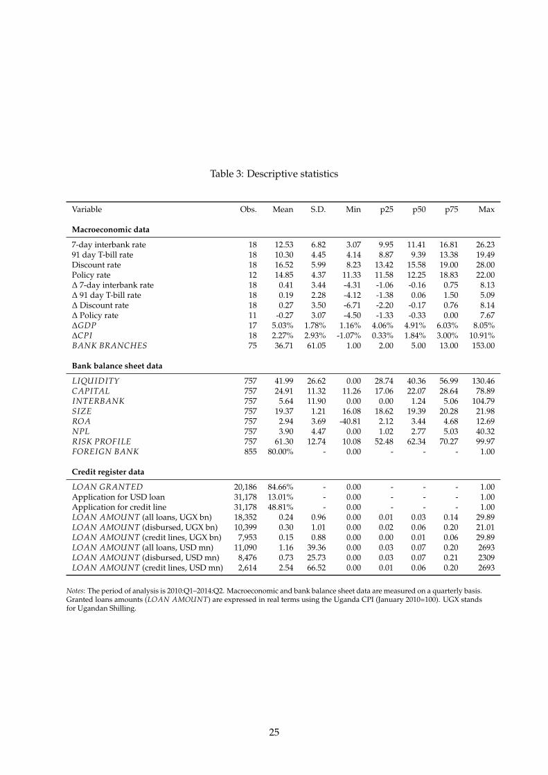
Table 3: Descriptive statistics

Variable Obs. Mean S.D. Min p25 p50 p75 Max

Macroeconomic data

7-day interbank rate 18 12.53 6.82 3.07 9.95 11.41 16.81 26.2391 day T-bill rate 18 10.30 4.45 4.14 8.87 9.39 13.38 19.49Discount rate 18 16.52 5.99 8.23 13.42 15.58 19.00 28.00Policy rate 12 14.85 4.37 11.33 11.58 12.25 18.83 22.00∆ 7-day interbank rate 18 0.41 3.44 -4.31 -1.06 -0.16 0.75 8.13∆ 91 day T-bill rate 18 0.19 2.28 -4.12 -1.38 0.06 1.50 5.09∆ Discount rate 18 0.27 3.50 -6.71 -2.20 -0.17 0.76 8.14∆ Policy rate 11 -0.27 3.07 -4.50 -1.33 -0.33 0.00 7.67∆GDP 17 5.03% 1.78% 1.16% 4.06% 4.91% 6.03% 8.05%∆CPI 18 2.27% 2.93% -1.07% 0.33% 1.84% 3.00% 10.91%BANK BRANCHES 75 36.71 61.05 1.00 2.00 5.00 13.00 153.00

Bank balance sheet data

LIQUIDITY 757 41.99 26.62 0.00 28.74 40.36 56.99 130.46CAPITAL 757 24.91 11.32 11.26 17.06 22.07 28.64 78.89INTERBANK 757 5.64 11.90 0.00 0.00 1.24 5.06 104.79SIZE 757 19.37 1.21 16.08 18.62 19.39 20.28 21.98ROA 757 2.94 3.69 -40.81 2.12 3.44 4.68 12.69NPL 757 3.90 4.47 0.00 1.02 2.77 5.03 40.32RISK PROFILE 757 61.30 12.74 10.08 52.48 62.34 70.27 99.97FOREIGN BANK 855 80.00% - 0.00 - - - 1.00

Credit register data

LOAN GRANTED 20,186 84.66% - 0.00 - - - 1.00Application for USD loan 31,178 13.01% - 0.00 - - - 1.00Application for credit line 31,178 48.81% - 0.00 - - - 1.00LOAN AMOUNT (all loans, UGX bn) 18,352 0.24 0.96 0.00 0.01 0.03 0.14 29.89LOAN AMOUNT (disbursed, UGX bn) 10,399 0.30 1.01 0.00 0.02 0.06 0.20 21.01LOAN AMOUNT (credit lines, UGX bn) 7,953 0.15 0.88 0.00 0.00 0.01 0.06 29.89LOAN AMOUNT (all loans, USD mn) 11,090 1.16 39.36 0.00 0.03 0.07 0.20 2693LOAN AMOUNT (disbursed, USD mn) 8,476 0.73 25.73 0.00 0.03 0.07 0.21 2309LOAN AMOUNT (credit lines, USD mn) 2,614 2.54 66.52 0.00 0.01 0.06 0.20 2693

Notes: The period of analysis is 2010:Q1–2014:Q2. Macroeconomic and bank balance sheet data are measured on a quarterly basis.Granted loans amounts (LOAN AMOUNT) are expressed in real terms using the Uganda CPI (January 2010=100). UGX standsfor Ugandan Shilling.

25

Table 4: Extensive margin of credit supply and monetary conditions – Baseline

Dep. Var.: LOAN GRANTEDijt (1) (2) (3) (4) (5)

∆IRt -0.0086*** -0.0057*** -0.0041*** -0.0134*(0.001) (0.001) (0.001) (0.007)

∆GDPt 0.7363*** 0.6161*** 4.3886***(0.186) (0.185) (0.780)

∆CPIt -0.0068*** -0.0050*** -0.0233***(0.001) (0.001) (0.005)

LIQUIDITYb,t−1 0.0032*** 0.0025** 0.0029***(0.001) (0.001) (0.001)

CAPITALb,t−1 0.0060*** 0.0088*** 0.0068***(0.002) (0.002) (0.001)

∆IRt × LIQUIDITYb,t−1 -0.0002** -0.0002**(0.000) (0.000)

∆IRt × CAPITALb,t−1 0.0009*** 0.0009***(0.000) (0.000)

∆GDPt × LIQUIDITYb,t−1 0.0125 0.0086(0.012) (0.013)

∆GDPt × CAPITALb,t−1 -0.2131*** -0.1730***(0.024) (0.022)

∆CPIt × LIQUIDITYb,t−1 0.0004*** 0.0004***(0.000) (0.000)

∆CPIt × CAPITALb,t−1 0.0000 -0.0001(0.000) (0.000)

Observations 20,118 20,118 20,118 20,118 20,118R2 0.486 0.488 0.493 0.497 0.499Firm FE Yes Yes Yes Yes YesBank FE Yes Yes Yes Yes YesQuarter FE No No No No Yes

Notes: The table reports regression results of a linear probability model in which the dependent variable is an indicator forsuccessful loan applications by firm i to bank b at time t. Standard errors, clustered at the district level, are reported in parentheses.* significant at 10%; ** significant at 5%; *** significant at 1%.

26

Table 5: Extensive margin of credit supply and monetary conditions – By loan currency

Dep. Var.: LOAN GRANTEDijt (1) (2) (3) (4) (5) (6)

UGX USD

∆IRt -0.0035*** -0.0048 -0.0105** -0.0481***(0.001) (0.008) (0.005) (0.014)

∆GDPt 0.6618*** 4.1019*** 0.5573*** 3.6421***(0.210) (1.325) (0.189) (0.834)

∆CPIt -0.0037** -0.0267*** -0.0111*** -0.0325***(0.002) (0.007) (0.004) (0.009)

LIQUIDITYb,t−1 0.0030** 0.0023 0.0027* 0.0063*** 0.0020 0.0020(0.001) (0.001) (0.001) (0.001) (0.002) (0.002)

CAPITALb,t−1 0.0070*** 0.0098*** 0.0078*** -0.0012 0.0050 0.0040(0.002) (0.002) (0.002) (0.004) (0.005) (0.005)

∆IRt × LIQUIDITYb,t−1 -0.0003** -0.0003* -0.0004 -0.0004(0.000) (0.000) (0.000) (0.000)

∆IRt × CAPITALb,t−1 0.0006** 0.0007*** 0.0029*** 0.0028**(0.000) (0.000) (0.001) (0.001)

∆GDPt × LIQUIDITYb,t−1 0.0230 0.0169 0.0344 0.0347(0.021) (0.020) (0.033) (0.028)

∆GDPt × CAPITALb,t−1 -0.2134*** -0.1786*** -0.2252*** -0.1559***(0.034) (0.032) (0.034) (0.049)

∆CPIt × LIQUIDITYb,t−1 0.0006*** 0.0006*** 0.0005*** 0.0005*(0.000) (0.000) (0.000) (0.000)

∆CPIt × CAPITALb,t−1 0.0001 -0.0000 -0.0000 -0.0003(0.000) (0.000) (0.001) (0.001)

Observations 17,485 17,485 17,485 2,633 2,633 2,633R2 0.513 0.517 0.519 0.517 0.535 0.546Firm FE Yes Yes Yes Yes Yes YesBank FE Yes Yes Yes Yes Yes YesQuarter FE No No Yes No No Yes

Notes: The table reports regression results of a linear probability model in which the dependent variable is an indicator forsuccessful loan applications by firm i to bank b at time (quarter) t. Standard errors, clustered at the district level, are reported inparentheses. * significant at 10%; ** significant at 5%; *** significant at 1%.

27

Tabl

e6:

Inte

nsiv

em

argi

nof

cred

itsu

pply

and

mon

etar

yco

ndit

ions

–Ba

selin

e,U

GX

loan

s

Dep

.Var

.:LO

AN

AM

OU

NT j

bt(1

)(2

)(3

)(4

)(5

)(6

)(7

)(8

)(9

)(1

0)(1

1)(1

2)

∆IR

t,t−

1-0

.008

5-0

.017

8-0

.008

2-0

.123

4**

(0.0

09)

(0.0

11)

(0.0

09)

(0.0

47)

∆IR

t,t−

1×

LIQ

UID

ITY b

,t−1

0.00

150.

0012

0.00

07(0

.001

)(0

.001

)(0

.002

)∆

IRt,t−

1×

CA

PIT

AL b

,t−1

0.00

30*

0.00

340.

0055

**(0

.002

)(0

.002

)(0

.002

)∆

IRt,t−

2-0

.014

9***

-0.0

115*

-0.0

056

-0.0

694*

*(0

.005

)(0

.006

)(0

.005

)(0

.027

)∆

IRt,t−

2×

LIQ

UID

ITY b

,t−1

0.00

03-0

.000

1-0

.000

4(0

.001

)(0

.001

)(0

.001

)∆

IRt,t−

2×

CA

PIT

AL b

,t−1

0.00

27**

*0.

0031

***

0.00

41**

*(0

.001

)(0

.001

)(0

.001

)∆

GD

P t11

.773

5***

10.7

979*

**32

.889

9***

10.5

212*

**10

.199

9***

25.0

984*

**(1

.886

)(1

.736

)(7

.899

)(2

.299

)(1

.942

)(8

.904

)∆

CP

I t-0

.003

00.

0068

-0.0

021

-0.0

028

0.00

70-0

.014

1(0

.013

)(0

.013

)(0

.043

)(0

.012

)(0

.012

)(0

.040

)L

IQU

IDIT

Y b,t−

10.

0147

***

0.02

30**

*0.

0251

***

0.02

59**

*0.

0145

***

0.02

35**

*0.

0264

***

0.02

80**

*(0

.004

)(0

.005

)(0

.006

)(0

.009

)(0

.004

)(0

.005

)(0

.006

)(0

.008

)C

AP

ITA

L b,t−

10.

0401

***

0.03

79**

0.03

140.

0148

0.03

99**

*0.

0280

0.01

980.

0008

(0.0

13)

(0.0

18)

(0.0

21)

(0.0

24)

(0.0

12)

(0.0

20)

(0.0

23)

(0.0

26)

∆G

DP t×

LIQ

UID

ITY b

,t−1

-0.3

833*

-0.3

914*

-0.5

088

-0.3

778*

-0.4

240*

*-0

.573

5**

(0.2

03)

(0.1

98)

(0.3

08)

(0.2

03)

(0.2

04)

(0.2

46)

∆G

DP t×

CA

PIT

AL b

,t−1

-0.3

509

-0.3

122

0.04

65-0

.015

20.

0747

0.53

80*

(0.2

81)

(0.2

83)

(0.2

77)

(0.3

27)

(0.3

53)

(0.2

75)

∆C

PI t×

LIQ

UID

ITY b

,t−1

-0.0

002

-0.0

011

-0.0

017

0.00

03-0

.000

5-0

.001

0(0

.001

)(0

.001

)(0

.001

)(0

.001

)(0

.001

)(0

.001

)∆

CP

I t×

CA

PIT

AL b

,t−1

0.00

060.

0009

0.00

060.

0003

0.00

050.

0005

(0.0

02)

(0.0

02)

(0.0

02)

(0.0

02)

(0.0

02)

(0.0

02)

Obs

erva

tion

s3,

624

3,62

43,

624

3,62

43,

624

3,62

43,

624

3,62

43,

624

3,62

43,

624

3,62

4R

20.

419

0.42

40.

430

0.43

20.

438

0.64

10.

420

0.42

40.

430

0.43

20.

438

0.64

2Ba

nkFE

Yes

Yes

Yes

Yes

Yes

Yes

Yes

Yes

Yes

Yes

Yes

Yes

Indu

stry

-dis

tric

tFE

Yes

Yes

Yes

Yes

Yes

Yes

Yes

Yes

Yes

Yes

Yes

Yes

Qua

rter

FEN

oN

oN

oN

oYe

sYe

sN

oN

oN

oN

oYe

sYe

sIn

dust

ry-d

istr

ict×

Qua

rter

FEN

oN

oN

oN

oN

oYe

sN

oN

oN

oN

oN

oYe

s

Not

es:T

heta

ble

repo

rts

regr

essi

onre

sult

sof

alin

earm

odel

inw

hich

the

depe

nden

tvar

iabl

eis

the

loan

amou

ntgr

ante

dto

borr

ower

sin

dist

rict

-spe

cific

indu

stry

jby

bank

bat

tim

e(q

uart

er)t

.Sta

ndar

der

rors

,clu

ster

edat

the

dist

rict

leve

l,ar

ere

port

edin

pare

nthe

ses.

*si

gnifi

cant

at10

%;*

*si

gnifi

cant

at5%

;***

sign

ifica

ntat

1%.

28

Tabl

e7:

Inte

nsiv

em

argi

nof

cred

itsu

pply

and

mon

etar

yco

ndit

ions

–Ba

selin

e,U

SDlo

ans

Dep

.Var

.:LO

AN

AM

OU

NT j

bt(1

)(2

)(3

)(4

)(5

)(6

)(7

)(8

)(9

)(1

0)(1

1)(1

2)

∆IR

t,t−

1-0

.004

5-0

.010

0-0

.016

2*-0

.114

1***

(0.0

10)

(0.0

09)

(0.0

09)

(0.0

34)

∆IR

t,t−

1×

LIQ

UID

ITY b

,t−1

0.00

03-0

.001

3-0

.001

8**

(0.0

01)

(0.0

01)

(0.0

01)

∆IR

t,t−

1×

CA

PIT

AL b

,t−1

0.00

44**

0.00

62**

*0.

0068

***

(0.0

02)

(0.0

02)

(0.0

02)

∆IR

t,t−

2-0

.010

2-0

.005

2-0

.007

8**

-0.0

590*

*(0

.006

)(0

.004

)(0

.003

)(0

.024

)∆

IRt,t−

2×

LIQ

UID

ITY b

,t−1

0.00

08**

-0.0

003

-0.0

009*

**(0

.000

)(0

.000

)(0

.000

)∆

IRt,t−

2×

CA

PIT

AL b

,t−1

0.00

100.

0022

**0.

0019

*(0

.001

)(0

.001

)(0

.001

)∆

GD

P t12

.688

1**

11.8

449*

*13

.445

512

.086

7**

10.9

195*

*7.

4681

(4.7

59)

(4.8

88)

(10.

053)

(4.3

92)

(4.5

51)

(8.5

56)

∆C

PI t

-0.0

141

-0.0

080

0.10

71-0

.015

0-0

.009

90.

0933

(0.0

12)

(0.0

15)

(0.0

84)

(0.0

15)

(0.0

17)

(0.0

80)

LIQ

UID

ITY b

,t−1

0.01

30**

*0.

0055

-0.0

002

-0.0

010

0.01

29**

*0.

0048

*0.

0016

0.00

10(0

.004

)(0

.003

)(0

.006

)(0

.012

)(0

.004

)(0

.002

)(0

.004

)(0

.012

)C

AP

ITA

L b,t−

1-0

.036

8***

-0.0

129

-0.0

319*

*-0

.027

5-0

.036

2***

-0.0

149

-0.0

376*

**-0

.034

3*(0

.011

)(0

.014

)(0

.013

)(0

.019

)(0

.010

)(0

.013

)(0

.013

)(0

.019

)∆

GD

P t×

LIQ

UID

ITY b

,t−1

0.15

320.

0860

0.14

480.

2269

*0.

0472

0.05

80(0

.104

)(0

.096

)(0

.230

)(0

.116

)(0

.082

)(0

.224

)∆

GD

P t×

CA

PIT

AL b

,t−1

-0.3

980*

*-0

.244

4*-0

.525

1***

-0.2

801*

0.01

97-0

.241

8*(0

.184

)(0

.133

)(0

.143

)(0

.159

)(0

.100

)(0

.122

)∆

CP

I t×

LIQ

UID

ITY b

,t−1

0.00

27**

*0.

0056

***

0.00

59**

*0.

0023

***

0.00

52**

*0.

0057

***

(0.0

01)

(0.0

01)

(0.0

01)

(0.0

01)

(0.0

01)

(0.0

01)

∆C

PI t×

CA

PIT

AL b

,t−1

-0.0

109*

*-0

.014

3***

-0.0

141*

**-0

.009

6**

-0.0

130*

**-0

.012

1***

(0.0

04)

(0.0

04)

(0.0

04)

(0.0

04)

(0.0

04)

(0.0

03)

Obs

erva

tion

s1,

032

1,03

21,

032

1,03

21,

032

1,03

21,

032

1,03

21,

032

1,03

21,

032

1,03

2R

20.

234

0.24

00.

243

0.24

60.

267

0.42

70.

235

0.24

00.

243

0.24

60.

266

0.42

6Ba

nkFE

Yes

Yes

Yes

Yes

Yes

Yes

Yes

Yes

Yes

Yes

Yes

Yes

Indu

stry

-dis

tric

tFE

Yes

Yes

Yes

Yes

Yes

Yes

Yes

Yes

Yes

Yes

Yes

Yes

Qua

rter

FEN

oN

oN

oN

oYe

sYe

sN

oN

oN

oN

oYe

sYe

sIn

dust

ry-d

istr

ict×

Qua

rter

FEN

oN

oN

oN

oN

oYe

sN

oN

oN

oN

oN

oYe

s

Not

es:T

heta

ble

repo

rts

regr

essi

onre

sult

sof

alin

earm

odel

inw

hich

the

depe

nden

tvar

iabl

eis

the

loan

amou

ntgr

ante

dto

borr

ower

sin

dist

rict

-spe

cific

indu

stry

jby

bank

bat

tim

e(q

uart

er)t

.Sta

ndar

der

rors

,clu

ster

edat

the

dist

rict

leve

l,ar

ere

port

edin

pare

nthe

ses.

*si

gnifi

cant

at10

%;*

*si

gnifi

cant

at5%

;***

sign

ifica

ntat

1%.

29

Table 8: Extensive margin of credit supply and monetary conditions – Additional tests

Dep. Var.: LOAN GRANTEDijt (1) (2) (3) (4) (5)Bank vars By loan type: By ownership:

Credit lines Outright loans Foreign Domestic

∆IRt -0.0126* -0.0023 -0.0297** -0.0089 0.0020(0.007) (0.006) (0.014) (0.008) (0.008)

∆GDPt 4.0973*** 4.9694*** 4.1408*** 4.8050*** -0.1220(0.731) (0.918) (1.109) (0.956) (2.016)

∆CPIt -0.0235*** -0.0278*** -0.0307*** -0.0257*** 0.0037(0.005) (0.008) (0.010) (0.006) (0.013)

LIQUIDITYb,t−1 0.0018** 0.0011 0.0028** 0.0023** -0.0003(0.001) (0.001) (0.001) (0.001) (0.000)

CAPITALb,t−1 0.0092*** 0.0078*** 0.0080*** 0.0117*** 0.0010(0.002) (0.002) (0.002) (0.002) (0.002)

∆IRt × LIQUIDITYb,t−1 -0.0002** -0.0002* -0.0005** -0.0002* 0.0000(0.000) (0.000) (0.000) (0.000) (0.000)

∆IRt × CAPITALb,t−1 0.0010*** 0.0005** 0.0021*** 0.0006* -0.0001(0.000) (0.000) (0.001) (0.000) (0.000)

∆GDPt × LIQUIDITYb,t−1 0.0192 -0.0056 0.0467* 0.0095 0.0235(0.014) (0.020) (0.026) (0.015) (0.028)

∆GDPt × CAPITALb,t−1 -0.2163*** -0.2083*** -0.2479*** -0.2345*** -0.0304(0.023) (0.025) (0.047) (0.029) (0.119)

∆CPIt × LIQUIDITYb,t−1 0.0005*** 0.0007*** 0.0001 0.0006*** 0.0001(0.000) (0.000) (0.000) (0.000) (0.000)

∆CPIt × CAPITALb,t−1 -0.0000 -0.0002 0.0008* -0.0002 -0.0004(0.000) (0.000) (0.000) (0.000) (0.001)

SIZE -0.0215(0.016)

ROA 0.0046*(0.003)

NPL 0.0136***(0.003)

BANK BRANCHES 0.0001(0.000)

Observations 20,118 10,333 9,785 14,859 5,259R2 0.499 0.474 0.652 0.477 0.717Firm FE Yes Yes Yes Yes YesBank FE Yes Yes Yes Yes YesQuarter FE No No No No No

Notes: The table reports regression results of a linear probability model in which the dependent variable is an indicator forsuccessful loan applications by firm i to bank b at time (quarter) t. Standard errors, clustered at the district level, are reported inparentheses. * significant at 10%; ** significant at 5%; *** significant at 1%.

30

Tabl

e9:

Inte

nsiv

em

argi

nof

cred

itsu

pply

and

mon

etar

yco

ndit

ions

–A

lter

nati

veid

enti

ficat

ion

stra

tegy

Dep

.Var

.:(1

)(2

)(3

)(4

)(5

)(6

)(7

)(8

)

∆LO

AN

AM

OU

NT

Unw

eigh

ted

Wei

ghte

d

INT

ER

BA

NK

-0.2

87**

*-0

.286

***

-0.4

94**

*-0

.677

***

-0.2

76**

*-0

.256

***

-0.4

88**

*-0

.759

***

(0.0

49)

(0.0

74)

(0.1

04)

(0.1

36)

(0.0

42)

(0.0

66)

(0.0

89)

(0.1

62)

FOR

EIG

NB

AN

K2.

958*

**2.

271*

**3.

064*

**2.

607*

**3.

203*

**2.

409*

**3.

197*

**2.

672*

**(0

.529

)(0

.517

)(0

.480

)(0

.360

)(0

.382

)(0

.535

)(0

.340

)(0

.296

)S

IZE

0.99

5***

0.91

1**

1.03

4***

1.24

3***

1.05

5***

0.83

0**

1.06

7***

1.19

8***

(0.2

26)

(0.3

30)

(0.2

27)

(0.2

36)

(0.2

02)

(0.3

55)

(0.2

04)

(0.2

31)

RIS

KP

RO

FIL

E0.

098*

**0.

046*

0.11

5***

0.07

9***

0.10

9***

0.04

60.

119*

**0.

076*

**(0

.030

)(0

.022

)(0

.028

)(0

.019

)(0

.022

)(0

.027

)(0

.021

)(0

.020

)N

PL

0.12

40.

163*

*0.

138

0.22

6***

0.14

3*0.

183*

**0.

155*

*0.

227*

**(0

.087

)(0

.058

)(0

.083

)(0

.053

)(0

.074

)(0

.044

)(0

.067

)(0

.064

)L

IQU

IDIT

Y0.

056*

*0.

052*

**0.

062*

**0.

051*

**(0

.020

)(0

.015

)(0

.017

)(0

.014

)C

AP

ITA

L0.

022

0.02

5**

0.01

70.

021*

(0.0

15)

(0.0

09)

(0.0

18)

(0.0

10)

LIQ

UID

ITY×

INT

ER

BA

NK

0.00

8**

0.00

8**

(0.0

03)

(0.0

03)

CA

PIT

AL×

INT

ER

BA

NK

0.02

3***

0.02

9***

(0.0

07)

(0.0

09)

Obs

erva

tion

s24

624

624

624

624

624

624

624

6R

20.

406

0.39

50.

408

0.40

70.

441

0.41

40.

446

0.43

6In

dust

ry-d

istr

ictF

EYe

sYe

sYe

sYe

sYe

sYe

sYe

sYe

s

Not

es:

The

tabl

ere

port

sre

gres

sion

resu

lts

ofa

linea

rm

odel

inw

hich

the

depe

nden

tva

riab

leis

the

log

diff

eren

ceof

tota

lloa

nvo

lum

esgr

ante

dto

dist

rict

-spe

cific

indu

stry

jby

bank

bbe

twee

nth

e(2

010:

m1-

2011

:m6)

peri

odan

dth

e(2

011:

m7-

2012

:m12

)per

iod.

The

peri

ods

are

sepa

rate

dby

the

intr

oduc

tion

ofth

eIT

-lit

em

onet

ary

polic

yfr

amew

ork

(201

1:m

7).A

llba

nk-l

evel

vari

able

sar

em

easu

red

asof

2011

:Q2

(pre

-IT

lite)

.In

colu

mns

5-8

the

obse

rvat

ions

are

wei

ghte

dby

the

inve

rse

ofth

enu

mbe

rof

tim

esea

chba

nkap

pear

sin

the

data

set(

ina

pair

wit

ha

borr

owin

gin

dust

ry).

The

wei

ghti

ngsc

hem

eco

ntro

lsfo

rth

efa

ctth

atth

eba

lanc

esh

eets

ofve

ryac

tive

bank

s(t

hatl

end

tom

any

indu

stri

es)a

ppea

rin

the

data

setm

ore

freq

uent

lyth

anth

ose

ofle

ssac

tive

bank

s.R

obus

tsta

ndar

der

rors

that

are

clus

tere

dat

the

dist

rict

-spe

cific

indu

stry

leve

lare

repo

rted

inpa

rent

hese

s.*

sign

ifica

ntat

10%

;**

sign

ifica

ntat

5%;*

**si

gnifi

cant

at1%

.

31