The Balassa-Samuelson Effect Reversed: New Evidence from OECD Countries Matthias Gubler and Christoph Sax

SNB Working Papers 1/2017

DISCLAIMER The views expressed in this paper are those of the author(s) and do not necessarily represent those of the Swiss National Bank. Working Papers describe research in progress. Their aim is to elicit comments and to further debate. COPYRIGHT© The Swiss National Bank (SNB) respects all third-party rights, in particular rights relating to works protected by copyright (infor-mation or data, wordings and depictions, to the extent that these are of an individual character). SNB publications containing a reference to a copyright (© Swiss National Bank/SNB, Zurich/year, or similar) may, under copyright law, only be used (reproduced, used via the internet, etc.) for non-commercial purposes and provided that the source is menti-oned. Their use for commercial purposes is only permitted with the prior express consent of the SNB. General information and data published without reference to a copyright may be used without mentioning the source. To the extent that the information and data clearly derive from outside sources, the users of such information and data are obliged to respect any existing copyrights and to obtain the right of use from the relevant outside source themselves. LIMITATION OF LIABILITY The SNB accepts no responsibility for any information it provides. Under no circumstances will it accept any liability for losses or damage which may result from the use of such information. This limitation of liability applies, in particular, to the topicality, accu−racy, validity and availability of the information. ISSN 1660-7716 (printed version) ISSN 1660-7724 (online version) © 2017 by Swiss National Bank, Börsenstrasse 15, P.O. Box, CH-8022 Zurich

Legal Issues

3

The Balassa-Samuelson Effect Reversed:

New Evidence from OECD Countries∗

Matthias Gubler†

Swiss National Bank

Christoph Sax‡

University of Basel

December 2016

Abstract

This paper explores the robustness of the Balassa-Samuelson (BS) hypothesis. We analyze an

OECD country panel from 1970 to 2008 and compare three data sets on sectoral productivity,

including newly constructed data on total factor productivity. Overall, our within- and

between-dimension estimation results do not support the BS hypothesis. Over the last

two decades, we find a robust negative relationship between productivity in the tradable

sector and the real exchange rate, even after including the terms of trade to control for the

deviations from the law of one price. Earlier supportive findings depend on the choice of

the data set and the model specification.

JEL Classifications: F14, F31, F41

Keywords: Real Exchange Rate, Balassa-Samuelson Hypothesis, Panel Data Estimation,

Terms of Trade

∗Without reservation, we would like to thank Sylvia Kaufmann, Markus Ludwig, Christian Rutzer, LindaWalter, Rolf Weder, an anonymous referee and the seminar participants at the University of Basel for theirextensive comments and suggestions, as well as the OECD for kindly sharing two essential data sets on sectoralproductivity. Hermione Miller-Moser provided excellent editorial assistance. Matthias Gubler is indebted to PeterKugler for his help and supervision. Christoph Sax acknowledges support from the WWZ Forum Foundation.The views, opinions, findings, and conclusions or recommendations expressed in this paper are strictly thoseof the author(s). They do not necessarily reflect the views of the Swiss National Bank. The SNB takes noresponsibility for any errors or omissions in, or for the correctness of, the information contained in this paper.

†Contact Address: Swiss National Bank, Börsenstrasse 15, P.O. Box, 8022 Zürich, Switzerland. Email:matthias.gubler@snb.ch. Phone: +41 58 631 32 46

‡Contact Address: University of Basel, Peter Merian-Weg 6, 4002 Basel, Switzerland.

4

1 Introduction

The Balassa-Samuelson (BS) hypothesis—stated by both Balassa (1964) and Samuelson (1964),

with a research precedent in the work of Harrod (1933)—is one of the most widespread expla-

nations for structural deviations from purchasing power parity (PPP).1

According to the BS hypothesis, differences in the productivity differential between the

non-tradable and the tradable sector lead to differences in price levels between countries when

converted to the same currency. The hypothesis assumes that the law of one price for tradable

goods holds.Ceteris paribus, a productivity increase in tradables raises factor prices, i.e., wages,

which in turn leads to higher prices of non-tradables and thus to an appreciation of the real

exchange rate. In contrast, when the relative productivity of non-tradables increases, marginal

cost cuts result in a lower price level.

The empirical evaluation of the BS hypothesis has gained a great deal of attention. As

argued in a survey by Tica and Družić (2006), the major share of the evidence supports the BS

model, but the strength of the results depends on the nature of the tests and set of countries

analyzed.

There are several studies based on a disaggregation of the tradable and non-tradable sector

that find empirical support for the BS hypothesis (see, e.g., Calderón, 2004; Choudhri and Khan,

2005; Ricci et al., 2013 or Berka et al., 2014). In particular, since sector-specific data for OECD

countries on total factor productivity (TFP) have become available, various studies have tested

and confirmed the BS hypothesis using panel data (De Gregorio et al., 1994; De Gregorio and

Wolf, 1994; Chinn and Johnston, 1996; MacDonald and Ricci, 2007). All these studies are based

on the discontinued International Sectoral Database (ISDB) provided by the OECD.

This paper applies a panel cointegration model to estimate the long-run relationship between

the real exchange rate and key explanatory variables, focusing on the effect of the TFP differential

between tradables and non-tradables. We use a novel OECD data set (PDBi) with sector-specific

TFP data from 1984 to 2008 to eliminate some of the shortcomings of the ISDB.

With this new data set, our estimations cannot confirm the findings of previous research1Rogoff (1996) shows that the speed of adjustment of real exchange rates is too slow to be in line with the

PPP theory. Recent studies challenge this finding and stress the importance of nonlinear adjustments (Taylor,2003) or dynamic aggregation bias (Imbs et al., 2005). Altogether, the empirical evidence for PPP is mixed (forreviews, see Froot and Rogoff, 1996; Taylor, 2003 or Gengenbach et al., 2009).

2

5

based on the ISDB.2 In fact, the results point to a negative relationship between tradable

productivity and the real exchange rate. In other words, over the last two decades, an increase

in the productivity of tradables has given rise to a depreciation of the real exchange rate. This

finding is the opposite of what is claimed by the BS hypothesis. We can confirm this result

when TFP is replaced by labor productivity (LP) using the OECD Structural Analysis (STAN)

data set, which covers more countries and a longer time period, from 1970 to 2008. A rigorous

analysis of the tradable sector reveals that this reversal is robust for the last two decades against

the choice of the productivity measure, the choice of the country sample, the precise start of

the sample period, the exact model specification, and the inclusion of additional explanatory

variables.

While Fazio et al. (2007) also find a statistically significant negative relationship between

the labor productivity of tradables and the real exchange rate for OECD countries, our analysis

also relies on sector-specific TFP, which is the preferred measure for productivity as noted by

De Gregorio and Wolf (1994).3

Based on these findings, we conclude that the theoretical framework leading to the Balassa-

Samuelson hypothesis needs to be modified to be in line with the empirical data. The literature

has proposed deviations from the law of one price, such as a home bias in consumption preferences

as a possible modification. Benigno and Thoenissen (2003) develop a new open economy model

in which a TFP shock in the tradable sector lowers the price of its goods relative to that abroad.

This may offset the increase of the relative price of non-traded goods.4 MacDonald and Ricci

(2007) and Choudhri and Schembri, 2010 provide similar explanations.5 However, we use the

terms of trade to control for the impact of movements in exports relative to import prices on

the real exchange rate. The inclusion of the terms of trade does not change the significant

negative relationship between the productivity of tradables and the real exchange rate. This

result suggests that a productivity increase in the tradable sector can lead to a decrease in the2However, we are indeed able to replicate the results in favor of the BS hypothesis with data from the ISDB.3Ricci et al. (2013) also find a negative relationship between the LP of tradables and the real exchange rate

for advanced countries, though this is not statistically significant.4There are also empirical contributions to the literature that find deviations from the law of one price (see,

e.g., Engel (1999)).5In the small economy model developed by Devereux (1999), the real exchange rate depreciates because

endogenous productivity gains in the service sector lead to a fall in traded goods prices that offsets the BS effect.However, because we exclude the distribution subsector due to classification difficulties (MacDonald and Ricci,2005), this seems not to be the main mechanism that explains the potentially negative relationship between risingproductivity in the tradable sector and the real exchange rate in our study. Moreover, Bordo et al. (2014) showthat the impact of productivity on the real exchange rate can vary over time due to changes in trade costs.

3

6

relative price of non-traded goods. Gubler and Sax (2014) provide a static general-equilibrium

framework with skill-based technological change (SBTC), in which higher productivity in the

tradable sector can lower wages, which in turn leads to lower prices of non-tradables and thus

to a depreciation of the real exchange rate.

On the other hand, the connection between non-tradable productivity and the real exchange

rate is not robust. Our robustness tests reveal that severe outlier dependency exists for the

traditional Balassa-Samuelson finding regarding non-tradables. In particular, Japanese labor

productivity in the non-tradable sector strongly weakens the estimated BS effect. For the time

period from 1970 to 1992, the coefficient even significantly changes its sign once Japan is included.

Finally, with the exception of the terms of trade, our estimation results indicate that the

explanatory power of further control variables discussed in the literature is weak or not robust.

The remainder of this paper is organized as follows. Section 2 presents the data. We outline

the methodology in Section 3 and show the results in Section 4. Section 5 concludes.

2 Data

The data for the 18 major OECD countries included in our data set stem from different data

sets of the IMF, OECD, World Bank and the Penn World Tables. Depending on the estimation,

the country sample has to be reduced because we aim to replicate the results of MacDonald

and Ricci (2007) or because not all data are available.6 A detailed description of all variables is

given in Table 1 and in Appendix A.2.

To test the BS hypothesis, we condition the real exchange rate on productivity measures

for both the tradable and the non-tradable sector as well as on control variables. The choice

of the dependent variable is discussed in Section 2.1. Due to its importance and complexity,

the productivity data are separately examined in Section 2.2. All other exogenous variables are

discussed in Section 2.3. The time series properties of the variables are assessed in Section 2.4.

2.1 Dependent Variable: Real Exchange Rate

We use the logarithm of the unweighted real exchange rate (RER) as the dependent variable

in our estimation equations. In principle, the real exchange rate can only be computed towards6All country samples featured in our estimations are presented in Appendix A.1.

4

7

Table 1: Description and Construction of the Variables

Abbr. Name Definition Source

RER Real Exchange Rate log(CPI / Nominal Exchange Rate to USD) IMF, IFS

TFP.TPDBi TFP of Tradables Solow Residual OECD, PDBiTFP.NTPDBi TFP of Non-Tradables Solow Residual OECD, PDBi

LP.TSTAN LP of Tradables log(Value Added / Hours-Worked) OECD, STANLP.NT STAN LP of Non-Tradables log(Value Added / Hours-Worked) OECD, STAN

TFP.T ISDB TFP of Tradables Solow Residual OECD, ISDBTFP.NT ISDB TFP of Non-Tradables Solow Residual OECD, ISDBLP.T ISDB LP of Tradables log(Value Added / Hours-Worked) OECD, ISDBLP.NT ISDB LP of Non-Tradables log(Value Added / Hours-Worked) OECD, ISDB

CA Current Account as % of GDP OECD, EODPOP Population Growth ∆ log(Population) PWTGDP Real GDP per Capita log(Real GDP per capita) PWTGOV Government Spending as % of GDP OECD, EONFA Net Foreign Assets as % of GDP WB, WDIRI Long-Term Real Int. Rate Gov. bond yield long term - CPI IMF, IFSTOT Terms of Trade log(Export-Prices / Import-Prices) OECD, EO

a reference currency; in our case, the US dollar. However, since we use the time-fixed effects

throughout our analysis, the choice of the reference currency does not impact the results. For

example, switching from the US dollar to the euro as a reference currency changes only the

time-fixed effects, leaving the other coefficients unchanged. Proceeding this way allows us to

keep all available countries in the sample.

An extensive body of the empirical literature uses effective real exchange rates (see, e.g., De

Gregorio and Wolf, 1994; Calderón, 2004 or Ricci et al., 2013) that are weighted by the share

of exports. Effective real exchange rates have the advantage that there is no need to specify a

reference country. While effective real exchange rates are a useful measure for competitiveness,

the share of exports seems not only irrelevant in our context but also misleading. If, for example,

a country changes its export destinations to countries with a weaker real exchange rate, effective

real exchange rates would indicate a real appreciation, while, in fact, the country still has the

same relative price level towards all countries.7

2.2 Productivity Data

We use data on sectoral productivity from three data sets provided by the OECD. The first

is a new data set on sectoral total factor productivity (TFP) computed by the OECD, called7Nonetheless, our main results are robust against the inclusion of the effective real exchange rate (source:

OECD Economic Outlook, competitiveness indicator) instead of the unweighted real exchange rate, RER.

5

8

PDBi. PDBi extends the older PDB by providing sector-specific TFP numbers. The data set

contains annual sector-specific TFP numbers and covers the time period from 1984 to 2008.

Sectoral TFP is calculated as Solow residuals with the same method for all countries, using

sectoral data on production, employment, capital stock and the labor share of income. Capital

stocks are estimated by applying the permanent inventory method, where streams of investments

are added, and a certain fraction of depreciation is subtracted each year (for more details, see

Arnaud et al., 2011).

A second data set, STAN, includes yearly data on sectoral production and employment—and

thus on labor productivity—but not on TFP. As the only data set, STAN covers a long time

range, from 1970 to 2008, for many OECD countries.

To compare our findings with the existing studies, particularly with the results of MacDonald

and Ricci (2007), sectoral productivity data from the discontinued ISDB have been used as well.

This old data set contains annual values on labor and total factor productivity—in principle

from 1970 to 1997—but was discontinued before 1997 for most countries.

STAN and PDBi data are improvements to the ISDB. In the old data set, output, employment

and capital stocks were based on data from an old system of national accounts, SNA68. For

social services, these changes in the measurement of output may have been especially important

because the estimates of the real value added growth for the public sector in the ISDB have

simply been based on labor inputs such that the estimates of productivity had very limited

meaning. Moreover, in the ISDB, volumes were calculated using constant prices instead of

chained linking. Finally, capital stock estimates may have been calculated differently and in a

non-standardized way in the ISDB.8

The classification of the subsectors into tradable and non-tradable is done according to

the following scheme: agriculture, manufacturing, and transport, storage and communications

are classified as tradables; utilities (energy, gas and water), construction, and social services

(community, social, personal services) are non-tradables. Our division of the subsectors into

tradable or non-tradable sectors follows De Gregorio and Wolf (1994), who defined a subsector

as tradable if its share of exports in the total production exceeds 10% and as non-tradable8While these are very general observations about the evolution of the system of national accounts, it would

be desirable if international organizations could provide more information about the changes over time. As inthe present case, this would significantly facilitate the task of replicating the earlier results.

6

9

otherwise.9 While no division has become standard in the field (Tica and Družić, 2006), studies

based on data from OECD countries usually refer to the division proposed by De Gregorio and

Wolf (1994) (see, e.g., Chinn and Johnston, 1996; MacDonald and Ricci, 2007). Like MacDonald

and Ricci (2007), we exclude distribution, mining and financial subsectors due to classification

difficulties (MacDonald and Ricci, 2005) or data availability.

The tradable and non-tradable sectors, when classified this way, are roughly equal in terms

of the value added. Each sector comprises 50% of the total value added that was produced by

these six subsectors. Within the tradable sector, manufacturing is by far the largest subsector,

representing 64% of the value added, whereas agriculture and transport as well as storage and

communications amount to 11% and 24%, respectively. Among the non-tradables, social services

(70%) outweigh construction (20%) and utilities (9%). Figure 2 in Appendix A displays the data

availability in each of the three data sets.

Table 2 shows the correlations between the three data sets. The LP and TFP values from the

ISDB are similar to the two newer data sets only in the tradable subsectors. In the non-tradable

sectors, the correlations are lower (construction and utilities) or virtually non-existent (social

services). To a lesser extent, this is also true for employment and value added. Possible reasons

for these divergences have been discussed earlier in this section. On the other hand, the data

from the PDBi on TFP are highly correlated with labor productivity from the STAN data set.

These correlations are present in all subsectors, although the values are somewhat lower in the

non-tradable subsectors.

We consider TFP to be the preferred measure for productivity. As noted by De Gregorio

and Wolf (1994), the average labor productivity increases much more quickly during economic

downturns; hence, it is not a reliable indicator of sustainable productivity growth, which can

affect the economy in the medium or long term. Nevertheless, there are some advantages of LP,

and we will use the measure to check the robustness of our TFP results.10

9Adjustments of the threshold value to 5% and 20% leave the division virtually unchanged (De Gregorio andWolf, 1994).

10The advantages are summarized by Canzoneri et al. (1999): First, the labor productivity data are availablefor more countries and over a longer time period than the TFP numbers. Second, the calculation of LP figuresdoes not require an estimation of the capital stock and the income share of labor, with both estimations likely tobe imprecise. Third, the BS hypothesis holds for more technologies than the Cobb-Douglas production function,which is generally employed to determine TFP.

7

10

Table 2: Median Correlations across Subsectors

AGR IND TSC EGW CST SOC

PDBi (TFP), STAN (LP) 0.95 0.97 0.92 0.95 0.93 0.84ISDB (TFP), STAN (LP) 0.90 0.91 0.93 0.75 0.76 0.28ISDB (TFP), ISDB (LP) 0.99 0.98 0.98 0.96 0.94 0.97ISDB (LP), STAN (LP) 0.90 0.88 0.88 0.72 0.77 0.27ISDB (EMP), STAN (EMP) 0.91 0.98 0.91 0.89 0.99 0.45ISDB (VA), STAN (VA) 0.91 0.95 0.89 0.72 0.93 0.45

Notes: The table contains median correlation coefficients between the variables in the three data sets for all six subsectors.The values are based on all countries for which a correlation coefficient can be calculated, including AGR: agriculture; IND:manufacturing; TSC: transport, storage and communications; EGW: energy, gas and water; CST: construction; and SOC:community, social, personal services. The first three rows show the median correlations between TFP from the PDBi or theISDB and LP from the STAN data set or the ISDB. The median correlations between the LP from the STAN data set andthe ISDB are reported in the fourth row. The last two rows contain the median correlation values between the EMP fromthe ISBD and the STAN data set and between VA from the same sources. Due to the very low number of time-overlappingobservations, no comparison between the PDBi and the ISDB is presented.

2.3 Control Variables

Along with the data on sectoral productivity, we take into account further potential determinants

of the long-run real exchange rate, which have been proposed in the literature. As described by

De Gregorio and Wolf (1994) or Sax and Weder (2009), among others, an improvement in the

terms of trade (TOT ) allows a country to raise its imports for a given number of factor inputs

in the export sector. For example, a change in consumer preferences may shift global demand

towards a specific country’s export goods. As a result, the good’s global price increases and,

hence, the country’s real exchange rate appreciates. Moreover, according to the model developed

by Benigno and Thoenissen (2003), changes in productivity in the tradable sector of a country

affect the real exchange rate through a change in the relative price of non-traded goods and an

adjustment of the terms of trade due to the home bias in consumption preferences. The latter

contradicts the BS hypothesis that assumes that the law of one price for tradable goods holds.

The terms of trade (TOT ) therefore also capture deviations from the law of one price.

Several authors note the importance of demand-side factors for the determination of the

long-run real exchange rate. Therefore, we consider the government spending share (GOV ), net

foreign assets relative to GDP (NFA), the current account relative to GDP (CA) and real GDP

per capita (GDP ) as control variables.

De Gregorio and Wolf (1994) show theoretically that an increase in government spending

causes the equilibrium real exchange rate to appreciate if capital mobility across countries is

restricted. This increase affects the relative price of tradable and non-tradable goods negatively

8

11

because government spending tends to fall more heavily on non-tradables. Hence, government

spending is widely used as an additional explanatory variable (see, e.g., Chinn and Johnston,

1996; Sax and Weder, 2009 or Ricci et al., 2013).

Private demand may affect the real exchange rate as well. It is likely that a higher income is

associated with a higher demand for non-tradables. The associated rise in the relative price of

non-tradables gives rise to a higher overall price level (De Gregorio and Wolf, 1994). Furthermore,

trade deficits or surpluses could affect the demand for non-tradables by increasing or decreasing

the amount of tradables that are available for consumption. As a permanent trade deficit can

only be sustained in the presence of net foreign assets, several authors have emphasized the

importance either of the net foreign assets or the current account deficit for the determination

of the real exchange rate (Krugman, 1990; Lane and Milesi-Ferretti, 2004; Ricci et al., 2013).

Finally, two other macroeconomic variables, the real interest rate (RI ) and the population

growth rate (DPOP), are taken into account. Their importance for the determination of RER

has been discussed in theoretical and empirical contributions to the literature. According to the

theoretical model provided by Stein and Allen (1997), a higher real interest rate is associated

with an appreciated long-run real exchange rate because of portfolio adjustments and capital

inflows. Rose et al. (2009) show in an overlapping generation model that a country experiencing

a decline in its fertility rate will also experience real exchange rate depreciation.

2.4 Assessing the Time Series Properties of the Variables

The panel unit root tests proposed by Levin et al. (2002) (LLC) and Im et al. (2003) (IPS)

have been conducted for all variables (Table 3). To obtain reliable results, the test statistics are

based on all available information for both time and cross-sectional dimensions.

As described in Section 2.1, we use time-specific dummy variables in all estimations. To be

consistent in assessing the times series properties, the real exchange rate is calculated for every

year towards the annual average of the sample (denoted RER.AV G). Again, the reference

currency is therefore irrelevant.

Overall, we find strong evidence for non-stationary behavior for all variables, with the ex-

ception of the population growth rate, DPOP . Because DPOP is the first difference of the

logarithm of the population, this result is not surprising. The total factor productivity in the

9

12

Table 3: IPS and LLC Panel Unit Root Test Results

Det. IPS LLC No. of Time Obs.Trend Countries Period

CA 0.933 0.994 18 1970-2008 587DPOP −4.269∗∗∗ −2.837∗∗∗ 18 1970-2007 626GDP x 1.010 1.591 18 1970-2007 656GOV x 3.091 0.130 18 1970-2008 632NFA 3.920 5.589 18 1970-2006 611RER.AV G x −1.172 −1.116 18 1970-2008 665RI −0.500 −0.331 18 1970-2008 621TOT 0.233 0.214 18 1970-2008 640LP.T STAN x 1.282 −1.540∗ 18 1970-2008 559LP.NT STAN x 1.651 1.131 18 1970-2008 550TFP.TPDBi x −0.021 −1.537∗ 14 1985-2008 198TFP.NTPDBi x 1.782 0.077 13 1985-2008 192LP.T ISDB x 2.923 2.906 14 1970-1997 325LP.NT ISDB x 1.909 1.103 14 1970-1997 322TFP.T ISDB x 1.360 0.886 14 1970-1997 314TFP.NT ISDB x 1.720 0.614 14 1970-1997 307

Notes: x indicates the inclusion of a deterministic trend. Because all estimations contain time-specific dummy variables,the real exchange rate of each country is computed with respect to the average sample country for the unit root tests(RER.AV G). IPS: Lag length selection by the modified SIC (Ng and Perron, 2001); LLC: Lag length selection by modifiedSIC; Bartlett kernel, Newey-West bandwidth. The panel is unbalanced: The time period marks the maximum yearsavailable. ∗/∗∗/∗∗∗ denote significance at the 10%, 5% and 1% levels, respectively.

tradable sector from the PDBi data set (TFP.TPDBi) and labor productivity in the tradable sec-

tor from the STAN data set (LP.TSTAN) show ambiguous results. However, the non-stationarity

of these variables is confirmed by the Fisher-type augmented Dickey-Fuller (ADF) panel unit

root test proposed by Maddala and Wu (1999) and Choi (2001) (not shown) and is theoretically

based on macroeconomic models (see, e.g., King et al., 1991; Galí, 1999 or Lindé, 2009). More-

over, Harris et al. (2005) and Pesaran (2007) also provide evidence for the failure of purchasing

power parity when allowing for cross-section dependence between the real exchange rates in a

panel of OECD countries. All results are also in line with the results found in similar empirical

studies (see, e.g., Calderón, 2004; MacDonald and Ricci, 2007 or Ricci et al., 2013).

3 Methodology: Cointegration Tests and Panel DOLS

The number of observations for each country is limited given the length of the sample (23 years

in our benchmark model) and the annual data frequency. Therefore, we pool the data and apply

a panel estimation technique to improve the power of our results. We are primarily interested

in the long-run relationship between the real exchange rate and its determinants, which are

described in Section 2 and summarized in Table 1. To estimate this relationship, we employ a

10

13

panel cointegration model that treats the non-stationarity of the variables correctly.

Our results are based on the within-dimension dynamic ordinary least squares (DOLS) esti-

mator. Several methods to estimate a panel cointegration model are discussed in the literature.

However, Kao and Chiang (2001) show that the DOLS approach developed by Stock and Watson

(1993) outperforms the panel OLS or the fully modified OLS (FMOLS) procedures in the sense

that the DOLS estimator is less biased in finite samples. In addition, the choice of this method

facilitates a comparison with the results from similar studies, e.g., MacDonald and Ricci (2007).

Our estimation equation has the following form:

RERit = αi + δt +Xitβ +

j=k∑j=−p

∆Xit+jγj + εit (1)

where RERit denotes the real exchange rate at time t of country i, αi is a country fixed effect, δt

is a time fixed effect, Xit is a vector containing the explanatory variables, β is the cointegration

vector, k and p are the maximum and minimum lag lengths, respectively, γj are the k + p + 1

vectors containing the coefficients of the leads and lags of changes in the explanatory variables,

and εit represents the error term. The inclusion of the leads and lags solves the potential

endogeneity problem by orthogonalizing the error term.11

Time and country fixed effects are included to reduce the omitted variable bias and to

solve the problem that some variables are indices; hence, their levels are not comparable across

countries. Furthermore, as described in Section 2.1, time-fixed effects allow us to abstain from

the use of a reference country when computing real exchange rates.

We report standard errors developed by Driscoll and Kraay (1998) that are robust to very

general forms of spatial and temporal dependence. For the computation, we follow Cribari-Neto

(2004), who proposed an estimator (called HC4) that is reliable when the data contain influential

observations.12

To ensure that what we find is indeed a long-run relationship between the real exchange rate

and the set of explanatory variables, we test for cointegration using two methods. First, we

follow MacDonald and Ricci (2007), who apply the standard unit root test of Levin et al. (2002)11The leads and lags remove the correlation between the error term and the stationary component of the

non-stationary variables.12As a robustness check, we employ the HC3 estimator proposed by Long and Ervin (2000). The conclusions

do not change.

11

14

to the estimated residuals.13 Second, we employ the Kao (1999) panel cointegration test. Since

this test requires a balanced panel, some observations have to be dropped; therefore, the test is

mainly applied to check the robustness of the first test results.

Moreover, to allow for more flexibility in the presence of the heterogeneity of the cointegrating

vectors, we employ the between-dimension group-mean panel FMOLS estimator from Pedroni

(2001).14 This method has the additional advantage that the point estimates can be interpreted

as the mean value for the cointegrating vectors and that the estimator exhibits smaller size

distortions in small samples.

4 Empirical Results

To explore the validity of the Balassa-Samuelson (BS) hypothesis, we estimate various within-

dimension DOLS model specifications and employ the between-dimension group-mean panel

FMOLS estimator from Pedroni (2001). This section presents the results for the long-run re-

lationship between the real exchange rate and relative productivity as well as the control vari-

ables.15 Therefore, we provide an extensive robustness analysis of our main findings. In addition,

the results of the cointegration tests described in Section 3 are reported.

4.1 The Balassa-Samuelson Effect from the 1970s to the 1990s: Robustness of the

Earlier Results

Since sector-specific data for OECD countries on total factor productivity (TFP) have become

available through the release of the discontinued International Sectoral Database (ISDB) by the

OECD, various studies have tested the BS hypothesis in panel data for the years after Bretton

Woods. Among others, MacDonald and Ricci (2007) find a statistically significant BS effect on

the real exchange rate of OECD countries in panel estimations for the period from 1970 to 1992.

As a first step, we examine the robustness of these results with respect to the use of the

productivity measure (labor productivity (LP) or TFP), the choice of the data set, and the13For the theoretical foundation of this methodology, see Pedroni (2004). The conclusions do not change if the

residuals are corrected by the estimated leads and lags.14Because of the limited number of observations for every country, we prefer the FMOLS estimator to the

DOLS estimator for the group-mean estimations.15To capture the short-run dynamic adjustment of the real exchange rate to temporary disequilibria, an error

correction specification is applied to the data. The estimated half-life of deviations of the real exchange ratefrom its estimated long-run relationship of approximately one to three and a half years, depending on the modelspecification, is in line with the existing literature.

12

15

Table 4: Robustness of the Earlier Results

Dependent Variable: RERVariables (1) (2) (3) (4) (5)

TFP.T ISDB 1.248∗∗∗ 0.213 −0.489∗∗∗

(0.359) (0.322) (0.138)TFP.NT ISDB −1.138∗∗∗ −0.700∗∗∗ −0.262∗∗∗

(0.098) (0.124) (0.061)LP.T ISDB 1.380∗∗∗

(0.274)LP.NT ISDB −0.033

(0.108)LP.T STAN 0.615∗∗∗

(0.221)LP.NT STAN 0.678∗∗∗

(0.151)RI −0.013 0.005 0.014∗ 0.008 0.003∗∗

(0.008) (0.015) (0.007) (0.008) (0.001)NFA 0.002 0.017∗∗∗ 0.005 0.000 −0.001

(0.004) (0.003) (0.007) (0.002) (0.001)

LLC Test −6.569∗∗∗ −6.719∗∗∗ −5.113∗∗∗ −6.216∗∗∗ −6.273∗∗∗

Kao Test −4.839∗∗∗ −5.431∗∗∗ −5.063∗∗∗ −4.839∗∗∗ −4.839∗∗∗

Obs. 143 143 123 179 197

Notes: See Table 1 for the definitions of the variables. Panel DOLS estimates in (1)-(4): All FE estimator regressionsinclude country-specific and time-specific dummy variables as well as the first differences of each explanatory variable (3leads/lags in (1)-(3), and 1 lead/lag in (4)). Sample period: 1970-1992. Country sample (Appendix A.1): Sample (i). Theproductivity data stem from the ISDB (1)-(2) and (4)-(5) and the STAN database (3). The robust standard errors proposedby Driscoll and Kraay (1998) are reported in parentheses in (1)-(4). LLC test: Cointegration test following MacDonaldand Ricci (2007): t-statistic of Levin et al. (2002) (Lag length selection by SIC; Bartlett kernel, Newey-West bandwidth).Kao test: Cointegration test proposed by Kao (1999): t-statistic (Lag length selection by SIC; Bartlett kernel, Newey-Westbandwidth). Group-mean panel FMOLS estimate proposed by Pedroni (2001) in (5). ∗/∗∗/∗∗∗ denote significance at the10%, 5% and 1% levels, respectively.

model specification. For this purpose, we restrict our sample to the same set of countries, time

period, and control variables as MacDonald and Ricci (2007). Therefore, the real exchange rate

(RER) is conditioned on total factor productivity or the labor productivity of tradables (TFP.T ,

LP.T ) and non-tradables (TFP.NT , LP.NT ), net foreign assets relative to GDP (NFA), and

the long-term real interest rate (RI). The countries are listed in sample (i) in Appendix A.1.

Column (1) of Table 4 reports the results with TFP data from the ISDB and, in line with

MacDonald and Ricci (2007), adding three leads and lags of the first-differenced explanatory

variables to the estimation equation. Except for RI, the results are qualitatively equal to the

findings of MacDonald and Ricci (2007). In particular, the signs of the coefficients related to

both TFP variables are consistent with the BS hypothesis. Quantitatively, though, the effects

of TFP.T ISDB and TFP.NT ISDB on the real exchange rate are somewhat stronger. Overall, we

are able to replicate the results in favor of the BS theory with data from the ISDB.

13

16

However, the successful confirmation of the BS hypothesis may depend on the use of the

productivity measure. As described in more detail in Section 2.2, there are some advantages

of LP, and we will use this measure to check the robustness of our results with TFP. Column

(2) shows that, all else being equal, the use of LP instead of TFP from the ISDB has only a

minor impact on the effect of productivity in the tradable sector on RER, while the effect of

productivity in the non-tradable sector on RER vanishes.

As a second robustness check, we also estimate the model with labor productivity from a

different data set, STAN.16 In contrast to the discontinued ISDB, STAN allows us to extend the

sample period to 2008 and thus link the findings of this section with those in Section 4.2. As

displayed in column (3), for the period 1970 to 1992, the coefficient on LP.TSTAN is positive

and statistically significant, confirming the previous results. However, the use of STAN lowers

the magnitude of the effect by half. The coefficient on LP.NT STAN becomes positive and is

highly statistically significant, contradicting previous results and the BS hypothesis. This result

mainly reflects differences in the computation of labor productivity of social services (community,

social, personal services) across the two data sets (see Table 2 in Section 2.2). Group-mean panel

FMOLS estimates show that Japan seems to be an outlier that critically affects the estimation of

the coefficient for productivity in the non-tradable sector. While an increase in labor productivity

in the non-tradable sector gives rise to a significant real exchange rate appreciation, the contrary

is true if Japan is omitted (results not shown).

As a third robustness check, we test the impact of the choice of the number of leads and

lags on the estimation results. The use of three leads and lags considerably reduces the number

of de facto observations. This may be a caveat, particularly in samples with a relatively small

numbers of years. Therefore, column (4) shows the estimation results with TFP data from the

ISDB and applying one lead and lag. In this case, the effect of productivity in the tradable sector

on RER becomes much smaller and statistically insignificant. The coefficient on TFP.NT ISDB

slightly decreases but remains statistically significant.

Finally, we employ a group-mean panel FMOLS estimator (Pedroni, 2001) to the same data

set. Abandoning the assumption of a common value under the alternative hypothesis has a major

effect on the coefficient TFP.T ISDB (column 5). Productivity in the tradable sector affects the16Notice that due to the lack of data for some years, the coverage is not exactly the same. For the period from

1970 to 2008, Sweden is not covered by the STAN data set. See Figure 2 in Appendix A for more details.

14

17

real exchange rate significantly negatively. Only for Norway do we find a statistically significant

positive effect, supporting the BS hypothesis. The estimated effect of productivity in the non-

tradable sector on RER is much smaller than in the within-dimension DOLS model estimation

(column 1) but remains in line with the BS hypothesis. For six countries, TFP.NT ISDB is

significantly negative, while only for two countries is TFP.NT ISDB significantly positive.

Overall, the results suggest that there is only weak evidence for the BS hypothesis. The

results are not robust to several modifications along the various dimensions. In particular, the

positive relationship between tradable productivity and the real exchange rate depends partly on

the choice of the estimation model. In contrast, the negative relationship between non-tradable

productivity and the real exchange rate seems to be more sensitive to the choice of the data set

and, to a lesser extent, to the definition of productivity. This is not surprising given the difficulty

of computing productivity values for the subsectors defined as non-tradables (see Section 2.2),

since (real) output and prices are often not directly observable.

In line with MacDonald and Ricci (2007), the control variables NFA and RI mostly have

the theoretically correct sign, but the economic effect is rather small and rarely statistically

significant. The coefficient NFA is considerably smaller compared to the results of Lane and

Milesi-Ferretti (2004). Similarly, Ricci et al. (2013) also find an economically small and in-

significant effect of net foreign assets (relative to trade) on the real exchange rate of advanced

countries.

4.2 The Balassa Samuelson Effect in Recent Times

The OECD provides a novel data set (PDBi) with sector-specific TFP data, which eliminates

some of the shortcomings of the ISDB data set. Moreover, the new data set contains values from

1984 to 2008, and thus covers more recent times.

While examining the validity and robustness of the BS hypothesis using data from PDBi,

we choose the number of leads and lags to be one because a rising number of leads and lags

further constrains the number of observations, but we check the robustness of the results with

regard to this choice. In addition, we drop the variables NFA and RI, since neither variable

seems to have considerable explanatory power for the long-run real exchange rate. Instead, we

use the terms of trade (TOT ) as a control variable in the baseline model because TOT turns

15

18

Table 5: The Balassa Samuelson Effect in Recent Times

Dependent Variable: RERVariables (1) (2) (3) (4) (5) (6)

TFP.TPDBi −0.234∗∗∗ −0.340∗∗∗ −0.660∗∗∗ −0.191∗∗∗

(0.062) (0.058) (0.208) (0.066)TFP.NTPDBi −0.789∗∗ −0.621∗∗ −1.656∗∗∗ −0.356

(0.306) (0.263) (0.564) (0.081)LP.T STAN −0.125∗∗ −0.116∗∗∗

(0.059) (0.040)LP.NT STAN −0.081 −0.160

(0.099) (0.102)TOT 0.243 −0.001 1.263∗∗∗ 0.294∗∗ 0.349∗∗∗

(0.156) (0.222) (0.083) (0.115) (0.048)

LLC Test −7.868∗∗∗ −6.201∗∗∗ −7.701∗∗∗ −6.581∗∗∗ −6.459∗∗∗ −8.203∗∗∗

Kao Test −4.568∗∗∗ −4.561∗∗∗ −4.568∗∗∗ −4.586∗∗∗ −6.367∗∗∗ −5.525∗∗∗

Obs. 181 181 129 207 259 364

Notes: See Table 1 for the definitions of the variables. Panel DOLS estimates in (1)-(3), and in (5)-(6): All FE estimatorregressions include country-specific and time-specific dummy variables as well as the first differences of each explanatoryvariable (1 lead/lag in (1)-(2) and (5)-(6), and 3 leads/lags in (3)). Sample period: 1984-2008 in (1)-(5), and 1970-2008 in(6). Country sample (Appendix A.1): Sample (ii), in (4) Spain is excluded due to the small sample size. The productivitydata stem from the PDBi in (1)-(4) and the STAN database in (5)-(6). The robust standard errors proposed by Driscolland Kraay (1998) are reported in parentheses in (1)-(3), and in (5)-(6). LLC test: Cointegration test following MacDonaldand Ricci (2007): t-statistic of Levin et al. (2002) (Lag length selection by SIC; Bartlett kernel, Newey-West bandwidth).Kao test: Cointegration test proposed by Kao (1999): t-statistic (Lag length selection by SIC; Bartlett kernel, Newey-Westbandwidth). Group-mean panel FMOLS estimate proposed by Pedroni (2001) in (4). ∗/∗∗/∗∗∗ denote significance at the10%, 5% and 1% levels, respectively.

out to be an important and fairly robust determinant of the real exchange rate and because it

captures deviations from the law of one price.17 Moreover, the following estimates are based on

the countries available in the PDBi data set (sample (ii), Appendix A.1).18 However, as will be

shown, neither the adaption of the country sample nor the change to TOT as a control variable

affect our main conclusions.

Unfortunately, the ISDB and PDBi data sets contain very few overlapping observations.

Therefore, we are not able to distinguish the time from the source effect when the results are

compared. To verify our findings, we estimate the model with labor productivity (LP) data from

STAN from 1970 to 2008 to cover both periods.19

Table 5 summarizes the results. Compared to Table 4, the coefficients on TFP.T are smaller

but are always negative and statistically significant. With the terms of trade taken into account,17The inclusion of TOT raises concerns about possible endogeneity. We conduct a very simple exercise to check

for reverse causation by substituting the contemporaneous value with the one-year lagged value of TOT . Theresults are robust to this modification. Therefore, we conclude that this potential endogeneity problem is not amajor concern in our analysis. The results are shown in Table (7) in Appendix B.

18We exclude Canada from the sample since there are missing data for Canada from 2004 onwards, which doesnot affect the conclusions.

19Notice that due to the lack of data for some years, the coverage is not exactly the same. See Figure 2 inAppendix A for more details.

16

19

a 10% increase in the TFP.TPDBi relative to the sample mean implies a 2.3% depreciation of the

real exchange rate (column 1). Indeed, omitting TOT leads to a stronger negative effect (column

2), which is in line with the theoretical framework developed by Benigno and Thoenissen (2003).

Remarkably, though, the negative relationship between TFP.TPDBi and the real exchange rate

persists even after including the terms of trade to control for deviations from the law of one

price. Moreover, this result continues to hold when the number of leads and lags increases to

three (column 3) or when the method is changed to the group-mean FMOLS estimator (column

4).20 The group-mean FMOLS estimation further reveals that six countries exhibit a statistically

significant negative effect, while only three countries exhibit a statistically significant positive

effect.21 The results are similar to the findings of Tintin (2014) from a single regression analysis.

While most studies include countries with floating exchange rates, Berka et al. (2014) focus on

countries in the Eurozone to investigate the link between real exchange rates and sectoral TFP.

As a result, nominal exchange rate movements that are likely to influence the short-run real

exchange rate, and thus may weaken this link, are absent. The authors find evidence of a BS

effect. We follow Berka et al. (2014) by re-estimating columns (1) and (4) using only countries in

the Eurozone for the sample period 1995-2008.22 The results are shown in Table 8 in Appendix

B. While we still find a negative relationship between productivity in the tradable sector and

the real exchange rate, the effect decrease.

Moreover, with LP data from the STAN data set, the estimated coefficient is also negative.

A 10% increase in the LP.TSTAN implies a 1.3% depreciation of the real exchange rate (column

5). The extension of the time period back to 1970 hardly affects the result (column 6). Thus,

both TFP data from PDBi and LP data from STAN data set reveal a negative relationship

between productivity of tradables and RER. This contradicts the BS hypothesis and the earlier

findings from the literature, which are based on the ISDB data set. However, our results are in

line with the findings of Fazio et al. (2007), who also use LP data from STAN. Moreover, taking

labor productivity data for advanced countries from sources others than the OECD, Ricci et al.20We also repeatedly re-estimated this specification and each time omitted one of the countries. This exclusion

exercise reveals that the negative sign is persistent against the omission of any country. In rare cases, thecoefficient becomes statistically insignificant.

21For the remaining three countries, TFP.TPDBi is twice insignificantly negative and only once insignificantlypositive.

22This is comparable to the countries and years considered by Berka et al. (2014) (see Table 5 of their study).Our sample period ends in 2008 instead of 2009. Moreover, we do not have data on Ireland; for Spain, we onlyhave a small sample size.

17

20

(2013) show reversed (but statistically insignificant) BS effects for the period 1980-2004.

Because the coefficients for LP.TSTAN are similar across both samples (1984-2008 in column

(5) and 1970-2008 in column (6)), the difference from the finding in Section 4.1 cannot exclu-

sively be explained by differing sample periods. However, the coefficient on LP.TSTAN for the

extended estimation period has the lowest magnitude across all model specifications. Moreover,

as shown in column (1) of Table (9) in Appendix B, the re-estimation of the model with all coun-

tries available in the STAN data set leads to a still negative but statistically and economically

insignificant coefficient on LP.TSTAN (sample (iii), Appendix A.1).23 Therefore, the negative re-

lationship between the productivity of tradables and RER seems to have strengthened in recent

times. Varying the start point of the sample shows that the negative coefficient is significantly

negative from 1984 to 1995 independent of the productivity data set (results not shown). The

possibility of changes over time in the BS effect has also been documented by Bordo et al. (2014)

and Bergin et al. (2006). Furthermore, this finding is also in line with the theoretical model

developed by Gubler and Sax (2014).

Additionally, we re-estimate the model, first, by using NFA and RI instead of TOT , and

second, reducing the country set to sample (i)24, on which the results of the previous section

are based. According to the results displayed in columns (2) and (3) of Table (9) in Appendix

B, these modifications do not change the conclusions about the effect of the productivity of

tradables on the real exchange rate.

The negative relationship between TFP in the tradable sector and the real exchange rate

is illustrated in Figure 1. For the bivariate plot (left panel), both variables are adjusted by

country-specific and time-specific effects.25 The right panel shows the results of partial regres-

sions (Velleman and Welsch, 1981): The residuals of a regression of the real exchange rate on two

additional control variables (non-tradable productivity, terms of trade) in addition to the fixed

effects (vertical axis) are plotted against the residuals of a regression of productivity in the trad-

able sector on the same four control variables (horizontal axis). The small differences between

the left and the right panel indicate that the relationship does not depend on whether control23As described in Section 2.2, agriculture, manufacturing, and transport, storage and communications are

classified as tradables. If we assume that only manufacturing constitutes the tradable sector, neglecting the othertwo subsectors, the negative effect is still statistically significant but remains economically small. Focusing onmanufacturing might be appropriate since its classification as tradable is the least controversial.

24Notice that Japan is not covered by the PDBi data set.25Note that the absolute price level cannot be identified since the real exchange rate is, by definition, an index

due to its computation using the consumer price index (or any other price index).

18

21

−0.2 −0.1 0.0 0.1 0.2

−0.2

−0.1

0.0

0.1

0.2

Bivariate Plot

Tradable Total Factor Productivity

Rea

l Exc

hang

e R

ate AUT95

AUT96AUT97AUT98AUT99AUT00AUT01AUT02AUT03

AUT04AUT05AUT06AUT07AUT08

BEL95BEL96BEL97BEL98BEL99

BEL00BEL01BEL02BEL03

BEL04BEL05BEL06BEL07BEL08

DEU94DEU95

DEU96DEU97DEU98DEU99DEU00DEU01DEU02DEU03DEU04DEU05DEU06DEU07DEU08

DNK96DNK97DNK98DNK99

DNK00DNK01DNK02DNK03DNK04DNK05DNK06

ESP00ESP01ESP02ESP03

ESP04ESP05ESP06

ESP07FIN84

FIN85FIN86FIN87

FIN88

FIN89FIN90FIN91

FIN92

FIN93

FIN94

FIN95

FIN96FIN97FIN98FIN99FIN00FIN01FIN02FIN03FIN04FIN05FIN06FIN07FIN08

FRA84FRA85FRA86FRA87

FRA88FRA89FRA90

FRA91FRA92

FRA93FRA94FRA95FRA96FRA97FRA98FRA99

FRA00FRA01FRA02FRA03FRA04FRA05FRA06

GRC98GRC99GRC00GRC01GRC02GRC03

GRC04GRC05GRC06GRC07GRC08

ITA84ITA85

ITA86ITA87ITA88ITA89

ITA90ITA91ITA92

ITA93ITA94

ITA95

ITA96ITA97ITA98ITA99

ITA00ITA01ITA02ITA03

ITA04ITA05ITA06ITA07ITA08

NLD95

NLD96NLD97NLD98NLD99NLD00NLD01NLD02NLD03NLD04NLD05NLD06NLD07NLD08

NOR84NOR85NOR86NOR87

NOR88NOR89

NOR90NOR91NOR92NOR93

NOR94NOR95NOR96NOR97

NOR98NOR99NOR00

NOR01

NOR02

NOR03

NOR04

NOR05NOR06NOR07SWE96

SWE97SWE98SWE99SWE00

SWE01SWE02SWE03SWE04

SWE05SWE06SWE07

USA84USA85

USA86

USA87USA88

USA89

USA90USA91

USA92

USA93USA94

USA95USA96

USA97USA98

USA99

USA00

USA01

USA02

USA03

USA04USA05USA06

USA07

−0.2 −0.1 0.0 0.1 0.2

−0.2

−0.1

0.0

0.1

0.2

Partial Regression Plot

Tradable Total Factor Productivity Residuals

Rea

l Exc

hang

e R

ate

Res

idua

ls

AUT95AUT96

AUT97AUT98AUT99AUT00AUT01AUT02

AUT03AUT04AUT05AUT06AUT07

AUT08BEL95

BEL96BEL97BEL98BEL99BEL00BEL01BEL02

BEL03BEL04BEL05BEL06BEL07BEL08

DEU94DEU95DEU96DEU97DEU98DEU99DEU00DEU01DEU02DEU03DEU04DEU05DEU06DEU07

DEU08DNK96

DNK97DNK98

DNK99DNK00DNK01DNK02

DNK03DNK04DNK05DNK06

ESP00ESP01ESP02ESP03

ESP04ESP05ESP06ESP07

FIN84FIN85FIN86FIN87

FIN88

FIN89FIN90

FIN91

FIN92

FIN93

FIN94

FIN95FIN96FIN97FIN98FIN99FIN00FIN01FIN02FIN03FIN04FIN05FIN06

FIN07FIN08

FRA84FRA85

FRA86FRA87FRA88

FRA89

FRA90FRA91

FRA92

FRA93FRA94FRA95FRA96FRA97FRA98FRA99FRA00FRA01FRA02FRA03FRA04FRA05FRA06

GRC98GRC99GRC00

GRC01GRC02

GRC03GRC04GRC05

GRC06GRC07

GRC08

ITA84ITA85

ITA86ITA87ITA88ITA89

ITA90ITA91ITA92

ITA93ITA94

ITA95

ITA96ITA97ITA98ITA99ITA00ITA01ITA02

ITA03ITA04ITA05ITA06ITA07

ITA08NLD95

NLD96NLD97NLD98NLD99NLD00NLD01NLD02NLD03NLD04NLD05NLD06NLD07

NLD08

NOR84NOR85

NOR86

NOR87

NOR88NOR89NOR90NOR91

NOR92NOR93NOR94NOR95NOR96

NOR97NOR98NOR99

NOR00NOR01

NOR02

NOR03

NOR04NOR05

NOR06NOR07

SWE96SWE97

SWE98SWE99SWE00

SWE01SWE02

SWE03SWE04SWE05SWE06SWE07

USA84USA85

USA86

USA87USA88

USA89

USA90USA91USA92

USA93USA94

USA95USA96

USA97USA98

USA99

USA00USA01

USA02

USA03

USA04USA05USA06

USA07

Figure 1: Tradable Productivity and the Real Exchange Rate: Using data from 1984 to 2008, the plots show therelationship between the real exchange rate and total factor productivity from the OECD Productivity Database(PDBi). The plots on the left side show the bivariate relationship of the two variables (both the productivitymeasure and the real exchange rate have been adjusted by country and time-fixed effects.) The plots on the rightside show the results of partial regressions (Velleman and Welsch, 1981). On the vertical axis, they show theresiduals of a regression of the real exchange rate on the following control variables: non-tradable productivity,terms of trade, country and time-fixed effects. On the horizontal axis, they show the residuals of a regression ofproductivity in the tradable sector based on the same control variables.

variables are used. In line with the estimation results, the scatter plots show the significant

negative relationship.

Again, the effect of non-tradable productivity on RER is less robust. The findings mostly

confirm the BS hypothesis, although in two estimations, the coefficient on the productivity in

the non-tradable sector switches its sign (columns (1) and (3) of Table (9) in Appendix B). The

group-mean FMOLS estimate (column 4 of Table 5) identifies four countries with a significant

negative relationship between TFP.NTPDBi and RER and five countries with a significant

positive relationship between TFP.NTPDBi and RER.26 Therefore, the relationship between

non-tradable productivity and the real exchange rate seem to differ across the countries, making

a within-dimension panel approach for analyzing this relationship questionable.

TOT is statistically and economically significant with the correct sign in columns (4)-(6) of

Table (5) as well as columns (1) and (3) of Table (9) in Appendix B. On average, a 10% increase

in the terms of trade leads to an appreciation of the real exchange rate of approximately 3.0%.26For the remaining three countries, TFP.TPDBi is twice insignificantly negative and only once insignificantly

positive.

19

22

Table 6: The Impact of Additional Control Variables

Dependent Variable: RERVariables (1) (2) (3) (4)

TFP.TPDBi −0.171∗∗ −0.152∗ −0.290∗∗∗ −0.323∗∗∗

(0.082) (0.080) (0.085) (0.077)TFP.NTPDBi −0.695∗∗ −0.357 −0.797∗∗ −0.722∗∗∗

(0.326) (0.256) (0.374) (0.266)TOT 0.195∗ 0.338∗∗ 0.136 0.190

(0.114) (0.159) (0.127) (0.142)GOV 0.000

(0.002)CA −0.010∗∗∗

(0.003)GDP 0.155

(0.106)DPOP −13.669

(10.990)

LLC Test −9.239∗∗∗ −8.740∗∗∗ −8.993∗∗∗ −8.484∗∗∗

Kao Test −3.793∗∗∗ −4.707∗∗∗ −5.747∗∗∗ −5.167∗∗∗

Obs. 181 181 174 174

Notes: See Table 1 for the definitions of the variables. Panel DOLS estimates in (1)-(4): All FE estimator regressions includecountry-specific and time-specific dummy variables as well as first differences of each explanatory variable (1 lead/lag).Sample period: 1984-2008. Country sample (Appendix A.1): Sample (ii). The productivity data stem from the PDBi.Robust standard errors proposed by Driscoll and Kraay (1998) are reported in parentheses. LLC test: Cointegration testfollowing MacDonald and Ricci (2007): t-statistic of Levin et al. (2002) (Lag length selection by SIC; Bartlett kernel,Newey-West bandwidth). Kao test: Cointegration test proposed by Kao (1999): t-statistic (Lag length selection by SIC;Bartlett kernel, Newey-West bandwidth). ∗/∗∗/∗∗∗ denote significance at the 10%, 5% and 1% levels, respectively.

Next, we examine the impact of additional explanatory variables on the long-run real exchange

rate and on the reversed BS effect of productivity in the tradable sector.

4.3 The Impact of Additional Control Variables

The impact of additional explanatory variables on the long-run real exchange rate is analyzed

in Table 6. In line with the results in Section 4.2, both coefficients on the productivity variables

are negative and predominantly significant in all models. For the tradable sector productivity,

this is the opposite effect of what is claimed by the BS hypothesis. Additionally, the significant

positive impact of the terms of trade on the price level remains.

The selection of the explanatory variables is discussed in Section 2.3. Government spending

(GOV ) has no significant impact on RER (column 1). In contrast, a current account surplus

(CA) has a statistically significant negative effect, as predicted (column 2); however, the very

small coefficient points to a limited economic significance. Moreover, once we vary the starting

point of the sample, CA loses its significance (results not shown). As presumed by the hypothesis

20

23

that the income level affects the consumption pattern, real GDP per capita (GDP ) affects

RER positively (column 3)—a 10% increase in GDP implies a 1.6% appreciation of the real

exchange rate—but the effect is not statistically significant. Finally, contrary to the theory, in

our sample of OECD countries, there is no significant connection between the population growth

rate (DPOP ) and RER (column 4). Therefore, of all the additional explanatory variables, it is

thus only the terms of trade that are fairly robust against a sample variation.

5 Summary and Conclusions

This paper explores the robustness of the Balassa-Samuelson (BS) hypothesis. We analyze a

panel of OECD countries from 1970 to 2008 and compare three different data sets on sectoral

productivity provided by the OECD, including a newly constructed data set on total factor

productivity (TFP).

Overall, we cannot find support for the BS hypothesis. In contrast, our within-dimension

DOLS and between-dimension FMOLS estimations point to a robust negative equilibrium re-

lationship between productivity in the tradable sector and the real exchange rate for the last

two decades. We find this negative relationship with respect to TFP from the new Productivity

Database (PDBi) as well as with sectoral labor productivity (LP) from the STAN data set. The

finding not only contradicts the BS hypothesis but also the results of previous empirical research

that is based on the older International Sectoral Database (ISDB).

The results from estimations with LP indicate that this difference in the findings from studies

using TFP data from the ISDB (in favor of BS) and the PDBi (against BS) are due to the data

source and, to a lesser extent, due to a change of the relationship over time.

An extensive robustness analysis shows that the negative relationship does not depend on

the choice of the productivity measure, the choice of the country sample, the precise start of

the time period, the exact model specification, the inclusion of additional explanatory variables

or the non-tradable productivity. This result holds even after including the terms of trade to

control for deviations from the law of one price. On the other hand, the relationship between

productivity in the non-tradable sector and the long-run real exchange rate during the last two

decades is affected by the choice of the country sample.

Prior to 1992, the robustness tests further reveal a strong dependency of the results on the

21

24

data source, particularly on a single outlier: the coefficient on non-tradable labor productivity

significantly changes the sign once Japan is included. Without Japan, we find a robust negative

relationship between non-tradable productivity and the real exchange rate, in line with the BS

hypothesis.

Finally, we examine the explanatory power of control variables, whose importance for the

real exchange rate determination has been discussed in the literature. The results indicate that,

with the exception of the terms of trade, their explanatory power is weak or not robust against

the chosen time period.

The fact that we find a robust negative relationship between tradable productivity and the

real exchange rate is puzzling. According to the Balassa-Samuelson hypothesis, we would expect

higher productivity to be connected with higher wages and thus with a higher price level.

Based on these findings, we conclude that the theoretical framework leading to the Balassa-

Samuelson hypothesis needs to be modified to be in line with the empirical data. The literature

has proposed deviations from the law of one price, such as a home bias in consumption prefer-

ences, as a possible modification: a rise in tradable productivity lowers the price of its goods

relative to those abroad. This may offset the increase of the relative price of non-traded goods

(see, e.g., Benigno and Thoenissen, 2003; MacDonald and Ricci, 2007 or Choudhri and Schembri,

2010). However, we find a significant negative relationship between the productivity of tradables

and the real exchange rate despite controlling for the impact of movements in exports relative

to import prices on the real exchange rate. This result suggests that a rise in productivity in

the tradable sector can lead to a decrease in the relative price of non-traded goods. Gubler and

Sax (2014) develop a static general-equilibrium framework with skill-based technological change

(SBTC), in which a productivity increase in the tradable sector can lower the wages of low-

skilled workers, which in turn leads to lower prices of non-tradables and thus to a depreciation

of the real exchange rate.

22

25

References

Arnaud, Benoit, Julien Dupont, Seung-Hee Koh, and Paul Schreyer, “Measuring mul-tifactor productivity by industry: Methodology and first results from the OECD productivitydatabase,” Technical Report, Organisation for Economic Co-operation and Development 2011.

Balassa, Bela, “The Purchasing-Power Parity Doctrine: A Reappraisal,” The Journal of Polit-ical Economy, December 1964, 72 (6), 584–596.

Benigno, Gianluca and Christoph Thoenissen, “Equilibrium Exchange Rates and Supply-Side Performance,” The Economic Journal, 2003, 113 (486), 103–124.

Bergin, Paul R., Reuven Glick, and Alan M. Taylor, “Productivity, tradability, and thelong-run price puzzle,” Journal of Monetary Economics, 2006, 53 (8), 2041–2066.

Berka, Martin, Michael B. Devereux, and Charles Engel, “Real exchange rates andsectoral productivity in the eurozone,” NBER Working Paper 20510, National Bureau ofEconomic Research, Cambridge, MA 2014.

Bordo, Michael D., Ehsan U. Choudhri, Giorgio Fazio, and Ronald MacDonald,“The Real Exchange Rate in the Long Run: Balassa-Samuelson Effects Reconsidered,” NBERWorking Paper 20228, National Bureau of Economic Research, Cambridge, MA 2014.

Calderón, Cesar A., “Real Exchange Rates in the Long and Short Run: A Panel CointegrationApproach,” Revista de Análisis Económico, 2004, 19, 41–83.

Canzoneri, Matthew B., Robert E. Cumby, and Behzad Diba, “Relative labor produc-tivity and the real exchange rate in the long run: evidence for a panel of OECD countries,”Journal of International Economics, 1999, 47 (2), 245–266.

Chinn, Menzie D. and Louis Johnston, “Real Exchange Rate Levels, Productivity and De-mand Shocks: Evidence from a Panel of 14 Countries,” NBER Working Paper 5709, NationalBureau of Economic Research, Cambridge, MA, USA August 1996.

Choi, In, “Unit root tests for panel data,” Journal of International Money and Finance, 2001,20 (2), 249–272.

Choudhri, Ehsan U. and Lawrence L. Schembri, “Productivity, the Terms of Trade, andthe Real Exchange Rate: Balassa–Samuelson Hypothesis Revisited,” Review of InternationalEconomics, 2010, 18 (5), 924–936.

and Mohsin S. Khan, “Real Exchange Rates in Developing Countries: Are Balassa-Samuelson Effects Present?,” IMF Staff Papers, 2005, 52 (3), 387–409.

Cribari-Neto, Francisco, “Asymptotic inference under heteroskedasticity of unknown form,”Computational Statistics & Data Analysis, 2004, 45 (2), 215–233.

De Gregorio, José, Alberto Giovannini, and Holger C. Wolf, “International evidence ontradables and nontradables inflation,” European Economic Review, 1994, 38 (6), 1225–1244.

and Holger C. Wolf, “Terms of Trade, Productivity, and the Real Exchange Rate,” NBERWorking Paper 4807, National Bureau of Economic Research, Cambridge, MA July 1994.

Devereux, Michael B., “Real exchange rate trends and growth: a model of East Asia,” Reviewof International Economics, 1999, 7 (3), 509–521.

23

26

Driscoll, John C. and Aart C. Kraay, “Consistent covariance matrix estimation with spa-tially dependent panel data,” Review of Economics and Statistics, 1998, 80 (4), 549–560.

Engel, Charles, “Accounting for US Real Exchange Rate Changes,” Journal of Political Econ-omy, 1999, 107 (3).

Fazio, Giorgio, Peter McAdam, and Ronald MacDonald, “Disaggregate real exchangerate behaviour,” Open Economies Review, 2007, 18 (4), 389–404.

Froot, Kenneth A. and Kenneth Rogoff, “Perspectives on PPP and Long-Run Real Ex-change Rates,” NBER Working Paper 4952, National Bureau of Economic Research, Cam-bridge, MA April 1996.

Galí, Jordi, “Technology, Employment, and the Business Cycle: Do Technology Shocks ExplainAggregate Fluctuations?,” American Economic Review, 1999, 89 (1), 249–271.

Gengenbach, Christian, Franz C. Palm, and Jean-Pierre Urbain, “Panel unit root testsin the presence of cross-sectional dependencies: Comparison and implications for modelling,”Econometric Reviews, 2009, 29 (2), 111–145.

Gubler, Matthias and Christoph Sax, “Skill-Biased Technological Change and the RealExchange Rate,” SNB Working Paper 2014-09, Swiss National Bank 2014.

Harris, David, Stephen Leybourne, and Brendan McCabe, “Panel stationarity tests forpurchasing power parity with cross-sectional dependence,” Journal of Business & EconomicStatistics, 2005, 23 (4), 395–409.

Harrod, Roy F., International Economics Cambridge Economic Handbooks, London: Nisbet& Cambridge University Press, 1933.

Im, Kyung S., M. Hashem Pesaran, and Yongcheol Shin, “Testing for unit roots inheterogeneous panels,” Journal of Econometrics, 2003, 115 (1), 53–74.

Imbs, Jean, Haroon Mumtaz, Morten O. Ravn, and Hélène Rey, “PPP Strikes Back:Aggregation and the Real Exchange Rate,” Quarterly Journal of Economics, 2005, 120 (1),1–43.

Kao, Chihwa, “Spurious regression and residual-based tests for cointegration in panel data,”Journal of Econometrics, 1999, 90 (1), 1–44.

and Min-Hsien Chiang, “On the estimation and inference of a cointegrated regressionin panel data,” in R. Carter Hill in Badi H. Baltagi, Thomas B. Fomby, ed., NonstationaryPanels, Panel Cointegration, and Dynamic Panels, Vol. 15 of Advances in Econometrics,Emerald Group Publishing Limited, 2001, chapter 7, pp. 179–222.

King, Robert G., Charles I. Plosser, James H. Stock, and Mark W. Watson, “Stochas-tic Trends and Economic Fluctuations,” American Economic Review, 1991, 81 (4), 819–840.

Krugman, Paul, “Equilibrium Exchange Rates,” in William H. Branson, Jacob A. Frenkel, andMorris Goldstein, eds., International Policy Coordination and Exchange Rate Fluctuations,The University of Chicago Press, 1990.

Lane, Philip R. and Gian Maria Milesi-Ferretti, “The transfer problem revisited: Netforeign assets and real exchange rates,” Review of Economics and Statistics, 2004, 86 (4),841–857.

24

27

Levin, Andrew, Chien-Fu Lin, and Chia-Shang James Chu, “Unit root tests in paneldata: asymptotic and finite-sample properties,” Journal of Econometrics, 2002, 108 (1), 1–24.

Lindé, Jesper, “The effects of permanent technology shocks on hours: Can the RBC-model fitthe VAR evidence?,” Journal of Economic Dynamics and Control, 2009, 33 (3), 597–613.

Long, J. Scott and Laurie H. Ervin, “Using heteroscedasticity consistent standard errors inthe linear regression model,” American Statistician, 2000, pp. 217–224.

MacDonald, Ronald and Luca A. Ricci, “The Real Exchange Rate and the Balassa–Samuelson Effect: The Role of the Distribution Sector,” Pacific Economic Review, 2005,10 (1), 29–48.

and , “Real exchange rates, imperfect substitutability, and imperfect competition,” Journalof Macroeconomics, 2007, 29 (4), 639–664.

Maddala, Gangadharrao S. and Shaowen Wu, “A comparative study of unit root testswith panel data and a new simple test,” Oxford Bulletin of Economics and Statistics, 1999,61 (S1), 631–652.

Ng, Serena and Pierre Perron, “Lag Length Selection and the Construction of Unit RootTests with Good Size and Power,” Econometrica, 2001, 69 (6), 1519–1554.

Pedroni, Peter, “Purchasing power parity tests in cointegrated panels,” Review of Economicsand Statistics, 2001, 83 (4), 727–731.

, “Panel cointegration: asymptotic and finite sample properties of pooled time series tests withan application to the PPP hypothesis,” Econometric Theory, 2004, 20 (03), 597–625.

Pesaran, M. Hashem, “A simple panel unit root test in the presence of cross-section depen-dence,” Journal of Applied Econometrics, 2007, 22 (2), 265–312.

Ricci, Luca Antonio, Gian Maria Milesi-Ferretti, and Jaewoo Lee, “Real ExchangeRates and Fundamentals: A Cross-Country Perspective,” Journal of Money, Credit and Bank-ing, 2013, 45 (5), 845–865.

Rogoff, Kenneth, “The Purchasing Power Parity Puzzle,” Journal of Economic Literature,1996, 19, 647–668.

Rose, Andrew K., Saktiandi Supaat, and Jacob Braude, “Fertility and the real exchangerate,” Canadian Journal of Economics/Revue canadienne d’économique, 2009, 42 (2), 496–518.

Samuelson, Paul, “Theoretical Notes on Trade Problems,” Review of Economics and Statistics,May 1964, 46 (2), 145–154.

Sax, Christoph and Rolf Weder, “How to Explain the High Prices in Switzerland?,” SwissJournal of Economics and Statistics, 2009, 145 (IV), 463–483.

Stein, Jerome L. and Polly Reynolds Allen, Fundamental determinants of exchange rates,Oxford University Press, USA, 1997.

Stock, James H. and Mark W. Watson, “A simple estimator of cointegrating vectors inhigher order integrated systems,” Econometrica, 1993, 61 (4), 783–820.

25

28

Taylor, Mark P., “Purchasing power parity,” Review of International Economics, 2003, 11 (3),436–452.

Tica, Josip and Ivo Družić, “The Harrod-Balassa-Samuelson Effect: A Survey of EmpiricalEvidence,” University of Zagreb, Faculty of Economics and Business, FEB–Working PaperSeries (No. 06-7/686), 2006.

Tintin, Cem, “Does the Balassa-Samuelson hypothesis still work? Evidence from OECD coun-tries,” International Journal of Sustainable Economy, 2014, 6 (1), 1–18.

Velleman, Paul F. and Roy E. Welsch, “Efficient computing of regression diagnostics,” TheAmerican Statistician, 1981, 35 (4), 234–242.

26

29

A Data Appendix

A.1 Country samples

This section contains all country samples used in the estimation models:

i Belgium (BEL), Denmark (DNK), Finland (FIN), France (FRA), Germany (DEU), Italy(ITA), Japan (JPN), Norway (NOR) and Sweden (SWE)

ii Austria (AUT), Belgium (BEL), Denmark (DNK), Finland (FIN), France (FRA), Germany(DEU), Greece (GRC), Italy (ITA), Netherlands (NLD), Norway (NOR), Spain (ESP),Sweden (SWE) and the United States (USA)

iii Australia (AUS), Austria (AUT), Belgium (BEL), Canada (CAN), Denmark (DNK), Fin-land (FIN), France (FRA), Germany (DEU), Great Britain (GBR), Greece (GRC), Italy(ITA), Japan (JPN), Netherlands (NLD), Norway (NOR), Portugal (PRT), Spain (ESP),Sweden (SWE) and the United States (USA)

A.2 Data Sources

i IMF, International Financial Statistics

We obtained the following IFS variables via Datastream:

• BOND YIELD (AUY61..., etc.)• CPI (AUY64...F, etc.)• EXCHANGE RATE, US$ PER LC (AUOCFEXR, etc.)

ii OECD, Economic Outlook

The data are from Economic Outlook No 88., available at http://www.oecd-ilibrary.org/. These variables were used:

• Imports of goods and services, deflator, national accounts basis (PMGSD)• Exports of goods and services, deflator, national accounts basis (PXGSD)• Current account balance as a percentage of GDP (CBGDPR)• Total disbursements, general government as a percentage of GDP

iii OECD, STAN Database for Structural Analysis

The data are from the ISIC Rev. 3 version of STAN, available at http://www.oecd.org/industry/ind/stanstructuralanalysisdatabase.htm and were downloaded as a singleASCII file. The series for Germany was retropolated with the previous West Germanyseries.

iv OECD, PDBi, Sectoral Productivity Database

A new data set provided by the OECD (we used a pre-released version of the data set).

Both for the STAN and the PDBi data set, tradable and non-tradable productivity iscalculated the following way:

PNT =S7599 · P7599 + S4041 · P4041 + S4500 · P4500

S7599 + S4041 + S4500,

PT =S0105 · P0105 + S1537 · P1537 + S6064 · P6064

S0105 + S1537 + S6064,

27

30

where P denotes labor productivity in the STAN case and total factor productivity in thePDBi case. S is the share of the subsector.

v OECD, ISDB, Sectoral Productivity Database

A vintage data set provided by the OECD.

Tradable and non-tradable total factor productivity is calculated the following way (again,P denotes labor or total factor productivity, and S denotes the share of the subsector):

PNT =SSOC · PSOC + SEGW · PEGW + PCST · SCST

SSOC + SEGW + SCST,

PT =SAGR · PAGR + SMAN · PMAN + STRS · PTRS

SAGR + SMAN + STRS.

vi Penn World Tables (PWT)

The data are from the PWT release 7.0. These variables were used:

• Real GDP per capita (USD of 2005) (RGDPL)

• Population (in 1000) (POP)

The population growth rate is calculated as the first difference of the logarithm of POP.

vii World Bank, World Development Indicators

The following variables are extracted from the WDI CD-ROM:

• Net foreign assets

Net foreign assets relative to GDP (NFA in the text) is calculated in the following way:

NFA =NFALevel

GDP · 1000000

where NFALevel are the net foreign assets as taken from WDI, and GDP denotes thenominal GDP taken from the OECD Economic Outlook. The missing value of NFALevel

for Belgium and France for the year 1998 is replaced by a linearly interpolated value. Theresults do not change.

28

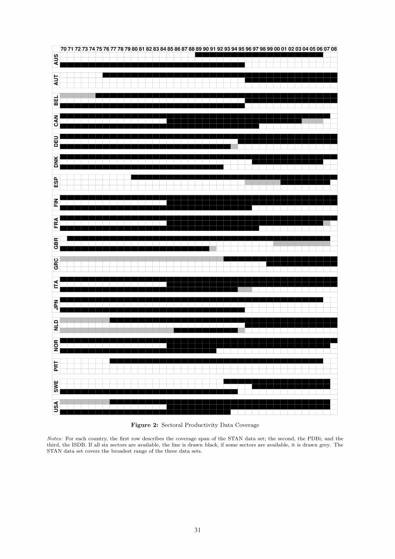
31

70 71 72 73 74 75 76 77 78 79 80 81 82 83 84 85 86 87 88 89 90 91 92 93 94 95 96 97 98 99 00 01 02 03 04 05 06 07 08

0 0 0 0 0 0 0 0 0 0 0 0 0 0 0 0 0 0 0 6 6 6 6 6 6 6 6 6 6 6 6 6 6 6 6 6 6 0 0

0 0 0 0 0 0 0 0 0 0 0 0 0 0 0 0 0 0 0 0 0 0 0 0 0 0 0 0 0 0 0 0 0 0 0 0 0 0 0

6 6 6 6 6 6 6 6 6 6 6 6 6 6 6 6 6 6 6 6 6 6 6 6 6 6 0 0 0 0 0 0 0 0 0 0 0 0 0

0 0 0 0 0 0 6 6 6 6 6 6 6 6 6 6 6 6 6 6 6 6 6 6 6 6 6 6 6 6 6 6 6 6 6 6 6 6 6

0 0 0 0 0 0 0 0 0 0 0 0 0 0 0 0 0 0 0 0 0 0 0 0 0 0 6 6 6 6 6 6 6 6 6 6 6 6 6

0 0 0 0 0 0 0 0 0 0 0 0 0 0 0 0 0 0 0 0 0 0 0 0 0 0 0 0 0 0 0 0 0 0 0 0 0 0 0

5 5 5 5 5 6 6 6 6 6 6 6 6 6 6 6 6 6 6 6 6 6 6 6 6 6 6 6 6 6 6 6 6 6 6 6 6 6 6

0 0 0 0 0 0 0 0 0 0 0 0 0 0 0 0 0 0 0 0 0 0 0 0 0 0 6 6 6 6 6 6 6 6 6 6 6 6 6

6 6 6 6 6 6 6 6 6 6 6 6 6 6 6 6 6 6 6 6 6 6 6 6 6 6 0 0 0 0 0 0 0 0 0 0 0 0 0

6 6 6 6 6 6 6 6 6 6 6 6 6 6 6 6 6 6 6 6 6 6 6 6 6 6 6 6 6 6 6 6 6 6 6 6 6 6 0

0 0 0 0 0 0 0 0 0 0 0 0 0 0 0 6 6 6 6 6 6 6 6 6 6 6 6 6 6 6 6 6 6 6 4 4 4 0 0

6 6 6 6 6 6 6 6 6 6 6 6 6 6 6 6 6 6 6 6 6 6 6 6 6 6 6 6 0 0 0 0 0 0 0 0 0 0 0

6 6 6 6 6 6 6 6 6 6 6 6 6 6 6 6 6 6 6 6 6 6 6 6 6 6 6 6 6 6 6 6 6 6 6 6 6 6 6

0 0 0 0 0 0 0 0 0 0 0 0 0 0 0 0 0 0 0 0 0 0 0 0 0 6 6 6 6 6 6 6 6 6 6 6 6 6 6

6 6 6 6 6 6 6 6 6 6 6 6 6 6 6 6 6 6 6 6 6 6 6 6 3 0 0 0 0 0 0 0 0 0 0 0 0 0 0

6 6 6 6 6 6 6 6 6 6 6 6 6 6 6 6 6 6 6 6 6 6 6 6 6 6 6 6 6 6 6 6 6 6 6 6 6 6 6

0 0 0 0 0 0 0 0 0 0 0 0 0 0 0 0 0 0 0 0 0 0 0 0 0 0 0 6 6 6 6 6 6 6 6 6 6 0 0

6 6 6 6 6 6 6 6 6 6 6 6 6 6 6 6 6 6 6 6 6 6 6 0 0 0 0 0 0 0 0 0 0 0 0 0 0 0 0

0 0 0 0 0 0 0 0 0 0 6 6 6 6 6 6 6 6 6 6 6 6 6 6 6 6 6 6 6 6 6 6 6 6 6 6 6 6 6

0 0 0 0 0 0 0 0 0 0 0 0 0 0 0 0 0 0 0 0 0 0 0 0 0 0 3 3 3 3 3 6 6 6 6 6 6 6 0

0 0 0 0 0 0 0 0 0 0 0 0 0 0 0 0 0 0 0 0 0 0 0 0 0 0 0 0 0 0 0 0 0 0 0 0 0 0 0

6 6 6 6 6 6 6 6 6 6 6 6 6 6 6 6 6 6 6 6 6 6 6 6 6 6 6 6 6 6 6 6 6 6 6 6 6 6 6

0 0 0 0 0 0 0 0 0 0 0 0 0 0 0 6 6 6 6 6 6 6 6 6 6 6 6 6 6 6 6 6 6 6 6 6 6 6 6

6 6 6 6 6 6 6 6 6 6 6 6 6 6 6 6 6 6 6 6 6 6 6 6 6 6 6 0 0 0 0 0 0 0 0 0 0 0 0

6 6 6 6 6 6 6 6 6 6 6 6 6 6 6 6 6 6 6 6 6 6 6 6 6 6 6 6 6 6 6 6 6 6 6 6 6 6 6

0 0 0 0 0 0 0 0 0 0 0 0 0 0 0 6 6 6 6 6 6 6 6 6 6 6 6 6 6 6 6 6 6 6 6 6 6 5 0

6 6 6 6 6 6 6 6 6 6 6 6 6 6 6 6 6 6 6 6 6 6 6 6 6 6 6 6 0 0 0 0 0 0 0 0 0 0 0

0 6 6 6 6 6 6 6 6 6 6 6 6 6 6 6 6 6 6 6 6 6 6 6 6 6 6 6 6 6 6 6 6 6 6 6 6 6 0

0 0 0 0 0 0 0 0 0 0 0 0 0 0 0 0 0 0 0 0 0 0 0 0 0 0 0 0 0 0 5 5 5 5 5 5 5 5 0

6 6 6 6 6 6 6 6 6 6 6 6 6 6 6 6 6 6 6 6 6 2 0 0 0 0 0 0 0 0 0 0 0 0 0 0 0 0 0

1 1 1 1 1 1 1 1 1 1 1 1 1 1 1 1 1 1 1 1 1 1 1 6 6 6 6 6 6 6 6 6 6 6 6 6 6 6 6

0 0 0 0 0 0 0 0 0 0 0 0 0 0 0 0 0 0 0 0 0 0 0 0 0 0 0 0 0 6 6 6 6 6 6 6 6 6 6

0 0 0 0 0 0 0 0 0 0 0 0 0 0 0 0 0 0 0 0 0 0 0 0 0 0 0 0 0 0 0 0 0 0 0 0 0 0 0

6 6 6 6 6 6 6 6 6 6 6 6 6 6 6 6 6 6 6 6 6 6 6 6 6 6 6 6 6 6 6 6 6 6 6 6 6 6 6

0 0 0 0 0 0 0 0 0 0 0 0 0 0 0 6 6 6 6 6 6 6 6 6 6 6 6 6 6 6 6 6 6 6 6 6 6 6 6

6 6 6 6 6 6 6 6 6 6 6 6 6 6 6 6 6 6 6 6 6 6 6 6 6 1 1 0 0 0 0 0 0 0 0 0 0 0 0

6 6 6 6 6 6 6 6 6 6 6 6 6 6 6 6 6 6 6 6 6 6 6 6 6 6 6 6 6 6 6 6 6 6 6 6 6 0 0

0 0 0 0 0 0 0 0 0 0 0 0 0 0 0 0 0 0 0 0 0 0 0 0 0 0 0 0 0 0 0 0 0 0 0 0 0 0 0

6 6 6 6 6 6 6 6 6 6 6 6 6 6 6 6 6 6 6 6 6 6 6 6 6 6 0 0 0 0 0 0 0 0 0 0 0 0 0

4 4 4 4 4 4 4 6 6 6 6 6 6 6 6 6 6 6 6 6 6 6 6 6 6 6 6 6 6 6 6 6 6 6 6 6 6 6 6

0 0 0 0 0 0 0 0 0 0 0 0 0 0 0 0 0 0 0 0 0 0 0 0 0 0 6 6 6 6 6 6 6 6 6 6 6 6 6

4 4 4 4 4 4 4 5 5 5 5 5 5 5 5 5 6 6 6 6 6 6 6 6 6 4 0 0 0 0 0 0 0 0 0 0 0 0 0

6 6 6 6 6 6 6 6 6 6 6 6 6 6 6 6 6 6 6 6 6 6 6 6 6 6 6 6 6 6 6 6 6 6 6 6 6 6 6

0 0 0 0 0 0 0 0 0 0 0 0 0 0 0 6 6 6 6 6 6 6 6 6 6 6 6 6 6 6 6 6 6 6 6 6 6 6 0

6 6 6 6 6 6 6 6 6 6 6 6 6 6 6 6 6 6 6 6 6 6 0 0 0 0 0 0 0 0 0 0 0 0 0 0 0 0 0

0 0 0 0 0 0 0 6 6 6 6 6 6 6 6 6 6 6 6 6 6 6 6 6 6 6 6 6 6 6 6 6 6 6 6 6 6 0 0

0 0 0 0 0 0 0 0 0 0 0 0 0 0 0 0 0 0 0 0 0 0 0 0 0 0 0 0 0 0 0 0 0 0 0 0 0 0 0

0 0 0 0 0 0 0 0 0 0 0 0 0 0 0 0 0 0 0 0 0 0 0 0 0 0 0 0 0 0 0 0 0 0 0 0 0 0 0

0 0 0 0 0 0 0 0 0 0 0 0 0 0 0 0 0 0 0 0 0 0 0 6 6 6 6 6 6 6 6 6 6 6 6 6 6 6 0

0 0 0 0 0 0 0 0 0 0 0 0 0 0 0 0 0 0 0 0 0 0 0 0 0 0 0 6 6 6 6 6 6 6 6 6 6 6 0

6 6 6 6 6 6 6 6 6 6 6 6 6 6 6 6 6 6 6 6 6 6 6 6 6 0 0 0 0 0 0 0 0 0 0 0 0 0 0

3 3 3 3 3 3 3 6 6 6 6 6 6 6 6 6 6 6 6 6 6 6 6 6 6 6 6 6 6 6 6 6 6 6 6 6 6 6 0

0 0 0 0 0 0 0 0 0 0 0 0 0 0 0 6 6 6 6 6 6 6 6 6 6 6 6 6 6 6 6 6 6 6 6 6 6 6 0

6 6 6 6 6 6 6 6 6 6 6 6 6 6 6 6 6 6 6 6 6 6 6 6 0 0 0 0 0 0 0 0 0 0 0 0 0 0 0

AU

SA

UT

BE

LC

AN

DN

KE

SP

FIN

FR

AG

BR

GR

CIT

AJ

PN

NL

DN

OR

PR

TD

EU

SW

EU

SA

Figure 2: Sectoral Productivity Data Coverage

Notes: For each country, the first row describes the coverage span of the STAN data set; the second, the PDBi; and thethird, the ISDB. If all six sectors are available, the line is drawn black, if some sectors are available, it is drawn grey. TheSTAN data set covers the broadest range of the three data sets.

29

32

B Additional Estimation Results

Table 7: Estimation Results with TOT (−1)

Dependent Variable: RERVariables (1) (2) (3)

TFP.TPDBi −0.209∗∗∗

(0.068)TFP.NTPDBi −0.890∗∗∗

(0.321)LP.T STAN −0.117∗∗ −0.101∗∗

(0.055) (0.040)LP.NT STAN −0.090 −0.183∗

(0.102) (0.108)TOT (−1) 0.181 0.275∗∗ 0.342∗∗∗

(0.133) (0.112) (0.043)

LLC Test −9.087∗∗∗ −6.204∗∗∗ −7.319∗∗∗

Kao Test −4.593∗∗∗ −6.487∗∗∗ −5.703∗∗∗

Obs. 181 258 358

Notes: See Table 1 for the definitions of the variables. Panel DOLS estimates in (1)-(3): All FE estimator regressionsinclude country-specific and time-specific dummy variables as well as the first differences of each explanatory variable (1lead/lag). Sample period: 1984-2008 in (1)-(2), and 1971-2008 in (3). Country sample (Appendix A.1): Sample (ii). Theproductivity data stem from the PDBi in (1) and the STAN database in (2)-(3). The robust standard errors proposedby Driscoll and Kraay (1998) are reported in parentheses. LLC test: Cointegration test following MacDonald and Ricci(2007): t-statistic of Levin et al. (2002) (Lag length selection by SIC; Bartlett kernel, Newey-West bandwidth). Kaotest: Cointegration test proposed by Kao (1999): t-statistic (Lag length selection by SIC; Bartlett kernel, Newey-Westbandwidth). ∗/∗∗/∗∗∗ denote significance at the 10%, 5% and 1% levels, respectively.

Table 8: The Balassa Samuelson Effect in Eurozone countries

Dependent Variable: RERVariables (1) (2)

TFP.TPDBi −0.117∗∗∗ −0.082∗∗∗

(0.018) (0.015)TFP.NTPDBi −0.678∗∗∗ −0.473∗∗∗

(0.083) (0.037)TOT 0.470∗∗∗ 0.146∗∗∗

(0.061) (0.026)

LLC Test −6.630∗∗∗ −13.719∗∗∗

Kao Test −1.913∗∗ −1.913∗∗

Obs. 80 104

Notes: See Table 1 for the definitions of the variables. Panel DOLS estimates in (1): All FE estimator regressions includecountry-specific and time-specific dummy variables as well as the first differences of each explanatory variable (1 lead/lag).Sample period: 1995-2008. Country sample: Austria, Belgium, Finland, Germany, France, Italy, Netherlands and Spain.The productivity data stem from the PDBi. The robust standard errors proposed by Driscoll and Kraay (1998) are reportedin parentheses in (1). Group-mean panel FMOLS estimate proposed by Pedroni (2001) in (2). ∗/∗∗/∗∗∗ denote significanceat the 10%, 5% and 1% levels, respectively.

30

33

Table 9: Additional Estimation Results

Dependent Variable: RERVariables (1) (2) (3)

TFP.TPDBi −0.506∗∗∗ −0.392∗∗∗

(0.110) (0.077)TFP.NTPDBi −0.625∗∗ 0.306

(0.286) (0.253)LP.T STAN −0.053

(0.038)LP.NT STAN 0.493∗∗∗

(0.132)TOT 0.349∗∗∗ 0.133∗

(0.096) (0.076)RI 0.036∗∗∗

(0.013)NFA 0.001∗

(0.001)

LLC Test −9.300∗∗∗ −7.757∗∗∗ −7.028∗∗∗

Kao Test −6.854∗∗∗ −5.489∗∗∗ −4.168∗∗∗

Obs. 507 151 125

Notes: See Table 1 for the definitions of the variables. Panel DOLS estimates in (1)-(3): All FE estimator regressionsinclude country-specific and time-specific dummy variables as well as the first differences of each explanatory variable (1lead/lag). Sample period: 1970-2008 in (1), and 1984-2008 in (2)-(3). Country sample (Appendix A.1): Sample (iii) in (1),sample (ii) in (2), and sample (i) in (3). The productivity data stem from the PDBi in (2)-(3) and the STAN database in (1).The robust standard errors proposed by Driscoll and Kraay (1998) are reported in parentheses. LLC test: Cointegrationtest following MacDonald and Ricci (2007): t-statistic of Levin et al. (2002) (Lag length selection by SIC; Bartlett kernel,Newey-West bandwidth). Kao test: Cointegration test proposed by Kao (1999): t-statistic (Lag length selection by SIC;Bartlett kernel, Newey-West bandwidth). ∗/∗∗/∗∗∗ denote significance at the 10%, 5% and 1% levels, respectively.

31

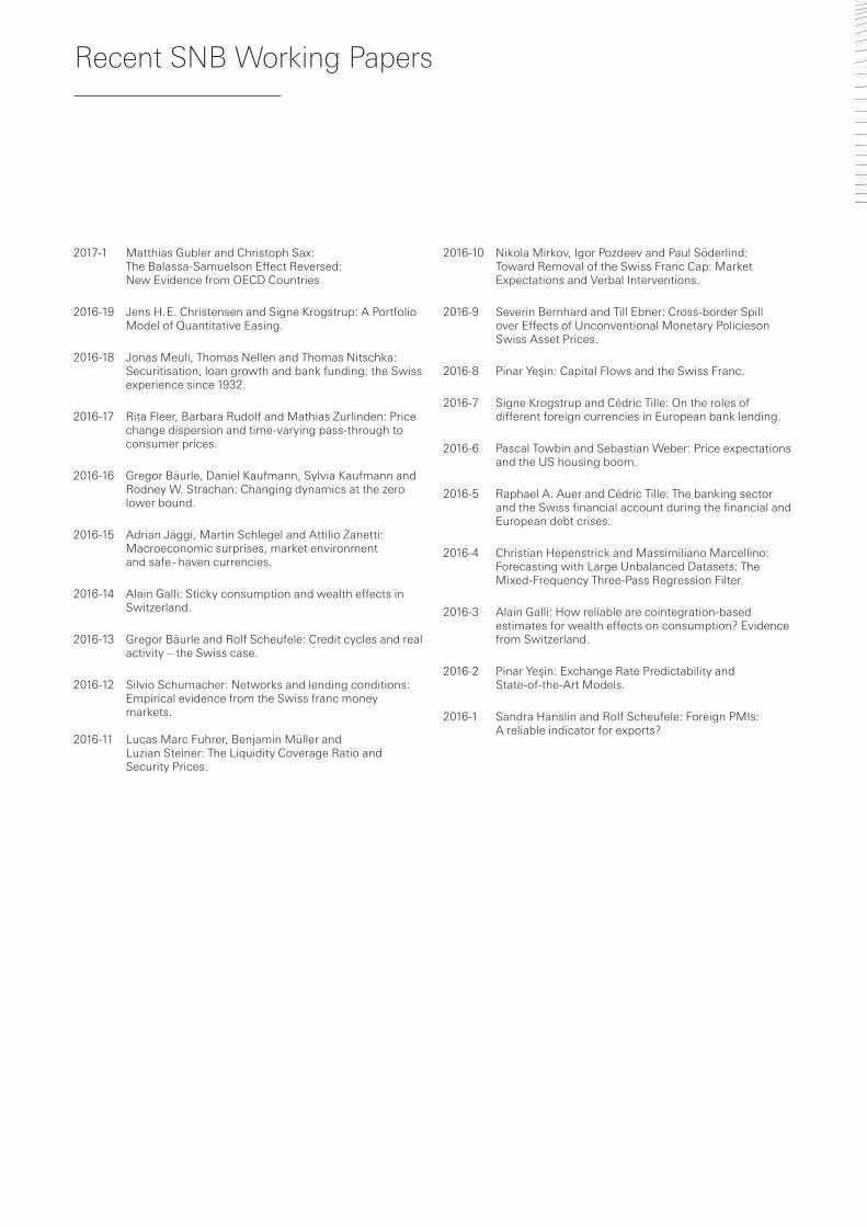
2017-1 MatthiasGublerandChristophSax: TheBalassa-SamuelsonEffectReversed: New Evidence from OECD Countries

2016-19 JensH.E.ChristensenandSigneKrogstrup:APortfolio Model of Quantitative Easing.

2016-18 JonasMeuli,ThomasNellenandThomasNitschka: Securitisation,loangrowthandbankfunding:theSwiss experiencesince1932.

2016-17 RitaFleer,BarbaraRudolfandMathiasZurlinden:Price change dispersion and time-varying pass-through to consumer prices.

2016-16 GregorBäurle,DanielKaufmann,SylviaKaufmannand RodneyW.Strachan:Changingdynamicsatthezero lower bound.

2016-15 AdrianJäggi,MartinSchlegelandAttilioZanetti: Macroeconomic surprises, market environment and safe - haven currencies.

2016-14 AlainGalli:Stickyconsumptionandwealtheffectsin Switzerland.

2016-13 GregorBäurleandRolfScheufele:Creditcyclesandreal activity – the Swiss case.

2016-12 SilvioSchumacher:Networksandlendingconditions: Empirical evidence from the Swiss franc money markets. 2016-11 LucasMarcFuhrer,BenjaminMüllerand LuzianSteiner:TheLiquidityCoverageRatioand Security Prices.

2016-10 NikolaMirkov,IgorPozdeevandPaulSöderlind: TowardRemovaloftheSwissFrancCap:Market Expectations and Verbal Interventions.

2016-9 SeverinBernhardandTillEbner:Cross-borderSpill overEffectsofUnconventionalMonetaryPolicieson SwissAssetPrices.

2016-8 PinarYeşin:CapitalFlowsandtheSwissFranc.

2016-7 SigneKrogstrupandCédricTille:Ontherolesof differentforeigncurrenciesinEuropeanbanklending.

2016-6 PascalTowbinandSebastianWeber:Priceexpectations and the US housing boom.

2016-5 RaphaelA.AuerandCédricTille:Thebankingsector andtheSwissfinancialaccountduringthefinancialand European debt crises.

2016-4 ChristianHepenstrickandMassimilianoMarcellino: ForecastingwithLargeUnbalancedDatasets:The Mixed-FrequencyThree-PassRegressionFilter.

2016-3 AlainGalli:Howreliablearecointegration-based estimatesforwealtheffectsonconsumption?Evidence fromSwitzerland.

2016-2 PinarYeşin:ExchangeRatePredictabilityand State-of-the-ArtModels.

2016-1 SandraHanslinandRolfScheufele:ForeignPMIs: Areliableindicatorforexports?

Recent SNB Working Papers