The Asset Durability Premium

Kai Li and Chi-Yang Tsou∗

August 1st, 2020

Abstract

This paper studies how the durability of assets affects the cross-section of stock returns. More

durable assets incur lowers frictionless user costs but are more “expensive”, in the sense that

they need more down payments making them hard to finance. In recessions, firms become

more financially constrained and prefer “cheaper” less durable assets. As a result, the price of

less durable assets is less procyclical and therefore less risky than that of durable assets. We

provide strong empirical evidence to support this prediction. Among financially constrained

stocks, firms with higher asset durability earn average returns about 5% higher than firms

with lower asset durability. We develop a general equilibrium model with heterogeneous

firms and collateral constraints to quantitatively account for such a positive asset durability

premium.

JEL Codes: E2, E3, G12

Keywords: Durability; financial constraints; collateral, cross-section of stock returns

First Draft: April 8, 2019

∗Kai Li (kaili@ust.hk) is an assistant professor of finance at Hong Kong University of Science and Tech-nology; and Chi-Yang Tsou (bentsou@ust.hk) is a research fellow of finance at Hong Kong University ofScience and Technology. We thank Hengjie Ai, Utpal Bhattacharya, Hui Chen, Andrei Goncalves (MFAdiscussant), Vidhan Goyal, Zhiguo He, Ilan Cooper, Yan Ji, Adriano Rampini, Jialin Yu, Chu Zhang, as wellas the seminar participants at the HKUST, BI Norwegian, Peking University HSBC Business School, andMFA Annual Meeting, SJTU-UCL Macro-finance Workshop for their helpful comments. Kai Li gratefullyacknowledges the General Research Fund of the Research Grants Council of Hong Kong (Project Number:16502617) for financial support. The usual disclaimer applies.

1 Introduction

Durability is an essential feature of capital, and varies dramatically across types of assets.

How does asset durability affect firms’ equity risks and, in turn, the cost of capital? Rampini

(2019) argues that asset durability significantly affects financing. In particular, more durable

assets incur lower frictionless user costs but are more “expensive”, in the sense that they

need higher down payments making more durable assets hard to finance. In this paper,

we build this insight into a canonical macroeconomic model with collateral constraints, and

demonstrate that asset durability have profound implications on the risk profile on the asset

side of firms’ balance sheets, exactly through the impact of asset durability on the debt

financing on the liability side.

A common prediction of a macro finance model with financial frictions is that financial

constraints exacerbate economic downturns because they are more binding in bad time. In

recessions, firms become more financially constrained and collectively prefer “cheaper” less

durable assets that require less down payments. This creates a general equilibrium effect

that the price of less durable assets is less procyclical and therefore less risky than that of

durable assets. In sum, our theory predicts that less durable assets are less risky than more

durable assets. We evaluate this mechanism through the lens of the cross-section of equity

returns. In particular, our theory suggests that a firm holding a larger fraction of less durable

assets commands a lower expected return, since less durable assets provide a hedge against

the aggregate risks, especially in recessions when firms become more financially constrained.

To examine the empirical relationship between asset durability and expected returns, we

first construct a measure of firm’s asset durability. Asset durability of capital can be measured

in two ways, either by modeling with geometric depreciation rates or with a finite service life,

as in Rampini (2019). Our paper measures a firm’s asset durability as the value-weighted

average of the durability of the different types of assets owned by the firm.

Consistent with the theoretical prediction in our model, Our empirical study focuses

on financially constrained firms. We construct five portfolios univariate sorted on firms’

durability relative to firms’ industry peers using the U.S. data on publicly traded firms. We

show that the asset durability return spread, that is, the returns of a long high durability

firms and short low durability firms portfolio among the financially constrained firms is

statistically significant. Our empirical finding documents that the spread between the highest

durability quintile portfolio and the lowest durability quintile portfolio is on average close

to 4-7% per annum within the subset of financially constrained firms. We call the asset

durability premium as the difference in average portfolio returns between the highest and

2

lowest portfolio sorted by the asset durability measure. A high-minus-low strategy based on

the asset durability spread delivers an annualized Sharpe ratio of 0.59, comparable to that

of the market portfolio. Moreover, according the asset pricing test shown in Section 6.2,

the alphas remain significant even after controlling for Fama and French (2015) five factors

or Hou, Xue, and Zhang (2015) (HXZ hereafter) q-factors, respectively. The evidence on

the durability spread strongly supports our theoretical prediction that the durable capital is

more risky and therefore earn a higher expected return than the non-durable capital.

We also empirically review the ability of firm-level durability to predict the cross-sectional

stock returns using monthly Fama and MacBeth (1973) regressions. This analysis allows us

to control for an extensive list of firm characteristics that predict stock returns. The slope

coefficient associated with the firm’s lagged durability is both economically and statistically

significant. To be concrete, in the baseline specification in which we also control for the

financial leverage of the firm, a one-unit standard deviation increase in the firm’s durability

is associated with an increase of 2.13% in firms’ expected (future) stock return. For the

robustness, we verify that the positive durability-return relation is not driven by other known

predictors which are seemingly correlated with the durability measure.

To quantify the effect of asset durability on the cross-section of expected returns, we

develop a general equilibrium model with heterogeneous firms and financial constraints. As

in Kiyotaki and Moore (1997) and Gertler and Kiyotaki (2010), lending contracts can not

be fully enforced and therefore require collateral. In our model, assets with different levels

of asset durability are traded, and firms with higher financing needs but low net worth

endogenously acquire less durable assets. This is because, as in Rampini (2019), a durable

capital incurs a lower frictionless user cost but is costly with a higher upfront down payment

and, therefore, hard to finance. In the economic downturns, firms become more financially

constrained and prefer cheaper less durable capital collectively and in turn creates a general

equilibrium price effect. In particular, firms with high productivity and low net worth face

higher financing needs in equilibrium and tend to acquire cheaper assets (i.e., less durable

assets with lower down payments). As a result, the price of less durable capital is less

procyclical and, therefore, less risky than that of durable capital. In the constrained efficient

allocation in our model, the heterogeneity in productivity and net worth translates into the

heterogeneity in asset durability across firm assets. In this setup, we show that, at the

aggregate level, more durable capital requires higher expected returns in equilibrium, and,

in the cross-section, firms with high asset durability earn high risk premia.

In our quantitative analysis, we show that our model, when calibrated to match the con-

ventional macroeconomic quantity dynamics and asset pricing moments, is able to generate

3

significant asset durability spread. As consistent with the data, firms with higher asset dura-

bility exhibit higher financial leverages. Quantitatively, our model matches the empirical

relationship between asset durability, leverage, and expected returns in the data reasonably

well.

On the empirical side, we further provide empirical evidence that directly support model

implications. First, we document that the price of capital with higher durability exhibits

higher sensitivities to the aggregate macroeconomic shocks. Second, we show that high

asset durability firms have significant higher cash flow betas with respect to the aggregate

TFP and GDP growth shocks. Third, we further follow the standard empirical procedure

to estimate stochastic discount factor using the generalized method of moments (GMM),

and show that the aggregate TFP and GDP growth shocks are significantly positively priced

among durability-sorted portfolios. Firms with high durability are more positively exposed

to these aggregate shocks and, therefore, demand for higher expected returns, consistent with

our model interpretation.

1.1 Related literature

Our paper builds on the corporate finance literature that emphasizes the importance of

collateral for firms’ capital structure decisions. Albuquerque and Hopenhayn (2004) study

dynamic financing with limited commitment, Rampini and Viswanathan (2010, 2013) develop

a joint theory of capital structure and risk management based on firms’ asset collateraliz-

ability. Schmid (2008) considers the quantitative implications of dynamic financing with

collateral constraints. Nikolov et al. (2018) studies the quantitative implications of various

sources of financial frictions on firms’ financing decisions, including the collateral constraint.

Falato et al. (2013) provide empirical evidence for the link between asset collateralizability

and leverage in aggregate time series and in the cross section. Our paper departs from the

above literature in three important dimensions: first, we explicitly study firms’ optimal asset

acquisition decision among assets with different durability under the context of a collateral

constraint, as in Rampini (2019). However, different from Rampini (2019), we bring an asset

durability decision into a general equilibrium framework, take aggregate shocks into accounts,

and then study the asset pricing implications of such a decision on the asset side of firms’

balance sheets through the lens of the cross-sectional stock returns.

Our study builds on the large macroeconomics literature studying the role of credit market

frictions in generating fluctuations across the business cycle (see Quadrini (2011) and Brun-

nermeier et al. (2012) for extensive reviews). The papers that are most related to ours are

4

those emphasizing the importance of borrowing constraints and contract enforcements, such

as Kiyotaki and Moore (1997, 2012), Gertler and Kiyotaki (2010), He and Krishnamurthy

(2013), Brunnermeier and Sannikov (2014), and Elenev et al. (2018). Gomes et al. (2015)

studies the asset pricing implications of credit market frictions in a production economy. We

allow firms to optimally choose their asset durability, and study the implications of durable

versus less durable capital on the cross-section of expected returns.

Our paper belongs to the literature of production-based asset pricing, for which Kogan

and Papanikolaou (2012) provide an excellent survey. From the methodological point of

view, our general equilibrium model allows for a cross section of firms with heterogeneous

productivity and is related to previous work including Gomes et al. (2003), Garleanu et al.

(2012), Ai and Kiku (2013), and Kogan et al. (2017). Compared to the above papers, our

model incorporates financial frictions and study their asset pricing implications. In this

regard, our paper is closest related to Ai, Li, Li, and Schlag (2019) and Li and Tsou (2019),

which both use a similar model framework and aggregation technique to study stock returns

and the asset collateralizability and leasing versus secure lending, respectively. Ai, Li, Li, and

Schlag (2019) shows that more collateralizable assets provide an insurance against aggregate

shocks, because these assets help relax the collateral constraint, especially in recessions when

the financial constraint becomes more binding.

Our paper is related to a recent literature on the duration premium in the cross-section.

Papers, including Goncalves (2019), Gormsen and Lazarus (2019) and Chen and Li (2018),

show that firms with longer cash flow duration earn a lower average return than those with

longer cash flow duration. Our paper is consistent with this evidence. In our model, other

things being equal, firms that experienced a history of positive productivity shocks have a

internal cash flow and optimally choose to obtain higher asset durability. Therefore, in the

model, a history of high productivity shocks is associated with higher asset durability, higher

ROE and but shorter cash flow duration. As shown in Table C.1, this feature of our model

is consistent with the pattern in the data. In particular, higher asset durability firms display

shorter Dechow et al. (2004) cash flow duration but high expected return, in line with the

short cash flow premium documented in the above papers.

Our paper is also connected to the broader literature linking investment to the cross-

section of expected returns. Zhang (2005) provides an investment-based explanation for the

value premium. Li (2011) and Lin (2012) focus on the relationship between R&D investment

and expected stock returns. Eisfeldt and Papanikolaou (2013) develop a model of organi-

zational capital and expected returns. Belo, Lin, and Yang (2018) study implications of

equity financing frictions on the cross-section of stock returns. Tuzel (2010) documents a

5

positive relation between firms’ real estate holding and expected returns, and she proposes

an adjustment cost explanation. Our paper focuses on a broader definition of asset dura-

bility, in which real estate is one particular kind of durable capital. Moreover, we propose

a complementary financial constraint explanation. In the data, we find the asset durability

premium is more significant among the financially constrained firms, which directly supports

our model mechanism.

The rest of our paper is organized as follows. We summarize our empirical results on

the relationship between asset durability and expected returns in Section 2. We introduce

a general equilibrium model with collateral constraints in Section 3 and analysis the asset

pricing implications in Section 4. In Section 5, we provide a quantitative analysis of our

model. Section 6 provides supporting evidence of the model. Section 7 concludes. Details

on data construction are delegated to the Appendix B. In Appendix C, we further provide

some additional empirical evidence to establish the robustness.

2 Empirical Facts

This section provides some cross-sectional and aggregate evidence that highlight the asset

durability as an important determinant of the cross-section of stock returns, especially for

for financially constrained firms.

2.1 Measuring Asset Durability

To empirically examine the link between asset durability and expected returns and test

our theoretical prediction, we need to construct a separate measure of asset durability with

respect to physical assets (i.e., equipment, structures) and intangible assets (i.e., intellectual

property and product). We measure an asset’s durability as its service life by calculating the

reciprocal of the asset’s depreciation rate.

We construct the measure of asset durability using the Bureau of Economic Analysis

(BEA) fixed asset table with non-residential detailed estimates for implied rates of depreci-

ation and net capital stocks at fixed cost (hereafter referred to as the ”BEA table”).1 The

table breaks down depreciation rate on equipment, structures, and intellectual property and

1Our data is provided by the Bureau of Economic Analysis (BEA) fixed asset table with non-residentialdetailed estimates for implied rates of depreciation and net capital stocks at fixed cost. This table breaks downimplied rates of depreciation and net capital stocks into a variety of asset categories for a broad cross-sectionof industries.

6

product by 72 assets for 63 industries2, covering virtually all economic sectors in the United

States.3

Constructing the Industry- and Firm-level Asset Durability Measure

Given the BEA table with implied rates of depreciation, the durability of asset h employed

by industry j in year t is computed as asset h’s service life (i.e., the reciprocal of asset h’s

depreciation rate). We value-weight the asset-level durability across the 71 assets (equipment

and structures) in the BEA table to obtain an industry-level asset durability index:

Asset DurabilityKj,t =71∑h=1

wh,j,t × Asset Durability ScoreKh,j,t, (1)

where Asset DurabilityKj,t is a measure of asset durability for industry j in year t, wh,j,t rep-

resents industry j’s capital stocks on asset h divided by its total capital stocks in year t from

the BEA table, and Asset Durability ScoreKh,j,t is the durability score of asset h employed

by industry j in year t. The resulting asset durability index represents a relative asset dura-

bility ranking of each industry’s asset composition of tangible assets. On the other hand, we

compute the asset durability of the intellectual property and product, Asset DurabilityHj,t,

as the the reciprocal of industry j’s depreciation rate in year t.4

Further, we construct a firm-level measure of asset durability with respect to tangible

and intangible assets as the value-weighted average of industry-level asset durability indices

across business segments in which the firm operates:

Asset DurabilityKi,t =

ni,t∑j=1

wi,j,t × Asset DurabilityKj,t,

Asset DurabilityHi,t =

ni,t∑j=1

wi,j,t × Asset DurabilityHj,t, (2)

where Asset DurabilityKi,t (Asset DurabilityHi,t) is firm i’s asset durability of tangible (intan-

gible) capital, ni,t is the number of industry segments, and wi,j,t is industry segment j’s sales

divided by the total sales for firm i in year t, and Asset DurabilityKj,t (Asset DurabilityHj,t)

2We do not include detailed assets of the intellectual property and product because of missing data issue.Therefore, we consider the depreciation rate of the intellectual property and product at industry-level. Landis not included in the BEA non-residential asset categories. We assume land has infinite durability acrossindustries.

3The industry classification employed by the BEA is based on the 1997 North American Industry Classi-fication System (NAICS). Therefore, we match the 63 BEA industries with Compustat firms using NAICScode.

4In this paper, we use the terms ”intellectual property and product” and ”intangible” interchangeably.

7

is the asset dutiability of industry j in year t for the type-K (type-H) computed as equation

(1).

Now we obtain firm i’s asset durability of equipment and structures and that of intellectual

property and product, respectively, and value-weight these two types of asset durability by

their capital stocks, which refer to firm i’s tangible capital PPEGTi,t and intangible capital

INTANi,t in year t, respectively, where wi,t denotes firm i’s relative weight of these two types

of capital at time t.5

Asset Durabilityi,t = wi,t × Asset DurabilityKi,t + (1− wi,t)× Asset DurabilityHi,t. (3)

In the main empirical analysis, we employ this firm-level measure, which is likely to

provide more refined across-firm variation in asset durability than the industry-level one.6

Due to the availability of the asset durability measure interacting with the U.S. data on

publicly traded firms, our main analysis is then performed for the 1978 to 2016 period.

2.2 Asset Durability and Financial Constraints

Consistent with Rampini (2019), our model predict financial constraint is critical for firms

to determine the composition of durable and less durable capital. With the firm level asset

durability measure, we provide a first evidence that financial constraint is an important

determinant for firms’ asset durability decision, which supports both Rampini (2019) and

our theoretical prediction.

In this subsection, we show that a firm’s asset durability is increasing in its financial

constraints. The asset durability increases in financial constraint since the capacity of exter-

nal financing is declining. The empirical implication is that measures of financial constraint

(i.e., non-dividend payment dummy7, SA index, WW index) should be negatively related to

the asset durability. Moreover, to the extent that profitability contributes to internal funds,

profitability should be positively related to the asset durability. Therefore, we examine these

empirical predictions as follows.

[Place Table 1 about here]

The financial variables that we use are motivated by the empirical predictions of our mode,

5Details in the measurement of intangibles refer to Ai, Li, Li, and Schlag (2019).6Our asset durability measure is robust to the measure constructed by using depreciation expenditure in

Compustat.7In contrast to dividend payment dummy (DIV), non-dividend payment dummy (Non-Div) is whether a

firm pays no dividend.

8

as well as by existing literature. We expect to find negative coefficients on non-dividend

payment dummy, SA index, WW index, and a positive coefficient on profitability. As our

model shows in later sections, variables that indicate that a firm is financially constrained,

places a high value on internal fund, and, therefore, endogenously choose “cheaper” less

durable assets, which is consistent with the negative correlation of a firm’s financial constraint

with its optimal decision for high durable assets.

Specification 1-4 of Table 1 reports the results of a univariate regression for each of the

financial constraint or profitability, and specification 5-7 reports the results for a multi-

variate regression controlling for other fundamentals. Non-dividend dummy is significantly

negatively related to asset durability both univariate and multivariate specification, which

suggests that payout policy seems to be a direct measure of the value of internal funds.

Such a negative relation to asset durability remains robust when we replace the non-dividend

payment dummy by alternative financial constraint measures. Likewise, other financial con-

straint measure, SA and WW index, are also significantly negative related to asset durability,

which is consistent with our theory that constrained firms prefer less durable assets and tend

to hold larger internal funds to insure future negative aggregate shocks. Taking all together,

results in Table 1 motivate us to shift our attention to financially constrained firms and

further investigate the asset pricing implications in the following sections.

2.3 Asset Durability and Leverage

In Table 2, we construct the firm-level durability measure and report summary statistics of

asset durability and book leverage for the aggregate and the cross-sectional firms in Compu-

stat.

[Place Table 2 about here]

Panel A reports the statistics of the financially constrained firm group versus its uncon-

strained counterpart. The constraint is measured by the dividend payment dummy (Farre-

Mensa and Ljungqvist (2016), DIV hereafter).8 Panel A presents two salient observations.

First, the average of asset durability among financially constrained firms (12.66) is signif-

icantly lower than that of the unconstrained firms (16.54); that is to say, financially con-

strained firms use capital with higher durability (lower depreciation rate). Second, the aver-

age book leverage of constrained firms (0.24) is lower than that of unconstrained counterpart

(0.33).

8We tried other financial constrained measures, including SA index, credit rating, and WW index. Thesefour proxies show consistent results empirically.

9

In panel B, we further sort financially constrained firms in the Compustat into five quin-

tiles based on their asset durability relative to their industry peers as NAICS 3-digit industry

classifications, and report firm characteristics across five quintiles. First, we observe a large

dispersion in the average asset durability (depreciation), ranging from 7.69 (0.19) in the low-

est quintile (Quintile L) to a ratio as much as 18.00 (0.11) in the highest quintile (Quintile

H). Second, the book leverage is upward sloping from the lowest to the highest asset dura-

bility sorted portfolio. From these findings in Table 2, we recognize that asset durability can

be a critical determinant of external financing activities for the constrained group, and that

it is the first-order determinant of the capital structure on the firms’ liability side. In the

next section, we will present evidence to show that asset durability also plays an important

role on firms’ asset side, as reflected by equity returns across firms with heterogenous asset

durability.

2.4 Asset Durability and Expected Returns

We zoom in on on the subset of financially constrained firms, consistent with our theory that

firms’ asset valuations contain a non-zero Lagrangian multiplier component. We consider

four alternative measures for the degree to which a firm is financially constrained: the div-

idend payment dummy (Farre-Mensa and Ljungqvist (2016), DIV hereafter), the Size-Age

index (Hadlock and Pierce (2010), SA index hereafter), the credit rating (Farre-Mensa and

Ljungqvist (2016), Rating hereafter), and the Whited-Wu index (Whited and Wu (2006),

Hennessy and Whited (2007), WW index hereafter). A firm is classified as a financially

constrained firm if its dividend payment is zero, if its credit rating is missing, or if its WW

(SA) index is higher than the median in a given year.

To investigate the link between asset durability and future stock returns in the cross-

section, we construct five portfolios sorted on a firms’s current asset durability and report

the portfolio’s post-formation average stock returns. We construct the durability at an annual

frequency as described in Section 2.1. We focus on annual rebalancing (as opposed to monthly

rebalancing) to minimize transaction costs of the investment strategy. At the end of June of

year t from 1978 to 2017, we rank firms by asset durability relative to their industry peers and

construct portfolios as follows. Specifically, we sort all firms with positive asset durability in

year t-1 into five groups from low to high within the corresponding NAICS 3-digit industries.

As a result, we have industry-specific breaking points for quintile portfolios for each June. We

then assign all firms with positive asset durability in year t-1 into these portfolios. Thus, the

low (high) portfolio contains firms with the lowest (highest) asset durability in each industry.

To examine the asset durability-return relation, we form a high-minus-low portfolio that

10

takes a long position in the high durability portfolio and a short position in the low asset

durability portfolio.

After forming the six portfolios (from low to high and high-minus-low), we calculate the

value-weighted monthly returns on these portfolios over the next twelve months (July in year

t to June in year t+1). To compute the portfolio-level average excess stock return in each

period, we weight each firm in the portfolio by the size of its market capitalization at the time

of portfolio formation. This weighting procedure enables us to give relatively more weight to

the large firms in the economy and hence it minimizes the effect of the very small firms (and

hence potentially difficult to trade) on the results (also note that we drop firms with fewer

than 1 million assets or sales from the sample to further decrease the influence of the small

firms on our results).

[Place Table 3 about here]

In Panel A (Panel B) of Table 3, the top row presents the annualized average excess stock

returns (E[R]-Rf, in excess of the risk free-rate), standard deviations, and Sharpe ratios of

the five portfolios sorted on asset durability. With Table 3, we show that, consistent with

our model, a firm’s asset durability forecasts stock returns. Firms with currently low asset

durability earn subsequently lower returns, on average, than firms with currently high asset

durability.

Table 3 presents the result that the average excess returns on the first five portfolios

increase with asset durability. In the first panel of Panel A, the average excess return for

firms with high asset durability (Portfolio H) is higher on an annualized basis than that

with low asset durability (Portfolio L). Moreover, the average excess return on the high-

minus-low portfolio is 6.93% with statistical significance with a t-value of 2.86 and a Sharpe

ratio 0.59. The difference in returns is economically large and statistically significant. We

find the positive asset durability-return relation and statistical significance on the long-short

portfolio. We call the return spread of a long-short high-minus-low (Portfolio H-L) strategy

the durability premium. The premium is robust with respect to the alternative measure of

financial constraint, as can be seen from the second to the fourth panel. In Panel B, we

find that the average excess returns on five portfolios increase with durability; however, the

long-short portfolio return is amount to 1.44% and statistically insignificant.

Overall, the evidence on the asset durability spread among financially constrained firms

strongly supports our theoretical prediction that more durable assets are more risky and,

therefore, are expected to earn higher expected returns. In the following section, we develop

a general equilibrium model with heterogeneous firms and financial constraints to formalize

11

the above intuition and to quantitatively account for the positive asset durability premium.

3 A General Equilibrium Model

In this section, we describe the ingredients of our quantitative model of the asset durability

spread. The aggregate aspect of the model is intended to follow standard macro models

with collateral constraints such as Kiyotaki and Moore (1997) and Gertler and Kiyotaki

(2010). We allow for heterogeneity in the durability of assets as in Rampini (2019). The key

additional elements in the construction of our theory are idiosyncratic productivity shocks

and firm entry and exit. These features allow us to generate quantitatively plausible firm

dynamics in order to study the implications of asset durability for the cross-section of equity

returns.

3.1 Households

Time is infinite and discrete. The representative household consists of a continuum of workers

and a continuum of entrepreneurs. Workers (entrepreneurs) receive their labor (capital)

incomes every period and submit them to the planner of the household, who make decisions

for consumption for all members of the household. Entrepreneurs and workers make their

financial decisions separately.9

The household ranks the utility of consumption plans according to the following recursive

preference as in Epstein and Zin (1989):

Ut =

{(1− β)C

1− 1ψ

t + β(Et[U1−γt+1 ])

1− 1ψ

1−γ

} 1

1− 1ψ

,

where β is the time discount rate, ψ is the intertemporal elasticity of substitution, and γ is

the relative risk aversion. As we will show later in the paper, together with the endogenous

growth and long run risk, the recursive preference in our model generates a volatile pricing

kernel and a sizable equity premium as in Bansal and Yaron (2004).

In every period t, the household purchases the amount Bi,t of risk-free bonds from en-

trepreneur i, from which she will receive Bi,tRf,t+1 next period, where Rf,t+1 denotes the

risk-free interest rate from period t to t + 1. In addition, the household receives capital in-

9According to Gertler and Kiyotaki (2010), we make the assumption that household members make jointdecisions on their consumption to avoid the need to keep the distribution of entrepreneur income as an extrastate variable.

12

come Πi,t from entrepreneur i. We assume that the labor market is frictionless, and therefore

the labor income from worker members is WtLt. The household budget constraint at time t

can therefore be written as

Ct +

∫Bi,tdi = WtLt +Rf,t

∫Bi,t−1di+

∫Πi,tdi.

LetMt+1 denote the the stochastic discount factor implied by household optimization. Un-

der recursive utility, the stochastic discount factor denotes as, Mt+1 = β(Ct+1

Ct

)− 1ψ

(Ut+1

Et[U1−γt+1 ]

11−γ

) 1ψ−γ

,

and the optimality of the intertemporal saving decisions implies that the risk-free interest

rate must satisfy

Et[Mt+1]Rf,t+1 = 1.

3.2 Entrepreneurs

There is a continuum of entrepreneurs in our economy indexed by i ∈ [0, 1]. Entrepreneurs

are agents operating productive ideas. An entrepreneur who starts at time 0 draws an idea

with initial productivity z and begins the operation with an initial net worth N0. Under our

convention, N0 is also the total net worth of all entrepreneurs at time 0 because the total

measure of all entrepreneurs is normalized to one.

Let Ni,t denote entrepreneur i’s net worth at time t, and let Bi,t denote the total amount

of risk-free bond the entrepreneur issues to the household at time t. Then the time-t budget

constraint for the entrepreneur is given as

qd,tKdi,t+1 + qnd,tK

ndi,t+1 = Ni,t +Bi,t. (4)

In equation (4) we assume that two types of capital, Kd and Knd, differ in their asset

durability. That is, the former capital is more durable, while the latter capital is less durable.

For the brevity of reference, we denote these two types of capital with a superscript d

for durable and nd for non-durable, respectively. These two types of capital depreciate

at geometric depreciation rates δd < δnd each period, with δh ∈ (0, 1), for h ∈ {d, nd}. We

use qd,t and qnd,t to denote their prices at time t, respectively. Kdi,t+1 and Knd

i,t+1 are the

amount of capital that entrepreneur i purchases at time t, which can be used for production

over the period from t to t + 1. We assume that the entrepreneur only has access to risk-

free borrowing contracts, i.e., we do not allow for state-contingent debt. At time t, the

entrepreneur is assumed to have an opportunity to default on his contract and abscond with

13

1− θ of both types of capital. Because lenders can retrieve a θ fraction of the type-j capital

upon default, borrowing is limited by

Bi,t ≤ θ∑

h∈{d,nd}

qh,tKhi,t+1. (5)

Note that in the collateral constraint (5) we assume both types of capital have the same

collateralizability parameter θ. This is an assumption we maintain in order to single out

the effect of asset durability. In Rampini (2019) and in reality, durability could also simul-

taneously affect collateralizability. For instance, in Rampini (2019), he assumes a collateral

constraint of the form Bi,t ≤ θ∑

h∈{d,nd}

qh,tKhi,t+1 (1− δh), in which the effective collateraliz-

ability becomes θ (1− δh) and more durable capital (i.e. lower δh) is more collateralizable.

In our paper, there is a critical distinction between the durability and the collateraliz-

ability of an asset. According to Ai et al. (2019), an asset with a higher colllateralizability

lowers the riskiness of assets, as an insurance to aggregate shocks by relaxing the financing

constraint. However, unlike that of the asset collateralizability, the mechanism of asset dura-

bility affects not only the duration of asset but also the price of the underlying asset. In our

model, an asset with a longer duration is more expensive, incurs a higher down payment,

therefore, is more difficult to finance, as highlighted in Rampini (2019). Such the mechanism

implies that the price of more durable assets is more sensitive to aggregate shocks; that is to

say, assets with longer duration embody higher riskiness than those with shorter duration.

In the quantitative part of our paper, we also consider a variation of the model with Rampini

(2019) type of collateral constraint in which durability simultaneously affects colateralizabil-

ity, we show that quantitatively the net effect of the asset durability is to raise the riskiness

of firm assets. In summary, our model in this paper explicitly distinguishes asset durability

from asset collateralizability and predicts that asset durability could increase the riskiness of

the underlying asset by impeding financing. Moreover, we show that our theoretical predic-

tion is empirically plausible in terms of testable implications on the cross-section of equity

returns.

From time t to t + 1, the productivity of entrepreneur i evolves according to the law of

motion

zi,t+1 = zi,teεi,t+1 , (6)

where εi,t+1 is a Gaussian shock with mean µε and variance σ2ε, assumed to be i.i.d. across

agents i and over time. We use π(At+1, zi,t+1, K

di,t+1, K

ndi,t+1

)to denote entrepreneur i’s equi-

librium profit at time t + 1, where At+1 is aggregate productivity in period t + 1, and zi,t+1

14

denotes entrepreneur i’s idiosyncratic productivity. The specification of the aggregate pro-

ductivity processes will be provided later in Section 5.1.

In each period, after production, the entrepreneur experiences a liquidation shock with

probability λ, upon which he loses his idea and needs to liquidate his net worth to return it

back to the household.10 If the liquidation shock happens, the entrepreneur restarts with a

draw of a new idea with initial productivity z and an initial net worth χNt in period t + 1,

where Nt is the total (average) net worth of the economy in period t, and χ ∈ (0, 1) is a

parameter that determines the ratio of the initial net worth of entrepreneurs relative to that

of the economy-wide average. Conditional on no liquidation shock, the net worth Ni,t+1 of

entrepreneur i at time t+ 1 is determined as

Ni,t+1 = π(At+1, zi,t+1, K

di,t+1, K

ndi,t+1

)+ (1− δd) qd,t+1K

di,t+1

+ (1− δnd) qnd,t+1Kndi,t+1 −Rf,t+1Bi,t. (7)

The interpretation is that the entrepreneur receives the profit π(At+1, zi,t+1, K

di,t+1, K

ndi,t+1

)from production. His capital holdings depreciate at rate δh, and he needs to pay back the

debt borrowed from last period plus interest, amounting to Rf,t+1Bi,t.

Because of the fact that whenever a liquidity shock occurs, entrepreneurs submit their net

worth to the household who chooses consumption collectively for all members, entrepreneurs

value their net worth using the same pricing kernel as the household. Let V it denote the value

function of entrepreneur i. It must satisfy the following Bellman equation:

V it = max

{Kdi,t+1,K

ndi,t+1,Ni,t+1,Bi,t}

Et[Mt+1{λNi,t+1 + (1− λ)V i

t+1 (Ni,t+1)}], (8)

subject to the budget constraint (4), the collateral constraint (5), and the law of motion of

Ni,t+1 given by (7).

We use variables without an i subscript to denote economy-wide aggregate quantities.

The aggregate net worth in the entrepreneurial sector satisfies

Nt+1 = (1− λ)

[π(At+1, K

dt+1, K

ndt+1

)+ (1− δd) qd,t+1K

dt+1

+ (1− δnd) qnd,t+1Kndt+1 −Rf,t+1Bt

]+ λχNt, (9)

where π(At+1, K

dt+1, K

ndt+1

)denotes the aggregate profit of all firms.

10This assumption effectively makes entrepreneurs less patient than the household and prevents them fromsaving their way out of the financial constraint.

15

3.3 Production

Final Output With zi,t denoting the idiosyncratic productivity for firm i at time t,

output yi,t of firm i at time t is assumed to be generated through the following production

technology:

yi,t = At[z1−νi,t

(Kdi,t +Knd

i,t

)ν]αL1−αi,t (10)

In our formulation, α is the capital share, and ν is the span of control parameter as in Atkeson

and Kehoe (2005). Note that durable and non-durable capital are perfect substitutes in

production. This assumption is made for tractability.

Firm i’s profit at time t, π(At, zi,t, K

di,t, K

ndi,t

)is given as

π(At, zi,t, K

di,t, K

ndi,t

)= max

Li,tyi,t −WtLi,t,

= maxLi,t

At[z1−νi,t

(Kdi,t +Knd

i,t

)ν]αL1−αi,t −WtLi,t, (11)

where Wt is the equilibrium wage rate, and Li,t is the amount of labor hired by entrepreneur

i at time t.

It is convenient to write the profit function explicitly by maximizing out labor in equation

(11) and using the labor market clearing condition∫Li,tdi = 1 to get

Li,t =z1−νi,t

(Kdi,t +Knd

i,t

)ν∫z1−νi,t

(Kdi,t +Knd

i,t

)νdi, (12)

so that entrepreneur i’s profit function becomes

π(At, zi,t, K

di,t, K

ndi,t

)= αAtz

1−νi,t

(Kdi,t +Knd

i,t

)ν [∫z1−νi,t

(Kdi,t +Knd

i,t

)νdi

]α−1

. (13)

Given the output of entrepreneur i, yi,t, from equation (10), the total output of the economy

is given as

Yt =

∫yi,tdi,

= At

[∫z1−νi,t

(Kdi,t +Knd

i,t

)νdi

]α. (14)

Capital Goods We assume that capital goods are produced from a constant-return-

to-scale and convex adjustment cost function G(I,Kd +Knd

). That is, one unit of the

investment good costs G(I,Kd +Knd

)units of consumption goods. Therefore, the aggregate

16

resource constraint is

Ct + It +G(It, K

dt +Knd

t

)= Yt. (15)

Without loss of generality, we assume that G(It, K

dt +Knd

t

)= g

(It

Kdt +Knd

t

)(Kd

t +Kndt ) for a

convex function g.

For model tractability, we assume that at the aggregate level, the proportion of two types

of capital is fixed, that is,Kdt

Kt= ζ, and

Kndt

Kt= 1− ζ. In order to achieve a fixed proportion,

we need to specify φt and 1− φt as the fractions of the new investment goods used for type-

d and type-nd capital, respectively, and φt = (δnd − δd) ζ (1− ζ) KtIt

+ ζ. This is another

simplification assumption for model tractability. It implies that, at the aggregate level, the

ratio of type-d to type-nd capital is always equal to ζ/ (1− ζ), and thus the total capital

stock of the economy can be summarized by a single state variable 11. The aggregate stocks

of type-d and type-nd capital satisfy

Kdt+1 = (1− δd)Kd

t + φtIt (16)

Kndt+1 = (1− δnd)Knd

t + (1− φt) It. (17)

4 Equilibrium Asset Pricing

4.1 Aggregation

Our economy is one with both aggregate and idiosyncratic productivity shocks. In general,

we would have to use the joint distribution of capital and net worth as an infinite-dimensional

state variable in order to characterize the equilibrium recursively. In this section, we present a

aggregation result as developed in Ai, Li, Li, and Schlag (2019), and show that the aggregate

quantities and prices of our model can be characterized without any reference to distributions.

Given aggregate quantities and prices, quantities and shadow prices at the individual firm

level can be computed using equilibrium conditions.

Distribution of Idiosyncratic Productivity In our model, the law of motion of

idiosyncratic productivity shocks, zi,t+1 = zi,teεi,t+1 , is time invariant, implying that the cross-

sectional distribution of the zi,t will eventually converge to a stationary distribution.12 At the

11Without this assumption, we have to keep track of the ratio of two types of capital as an additionalaggregate state variable, and we will not not able to achieve the recursion construction of the Markovequilibrium and the aggregation results as shown in Proposition 1.

12In fact, the stationary distribution of zi,t is a double-sided Pareto distribution. Our model is thereforeconsistent with the empirical evidence regarding the power law distribution of firm size.

17

macro level, the heterogeneity of idiosyncratic productivity can be conveniently summarized

by a simple statistic: Zt =∫zi,tdi. It is useful to compute this integral explicitly.

Given the law of motion of zi,t from equation (6) and the fact that entrepreneurs receive

a liquidation shock with probability λ, we have:

Zt+1 = (1− λ)

∫zi,te

εi,t+1di+ λz.

The interpretation is that only a fraction (1− λ) of entrepreneurs will survive until the next

period, while the rest will restart with a productivity of z. Note that based on the assumption

that εi,t+1 is independent of zi,t, we can integrate out εi,t+1 and rewrite the above equation

as 13

Zt+1 = (1− λ)

∫zi,tE [eεi,t+1 ] di + λz,

= (1− λ)Zteµε+

12σ2ε + λz, (18)

where the last equality follows from the fact that εi,t+1 is normally distributed. It is straight-

forward to see that if we choose the normalization z = 1λ

[1− (1− λ) eµε+

12σ2ε

]and initialize

the economy by setting Z0 = 1, then Zt = 1 for all t. This will be the assumption we maintain

for the rest of the paper.

Firm Profits We assume that εi,t+1 is observed at the end of period t when the en-

trepreneurs plan next period’s capital. As we show in Appendix Appendix A, this implies

that entrepreneur i will choose Kdi,t+t + Knd

i,t+1 to be proportional to zi,t+1 in equilibrium.

Additionally, because∫zi,t+1di = 1, we must have

Kdi,t+1 +Knd

i,t+1 = zi,t+1

(Kdt+1 +Knd

t+1

), (19)

where Kdt+1 and Knd

t+1 are the aggregate quantities of type-d and type-nd capital, respectively.

The assumption that capital is chosen after zi,t+1 is observed rules out capital misalloca-

tion and implies that total output does not depend on the joint distribution of idiosyncratic

productivity and capital. This is because given idiosyncratic shocks, all entrepreneurs choose

the optimal level of capital such that the marginal productivity of capital is the same across all

13The first line requires us to define the set of firms and the notion of integration in a mathematicallycareful way. Rather than going to the technical details, we refer the readers to Feldman and Gilles (1985)and Judd (1985). Constantinides and Duffie (1996) use a similar construction in the context of heterogenousconsumers. See footnote 5 in Constantinides and Duffie (1996) for a more careful discussion on possibleconstructions of an appropriate measurable space under which the integration is valid.

18

entrepreneurs. This fact allows us to write Yt = At(Kdt +Knd

t

)αν ∫zi,tdi = At

(Kdt +Knd

t

)αν.

It also implies that the profit at the firm level is proportional to aggregate productivity, i.e.,

π(At, zi,t, K

di,t, K

ndi,t

)= αAtzi,t

(Kdt +Knd

t

)αν,

and the marginal products of capital are equalized across firms for the two types of capital:

∂

∂Kdi,t

π(At, zi,t, K

di,t, K

ndi,t

)=

∂

∂Kndi,t

π(At, zi,t, K

di,t, K

ndi,t

)= ανAt

(Kdt +Knd

t

)αν−1. (20)

To prove (20), we take derivatives of firm i’s output function (10) with respect to Kdi,t

and Kndi,t , and then impose the optimality conditions (12) and (19).

Intertemporal Optimality Having simplified the profit functions, we can derive the

optimality conditions for the entrepreneur’s maximization problem (8). Note that given

equilibrium prices, the objective function and the constraints are linear in net worth and

productivity zi,t+1. Therefore, the value function V it must be linear as well. We write

V it (Ni,t, zi,t+1) = µitNi,t + Θi

tzi,t+1, where µit can be interpreted as the marginal value of

net worth for entrepreneur i. Furthermore, let ηit be the Lagrangian multiplier associated

with the collateral constraint (5). The first order condition with respect to Bi,t implies

µit = Et

[M i

t+1

]Rft+1 + ηit, (21)

where we use the definition

M it+1 ≡Mt+1[(1− λ)µit+1 + λ]. (22)

The interpretation is that one unit of net worth allows the entrepreneur to reduce one unit of

borrowing, the present value of which is Et

[M i

t+1

]Rft+1, and relaxes the collateral constraint,

the benefit of which is measured by ηit.

Similarly, the first order condition for Kdi,t+1 is

µit = Et

M it+1

∂∂Kd

i,t+1π(At+1, zi,t+1, K

di,t+1, K

ndi,t+1

)+ (1− δd) qd,t+1

qd,t

+ θηit. (23)

An additional unit of type-d capital allows the entrepreneur to purchase 1qd,t

units of capital,

which pays a profit of ∂π∂Kd

(At+1, zi,t+1, K

di,t+1, K

ndi,t+1

)over the next period before it depreci-

19

ates at rate δd. In addition, a fraction θ of type-d capital can be used as collateral to relax

the borrowing constraint.

Finally, optimality with respect to the choice of type-nd capital implies

µit = Et

M it+1

∂∂Knd

i,t+1π(At+1, zi,t+1, K

di,t+1, K

ndi,t+1

)+ (1− δnd) qnd,t+1

qnd,t

+ θηit. (24)

Recursive Construction of the Equilibrium Note that in our model, firms differ in

their net worth. First, the net worth depends on the entire history of idiosyncratic productiv-

ity shocks, as can be seen from equation (7), since, due to (6), zi,t+1 depends on zi,t, which in

turn depends on zi,t−1 etc. Furthermore, the net worth also depends on the need for capital

which relies on the realization of next period’s productivity shock. Therefore, in general, the

marginal benefit of net worth, µit, and the tightness of the collateral constraint, ηit, depend

on the individual firm’s entire history. Below we show that despite the heterogeneity in net

worth and capital holdings across firms, our model allows an equilibrium in which µit and ηit

are equalized across firms, and aggregate quantities can be determined independently of the

distribution of net worth and capital.14

The assumptions that type-d and type-nd capital are perfect substitutes in production

and that the idiosyncratic shock zi,t+1 is observed before the decisions on Kdi,t+1 and Knd

i,t+1 are

made imply that the marginal product of both types of capital are equalized within and across

firms, as shown in equation (20). As a result, equations (21) to (24) permit solutions where

µit and ηit are not firm-specific. Intuitively, because the marginal product of capital depends

only on the sum of Kdi,t+1 and Knd

i,t+1, but not on the individual summands, entrepreneurs

will choose the total amount of capital to equalize its marginal product across firms. This is

also because zi,t+1 is observed at the end of period t. Depending on his borrowing need, an

entrepreneur can then determine Kdi,t+1 to satisfy the collateral constraint. Because capital

can be purchased on a competitive market, entrepreneurs will choose Kdi,t+1 and and Knd

i,t+1 to

equalize its price to its marginal benefit, which includes the marginal product of capital and

the Lagrangian multiplier ηit. Because both the prices and the marginal product of capital

are equalized across firms, so is the tightness of the collateral constraint.

We formalize the above observation by constructing a recursive equilibrium in two steps.

First, we show that the aggregate quantities and prices can be characterized by a set of

equilibrium functionals. Second, we further construct individual firm’s quantities from the

14We believe that under our assumptions, this is the only type of equilibrium. However, a rigorous proofis non-trivial and beyond the scope of this paper.

20

aggregate quantities and prices. We make one final assumption, namely that the aggregate

productivity is given by At = At(Kdi,t + Knd

i,t )1−να, where {At}∞t=0 is an exogenous Markov

productivity process. On the one hand, this assumption follows Frankel (1962) and Romer

(1986) and is a parsimonious way to generate endogenous growth. On the other hand,

combined with recursive preferences, this assumption increases the volatility of the pricing

kernel, as in the stream of long-run risk model (see, e.g., Bansal and Yaron (2004) and

Kung and Schmid (2015)). From a technical point of view, thanks to this assumption,

equilibrium quantities are homogenous of degree one in the total capital stock, Kd + Knd,

and equilibrium prices do not depend on Kd + Knd. It is therefore convenient to work with

normalized quantities.

Let lower case variables denote aggregate quantities normalized by the current capital

stock, so that, for instance, nt denotes aggregate net worth Nt normalized by the total capital

stock Kd +Knd. The equilibrium objects are consumption, c (A, n), investment, i (A, n), the

marginal value of net worth, µ (A, n), the Lagrangian multiplier on the collateral constraint,

η (A, n), the price of type-d capital, qd (A, n), the price of type-nd capital, qnd (A, n), and the

risk-free interest rate, Rf (A, n) as functions of the state variables A and n.

To introduce the recursive formulation, we denote a generic variable in period t as X and

in period t+ 1 as X ′. Given the above equilibrium functionals, we can define

Γ (A, n) ≡ K ′d +K ′nd

Kd +Knd= (1− δnd) + (δnd − δd) ζ + i (A, n)

as the growth rate of the capital stock and construct the law of motion of the endogenous

state variable n from equation (9):15

n′ = (1− λ)

[ανA′ + ζ (1− δd) qd (A′, n′) + (1− ζ) (1− δnd) qnd (A′, n′)

−θ [ζqd (A, n) + (1− ζ) qnd (A, n)]Rf (A, n)

]+λχ

n

Γ (A, n). (25)

With the law of motion of the state variables, we can construct the normalized utility of the

household as the fixed point of

u (A, n) =

{(1− β)c (A, n)1− 1

ψ + βΓ (A, n)1− 1ψ (E[u (A′, n′)

1−γ])

1− 1ψ

1−γ

} 1

1− 1ψ

.

15We make use of the property that the ratio of Kdt over Knd

t is always equal to ζ/(1− ζ), as implied bythe law of motion of the capital stock in equation (17).

21

The stochastic discount factors can then be written as

M ′ = β

[c (A′, n′) Γ (A, n)

c (A, n)

]− 1ψ

u (A′, n′)

E[u (A′, n′)1−γ] 1

1−γ

1ψ−γ

(26)

M ′ = M ′[(1− λ)µ (A′, n′) + λ]. (27)

Formally, an equilibrium in our model consists of a set of aggregate quantities,{Ct, Bt,Πt, K

dt , K

ndt , It, Nt

}, individual entrepreneur choices,

{Kdi,t, K

ndi,t , Li,t, Bi,t, Ni,t

}, and

prices{Mt, Mt,Wt, qd,t, qnd,t, µt, ηt, Rf,t

}such that, given prices, quantities satisfy the house-

hold’s and the entrepreneurs’ optimality conditions, the market clearing conditions, and the

relevant resource constraints. Below, we present a procedure to construct a Markov equilib-

rium where all prices and quantities are functions of the state variables (A, n). For simplicity,

we assume that the initial idiosyncratic productivity across all firms satisfies∫zi,1di = 1, the

initial aggregate net worth is N0, aggregate capital holdings start withKd

1

Knd1

= ζ1−ζ , and firm’s

initial net worth satisfies ni,0 = zi,1N0 for all i.

Again we use, x and X to denote a generic normalized and non-normalized quantity,

respectively. For example, c denotes normalized aggregate consumption, while C is the

original value.

Proposition 1. (Markov Equilibrium)

Suppose there exists a set of equilibrium functionals {c (A, n) , i (A, n) , µ (A, n) , η (A, n) , qd (A, n) ,

qnd (A, n) , Rf (A, n) , φ (A, n)} satisfying the following set of functional equations:

E [M ′|A]Rf (A, n) = 1, (28)

µ (A, n) = E[M ′∣∣∣A]Rf (A, n) + η (A, n) , (29)

µ (A, n) = E

[M ′ανA

′ + (1− δd) qd (A′, n′)

qd (A, n)

∣∣∣∣A]+ θη (A, n) , (30)

µ (A, n) = E

[M ′ανA

′ + (1− δnd) qnd (A′, n′)

qnd (A, n)

∣∣∣∣A]+ θη (A, n) , (31)

n

Γ(A, n)= (1− θ) ζqd (A, n) + (1− θ) (1− ζ) qnd (A, n) , (32)

G′ (i (A, n)) = φ (A, n) qd (A, n) + (1− φ (A, n)) qnd (A, n) , (33)

c (A, n) + i (A, n) + g (i (A, n)) = A, (34)

22

φ (A, n) =(δnd − δd) (1− ζ) ζ

i (A, n)+ ζ (35)

where the law of motion of n is given by (A4), and the stochastic discount factors M ′ and M ′

are defined in (A5) and (A6). Then the equilibrium prices and quantities can be constructed

as follows and they constitute a Markov equilibrium:

1. Given the sequence of exogenous shocks {At}, the sequence of nt can be constructed

using the law of motion in (A4), firm’s value function is of the form V it (Ni,t, zi,t+1) =

µ (At, nt)Ni,t + θ (At, nt)(Kdt +Knd

t

)zi,t+1, the normalized policy functions are con-

structed as:

xt = x (At, nt) , for x = c, i, µ, η, qd, qnd, Rf , φ,

and are jointly determined by Equations (28)-(35). The normalized value function

θ (At, nt) is given in Equation (A16) in Section Appendix A in the Appendix.

2. Given the sequence of normalized quantities, aggregate quantities are constructed as:

Kdt+1 = Kd

t [1− δd + φtit] , Kndt+1 = Knd

t [1− δnd + (1− φt) it]

Xt = xt[Kdt +Knd

t

]for x = c, i, b, n, X = C, I,B,N , and all t.

3. Given the aggregate quantities, the individual entrepreneurs’ net worth follows from (7).

Given the sequences {Ni,t}, the quantities Bi,t, Kdi,t and Knd

i,t are jointly determined by

equations (4), (5), and (19). Finally, Li,t = zi,t for all i, t.

The above proposition implies that we can solve for aggregate quantities first, and then

use the firm-level budget constraint and the law of motion of idiosyncratic productivity in

to construct the cross-section of net worth and capital holdings. Note that our construction

of the equilibrium allows η (A, n) = 0 for some values of (A, n). That is, our general setup

allows occasionally binding constraints. Numerically, we use a local approximation method

to solve the model by assuming the constraint is always binding.

In our model, firm value function, V (Ni,t, zi,t+1) = µ (At, nt)Ni,t+θ (At, nt)(Kdt +Knd

t

)zi,t+1

has two components: µ (At, nt)Ni,t is the present value of net worth and θ (At, nt)(Kdt +Knd

t

)zi,t+1

is the present value of profit. In the special case of constant returns to scale, θ (At, nt) = 0

because firms do not make any profit. The general expression for θ (A, n) is provided in

Appendix Appendix A. By the above proposition, other equilibrium quantities are jointly

determined by conditions (28)-(35) independent of the functional form of θ (A, n). This

is because zi,t+1 is exogenously given and does not affect the determination of equilibrium

23

optimality conditions.

The above conditions have intuitive interpretations. Equation (28) is the household’s

intertemporal Euler equation with respect to the choice of the risk-free asset. Equation

(29) is the firm’s optimality condition for the choice of debt. Equations (30) and (31) are

the firm’s first-order conditions with respect to the choice of type-d and type-nd capital.

Equation (32) is the binding budget constraint of firms, Equation (33) is the optimality

condition for capital goods production, Equation (34) is the aggregate resource constraint,

and Equation (35) gives the allocation of new investment into two types of capital to ensure

a fixed proportion of type-d and type-nd capital at the aggregate. Proposition 1 implies

that conditions (28)-(35) are not only necessary but also sufficient for the construction of the

equilibrium quantities.

In our model, because type-d capital can perfectly substitute for type-nd capital in pro-

duction and both types of capital are freely traded on the market, the marginal product of

capital must be equalized within and across firms. The trading of capital therefore equalizes

the Lagrangian multiplier of the financial constraints across firms. This is the key feature of

our model that allows us to construct a Markov equilibrium without having to include the

distribution of capital as a state variable.16

4.2 Trade-off between User Cost and Down Payment

As mentioned in Proposition 1, the aggregate quantities and prices do not depend on the

joint distribution of individual entrepreneur level capital and net worth. In this section we

define the user costs of type-d (type-nd) capital in the presence of collateral constraint and

aggregate risks by extending the definition in Jorgenson (1963). The optimal decision to

choose type-d versus type-nd capital is achieved when the user costs of two types of capital

are equalized. The definitions in this section clarify a novel risk premium channel of type-d

(type-nd) capital, which has not been emphasized in prior literature.

The user cost of capital, τh,t, h ∈ {d, nd}, is determined as:

16Because of these simplifying assumptions, our model is silent on why some firms are constrained andothers are not.

24

τh,t = qh,t (1− θ)− Et

[Mt+1

µt{qh,t+1 (1− δh)−Rf,t+1θqh,t}

]

= ϑh,t − (1− δh)

[1

RI,t+1

Et [qh,t+1] + Covt

(Mt+1

µt, qh,t+1

)]+Rf,t+1

RI,t+1

θqh,t

= ϑh,t + (1− δh)Covt

(Mt+1

µt, qh,t+1

)− 1

RI,t+1

Et [qh,t+1 (1− δh)−Rf,t+1θqh,t]

The interpretation is that the user cost of type-d (type-nd) capital is equal to the minimum

down payment per unit of capital paid upfront, qh,t (1− θ), minus the present value of the

fractional resale value next period that cannot be pledged, based on the first equality.

We further provide intuition about the trade-off underlying the type-d versus type-nd

decisions by comparing the user costs of type-d (type-nd) capital. Let us first define two

important wedges to reveal the relationship. First, we denote a shadow interest rate for the

borrowing and lending among entrepreneurs RI,t, and it is determined by:

1 = Et

(Mt+1

µt

)RI,t+1. (36)

Based on equation (21) and the above definition (36), we can derive that there is a wedge,

∆f,t, between two interest rates,

∆f,t = RI,t −Rf,t =ηtµtRI,t.

When the collateral constraint is binding (ηt > 0), this wedge becomes strictly positive.

It reflects a premium that entrepreneurs has to pay for the loans among themselves, when

cheaper household loans become unaccessible due to a binding collateral constraint.

Second, we denote an risk premium wedge, ∆rp,t, as the difference in the risk premium

evaluated by entrepreneurs’ stochastic discount factors for type-d versus type-nd capital, as

below:

∆rp,t = −Covt

(Mt+1

µt, qd,t+1

)+ Covt

(Mt+1

µt, qnd,t+1

).

With the help of the above two wedges, we can decompose the difference in user costs of

type-d capital versus type-nd capital as below.

25

τ d,t − τnd,t = (ϑd,t − ϑnd,t) + ∆rp,t

− 1

Rf,t+1 + ∆f,t+1

[Et (qd,t+1 (1− δd)− θRf,tqd,t)

−Et (qnd,t+1 (1− δnd)− θRf,tqnd,t)

]

The left hand side of the above equation reflects the difference in user cost with respect

to type-d and type-nd capital. The first two terms on the right hand side reflect the cost

of using durable capital. From the perspective of a financially constrained firm, it is costly

for him to buy durable capital for two reasons. First, according to the first component

in the above equation, durable capital is costly because it requires more down payment;

second, according to the second component, durable capital requires higher risk premium.

The intuition is the following: due to the fact that the collateral constraint becomes tighter

in recessions, the price of type-d capital is more procyclical that that of type-nd capital.

Therefore, qd,t+1 is more negatively covaried with with entrepreneurs’ augmented stochastic

discount factor. Therefore, ∆rp,t > 0. This risk premium wedge implies additional user cost

of acquiring more durable cost, by paying an additional risk premium, as compared with

using less durable capital. The first term has been emphasized by Rampini (2019), while the

second risk premium component is a key novel channel that we emphasize in the paper.

The last term, 1Rf,t+1+∆f,t+1

[Et (qd,t+1 (1− δd)− θRf,tqd,t)

−Et (qnd,t+1 (1− δnd)− θRf,tqnd,t)

], denotes the difference

in the present value of capital resale value next period that cannot be pledged, subject to

depreciation. This term is positive, and reflects the benefit of acquiring durable capital.

Because the durable capital has lower depreciation rate, therefore, its next period resale

value is larger.

As the financial constraint becomes tighter, the cost of acquiring durable capital, i.e. more

expensive down payment and a higher risk premium, will become larger, while the benefit

(last term) will become less important due to an increasing in interest rate wedge, ∆f . In

the extreme case, in which the firm is infinitely constraint, that is, ∆f goes to infinity, the

last term disappears, then the asset durability decision purely depends on a comparison of

down payment and risk premium.

Taken together, the key contribution in our paper is to highlight an additional risk pre-

mium channel by building a dynamic choice of asset durability into a general equilibrium

model with financial frictions and aggregate risks.

Consider a special case which can flesh out our contribution. If there is no adjustment

26

cost, then qh is constant, which implies that

τ d,t − τnd,t = (ϑd,t − ϑnd,t)

− 1

Rf,t+1 + ∆f,t+1

[qd (1− δd − θRf,t)

−qnd (1− δnd − θRf,t)

]

Importantly, in this case, capital prices do not fluctuate, thus the risk premium wedge ∆rp,t

disappears. The asset durability trade-off goes back to Rampini (2019). The key contribution

of our paper is to point out an additional risk premium channel through a general equilibrium

model with financial frictions and aggregate risks, and further empirically quantify it through

the lens of cross-section of equity returns.

4.3 Asset Pricing Implications

In this section we study the asset pricing implications of the model both at the aggregate

and firm level.

Asset Durability Spread at the Aggregate Level Our model allows for two types

of capital, where the depreciation rate of type-d capital is lower than that of type-nd capital.

We define the return on the type-d capital and type-nd capital, respectively, and discuss their

different risk profiles. Note that one unit of type h capital costs qh,t in period t and it pays off

Πi,t+1 + (1− δh) qh,t+1 in the next period, for h ∈ {d, nd}. Therefore, the un-levered returns

on the claims to type-d (type-nd) capital are given by:

Rh,t+1 =ανAt+1 + (1− δh) qh,t+1

qh,t(h = d, nd). (37)

In analogy to its un-levered return, the levered return of type-d (type-nd) capital denotes as

RLevh,t+1 =

ανAt+1 + (1− δh) qh,t+1 −Rf,t+1θ (1− δh) qh,tqh,t (1− θ)

,

=1

1− θ(Rh,t+1 −Rf,t+1) +Rf,t+1. (38)

The denominator qh,t (1− θ) denotes the amount of internal net worth required to buy one

unit of capital, and it can be interpreted as the minimum down payment per unit of capital.

The numerator ανAt+1 + (1− δh) qh,t+1−Rf,t+1θqh,t is tomorrow’s payoff per unit of capital,

after subtracting the debt repayment. Therefore, RLevh,t+1 is a levered return. Clearly, the

levered return implied leverage ratio is 11−θ .

27

Undoubtedly, risk premia are determined by the covariance of the payoffs with respect to

the stochastic discount factor. Given that the components representing the marginal products

of capital in the payoff are identical for the two types of capital, the key to understand the

asset durability premium depends on the fact that the depreciated resale value of type-d

capital is subject to higher aggregate exposures than that of type-nd capital. In the other

words, the asset durability premium, as shown later, is driven by the difference in cyclical

properties of the price with respect to two types of capital, qh,t+1.

Combine the two Euler equations, (21) and (23), and eliminate ηt, we have

Et

[Mt+1R

Levd,t+1

]= µt,

and the rearrangement in the equation (24) gives

Et

[Mt+1R

Levnd,t+1

]= µt.

Therefore, the expected return spread is equal to

Et(RLevd,t+1 −RLevnd,t+1

)= − 1

Et

(Mt+1

) (Covt [Mt+1, RLevd,t+1

]− Covt

[Mt+1, R

Levnd,t+1

]). (39)

As shown in equation (39), risk premia are determined by the covariance of the stochastic

discount factor and the payoff with respect to each type of capital. Apparently, we notice that

the main driving force of return variations comes from the resale price (1− δd) qd,t+1 rather

than from the marginal product of capital component. The resale price of type-d capital, as

exhibiting a higher cyclicality, is more covaried with the stochastic discount factor. Hence,

RLevd,t+1 is more more risky than its counterparty RLev

nd,t+1. Overall, the right hand side of

equation (39) is positive, that is, type-d capital earns a higher expected return than type-nd

capital. Up to now, our model in this subsection shows a positive asset durability premium

at the aggregate level.

Asset Durability Spread at the Firm Level In our model, equity claims to firms

can be freely traded among entrepreneurs. In our calibrated model, ν is close to one, and the

profit component is much smaller than that of the net worth component. Recall that θt = 0

when ν = 1 in Equation (A16) of Appendix Appendix A. We therefore define the equity

returnreturn on an entrepreneur’s net worth approximately to beNi,t+1

Ni,t. Using (4) and (7),

we can write this return as

28

Ri,t+1 =ανAt+1

(Kdi,t+1 +Knd

i,t+1

)+ (1− δd) qd,t+1K

di,t+1 + (1− δnd) qnd,t+1K

ndi,t+1 −Rf,t+1Bi,t

Ni,t

=(1− θ) qd,tKd

i,t+1

Ni,t

RLevd,t+1 +

(1− θ) qnd,tKndi,t+1

Ni,t

RLevnd,t+1.

The above expression has an intuitive interpretation: the firm’s equity return is a weighted

average of the levered return on type-d capital, RLevd,t+1, and the return on type-nd capital,

RLevnd,t+1. The weights

(1−θ)qd,tKdi,t+1

Ni,tand

(1−θ)qnd,tKndi,t+1

Ni,tare the fraction of the down payment in

the entrepreneur i’s net worth. Moreover, these weights are sum up to one, as restricted by

the budget constraint and the binding collateral constraint.

In our model, RLevd,t+1 and RLev

nd,t+1 are common across all firms. As a result, expected

returns differ across firms only because of the composition of expenditure on type-d versus

the type-nd capital. Such the composition of expenditure is equivalently summarized by the

measure of asset durability. As shown the next section, this parallel between our model and

our empirical results allows our model to match well the quantitative features of the asset

durability spread in the data.

5 Quantitative Model Predictions

In this section, we calibrate our model at the annual frequency and evaluate its ability to

replicate key moments of both macroeconomic quantities and asset prices at the aggregate

level. More importantly, we investigate its performance in terms of quantitatively accounting

for key features of firm characteristics and producing an asset durability premium in the cross-

section. For macroeconomic quantities, we focus on a long sample of U.S. annual data from

1930 to 2017. All macroeconomic variables are real and per capita. Consumption, output

and physical investment data are from the Bureau of Economic Analysis (BEA). For the

purpose of cross-sectional analyses we make use of several data sources at the micro-level,

which is summarized in Appendix B.

29

5.1 Specification of Aggregate Shocks

In this section, we formalize the specification of the exogenous aggregate shocks in this

economy. First, log aggregate productivity a ≡ log(A) follows

at = ass (1− ρA) + ρAat−1 + σAεA,t, (40)

where ass denotes the steady-state value of a. Second, as in Ai, Li, and Yang (2018), we

also introduce a aggregate shock to entrepreneurs’ liquidation probability λ. We interpret

it as a shock originating directly from the financial sector, in a spirit similar to Jermann

and Quadrini (2012). We introduce this extra source of shocks mainly to improves the

quantitative performance of the model. As in all standard real business cycle models, with

just an aggregate productivity shock, it is hard to generate large enough variations in capital

prices and the entrepreneurs’ net worth so that they become consistent with the data.

Importantly, however, our general model intuition that non-durable capital is less risky

than durable capital holds for both productivity and financial shocks. The shock to the

entrepreneurs’ liquidation probability directly affects the entrepreneurs’ discount rate, as can

be seen from (A6), and thus allows to generate stronger asset pricing implications.17

Note that technically λ ∈ (0, 1). For parsimony, we set

λt =exp (xt)

exp (xt) + exp (−xt),

and xt itself follows and autocorrelated process:

xt = xss(1− ρx) + ρxxt−1 + σxεx,t.

We assume the innovations:[εA,t+1

εx,t+1

]∼ Normal

([0

0

],

[1 ρA,x

ρA,x 1

]),

in which the parameter ρA,x captures the correlation between these two shocks. In the

benchmark calibration, we assume the correlation coefficient ρA,x = −1. First, a negative

correlation indicates that a negative productivity shock is associated with a positive discount

rate shock. This assumption is necessary to quantitatively generate a positive correlation

17Macro models with financial frictions, for instance, Gertler and Kiyotaki (2010) and Elenev et al. (2018),use a similar device for the same reason.

30

between consumption and investment growth that is consistent with the data. If only the

financial shock innovation, εx,t+1, is open, such an innovation will not affect the contempo-

raneous output. The resource constraint in equation (15) implies a contractually negative

correlation between consumption and investment growth. Second, the assumption of a per-

fectly negative correlation is for parsimony and enables the economy to effectively narrow

down to one shock.

5.2 Calibration

We calibrate our model at the quarterly frequency. Table 4 reports the list of parameters

and the corresponding macroeconomic moments in our calibration procedure. We group

our parameters into four blocks. In the first block, we list the parameters which can be

determined by the previous literature. In particular, we set the relative risk aversion γ to

be 10 and the intertemporal elasticity of substitution ψ to be 2. These are parameter values

in line with the long-run risks literature, e.g., Bansal and Yaron (2004). The capital share

parameter, α, is set to be 0.30, close to the number used in the standard RBC literature, e.g.,

Kydland and Prescott (1982) The span of control parameter ν is set to be 0.90, consistent

with Atkeson and Kehoe (2005).

[Place Table 4 about here]

The parameters in the second block are determined by matching a set of first moments

of quantities and prices to their empirical counterparts. We set the average economy-wide

productivity growth rate E(Ass) to match a mean growth rate of U.S. economy of 2% per

year. The time discount factor β is set to match the average real risk free rate of 1% per

year. The depreciation rate for the durable (non-durable) capital is set to match a 1(3)%

annual capital depreciation rate in the data. The average entrepreneur exit probability

E(λ) is calibrated to be 0.025, roughly matching to an average Compustat age of 10 years

for financially constrained firms. We calibrate the remaining two parameters related to

financial frictions, namely, the collateralizability parameter, θ, and the transfer to entering

entrepreneurs, χ, by jointly matching two moments. The average leverage ratio is 0.31 and

the average consumption to investment ratio E(C/I) is 4. The targeted leverage ratio is

broadly in line with the median of U.S. non-financial firms in Compustat.

The parameters in the third block are not directly related to the first moment of the

economy, but they are determined by the second moments in the data. The persistence

parameter ρA and ρx are calibrated to be the at 0.994 and 0.98, respectively, roughly matching

31

the autocorrelation of consumption and output growth. The standard deviation of the λ

shock, σx, and that of the productivity shock, σA, are jointly calibrated to match the volatility

of consumption growth and the correlation between consumption and investment growth. The

elasticity parameter of the investment adjustment cost functions, ζ, is set to allow our model

to achieve a sufficiently high volatility of investment, in line with the data.

The last block contains the parameters related to idiosyncratic productivity shocks. We

calibrate them to match the mean and standard deviation of the idiosyncratic productivity

growth of financially constrained firms in the U.S. Compustat database.

5.3 Numerical Solution and Simulation

As we shown in Section 2.1, financially constrained firm use less durable assets, and the

asset durability premium is mainly driven by financially constrained firms. Therefore, we

intensionally calibrate our model parameters and thus render the collateral constraint to be

binding at the steady state. As a result, our model implications mainly focus on financially

constrained firms. This feature of the calibration also simplifies our computation. To be

specific, we follow the prior macroeconomic literature, for instance, Gertler and Kiyotaki

(2010), to assume the constraint is binding over the narrow region around the steady state.

Thus, the local approximation solution method is a good approximation. We solve the model

using a second-order local approximation around the risky steady state, and the solution is

computed by using the Dynare++ package.

We report the model simulated moments in the aggregate and the cross-section, and

compare them to the data. We simulate the model at the annual frequency. Each simulation

has a length of 60 years. We drop the first 10 years of each simulation to avoid dependence on

initial values and repeat the process 100 times. At the cross-sectional level, each simulation

contains 5,000 firms.

5.4 Aggregate Moments

In this section, we focus on the quantitative performance of the model at the aggregate level

and document the success of our model to match a wide set of conventional moments in

macroeconomic quantities and asset prices. More importantly, our model delivers a sizable

asset durability spread at the aggregate level.

Table 5 reports the key moments of macroeconomic quantities (top panel) and those of as-

set returns (bottom panel), respectively, and compares them to their counterparts in the data

32

where available. The top panel shows that the model simulated data are broadly consistent

with the basic features of the aggregate macro-economy in terms of volatilities, correlations,

and persistence of output, consumption, and investment. In sum, our model maintains the

success of neoclassical growth models in accounting for the dynamics of macroeconomic quan-

tities.

[Place Table 5 about here]

Focusing on the asset pricing moments (bottom panel), we make two observations. First,

our model is reasonably successful in generating asset pricing moments at the aggregate

level. In particular, it replicates a low and smooth risk free rate, with a mean of 1.15% and

a volatility of 0.80%. The equity premium in this economy is 6.82%, broadly consistent with

the empirical target of 5.71% in the data. Second, our model is also able to generate the

levered return on durable capital, E[RLevd −Rf ], at 5.50% and levered return on non-durable

capital, E[RLevnd −Rf ], at 1.50%. More importantly, our model succeeds to generate a sizable

average return spread between return on two types of capital.

5.5 Impulse Response Functions

The asset pricing implications of our model are best illustrated with impulse response func-

tions.

In Figure 1, we plot the percentage deviations of quantities and prices from the steady

state in response to a one-standard deviation productivity shock, i.e. the shock to a. The

used parameters are corresponding to Table 4. The only one exception in the above figure is

that the financial shock, εx, is orthogonal to the productivity shock, εA. In the other words,

ρA,x = 0. Our motivation to shut down the correlation is to highlight the separate effect from

a purely productivity shock and we also want to point out the major departure of the model

with an orthogonal productivity shock from the benchmark model with correlated shocks.

Three observations are summarized as follows. First, a positive shock to a (top panel

in the left column) works as a positive discount rate shock to entrepreneurs, and the shock

leads to a tightening of the collateral constraint as reflected by a spike in the Lagrangian

multiplier, η (top panel in the right column).

Second, a tightening of the collateral constraints translate into a lower investment (second

panel in the left column). Upon a negative productivity shock, not only entrepreneur net

worth drops sharply (third panel in the left column), but also the price of type-d capital

falls sharply (second panel in the right column). However, the price of type-nd capital falls

33

Figure 1: Impulse Responses to the Productivity Shock

This figure plots the log-deviations from the steady state for quantities and prices with respect to a one-

standard deviation shock to the a. One period is a year. All parameters are calibrated as in Table 4.

0 5 10

t

-0.01

-0.005

0a

0 5 10-0.1

0

0.1

q qd

qnd

0 5 10-0.1

0

0.1

n

0 5 10-0.1

0

0.1

i

0 5 10

t

-5

0

5

0 5 10-0.1

0

0.1

r rd

rnd

much smaller, in contrast to the price of type-d capital. This observation suggests that the

price type-d presents higher fluctuations to aggregate shocks, which is consistent with our

key model implications.

Lastly and most importantly, the different risk profiles are reflected in different responses

of the levered return on type-d capital, rd, and that on type-nd capital, rnd. The return

of type-d capital responds much more to negative productivity shocks than that of type-nd

capital (bottom panel in the right column). This is because, in recessions, when firms are

collectively more constrained, they will prefer “cheap” type-nd capital, making the price of

type-d capital declines more significantly as shown in the second panel in the right column.

In summary, the levered return on type-d capital, rLevd responds much stronger than the

levered return on type-nd capital, rnd, suggesting that durable capital is indeed more risky

than non-durable capital in our model, and creates a large expected return spread at the

aggregate level.

5.6 Asset Durability Spread

We now turn to the implications of our model on the cross-section of asset durability-sorted

portfolios. We simulate firms from the model, measure the durability of firm assets, and

34

conduct the same asset durability-based portfolio-sorting procedure as in the data. In Table 6,

we report the average returns of the sorted portfolios along with several other characteristics

from the data and those from the simulated model.

[Place Table 6 about here]

As in the data, firms with high asset durability have a significantly higher average return

than those with low asset durability in our model. Quantitatively, our model produces a

sizable asset durability spread of around 3.63%, accounting for more than 50% of the spread

in the data.

Table 6 also reports several other characteristics of the asset durability-sorted portfolios

that are informative about the economic mechanism we emphasize in our model. First, not

surprisingly, the asset durability measure is monotonically increasing for asset durability-

sorted portfolios. In fact, asset durability in our model is similar in magnitude to that in the

data.

Second, as in the data, leverage is increasing in asset durability. This implication of our

model is consistent with the data and the broader corporate finance literature. The dispersion

in leverage in our model is somewhat higher than in the data. This finding is not surprising,

as in our model, each unit of capital can support θ(1− δh) units of borrowing. Each unit of

durable capital can support more debt with a lower depreciation rate.

Third, as in the data, high asset durability firms also tend to have higher return on equity

(ROE). In our model, other things being equal, firms that experienced a history of positive

productivity shocks have a higher financial need and optimally chose to obtain higher asset

durability. In the model, a history of higher productivity shocks is also associated with higher

ROE. As we show in Table 6, this feature of our model is also consistent with the pattern in

the data.

6 Empirical Analysis

In this section, we first provide direct empirical evidence for the positive relation between

asset durability and capital price cyclicality. Differential fluctuations in capital price translate

into the cross-section of stock returns. Next, we perform a battery of asset pricing factor tests

to show that such a positive relation is largely unaffected by known return factors for other

systematic risks, especially controlling for the collaterizability premium. We then investigate

the joint link between durability and other firm-level characteristics on one hand and future

35

stock returns in the cross-section on the other using Fama and MacBeth (1973) regressions

as a valid cross-check for the positive relation between asset durability and stock returns.

6.1 Aggregate Shocks and Price Dynamics

Financial conditions among firms exacerbate during economic downturns, given that financial

constraints are more binding. Meanwhile, more financially constrained firms tend to acquire

“cheaper” less durable assets with lower requirements for down payments. Hence, the price

of these preferable assets appears less procyclical and is therefore less risky than that of

durable assets. Our model predicts that less durable assets, in contrast to durable assets,

are less risky to provide insurance against aggregate shocks. In this subsection, we show the

direct evidence to support the prediction that the capital price of more durable asset presents

higher sensitivity to macroeconomic shocks as compared with that of less durable capital.

We proceed as follows. First, we measure the log price changes (∆qh,t) in each assets ac-

cording to NIPA tables from the Bureau of Economic Analysis (BEA)18. Aggregate macroe-

conomic shocks (∆yt) are proxied by the log difference of GDP.19 In the second step, we

estimate exposures by regressing asset h’s price changes on Aggregate macroeconomic shocks

as follows:

∆qh,t = βy ∆yt + βd Asset Durability Scoreh,t ×∆yt + εh,t. (41)

We report our main findings in Table 7. In Specification 1, we observe a positively signif-

icant coefficient on aggregate macroeconomic shocks and confirm the procyclical exposure to

aggregate fluctuations across assets. Specification 2 shows a positively significant coefficient

on the interaction term between asset durability and aggregate shocks. Such a result suggests

that assets with higher durability bear higher price fluctuations and thus face significantly

higher exposures than those with lower durability to aggregate shocks. As a result, firms

hold a basket of assets with higher durability are riskier and earn higher expected returns.

[Place Table 7 about here]

In summary, asset exposures present a positive relation with asset durability to aggregate

shocks, which is perfectly consistent with our model implication.

18Details in price indexes with respect to structures, equipment, and intellectual property product refer toNIPA Table 5.4.4, 5.5.4, and 5.6.4 (https://apps.bea.gov/iTable/iTable.cfm?reqid=19&step=2).

19Price and GDP changes are deflated by CPI index in real terms.

36

6.2 Asset Pricing Factor Test

In this subsection, we investigate the extent to which the variation in the average returns

of the durability-sorted portfolios can be explained by exposure to standard risk factors

proposed by the Fama and French (2015) five-factor model, the Hou, Xue, and Zhang (2015)

q-factor model, or, more importantly, the collateralizability premium documented in Ai, Li,

Li, and Schlag (2019).20

To test the standard risk factor models, we preform time-series regressions of asset

durability-sorted portfolios’ excess returns on the Fama and French (2015) five-factor model

(the market factor-MKT, the size factor-SMB, the value factor-HML, the profitability factor-

RMW, the investment factor-CMA), and the long-short portfolio sorted on collateralizability

(COL) in Panel A and on the Hou, Xue, and Zhang (2015) q-factor model (the market

factor-MKT, the size factor-SMB, the investment factor-I/A, the profitability factor-ROE),

and the long-short portfolio sorted on collateralizability (COL) in Panel B, respectively. Such

time-series regressions enable us to estimate the betas (i.e., risk exposures) of each portfolio’s

excess return on various risk factors and to estimate each portfolio’s risk-adjusted return (i.e.,

alphas in %). We annualize the excess returns and alphas in Table 8.

[Place Table 8 about here]

As we show in Table 8, the risk-adjusted returns (intercepts) of the asset durability sorted

high-minus-low portfolio remain large and significant, ranging from 8.14% for the Fama and

French (2015) five-factor model in Panel A to 8.54% for the Hou, Xue, and Zhang (2015)

q-factor model in Panel B, and these intercepts are at least 3.38 standard errors above zero,

which the t-statistics is far above 1% statistical significance level. Second, the alpha implied

by the Fama-French five-factor model or by the HXZ q-factor model remain comparable to the

durability spread (i.e., the return on the high-minus-low portfolio) in the univariate sorting

(Table 3). Third, the return on the high-minus-low portfolio has significantly negative market

betas with respect to both the Fama and French (2015) five-factor model and to the Hou,

Xue, and Zhang (2015) q-factor model; however, the return on the low-minus-high portfolio

has insignificantly negative betas with respect to both the Fama and French (2015) five-factor

model and to the Hou, Xue, and Zhang (2015) q-factor model. Finally, the asset durability

spread cannot be explained by collateralizability (COL), given that asset durability is higher

associated with asset collateralizability.

20The Fama and French factors are downloaded from Kenneth French’s data library (http://mba.tuck.dartmouth.edu/pages/faculty/ken.french/data_library.html). We thank Kewei Hou, Chen Xue, andLu Zhang for kindly sharing the Hou, Xue, and Zhang factors.

37

In summary, results from asset pricing tests in Table 8 suggest that the cross-sectional

return spread across portfolios sorted on durability cannot be explained by either the Fama

and French (2015) five-factor model, the HXZ q-factor model (Hou, Xue, and Zhang (2015)),

or the collaterizability prmium. Hence, common risk factors cannot explain the higher re-

turns associated with asset durability. In the following subsection, we reassure the asset

durability-return relation by running Fama-Macbeth regressions to control a bundle of firm

characteristics.

6.3 Fama-Macbeth Regressions

In Section 6.3, we investigate the joint link between the firm-level asset durability and future

stock returns using Fama and MacBeth (1973) regressions at firm-level as a valid cross-check

the results and establish the robustness of the findings. For robustness, we also investigate

the predictive ability of durability for the cross-sectional stock returns using Fama-MacBeth

cross-sectional regressions (Fama and MacBeth (1973)). This analysis allows us to control

for an extensive list of firm characteristics that predict stock returns and to verify whether

the positive durability-return relation is driven by other known predictors at the firm level.

This approach is preferable to the portfolio tests, as the latter requires the specific breaking

points to sort firms into portfolios and also requires us to select the number of portfolios.

Also, it is difficult to include multiple sorting variables with unique information about future

stock returns by using a portfolio approach. Thus, Fama-MacBeth cross-sectional regressions

provide a reaonable cross-check.

Specifically, we run a Fama-MacBeth firm-level stock return predictability regressions on

lagged firm-level asset durability and a list of control variables for other characteristics. The

specification of regression is as follows:

Ri,t+1 −Rf,t+1 = aj + b× Asset Durabilityi,t + c× Leveragei,td× Controlsi,t + εi,t.(42)

Following Fama and French (1992), we take each month from July of year t to June of year

t+1, and we regress monthly returns of individual stock returns (annualized by multiplying

12) on asset durability of year t-1, different sets of control variables that are known by the end

of June of year t, and industry fixed effects. Control variables include the natural logarithm

of market capitalization at the end of each June (Size) deflated by the CPI index, the natural

logarithm of book-to-market ratio (B/M), investment rate (I/A), profitability (ROA), orga-

nization capital ratio (OC/AT), R&D intensity (R&D/AT), and industry dummies based on

NAICS 3-digit industry classifications. All independent variables are normalized to a zero

38

mean and a one standard deviation after winsorization at the 1th and 99th percentile to

reduce the impact of outliers; we also adjust all independent variables for standard errors by

Newey-West adjustment.

[Place Table 9 about here]

In Table 9, we report the results from cross-sectional regressions performed at a monthly

frequency. The reported coefficient is the average slope from monthly regressions, and the

corresponding t-statistic is the average slope divided by its time-series standard error. We

annualize the slopes and standard errors in Table 9.

The results of Fama-Macbeth regression are consistent with the results of portfolio sorted

on durability. To alleviate the confounding effect of levered position, we control for the firm-

level leverage ratio in each specification. In Specification 1, asset durability significantly and

positively predicts future stock returns with a slope coefficient of 1.46, which is 3.62 standard

errors from zero. This finding assures that the asset durability-return relation is mainly driven

the leverage channel. In Specification 2, we introduce firm-level collateralizability, according

to Ai, Li, Li, and Schlag (2019). In Specification 2, we show that the slope of coefficient on

durability remains significant and even larger in magnitude, after explicitly controlling for

firm-level collateralizability. In contrast, the coefficient on collateralizability is comparable

with the that on durability but with a negative sign. On top of that, Specification 3 highlights

that the predictability of asset durability is not subsumed by known predictors for stock

returns in the literature, when we put all control variables together to run a horse racing

test.

As a whole, Table 9 suggests that the positive asset durability-return relation cannot be

attributed to other known predictors and have an unique return predictive power.

6.4 Cash Flow Sensitivities of Asset Durability-Sorted Portfolios

Our theory suggests that the asset durability premium comes from different cyclicality of the

prices of durable versus less durable capital. In our model, household does not directly trade

stocks, therefore, diffrerences in expected returns on the firm’s equity must attribute to the

differences in the cash flow accuring to entrepreneurs. In this subsection, we measure the

cash flow to equity holders and show empirically at the portfolio level that the equity cash

flows of firms with high asset durability exhibit a higher, i.e. more positive, sensitivity with

respect to two alternative proxies for aggregate macroeconomic shocks: the log difference

39

(i.e., the growth rate) in TFP and GDP.21

According to Belo, Li, Lin, and Zhao (2017), we first aggregate cash flow (represented by

EBIT) across the firms in a given portfolio and then normalize this sum by the total lagged

sales of that portfolio, and then compute the sensitivity (i.e., loading) of the cash flow with

respect to the two aggregate macroeconomic shocks.22 The results are reported in Table 10.

[Place Table 10 about here]

Table 10 shows the cash flow sensitivity with respect to TFP or GDP shocks. First,

the cash flow sensitivities of asset durability-sorted portfolios display a increasing patter

pattern from the lowest to the highest portfolios, ranging from 1.16 (1.33) to 1.78 (1.21) with

respect to TFP (GDP) shocks. The loading on the highest quintile portfolio is statistically

significant and larger than that of the lowest quintile portfolio. In particular, the difference

in TFP (GDP) shock sensitivities between the two extreme portfolios has a t-statistic of 4.25

(2.59). Such a finding again highlights the main economic mechanism in our paper that low

durability provides an insurance against aggregate shocks.

6.5 Market Price of Macroeconomic Shocks

Firms with different asset durability differ in their exposures to aggregate macroeconomic

shocks and their risk premia. In this subsection, we show that aggregate macroeconomic

shock is a source of systematic risk and that exposures to this shock drives the cross-sectional

variation of the asset durability sorted portfolios. Consistent with our model, we do so by

investigating a two-factor model where the market excess return is the first factor and the

macroeconomic shock is the second by estimating the market price of these two factors.

We estimate the parameters of the stochastic discount factor using the generalized method

of moments (GMM). The moment restrictions on the excess rate of return of any asset is

priced according to the Euler equation. Specifically, the resulting moment restrictions are

E[MRei ] = 0. (43)

In our estimation, we use portfolio returns in excess of risk free rate Rei , so the mean of

21The data on utilization adjusted total factor productivity (TFP) and GDP are from the Fed-eral Reserve Bank of San Francisco (https://www.frbsf.org/economic-research/indicators-data/total-factor-productivity-tfp/).

22For robustness, we replace the normalization to total sales and report the sensitivity with respect to twoaggregate macroeconomic shocks. The result is indifferent to the normalization and remains consistent withthe finding in Panel A of Table 10.

40

the stochastic discount factor M is not identified from the moment restrictions in equation

(43).23 As the result, we normalize E[M ] = 1. Given this normalization, we can rearrange

the moment condition in the above equation as

E[Rei ] = −Cov(M,Re

i ), (44)

which is the empirical equivalent to our model, but with the conditional moments replaced by

their unconditional counterparts. We assess the model’s ability to price test assets correctly

on the basis of residuals of the Euler equation (44).

The empirical equivalent of the stochastic discount factor (SDF) in our model denotes as

Mt = 1− bM ×MKTt − bA ×Macrot, (45)

which specifies that investors’ marginal utility is driven by two aggregate shocks, MKTt,

which is spanned by the market factor in the standard capital asset pricing model (CAPM),

and Macrot, which is the aggregate macroeconomic shock. We take the log difference in

wealth share and TFP to proxy for the aggregate macroeconomic shock. We compute the

sum of squared errors (SSQE) and the J-statistic of the overidentifying restrictions of the

model. That is, all the pricing errors are zero if our model specification is correct. Finally,

we report two-setp GMM estimates of bM and bA using the identity matrix to weigh moment

restrictions, and adjust the standard errors using the Newey-West procedure with a maximum

of three lags.

[Place Table 11 about here]

Panel A of Table 11 presents the average excess returns and risk characteristics for the

five portfolios of firms sorted on their asset durability portfolios. First, the sensitivity with

respect to the TFP (GDP) shock display a largely upward-sloping pattern from the lowest to

the highest quintile portfolio and the long-short portfolio. These portfolios present a upward-

sloping pattern of covariances with the empirical measures of the aggregate macroeconomic

shock. Namely, the highest asset durability quintile faces the highest risk exposure and thus

exhibits higher sensitivity than the lowest asset durability quintile with respect to aggregate

macroeconomic shocks. Second, the difference in sensitivities between two extreme portfolios

(i.e., the lowest and the highest portfolio) is positively significant with a t-statistic of 2.15

and 1.85, depending on whether the aggregate macroeconomic shock is measured as the TFP

23Given that our testing assets are portfolio returns in excess of the risk-free rate, the mean of the SDFis not identified. Without loss of generality, we take a normalization E[M ] = 1, which leads the momentcondition in equation (44). Details refer to Cochrane (2005), page 256-257.

41

or GDP shock.

Panel B of Table 11 presents results using the five asset durability-sorted portfolios. The

estimates of the price of risk of the aggregate macroeconomic shock are statistically significant

across specifications, ranging from 0.24 to 0.70 when using the the log difference TFP or

GDP. In terms of asset pricing errors, including measures of the aggregate macroeconomic

shock improves upon the ability of CAPM to price the cross-section of asset durability-

sorted portfolios, reducing the sum of squares to 0.1-0.39 relative to 0.78 and the mean

absolute pricing errors to 1.17-2.30 relative to 2.72 when using difference measures of the

aggregate macroeconomic shock. Last, the J-test is statistically insignificant and does not

reject the model when we introduce the two-factor model, which implies that the average

pricing error becomes smaller and even statistically insignificant. Therefore, the two-factor

model is sufficient to capture the cross-sectional variations in the asset durability-sorted

portfolios.

7 Conclusion

In this paper, we present a general equilibrium asset pricing model with heterogeneous firms

and collateral constraints. Our model predicts that the the price of durable asset features

higher cyclicality, faces more exposures to aggregate shocks, and, therefore, earns a higher

expected return, since firms choose to hold a lower fraction of durable assets to relax the

collateral constraint, when their constraint is more binding in recessions than in booms.

We develop a novel measure of the asset durability from firms’ assets and document em-

pirical findings consistent with our model predictions. In particular, we find that a significant

return spread between firms with a high asset durability versus a low asset durability amounts

to 5% per year. When we calibrate our model to the dynamics of macroeconomic quantities,

we show that the credit market friction channel is a quantitatively important determinant

for the cross-sectional stock returns.

42

References

Ai, Hengjie, and Dana Kiku, 2013, Growth to value: Option exercise and the cross section

of equity returns, Journal of Financial Economics 107, 325–349.

Ai, Hengjie, Jun Li, Kai Li, and Christian Schlag, 2019, The collateralizability premium .

Ai, Hengjie, Kai Li, and Fang Yang, 2018, Financial intermediation and capital realloca-

tion, Work. Pap., Carlson Sch. Manag., Univ. Minn., Minneapolis Google Scholar Article

Locations: Article Location Article Location Article Location .

Albuquerque, Rui, and Hugo Hopenhayn, 2004, Optimal lending contracts and firm dynamics,

Review of Economic Studies 71, 285–315.

Atkeson, Andrew, and Patrick J. Kehoe, 2005, Modeling and measuring organization capital,

Journal of Political Economy 113, 1026–53.

Bansal, Ravi, and Amir Yaron, 2004, Risks for the Long Run: A Potential Resolution, Journal

of Finance 59, 1481–1509.

Belo, Frederico, Jun Li, Xiaoji Lin, and Xiaofei Zhao, 2017, Labor-force heterogeneity and

asset prices: The importance of skilled labor, The Review of Financial Studies 30, 3669–

3709.

Belo, Frederico, Xiaoji Lin, and Fan Yang, 2018, External Equity Financing Shocks, Financial

Flows, and Asset Prices, The Review of Financial Studies .

Brunnermeier, Markus K., Thomas Eisenbach, and Yuliy Sannikov, 2012, Macroeconomics

with financial frictions: A survey, Working paper.

Brunnermeier, Markus K, and Yuliy Sannikov, 2014, A macroeconomic model with a financial

sector, American Economic Review 104, 379–421.

Campello, Murillo, and Erasmo Giambona, 2013, Real assets and capital structure, Journal

of Financial and Quantitative Analysis 48, 1333–1370.

Chen, Shan, and Tao Li, 2018, A unified duration-based explanation of the value, profitability,

and investment anomalies, Profitability, and Investment Anomalies (November 26, 2018) .

Cochrane, John H, 2005, Asset pricing: Revised edition (Princeton university press).

Constantinides, George M., and Darrell Duffie, 1996, Asset pricing with heterogeneous con-

sumers, Journal of Political Economy 104, 219–240.

43

Dechow, Patricia M, Richard G Sloan, and Mark T Soliman, 2004, Implied equity duration:

A new measure of equity risk, Review of Accounting Studies 9, 197–228.

Eisfeldt, Andrea L., and Dimitris Papanikolaou, 2013, Organization capital and the cross-

section of expected returns, Journal of Finance 68, 1365–1406.

Elenev, Vadim, Tim Landvoigt, and Stijn Van Nieuwerburgh, 2018, A macroeconomic model

with financially constrained producers and intermediaries, Technical report, National Bu-

reau of Economic Research.

Epstein, Larry G, and Stanley E Zin, 1989, Substitution, risk aversion, and the temporal

behavior of consumption and asset returns: A theoretical framework, Econometrica 57,

937–969.

Falato, Antonio, Dalida Kadyrzhanova, Jae W Sim, Antonio Falato, and Jae W Sim, 2013,

Rising Intangible Capital, Shrinking Debt Capacity, and the US Corporate Savings Glut,

Working Paper 2013-67, Finance and Economics Discussion Series, Divisions of Research

& Statistics and Monetary Affairs, Federal Reserve Board, Washington, D.C.

Fama, Eugene F, and Kenneth R French, 1992, The cross-section of expected stock returns,

The Journal of Finance 47, 427–465.

Fama, Eugene F, and Kenneth R French, 1993, Common risk factors in the returns on stocks

and bonds, Journal of financial economics 33, 3–56.

Fama, Eugene F., and Kenneth R. French, 2015, A five-factor asset pricing model, Journal

of Financial Economics 116, 1–22.

Fama, Eugene F, and James D MacBeth, 1973, Risk, return, and equilibrium: Empirical

tests, Journal of political economy 81, 607–636.

Farre-Mensa, Joan, and Alexander Ljungqvist, 2016, Do measures of financial constraints

measure financial constraints?, The Review of Financial Studies 29, 271–308.

Feldman, Mark, and Christian Gilles, 1985, An expository note on individual risk without

aggregate uncertainty, Journal of Economic Theory 35, 26–32.

Frankel, Marvin, 1962, The production function in allocation and growth: A synthesis, The

American Economic Review 52.

Garleanu, Nicolae, Leonid Kogan, and Stavros Panageas, 2012, Displacement risk and asset

returns, Journal of Financial Economics 105, 491–510.

44

Gertler, Mark, and Nobuhiro Kiyotaki, 2010, Financial intermediation and credit policy in

business cycle analysis, Handbook of monetary economics 3, 547–599.

Gomes, Joao, Leonid Kogan, and Lu Zhang, 2003, Equilibrium Cross Section of Returns,

Journal of Political Economy 111, 693–732.

Gomes, Joao, Ram Yamarthy, and Amir Yaron, 2015, Carlstrom and fuerst meets epstein

and zin: The asset pricing implications of contracting frictions, Technical report, Working

Paper.

Goncalves, Andrei, 2019, The short duration premium, Available at SSRN 3385579 .

Gormsen, Niels Joachim, and Eben Lazarus, 2019, Duration-driven returns, Available at

SSRN 3359027 .

Hadlock, Charles J, and Joshua R Pierce, 2010, New evidence on measuring financial con-

straints: Moving beyond the kz index, Review of Financial Studies 23, 1909–1940.

He, Zhiguo, and Arvind Krishnamurthy, 2013, Intermediary asset pricing, American Eco-

nomic Review 103, 732–70.

Hennessy, Christopher a., and Toni M. Whited, 2007, How costly is external financing?

Evidence from a structural estimation, Journal of Finance 62, 1705–1745.

Hou, Kewei, Chen Xue, and Lu Zhang, 2015, Digesting Anomalies: An Investment Approach,

Review of Financial Studies2 28, 650–705.

Jermann, Urban, and Vincenzo Quadrini, 2012, Macroeconomic Effects of Financial Shocks,

American Economic Review 102, 238–271.

Jorgenson, Dale W, 1963, Capital theory and investment behavior, The American Economic

Review 53, 247–259.

Judd, Kenneth L, 1985, The law of large numbers with a continuum of iid random variables,

Journal of Economic theory 35, 19–25.

Kiyotaki, Nobuhiro, and John Moore, 1997, Credit cycles, Journal of Political Economy 105,

211–248.

Kiyotaki, Nobuhiro, and John Moore, 2012, Liquidity, business cycles, and monetary policy,

NBER Working Paper.

45

Kogan, Leonid, and Dimitris Papanikolaou, 2012, Economic activity of firms and asset prices,

Annual Review of Financial Economics 4, 1–24.

Kogan, Leonid, Dimitris Papanikolaou, and Noah Stoffman, 2017, Winners and losers: Cre-

ative destruction and the stock market, Working paper.

Kung, Howard, and Lukas Schmid, 2015, Innovation, growth, and asset prices, Journal of

Finance 70, 1001–1037.

Kydland, Finn E, and Edward C Prescott, 1982, Time to build and aggregate fluctuations,

Econometrica: Journal of the Econometric Society 1345–1370.

Li, Dongmei, 2011, Financial constraints, R&D investment, and stock returns, Review of

Financial Studies 24, 2974–3007.

Li, Kai, and Chi-Yang Tsou, 2019, The leased capital premium .

Lin, Xiaoji, 2012, Endogenous technological progress and the cross-section of stock returns,

Journal of Financial Economics 103, 411–427.

Nikolov, Boris, Lukas Schmid, and Roberto Steri, 2018, The sources of financing constraints,

Available at SSRN 3293849 .

Peters, Ryan H, and Lucian A Taylor, 2017, Intangible capital and the investment-q relation,

Journal of Financial Economics 123, 251–272.

Quadrini, Vincenzo, 2011, Financial frictions in macroeconomic fluctuations, Economic Quar-

terly 209–254.

Rampini, Adriano, and S. Viswanathan, 2010, Collateral, risk management, and the distri-

bution of debt capacity, Journal of Finance 65, 2293–2322.

Rampini, Adriano, and S. Viswanathan, 2013, Collateral and capital structure, Journal of

Financial Economics 109, 466–492.

Rampini, Adriano A., 2019, Financing durable assets, American Economic Review 109, 664–

701.

Romer, Paul M., 1986, Increasing returns and long-run growth, Journal of Political Economy

94, 1002 – 1037.

Schmid, Lukas, 2008, A quantitative dynamic agency model of financing constraints, Working

paper.

46

Tuzel, Selale, 2010, Corporate real estate holdings and the cross-section of stock returns, The

Review of Financial Studies 23, 2268–2302.

Whited, Toni M., and Guojun Wu, 2006, Financial constraints risk, Review of Financial

Studies 19, 531–559.

Zhang, Lu, 2005, The value premium, Journal of Finance 60, 67–103.

47

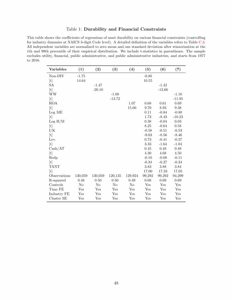
Table 1: Durability and Financial Constraints

This table shows the coefficients of regressions of asset durability on various financial constraints (controllingfor industry dummies at NAICS 3-digit Code level). A detailed definition of the variables refers to Table C.3.All independent variables are normalized to zero mean and one standard deviation after winsorization at the1th and 99th percentile of their empirical distribution. We include t-statistics in parentheses. The sampleexcludes utility, financial, public administrative, and public administrative industries, and starts from 1977to 2016.

Variables (1) (2) (3) (4) (5) (6) (7)

Non-DIV -1.75 -0.80[t] 14.64 10.55SA -1.47 -1.42[t] -20.10 -13.66WW -1.08 -1.10[t] -13.72 -11.95ROA 1.07 0.68 0.61 0.69[t] 15.00 9.70 8.93 9.38Log ME 0.11 -0.84 -0.80[t] 1.73 -8.43 -10.23Log B/M 0.38 -0.04 0.03[t] 8.25 -0.64 0.58I/K -0.58 -0.51 -0.53[t] -9.03 -8.56 -8.46Lev. 0.73 -0.41 -0.27[t] 3.33 -1.64 -1.04Cash/AT 0.45 0.48 0.48[t] 4.30 4.68 4.50Redp -0.10 -0.08 -0.11[t] -0.34 -0.27 -0.34TANT 3.83 3.88 3.84[t] 17.00 17.33 17.05Observations 130,059 130,059 120,135 129,924 99,292 99,292 94,299R-squared 0.48 0.50 0.50 0.49 0.68 0.69 0.69Controls No No No No Yes Yes YesTime FE Yes Yes Yes Yes Yes Yes YesIndustry FE Yes Yes Yes Yes Yes Yes YesCluster SE Yes Yes Yes Yes Yes Yes Yes

48

Table 2: Summary Statistics

This table presents summary statistics for the main outcome variables and control variables of our sample.The detailed definition of asset durability and depreciation measure refers to Section 2.1 Debt leverage is theratio of long-term debt (DLTT) over the sum of leased capital and total assets (AT), where leased capital isdefined as 10 times rental expense (XRENT). Rental leverage is the ratio of leased capital over the sum ofleased capital and total assets (AT). Leased capital leverage is the sum of debt leverage and rental leverage.In Panel A, we split the whole sample into constrained and unconstrained firms at the end of every June,as classified by dividend payment dummy (DIV), according to Farre-Mensa and Ljungqvist (2016). Wereport pooled means of these variables value-weighted by firm market capitalization at fiscal year end. InPanel B, we report the time-series averages of the cross-sectional median of firm characteristics across fiveportfolios sorted on asset durability relative to their industry peers according to the NAICS 3-digit industryclassifications. The detailed definition of the variables is listed in Appendix C. The sample is 1977 to 2016and excludes financial, utility, and public administrative from the analysis.

Panel A: Pooled Statistics Panel B: Firm Characteristics

Const. Unconst. Portfolios

Variables Mean L 2 3 4 H

Durability 12.66 16.54 7.69 9.99 11.45 14.24 18.00Depreciation 0.17 0.13 0.19 0.16 0.15 0.13 0.11Book Lev. 0.24 0.33 0.13 0.19 0.21 0.28 0.32

49

Table 3: Portfolios Sorted on Asset Durability

This table shows average excess returns for five portfolios sorted on asset durability across firms relative totheir industry peers, for which we use the NAICS 3-digit industry classifications and rebalance portfolios atthe end of every June. The results reflect monthly data, for which the sample is from July 1978 to December2017 and excludes utility, financial, public administrative, and public administrative industries. We splitthe whole sample into financially constrained and unconstrained subsample at the end of every June, asclassified by dividend payment dummy, SA index, rating dummy, and WW index. We report average excessreturns over the risk-free rate E[R]-Rf, standard deviations Std, and Sharpe ratios SR across five portfolios inconstrained subsamples (Panel A) and in whole sample (Panel B). Standard errors are estimated by using theNewey-West correction. We include t-statistics in parentheses and annualize portfolio returns multiplying by12. All returns, standard deviations, and Sharpe ratios have been annualized.

Panel A: Constrained Subsample

L 2 3 4 H H-L

DIV

E[R]-Rf (%) 5.39 9.57 9.34 9.03 12.32 6.93[t] 1.48 2.81 2.81 2.92 3.62 2.86Std (%) 26.79 25.32 24.81 24.05 24.09 11.80SR 0.20 0.38 0.38 0.38 0.51 0.59

SA Index

E[R]-Rf (%) 4.53 7.59 7.97 8.39 9.63 5.10[t] 1.12 1.89 1.98 2.35 2.77 2.54Std (%) 24.45 23.55 24.34 21.09 20.7 11.58SR 0.19 0.32 0.33 0.40 0.47 0.44

Rating

E[R]-Rf (%) 5.65 8.76 9.40 9.35 10.10 4.45[t] 1.42 2.18 3.06 2.84 3.52 2.12Std (%) 24.32 23.4 19.61 19.89 18.81 11.8SR 0.23 0.37 0.48 0.47 0.54 0.38

WW Index

E[R]-Rf (%) 6.09 8.24 9.13 9.59 9.65 3.56[t] 2.13 2.78 3.68 3.78 3.85 2.23Std (%) 25.7 24.18 23.67 21.1 20.85 11.04SR 0.24 0.34 0.39 0.45 0.46 0.32

Panel B: Whole Sample

E[R]-Rf (%) 7.36 8.10 8.12 8.65 8.79 1.44[t] 2.70 3.49 3.26 4.17 3.55 1.03Std (%) 19.25 16.75 15.14 15.15 17.37 8.72SR 0.38 0.48 0.54 0.57 0.51 0.17

50

Table 4: Calibration

We calibrate the model at the quarterly frequency. This table reports the parameter values and thecorresponding moments (annalized) we used in the calibration procedure.

Parameter Symbol Value

Relative risk aversion γ 10IES ψ 2Capital share α 0.30Span of control parameter ν 0.90

Mean productivity growth rate E(A) 0.1248Time discount factor β 0.99Durable capital dep. rate δd 0.01Non-durable capital dep. rate δnd 0.03Death rate of entrepreneurs E(λ) 0.025Collateralizability parameter θ 0.33Transfer to entering entrepreneurs χ 0.89

Persistence of TFP shock ρA 0.994Persistence of λ shock ρx 0.98Vol. of λ shock σx 0.05Vol. of productivity shock σA 0.00695Inv. adj. cost parameter ζ 25

Mean idio. productivity growth µZ 0.005Vol. of idio. productivity growth σZ 0.025

51

Table 5: Model Simulations and Aggregate Moments

This table presents the moments from the model simulation. The market return RM corresponds to the

return on entrepreneurs’ net worth and embodies an endogenous financial leverage. RLevd , RLev

nd denotes

the levered capital returns, by the average financial leverage in the economy. We simulate the economy at

monthly frequency, then aggregate the monthly observations to annual frequency. The moments reported are

based on the annual observations. Number in parenthesis are standard errors of the calculated moments.

Moments Data Model

σ(∆y) 3.05 (0.60) 3.32σ(∆c) 2.53 (0.56) 2.88σ(∆i) 10.30 (2.36) 6.15corr(∆c,∆i) 0.39(0.29) 0.77AC1(∆c) 0.49(0.15) 0.45

E[RM −Rf ] 5.71 (2.25) 6.82σ(RM −Rf ) 20.89 (2.21) 16.04E[Rf ] 1.10 (0.16) 1.15σ(Rf ) 0.97 (0.31) 0.80E[RLevd −Rf ] 5.50E[RLevnd −Rf ] 1.50

52

Table 6: Asset Durability Spread, Data, and Model Comparison

This table compares the moments in the empirical data (Panel A) and the model simulated data (Panel B) atthe portfolio level. Panel A reports the statistics computed from the sample of financially constrained firmsin the data, as classified by dividend payment dummy (DIV). In Panel B, we implement model simulationand then perform the same portfolio sorts as in the data. Panel A and B show the time series average of thecross-sectional median of firm characteristics using the value from the year end, including asset durability,depreciation rate, book leverage, return on equity. We also report the value-weighted excess returns E[R]-Rf(%) (annualized by multiplying by 12, in percentage terms), for quintile portfolios sorted on asset durability.The detailed definition of the variables is listed in Appendix C. The sample is from July 1978 to December2017 and excludes financial, utility, and public administrative industries from the analysis.

Variables L 2 3 4 H H-L

Panel A: Data

Asset Durability 7.69 9.99 11.45 14.24 18.00Depreciation 0.19 0.16 0.15 0.13 0.11Book Lev. 0.13 0.19 0.21 0.28 0.32ROE 0.12 0.17 0.18 0.22 0.23E[R]-Rf (%) 5.39 9.57 9.34 9.03 12.32 6.93

Panel B: Model

Asset Durability 8.33 10.05 11.12 14.28 20.08Depreciation 0.12 0.10 0.09 0.07 0.05Book Lev. 0.19 0.27 0.33 0.39 0.45ROE 0.06 0.08 0.09 0.11 0.13E[R]-Rf (%) 3.39 5.27 5.96 6.60 7.02 3.63

53

Table 7: Aggregate Shocks and Price Dynamics

This table shows the exposure of price dynamics to aggregate macroeconomic shocks. All estimates are basedon the following panel regressions:

∆qh,t = βy ∆yt + βd Asset Durabilityh,t ×∆yt + εh,t,

in which ∆qh,t denotes price dynamics of asset h, ∆yt denotes aggregate macroeconomic shocks, andAsset Durabilityh denotes the asset durability of asset h at year t. We control for asset fixed effects, andstandard errors are clustered at the asset level. We report t-statistics in parenthesis. The sample period isfrom 1977 to 2017.

(1) (2)

dy 1.51 1.02[t] 11.71 3.89Interaction 1.06[t] 3.28

Observations 4,830 4,760Asset FE Yes YesCluster SE Yes Yes

54

Table 8: Asset Pricing Factor Tests

This table shows asset pricing test for five portfolios sorted on asset durability across firms relative to theirindustry peers, where we use the NAICS 3-digit industry classifications and rebalance portfolios at the end ofevery June. The results reflect monthly data, for which the sample is from July 1978 to December 2017 andexcludes utility, financial, and public administrative industries. We split the whole sample into financiallyconstrained and unconstrained firms, as classified by the dividend payment dummy (DIV), and report fiveportfolios across the financially constrained subsample. In Panel A, we report the portfolio alphas andbetas by the Fama-French five-factor model plus the long-short portfolio sorted on collateralizability (COL),including MKT, SMB, HML, RMW, CMA, and LMH. In panel B, we report portfolio alphas and betas bythe HXZ q-factor model plus the long-short portfolio sorted on collateralizability, including MKT, SMB, I/A,ROE, and COL. Data on the Fama-French five-factor model are from Kenneth French’s website. Data onthe I/A and ROE factor are provided by Kewei Hou, Chen Xue, and Lu Zhang. Data on the long-shortportfolio sorted on collateralizability refers to Ai, Li, Li, and Schlag (2019). Standard errors are estimatedusing Newey-West correction. We include t-statistics in parentheses and annualize the portfolio alphas bymultiplying 12.

L 2 3 4 H H-L

Panel A: FF5 + LMH

αFF5+COL -4.13 2.51 1.55 0.43 4.02 8.14[t] -2.06 1.44 0.94 0.29 2.52 3.38MKT 1.28 1.14 1.15 1.13 1.17 -0.11[t] 24.57 32.69 29.01 36.65 33.10 -2.22SMB 0.51 0.46 0.36 0.46 0.43 -0.08[t] 5.97 6.35 6.22 8.25 7.54 -0.91HML -0.24 -0.35 -0.33 -0.46 -0.38 -0.15[t] -2.45 -4.77 -4.35 -6.83 -4.92 -1.69RMW -0.10 -0.24 -0.11 0.02 -0.06 0.04[t] -0.78 -2.19 -1.53 0.34 -0.78 0.25CMA -0.44 -0.42 -0.51 -0.31 -0.25 0.19[t] -3.21 -4.18 -4.58 -3.27 -2.88 1.47COL 0.10 0.13 0.13 0.09 0.03 -0.07[t] 2.67 3.50 3.69 2.88 0.83 -1.67

Panel B: HXZ + LMH

αHXZ+COL -4.71 1.65 1.60 -0.30 3.82 8.54[t] -2.36 0.86 0.79 -0.17 2.26 3.48MKT 1.31 1.18 1.17 1.15 1.18 -0.13[t] 19.40 28.08 26.40 28.47 30.62 -2.20SMB 0.42 0.37 0.26 0.37 0.37 -0.06[t] 3.30 3.96 4.37 5.74 7.01 -0.42I/A -0.62 -0.77 -0.88 -0.80 -0.69 -0.08[t] -5.18 -8.05 -9.03 -9.30 -8.59 -0.64ROE -0.03 -0.08 -0.04 0.12 0.01 0.04[t] -0.34 -0.98 -0.55 1.92 0.17 0.62COL 0.17 0.24 0.21 0.18 0.11 -0.06[t] 3.36 6.21 6.36 6.13 3.83 -1.15

55

Table 9: Fama-Macbeth Regressions

This table reports the of Fama-Macbeth regressions of individual stock excess returns on their asset durabilityand other firm characteristics. The sample is from July 1978 to December 2017 and excludes financial, utility,and public administrative industries from the analysis. We split the whole sample into financially constrainedand unconstrained firms, as classified by the dividend payment dummy, and then report the result of regressionin the financially constrained subsample. For each month from July of year t to June of year t+1, we regressmonthly excess returns of individual stock on durability with different sets of variables that are known by theend of June of year t, and control for industry fixed effects based on NAIC 3-digit industry classifications.We present the time-series average and heteroscedasticity-robust t-statistics of the slopes (i.e., coefficients)estimated from the monthly cross-sectional regressions for different model specifications. All independentvariables are normalized to zero mean and one standard deviation after winsorization at the 1th and 99thpercentile of their empirical distribution. We include t-statistics in parentheses and annualize individualstock excess returns by multiplying 12. Standard errors are estimated using Newey-West correction.

Variables (1) (2) (3)

Asset Durability 2.13 3.62 1.46[t] 3.44 5.24 2.86Book Lev. -1.89 -0.57 -0.99[t] -4.17 -1.09 -2.28Collateralizability -3.07[t] -3.87Log ME -0.75[t] -0.67Log B/M 4.82[t] 8.73ROA 6.36[t] 8.98I/K -1.13[t] -2.78OC/AT 1.03[t] 2.29R&D/AT 5.71[t] 7.05

Observations 846,277 632,464 806,449Controls No No YesIndustry FE Yes Yes Yes

56

Table 10: Cash Flow Sensitivity

This table shows the cash flow sensitivity of the asset durability-sorted portfolios to the TFP and GDP shock.Panel A and B report sensitivities from empirical data and model simulated data, respectively. The portfolio-level normalized cash flow is constructed by aggregating cash flow (EBIT) within each quintile portfolio, andthen normalized by the lagged aggregate sales (SALE) of the given portfolio. We regress portfolio-levelnormalized cash flow on TFP and wealth share shock, respectively, and then report estimated coefficients onnormalized cash flow. Standard errors are estimated by Newey-West correction, and t-statistics are includedin parentheses. All regressions are conducted at the annual frequency. The sample includes annual data from1979 to 2017.

L 2 3 4 H H-L

TFP 1.16 1.29 1.63 1.58 1.78 0.62[t] 14.95 8.88 17.82 10.30 9.06 4.25GDP 1.33 2.01 2.10 2.08 2.54 1.21[t] 3.76 5.79 4.49 4.72 4.60 5.59

57

Table 11: Estimating the Market Price of Risk

This table shows results the GMM estimates of the stochastic discount factor’s parameters. In Panel A,we use the asset durability-sorted portfolios as test portfolios and report risk exposures with respect to themeasures of aggregate macroeconomic shock. We use two sets of proxies for the aggregate macroeconomicshock (Macro): the the log difference in TFP and GDP. In Panel B, we present GMM estimates of theparameters of the stochastic discount factor M = 1 − bMMKT − bA ×Macro, using the leased capital ratiosorted portfolios. We do the normalization such that E[M ] = 1 (See, e.g., Cochrane (2005)). We report HACt-statistics computed errors using the Newey-West procedure adjusted for three lags. As a measure of fit, wereport the sum of squared errors (SSQE), mean absolute pricing errors (MAPE), and the J-statistic of theoveridentifying restrictions of the model. The sample includes annual data from 1979 to 2017.

Panel A: Portfolio Risk Exposures

L 2 3 4 H H-L

TFP 0.36 1.92 1.37 1.48 2.33 1.89[t] 0.75 1.93 1.34 1.73 2.16 2.15GDP -0.09 2.97 1.63 1.48 3.32 3.37[t] -0.03 0.83 0.51 0.37 0.75 1.85

Panel B: Price of Risks

Parameters CAPM TFP GDP

bM 0.02 0.01 0.01[t] 3.66 1.84 1.17bA 0.24 0.70[t] 7.78 4.95

SSEQ (%) 0.78 0.10 0.39MAPE (%) 2.72 1.17 2.30J-test 6.69 3.13 3.40p 0.24 0.53 0.49

58

Appendix A: Proof of Proposition 1

We prove Proposition 1 in two steps: first, given prices, the quantities satisfy the house-

hold’s and the entrepreneurs’ optimality conditions; second, the quantities satisfy the market

clearing conditions.

To verify the optimality conditions, note that the optimization problems of households

and firms are all standard convex programming problems; therefore, we only need to verify

first order conditions. Equation (28) is the household’s first-order condition. Equation (34)

is a normalized version of resource constraint (15). Both of them are satisfied as listed in

Proposition 1.

To verify that the entrepreneur i’s allocations {Ni,t, Bi,t, Kdi,t, K

ndi,t , Li,t} as constructed in

Proposition 1 satisfy the first order conditions for the optimization problem in equation (8),

note that the first order condition with respect to Bi,t implies

µit = Et

[Mt+1

]Rft + ηit. (A1)

Similarly, the first order condition for type-d capital Kdi,t+1 is

µit = Et

[M i

t+1

ΠKd

(At+1, zi,t+1, K

di,t+1, K

ndi,t+1

)+ (1− δd) qd,t+1

qd,t

]+ θηit. (A2)

Finally, the optimality with respect to the choice of type-nd capital Kndi,t+1 implies

µit = Et

[M i

t+1

ΠKnd

(At+1, zi,t+1, K

di,t+1, K

ndi,t+1

)+ (1− δnd) qnd,t+1

qd,t

]+ θηit. (A3)

Next, the law of motion of the endogenous state variable n can be constructed from

equation (9):

n′ = (1− λ)

[ανA′ + ζ (1− δd) qd (A′, n′) + (1− ζ) (1− δnd) qnd (A′, n′)

−θ [ζqd (A, n) + (1− ζ) qnd (A, n)]Rf (A, n)

]+λχ

n

Γ (A, n). (A4)

With the law of motion of the state variables, we can construct the normalized utility of the

59

household as the fixed point of

u (A, n) =

{(1− β)c (A, n)1− 1

ψ + βΓ (A, n)1− 1ψ (E[u (A′, n′)

1−γ])

1− 1ψ

1−γ

} 1

1− 1ψ

.

The stochastic discount factors must be consistent with household utility maximization:

M ′ = β

[c (A′, n′) Γ (A, n)

c (A, n)

]− 1ψ

u (A′, n′)

E[u (A′, n′)1−γ] 1

1−γ

1ψ−γ

(A5)

M ′ = M ′[(1− λ)µ (A′, n′) + λ]. (A6)

In our setup, thanks to the assumptions that the idiosyncratic shock zi,t+1 is observed be-

fore the decisions on Kdi,t+1 and Knd

i,t+1 are made, we can construct an equilibrium in which

µit and ηit are equalized across all the firms because ∂∂Kd

i,t+1Π(At+1, zi,t+1, K

di,t+1, K

ndi,t+1

)=

∂∂Knd

i,t+1Π(At+1, zi,t+1, K

di,t+1, K

ndi,t+1

)are the same for all i.

Our next step is to verify the market clearing conditions. Given the initial conditions

(initial net worth N0,Kd

1

Knd1

= ζ1−ζ , Ni,0 = zi,1N0) and the net worth injection rule for the new

entrant firms (N entrantt+1 = χNt for all t), we establish the market clearing conditions through

the following lemma. For simplicity, we assume the collateral constraint to be binding. The

case in which this constraint is not binding can be dealt with in a similar way.

Lemma 1. The optimal allocations {Ni,t, Bi,t, Kdi,t+1, K

ndi,t+1} constructed as in Proposition 1

satisfy the market clearing conditions, i.e.,

Kdt+1 =

∫Kdi,t+1 di, Knd

t+1 =

∫Kndi,t+1 di, Nt =

∫Ni,t di (A7)

for all t ≥ 0.

First, in each period t, given prices and Ni,t, the individual entrepreneur i’s capital deci-

sions {Kdi,t+1, K

ndi,t+1} must satisfy the condition

Ni,t = [1− θ] qd,tKdi,t+1 + [1− θ] qnd,tKnd

i,t+1 (A8)

and the optimal decision rule (19). Equation (A8) is obtained by combining the entrepreneur’s

budget constraint (4) with a binding collateral constraint (5).

Next, we show by induction, that, given the initial conditions, market clearing conditions

(A7) hold for all t ≥ 0. In period 0, we start from the initial conditions. First, Ni,0 = zi,1N0,

where zi,1 is chosen from the stationary distribution of z. Then, given zi,1 for each firm

60

i, we use equations (A8) and (19) to solve for Kdi,1 and Knd

i,1 . Clearly, Kdi,1 = zi,1K

d1 and

Kndi,1 = zi,1K

nd1 . Therefore, the market clearing conditions (A7) hold for t = 0, i.e.,∫

Kdi,1 di = Kd

1 ,

∫Kndi,1 di = Knd

1 ,

∫Ni,0 di = N0. (A9)

To complete the induction argument, we need to show that if market clearing holds for t+ 1,

it must hold for t+ 2 for all t, which is the following claim:

Claim 1. Suppose∫Kdi,t+1 di = Kd

t+1,∫Kndi,t+1 di = Knd

t+1 ,∫Ni,t di = Nt, and N entrant

t+1 =

χNt, then ∫Kdi,t+2 di = Kd

t+2

∫Kndi,t+2 di = Knd

t+2

∫Ni,t+1 di = Nt+1 (A10)

for all t ≥ 0.

1. Using the law of motion for the net worth of existing firms, one can show that the total

net worth of all surviving firms can be rewritten as follows:

(1− λ)

∫Ni,t+1 di

= (1− λ)

∫ [At+1

(Kdi,t+1 +Knd

i,t+1

)+ (1− δd) qd,t+1K

di,t+1

+ (1− δnd) qnd,t+1Kndi,t+1 −Rf,tBi,t

]di,

= (1− λ)[At+1

(Kdt+1 +Knd

t+1

)+ (1− δd) qd,tKd

t+1 + (1− δnd) qnd,tKndt+1 −Rf,tBt

],

since by assumption∫Kdi,t+1 di = Kd

t+1,∫Kndi,t+1 di = Knd

t+1 , and∫Bi,t di = Bt =

θ[qd,tK

dt+1 + qnd,tK

ndt+1

]. Using the assignment rule for the net worth of new entrants,

N entrantt+1 = χNt, we can show that the total net worth at the end of period t+ 1 across

survivors and new entrants together satisfies∫Ni,t+1 di = Nt+1, where aggregate net

worth Nt+1 is given by equation (9).

2. At the end of period t+1, we have a pool of firms consisting of old ones with net worth

given by (7) and new entrants. All of them will observe zi,t+2 (for the new entrants

zi,t+2 = z) and produce at the beginning of the period t+ 1.

We compute the capital holdings for period t + 2 for each firm i using (A8) and (19).

At this point, the capital holdings and the net worth of all existing firms will not

be proportional to zi,t+2 due to heterogeneity in the shocks. However, we know that∫Ni,t+1 di = Nt+1, and

∫zi,t+2 di = 1. Integrating (A8) and (19) across all i yields the

two equations

Nt+1 = [1− θ] qd,t+1

∫Kdi,t+2 di+ [1− θ] qnd,t+1

∫Kndi,t+2 di (A11)

61

Kdt+2 +Knd

t+2 =

∫Kdi,t+2 di+

∫Kndi,t+2 di, (A12)

where we have used∫Ni,t+1 di = Nt+1 and

∫zi,t+2 di = 1. Given that the constraints

of all entrepreneurs are binding, the budget constraint (A8) also holds at the aggregate

level, i.e.,

Nt+1 = [1− θ] qd,t+1Kdt+2 + [1− θ] qnd,t+1K

ndt+2.

Together with the above system, this implies∫Kdi,t+2 di = Kd

t+2 and∫Kndi,t+2 di = Knd

t+2.

Therefore, the claim is proved.

In summary, we have proved that the equilibrium prices and quantities constructed in

Proposition 1 satisfy the household’s and entrepreneur’s optimality conditions, and that the

quantities satisfy market clearing conditions.

Finally, we provide a recursive relationship that can be used to solve for θ (A, n) given

the equilibrium constructed in Proposition 1. The recursion (8) implies

µtNi,t + θtzi,t+1

(Kdt +Knd

t

)= EtMt+1

[(1− λ)

(µt+1Ni,t+1 + θt+1

(Kdt+1 +Knd

t+1

)zi,t+2

)+ λNi,t+1

],

= EtMt+1

[{(1− λ)µt+1 + λ

}Ni,t+1

]+ (1− λ) zi,t+1Et

[Mt+1θt+1

(Kdt+1 +Knd

t+1

)]. (A13)

Below, we first focus on simplifying the term EtMt+1

[{(1− λ)µt+1 + λ

}Ni,t+1

]. Note that

a binding collateral constraint together with the entrepreneur’s budget constraint (4) implies

[1− θ] qd,tKdi,t+1 + [1− θ] qnd,tKnd

i,t+1 = Ni,t. (A14)

Equation (A14) together with the optimality condition (19) determine Kdi,t+1 and Knd

i,t+1 as

functions of Ni,t and zi,t+1:

Kdi,t+1 =

[1− θ] qnd,tzi,t+1

(Kdt+1 +Knd

t+1

)−Ni,t

[1− θ] qnd,t − [1− θ] qd,t,

Kndi,t+1 =

Ni,t − [1− θ] qd,tzi,t+1

(Kdt+1 +Knd

t+1

)[1− θ] qnd,t − [1− θ] qd,t

. (A15)

Using Equation (A15) and the law of motion of net worth (9), we can represent Ni,t+1 as a

62

linear function of Ni,t and zi,t+1:

Ni,t+1 = zi,t+1αAt+1

(Kdt+1 +Knd

t+1

)+ (1− δd) qd,t+1

(1− θ) qnd,tzi,t+1

(Kdt+1 +Knd

t+1

)−Ni,t

(1− θ) (qnd,t − qd,t)

+ (1− δnd) qnd,t+1

Ni,t − (1− θ) qd,tzi,t+1

(Kdt+1 +Knd

t+1

)(1− θ) (qnd,t − qd,t)

−Rf,tθ (1− δd) qd,t(1− θ) qnd,tzi,t+1

(Kdt+1 +Knd

t+1

)−Ni,t

(1− θ) (qnd,t − qd,t)

−Rf,tθ (1− δnd) qnd,tNi,t − (1− θ) qd,tzi,t+1

(Kdt+1 +Knd

t+1

)(1− θ) (qnd,t − qd,t)

.

Because we are only interested in the coefficients on zi,t+1, collecting the terms that involves

zi,t+1 on both sides of (A13), we have:

θtzi,t+1

(Kdt+1 +Knd

t+1

)= zi,t+1

(Kdt+1 +Knd

t+1

)× Term,

where

Term = Et

Mt+1

αAt+1 + (1− δd)qd,t+1

qnd,tqnd,t−qd,t

+(1− δnd)qnd,t+1−qd,t

qnd,t−qd,t

−Rf,tθqd,tqnd,t

qnd,t−qd,t

−Rf,tθqnd,t−qd,t

qnd,t−qd,t

+ (1− λ)Et [Mt+1θt+1] .

We can simplify the first term using the first order conditions (29)-(31) to get

Et

[Mt+1 {α (1− ν)At+1}

].

Therefore, we have the following recursive relationship for θ (A, n):

θ (A, n) = [1− δ + i (A, n)] {α (1− ν)E [M ′ {λ+ (1− λ)µ (A′, n′)}A′] + (1− λ)E [M ′θ (A′, n′)]} .(A16)

The term α (1− ν)A′ is the profit for the firm due to decreasing return to scale. Clearly,

θ (A, n) has the interpretation of the present value of profit. In the case of constant returns

to scale, θ (A, n) = 0.

63

Appendix B: Data Construction

This section describes how we (i) construct firm samples for empirical analysis and (ii) con-

struct firm characteristics to control for fundamentals.

B.1. Asset Prices and Accounting Data

Our sample consists of firms in the intersection of Compustat and CRSP (Center for Research

in Security Prices). We obtain accounting data from Compustat and stock returns data from

CRSP. Our sample firms include those with positive durability data and non-missing SIC

codes and those with domestic common shares (SHRCD = 10 and 11) trading on NYSE,

AMEX, and NASDAQ, except utility firms that have four-digit standard industrial classifi-

cation (SIC) codes between 4900 and 4999, finance firms that have SIC codes between 6000

and 6999 (finance, insurance, trusts, and real estate sectors), and public administrative firms

that have SIC codes between 9000 and 9999. We follow Campello and Giambona (2013) by

excluding firm-year observations for which the value of total assets or sales is less than $ 1

million. Following Fama and French (1993), we further drop closed-end funds, trusts, Amer-

ican Depository Receipts, Real Estate Investment Trusts, and units of beneficial interest.

To mitigate backfilling bias, firms in our sample must be listed on Compustat for two years

before including them in our sample. Macroeconomic data are from the Federal Reserve

Economic Data (FRED) maintained by Federal Reserve in St. Louis.

Appendix C: Additional Empirical Evidence

In this section, we provide additional empirical evidence on the relation of the asset durability

and other firm characteristics and document the summary statistics of the asset durability

across industries.

C.1. More Detailed Firm Characteristics

Table C.1 documents how differences in asset durability among firms are related to other firm

characteristics. We report average durability and these characteristics across five portfolios

sorted on the firm-level asset durability among financially constrained firms

[Place Table C.1 about here]

64

Generally speaking, our sample contains 1, 821 firms. Five portfolios sorted on asset

durability from the lowest to the highest quintile are evenly distributed, with the average

number of firms ranging from 301 to 417. The cross-sectional variations in durability are

large, ranging from 7.69 to 18 across five portfolios sorted on durability. Size does not vary a

lot but presents a hump-shaped pattern across five portfolios. Moreover, a firm with a lower

asset durability has a lower book-to-market ratio (B/M) and a higher investment rate (I/K)

and Tobin’s q to reflect more investment opportunities. We also notice that low durability

firms are less profitable, as measure of return on assets (ROA), and lower capacity to borrow,

as measure by book leverage, and more financially constrained (SA and WW index). These

characteristics suggest an endogenous choice for less durable assets when a firm becomes

more financially constrained with low tangibility but faces a positive investment opportunity.

Finally, there is a negative relationship between asset durability and collateralizability.

C.2. Summary Statistics across Industries

In Table C.2, we report the average of asset durability and depreciation with respect to

tangible and intangible assets in each industry according to the BEA industry classifications.

Asset durability (depreciation) in some industries are higher (lower), such as the educational

services and the accommodation industry. There are comparatively large cross-industry

variations in asset durability (depreciation), ranging from 10.84 to 49.49 . Therefore, to

make sure our results are not driven by any particular industry, we control for industry

effects as detailed later.

[Place Table C.2 about here]

65

Table C.1: Firm Characteristics

This table reports time-series averages of the cross-sectional median of firm characteristics in five portfoliossorted on asset durability, relative to their industry peers, where we use the NAICS 3-digit classifications andrebalance portfolios at the end of every June. The sample is from 1977 to 2016 and excludes financial, utility,and public administrative industries from the analysis. We split the whole sample into financially constrainedand unconstrained firms at the end of every June, as classified by dividend payment dummy (DIV) accordingto Farre-Mensa and Ljungqvist (2016), and report five portfolios across the financially constrained subsample.The detailed definition of the variables is listed in C.3.

Variables L 2 3 4 H

Asset Durability 7.69 9.99 11.45 14.24 18.00Depreciation 0.19 0.16 0.15 0.13 0.11Log ME 4.88 5.13 5.16 5.22 5.07B/M 0.48 0.51 0.53 0.60 0.67I/K 0.37 0.30 0.28 0.24 0.22q 1.65 1.54 1.48 1.37 1.27ROA 0.07 0.09 0.10 0.11 0.11ROE 0.12 0.17 0.18 0.22 0.23OC/AT 0.36 0.25 0.21 0.17 0.13R&D/AT 0.03 0.03 0.03 0.00 0.00Collateralizability 0.21 0.25 0.27 0.37 0.51Book Lev. 0.13 0.19 0.21 0.28 0.32Short-term Lev. 0.02 0.02 0.02 0.03 0.03Long-term Lev. 0.04 0.09 0.11 0.17 0.21TANT 0.08 0.13 0.17 0.25 0.34SA -2.47 -2.68 -2.80 -2.91 -2.92WW -0.16 -0.18 -0.19 -0.20 -0.20Cash Flow Duration 20.43 20.15 19.99 19.47 18.96Number of Firms 365 345 301 393 417

66

Table C.2: Asset Durability and Depreciation across BEA Industries

This table reports summary statistics of the average asset durability and depreciation with respect to tangibleand intangible assets across industries. Industries are based on BEA industry classifications. The sampleperiod is 1977 to 2016.

BEA Industries Tangible Intangible

Industry Name Durability Depreciation Durability Depreciation

Farms 27.92 0.07 2.58 0.40Forestry, fishing, and related activities 24.43 0.09 2.38 0.43Oil and gas extraction 14.98 0.07 4.33 0.23Mining, except oil and gas 20.56 0.07 4.50 0.23Support activities for mining 13.67 0.09 3.40 0.30Utilities 40.49 0.03 3.38 0.31Construction 20.13 0.10 3.95 0.26Wood products 22.67 0.07 4.61 0.23Nonmetallic mineral products 20.65 0.07 5.90 0.17Primary metals 21.28 0.07 5.73 0.17Fabricated metal products 19.36 0.08 5.68 0.18Machinery 20.94 0.07 5.68 0.18Computer and electronic products 22.97 0.07 3.44 0.29Electrical equipment, appliances, and components 23.98 0.06 5.89 0.17Motor vehicles, bodies and trailers, and parts 17.97 0.08 3.19 0.31Other transportation equipment 24.09 0.06 4.47 0.22Furniture and related products 23.05 0.06 5.37 0.19Miscellaneous manufacturing 22.33 0.07 5.86 0.17Food, beverage, and tobacco products 21.90 0.07 5.55 0.18Textile mills and textile product mills 22.65 0.06 5.46 0.18Apparel and leather and allied products 26.52 0.06 5.73 0.17Paper products 18.12 0.08 5.38 0.19Printing and related support activities 19.06 0.08 5.02 0.21Petroleum and coal products 21.09 0.07 5.86 0.17Chemical products 22.25 0.07 8.09 0.12Plastics and rubber products 18.44 0.08 5.72 0.18Wholesale trade 24.93 0.08 4.13 0.25Retail trade 33.63 0.05 4.05 0.26Air transportation 19.23 0.07 3.28 0.31Railroad transportation 44.31 0.03 4.30 0.25Water transportation 18.99 0.06 4.08 0.26Truck transportation 11.49 0.14 4.19 0.26Transit and ground passenger transportation 35.17 0.05 3.50 0.30Pipeline transportation 39.5 0.03 3.12 0.32Other transportation and support activities 30.07 0.06 3.50 0.31Warehousing and storage 37.45 0.04 3.88 0.28Publishing industries (including software) 23.51 0.07 6.39 0.16Motion picture and sound recording industries 29.43 0.05 7.86 0.13Broadcasting and telecommunications 34.89 0.04 5.42 0.19Information and data processing services 22.86 0.10 4.50 0.23Federal Reserve banks 34.66 0.05 3.25 0.31Credit intermediation and related activities 26.75 0.07 2.99 0.34Securities, commodity contracts, and investments 35.37 0.04 3.12 0.32Insurance carriers and related activities 33.83 0.05 3.10 0.33Funds, trusts, and other financial vehicles 40.54 0.03 3.02 0.33Real estate 40.04 0.03 2.89 0.35Rental and leasing services and lessors of intangible assets 10.84 0.12 2.87 0.35Legal services 31.14 0.06 2.57 0.40Computer systems design and related services 31.76 0.07 2.83 0.35Miscellaneous professional, scientific, and technical services 26.62 0.07 5.41 0.19Management of companies and enterprises 35.71 0.04 3.23 0.31Administrative and support services 29.09 0.07 2.79 0.36Waste management and remediation services 48.14 0.05 3.91 0.26Educational services 49.49 0.03 4.80 0.21Ambulatory health care services 34.39 0.06 4.86 0.21Hospitals 45.77 0.04 4.39 0.24Nursing and residential care facilities 39.67 0.04 5.05 0.20Social assistance 37.26 0.04 3.18 0.32Performing arts, spectator sports, museums, and related activities 36.87 0.04 6.10 0.16Amusements, gambling, and recreation industries 30.35 0.05 3.95 0.26Accommodation 48.59 0.03 4.07 0.25Food services and drinking places 27.15 0.07 4.16 0.24Other services, except government 43.02 0.04 5.24 0.19

67

Table C.3: Definition of Variables

Variables Definition Sources

Durability Details refer to Section 2.1 BEA; Compustat

Depreciation Details refer to Section 2.1 BEA; Compustat

ME (real)Market capitalization deflated by CPI at the end ofJune in year t.

CRSP

B/MThe ratio of book equity of fiscal year ending inyear t-1 to market equity at the end of year t-1.

Compustat

Tobin’s qThe sum of market capitalization at the end of yearand book value of preferred shares deductinginventories over total assets (AT).

CRSP; Compustat

I/KThe ratio of investment (CAPX) to purchasedcapital (PPENT).

Compustat

ROAThe ratio of operating income before depreciation(OIBDP) over total assets (AT).

Compustat

ROEThe ratio of operating income before depreciation(OIBDP) over book equity.

Compustat

OC/AT Following Peters and Taylor (2017). Compustat

R&D Intensity Following Peters and Taylor (2017). Compustat

TangibilityThe ratio of purchased capital (PPENT) to totalassets (AT).

Compustat

Book Lev.The sum of long-term liability (DLTT) and currentliability (DLCT) divided by total assets (AT).

Compustat

Short-term Lev.Current liability (DLCT) divided by total assets(AT).

Compustat

Long-term Lev.Long-term liability (DLTT) divided by total assets(AT).

Compustat

DIV Following Farre-Mensa and Ljungqvist (2016). Compustat

SA Index Following Hadlock and Pierce (2010). Compustat

Credit Rating

The entire list of credit ratings is as follows: AA+,AA, and AA- = 6, A+, A, and A- = 5, BBB+,BBB, BBB- = 4, BB+, BB, BB- = 3, B+, B, andB- = 2, rating below B- or missing is 0.

Compustat

WW Index Following Whited and Wu (2006). Compustat

Cash Flow Duration Following Dechow et al. (2004). Compustat

68