The Art ofComputerProgramming

The A

rt of Com

puter P

rogramm

ing V

olum

e 4 Fascicle 6

VOLUME 4

Satisfiability

DonalD E. Knuth

NEWLY AVAILABLE SECTION OF THE CLASSIC WORK

KN

UTH

Computer Science/Programming/Algorithms

informit.com/aw

Text printed on recycled paper

New

$29.99 US | $36.99 CANADA

This multivolume work on the analysis of algorithms has long been recognized as the definitive description of classical computer science. The four volumes published to date already comprise a unique and invaluable resource in programming theory and practice. Countless readers have spoken about the profound personal influence of Knuth’s writings. Scientists have marveled at the beauty and elegance of his analysis, while practicing programmers have successfully applied his “cookbook” solutions to their day-to-day problems. All have admired Knuth for the breadth, clarity, accuracy, and good humor found in his books.

To continue the fourth and later volumes of the set, and to update parts of the existing volumes, Knuth has created a series of small books called fascicles, which are published at regular intervals. Each fascicle encompasses a section or more of wholly new or revised material. Ultimately, the content of these fascicles will be rolled up into the comprehensive, final versions of each volume, and the enormous undertaking that began in 1962 will be complete.

Volume 4 Fascicle 6 This fascicle, brimming with lively examples, forms the middle third of what will eventually become hardcover Volume 4B. It introduces and surveys “Satisfiability,’’ one of the most fundamental problems in all of computer science: Given a Boolean function, can its variables be set to at least one pattern of 0s and 1s that will make the function true?

Satisfiability is far from an abstract exercise in understanding formal systems. Revolutionary methods for solving such problems emerged at the beginning of the twenty-first century, and they’ve led to game-changing applications in industry. These so-called “SAT solvers’’ can now routinely find solutions to practical problems that involve millions of variables and were thought until very recently to be hopelessly difficult.

Fascicle 6 presents full details of seven different SAT solvers, ranging from simple algorithms suitable for small problems to state-of-the-art algorithms of industrial strength. Many other significant topics also arise in the course of the discussion, such as bounded model checking, the theory of traces, Las Vegas algorithms, phase changes in random processes, the efficient encoding of problems into conjunctive normal form, and the exploitation of global and local symmetries. More than 500 exercises are provided, arranged carefully for self-instruction, together with detailed answers.

Donald E. Knuth is known throughout the world for his pioneering work on algorithms and programming techniques, for his invention of the TEX and METAFONT systems for computer typesetting, and for his prolific and influential writing. Professor Emeritus of The Art of Computer Programming at Stanford University, he currently devotes full time to the completion of these fascicles and the seven volumes to which they belong.

Register your product at informit.com/register for convenient access to downloads, updates, and corrections as they become available.

6FASCICLEV 4

F 6

The Art of Computer ProgrammingDONALD E. KNUTH

Knuth_All.indd 9 2/5/16 10:40 AM

THE ART OFCOMPUTER PROGRAMMINGVOLUME 4, FASCICLE 6

Satisfiability

DONALD E. KNUTH Stanford University

677

ADDISON–WESLEYBoston · Columbus · Indianapolis · New York · San FranciscoAmsterdam · Cape Town · Dubai · London · Madrid · MilanMunich · Paris · Montréal · Toronto · Mexico City · Saõ PauloDelhi · Sydney · Hong Kong · Seoul · Singapore · Taipei · Tokyo

The author and publisher have taken care in the preparation of this book,but make no expressed or implied warranty of any kind and assume noresponsibility for errors or omissions. No liability is assumed for incidentalor consequential damages in connection with or arising out of the use ofthe information or programs contained herein.For sales outside the U.S., please contact:

International Salesinternational@pearsoned.com

Visit us on the Web: www.informit.com/aw

Library of Congress Cataloging-in-Publication DataKnuth, Donald Ervin, 1938-

The art of computer programming / Donald Ervin Knuth.viii,310 p. 24 cm.Includes bibliographical references and index.Contents: v. 4, fascicle 6. Satisfiability.ISBN 978-0-134-39760-3 (pbk. : alk. papers : volume 4, fascicle 6)

1. Computer programming. 2. Computer algorithms. I. Title.QA76.6.K64 2005005.1–dc22

2005041030

Internet page http://www-cs-faculty.stanford.edu/~knuth/taocp.html containscurrent information about this book and related books.See also http://www-cs-faculty.stanford.edu/~knuth/sgb.html for informationabout The Stanford GraphBase, including downloadable software for dealing withthe graphs used in many of the examples in Chapter 7.And see http://www-cs-faculty.stanford.edu/~knuth/mmix.html for basic infor-mation about the MMIX computer.Electronic version by Mathematical Sciences Publishers (MSP), http://msp.orgCopyright c⃝ 2015 by Pearson Education, Inc.All rights reserved. Printed in the United States of America. This publication isprotected by copyright, and permission must be obtained from the publisher prior toany prohibited reproduction, storage in a retrieval system, or transmission in any formor by any means, electronic, mechanical, photocopying, recording, or likewise. Forinformation regarding permissions, write to:

Pearson Education, Inc.Rights and Contracts Department501 Boylston Street, Suite 900Boston, MA 02116

ISBN-13 978-0-13-439760-3ISBN-10 0-13-439760-6

First digital release, February 2016

PREFACE

These unforeseen stoppages,which I own I had no conception of when I first set out;

— but which, I am convinced now, will rather increase than diminish as I advance,— have struck out a hint which I am resolved to follow;

— and that is, — not to be in a hurry;— but to go on leisurely, writing and publishing two volumes of my life every year;

— which, if I am suffered to go on quietly, and can make a tolerable bargainwith my bookseller, I shall continue to do as long as I live.

— LAURENCE STERNE, The Life and Opinions ofTristram Shandy, Gentleman (1759)

This booklet is Fascicle 6 of The Art of Computer Programming, Volume 4:Combinatorial Algorithms. As explained in the preface to Fascicle 1 of Volume 1,I’m circulating the material in this preliminary form because I know that thetask of completing Volume 4 will take many years; I can’t wait for people tobegin reading what I’ve written so far and to provide valuable feedback.

To put the material in context, this lengthy fascicle contains Section 7.2.2.2of a long, long chapter on combinatorial algorithms. Chapter 7 will eventuallyfill at least four volumes (namely Volumes 4A, 4B, 4C, and 4D), assuming thatI’m able to remain healthy. It began in Volume 4A with a short review of graphtheory and a longer discussion of “Zeros and Ones” (Section 7.1); that volumeconcluded with Section 7.2.1, “Generating Basic Combinatorial Patterns,” whichwas the first part of Section 7.2, “Generating All Possibilities.” Volume 4B willresume the story with Section 7.2.2, about backtracking in general; then Section7.2.2.1 will discuss a family of methods called “dancing links,” for updating datastructures while backtracking. That sets the scene for the present section, whichapplies those ideas to the important problem of Boolean satisfiability, aka ‘SAT’.

Wow — Section 7.2.2.2 has turned out to be the longest section, by far, inThe Art of Computer Programming. The SAT problem is evidently a killer app,because it is key to the solution of so many other problems. Consequently I canonly hope that my lengthy treatment does not also kill off my faithful readers!As I wrote this material, one topic always seemed to flow naturally into another,so there was no neat way to break this section up into separate subsections.(And anyway the format of TAOCP doesn’t allow for a Section 7.2.2.2.1.)

I’ve tried to ameliorate the reader’s navigation problem by adding sub-headings at the top of each right-hand page. Furthermore, as in other sections,the exercises appear in an order that roughly parallels the order in which corre-sponding topics are taken up in the text. Numerous cross-references are provided

iii

iv PREFACE

between text, exercises, and illustrations, so that you have a fairly good chance ofkeeping in sync. I’ve also tried to make the index as comprehensive as possible.

Look, for example, at a “random” page — say page 80, which is part ofthe subsection about Monte Carlo algorithms. On that page you’ll see thatexercises 302, 303, 299, and 306 are mentioned. So you can guess that the mainexercises about Monte Carlo algorithms are numbered in the early 300s. (Indeed,exercise 306 deals with the important special case of “Las Vegas algorithms”; andthe next exercises explore a fascinating concept called “reluctant doubling.”) Thisentire section is full of surprises and tie-ins to other aspects of computer science.

Satisfiability is important chiefly because Boolean algebra is so versatile.Almost any problem can be formulated in terms of basic logical operations,and the formulation is particularly simple in a great many cases. Section 7.2.2.2begins with ten typical examples of widely different applications, and closes withdetailed empirical results for a hundred different benchmarks. The great varietyof these problems — all of which are special cases of SAT — is illustrated on pages116 and 117 (which are my favorite pages in this book).

The story of satisfiability is the tale of a triumph of software engineering,blended with rich doses of beautiful mathematics. Thanks to elegant new datastructures and other techniques, modern SAT solvers are able to deal routinelywith practical problems that involve many thousands of variables, although suchproblems were regarded as hopeless just a few years ago.

Section 7.2.2.2 explains how such a miracle occurred, by presenting com-plete details of seven SAT solvers, ranging from the small-footprint methods ofAlgorithms A and B to the state-of-the-art methods in Algorithms W, L, and C.(Well I have to hedge a little: New techniques are continually being discovered,hence SAT technology is ever-growing and the story is ongoing. But I do thinkthat Algorithms W, L, and C compare reasonably well with the best algorithmsof their class that were known in 2010. They’re no longer at the cutting edge,but they still are amazingly good.)

Although this fascicle contains more than 300 pages, I constantly had to“cut, cut, cut,” because a great deal more is known. While writing the materialI found that new and potentially interesting-yet-unexplored topics kept poppingup, more than enough to fill a lifetime. Yet I knew that I must move on. So Ihope that I’ve selected for treatment here a significant fraction of the conceptsthat will prove to be the most important as time passes.

I wrote more than three hundred computer programs while preparing thismaterial, because I find that I don’t understand things unless I try to programthem. Most of those programs were quite short, of course; but several of themare rather substantial, and possibly of interest to others. Therefore I’ve made aselection available by listing some of them on the following webpage:

http://www-cs-faculty.stanford.edu/~knuth/programs.html

You can also download SATexamples.tgz from that page; it’s a collection ofprograms that generate data for all 100 of the benchmark examples discussed inthe text, and many more.

PREFACE v

Special thanks are due to Armin Biere, Randy Bryant, Sam Buss, NiklasEén, Ian Gent, Marijn Heule, Holger Hoos, Svante Janson, Peter Jeavons, DanielKroening, Oliver Kullmann, Massimo Lauria, Wes Pegden, Will Shortz, CarstenSinz, Niklas Sörensson, Udo Wermuth, and Ryan Williams for their detailedcomments on my early attempts at exposition, as well as to dozens and dozensof other correspondents who have contributed crucial corrections. Thanks also toStanford’s Information Systems Laboratory for providing extra computer powerwhen my laptop machine was inadequate.

I happily offer a “finder’s fee” of $2.56 for each error in this draft when it isfirst reported to me, whether that error be typographical, technical, or historical.The same reward holds for items that I forgot to put in the index. And valuablesuggestions for improvements to the text are worth 32/c each. (Furthermore, ifyou find a better solution to an exercise, I’ll actually do my best to give youimmortal glory, by publishing your name in the eventual book:−)

Volume 4B will begin with a special tutorial and review of probabilitytheory, in an unnumbered section entitled “Mathematical Preliminaries Redux.”References to its equations and exercises use the abbreviation ‘MPR’. (Think ofthe word “improvement.”) A preliminary version of that section can be foundonline, via the following compressed PostScript file:

http://www-cs-faculty.stanford.edu/~knuth/fasc5a.ps.gz

The illustrations in this fascicle currently begin with ‘Fig. 33’ and runthrough ‘Fig. 56’. Those numbers will change, eventually, but I won’t knowthe final numbers until fascicle 5 has been completed.

Cross references to yet-unwritten material sometimes appear as ‘00’; thisimpossible value is a placeholder for the actual numbers to be supplied later.

Happy reading!

Stanford, California D. E. K.23 September 2015

vi PREFACE

A note on notation. Several formulas in this booklet use the notation ⟨xyz⟩ forthe median function, which is discussed extensively in Section 7.1.1. Other for-mulas use the notation x .−y for the monus function (aka dot-minus or saturatingsubtraction), which was defined in Section 1.3.1 . Hexadecimal constants arepreceded by a number sign or hash mark: #123 means (123)16.

If you run across other notations that appear strange, please look under theheading ‘Notational conventions’ in the index to the present fascicle, and/or atthe Index to Notations at the end of Volume 4A (it is Appendix B on pages822–827). Volume 4B will, of course, have its own Appendix B some day.

A note on references. References to IEEE Transactions include a letter codefor the type of transactions, in boldface preceding the volume number. Forexample, ‘IEEE Trans. C-35’ means the IEEE Transactions on Computers,volume 35. The IEEE no longer uses these convenient letter codes, but thecodes aren’t too hard to decipher: ‘EC’ once stood for “Electronic Computers,”‘IT’ for “Information Theory,” ‘SE’ for “Software Engineering,” and ‘SP’ for“Signal Processing,” etc.; ‘CAD’ meant “Computer-Aided Design of IntegratedCircuits and Systems.”

Other common abbreviations used in references appear on page x of Vol-ume 1, or in the index below.

PREFACE vii

An external exercise. Here’s an exercise for Section 7.2.2.1 that I plan to puteventually into fascicle 5:00. [20 ] The problem of Langford pairs on 1, 1, . . . , n, n can be represented as anexact cover problem using columns d1, . . . , dn∪s1, . . . , s2n; the rows are di sj sk for1 ≤ i ≤ n and 1 ≤ j < k ≤ 2n and k = i+j+1, meaning “put digit i into slots j and k.”

However, that construction essentially gives us every solution twice, because theleft-right reversal of any solution is also a solution. Modify it so that we get only halfas many solutions; the others will be the reversals of these.

And here’s its cryptic answer (needed in exercise 7.2.2.2–13):00. Omit the rows with i = n− [n even] and j > n/2.

(Other solutions are possible. For example, we could omit the rows with i = 1 andj ≥ n; that would omit n− 1 rows instead of only ⌊n/2⌋. However, the suggested ruleturns out to make the dancing links algorithm run about 10% faster.)

Now I saw, tho’ too late, the Folly ofbeginning a Work before we count the Cost,

and before we judge rightly of our own Strength to go through with it.— DANIEL DEFOE, Robinson Crusoe (1719)

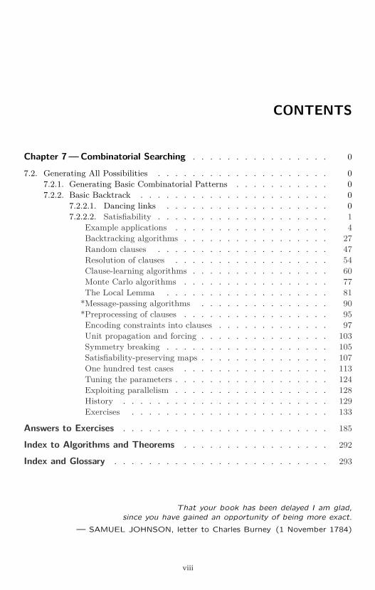
CONTENTS

Chapter 7 — Combinatorial Searching . . . . . . . . . . . . . . . . 0

7.2. Generating All Possibilities . . . . . . . . . . . . . . . . . . . . 07.2.1. Generating Basic Combinatorial Patterns . . . . . . . . . . . 07.2.2. Basic Backtrack . . . . . . . . . . . . . . . . . . . . . . 0

7.2.2.1. Dancing links . . . . . . . . . . . . . . . . . . . 07.2.2.2. Satisfiability . . . . . . . . . . . . . . . . . . . . 1

Example applications . . . . . . . . . . . . . . . . . . 4Backtracking algorithms . . . . . . . . . . . . . . . . . 27Random clauses . . . . . . . . . . . . . . . . . . . . 47Resolution of clauses . . . . . . . . . . . . . . . . . . 54Clause-learning algorithms . . . . . . . . . . . . . . . . 60Monte Carlo algorithms . . . . . . . . . . . . . . . . . 77The Local Lemma . . . . . . . . . . . . . . . . . . . 81

*Message-passing algorithms . . . . . . . . . . . . . . . 90*Preprocessing of clauses . . . . . . . . . . . . . . . . . 95Encoding constraints into clauses . . . . . . . . . . . . . 97Unit propagation and forcing . . . . . . . . . . . . . . . 103Symmetry breaking . . . . . . . . . . . . . . . . . . . 105Satisfiability-preserving maps . . . . . . . . . . . . . . . 107One hundred test cases . . . . . . . . . . . . . . . . . 113Tuning the parameters . . . . . . . . . . . . . . . . . . 124Exploiting parallelism . . . . . . . . . . . . . . . . . . 128History . . . . . . . . . . . . . . . . . . . . . . . . 129Exercises . . . . . . . . . . . . . . . . . . . . . . . 133

Answers to Exercises . . . . . . . . . . . . . . . . . . . . . . . . 185

Index to Algorithms and Theorems . . . . . . . . . . . . . . . . . 292

Index and Glossary . . . . . . . . . . . . . . . . . . . . . . . . . 293

That your book has been delayed I am glad,since you have gained an opportunity of being more exact.

— SAMUEL JOHNSON, letter to Charles Burney (1 November 1784)

viii

7.2.2.2 SATISFIABILITY 1

He reaps no satisfaction but from low and sensual objects,or from the indulgence of malignant passions.

— DAVID HUME, The Sceptic (1742)

I can’t get no . . .

— MICK JAGGER and KEITH RICHARDS, Satisfaction (1965)

7.2.2.2. Satisfiability. We turn now to one of the most fundamental problemsof computer science: Given a Boolean formula F (x1, . . . , xn), expressed in so-called “conjunctive normal form” as an AND of ORs, can we “satisfy” F byassigning values to its variables in such a way that F (x1, . . . , xn) = 1? Forexample, the formula

F (x1, x2, x3) = (x1 ∨ x2) ∧ (x2 ∨ x3) ∧ (x1 ∨ x3) ∧ (x1 ∨ x2 ∨ x3) (1)

is satisfied when x1x2x3 = 001. But if we rule that solution out, by defining

G(x1, x2, x3) = F (x1, x2, x3) ∧ (x1 ∨ x2 ∨ x3), (2)

then G is unsatisfiable: It has no satisfying assignment.Section 7.1.1 discussed the embarrassing fact that nobody has ever been

able to come up with an efficient algorithm to solve the general satisfiabilityproblem, in the sense that the satisfiability of any given formula of size N couldbe decided inNO(1) steps. Indeed, the famous unsolved question “does P = NP?”is equivalent to asking whether such an algorithm exists. We will see in Section7.9 that satisfiability is a natural progenitor of every NP-complete problem.*

On the other hand enormous technical breakthroughs in recent years haveled to amazingly good ways to approach the satisfiability problem. We nowhave algorithms that are much more efficient than anyone had dared to believepossible before the year 2000. These so-called “SAT solvers” are able to handleindustrial-strength problems, involving millions of variables, with relative ease,and they’ve had a profound impact on many areas of research such as computer-aided verification. In this section we shall study the principles that underliemodern SAT-solving procedures.

* At the present time very few people believe that P = NP [see SIGACT News 43, 2 (June2012), 53–77]. In other words, almost everybody who has studied the subject thinks thatsatisfiability cannot be decided in polynomial time. The author of this book, however, suspectsthat NO(1)-step algorithms do exist, yet that they’re unknowable. Almost all polynomial timealgorithms are so complicated that they lie beyond human comprehension, and could never beprogrammed for an actual computer in the real world. Existence is different from embodiment.

2 COMBINATORIAL SEARCHING (F6) 7.2.2.2

To begin, let’s define the problem carefully and simplify the notation, sothat our discussion will be as efficient as the algorithms that we’ll be considering.Throughout this section we shall deal with variables, which are elements of anyconvenient set. Variables are often denoted by x1, x2, x3, . . . , as in (1); but anyother symbols can also be used, like a, b, c, or even d′′′74. We will in fact often usethe numerals 1, 2, 3, . . . to stand for variables; and in many cases we’ll find itconvenient to write just j instead of xj , because it takes less time and less spaceif we don’t have to write so many x’s. Thus ‘2’ and ‘x2’ will mean the samething in many of the discussions below.

A literal is either a variable or the complement of a variable. In other words,if v is a variable, both v and v are literals. If there are n possible variables insome problem, there are 2n possible literals. If l is the literal x2, which is alsowritten 2, then the complement of l, l, is x2, which is also written 2.

The variable that corresponds to a literal l is denoted by |l|; thus we have|v| = |v| = v for every variable v. Sometimes we write ±v for a literal that iseither v or v. We might also denote such a literal by σv, where σ is ±1. Theliteral l is called positive if |l| = l; otherwise |l| = l, and l is said to be negative.

Two literals l and l′ are distinct if l = l′. They are strictly distinct if |l| = |l′|.A set of literals l1, . . . , lk is strictly distinct if |li| = |lj | for 1 ≤ i < j ≤ k.

The satisfiability problem, like all good problems, can be understood in manyequivalent ways, and we will find it convenient to switch from one viewpoint toanother as we deal with different aspects of the problem. Example (1) is an ANDof clauses, where every clause is an OR of literals; but we might as well regardevery clause as simply a set of literals, and a formula as a set of clauses. Withthat simplification, and with ‘xj ’ identical to ‘j’, Eq. (1) becomes

F =1, 2, 2, 3, 1, 3, 1, 2, 3

.

And we needn’t bother to represent the clauses with braces and commas either;we can simply write out the literals of each clause. With that shorthand we’reable to perceive the real essence of (1) and (2):

F = 12, 23, 13, 123, G = F ∪ 123. (3)

Here F is a set of four clauses, and G is a set of five.In this guise, the satisfiability problem is equivalent to a covering problem,

analogous to the exact cover problems that we considered in Section 7.2.2.1: Let

Tn =x1, x1, x2, x2, . . . , xn, xn

= 11, 22, . . . , nn. (4)

“Given a set F = C1, . . . , Cm, where each Ci is a clause and each clauseconsists of literals based on the variables x1, . . . , xn, find a set L of n literalsthat ‘covers’ F ∪Tn, in the sense that every clause contains at least one elementof L.” For example, the set F in (3) is covered by L = 1, 2, 3, and so is the setT3; hence F is satisfiable. The set G is covered by 1, 1, 2 or 1, 1, 3 or · · · or2, 3, 3, but not by any three literals that also cover T3; so G is unsatisfiable.

Similarly, a family F of clauses is satisfiable if and only if it can be coveredby a set L of strictly distinct literals.

7.2.2.2 SATISFIABILITY 3

If F ′ is any formula obtained from F by complementing one or more vari-ables, it’s clear that F ′ is satisfiable if and only if F is satisfiable. For example,if we replace 1 by 1 and 2 by 2 in (3) we obtain

F ′ = 12, 23, 13, 123, G′ = F ′ ∪ 123.

In this case F ′ is trivially satisfiable, because each of its clauses contains apositive literal: Every such formula is satisfied by simply letting L be the set ofpositive literals. Thus the satisfiability problem is the same as the problem ofswitching signs (or “polarities”) so that no all-negative clauses remain.

Another problem equivalent to satisfiability is obtained by going back to theBoolean interpretation in (1) and complementing both sides of the equation. ByDe Morgan’s laws 7.1.1–(11) and (12) we have

F (x1, x2, x3) = (x1 ∧ x2) ∨ (x2 ∧ x3) ∨ (x1 ∧ x3) ∨ (x1 ∧ x2 ∧ x3); (5)

and F is unsatisfiable⇐⇒ F = 0⇐⇒ F = 1⇐⇒ F is a tautology. ConsequentlyF is satisfiable if and only if F is not a tautology: The tautology problem andthe satisfiability problem are essentially the same.*

Since the satisfiability problem is so important, we simply call it SAT. Andinstances of the problem such as (1), in which there are no clauses of lengthgreater than 3, are called 3SAT. In general, kSAT is the satisfiability problemrestricted to instances where no clause has more than k literals.

Clauses of length 1 are called unit clauses, or unary clauses. Binary clauses,similarly, have length 2; then come ternary clauses, quaternary clauses, and soforth. Going the other way, the empty clause, or nullary clause, has length 0 andis denoted by ϵ; it is always unsatisfiable. Short clauses are very important in al-gorithms for SAT, because they are easier to deal with than long clauses. But longclauses aren’t necessarily bad; they’re much easier to satisfy than the short ones.

A slight technicality arises when we consider clause length: The binaryclause (x1 ∨ x2) in (1) is equivalent to the ternary clause (x1 ∨ x1 ∨ x2) as wellas to (x1 ∨ x2 ∨ x2) and to longer clauses such as (x1 ∨ x1 ∨ x1 ∨ x2); so we canregard it as a clause of any length ≥ 2. But when we think of clauses as setsof literals rather than ORs of literals, we usually rule out multisets such as 112or 122 that aren’t sets; in that sense a binary clause is not a special case of aternary clause. On the other hand, every binary clause (x ∨ y) is equivalent totwo ternary clauses, (x ∨ y ∨ z) ∧ (x ∨ y ∨ z), if z is another variable; and everyk-ary clause is equivalent to two (k + 1)-ary clauses. Therefore we can assume,if we like, that kSAT deals only with clauses whose length is exactly k.

A clause is tautological (always satisfied) if it contains both v and v for somevariable v. Tautological clauses can be denoted by ℘ (see exercise 7.1.4–222).They never affect a satisfiability problem; so we usually assume that the clausesinput to a SAT-solving algorithm consist of strictly distinct literals.

When we discussed the 3SAT problem briefly in Section 7.1.1, we took alook at formula 7.1.1–(32), “the shortest interesting formula in 3CNF.” In our

* Strictly speaking, TAUT is coNP-complete, while SAT is NP-complete; see Section 7.9.

4 COMBINATORIAL SEARCHING (F6) 7.2.2.2

new shorthand, it consists of the following eight unsatisfiable clauses:R = 123, 234, 341, 412, 123, 234, 341, 412. (6)

This set makes an excellent little test case, so we will refer to it frequently below.(The letter R reminds us that it is based on R. L. Rivest’s associative block design6.5–(13).) The first seven clauses of R, namely

R′ = 123, 234, 341, 412, 123, 234, 341, (7)also make nice test data; they are satisfied only by choosing the complements ofthe literals in the omitted clause, namely 4, 1, 2. More precisely, the literals4, 1, and 2 are necessary and sufficient to cover R′; we can also include either 3or 3 in the solution. Notice that (6) is symmetric under the cyclic permutation1 → 2 → 3 → 4 → 1 → 2 → 3 → 4 → 1 of literals; thus, omitting any clauseof (6) gives a satisfiability problem equivalent to (7).A simple example. SAT solvers are important because an enormous varietyof problems can readily be formulated Booleanwise as ANDs of ORs. Let’s beginwith a little puzzle that leads to an instructive family of example problems:Find a binary sequence x1 . . . x8 that has no three equally spaced 0s and nothree equally spaced 1s. For example, the sequence 01001011 almost works; butit doesn’t qualify, because x2, x5, and x8 are equally spaced 1s.

If we try to solve this puzzle by backtracking manually through all 8-bitsequences in lexicographic order, we see that x1x2 = 00 forces x3 = 1. Thenx1x2x3x4x5x6x7 = 0010011 leaves us with no choice for x8. A minute or two offurther hand calculation reveals that the puzzle has just six solutions, namely

00110011, 01011010, 01100110, 10011001, 10100101, 11001100. (8)Furthermore it’s easy to see that none of these solutions can be extended to asuitable binary sequence of length 9. We conclude that every binary sequencex1 . . . x9 contains three equally spaced 0s or three equally spaced 1s.

Notice now that the condition x2x5x8 = 111 is the same as the Booleanclause (x2 ∨ x5 ∨ x8), namely 258. Similarly x2x5x8 = 000 is the same as 258.So we have just verified that the following 32 clauses are unsatisfiable:

123, 234, . . . , 789, 135, 246, . . . , 579, 147, 258, 369, 159,123, 234, . . . , 789, 135, 246, . . . , 579, 147, 258, 369, 159. (9)

This result is a special case of a general fact that holds for any given positiveintegers j and k: If n is sufficiently large, every binary sequence x1 . . . xn containseither j equally spaced 0s or k equally spaced 1s. The smallest such n is denotedby W (j, k) in honor of B. L. van der Waerden, who proved an even more generalresult (see exercise 2.3.4.3–6): If n is sufficiently large, and if k0, . . . , kb−1 arepositive integers, every b-ary sequence x1 . . . xn contains ka equally spaced a’sfor some digit a, 0 ≤ a < b. The least such n is W (k0, . . . , kb−1).

Let us accordingly define the following set of clauses when j, k, n > 0:waerden(j, k;n) =

(xi ∨ xi+d ∨ · · · ∨ xi+(j−1)d)

1 ≤ i ≤ n− (j−1)d, d ≥ 1

∪

(xi ∨ xi+d ∨ · · · ∨ xi+(k−1)d) 1 ≤ i ≤ n− (k−1)d, d ≥ 1

. (10)

7.2.2.2 SATISFIABILITY: EXAMPLE APPLICATIONS 5

The 32 clauses in (9) are waerden(3, 3; 9); and in general waerden(j, k;n) is anappealing instance of SAT, satisfiable if and only if n < W (j, k).

It’s obvious that W(1, k) = k and W(2, k) = 2k− [k even]; but when j and kexceed 2 the numbers W(j, k) are quite mysterious. We’ve seen that W (3, 3) = 9,and the following nontrivial values are currently known:

k = 3 4 5 6 7 8 9 10 11 12 13 14 15 16 17 18 19W(3, k) = 9 18 22 32 46 58 77 97 114 135 160 186 218 238 279 312 349W(4, k) = 18 35 55 73 109 146 309 ? ? ? ? ? ? ? ? ? ?

W(5, k) = 22 55 178 206 260 ? ? ? ? ? ? ? ? ? ? ? ?

W(6, k) = 32 73 206 1132 ? ? ? ? ? ? ? ? ? ? ? ? ?

V. Chvátal inaugurated the study ofW(j, k) by computing the values for j+k ≤ 9as well as W(3, 7) [Combinatorial Structures and Their Applications (1970), 31–33]. Most of the large values in this table have been calculated by state-of-the-artSAT solvers [see M. Kouril and J. L. Paul, Experimental Math. 17 (2008), 53–61; M. Kouril, Integers 12 (2012), A46:1–A46:13]. The table entries for j = 3suggest that we might have W(3, k) < k2 when k > 4, but that isn’t true: SATsolvers have also been used to establish the lower bounds

k = 20 21 22 23 24 25 26 27 28 29 30W(3, k) ≥ 389 416 464 516 593 656 727 770 827 868 903

(which might in fact be the true values for this range of k); see T. Ahmed,O. Kullmann, and H. Snevily [Discrete Applied Math. 174 (2014), 27–51].

Notice that the literals in every clause of waerden(j, k;n) have the samesign: They’re either all positive or all negative. Does this “monotonic” propertymake the SAT problem any easier? Unfortunately, no: Exercise 10 proves thatany set of clauses can be converted to an equivalent set of monotonic clauses.Exact covering. The exact cover problems that we solved with “dancing links”in Section 7.2.2.1 can easily be reformulated as instances of SAT and handed offto SAT solvers. For example, let’s look again at Langford pairs, the task ofplacing two 1s, two 2s, . . . , two n’s into 2n slots so that exactly k slots intervenebetween the two appearances of k, for each k. The corresponding exact coverproblem when n = 3 has nine columns and eight rows (see 7.2.2.1–(00)):

d1 s1 s3, d1 s2 s4, d1 s3 s5, d1 s4 s6, d2 s1 s4, d2 s2 s5, d2 s3 s6, d3 s1 s5. (11)The columns are di for 1 ≤ i ≤ 3 and sj for 1 ≤ j ≤ 6; the row ‘di sj sk’ meansthat digit i is placed in slots j and k. Left-right symmetry allows us to omit therow ‘d3 s2 s6’ from this specification.

We want to select rows of (11) so that each column appears just once. Letthe Boolean variable xj mean ‘select row j’, for 1 ≤ j ≤ 8; the problem is thento satisfy the nine constraints

S1(x1, x2, x3, x4) ∧ S1(x5, x6, x7) ∧ S1(x8)∧ S1(x1, x5, x8) ∧ S1(x2, x6) ∧ S1(x1, x3, x7)

∧ S1(x2, x4, x5) ∧ S1(x3, x6, x8) ∧ S1(x4, x7), (12)

6 COMBINATORIAL SEARCHING (F6) 7.2.2.2

one for each column. (Here, as usual, S1(y1, . . . , yp) denotes the symmetricfunction [y1 + · · ·+ yp = 1].) For example, we must have x5 + x6 + x7 = 1,because column d2 appears in rows 5, 6, and 7 of (11).

One of the simplest ways to express the symmetric Boolean function S1 asan AND of ORs is to use 1 +

(p2)

clauses:

S1(y1, . . . , yp) = (y1 ∨ · · · ∨ yp) ∧⋀

1≤j<k≤p

(yj ∨ yk). (13)

“At least one of the y’s is true, but not two.” Then (12) becomes, in shorthand,

1234, 12, 13, 14, 23, 24, 34, 567, 56, 57, 67, 8,158, 15, 18, 58, 26, 26, 137, 13, 17, 37,

245, 24, 25, 45, 368, 36, 38, 68, 47, 47; (14)

we shall call these clauses langford (3). (Notice that only 30 of them are actuallydistinct, because 13 and 24 appear twice.) Exercise 13 defines langford (n); weknow from exercise 7–1 that langford (n) is satisfiable ⇐⇒ nmod 4 = 0 or 3.

The unary clause 8 in (14) tells us immediately that x8 = 1. Then from thebinary clauses 18, 58, 38, 68 we have x1 = x5 = x3 = x6 = 0. The ternary clause137 then implies x7 = 1; finally x4 = 0 (from 47) and x2 = 1 (from 1234). Rows8, 7, and 2 of (11) now give us the desired Langford pairing 3 1 2 1 3 2.

Incidentally, the function S1(y1, y2, y3, y4, y5) can also be expressed as

(y1 ∨ y2 ∨ y3 ∨ y4 ∨ y5) ∧ (y1∨ y2) ∧ (y1∨ y3) ∧ (y1∨ t)∧ (y2∨ y3) ∧ (y2∨ t) ∧ (y3∨ t) ∧ (t∨ y4) ∧ (t∨ y5) ∧ (y4∨ y5),

where t is a new variable. In general, if p gets big, it’s possible to expressS1(y1, . . . , yp) with only 3p−5 clauses instead of

(p2)+1, by using ⌊(p−3)/2⌋ new

variables as explained in exercise 12. When this alternative encoding is used torepresent Langford pairs of order n, we’ll call the resulting clauses langford ′(n).

Do SAT solvers do a better job with the clauses langford (n) or langford ′(n)?Stay tuned: We’ll find out later.

Coloring a graph. The classical problem of coloring a graph with at most dcolors is another rich source of benchmark examples for SAT solvers. If the graphhas n vertices V , we can introduce nd variables vj , for v ∈ V and 1 ≤ j ≤ d,signifying that v has color j; the resulting clauses are quite simple:

(v1 ∨ v2 ∨ · · · ∨ vd) for v ∈ V (“every vertex has at least one color”); (15)(uj ∨ vj) for u−−−v, 1 ≤ j ≤ d (“adjacent vertices have different colors”). (16)

We could also add n(d2)

additional so-called exclusion clauses

(vi ∨ vj) for v ∈V , 1≤ i< j≤ d (“every vertex has at most one color”); (17)

but they’re optional, because vertices with more than one color are harmless.Indeed, if we find a solution with v1 = v2 = 1, we’ll be extra happy, because itgives us two legal ways to color vertex v. (See exercise 14.)

7.2.2.2 SATISFIABILITY: EXAMPLE APPLICATIONS 7

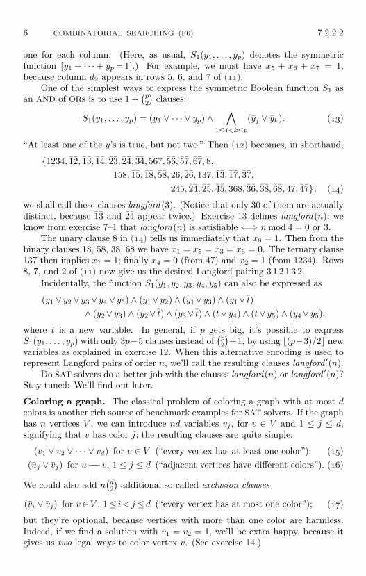
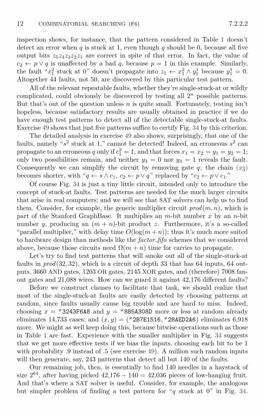
Fig. 33. The McGregor graphof order 10. Each region of this“map” is identified by a two-digit hexadecimal code. Can youcolor the regions with four colors,never using the same color fortwo adjacent regions?

00 01 02 03 04 05 06 07 08 09

11 12 13 14 15 16 17 18 19

22 23 24 25 26 27 28 29

33 34 35 36 37 38 39

44 45 46 47 48 49

55 56 57 58 59

66 67 68 69

77 78 79

88 89

99

20 21

30 31 32

40 41 42 43

50 51 52 53 54

60 61 62 63 64 65

70 71 72 73 74 75 76

80 81 82 83 84 85 86 87

90 91 92 93 94 95 96 97 98

a0 a1 a2 a3 a4 a5 a6 a7 a8 a9

10

Martin Gardner astonished the world in 1975 when he reported [ScientificAmerican 232, 4 (April 1975), 126–130] that a proper coloring of the planarmap in Fig. 33 requires five distinct colors, thereby disproving the longstandingfour-color conjecture. (In that same column he also cited several other “facts”supposedly discovered in 1974: (i) eπ

√163 is an integer; (ii) pawn-to-king-rook-4

(‘h4’) is a winning first move in chess; (iii) the theory of special relativity isfatally flawed; (iv) Leonardo da Vinci invented the flush toilet; and (v) RobertRipoff devised a motor that is powered entirely by psychic energy. Thousandsof readers failed to notice that they had been April Fooled!)

The map in Fig. 33 actually can be 4-colored; you are hereby challenged todiscover a suitable way to do this, before turning to the answer of exercise 18.Indeed, the four-color conjecture became the Four Color Theorem in 1976, asmentioned in Section 7. Fortunately that result was still unknown in April of1975; otherwise this interesting graph would probably never have appeared inprint. McGregor’s graph has 110 vertices (regions) and 324 edges (adjacenciesbetween regions); hence (15) and (16) yield 110 + 1296 = 1406 clauses on 440variables, which a modern SAT solver can polish off quickly.

We can also go much further and solve problems that would be extremelydifficult by hand. For example, we can add constraints to limit the number ofregions that receive a particular color. Randal Bryant exploited this idea in 2010to discover that there’s a four-coloring of Fig. 33 that uses one of the colors only7 times (see exercise 17). His coloring is, in fact, unique, and it leads to anexplicit way to 4-color the McGregor graphs of all orders n ≥ 3 (exercise 18).

Such additional constraints can be generated in many ways. We could,for instance, append

(1108)

clauses, one for every choice of 8 regions, specifyingthat those 8 regions aren’t all colored 1. But no, we’d better scratch that idea:(110

8)

= 409,705,619,895. Even if we restricted ourselves to the 74,792,876,790sets of 8 regions that are independent, we’d be dealing with far too many clauses.

8 COMBINATORIAL SEARCHING (F6) 7.2.2.2

An interesting SAT-oriented way to ensure that x1 + · · · + xn is at most r,which works well when n and r are rather large, was found by C. Sinz [LNCS3709 (2005), 827–831]. His method introduces (n − r)r new variables skj for1 ≤ j ≤ n− r and 1 ≤ k ≤ r. If F is any satisfiability problem and if we add the(n− r − 1)r + (n− r)(r + 1) clauses

(skj ∨ skj+1), for 1 ≤ j < n− r and 1 ≤ k ≤ r, (18)(xj+k ∨ skj ∨ s

k+1j ), for 1 ≤ j ≤ n− r and 0 ≤ k ≤ r, (19)

where skj is omitted when k = 0 and sk+1j is omitted when k = r, then the new set

of clauses is satisfiable if and only ifF is satisfiable with x1+· · ·+xn ≤ r. (See ex-ercise 26.) With this scheme we can limit the number of red-colored regions ofMcGregor’s graph to at most 7 by appending 1538 clauses in 721 new variables.

Another way to achieve the same goal, which turns out to be even better,has been proposed by O. Bailleux and Y. Boufkhad [LNCS 2833 (2003), 108–122]. Their method is a bit more difficult to describe, but still easy to implement:Consider a complete binary tree that has n−1 internal nodes numbered 1 throughn − 1, and n leaves numbered n through 2n − 1; the children of node k, for1 ≤ k < n, are nodes 2k and 2k+1 (see 2.3.4.5–(5)). We form new variables bkj for1 < k < n and 1 ≤ j ≤ tk, where tk is the minimum of r and the number of leavesbelow node k. Then the following clauses, explained in exercise 27, do the job:

(b2ki ∨ b

2k+1j ∨ bki+j), for 0≤ i≤ t2k, 0≤ j≤ t2k+1, 1≤ i+j≤ tk+1, 1<k<n; (20)

(b2i ∨ b3

j ), for 0≤ i≤ t2, 0≤ j≤ t3, i+ j= r + 1. (21)

In these formulas we let tk = 1 and bk1 = xk−n+1 for n ≤ k < 2n; all literals bk0and bkr+1 are to be omitted. Applying (20) and (21) to McGregor’s graph, withn = 110 and r = 7, yields just 1216 new clauses in 399 new variables.

The same ideas apply when we want to ensure that x1 + · · ·+xn is at least r,because of the identity S≥r(x1, . . . , xn) = S≤n−r(x1, . . . , xn). And exercise 30considers the case of equality, when our goal is to make x1 + · · ·+ xn = r. We’lldiscuss other encodings of such cardinality constraints below.

Factoring integers. Next on our agenda is a family of SAT instances with quitea different flavor. Given an (m + n)-bit binary integer z = (zm+n . . . z2z1)2, dothere exist integers x = (xm . . . x1)2 and y = (yn . . . y1)2 such that z = x × y?For example, if m = 2 and n = 3, we want to invert the binary multiplication

y3 y2 y1× x2x1a3 a2 a1

b3 b2 b1c3 c2 c1z5 z4 z3 z2 z1

(a3a2a1)2 = (y3y2y1)2 × x1(b3 b2 b1)2 = (y3y2y1)2 × x2

z1 = a1(c1z2)2 = a2 + b1(c2z3)2 = a3 + b2 + c1(c3z4)2 = b3 + c2

z5 = c3

(22)

when the z bits are given. This problem is satisfiable when z = 21 = (10101)2,in the sense that suitable binary values x1, x2, y1, y2, y3, a1, a2, a3, b1, b2, b3, c1,c2, c3 do satisfy these equations. But it’s unsatisfiable when z = 19 = (10011)2.

7.2.2.2 SATISFIABILITY: EXAMPLE APPLICATIONS 9

Arithmetical calculations like (22) are easily expressed in terms of clausesthat can be fed to a SAT solver: We first specify the computation by constructinga Boolean chain, then we encode each step of the chain in terms of a few clauses.One such chain, if we identify a1 with z1 and c3 with z5, isz1←x1∧y1,

a2←x1∧y2,

a3←x1∧y3,

b1←x2∧y1,

b2←x2∧y2,

b3←x2∧y3,

z2←a2⊕b1,

c1←a2∧b1,

s←a3⊕b2,

p←a3∧b2,

z3←s⊕c1,

q←s∧c1,

c2←p∨q,

z4←b3⊕c2,

z5←b3∧c2,

(23)

using a “full adder” to compute c2z3 and “half adders” to compute c1z2 and c3z4(see 7.1.2–(23) and (24)). And that chain is equivalent to the 49 clauses

(x1∨z1)∧(y1∨z1)∧(x1∨y1∨z1)∧· · ·∧(b3∨c2∨z4)∧(b3∨z5)∧(c2∨z5)∧(b3∨c2∨z5)

obtained by expanding the elementary computations according to simple rules:

t← u ∧ v becomes (u ∨ t) ∧ (v ∨ t) ∧ (u ∨ v ∨ t);t← u ∨ v becomes (u ∨ t) ∧ (v ∨ t) ∧ (u ∨ v ∨ t);t← u⊕ v becomes (u ∨ v ∨ t) ∧ (u ∨ v ∨ t) ∧ (u ∨ v ∨ t) ∧ (u ∨ v ∨ t).

(24)

To complete the specification of this factoring problem when, say, z = (10101)2,we simply append the unary clauses (z5) ∧ (z4) ∧ (z3) ∧ (z2) ∧ (z1).

Logicians have known for a long time that computational steps can readilybe expressed as conjunctions of clauses. Rules such as (24) are now called Tseytinencoding, after Gregory Tseytin (1966). Our representation of a small five-bitfactorization problem in 49+5 clauses may not seem very efficient; but we will seeshortly that m-bit by n-bit factorization corresponds to a satisfiability problemwith fewer than 6mn variables, and fewer than 20mn clauses of length 3 or less.

Even if the system has hundreds or thousands of formulas,it can be put into conjunctive normal form “piece by piece,”

without any “multiplying out.”— MARTIN DAVIS and HILARY PUTNAM (1958)

Suppose m ≤ n. The easiest way to set up Boolean chains for multiplicationis probably to use a scheme that goes back to John Napier’s Rabdologiæ (Edin-burgh, 1617), pages 137–143, as modernized by Luigi Dadda [Alta Frequenza34 (1964), 349–356]: First we form all mn products xi ∧ yj , putting every suchbit into bin [i + j], which is one of m + n “bins” that hold bits to be addedfor a particular power of 2 in the binary number system. The bins will containrespectively (0, 1, 2, . . . , m, m, . . . , m, . . . , 2, 1) bits at this point, with n−m+1occurrences of “m” in the middle. Now we look at bin [k] for k = 2, 3, . . . . Ifbin [k] contains a single bit b, we simply set zk−1 ← b. If it contains two bitsb, b′, we use a half adder to compute zk−1 ← b⊕ b′, c← b∧ b′, and we put thecarry bit c into bin [k + 1]. Otherwise bin [k] contains t ≥ 3 bits; we choose anythree of them, say b, b′, b′′, and remove them from the bin. With a full adder wethen compute r ← b⊕b′⊕b′′ and c← ⟨bb′b′′⟩, so that b+b′ +b′′ = r+2c; and weput r into bin [k], c into bin [k+1]. This decreases t by 2, so eventually we will havecomputed zk−1. Exercise 41 quantifies the exact amount of calculation involved.

10 COMBINATORIAL SEARCHING (F6) 7.2.2.2

This method of encoding multiplication into clauses is quite flexible, sincewe’re allowed to choose any three bits from bin [k] whenever four or more bits arepresent. We could use a first-in-first-out strategy, always selecting bits from the“rear” and placing their sum at the “front”; or we could work last-in-first-out,essentially treating bin [k] as a stack instead of a queue. We could also selectthe bits randomly, to see if this makes our SAT solver any happier. Later in thissection we’ll refer to the clauses that represent the factoring problem by callingthem factor fifo(m,n, z), factor lifo(m,n, z), or factor rand (m,n, z, s), respec-tively, where s is a seed for the random number generator used to generate them.

It’s somewhat mind-boggling to realize that numbers can be factored withoutusing any number theory! No greatest common divisors, no applications ofFermat’s theorems, etc., are anywhere in sight. We’re providing no hints tothe solver except for a bunch of Boolean formulas that operate almost blindlyat the bit level. Yet factors are found.

Of course we can’t expect this method to compete with the sophisticatedfactorization algorithms of Section 4.5.4. But the problem of factoring does dem-onstrate the great versatility of clauses. And its clauses can be combined withother constraints that go well beyond any of the problems we’ve studied before.

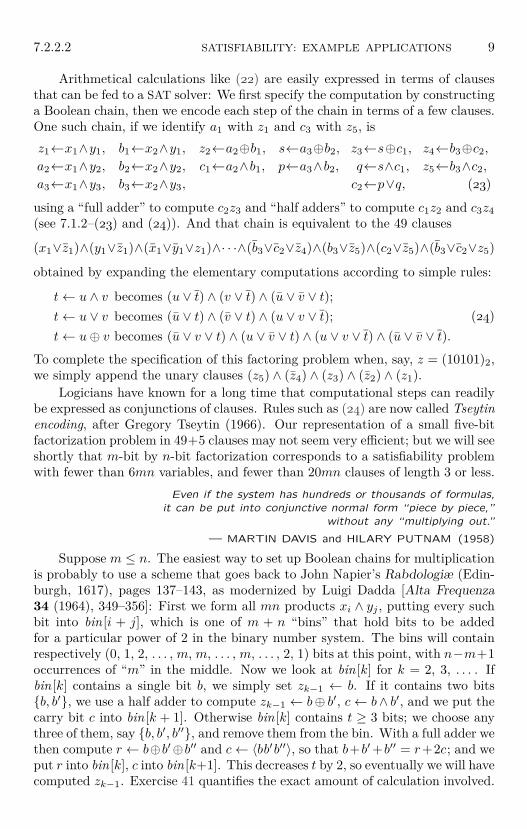
Fault testing. Lots of things can go wrong when computer chips are manufac-tured in the “real world,” so engineers have long been interested in constructingtest patterns to check the validity of a particular circuit. For example, supposethat all but one of the logical elements are functioning properly in some chip; thebad one, however, is stuck: Its output is constant, always the same regardless ofthe inputs that it is given. Such a failure is called a single-stuck-at fault.

x1x2y1y2y3

z1z2z3z4z5

z1b1a2b2a3b3

z2c1sp

z3q

c2

z4z5

Fig. 34. A circuit thatcorresponds to (23).

Figure 34 illustrates a typical digital circuit indetail: It implements the 15 Boolean operationsof (23) as a network that produces five output sig-nals z5z4z3z2z1 from the five inputs y3y2y1x2x1.In addition to having 15 AND, OR, and XOR gates,each of which transforms two inputs into one out-put, it has 15 “fanout” gates (indicated by dots atjunction points), each of which splits one inputinto two outputs. As a result it comprises 50potentially distinct logical signals, one for eachinternal “wire.” Exercise 47 shows that a circuitwith m outputs, n inputs, and g conventional 2-to-1 gates will have g + m − n fanout gates and3g+ 2m− n wires. A circuit with w wires has 2wpossible single-stuck-at faults, namely w faults inwhich the signal on a wire is stuck at 0 and wmore on which it is stuck at 1.

Table 1 shows 101 scenarios that are possiblewhen the 50 wires of Fig. 34 are activated by oneparticular sequence of inputs, assuming that at

7.2.2.2 SATISFIABILITY: EXAMPLE APPLICATIONS 11

Table 1SINGLE-STUCK-AT FAULTS IN FIGURE 34 WHEN x2x1 = 11, y3y2y1 = 110

OK x1x11x2

1x31x4

1x2x12x2

2x32x4

2y1y11 y2

1 y2y12 y2

2 y3y13 y2

3 z1 a2a12a2

2a3a13a2

3 b1 b11 b2

1 b2 b12 b2

2 b3 b13 b2

3 z2 c1 c11 c2

1 s s1 s2 p z3 q c2 c12 c2

2 z4 z5x1←input 1 00011111111111111111111111111111111111111111111111111111111111111111111111111111111111111111111111111111

x11←x1 1 01000111111111111111111111111111111111111111111111111111111111111111111111111111111111111111111111111111

x21←x1 1 01110001111111111111111111111111111111111111111111111111111111111111111111111111111111111111111111111111

x31←x1

1 1 01011100011111111111111111111111111111111111111111111111111111111111111111111111111111111111111111111111

x41←x1

1 1 01011111000111111111111111111111111111111111111111111111111111111111111111111111111111111111111111111111

x2←input 1 11111111110001111111111111111111111111111111111111111111111111111111111111111111111111111111111111111111

x12←x2 1 11111111110100011111111111111111111111111111111111111111111111111111111111111111111111111111111111111111

x22←x2 1 11111111110111000111111111111111111111111111111111111111111111111111111111111111111111111111111111111111

x32←x1

2 1 11111111110101110001111111111111111111111111111111111111111111111111111111111111111111111111111111111111

x42←x1

2 1 11111111110101111100011111111111111111111111111111111111111111111111111111111111111111111111111111111111

y1←input 0 00000000000000000000000111000000000000000000000000000000000000000000000000000000000000000000000000000000

y11←y1 0 00000000000000000000010001110000000000000000000000000000000000000000000000000000000000000000000000000000

y21←y1 0 00000000000000000000010000011100000000000000000000000000000000000000000000000000000000000000000000000000

y2←input 1 11111111111111111111111111000111111111111111111111111111111111111111111111111111111111111111111111111111

y12←y2 1 11111111111111111111111111010001111111111111111111111111111111111111111111111111111111111111111111111111

y22←y2 1 11111111111111111111111111011100011111111111111111111111111111111111111111111111111111111111111111111111

y3←input 1 11111111111111111111111111111111000111111111111111111111111111111111111111111111111111111111111111111111

y13←y3 1 11111111111111111111111111111111010001111111111111111111111111111111111111111111111111111111111111111111

y23←y3 1 11111111111111111111111111111111011100011111111111111111111111111111111111111111111111111111111111111111

z1←x21∧y1

1 0 00000000000000000000010100000000000000000111000000000000000000000000000000000000000000000000000000000000

a2←x31∧y1

2 1 01011101111111111111111111010111111111110001111111111111111111111111111111111111111111111111111111111111

a12←a2 1 01011101111111111111111111010111111111110100011111111111111111111111111111111111111111111111111111111111

a22←a2 1 01011101111111111111111111010111111111110111000111111111111111111111111111111111111111111111111111111111

a3←x41∧y1

3 1 01011111011111111111111111111111010111111111110001111111111111111111111111111111111111111111111111111111

a13←a3 1 01011111011111111111111111111111010111111111110100011111111111111111111111111111111111111111111111111111

a23←a3 1 01011111011111111111111111111111010111111111110111000111111111111111111111111111111111111111111111111111

b1←x22∧y2

1 0 00000000000000000000010001000000000000000000000000000001110000000000000000000000000000000000000000000000

b11←b1 0 00000000000000000000010001000000000000000000000000000100011100000000000000000000000000000000000000000000

b21←b1 0 00000000000000000000010001000000000000000000000000000100000111000000000000000000000000000000000000000000

b2←x32∧y2

2 1 11111111110101110111111111011101111111111111111111111111110001111111111111111111111111111111111111111111

b12←b2 1 11111111110101110111111111011101111111111111111111111111110100011111111111111111111111111111111111111111

b22←b2 1 11111111110101110111111111011101111111111111111111111111110111000111111111111111111111111111111111111111

b3←x42∧y2

3 1 11111111110101111101111111111111011101111111111111111111111111110001111111111111111111111111111111111111

b13←b3 1 11111111110101111101111111111111011101111111111111111111111111110100011111111111111111111111111111111111

b23←b3 1 11111111110101111101111111111111011101111111111111111111111111110111000111111111111111111111111111111111

z2←a12⊕b1

1 1 01011101111111111111101110010111111111110101111111111010111111111111110001111111111111111111111111111111

c1←a22∧b2

1 0 00000000000000000000010001000000000000000000000000000100010000000000000000011100000000000000000000000000

c11←c1 0 00000000000000000000010001000000000000000000000000000100010000000000000001000111000000000000000000000000

c21←c1 0 00000000000000000000010001000000000000000000000000000100010000000000000001000001110000000000000000000000

s←a13⊕b1

2 0 10100000101010001000000000100010101000000000001010000000001010000000000000000000011100000000000000000000

s1←s 0 10100000101010001000000000100010101000000000001010000000001010000000000000000001000111000000000000000000

s2←s 0 10100000101010001000000000100010101000000000001010000000001010000000000000000001000001110000000000000000

p←a23∧b2

2 1 01011111010101110111111111011101010111111111110111011111110111011111111111111111111100011111111111111111

z3←s1⊕c11 0 10100000101010001000010001100010101000000000001010000100011010000000000001010001010000000111000000000000

q←s2∧c21 0 00000000000000000000000000000000000000000000000000000000000000000000000000000000000000000001110000000000

c2←p∨q 1 01011111010101110111111111011101010111111111110111011111110111011111111111111111111101111100011111111111

c12←c2 1 01011111010101110111111111011101010111111111110111011111110111011111111111111111111101111101000111111111

c22←c2 1 01011111010101110111111111011101010111111111110111011111110111011111111111111111111101111101110001111111

z4←b13⊕c1

2 0 10100000100000001010000000100010001010000000001000100000001000101010000000000000000010000010100000011100

z5←b23∧c2

2 1 01011111010101110101111111011101010101111111110111011111110111010111011111111111111101111101110111000111

most one stuck-at fault is present. The column headed OK shows the correctbehavior of the Boolean chain (which nicely multiplies x = 3 by y = 6 andobtains z = 18). We can call these the “default” values, because, well, they haveno faults. The other 100 columns show what happens if all but one of the 50wires have error-free signals; the two columns under b1

2, for example, illustratethe results when the rightmost wire that fans out from gate b2 is stuck at 0or 1. Each row is obtained bitwise from previous rows or inputs, except that theboldface digits are forced. When a boldface value agrees with the default, itsentire column is correct; otherwise errors might propagate. All values above thebold diagonal match the defaults.

If we want to test a chip that has n inputs and m outputs, we’re allowedto apply test patterns to the inputs and see what outputs are produced. Close

12 COMBINATORIAL SEARCHING (F6) 7.2.2.2

inspection shows, for instance, that the pattern considered in Table 1 doesn’tdetect an error when q is stuck at 1, even though q should be 0, because all fiveoutput bits z5z4z3z2z1 are correct in spite of that error. In fact, the value ofc2 ← p ∨ q is unaffected by a bad q, because p = 1 in this example. Similarly,the fault “x2

1 stuck at 0” doesn’t propagate into z1 ← x21 ∧ y1

1 because y11 = 0.

Altogether 44 faults, not 50, are discovered by this particular test pattern.All of the relevant repeatable faults, whether they’re single-stuck-at or wildly

complicated, could obviously be discovered by testing all 2n possible patterns.But that’s out of the question unless n is quite small. Fortunately, testing isn’thopeless, because satisfactory results are usually obtained in practice if we dohave enough test patterns to detect all of the detectable single-stuck-at faults.Exercise 49 shows that just five patterns suffice to certify Fig. 34 by this criterion.

The detailed analysis in exercise 49 also shows, surprisingly, that one of thefaults, namely “s2 stuck at 1,” cannot be detected! Indeed, an erroneous s2 canpropagate to an erroneous q only if c2

1 = 1, and that forces x1 = x2 = y1 = y2 = 1;only two possibilities remain, and neither y3 = 0 nor y3 = 1 reveals the fault.Consequently we can simplify the circuit by removing gate q ; the chain (23)becomes shorter, with “q ← s ∧ c1, c2 ← p∨ q” replaced by “c2 ← p∨ c1.”

Of course Fig. 34 is just a tiny little circuit, intended only to introduce theconcept of stuck-at faults. Test patterns are needed for the much larger circuitsthat arise in real computers; and we will see that SAT solvers can help us to findthem. Consider, for example, the generic multiplier circuit prod (m,n), which ispart of the Stanford GraphBase. It multiplies an m-bit number x by an n-bitnumber y, producing an (m + n)-bit product z. Furthermore, it’s a so-called“parallel multiplier,” with delay time O(log(m+n)); thus it’s much more suitedto hardware design than methods like the factor fifo schemes that we consideredabove, because those circuits need Ω(m+ n) time for carries to propagate.

Let’s try to find test patterns that will smoke out all of the single-stuck-atfaults in prod (32, 32), which is a circuit of depth 33 that has 64 inputs, 64 out-puts, 3660 AND gates, 1203 OR gates, 2145 XOR gates, and (therefore) 7008 fan-out gates and 21,088 wires. How can we guard it against 42,176 different faults?

Before we construct clauses to facilitate that task, we should realize thatmost of the single-stuck-at faults are easily detected by choosing patterns atrandom, since faults usually cause big trouble and are hard to miss. Indeed,choosing x = #3243F6A8 and y = #885A308D more or less at random alreadyeliminates 14,733 cases; and (x, y) = (#2B7E1516, #28AED2A6) eliminates 6,918more. We might as well keep doing this, because bitwise operations such as thosein Table 1 are fast. Experience with the smaller multiplier in Fig. 34 suggeststhat we get more effective tests if we bias the inputs, choosing each bit to be 1with probability .9 instead of .5 (see exercise 49). A million such random inputswill then generate, say, 243 patterns that detect all but 140 of the faults.

Our remaining job, then, is essentially to find 140 needles in a haystack ofsize 264, after having picked 42,176 − 140 = 42,036 pieces of low-hanging fruit.And that’s where a SAT solver is useful. Consider, for example, the analogousbut simpler problem of finding a test pattern for “q stuck at 0” in Fig. 34.

7.2.2.2 SATISFIABILITY: EXAMPLE APPLICATIONS 13

We can use the 49 clauses F derived from (23) to represent the well-behavedcircuit; and we can imagine corresponding clauses F ′ that represent the faultycomputation, using “primed” variables z′1, a′2, . . . , z′5. Thus F ′ begins with(x1∨ z′1)∧(y1∨ z′1) and ends with (b′3∨ c′2∨z′5); it’s like F except that the clausesrepresenting q′ ← s′∧ c′1 in (23) are changed to simply q′ (meaning that q′ isstuck at 0). Then the clauses of F and F ′, together with a few more clauses tostate that z1 = z′1 or · · · or z5 = z′5, will be satisfiable only by variables for which(y3y2y1)2 × (x2x1)2 is a suitable test pattern for the given fault.

This construction of F ′ can obviously be simplified, because z′1 is identicalto z1; any signal that differs from the correct value must be located “downstream”from the one-and-only fault. Let’s say that a wire is tarnished if it is the faultywire or if at least one of its input wires is tarnished. We introduce new variablesg′ only for wires g that are tarnished. Thus, in our example, the only clauses F ′

that are needed to extend F to a faulty companion circuit are q′ and the clausesthat correspond to c′2 ← p ∨ q′, z′4 ← b3 ⊕ c′2, z′5 ← b3 ∧ c′2.

Moreover, any fault that is revealed by a test pattern must have an activepath of wires, leading from the fault to an output; all wires on this path mustcarry a faulty signal. Therefore Tracy Larrabee [IEEE Trans. CAD-11 (1992),4–15] decided to introduce additional “sharped” variables g♯ for each tarnishedwire, meaning that g lies on the active path. The two clauses

(g♯ ∨ g ∨ g′) ∧ (g♯ ∨ g ∨ g′) (25)

ensure that g = g′ whenever g is part of that path. Furthermore we have (v♯∨g♯)whenever g is an AND, OR, or XOR gate with tarnished input v. Fanout gatesare slightly tricky in this regard: When wires g1 and g2 fan out from a tarnishedwire g, we need variables g1♯ and g2♯ as well as g♯; and we introduce the clause

(g♯ ∨ g1♯ ∨ g2♯) (26)

to specify that the active path takes at least one of the two branches.According to these rules, our example acquires the new variables q♯, c♯2, c1♯

2 ,c2♯

2 , z♯4, z♯5, and the new clauses

(q♯∨q∨q′)∧ (q♯∨ q∨ q′)∧ (q♯∨c♯2)∧ (c♯2∨c2∨c′2)∧ (c♯2∨ c2∨ c′2)∧ (c♯2∨c1♯2 ∨c

2♯2 )∧

(c1♯2 ∨z

♯4)∧ (z♯4∨z4∨z′4)∧ (z♯4∨ z4∨ z′4)∧ (c2♯

2 ∨z♯5)∧ (z♯5∨z5∨z′5)∧ (z♯5∨ z5∨ z′5).

The active path begins at q, so we assert the unit clause (q♯); it ends at atarnished output, so we also assert (z♯4 ∨ z

♯5). The resulting set of clauses will

find a test pattern for this fault if and only if the fault is detectable. Larrabeefound that such active-path variables provide important clues to a SAT solverand significantly speed up the solution process.

Returning to the large circuit prod (32, 32), one of the 140 hard-to-test faultsis “W 26

21 stuck at 1,” where W 2621 denotes the 26th extra wire that fans out from

the OR gate called W21 in §75 of the Stanford GraphBase program GB GATES;W 26

21 is an input to gate b4040 ← d19

40 ∧W 2621 in §80 of that program. Test patterns

for that fault can be characterized by a set of 23,194 clauses in 7,082 variables

14 COMBINATORIAL SEARCHING (F6) 7.2.2.2

(of which only 4 variables are “primed” and 4 are “sharped”). Fortunatelythe solution (x, y) = (#7F13FEDD, #5FE57FFE) was found rather quickly in theauthor’s experiments; and this pattern also killed off 13 of the other cases, sothe score was now “14 down and 126 to go”!

The next fault sought was “A36,25 stuck at 1,” where A36,2

5 is the secondextra wire to fan out from the AND gate A36

5 in §72 of GB GATES (an inputto R36

11 ← A36,25 ∧ R35,2

1 ). This fault corresponds to 26,131 clauses on 8,342variables; but the SAT solver took a quick look at those clauses and decidedalmost instantly that they are unsatisfiable. Therefore the fault is undetectable,and the circuit prod (32, 32) can be simplified by setting R36

11 ← R35,21 . A closer

look showed, in fact, that clauses corresponding to the Boolean equations

x = y ∧ z, y = v ∧ w, z = t ∧ u, u = v ⊕ w

were present (where t = R4413, u = A45

58, v = R444 , w = A45

14, x = R4623, y = R45

13,z = R45

19); these clauses force x = 0. Therefore it was not surprising to findthat the list of unresolved faults also included R46

23, R46,123 and R46,2

23 stuck at 0.Altogether 26 of the 140 faults undetected by random inputs turned out to beabsolutely undetectable; and only one of these, namely “Q46

26 stuck at 0,” requireda nontrivial proof of undetectability.

Some of the 126−26 = 100 faults remaining on the to-do list turned out to besignificant challenges for the SAT solver. While waiting, the author therefore hadtime to take a look at a few of the previously found solutions, and noticed thatthose patterns themselves were forming a pattern! Sure enough, the extreme por-tions of this large and complicated circuit actually have a fairly simple structure,stuck-at-fault-wise. Hence number theory came to the rescue: The factorization#87FBC059 × #F0F87817 = 263 − 1 solved many of the toughest challenges,some of which occur with probability less than 2−34 when 32-bit numbers aremultiplied; and the “Aurifeuillian” factorization (231 − 216 + 1)(231 + 216 + 1) =262 + 1, which the author had known for more than forty years (see Eq. 4.5.4–(15)), polished off most of the others.

The bottom line (see exercise 51) is that all 42,150 of the detectable single-stuck-at faults of the parallel multiplication circuit prod (32, 32) can actually bedetected with at most 196 well-chosen test patterns.

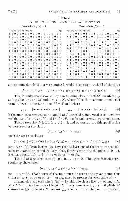
Learning a Boolean function. Sometimes we’re given a “black box” thatevaluates a Boolean function f(x1, . . . , xN ). We have no way to open the box,but we suspect that the function is actually quite simple. By plugging in variousvalues for x = x1 . . . xN , we can observe the box’s behavior and possibly learn thehidden rule that lies inside. For example, a secret function of N = 20 Booleanvariables might take on the values shown in Table 2, which lists 16 cases wheref(x) = 1 and 16 cases where f(x) = 0.

Suppose we assume that the function has a DNF (disjunctive normal form)with only a few terms. We’ll see in a moment that it’s easy to express such anassumption as a satisfiability problem. And when the author constructed clausescorresponding to Table 2 and presented them to a SAT solver, he did in fact learn

7.2.2.2 SATISFIABILITY: EXAMPLE APPLICATIONS 15

Table 2VALUES TAKEN ON BY AN UNKNOWN FUNCTION

Cases where f(x) = 1x1x2x3x4x5x6x7x8x9 . . . x20

1 1 0 0 1 0 0 1 0 0 0 0 1 1 1 1 1 1 0 11 0 1 0 1 0 1 0 0 0 1 0 0 0 1 0 0 0 0 10 1 1 0 1 0 0 0 1 1 0 0 0 0 1 0 0 0 1 10 1 0 0 1 1 0 0 0 1 0 0 1 1 0 0 0 1 1 00 1 1 0 0 0 1 0 1 0 0 0 1 0 1 1 1 0 0 00 0 0 0 1 1 0 1 1 1 0 0 0 0 0 1 1 1 0 01 1 0 1 0 0 0 1 0 0 1 0 1 0 0 1 0 0 0 00 0 1 0 0 1 0 0 1 1 1 0 0 0 0 0 1 0 0 01 0 0 0 1 0 1 0 0 1 1 0 0 1 1 1 1 1 0 01 1 0 0 0 1 1 1 0 1 0 0 0 0 0 0 0 0 1 00 0 0 0 1 0 1 1 1 0 1 1 1 1 1 0 1 0 1 00 1 1 0 0 0 1 1 1 0 1 1 0 0 0 1 0 0 1 11 0 0 1 1 0 1 1 0 0 1 0 0 0 1 0 0 1 0 10 0 0 1 0 1 0 0 1 0 1 0 0 0 0 0 1 0 0 00 1 1 1 1 0 0 1 1 0 0 0 1 1 1 0 0 0 1 10 1 0 0 0 0 0 0 0 1 0 0 1 1 0 1 1 1 0 1

Cases where f(x) = 0x1x2x3x4x5x6x7x8x9 . . . x20

1 0 1 0 1 1 0 1 1 1 1 1 1 0 0 0 0 1 0 10 1 0 0 0 1 0 1 1 0 0 0 1 0 1 0 0 0 1 01 0 1 1 1 0 1 1 0 1 0 0 1 0 1 0 1 0 0 11 0 1 0 1 0 1 0 1 1 1 1 1 1 0 1 1 1 0 00 1 0 1 0 1 1 0 0 0 1 0 0 0 0 0 0 0 1 00 1 1 1 0 0 1 1 1 1 0 1 0 0 1 1 1 1 0 01 1 1 1 0 0 0 1 1 1 0 1 1 0 0 0 1 0 1 11 0 0 1 1 1 0 0 0 1 0 1 1 0 0 0 0 0 1 11 1 0 0 1 1 1 0 0 0 1 0 1 1 0 1 0 0 1 10 1 1 0 1 0 0 1 0 1 0 1 1 0 1 0 1 0 0 11 1 1 0 0 0 0 1 0 0 1 1 0 1 1 0 0 1 0 00 0 0 1 0 0 0 1 0 1 0 0 0 1 1 0 0 1 0 00 0 1 1 0 0 1 1 1 1 1 1 1 0 1 1 1 1 0 01 1 0 0 1 0 0 1 0 0 1 1 1 0 0 1 1 1 0 11 1 0 0 1 1 1 0 0 0 1 0 0 1 0 0 1 0 0 11 0 1 1 0 0 1 1 1 1 1 0 1 1 1 1 1 0 0 1

almost immediately that a very simple formula is consistent with all of the data:

f(x1, . . . , x20) = x2x3x10 ∨ x6x10x12 ∨ x8x13x15 ∨ x8x10x12. (27)

This formula was discovered by constructing clauses in 2MN variables pi,jand qi,j for 1 ≤ i ≤ M and 1 ≤ j ≤ N , where M is the maximum number ofterms allowed in the DNF (here M = 4) and where

pi,j = [term i contains xj ], qi,j = [term i contains xj ]. (28)

If the function is constrained to equal 1 at P specified points, we also use auxiliaryvariables zi,k for 1 ≤ i ≤M and 1 ≤ k ≤ P , one for each term at every such point.

Table 2 says that f(1, 1, 0, 0, . . . , 1) = 1, and we can capture this specificationby constructing the clause

(z1,1 ∨ z2,1 ∨ · · · ∨ zM,1) (29)together with the clauses

(zi,1∨ qi,1) ∧ (zi,1∨ qi,2) ∧ (zi,1∨ pi,3) ∧ (zi,1∨ pi,4) ∧ · · · ∧ (zi,1∨ qi,20) (30)

for 1 ≤ i ≤M . Translation: (29) says that at least one of the terms in the DNFmust evaluate to true; and (30) says that, if term i is true at the point 1100 . . . 1,it cannot contain x1 or x2 or x3 or x4 or · · · or x20.

Table 2 also tells us that f(1, 0, 1, 0, . . . , 1) = 0. This specification corre-sponds to the clauses

(qi,1 ∨ pi,2 ∨ qi,3 ∨ pi,4 ∨ · · · ∨ qi,20) (31)

for 1 ≤ i ≤ M . (Each term of the DNF must be zero at the given point; thuseither x1 or x2 or x3 or x4 or · · · or x20 must be present for each value of i.)

In general, every case where f(x) = 1 yields one clause like (29) of length M,plus MN clauses like (30) of length 2. Every case where f(x) = 0 yields Mclauses like (31) of length N . We use qi,j when xj = 1 at the point in question,

16 COMBINATORIAL SEARCHING (F6) 7.2.2.2

and pi,j when xj = 0, for both (30) and (31). This construction is due toA. P. Kamath, N. K. Karmarkar, K. G. Ramakrishnan, and M. G. C. Resende[Mathematical Programming 57 (1992), 215–238], who presented many exam-ples. From Table 2, with M = 4, N = 20, and P = 16, it generates 1360 clausesof total length 3904 in 224 variables; a SAT solver then finds a solution withp1,1 = q1,1 = p1,2 = 0, q1,2 = 1, . . . , leading to (27).

The simplicity of (27) makes it plausible that the SAT solver has indeedpsyched out the true nature of the hidden function f(x). The chance of agreeingwith the correct value 32 times out of 32 is only 1 in 232, so we seem to haveoverwhelming evidence in favor of that equation.

But no: Such reasoning is fallacious. The numbers in Table 2 actually arosein a completely different way, and Eq. (27) has essentially no credibility as apredictor of f(x) for any other values of x! (See exercise 53.) The fallacy comesfrom the fact that short-DNF Boolean functions of 20 variables are not at allrare; there are many more than 232 of them.

On the other hand, when we do know that the hidden function f(x) hasa DNF with at most M terms (although we know nothing else about it), theclauses (29)–(31) give us a nice way to discover those terms, provided that wealso have a sufficiently large and unbiased “training set” of observed values.

For example, let’s assume that (27) actually is the function in the box. Ifwe examine f(x) at 32 random points x, we don’t have enough data to makeany deductions. But 100 random training points will almost always home in onthe correct solution (27). This calculation typically involves 3942 clauses in 344variables; yet it goes quickly, needing only about 100 million accesses to memory.

One of the author’s experiments with a 100-element training set yielded

f(x1, . . . , x20) = x2x3x10 ∨ x3x6x10x12 ∨ x8x13x15 ∨ x8x10x12, (32)

which is close to the truth but not quite exact. (Exercise 59 proves that f(x)is equal to f(x) more than 97% of the time.) Further study of this exampleshowed that another nine training points were enough to deduce f(x) uniquely,thus obtaining 100% confidence (see exercise 61).

Bounded model checking. Some of the most important applications of SATsolvers in practice are related to the verification of hardware or software, becausedesigners generally want some kind of assurance that particular implementationscorrectly meet their specifications.

A typical design can usually be modeled as a transition relation betweenBoolean vectors X = x1 . . . xn that represent the possible states of a system. Wewrite X → X ′ if state X at time t can be followed by state X ′ at time t + 1.The task in general is to study sequences of state transitions

X0 → X1 → X2 → · · · → Xr, (33)

and to decide whether or not there are sequences that have special properties.For example, we hope that there’s no such sequence for which X0 is an “initialstate” and Xr is an “error state”; otherwise there’d be a bug in the design.

7.2.2.2 SATISFIABILITY: EXAMPLE APPLICATIONS 17

→ → →

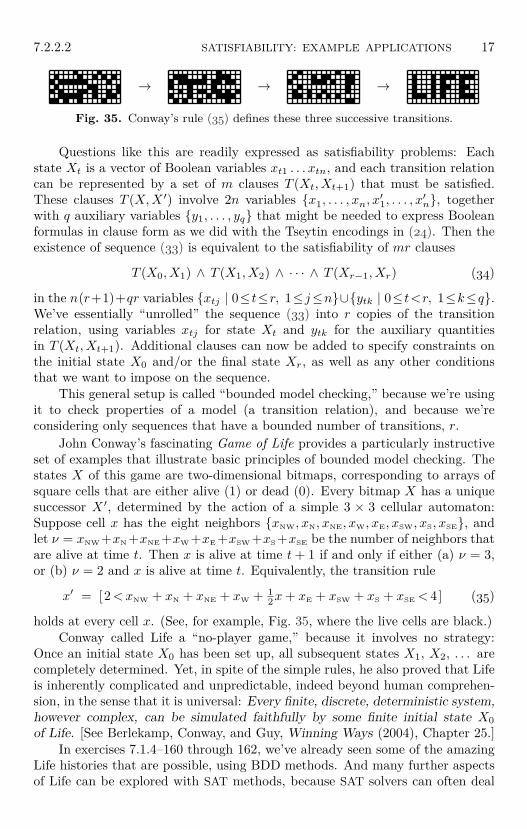
Fig. 35. Conway’s rule (35) defines these three successive transitions.

Questions like this are readily expressed as satisfiability problems: Eachstate Xt is a vector of Boolean variables xt1 . . . xtn, and each transition relationcan be represented by a set of m clauses T (Xt, Xt+1) that must be satisfied.These clauses T (X,X ′) involve 2n variables x1, . . . , xn, x

′1, . . . , x

′n, together

with q auxiliary variables y1, . . . , yq that might be needed to express Booleanformulas in clause form as we did with the Tseytin encodings in (24). Then theexistence of sequence (33) is equivalent to the satisfiability of mr clauses

T (X0, X1) ∧ T (X1, X2) ∧ · · · ∧ T (Xr−1, Xr) (34)

in the n(r+1)+qr variables xtj | 0≤ t≤r, 1≤j≤n∪ytk | 0≤ t<r, 1≤k≤q.We’ve essentially “unrolled” the sequence (33) into r copies of the transitionrelation, using variables xtj for state Xt and ytk for the auxiliary quantitiesin T (Xt, Xt+1). Additional clauses can now be added to specify constraints onthe initial state X0 and/or the final state Xr, as well as any other conditionsthat we want to impose on the sequence.

This general setup is called “bounded model checking,” because we’re usingit to check properties of a model (a transition relation), and because we’reconsidering only sequences that have a bounded number of transitions, r.

John Conway’s fascinating Game of Life provides a particularly instructiveset of examples that illustrate basic principles of bounded model checking. Thestates X of this game are two-dimensional bitmaps, corresponding to arrays ofsquare cells that are either alive (1) or dead (0). Every bitmap X has a uniquesuccessor X ′, determined by the action of a simple 3 × 3 cellular automaton:Suppose cell x has the eight neighbors xNW, xN, xNE, xW, xE, xSW, xS, xSE, andlet ν = xNW +xN +xNE +xW +xE +xSW +xS +xSE be the number of neighbors thatare alive at time t. Then x is alive at time t+ 1 if and only if either (a) ν = 3,or (b) ν = 2 and x is alive at time t. Equivalently, the transition rule

x′ = [2<xNW + xN + xNE + xW + 12x+ xE + xSW + xS + xSE < 4] (35)

holds at every cell x. (See, for example, Fig. 35, where the live cells are black.)Conway called Life a “no-player game,” because it involves no strategy:

Once an initial state X0 has been set up, all subsequent states X1, X2, . . . arecompletely determined. Yet, in spite of the simple rules, he also proved that Lifeis inherently complicated and unpredictable, indeed beyond human comprehen-sion, in the sense that it is universal: Every finite, discrete, deterministic system,however complex, can be simulated faithfully by some finite initial state X0of Life. [See Berlekamp, Conway, and Guy, Winning Ways (2004), Chapter 25.]

In exercises 7.1.4–160 through 162, we’ve already seen some of the amazingLife histories that are possible, using BDD methods. And many further aspectsof Life can be explored with SAT methods, because SAT solvers can often deal

18 COMBINATORIAL SEARCHING (F6) 7.2.2.2

with many more variables. For example, Fig. 35 was discovered by using 7×15 =105 variables for each state X0, X1, X2, X3. The values of X3 were obviouslypredetermined; but the other 105× 3 = 315 variables had to be computed, andBDDs can’t handle that many. Moreover, additional variables were introducedto ensure that the initial state X0 would have as few live cells as possible.

Here’s the story behind Fig. 35, in more detail: Since Life is two-dimensional,we use variables xij instead of xj to indicate the states of individual cells, and xtijinstead of xtj to indicate the states of cells at time t. We generally assume thatxtij = 0 for all cells outside of a given finite region, although the transition rule(35) can allow cells that are arbitrarily far away to become alive as Life goes on.In Fig. 35 the region was specified to be a 7× 15 rectangle at each unit of time.Furthermore, configurations with three consecutive live cells on a boundary edgewere forbidden, so that cells “outside the box” wouldn’t be activated.

The transitions T (Xt, Xt+1) can be encoded without introducing additionalvariables, but only if we introduce 190 rather long clauses for each cell not on theboundary. There’s a better way, based on the binary tree approach underlying(20) and (21) above, which requires only about 63 clauses of size ≤ 3, togetherwith about 14 auxiliary variables per cell. This approach (see exercise 65) takesadvantage of the fact that many intermediate calculations can be shared. Forexample, cells x and xW have four neighbors xNW, xN, xSW, xS in common; sowe need to compute xNW + xN + xSW + xS only once, not twice.

The clauses that correspond to a four-step sequence X0 → X1 → X2 →X3 → X4 leading to X4 = turn out to be unsatisfiable without goingoutside of the 7 × 15 frame. (Only 10 gigamems of calculation were needed toestablish this fact, using Algorithm C below, even though roughly 34000 clausesin 9000 variables needed to be examined!) So the next step in the preparationof Fig. 35 was to try X3 = ; and this trial succeeded. Additional clauses,which permitted X0 to have at most 39 live cells, led to the solution shown, at acost of about 17 gigamems; and that solution is optimum, because a further run(costing 12 gigamems) proved that there’s no solution with at most 38.

Let’s look for a moment at some of the patterns that can occur on achessboard, an 8×8 grid. Human beings will never be able to contemplate morethan a tiny fraction of the 264 states that are possible; so we can be fairly surethat “Lifenthusiasts” haven’t already explored every tantalizing configurationthat exists, even on such a small playing field.

One nice way to look for a sequence of interesting Life transitions is to assertthat no cell stays alive more than four steps in a row. Let us therefore say thata mobile Life path is a sequence of transitions X0 → X1 → · · · → Xr with theadditional property that we have

(xtij ∨ x(t+1)ij ∨ x(t+2)ij ∨ x(t+3)ij ∨ x(t+4)ij), for 0 ≤ t ≤ r − 4. (36)

To avoid trivial solutions we also insist that Xr is not entirely dead. For example,if we impose rule (36) on a chessboard, with xtij permitted to be alive only if1 ≤ i, j ≤ 8, and with the further condition that at most five cells are alive in each

7.2.2.2 SATISFIABILITY: EXAMPLE APPLICATIONS 19

generation, a SAT solver can quickly discover interesting mobile paths such as

→ → → → → → → → → · · · , (37)

which last quite awhile before leaving the board. And indeed, the five-celledobject that moves so gracefully in this path is R. K. Guy’s famous glider (1970),which is surely the most interesting small creature in Life’s universe. The glidermoves diagonally, recreating a shifted copy of itself after every four steps.

Interesting mobile paths appear also if we restrict the population at eachtime to 6, 7, 8, 9, 10 instead of 1, 2, 3, 4, 5. For example, here are some of thefirst such paths that the author’s solver came up with, having length r = 8:

→ → → → → → → → ;

→ → → → → → → → ;

→ → → → → → → → ;

→ → → → → → → → ;

→ → → → → → → → .

These paths illustrate the fact that symmetry can be gained, but never lost, asLife evolves deterministically. Marvelous designs are spawned in the process.In each of these sequences the next bitmap, X9, would break our ground rules:The population immediately after X8 grows to 12 in the first and last examples,but shrinks to 5 in the second-from-last; and the path becomes immobile in theother two. Indeed, we have X5 = X7 in the second example, hence X6 = X8and X7 = X9, etc. Such a repeating pattern is called an oscillator of period 2.The third example ends with an oscillator of period 1, known as a “still life.”

What are the ultimate destinations of these paths? The first one becomesstill, with X69 = X70; and the fourth becomes very still, with X12 = 0! Thefifth is the most fascinating of the group, because it continues to produce evermore elaborate valentine shapes, then proceeds to dance and sparkle, until finallybeginning to twinkle with period 2 starting at time 177. Thus its members X2through X7 qualify as “Methuselahs,” defined by Martin Gardner as “Life pat-terns of population less than 10 that do not become stable within 50 generations.”(A predictable pattern, like the glider or an oscillator, is called stable.)

SAT solvers are basically useless for the study of Methuselahs, because thestate space becomes too large. But they are quite helpful when we want toilluminate many other aspects of Life, and exercises 66–85 discuss some notableinstances. We will consider one more instructive example before moving on,

20 COMBINATORIAL SEARCHING (F6) 7.2.2.2

namely an application to “eaters.” Consider a Life path of the form

X0 = →? ? ? ? ? ? ? ?? ? ? ? ? ? ? ?? ? ? ? ? ? ? ?? ? ? ? ? ? ? ?? ? ? ? ? ? ? ?? ? ? ? ? ? ? ?? ? ? ? ? ? ? ?? ? ? ? ? ? ? ?

→? ? ? ? ? ? ? ?? ? ? ? ? ? ? ?? ? ? ? ? ? ? ?? ? ? ? ? ? ? ?? ? ? ? ? ? ? ?? ? ? ? ? ? ? ?? ? ? ? ? ? ? ?? ? ? ? ? ? ? ?

→? ? ? ? ? ? ? ?? ? ? ? ? ? ? ?? ? ? ? ? ? ? ?? ? ? ? ? ? ? ?? ? ? ? ? ? ? ?? ? ? ? ? ? ? ?? ? ? ? ? ? ? ?? ? ? ? ? ? ? ?

→ → = X5, (38)

where the gray cells form a still life and the cells of X1, X2, X3 are unknown.Thus X4 = X5 and X0 = X5 + glider. Furthermore we require that the stilllife X5 does not interact with the glider’s parent, ; see exercise 77. The ideais that a glider will be gobbled up if it happens to glide into this particular stilllife, and the still life will rapidly reconstitute itself as if nothing had happened.

Algorithm C almost instantaneously (well, after about 100 megamems) finds

→ → → → → , (39)

the four-step eater first observed in action by R. W. Gosper in 1971.

Applications to mutual exclusion. Let’s look now at how bounded modelchecking can help us to prove that algorithms are correct. (Or incorrect.) Someof the most challenging issues of verification arise when we consider parallelprocesses that need to synchronize their concurrent behavior. To simplify ourdiscussion it will be convenient to tell a little story about Alice and Bob.

Alice and Bob are casual friends who share an apartment. One of their jointrooms is special: When they’re in that critical room, which has two doors, theydon’t want the other person to be present. Furthermore, being busy people, theydon’t want to interrupt each other needlessly. So they agree to control access tothe room by using an indicator light, which can be switched on or off.

The first protocol they tried can be characterized by symmetrical algorithms:

A0. Maybe go to A1.A1. If l go to A1, else to A2.A2. Set l← 1, go to A3.A3. Critical, go to A4.A4. Set l← 0, go to A0.

B0. Maybe go to B1.B1. If l go to B1, else to B2.B2. Set l← 1, go to B3.B3. Critical, go to B4.B4. Set l← 0, go to B0.

(40)

At any instant of time, Alice is in one of five states, A0,A1,A2,A3,A4, andthe rules of her program show how that state might change. In state A0 she isn’tinterested in the critical room; but she goes to A1 when she does wish to useit. She reaches that objective in state A3. Similar remarks apply to Bob. Whenthe indicator light is on (l = 1), they wait until the other person has exited theroom and switched the light back off (l = 0).

Alice and Bob don’t necessarily operate at the same speed. But they’reallowed to dawdle only when in the “maybe” state A0 or B0. More precisely, wemodel the situation by converting every relevant scenario into a discrete sequenceof state transitions. At every time t = 0, 1, 2, . . . , either Alice or Bob (but notboth) will perform the command associated with their current state, thereby per-haps changing to a different state at time t+ 1. This choice is nondeterministic.

Only four kinds of primitive commands are permitted in the procedures weshall study, all of which are illustrated in (40): (1) “Maybe go to s”; (2) “Critical,

7.2.2.2 SATISFIABILITY: EXAMPLE APPLICATIONS 21

go to s”; (3) “Set v ← b, go to s”; and (4) “If v go to s1, else to s0”. Here sdenotes a state name, v denotes a shared Boolean variable, and b is 0 or 1.

Unfortunately, Alice and Bob soon learned that protocol (40) is unreliable:One day she went from A1 to A2 and he went from B1 to B2, before either ofthem had switched the indicator on. Embarrassment (A3 and B3) followed.

They could have discovered this problem in advance, if they’d converted thestate transitions of (40) into clauses for bounded model checking, as in (33), thenapplied a SAT solver. In this case the vector Xt that corresponds to time t con-sists of Boolean variables that encode each of their current states, as well as thecurrent value of l. We can, for example, have eleven variables A0t, A1t, A2t, A3t,A4t, B0t, B1t, B2t, B3t, B4t, lt, together with ten binary exclusion clauses (A0t∨A1t), (A0t ∨ A2t), . . . , (A3t ∨ A4t) to ensure that Alice is in at most one state,and with ten similar clauses for Bob. There’s also a variable @t, which is true orfalse depending on whether Alice or Bob executes their program step at time t.(We say that Alice was “bumped” if @t = 1, and Bob was bumped if @t = 0.)

If we start with the initial state X0 defined by unit clauses

A00 ∧ A10 ∧ A20 ∧ A30 ∧ A40 ∧ B00 ∧ B10 ∧ B20 ∧ B30 ∧ B40 ∧ l0, (41)

the following clauses for 0 ≤ t < r (discussed in exercise 87) will emulate thefirst r steps of every legitimate scenario defined by (40):

(@t ∨ A0t ∨ A0t+1)(@t ∨ A1t ∨ A1t+1)(@t ∨ A2t ∨ A2t+1)(@t ∨ A3t ∨ A3t+1)(@t ∨ A4t ∨ A4t+1)(@t ∨ B0t ∨ B0t+1)(@t ∨ B1t ∨ B1t+1)(@t ∨ B2t ∨ B2t+1)(@t ∨ B3t ∨ B3t+1)(@t ∨ B4t ∨ B4t+1)

(@t ∨ A0t ∨ A0t+1 ∨ A1t+1)(@t ∨ A1t ∨ lt ∨ A1t+1)(@t ∨ A1t ∨ lt ∨ A2t+1)(@t ∨ A2t ∨ A3t+1)(@t ∨ A2t ∨ lt+1)(@t ∨ A3t ∨ A4t+1)(@t ∨ A4t ∨ A0t+1)(@t ∨ A4t ∨ lt+1)(@t ∨ lt ∨ A2t ∨ A4t ∨ lt+1)(@t ∨ lt ∨ A2t ∨ A4t ∨ lt+1)

(@t ∨ B0t ∨ B0t+1 ∨ B1t+1)(@t ∨ B1t ∨ lt ∨ B1t+1)(@t ∨ B1t ∨ lt ∨ B2t+1)(@t ∨ B2t ∨ B3t+1)(@t ∨ B2t ∨ lt+1)(@t ∨ B3t ∨ B4t+1)(@t ∨ B4t ∨ B0t+1)(@t ∨ B4t ∨ lt+1)(@t ∨ lt ∨ B2t ∨ B4t ∨ lt+1)(@t ∨ lt ∨ B2t ∨ B4t ∨ lt+1)

(42)

If we now add the unit clauses (A3r) and (B3r), the resulting set of 13 + 50rclauses in 11+12r variables is readily satisfiable when r = 6, thereby proving thatthe critical room might indeed be jointly occupied. (Incidentally, standard termi-nology for mutual exclusion protocols would say that “two threads concurrentlyexecute a critical section”; but we shall continue with our roommate metaphor.)

Back at the drawing board, one idea is to modify (40) by letting Alice usethe room only when l = 1, but letting Bob in when l = 0:

A0. Maybe go to A1.A1. If l go to A2, else to A1.A2. Critical, go to A3.A3. Set l← 0, go to A0.

B0. Maybe go to B1.B1. If l go to B1, else to B2.B2. Critical, go to B3.B3. Set l← 1, go to B0.

(43)

Computer tests with r = 100 show that the corresponding clauses are unsatisfi-able; thus mutual exclusion is apparently guaranteed by (43).

22 COMBINATORIAL SEARCHING (F6) 7.2.2.2

But (43) is a nonstarter, because it imposes an intolerable cost: Alice can’tuse the room k times until Bob has already done so! Scrap that.

How about installing another light, so that each person controls one of them?A0. Maybe go to A1.A1. If b go to A1, else to A2.A2. Set a← 1, go to A3.A3. Critical, go to A4.A4. Set a← 0, go to A0.

B0. Maybe go to B1.B1. If a go to B1, else to B2.B2. Set b← 1, go to B3.B3. Critical, go to B4.B4. Set b← 0, go to B0.

(44)

No; this suffers from the same defect as (40). But maybe we can cleverly switchthe order of steps 1 and 2:

A0. Maybe go to A1.A1. Set a← 1, go to A2.A2. If b go to A2, else to A3.A3. Critical, go to A4.A4. Set a← 0, go to A0.

B0. Maybe go to B1.B1. Set b← 1, go to B2.B2. If a go to B2, else to B3.B3. Critical, go to B4.B4. Set b← 0, go to B0.

(45)

Yes! Exercise 95 proves easily that this protocol does achieve mutual exclusion.Alas, however, a new problem now arises, namely the problem known as

“deadlock” or “livelock.” Alice and Bob can get into states A2 and B2, afterwhich they’re stuck — each waiting for the other to go critical.

In such cases they could agree to “reboot” somehow. But that would bea cop-out; they really seek a better solution. And they aren’t alone: Manypeople have struggled with this surprisingly delicate problem over the years, andseveral solutions (both good and bad) appear in the exercises below. EdsgerDijkstra, in some pioneering lecture notes entitled Cooperating Sequential Pro-cesses [Technological University Eindhoven (September 1965), §2.1], thought ofan instructive way to improve on (45):

A0. Maybe go to A1.A1. Set a← 1, go to A2.A2. If b go to A3, else to A4.A3. Set a← 0, go to A1.A4. Critical, go to A5.A5. Set a← 0, go to A0.

B0. Maybe go to B1.B1. Set b← 1, go to B2.B2. If a go to B3, else to B4.B3. Set b← 0, go to B1.B4. Critical, go to B5.B5. Set b← 0, go to B0.

(46)

But he realized that this too is unsatisfactory, because it permits scenarios inwhich Alice, say, might wait forever while Bob repeatedly uses the critical room.(Indeed, if Alice and Bob are in states A1 and B2, she might go to A2, A3,then A1, thereby letting him run to B4, B5, B0, B1, and B2; they’re back wherethey started, yet she’s made no progress.)

The existence of this problem, called starvation, can also be detected viabounded model checking. The basic idea (see exercise 91) is that starvationoccurs if and only if there is a loop of transitions

X0 → X1 → · · · → Xp → Xp+1 → · · · → Xr = Xp (47)

such that (i) Alice and Bob each are bumped at least once during the loop; and(ii) at least one of them is never in a “maybe” or “critical” state during the loop.

7.2.2.2 SATISFIABILITY: EXAMPLE APPLICATIONS 23

And those conditions are easily encoded into clauses, because we can identifythe variables for time r with the variables for time p, and we can append theclauses

(@p ∨@p+1 ∨ · · · ∨@r−1) ∧ (@p ∨@p+1 ∨ · · · ∨@r−1) (48)

to guarantee (i). Condition (ii) is simply a matter of appending unit clauses; forexample, to test whether Alice can be starved by (46), the relevant clauses areA0p ∧ A0p+1 ∧ · · · ∧ A0r−1 ∧ A4p ∧ A4p+1 ∧ · · · ∧ A4r−1.

The deficiencies of (43), (45), and (46) can all be viewed as instances ofstarvation, because (47) and (48) are satisfiable (see exercise 90). Thus wecan use bounded model checking to find counterexamples to any unsatisfactoryprotocol for mutual exclusion, either by exhibiting a scenario in which Alice andBob are both in the critical room or by exhibiting a feasible starvation cycle (47).

Of course we’d like to go the other way, too: If a protocol has no coun-terexamples for, say, r = 100, we still might not know that it is really reliable;a counterexample might exist only when r is extremely large. Fortunately thereare ways to obtain decent upper bounds on r, so that bounded model checkingcan be used to prove correctness as well as to demonstrate incorrectness. Forexample, we can verify the simplest known correct solution to Alice and Bob’sproblem, a protocol by G. L. Peterson [Information Proc. Letters 12 (1981), 115–116], who noticed that a careful combination of (43) and (45) actually suffices:

A0. Maybe go to A1.A1. Set a← 1, go to A2.A2. Set l← 0, go to A3.A3. If b go to A4, else to A5.A4. If l go to A5, else to A3.A5. Critical, go to A6.A6. Set a← 0, go to A0.

B0. Maybe go to B1.B1. Set b← 1, go to B2.B2. Set l← 1, go to B3.B3. If a go to B4, else to B5.B4. If l go to B3, else to B5.B5. Critical, go to B6.B6. Set b← 0, go to B0.

(49)

Now there are three signal lights, a, b, and l— one controlled by Alice, onecontrolled by Bob, and one switchable by both.

To show that states A5 and B5 can’t be concurrent, we can observe that theshortest counterexample will not repeat any state twice; in other words, it will bea simple path of transitions (33). Thus we can assume that r is at most the totalnumber of states. However, (49) has 7×7×2×2×2 = 392 states; that’s a finitebound, not really out of reach for a good SAT solver on this particular problem,but we can do much better. For example, it’s not hard to devise clauses that aresatisfiable if and only if there’s a simple path of length ≤ r (see exercise 92), andin this particular case the longest simple path turns out to have only 54 steps.

We can in fact do better yet by using the important notion of invariants,which we encountered in Section 1.2.1 and have seen repeatedly throughout thisseries of books. Invariant assertions are the key to most proofs of correctness,so it’s not surprising that they also give a significant boost to bounded modelchecking. Formally speaking, if Φ(X) is a Boolean function of the state vector X,we say that Φ is invariant if Φ(X) implies Φ(X ′) wheneverX → X ′. For example,

24 COMBINATORIAL SEARCHING (F6) 7.2.2.2

it’s not hard to see that the following clauses are invariant with respect to (49):Φ(X) = (A0∨A1∨A2∨A3∨A4∨A5∨A6) ∧ (B0∨B1∨B2∨B3∨B4∨B5∨B6)∧ (A0∨ a)∧(A1∨ a)∧(A2∨a)∧(A3∨a)∧(A4∨a)∧(A5∨a)∧(A6∨a)∧ (B0∨ b)∧(B1∨ b)∧(B2∨b)∧(B3∨b)∧(B4∨b)∧(B5∨b)∧(B6∨b). (50)

(The clause A0 ∨ a says that a = 0 when Alice is in state A0, etc.) And we canuse a SAT solver to prove that Φ is invariant, by showing that the clauses

Φ(X) ∧ (X → X ′) ∧ ¬Φ(X ′) (51)are unsatisfiable. Furthermore Φ(X0) holds for the initial state X0, because¬Φ(X0) is unsatisfiable. (See exercise 93.) Therefore Φ(Xt) is true for all t ≥ 0,by induction, and we may add these helpful clauses to all of our formulas.

The invariant (50) reduces the total number of states by a factor of 4. Andthe real clincher is the fact that the clauses

(X0 → X1 → · · · → Xr) ∧ Φ(X0) ∧ Φ(X1) ∧ · · · ∧ Φ(Xr) ∧ A5r ∧ B5r, (52)where X0 is not required to be the initial state, turn out to be unsatisfiablewhen r = 3. In other words, there’s no way to go back more than two stepsfrom a bad state, without violating the invariant. We can conclude that mutualexclusion needs to be verified for (49) only by considering paths of length 2(!).Furthermore, similar ideas (exercise 98) show that (49) is starvation-free.

Caveat: Although (49) is a correct protocol for mutual exclusion according toAlice and Bob’s ground rules, it cannot be used safely on most modern computersunless special care is taken to synchronize cache memories and write buffers. Thereason is that hardware designers use all sorts of trickery to gain speed, and thosetricks might allow one process to see a = 0 at time t + 1 even though anotherprocess has set a ← 1 at time t. We have developed the algorithms aboveby assuming a model of parallel computation that Leslie Lamport has calledsequential consistency [IEEE Trans. C-28 (1979), 690–691].Digital tomography. Another set of appealing questions amenable to SATsolving comes from the study of binary images for which partial informationis given. Consider, for example, Fig. 36, which shows the “Cheshire cat” ofSection 7.1.3 in a new light. This image is an m× n array of Boolean variables(xi,j), with m = 25 rows and n = 30 columns: The upper left corner element,x1,1, is 0, representing white; and x1,24 = 1 corresponds to the lone black pixelin the top row. We are given the row sums ri =

∑nj=1 xi,j for 1 ≤ i ≤ m and

the column sums cj =∑m

i=1 xi,j for 1 ≤ j ≤ n, as well as both sets of sums inthe 45 diagonal directions, namely

ad =∑

i+j=d+1xi,j and bd =

∑i−j=d−n

xi,j for 0 < d < m+ n. (53)

To what extent can such an image be reconstructed from its sums ri, cj ,ad, and bd? Small examples are often uniquely determined by these Xray-likeprojections (see exercise 103). But the discrete nature of pixel images makesthe reconstruction problem considerably more difficult than the corresponding

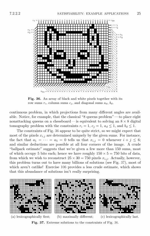
7.2.2.2 SATISFIABILITY: EXAMPLE APPLICATIONS 252 2 2 10 8 10 4 6 9 7 5 7 6 8 5 7 4 6 7 6 6 11 5 7 6 8 7 7 2 2

3

0

0

0

0

0

1

3

2

2

3

3

3

1

4

3

3

4

5

3

5

5

6

3

8

5

1

5

5

12

10

6

6

3

3

3

2

8

6

12

12

5

10

11

4

12

7

14

11

4

10

3 2 4 5 7 7 7 7 7 4 4 4 4 4 4 6 5 6 4 5 5 4 1 1 0 0 0 0 0

0

0

0

0

0

0

1

2

3

1

2

3

4

3

5

5

3

3

2

4

5

4

4

6

9834247767116645764645100000000

c1 = = c30

a1 =

a2 =

= r1= r2

= b1= b2

b54 =

= a54

Fig. 36. An array of black and white pixels together with itsrow sums ri, column sums cj , and diagonal sums ad, bd.

continuous problem, in which projections from many different angles are avail-able. Notice, for example, that the classical “8 queens problem” — to place eightnonattacking queens on a chessboard — is equivalent to solving an 8× 8 digitaltomography problem with the constraints ri = 1, cj = 1, ad ≤ 1, and bd ≤ 1.

The constraints of Fig. 36 appear to be quite strict, so we might expect thatmost of the pixels xi,j are determined uniquely by the given sums. For instance,the fact that a1 = · · · = a5 = 0 tells us that xi,j = 0 whenever i + j ≤ 6;and similar deductions are possible at all four corners of the image. A crude“ballpark estimate” suggests that we’re given a few more than 150 sums, mostof which occupy 5 bits each; hence we have roughly 150× 5 = 750 bits of data,from which we wish to reconstruct 25× 30 = 750 pixels xi,j . Actually, however,this problem turns out to have many billions of solutions (see Fig. 37), most ofwhich aren’t catlike! Exercise 106 provides a less crude estimate, which showsthat this abundance of solutions isn’t really surprising.

(a) lexicographically first; (b) maximally different; (c) lexicographically last.

Fig. 37. Extreme solutions to the constraints of Fig. 36.

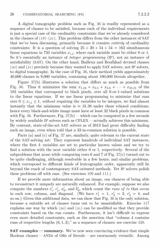
26 COMBINATORIAL SEARCHING (F6) 7.2.2.2

A digital tomography problem such as Fig. 36 is readily represented as asequence of clauses to be satisfied, because each of the individual requirementsis just a special case of the cardinality constraints that we’ve already consideredin the clauses of (18)–(21). This problem differs from the other instances of SATthat we’ve been discussing, primarily because it consists entirely of cardinalityconstraints: It is a question of solving 25 + 30 + 54 + 54 = 163 simultaneouslinear equations in 750 variables xi,j , where each variable must be either 0 or 1.So it’s essentially an instance of integer programming (IP), not an instance ofsatisfiability (SAT). On the other hand, Bailleux and Boufkhad devised clauses(20) and (21) precisely because they wanted to apply SAT solvers, not IP solvers,to digital tomography. In the case of Fig. 36, their method yields approximately40,000 clauses in 9,000 variables, containing about 100,000 literals altogether.

Figure 37(b) illustrates a solution that differs as much as possible fromFig. 36. Thus it minimizes the sum x1,24 + x2,5 + x2,6 + · · · + x25,21 of the182 variables that correspond to black pixels, over all 0-or-1-valued solutionsto the linear equations. If we use linear programming to minimize that sumover 0 ≤ xi,j ≤ 1, without requiring the variables to be integers, we find almostinstantly that the minimum value is ≈ 31.38 under these relaxed conditions;hence every black-and-white image must have at least 32 black pixels in commonwith Fig. 36. Furthermore, Fig. 37(b) — which can be computed in a few secondsby widely available IP solvers such as CPLEX — actually achieves this minimum.By contrast, state-of-the-art SAT solvers as of 2013 had great difficulty findingsuch an image, even when told that a 32-in-common solution is possible.

Parts (a) and (c) of Fig. 37 are, similarly, quite relevant to the current stateof the SAT-solving art: They represent hundreds of individual SAT instances,where the first k variables are set to particular known values and we try tofind a solution with the next variable either 0 or 1, respectively. Several of thesubproblems that arose while computing rows 6 and 7 of Fig. 37(c) turned out tobe quite challenging, although resolvable in a few hours; and similar problems,which correspond to different kinds of lexicographic order, apparently still liebeyond the reach of contemporary SAT-oriented methods. Yet IP solvers polishthese problems off with ease. (See exercises 109 and 111.)

If we provide more information about an image, our chances of being ableto reconstruct it uniquely are naturally enhanced. For example, suppose we alsocompute the numbers r′i, c′j , a′d, and b′d, which count the runs of 1s that occurin each row, column, and diagonal. (We have r′1 = 1, r′2 = 2, r′3 = 4, andso on.) Given this additional data, we can show that Fig. 36 is the only solution,because a suitable set of clauses turns out to be unsatisfiable. Exercise 117explains one way by which (20) and (21) can be modified so that they provideconstraints based on the run counts. Furthermore, it isn’t difficult to expresseven more detailed constraints, such as the assertion that “column 4 containsruns of respective lengths (6, 1, 3),” as a sequence of clauses; see exercise 438.

SAT examples — summary. We’ve now seen convincing evidence that simpleBoolean clauses — ANDs of ORs of literals — are enormously versatile. Among

INDEX AND GLOSSARYThe republic of letters is at present divided into three classes.

One writer, for instance, excels at a plan or a title-page,another works away the body of the book,

and a third is a dab at an index.— OLIVER GOLDSMITH, in The Bee (1759)

When an index entry refers to a page containing a relevant exercise, see also the answer tothat exercise for further information. An answer page is not indexed here unless it refers to atopic not included in the statement of the exercise.

∂S (boundary set), 58, 154, 180, 188.0–1 matrices, 106–109, 151, 176–177, 181,

see also Grid patterns.1SAT, 49, 148.2-colorability of hypergraphs, 185.2SAT, 49, 51–54, 77–78, 80, 101, 144,

147, 149, 157, 159, 266.3-regular graphs, 147, 154, 231.3CNF, 3, 148.3D MATCHING problem, 134, 225, 290–291.3D visualizations, 116–118.3SAT, 3–4, 47–51, 59, 60, 78–80, 93–94, 131,

135, 146, 148–151, 153, 182–184, 231.4-cycles, 109–110, 178, 225, 274.4-regular graphs, 290.4SAT, 49, 51, 150, 290.5SAT, 51, 58, 224, 291.6SAT, 51.7SAT, 51, 151.8 queens problem, 25, 282.90-rotational symmetry, 138, 202, 275.100 test cases, 113–124, 127, 182, 184.∅ (the empty set), 185.ϵ (the empty clause), 3, 27, 185, 291.ϵ (the empty string), 3, 85.ϵ (the tolerance for convergence), 93–94.ε (offset in heuristic scores), 126, 213.νx (1s count), see Sideways sum.π (circle ratio), see Pi.ρ (damping factor for variable activity),

67, 125–127, 155, 286.ρ (damping factor for reinforcement), 93–94.ϱ (damping factor for clause activity),

74, 125–127, 286.τ parameter, 125–127, 235, 286.τ(a, b) function, 147.ϕ (golden ratio), 146, 147, 160, 251.ψ (agility threshold), 76–77, 124–127,

240, 286.ψ (confidence level), 93, 255.

a.s.: almost surely, 149, 153.AAAI: American Association for Artificial

Intelligence (founded in 1979);

Association for the Advancement ofArtificial Intelligence (since 2007), 67.

Absorbed clauses, 168.Accordion solitaire, 282.Achlioptas, Dimitris (Aqliìptac,

Dhmătrhc), 221.ACT(c), 74, 125.ACT(k), 66–68, 75, 125, 132.Active path, 13.Active ring, 32.Activity scores, 67, 74–76, 125, 132,

155, 239.Acyclic orientation, 161.Adams, Douglas Noel (42), 126.Adaptive control, 46, 126.Addition, encoding of, 100–101, 114; see

also Full adders, Half adders.Adjacency matrix, 281.Adjacent pairs of letters, avoiding, 248.AGILITY, 76, 158, 240.Agility level, 76, 124, 158.Agility threshold (ψ), 76–77, 124–127,

240, 286.Ahmed, Tanbir (t;nbIr a;hemd), 5, 147.Alava, Mikko Juhani, 80.Aldous, David John, 219.Algorithm L0, 39, 147.Alice, 20–24, 139–141.All-different constraint, 171.All solutions, 143, 266.Alon, Noga (OEL@ DBEP), 174, 254, 260.Aloul, Fadi Ahmed (¿Ø£nň£m ŃÌČc ÝŁnş),

112, 281, 284.Analysis of algorithms, 146–152,

158–160, 164.Ancestors, 43.AND operation, 9, 10, 13.

bitwise (x & y), 28, 29, 31, 37, 38, 66, 68,76, 81, 196, 209–211, 220, 241.

André, Pascal, 131.Anisimov, Anatoly Vasilievich (Anisimov,

Anatoliȷ Vasil~eviq), 249.Annexstein, Fred Saul, 273.Anti-maximal-element clauses, 56, 62, 97,

115, 153, 155, 157, 167.

293

294 INDEX AND GLOSSARY

Antisymmetry, 178.Appier dit Hanzelet, Jean, 57.April Fool, 7.Ardila Mantilla, Federico, 256.Arithmetic progressions, 4, 114.

avoiding, 135.Armies of queens, 180.Asín Achá, Roberto Javier, 267.Asserting clause, see Forcing clause.Associative block design, 4.Associative law, 227.Asymmetric Boolean functions, 178.Asymmetric elimination, 260.Asymmetric tautology, see Certifiable

clauses.Asymptotic methods, 53–54, 147–151,

164, 210, 226, 230, 283.At-least-one constraint, 171, 265.At-most-one constraint, 6, 97–99, 103,

104, 120, 134, 149, 170, 171, 238,265, 266, 289.

ATPG: Automatic test pattern generation,see Fault testing.

Atserias, Albert Perí, 262.Audemard, Gilles, 72.Aurifeuille, Léon François Antoine,

factors, 14.Autarkies, 44, 71, 146, 152, 177, 214,

215, 217.testing for, 146, 214.

Autarky principle, 44.Automatic test pattern generation, see

Fault testing.Automaton, 272.Automorphisms, 108, 111, 180, 197,

236, 277.Autosifting, 220.Auxiliary variables, 6, 8, 15, 17, 60, 97, 101,

104, 105, 109, 135, 136, 148, 170–174,186, 262, 268, 276–279, 280–281, 287.

AVAIL stack, 257.Averages, 120.Avoiding submatrices, 106–107.Awkward trees, 227.Axiom clauses, 54, 59, 100, 264, 266.

Bacchus, Fahiem, 73, 271.Backjumping, 64, 68, 74, 132, 233, 236, 239.Backtrack trees, see Search trees.Backtracking, 4, 27–34, 38–39, 64, 105,

128, 129, 132, 151, 176, 190, 204,219, 231, 236.

Bailleux, Olivier, 8, 26, 135, 137, 143,174, 272.

Baker, Andrew Baer, 98.Balas, Egon, 206.Baldassi, Carlo, 93.Ball, Walter William Rouse, 180.Ballot numbers, 78.

Balls and urns, 221.Banbara, Mutsunori ( ), 264,

267, 268.Bartley, William Warren, III, 129.Basket weavers, 141.Batcher, Kenneth Edward, 266.Baumert, Leonard Daniel, 265.Bayardo, Roberto Xavier, Jr., 132.Bayes, Thomas, networks, 95.BCP: Boolean constraint propagation,

see Unit propagation.BDD: A reduced, ordered binary decision

diagram, 17–18, 102, 103, 132, 137, 148,174, 181, 188, 193, 194, 197, 202, 220.

BDD base, 219.Belief propagation, 95.Ben-Dor, Amir (XEC-OA XIN@), 289.Ben-Sasson, Eli (OEYY -OA IL@), 57–58,

153, 231.Benchmark tests, 35, 131–133, 139,

147, 190, 206.100 test cases, iv, 113–124, 127, 182, 184.

Bender, Edward Anton, 250.Beresin, May, 275.Berghammer, Rudolf, 204.BerkMin solver, 132.Berlekamp, Elwyn Ralph, 17.Berman, Piotr, 224.Bernhart, Frank Reiff, 188.Bernoulli, Jacques (= Jakob = James),

distribution, multivariate, 89.Bethe, Hans Albrecht, 95.Better reasons, 157.Bias messages, 92.Biased random bits, 12, 241.Biere, Armin, v, 66, 76, 96, 129, 132, 166,

188, 258, 260, 261, 269, 280.Big clauses, 145.BIMP tables, 36–41, 43, 45, 124, 144, 235.Binary addition, 114.Binary clauses, 3, 6, 36, 124, 133, 155–156.Binary constraints, 171.Binary decoder, 179.Binary implication graph, see Dependency

digraph, 41.Binary matrices, 106–109, 151, 176–177,

181, see also Grid patterns.Binary multiplication, 8.Binary number system, 9, 98.Binary recurrence relations, 189.Binary relations, 56.Binary search, 187.Binary strings, 181.Binary tensor contingency problem,

142, 151.Binomial coefficients, 149.Binomial convolutions, 250.Bipartite graphs, 58, 177, 290.Bipartite matching, 150.Bipartite structure, 90.

INDEX AND GLOSSARY 295

Birthday paradox, 49.Bishops, 141.Bitmaps, 17, 139.Bitwise operations, 11, 12, 81, 158, 161,

241, 246, 258–259.Black and blue principle, 146, 216.Black and white principle, 146.Blake, Archie, 130.blit, 234, 236.Block decomposition, 275.Block designs, 106.Block diagonal matrices, 177.Blocked clauses, 102, 215, 260, 261, 269.

binary, 146.elimination of, 167.

Blocked self-subsumption, 167.Blocking digraph, 215.Blocks in Life, 197, 200.Bloom, Burton Howard, coding, 258.Bloom, Thomas Frederick, 185.Bob, 20–24, 115, 139–141.Böhm, Max Joachim, 131.Bollobás, Béla, 54, 220.Bonacina, Maria Paola, 129.book graphs, 126, 179.Boole, George, 129.Boolean chains, 9, 11, 12, 102, 114, 173.

optimum, 178–179.Boolean formulas, 1.Boolean functions, 14–16.

expressible in kCNF, 220.synthesis of, 178–179.

Boppana, Ravi Babu, 174.Borgs, Christian, 54.Bottom-up algorithms, 252.Boufkhad, Yacine (ŃĹşØp ÑÛŞnÚ), 8, 26, 131,

135, 137, 143, 174, 272.Boundary sets, 58, 154, 180, 188.Boundary variables, 230.Bounded model checking, 16–24, 132,

137–141, 157, 179–180.Branching heuristics, 105, 144, see also

Decision literals.Branching programs, 102, 173, 174.Branchless computation, 242.Braunstein, Alfredo, 90, 91, 256.Breadth-first search, 37, 43, 68, 130, 235.Break count, 79.Breaking symmetries, vii, 5, 19, 105–114,

138, 176–181, 187, 188, 190–192, 238,267, 281–283, 285, 288–290.

in graph coloring, 99–100, 114, 171,179, 187.

Broadcasting, 170.Broadword computations, 11, 12, 158,

161, 246, 258.Brown, Cynthia Ann Blocher, 30, 32,

131, 151, 226.Brown, Thomas Craig, 185.

Brummayer, Robert Daniel, 269.Brunetti, Sara, 206.Bryant, Randal Everitt, v, 7, 187.BST(l), 211.BSTAMP counter, 211.Buckingham, David John, 197, 200.Buddy system, 36, 144, 235.Bugrara, Khaled Mohamed

(ÒŐmŔŕØpm ŃÌĎË Ń£nĞ), 226.Bugs, 16, 69, 77, 133, 240.Bulnes-Rozas, Juan Bautista, 215.Bumped processes, 21–22, 140, 202.Bundala, Daniel, 196.Burney, Charles, viii.Burns, James Edward, 204.Buro, Michael, 131.Buss, Samuel Rudolph, v, 153, 270.Bystanders, see Easy clauses.

C-SAT solver, 131.Cache memories, 24.Calabro, Chris, 288.Candidate variables, 40–44, 131, 214.Canonical forms, 138, 248.Cardinality constraints, 7–8, 26, 104, 106,

113, 114, 121, 135, 143, 187, 188,193, 194, 196, 204, 285.

for intervals, 100, 190, 280.Carlier, Jacques, 131.Carlitz, Leonard, 162.Carriers in Life, 197, 200.Carroll, Lewis (= Dodgson, Charles

Lutwidge), 129–130.Carry bits, 9, 12, 101, 192, 193.Cartier, Pierre Emile, 83, 86, 163.Case analysis, 27, 130.CDCL (conflict driven clause learning)

solvers, 62–71, 103, 121, 132–133, 155.combined with lookahead solvers, 129.compared to lookahead solvers, 98–100,

118–121, 182, 290.Cells of memory, 28, 122–124.Cellular automata, 17, 202.Certifiable clauses, 168, 260.Certificates of unsatisfiability, 69–71,

157, 169, 176, 178.Chaff solver, 67, 132.Chain rule for conditional probability, 254.Chains, 276, see also Boolean chains,

Resolution chains, s-chains.Channel assignment, 136.Channeling clauses, 264.Characteristic polynomial of a matrix,

163, 218.Chavas, Joël, 91.Chayes, Jennifer Tour, 54.

296 INDEX AND GLOSSARY

Chebyshev (= Tschebyscheff), PafnutiiLvovich (Qebyxev­, Pafnut˛ȷL~voviq­ = Qebyxev, PafnutiȷL~voviq), inequality, 221.

polynomials, 247.Cheshire Tom, 24–26, 115, 142–143.Chess, 7, 170.Chessboards, 18, 25, 99, 106, 115, 138, 180.Chiral symmetry (rotation but not

reflection), 138, 202, 275.Chordal graphs, 163–164.Chromatic number χ(G), 99, 135–136,

147, 174, 281.Chung Graham, Fan Rong King

( ), 283.Chvátal, Václav (= Vašek), 5, 52, 59, 185.Cimatti, Alessandro, 132.Circuits, Boolean, 10, 101–103, 114, see

also Boolean chains.Circular lists, 32.Clarke, Edmund Melson, Jr., 132.Clashing pairs of letters, 84.Clausal proofs, see Certificates of

unsatisfiability.Clause activity scores, 74, 239.Clause-learning algorithms, 61–62, 103,

118, 121, 132–133, 154–155.Clauses per literal, 150, 231; see also

Density of clauses.Claw graph, 249.Clichés, 76.Clique Local Lemma, 165.Cliques, 81, 100, 162, 167, 169, 171,

179, 190.covering by, 165.

Closest strings, 114, 181, 182.Clusters, 166.CNF: Conjunctive normal form, 9, 101,

154, 173, 193, 196.Cocomparability graphs, 249, 250.Coe, Timothy Vance, 201.Coexisting armies of queens, 180.Cographs, 163, 250.Cohen, Bram, 79, 246.Coja-Oghlan, Amin, 221.Colexicographic order, 206, 278.Coloring a graph, 6–7, 99–100, 153, 179, 260.

fractional, 135.multiple, 135.of queens, 99–100, 114–115, 171.radio, 136.

Column sums, 151.Commutative law, 27, 180, 227.

partial, 83, 250–251.Comparator modules, 115, 137.Comparison, lexicographic, 101, 111–113.Comparison of running times, 34–35, 39,

69, 97–100, 105–107, 110, 112, 118–128,182, 184, 218, 237, 264, 281, 290.

Compensation resolvents, 39, 144, 147.Competitions, 131–133, 291.Complement of a graph, 134.Complementation of unary representations,

100.Complemented literals, 2–4, 37, 62–64,

78, 111, 210, 266.Complete binary trees, 8, 135, 230.Complete bipartite graphs Km,n, 250, 254.Complete graphs Kn, 153, 178, 186, 262.Complete k-partite graphs, 250, 262.Complete t-ary trees, 160.Compressing, see Purging unhelpful clauses.Conditional autarkies, 215.Conditional expectation inequality, 150.Conditional symmetries, 107, see

Endomorphisms.Conditioning operations (F | l and F |L), 27,

96, 143, 157, see Unit conditioning.Cones in trace theory, 87.Confidence level (ψ), 93, 255.Conflict clauses, 63, 70, 171; see also

Preclusion clauses.Conflict driven clause learning, 62–69,

103, 121, 132–133, 155.Conflicts, 62, 124, 132.Conjunctive normal form, 1, 9, 101,

154, 173, 193, 196.irredundant, 257.

Conjunctive prime form, 104.Connected graphs, 177.Connectedness testing, 169–170.Connection puzzles, 170.CoNP-complete problems, 3, 207.Consecutive 1s, 88, 175, 254.Consensus of implicants, 130.Consistent Boolean formulas, see

Satisfiable formulas.Consistent partial assignments, 30, 165.Constrained variables in partial assignments,

165–166.Contests, 131–132.Context free languages, 175.Contiguous United States, 136.Contingency tables, binary, 142.

3D, 151.Convex functions, 216.Convex hulls, 247.Convolution principle, 250.Conway, John Horton, 17, 139, 201.Cook, Stephen Arthur, 61, 62, 130–131,

154, 229, 237.cook clauses, 157.Cooper, Alec Steven, 285.Core assignments, 166.Core of Horn clauses, 174, 216.Coupon collector’s test, 220.Covering assignments, 166, 221, 255.Covering problems, 2, 193, 194, see also

Domino coverings.

INDEX AND GLOSSARY 297

Covering strings, 181.CPLEX system, 26, 289.CPU: Central Processing Unit (one

computer thread), 121.Crawford, James Melton, Jr., 98, 113.Cray 2 computer, 137.Critical sections, 21–23, 140–141.Crossover point, see Threshold of

satisfiability.Crusoe (= Kreutznaer), Robinson, vii.CSP: The constraint satisfaction

problem, 283.Cube and conquer method, 129.Cubic graphs (3-regular, trivalent),

147, 154, 231.Cufflink pattern, 255.Culver, Clayton Lee, 185.Cut rule, 59.Cutoff parameters, 41, 145.Cutting planes, 184, 206.Cycle detection problem, 260.Cycle graphs Cn, 135, 160, 262.Cycle structure of a permutation, 108,

112–113, 163, 178, 277.Cyclic DPLL algorithm, 33.Cyclic patterns, 19.Cyclic permutations, 163.

da Vinci, Leonardo di ser Piero, 7.Dadda, Luigi, 9, 114, 136, 173.Dags: Directed acyclic graphs, 54.

of resolutions, 54–56, 70.Damping factors, 46, 67, 74, 76, 93–94,

125, 126, 155.Dancing links, 5, 121, 134, 208, 288, 291.Dantchev, Stefan Stoyanov (Danqev,

Stefan Stofflnov), 110.Darwiche, Adnan Youssef

(ŹÚŒŐŁ ţŞØÚ ÎnÏŃń), 67, 262.Data structures, 28–34, 36–38, 43, 66–67,

80, 95–96, 143–145, 155–156, 159,167, 238, 273.

Davis, Martin David, 9, 31–32, 130, 298.Dawson, Thomas Rayner, 170.De Morgan, Augustus, laws, 3.de Vries, Sven, 206.de Wilde, Boris, 213.Deadlock, 22–23.Debugging, 69, 77.Dechter, Rina Kahana (XHKC @PDK DPIX), 67.Decision literals, 62, 69, 124, 132.Decision trees, see Search trees.Decomposable matrices, 177.Default parameters, 93, 125–126.Default values of gates, 11.Definite Horn clauses, 174.Defoe, Daniel (= Daniel Foe), vii.Degree of a vertex, 191.Degrees of truth, 37–39, 42–43, 45–46, 216.

Dekker, Theodorus Jozef, 140.Del Lungo, Alberto, 206.Delayer, 55–56, 152–153.Deletion from a heap, 234.Delta sequence, 290.Demenkov, Evgeny Alexandrovich

(Demenkov, Evgeniȷ Aleksandroviq),280.

Density of clauses: The number of clausesper variable, 50–51, 150, 231, 288.

Dependence graph in trace theory, 248.Dependence of literals, 63.Dependency digraph (of literals), 41, 131,

168, 215, 237, 260.Dependency-directed backtracking, see

Backjumping.Dependency graph (of events), 82, 164, 165.Dependency on a variable, 137.Depth-first search, 130.Dequen, Gilles Maurice Marceau, 131.Determinants, 162, 163, 251.Deterministic algorithm, 17, 120.Deventer, Mattijs Oskar van, 290.DFAIL, 46, 147.Dfalse literals, 45.Diagonals of a matrix, 24–25, 141–142.Diagram of a trace, 84.Díaz Cort, José Maria (= Josep), 51.Dick, William Brisbane, 180.Difficult instances of SAT, 5, 14, 26, 51,

55–59, 118–121, 153–154, 184, 190,192, 197, 206, 280.

Digital tomography, 24–26, 115, 141–143,167, 285.

Digraphs, 54, 108, 161, 162, 263, see alsoBlocking digraph, Dependency digraph,Implication digraph.

Dijkstra, Edsger Wybe, 22, 202, 204.DIMACS: Center for Discrete Mathematics

and Theoretical Computer Science, 131.DIMACS: DIMACS Series in Discrete

Mathematics and Theoretical ComputerScience, inaugurated in 1990.

Ding, Jian ( ), 51.Direct encoding, 98, 114, 171, 186,

264, 265, 281.Direct sum of graphs or matrices, 162, 177.Directed acyclic graphs of resolutions,

54–56, 70.Directed graphs, see Digraphs.Discarding the previous learned clause,

72, 156.Discrepancy patterns, 114, 182.Disjoint shortest paths, 276.Disjunctive normal forms, 14, 115,

130, 195, 257.Distance d(u, v) in a graph, 262.Distinct literals, 2.Division of traces, 85, 161, 250.

298 INDEX AND GLOSSARY

DNF: Disjunctive normal form, 14, 115,130, 195, 257.

Dodgson, Charles Lutwidge, 129–130.Domino coverings, 110, 114, 115, 143,

177, 178.Don’t-cares, 194, 280.Double clique hints, 100, 114, 171.Double coloring, 115, 135.Double lookahead, 45–46, 126, 131, 286.Double order, 214.Double truth, 45.Doubly linked lists, 28, 257, 259.Downhill resolution, 96, 166.Downhill transformations, 95.Doyle, Arthur Ignatius Conan, 72.DPLL (Davis, Putnam, Logemann,

Loveland) algorithm, 32–33, 62.with lookahead, 38, 131.

DT (double truth), 45.Dtrue literals, 45.Dual of a Boolean function, 130, 174.Dubois, Olivier, 131.Dudeney, Henry Ernest, 114, 263.Dufour, Mark, 37.Dull, Brutus Cyclops, 181.Durfee, William Pitt, square, 276.Dynamic storage allocation, 144.Dynamical system, discrete, 16.

e, as source of “random” data, 12, 193.Eager data structures, 30, 36, 156.Easy clauses, 149.Eaters in Life, 20, 139.Eén, Niklas Göran, v, 67, 96, 166,

203, 260, 268.Ehlers, Thorsten, 196.Eightfold symmetry, 138, 198.Elegance, 35–36, 196.Elimination of clauses, 167–168; see also

Purging unhelpful clauses.Elimination of variables, 60–61, 95–97, 101,

102, 129, 130, 154–155, 166–168, 173,174, 256–257, 259–260, 270, 271.

Embedded graphs, 169, 262.Empilements, 84, 161, 248.Empirical performance measurements,

122–124.Empty clause (ϵ), 3, 27, 185.Empty list, representation of, 33, 210.Empty partial assignment, 166.Empty set (∅), 185.Empty string (ϵ), 3, 85.Encoding into clauses, 6, 18, 97–105, 120,

134, 170, 179, 198, 202.ternary data, 100, 141, 179.

Endomorphisms, 107–111, 177–178,181, 281, 290.

Equal sums, encoding of, 174.Equally spaced 1s, 4, 114, 135; see

also waerden .

Equivalence classes in trace theory, 84.Equivalence of Boolean functions, 178.Erdős, Pál (= Paul), 81, 107, 190, 281.

discrepancy patterns, 114, 179, 182.Erp rules, 95–96, 166–168, 259.Evaluation of Boolean functions, 137,

178–179, 194.Even-length cycles, 277.Even-odd endomorphisms, 110, 177–178.Exact cover problems, vii, 2, 5–6, 28, 134,

183, 186, 219, 225, 257, 291.by pairs (perfect matchings), 109–110,

see also Domino coverings.by triples (3D MATCHING), 134,

225, 290–291.fractional, 135–136.

Exclusion clauses, 6, 21, 99, 114, 134,149, 153, 238, 260, 289.

Exclusive or, ternary, 136.Existential quantifiers, 60.Expander graphs, 58, 231.Exploitation stack, 259.Exploration phase of lookahead, 40, 43–44.Exponential time, 144.

hypothesis, 288.Extended resolution, 60, 71, 133, 154,

168, 215.Extreme distribution, 87, 89, 163.

factor fifo(m,n, z), 10, 12, 114, 184, 192.factor lifo(m,n, z), 10, 114, 184, 192.factor rand(m,n, z, s), 10, 184.Factorization, 8–10, 136, 184, 192.

of traces, 86, 162, 250.Failed literals, 97, 167, 175, 269.Fallacious reasoning, 16, 284.False hits, 258.False literals preferred, 31, 33, 67,

125–127, 286.Fanout gates, 10–14, 136.Fat clauses, 58.Fault testing, 10–14, 114, 126, 136–137,

167, 260.Feedback mechanism, 46, 104.Fermat, Pierre de, 10.Fernandez de la Vega, Wenceslas, 52.Fibonacci, Leonardo, of Pisa (= Leonardo

filio Bonacii Pisano), numbers,160, 215, 254.

ruler function, 246.Fichte, Johannes Klaus, 262.Field of a variable, 91, 165.FIFO: first in, first out, 10.Finite-state automata, 175.First in, first out, 10.First moment principle, 53, 148, 150.First order logic, 59, 130.Fischetti, Matteo, 206.Fixed point of endomorphisms, 177.

INDEX AND GLOSSARY 299

Fixed values of literals, 37, 42–46.FKG inequality, 89.Flag bits, 235.Flammenkamp, Achim, 198.Flexibility coefficients, 91.Flickering state variables, 141.Flipflops in Life, 138, 143.Floating point arithmetic, 91–92, 217, 239.

overflow, 67.Floor tiling, 115, 143, 199.Flower snarks, 69, 147, 153, 157.Flushing literals and restarting, 68, 75–77,

124, 132, 157, 158, 169, 234, 246.Foata, Dominique Cyprien, 83, 86, 163.Focus of attention, 41, 67, 91, 132.Foe, Daniel (= Daniel Defoe), vii.Footprint heuristic, 279.Forced literals, 45.Forcing clause, 62, see Unit propagation.Forcing representations, 104–105, 174,

175, 274.Forests, 43, 87, 163.Forgetting clauses, 168, 169, see Purging

unhelpful clauses.Four bit protocol, 115.Four Color Theorem, 7.Fourfold symmetry, 138.Fractional coloring number, 135.Fractional exact cover, 135–136.Frances, Moti (QQPXT ICEN), 285.Franco, John Vincent, 131, 148, 225, 273.Free literals and free variables, 38,

66, 165–166.Freeman, Jon William, 131.Friedgut, Ehud (HEBCIXT CED@), 51.Frontier (∂in), 180, 188.Frost, Daniel Hunter, 67.fsnark clauses, 69, 71, 114, 147–148,

153, 157.Full adders, 9, 136, 179, 192, 268, 278.

modified, 114, 280.Full runs, 73, 158, 235.Furtlehner, Cyril, 91.

Gµ: Gigamems = billions of memoryaccesses, 97, 118.

per minute, 289.Gadgets, 134, 183.Gallager, Robert Gray, 95.Game of Life, 17–20, 97, 114, 137–139,

143, 167.Garden of Eden, 139.Gardner, Martin, 7, 19, 181, 188, 283.Gates, 10–13, 101–103, 121, 136.GB GATES, 13–14.Gebauer, Heidi Maria, 224.Geek art, 116–117.Generalization of resolution, 226.

Generating functions, 85, 89–90, 151,158–159, 164, 188, 194, 219, 222,230, 284.

exponential, 162.Generic graph, 174.Gent, Ian Philip, v, 265, 283.Gentzen, Gerhard Karl Erich, 59.Geometric distribution, 244, 262.Georges, John Pericles, 192.Gerdes, Paulus Pierre Joseph, 205.Gessel, Ira Martin, 248.Giant strong component, 52.Gigamem (Gµ): One billion memory

accesses, 35, 39, 97, 188.per minute, 289.

Ginsberg, Matthew Leigh, 113.Gipatsi patterns, 141.Girth of a graph, 176, 290.Given literals (F | l or F |L), 27, 96, 143,

157; see also Unit conditioning.Gliders in Life, 19, 138–139, 197, 201.

symmetry of, 200.Global ordering, 284.Glucose measure, see Literal block distance.Goerdt, Andreas, 52.Goldberg, Allen Terry, 131, 225.Goldberg, Eugene Isaacovich (Gol~dberg,

Evgeniȷ Isaakoviq), 70, 132.Goldman, Jay Robert, 250.Goldsmith, Oliver, 293.Golomb, Solomon Wolf, 265.González-Arce, Teófilo Francisco, 268.Gosper, Ralph William, Jr., 20, 198.Goultiaeva, Alexandra Borisovna

(Gul~tffleva, Aleksandra Borisovna),73.

Grabarchuk, Peter Serhiyevich (Grabarquk,Petro Serg˛ȷoviq), 263.

Grabarchuk, Serhiy Alexeevich (Grabarquk,Serg˛ȷ Oleks˛ȷoviq), 263.

Grabarchuk, Serhiy Serhiyevich (Grabarquk,Serg˛ȷ Serg˛ȷoviq), 263.

Graham, Ronald Lewis ( ), 185, 283.Graph-based axioms, 59, 154, 178, 290.Graph coloring problems, see Coloring

a graph.Graph embedding, 169, 262.Graph layout, 116–118.Graph quenching, 114, 179–180, 281.Gray, Frank, codes, 201, 282.Greedy algorithms, 80, 136, 172.Greenbaum, Steven Fine, 102.Greene, Curtis, 276.Grid graphs, 110, 136, 151, 162–163.

list coloring of, 151.Grid patterns, 17–20, 24–26, 137–139, 142.

rotated 45, 141–142.Griggs, Jerrold Robinson, 192.Grinbergs, Emanuels Donats Frıdrihs

Jänis, 218.

300 INDEX AND GLOSSARY

Gritzman, Peter, 206.Grötschel, Martin, 264.Gu, Jun ( ), 77.Guéret-Jussien, Christelle, 267.Guilherme De Carvalho Resende,

Mauricio, 16.GUROBI system, 289.Guy, Richard Kenneth, 17, 19, 107.Gwynne, Matthew Simon, 105, 270, 273.

Hackers, 199.Haken, Armin, 57, 58.Halevi, Shai (IELD IY), 289.Half adders, 9, 192, 268.Halting problem, 130.Hamadi, Youssef (âamady ľuÓaf, ÝŁnÌČ

ţŞØÚ), 236.Hamilton, William Rowan, cycles, 169.

paths, 184.Hamming, Richard Wesley, distance, 285.Han, Hyojung ( ), 236.Handwaving, 89.Hanzelet, see Appier dit Hanzelet.Hard clauses, 168.Hard sudoku, 183.Hartman, Christiaan, 202.Haven, G Neil, 131.Head of the list, 28.Header elements, 225.HEAP array, 67, 158, 233–235, 240.Heap data structure, 67, 214.

insertion and deletion from, 234.Heaps of pieces, 83.Height of a literal, 214.Height of a trace, 85.Heilmann, Ole Jan, 251.Helpful rounds, 169.Heule, Marienus (= Marijn) Johannes

Hendrikus, v, 37, 40, 46, 71, 75, 97–98,104, 129, 134, 147, 182, 186, 202,213, 239, 260, 261, 263.

Heuristic scores, 90–95.for clauses, 72–74, 125–127, 158, 239, 286.for variables, 40–44, 61, 67, 80, 126,

145–147, 214.Hidden weighted bit function, 173.Hierarchy of hardness, 176, 178.Hilton, Anthony John William, 191.Hint clauses, 100, 114, 171.Hirsch, Edward Alekseevich (Girx, ˜duard

Alekseeviq), 215.Historical notes, 32, 59–60, 105,

129–133, 231.Hollow mazes, 290.Holmes, Thomas Sherlock Scott, 72.Homomorphic embedding, 169, 262.Honest representations, 105, 270.Hoory, Shlomo (IXEG DNLY), 224.Hoos, Holger Hendrik, v, 125–127, 133, 160.

Horn, Alfred, clauses, 132, 166, 176,216, 263.

core of, 174, 216.renamed, 176, 263.

Horsley, Daniel James, 274.Horton, Robert Elmer, numbers, 152.Hsiang, Jieh ( ), 129.Hume, David, 1.Hunt, Warren Alva, Jr., 71, 239.Hutter, Frank Roman, 125, 133.Hypergraph 2-colorability, 185.Hyperresolution, 56, 228, 257.

Idle Year solitaire, 180.IEEE Transactions, vi.If-then-else operation (u? v: w), 81,

102, 152, 173, 219.ILS: Iterated Local search, 125.Impagliazzo, Russell Graham, 55, 288.Implication digraph, 52, 144.in situ deletion, 156.Inclusion and exclusion, 221–222, 256.Inconsistent clauses, see Unsatisfiable

formulas.Indecomposable matrices, 177.Independent vertices, 7, 147.Induced graph, 262.Induction proofs by machine, 24, 203.Infinite loop, 244.Initial guess for literals, 31, 33, 66,

125–127, 286.Initial state X0, 16–17, 21, 24, 140, 202.Inprocessing, 95, 168.Input and output, 120.Input states, 175.Insertion into a heap, 234.Integer programming, 26, 184, 206, 285.Interactive SAT solving, 142.Interlaced roots of polynomials, 163.Internet, ii, iv, v, 118.Intersection graphs, 84, 161.Interval graphs, 87, 163.Intervals, cardinality constrained to,

100, 190, 280.Invariant assertions, 23–24, 43, 115, 140,

203, 216, 217, 255, 261.Inverse permutations, 112, 265.Inversions of a permutation, 213.Involution polynomial of a set, 163.Involutions, signed, 112–113, 180, 277–278.INX array, 38, 211, 286.IP: Integer programming, 26, 184, 206, 285.Irredundant CNF, 257.Irreflexive relation, 56.Irving, Robert Wylie, 151.Isaacs, Rufus Philip, 218.Isolated vertices, 262.IST array, 38.ISTACK array, 38, 145.ISTAMP counter, 37–38, 46, 145.

INDEX AND GLOSSARY 301

Iterated local search, 125.Iwama, Kazuo ( ), 224.

Jabbour, Saïd (jabur Óayd, ŐØq~ ŃÛňŞ),236, 289.

Jacquet, Philippe Pierre, 225.Jagger, Michael Philip “Mick”, 1.Janson, Carl Svante, v.Järvisalo, Matti Juhani, 105, 132, 260, 261.Jeannicot, Serge, 215.Jeavons, Peter George, v.Jerrum, Mark Richard, 151.Job shop problems, 172.Johnson, David Stifler, 184, 191.Johnson, Samuel, viii.Join of graphs, 162.

k-induction, 203.Kµ: Kilomems = thousands of memory

accesses, 98.Km,n (complete bipartite graph), 176.Kamath, Anil Prabhakar (aEnl þBAkr

kAmT), 16.Kaporis, Alexis Constantine Flora (Kapìrhc,

Alèxioc KwnstantÐnou Flÿrac), 51.Karmarkar, Narendra Krishna (nr˚dý

k¯Z krmrkr), 16.Karp, Richard Manning, 52, 268.Karpiński (= Karpinski), Marek

Mieczysław, 224.Karpovsky, Mark Girsh, 285.Kasif, Simon (SIQK OERNY), 265.Katona, Gyula (Optimális Halmaz), 107.Kautz, Henry Alexander, 79, 132.Kaye, Richard William, 207.Keller, Robert Marion, 83.Kernel of a graph, 99, 134, 186, 188, 218.

clauses for, 114, 134.Kilomem (Kµ): One thousand memory

accesses, 39, 98.Kim, Jeong Han ( ), 54.King moves, 134, 169.Kingwise connected cells, 170.Kirousis, Lefteris Miltiades (KuroÔshc,

Eleujèrioc MiltiĹdhc), 51.Kitagawa, Satoshi ( ), 264, 267.Kleine Büning (= Kleine-Büning), Hans

Gerhard, 131, 185.Kleitman, Daniel J (Isaiah Solomon), 276.Knapsack problem with a partial

ordering, 158.Knessl, Charles, 225.Knight moves, 115, 169.Knuth, Donald Ervin ( ), i, ii, v,

1, 14, 16, 19, 51–52, 72, 74, 93, 94,118, 125–127, 192, 193, 195, 197,202, 210, 212, 213, 216, 227, 235–237,240, 242, 249, 260, 264–267, 274,278, 279, 282, 286, 290.

Knuth, John Martin ( ), see Truth.Kojevnikov, Arist Alexandrovich

(Koıevnikov, Arist Aleksandroviq),280.

Kolipaka, Kashyap Babu Rao (GŘÞĄľ ĂG ĂGĂlő Ťa

cĄcĞ gĄkĂÒ), 90, 161, 255.Konev, Boris Yurevich (Konev, Boris

“r~eviq), 281.Kouřil, Michal, 5, 185.Kroening, Daniel Heinrich Friedrich

Emil, v, 203, 288.Krom, Melven Robert, clauses, see 2SAT.kSAT, 3, 49–51, 146, 148, 150, 183.Kulikov, Alexander Sergeevich (Kulikov,

Aleksandr Sergeeviq), 280.Kullmann, Oliver, v, 5, 105, 129, 147, 152,

215, 216, 218, 228, 260, 270, 273.Kwekkeboom, Cornelis (= Kees)

Samuël, 202.

L(2, 1) labeling of graphs, 136.L7 lattice, 255.Labeled pyramids, 162.Labeled traces, 162.Lalas, Efthimios George (LĹlac, EujÔmioc

GewrgÐou), 51.Lamport, Leslie B., 24, 204.Land mines, 142.Landman, Bruce Michael, 185.Langford, Charles Dudley, problem of

pairs, vii, 5–6, 34, 98, 121, 125,134, 170, 186, 289.

langford(n), 6, 34–35, 39, 97, 98, 114,121, 134, 210, 236, 289.

langford ′(n), 6, 98, 114, 134, 289.langford ′′(n), 98.langford ′′′(n), 264.Larrabee, Tracy Lynn, 13, 137.Las Vegas algorithms, iv, 159–160.Last in, first out, 10.Late Binding Solitaire, 114, 180.Latin rectangle construction, 151.Lattices, 255, 276.

of partial assignments, 165–166.Lauria, Massimo, v, 56.Laurier, Jean-Louis, 187.Lazy data structures, 30–34, 36, 65,

156, 234.Le Berre, Daniel Claude Yves, 132.Learned clauses, 63–65, 70–71, 124, 132, 168.

sequence of, 70, 156.Learning a Boolean function, 14–16,

115, 137.Least common ancestor, 253.Left division of traces, 85, 161.Left factor of a trace, 161–162.Lemaire, Bernard François Camille, 282.Lemma generation, see Clause-learning

algorithms.Length of a trace, 85.

302 INDEX AND GLOSSARY

Lettmann, Theodor August, 185.Level 0, 62, 66, 124, 156, 207, 233.Levels of values, 62–66, 156, 233.Levesque, Hector Joseph, 50.Levine, Eugene, 275.Lewis, Jerome Luther, 275.Lex-leader: The lexicographically smallest

element, 111, 283.Lexicographic order, 4, 25, 26, 30, 101, 105,

107, 109, 111–113, 115, 197, 282–283.encoded in clauses, 101, 173, 174.

Lexicographic row/column symmetry,106–107, 177, 181, 274.

Lexicographically smallest (or largest)solution, 25–26, 111–113, 142,157, 282, 283.

Lexicographically smallest traces, 84,161, 162, 250.

Leyton-Brown, Kevin Eric, 125, 133.Li, Chu Min ( ), 131.Li, Wei ( ), 149.Lieb, Elliott Hershel, 251.Life, Game of, 17–20, 97, 114, 137–139,

143, 167.Light speed in Life, 139.Line graph of a graph, 147, 249.Linear equations, 26, 231.Linear extensions, see Topological sorting.Linear inequalities, 184.

encoding of, 100–101, 172, 173.Linear programming relaxation, 26.Lines, abstracted, 106.Links, dancing, 5, 121, 134, 208, 288.Lisitsa, Alexei Petrovich (L˛s˛ca, Alfflkseȷ

Pffltrov˛q), 281.List coloring of graphs, 135, 151.List merging, 231, 258.Literal block distance, 72, 74, 158.Literals, 2, 111.

flushing, 76.internal representation, 28, 37, 66,

208, 209, 242, 257.Litman, Ami (ONHIL INR), 285.Livelock, 22–23.Llunell, Albert Oliveras i, 267.LNCS: Lecture Notes in Computer Science,

inaugurated in 1973.Local Lemma, 81–90, 133, 151, 160–165.Log encodings, 98, 114–115, 173.Logemann, George Wahl, 31–32, 130, 298.Longest simple path, 23, 203.Lonlac, Jerry, 289.Look-back, see Backjumping.Lookahead autarky clauses, see Black

and blue principle.Lookahead forest, 42–44, 145–147, 168.Lookahead solvers, 38–46, 55, 97, 129,

131, 176.combined with CDCL solvers, 129.

compared to CDCL solvers, 98–100,118–121, 182, 290.

Loopless shadows, 184.Lopsidependency graphs, 82, 83, 160,

164, 165, 185, 224.Lovász, László, 81, 82, 185, 191.Loveland, Donald William, 32, 130, 298.Lower semimodular lattices, 255–256.Loyd, Samuel, 263.Luby, Michael George, 80, 159.Luks, Eugene Michael, 113.

Mµ: Megamems = millions of memoryaccesses, 69, 98.

Maaren, Hans van, 37, 46.MacColl (= McColl), Hugh, 227.MacMahon, Percy Alexander, Master

Theorem, 250, 251.Mader, Adolf, 275.Madigan, Conor Francis, 132.Magic, 193.Magic sequences, 285.Magnetic tape, 32.Makespan, 172–173.Mallach, Sven, 289.Malik, Sharad (frd mElk), 132.Maneva, Elitza Nikolaeva (Maneva, Elica

Nikolaeva), 166, 256.Mapping three items into two-bit codes, 179.march solver, 40, 216.Marek, Victor Wiktor, 216.Markov (= Markoff), Andrei Andreevich

(Markov, Andreȷ Andreeviq), theelder, inequality, 158, 241.

Markov, Igor Leonidovich (Markov, ¨gorLeon˛doviq), 112, 281, 284.

Markström, Klas Jonas, 290.Marques da Silva (= Marques-Silva),

João Paulo, 132.Marriage theorem, 224.Martin, Alexander, 264.Matching polynomial of a graph, 249.Matchings in a graph: Sets of disjoint

edges, 150, 230, 249.perfect, 109–110, 177.

Mathews, Edwin Lee (41), 67.Matrix multiplication, 260.Matroids, 276.Mauro, David Whittlesey, 192.Maximal elements, 56, 62, 97, 115,

153, 157, 167.Maximal planar graphs, 186.Maximum independent sets, 87, 136,

187, 188.Maximum number of 1s, 106–109,

135, 136, 177.MAXSAT lower bound, 184.“Maybe” state, 20.Mazurkiewicz, Antoni Wiesław, 83.McColl (= MacColl), Hugh, 227.

INDEX AND GLOSSARY 303

McGregor, William Charles, 7, 188.graphs, 7–8, 114–115, 134, 135, 188.

Mean running time, 120.Median operation, 9, 136, 179.Median running times, 99, 120–124, 127.Megamem (Mµ): One million memory

accesses, 201.Méjean, Henri-Michel, 226.Mellin, Robert Hjalmar, transforms, 151.Mem (µ): One 64-bit memory access, 34.MEM array, 66, 68, 124, 156.Memo cache, 60, 233.Memoization technique, 233.Memoryless property, 244.Menagerie, 116–117.Merge networks, 266.Merging lists, 231, 258.Mertens, Stephan, 51.Message passing, 90–95, 165–166.Method I, 61.Method IA, 61, 154.Method of Trees, 129.Methuselah solitaire, 282.Methuselahs in Life, 19.Mézard, Marc Jean Marcel, 51, 90, 91, 95.Midpoint inequalities, 266.Mijnders, Sid, 213.Mills, Burton Everett, 130.Minesweeper, 142–143.Minimally unsatisfiable clauses, 150, 153.Minimum covers, 193.MiniSAT, 67.Minterms, 179.Mitchell, David Geoffrey, 50.Miters, 121, 182.Mitsche, Dieter Wilhelm, 51.Mixed metaphors, 76.Mixed-radix number systems, 268.MMIX computer, ii, 158.Mobile Life paths, 18–19, 138–139.

flipflops, 138.Möbius, Augustus Ferdinand, functions, 86.

series, 86, 160, 162–163, 165, 247, 249.Mod 3 addition, 114, 179.Mod 3 parity, 179.Mod 4 parity, 179.Model checking, 16–17, 137–141, 179–180.Model RB, 149.Modified full adders, 114, 280.Modular lattices, 255.mone (−1), 242.Monien, Burkhard, 215.Monkey wrench principle, 113, 181.Monotone functions, 163.

Boolean, 137, 281.Monotonic clauses, 5, 133, 157.Monotonic paths, 108, 276.Montanari, Andrea, 95.Monte Carlo algorithms, iv, 77–83, 158–160.

Monus operation (x .−y = max0, x−y),vi, 92, 247, 268.

Moore, Edward Forrest, 202.Morehead, Albert Hodges, 282.Morel, Henri, 226.Moser, Robin Alexander, 82, 254.Moskewicz, Matthew Walter, 132.Mossel, Elchanan (LQEN OPGL@), 166.Mott-Smith, Geoffrey Arthur, 282.Move codes, 29–31, 34, 144, 145, 155, 210.MPR: Mathematical Preliminaries Redux, v.Mueller, Rolf Karl, 60, 130.Müller, Mike, 196.Multicommodity flows, 170.Multigraphs, 231.Multilinear function, 86.Multiplication of binary numbers, 8–9,

12–14, 114, 136, 173.Multiplication of traces, 85, 161.Multisets, 3, 214, 224, 250.Multivalued graph colorings, 99.Mutilated chessboard, 110, 114,

177–178, 286.Mutual exclusion protocols, 20–24,

115, 139–141.Mutzbauer, Otto, 275.Mux operation (u? v: w), 81, 102,

152, 173, 219.Mysterians, 290.

n-cube, 79, 136, 148, 184.n.f.: not falsified, 271.n queens problem, 25, 115, 171, 282.NAND operation, 60.Napier, John, Laird of Merchiston, 9, 173.Near truth, 37–39.Necessary assignments, 45, 146.Negated auxiliary variables, 105.Negative k-clauses, 157.Negative literals, 2, 132, 153.Nesting phase of lookahead, 40, 42–43,

145–147.Newbie variables, 41.Newton, Isaac, method for rootfinding,

216–217.Niborski, Rodolfo, 190.Niemelä, Ilkka Niilo Fredrik, 105.Nieuwenhuis, Robert Lukas Mario, 267.Nightingale, Peter William, 265.No-player game, 17.Nodes of a search tree, 34–35, 69, 124.Noels, Alain, 202.Noisy data, 181.Nonattacking queens, 25, 115, 171, 282.Nonaveraging sets, 114, 135.Nonchromatic rectangles, 176–177.Nonchronological backtracking, see

Backjumping.Noncommutative variables, 162.Nonconstructive proofs, 57, 58, 81, 202.

304 INDEX AND GLOSSARY

Nondeterministic finite-state automata, 175.Nondeterministic polynomial time, 131.Nondeterministic processes, 20, 141, 182.Nonintersecting paths, 170.Nonnegative coefficients, 164.Nonprimary columns, 186.Nonterminal symbols, 175.Normal chains, 278.Normal functions, 279.Not-all-equal SAT, 185.Notational conventions, vi.∂S (boundary set), 58, 154, 180, 188.C′ ⋄ C′′ (resolvent), 54, 152.C ⊆ C′ (subsumption), 61, 152.F | l (F given l), 27, 96, 291.F |L (F given L), 27, 103, 157.F ⊢ C (F implies C), 59, 152, 153.F ⊢1 ϵ, 70, 157, 175.F ⊢1 l, 103–104, 176.F ⊢k ϵ,F ⊢k l, 175–176.G ⊕ H (direct sum), 162, 177.|l| (a literal’s variable), 2.±v (v or v), 2.⟨xyz⟩ (median), vi, 9.x& y (bitwise AND), 28, 29, 31, 37, 38, 66,

68, 76, 81, 196, 209–211, 220, 241.x | y (bitwise OR), 43, 196, 241, 258–259.x ⊕ y (bitwise XOR), 28, 137, 196,

208, 220, 241.x

.−y (monus), 92, 247, 268.x? y: z (if-then-else), 81, 102, 152,

173, 219.w(α), 57.w(α ⊢ ϵ), 57.∥α ⊢ C∥, 57.µ(C), 59, 153.

Novikov, Yakov Andreevich (Novikov,‌kov Andreeviq), 70, 132.

Nowakowski, Richard Joseph, 107, 275.NP-complete problems, 1, 3, 27, 87,

130–131, 134, 142, 151, 181–183, 207,268, see also CoNP-complete problems.

NT (near truth), 37–39.Null clause (ϵ), 3, 27, 185, 291.Null list, representation of, 33, 210.Null partial assignment, 166.Null set (∅), 185.Null string (ϵ), 85.Nullary clause (ϵ), 3, 27, 185, 291.Number theory, 14, 137, 192.

Occurrence threshold of a graph, 160.Odd permutations, 218.Odd-even merge network, 266.Odd-even transposition sort, 263.Oliveras i Llunell, Albert, 267.On-the-fly subsumptions, 124, 156.One-in-three satisfiability, 183.

One-per-clause satisfiability, 183.Open shop scheduling problems, 115,

172–173.OR operation, 9, 10, 13, 258.

bitwise (x | y), 43, 196, 241, 258–259.Orbits of a permutation group, 108, 277.Order encoding, 98–101, 114, 120, 170–173,

190, 268, 281.Order of a permutation, 111.Organ-pipe permutations, 171.Oriented cycle detection, 260.Oriented trees, 108.Orphan patterns in Life, 139.Orponen, Olli Pekka, 80.Oscillators in Life, 19, 138–139.Output states, 175.OVAL array, 74, 125, 237, 240.Overfitting, 182.Overflow in arithmetic, 67, 240.Oxusoff, Laurent, 215.

℘ (tautology, the always-true clause), 3, 58,60, 152, 180, 215, 226–228, 258.

P = NP, 1.Palindromes, 136.Panagiotou, Konstantinos (Panagiÿtou,

KonstantÐnoc), 221.Papadimitriou, Christos Harilaos

(PapadhmhtrÐou, QrÐstoc QarilĹou),77, 240, 241.

Parallel multiplication circuits, 12–14, 137.Parallel processes, 20, 24, 121, 128–129.Parameters, tuning of, 80–81, 93–94,

124–128.ParamILS, 125, 286–287.Parity-related clauses, 153–154, 172,

178, 231–232, 290.Partial assignments, 30, 61, 62, 165, 176.Partial backtracking, 208.Partial latin square construction, 151.Partial orderings, 56, 85, 115, 248, 276.

of dimension ≤ 2, 213.Participants, 41, 44, 145.Path detection, 169.Path graphs Pn, 84, 160, 253.Patience, see Solitaire games.Paturi, Ramamohan ( gĄĂeîĂoŤZ ÑVĹÝ), 288.Paul, Jerome Larson, 5.Paull, Marvin Cohen, 148.PCk, 176, 178.Pearl, Judea (LXT DCEDI), 95.Pegden, Wesley Alden, v, 164, 253.Peierls, Rudolf Ernst, 95.Peres, Yuval (QXT LAEI), 221.Pérez Giménez, Xavier, 51.Perfect matchings in a graph, 109–110, 177.Permanent of a matrix, 183, 251.Permutation polynomial of a set, 163.Permutation posets, 213.

INDEX AND GLOSSARY 305

Permutations, 105, 265.signed, see Signed permutations.weighted, 163.

Permuting variables and/or complementingthem, see Signed permutations.

Peterson, Gary Lynn, 23, 115, 140, 204.Petrie, Karen Elizabeth Jefferson, 283.Phase saving, 67, 75.Phase transitions, 50–52, 149–150.Phi (ϕ), 146, 147, 160, 251.Phoenix in Life, 198, 207.Pi (π), as source of “random” data, 12,

46, 108, 115, 147, 184, 193, 286;see also Pi function.

Pi function, 102, 174.Pieces, in trace theory, 84–87.Pigeonhole principle, 57.

clauses for, 57–59, 105–106, 113, 153,176, 181, 186, 265.

Pikhurko, Oleg Bohdan (P˛hurko, OlegBogdanoviq), 285.

Pile sums, 151.Pincusians, 133.Pipatsrisawat, Thammanit (= Knot)

(¿Ô¿ÑšźìÈÃÕÊÇÑÊťť, ÿÃÃÁźÔţť (= źÍţ)), 67, 262.Pixel images, 200; see also Grid patterns.Plaisted, David Alan, 102.Planning, 132.Playing cards, 114, 180, 282.Points, abstracted, 106.Poison cards, 282.Poisson, Siméon Denis, probability, 225.Polarities, 3, 67, 76, 207, 237.Pólya, György (= George), theorem, 284.Polynomials in trace theory, 85.Population in Life, 19.Portfolio solvers, 133.Posets, see Partial orderings.Positive autarkies, 146.Positive j-clauses, 157.Positive literals, 2, 132, 146.Posthoff, Christian, 275.Postorder, 42–43, 214.Postprocessor, 96.PostScript language, v.Preclusion clauses, 99, 171, 186.Preorder, 42–43, 214.Preprocessing of clauses, 95–97, 103,

166–168, 182, 269, 271, 278.Preselection phase of lookahead, 40–42, 147.Prestwich, Steven David, 264.Primary variables, 104, 105.Prime clauses, 174, 270, 273.Prime implicants, 281.Pringsheim, Alfred Israel, 88, 164.Prins, Jan Fokko, 267.Probabilistic method, 81.Probability of satisfiability, 47–54.prod(m,n), 12–14, 114, 137.

Production rules, 175.Profile of a search tree, 151.Progress, display of, 30, 145, 155.Progress saving, 67, see Phase saving.Projection of a path, 184.Projective plane, 274.Propagation, kth order, 175–176, 273.Propagation completeness (UC1), 176.Proper ancestors, 164.Proto truth, 37, 42.Prover–Delayer game, 55–56, 152–153.PSATO solver, 159.Pseudo-Boolean constraints, see Threshold

functions.PT (proto truth), 37, 42.Pudlák, Pavel, 55.Puget, Jean-François, 113.Purdom, Paul Walton, Jr., 30, 32,

131, 151, 226.Pure cycles, 140.Pure literals, 29, 31, 32, 34, 44, 60, 130,

135, 146, 152, 208, 215, 227, 256,259, 268, 269, 275.

Purging unhelpful clauses, 68, 71–75, 124,132, 157, 158, 168, 182, 184, 235.

threshold for, 74, 125, 127.Putnam, Hilary, 9, 32, 130, 298.Pyramids in trace theory, 87, 162.

q.s.: quite surely, 149, 153, 169.QDD: A quasi-BDD, 188.Quad-free matrices, 106–107, 113,

176–177, 274, 284.Quantified formulas, 60, 154.Queen graphs, 25, 99–100, 114–115,

120, 171, 180, 181.Quenchable graphs, 179–180, 281.Quick, Jonathan Horatio, 181.Quilt patterns, 198.Quimper, Claude-Guy, 272.Quine, Willard Van Orman, 129, 130.

R(G) (Local Lemma bounds), 82, 87–90,160, 163–165.

Radio colorings, 136.Radix-d representation, 173.Rado, Richard, 191.Ramakrishnan, Kajamalai Gopalaswamy, 16.raman graphs, 231.Ramani, Arathi (BmgŮ ĚČŰ), 112,

281, 284.Ramanujan Iyengar, Srinivasa (ߟĹWŁ

ĚWČWÈh IĎaxWm), graphs, 154;see also raman graphs.

Ramos, Antonio, 75.Ramsey, Frank Plumpton, theorem, 81.rand , 39–40, 46, 50, 115, 147, 182.Random bits, biased, 12, 241.Random choices, 12.

306 INDEX AND GLOSSARY

Random decision variables, 125–127,155, 286.

Random graphs, 81.Random permutations, 233.Random satisfiability problems, 47–54,

91, 151.2SAT, 51–54, 149.3SAT, 39–40, 46–51, 59–60, 80, 93–94,

147–149, 153, 242.kSAT, 49–51, 146, 148.

Random walks, 77–81, 125, 243.Random words, 149.Randomized methods, 77, 129, 182, 210.RANGE scores, 74, 125–127, 158, 239.RAT, see Resolution certifiable clauses.Rauzy, Antoine Bertrand, 131, 215.Reachability in a graph, 169.Ready list, 32.Real roots of polynomials, 163, 249.Real truth, 37–39.Reasons, 62, 72, 157, 165, 233.Rebooting, 22.Reckhow, Robert Allen, 61.Recurrence relations, 151, 177, 189, 215, 243.Recursive procedures, 27, 130, 172, 186, 233.Recycling of clauses, 66, 124.Reduction of clauses, 27, 143; see also

Simplification of clauses.Redundant clauses, 257.Redundant literals, 65, 155–156, 232, 234.Redundant representations, 171.Reed, Bruce Alan, 52.Reflected ternary code, 290.Reflection symmetries, 112, 138, 156.Refutation chains, 57, 227.Refutation trees, 152.Refutations, 54–60, 70, 110, 152; see also

Certificates of unsatisfiability.Regular expressions, 174–175.Regular resolution, 55, 152, 231.Reinforcement messages, 91–93.Reliability polynomials, 83.Reluctant doubling, iv, 77, 80–81, 159–160.Reluctant Fibonacci sequence, 160.Renamed Horn clauses, 176, 263.Repeated clauses, 49.Replacement principle, 96.Representation of Boolean functions, 104,

see Encoding into clauses.Representing three states with two bits, 179.Rescaled activity scores, 67.Resende, see Guilherme De Carvalho

Resende.Resizing of data structures, 210.Resolution certifiable clauses, 261.Resolution chains, 57–59, 152, 153, 227.Resolution of clauses, 54–65, 70, 101, 129,

130, 144, 167, 185, 215, 224, 256.implementation of, 167.

Resolution refutations, 54–60, 70, 110, 152;see also Certificates of unsatisfiability.

extended, 60, 71, 133, 154, 168, 215.regular, 55, 152, 231.treelike, 55–56, 152–153.

Resolvable clauses, 164.Resolvent (C′ ⋄ C′′), 54, 130, 152.Restarting, 80–81, 95, 125, 132.

and flushing literals, 68, 75–77, 124, 132,157, 158, 169, 234, 246.

Restricted growth strings, 179.Restricted pigeonhole principle, 58.Reusing the trail, 75.Reverse unit propagation, 71.Revolving door Gray code, 282.Reynaud, Gérard, 226.Richards, Keith, 1.Rickard, John, 290.Right division of traces, 85, 161.Right factor of a trace, 161.Riis, Søren Møller, 110.Ripoff, Robert Iosifovich (Ripov, Robert

Iosifoviq), 7.Rivest, Ronald Linn, clauses, 4, 55,

70, 134, 144, 182.Roberts, Fred Stephen, 136.Robertson, Aaron Jon, 185.Robinson, Gilbert de Beauregard, 275.Robinson, John Alan, 59, 96, 227.Rodríguez Carbonell, Enric, 267.Rokicki, Tomas Gerhard, 200.Rooij, Iris van, 207.Rook paths, 206.Rookwise connected cells, 170.Ross, Kenneth Andrew, 282.Rotational symmetry, 138, 202, 275.Rotors in Life, 138.Roussel, Olivier Michel Joseph, 132, 272.Routing, disjoint, 170.Row sums, 151.Roy, Amitabha (aimt;& r;Y), 113.RT (real truth), 37–39, 43.Ruler doubling, 160.Ruler of Fibonaccis, 246.Running times, 89–90.

comparison of, 34–35, 39, 69, 97–100,105–107, 110, 112, 118–128, 182, 184,218, 237, 264, 281, 290.

mean versus median, 120.worst case, 144, 146, 154.

Runs of 1s, 26, 143, 175.

s-chains, 52–53, 149.s-snares, 53, 149.S1(y1, . . . , yp), 6.Sk(m,n), 50–54.Sk,n, 49–51, 148, 149.S≤r(x1, . . . , xn) and S≥r(x1, . . . , xn), 8,

see Cardinality constraints.Saddle point method, 226.

INDEX AND GLOSSARY 307

Sahni, Sartaj Kumar (srtAj kmArsAhnF), 268.

Saïs, Lakhdar (ÓayÓ laØĂar, ŢÚnŞ

ŔăĹ£), 236, 289.Sakallah, Karem Ahmad (?műnŞ ŃÌČc

ÊŐnż), 112, 132, 281, 284.Salhi, Yakoub (ÞĎ£nŻ oØÿňÚ), 289.Sampling with and without replacement,

49–50, 132, 226.Samson, Edward Walter, 60, 130.SAT: The satisfiability problem, 3.SAT solvers, 1, 131–133.SATexamples.tgz, iv, 118.Satisfiable formulas, 1.

variability in performance, 35, 120–121,128, 287.

Satisfiability, 1–184.history, 32, 59–60, 105, 129–133.thresholds for, 50–54, 91, 148–149, 221.

Satisfiability-preserving transformations,107–113.

Satisfying assignments, 1, 30, 143–144,166, 214, 219.

SATzilla solver, 132–133.Schaefer, Thomas Jerome, 289.Schensted, Craige Eugene (= Ea Ea), 275.Schlipf, John Stewart, 273.Schmitt, John Roger, 285.Schoenfield, Jon Ellis, 192.Schöning, Uwe, 78.Schrag, Robert Carl, 132.Schroeppel, Richard Crabtree, 197.Schwarzkopf, Bernd, 282.Scott, Alexander David, 224, 251, 252.Scott, Allan Edward Jolicoeur, 207.Scott, Sidney Harbron, 191.Scoville, Richard Arthur, 162.Search trees, 28–29, 32–34, 124, 152.

expected size, 151–152.optimum, 144.

Second moment principle, 54, 221, 222.Seitz, Simo Sakari, 80.Self-subsumption, 96, 167, 168, 257.Selman, Bart, 50, 79, 132.Semimodular lattices, 255–256.Sentinel values, 259.Sequential consistency, 24.Sequential lists, 36–37, 144.Sequents, 59.Serial correlation coefficients, 143.Set partitions, 220.SGB, see Stanford GraphBase.Shadows of paths, 184.Shandy, Tristram, iii.Sharp thresholds, 51–52, 149.Shearer, James Bergheim, 82, 87, 160.Sheeran, Mary, 203.Shlyakhter, Ilya Alexander (Xlfflhter,

Il~ffl Aleksandroviq), 284.

Shmoys, David Bernard, 267.Shortest paths, 262.Shortz, William Frederic, v.SIAM: The Society for Industrial and

Applied Mathematics, 204.Sideways sum (νx): Sum of binary digits,

114, 143, 179, 195, 279.second order (ν(2)x), 143.

Sifting, 219, 220.Siftup in a heap, 234.Signature of a clause, 72, 158.Signature of a literal, 258.Signed mappings, 180–181.Signed permutations, 4, 111, 178.

involutions, 112–113, 180, 277–278.Silva, see Marques da Silva.Silver, Stephen Andrew, 138, 200.Simmons, Gustavus James, 192.Simon, Laurent Dominique, 72, 132.Simple cycles and paths, 23–24, 140.simplex graphs, 136.Simplification of clauses, 65, 155, 232; see

also Preprocessing of clauses.Sims, Charles Coffin, tables, 283.Simultaneous read/write, 141.Simultaneous write/write, 141.Sinclair, Alistair, 80, 159, 256.Singh, Satnam, 203.Single lookahead unit resolution, 105, 176.Single-stuck-at faults, 10–14, 114, 136–137.Sink: A vertex with no successor, 87, 214.

components, 108–110.Sinz, Carsten Michael, v, 8, 117, 118,

135, 174, 189, 280.Skip Two solitaire, 282.Slack, in trace theory, 88, 251.Slisenko (= Slissenko), Anatol Olesievitch

(Slisenko, Anatol~ Oles~eviq), 59.SLS: Stochastic local search, 77.SLUR algorithm, 105, 176.Sly, Allan Murray, 51.Smile, 207.Smith, Barbara Mary, 283.Snake dance, 138.Snakes, 52–54, 149.Snares, 52–54, 149.Snark graphs, 69, 147, 153, 157.Snevily, Hunter Saint Clair, 5.Socrates, son of Sophroniscus of

Alopece (SwkrĹthc SwfrwnÐskou

>Alwpekĺjen), 129.Soft clauses, 168.Sokal, Alan David, 251, 252.Solitaire games, 180, 282.Solutions, number of, 48, 219.Somenzi, Fabio, 236.Sörensson, Niklas Kristofer, v, 67,

155, 203, 268.Sorting networks, 115, 137, 203, 263, 266.

308 INDEX AND GLOSSARY

Source: A vertex with no predecessor,87, 252.

Spaceships in Life, 139, 201.Spanning trees, 281, 290.Sparse encoding, see Direct encoding.Speckenmeyer, Ewald, 131, 215.Spence, Ivor Thomas Arthur, 290.Spencer, Joel Harold, 81, 82, 254.Sperner, Emanuel, k-families, 276.Spiral order, 206.Stable Life configurations, 19, 197.Stable partial assignments, 165–166.Stacks, 37–39, 43.Stacking the pieces, 84–85.Stålmarck, Gunnar Martin Natanael, 56,

132, 153, 203, 232, 238.Stamm-Wilbrandt, Hermann, 131.STAMP(l), 258.Stamping of data, 37–38, 64, 66, 145,

155, 211, 236, 258–260.Standard deviation, 48, 240.Stanford GraphBase, ii, 12, 13, 126,

179, 214, 231.Stanford Information Systems Laboratory, v.Stanford University, 282.Stanley, Richard Peter, 275.Starfish graphs, 249.Starvation, 22–24, 115, 140, 141.Statistical mechanics, 90.Stators in Life, 138.Stege, Ulrike, 207.Stein, Clifford Seth, 267.Steinbach, Heinz Bernd, 275.Steiner, Jacob, tree packing, 264.

triple systems, 106, 274.Sterne, Laurence, iii.Stickel, Mark Edward, 132.Sticking values, 67, see Phase saving.Still Life, 19, 138, 200.Stirling, James, approximation, 221, 240.

subset numbers, 149, 220, 226.Stochastic local search, 77.Stopping time, 48–50, 148.Strahler, Arthur Newell, numbers, 152.Strengthening a clause, 96, 156, 259–260.Stříbrná, Jitka, 224.Strichman, Ofer (ONKIXHY XTER), 203.Strictly distinct literals, 2–3, 52, 165.Strings generalized to traces, 83.Strong components: Strongly connected

components, 41–42, 52–53, 108,131, 215, 221, 263.

Strong exponential time hypothesis, 183.Strong product of graphs, 134.Strongly balanced sequences, 179.Stuck-at faults, single, 10–14, 114, 136–137.Stützle, Thomas Günter, 125.Subadditive law, 59.Subcubes, 148.

Subforests, 42.Subinterval constraints, 190.Submatrices, 106–109, 177.Subset sum problem, 268.Substitution, 257.Subsumption of clauses, 61, 96, 124, 152,

155, 156, 166–168, 181, 269.implementation, 167, 259.on-the-fly, 124, 156.

Subtraction, encoding of, 100.Sudoku, 183, 225.Summation by parts, 48.Summers, Jason Edward, 200.Sun, Nike ( ), 51.Support clauses, 99, 114, 171.Survey propagation, 51, 90–95, 165–166, 213.Swaminathan, Ramasubramanian (= Ram)

Pattu (ĚWČÂjĚČŰĎh ĆeÅ

zĹWŻĄW­h), 273.Swapping to the front, 211, 242.Sweep of a matrix, 108–109, 177.Swoop of a matrix problem, 109.Syllogisms, 129.Symeater in Life, 200.Symmetric Boolean functions, 179, 207, 219,

270; see also Cardinality constraints.S≤1, see At-most-one constraint.S1, 6, 220.S≥1, see At-least-one constraint.Sr, 135, 179, 256.

Symmetric threshold functions, seeCardinality constraints.

Symmetrical clauses, 105–106, 156.Symmetrical solutions, 138, 183, 274.Symmetries of Boolean functions, 178.Symmetry breaking, vii, 5, 105–114, 138,

176–181, 187, 188, 190–192, 238, 267,281–283, 285, 288–290.

in graph coloring, 99–100, 114, 171,179, 187.

Symmetry from asymmetry, 19, 201.Synthesis of Boolean functions, 137,

178–179, 194.Szabó, Tibor András, 224.Szegedy, Márió, 90, 161, 255.Szeider, Stefan Hans, 224, 284.Szemerédi, Endre, 59.Szpankowski, Wojciech, 225.

t-snakes, 53, 54, 149.Tµ: teramems = trillions of memory

accesses, 110, 121, 126, 265, 281.Tableaux, 275.Taga, Akiko ( ), 264, 267.Tajima, Hiroshi ( ), 100.Tak, Peter van der, 75.Takaki, Kazuya ( ), 224.Tamura, Naoyuki ( ), 100, 171,

264, 267, 268.“Take account,” 37, 43, 45–46, 217, 235.

INDEX AND GLOSSARY 309

Tanjo, Tomoya ( ), 268.TAOCP: The Art of Computer

Programming, problem, 115, 169.Tape records, 32.Tardos, Gábor, 82, 224, 254.Tarjan, Robert Endre, 41, 42, 214, 217.Tarnished wires, 13, 193.Tatami tilings, 115, 143.TAUT: The tautology problem, 3, 129, 130.Tautological clause (℘), 3, 58, 60, 152,

180, 215, 226–228, 258.Tensors, 151.Teramem (Tµ): One trillion memory

accesses, 40, 106, 107, 110, 217,218, 286.

Ternary clauses, 3–6, 36, 118, 131, 183;see also 3SAT.

Ternary numbers, 100, 141, 179.Ternary operations, 9, 136.Territory sets, 84, 161, 163.Test cases, 113–124.

capsule summaries, 114–115.Test patterns, see Fault testing.Tetris, 84.Theobald, Gavin Alexander, 190.Theory and practice, 109.Three-coloring problems, see Flower snarks.Threshold functions, 100–101, 175.Threshold of satisfiability, 50–54, 91,

148–149, 221.Threshold parameter Θ, 126, 213, 286.Thurley, Marc, 262.Tie-breakers, 74, 239.Tiling a floor, 115, 138, 143, 199.Time stamps, see Stamping of data.Timeouts, 120.TIMP tables, 36–40, 43, 45, 144–145.To-do stack, 259.Tomographically balanced matrices, 141.Tomography, 24–26, 115, 141–143, 167, 285.Top-down algorithms, 252.Topological sorting, 85, 248.Toruses, 134, 138, 200.Touched clauses, 44.Touched variables, 259.Tovey, Craig Aaron, 150, 223.Tower of Babel solitaire, 282.Tower of London solitaire, 282.Trace of a matrix: The sum of its diagonal

elements, 108, 218.Traces (generalized strings), 83–90,

161–162, 252, 254.Tradeoffs, 125–126.Trail (a basic data structure for Algorithm

C), 62–65, 68, 72, 124, 166, 236, 238.reusing, 75.

Training sets, 15–16, 115, 125–127, 133,137, 182, 286.

Transitions between states, 16–24,175, 202, 218.

Transitive law, 56, 228.Tree-based lookahead, see Lookahead forest.Tree function, 230.Tree-ordered graphs, 163–164.Treelike resolution, 55–56, 152–153.Treengeling solver, 121.Triangle-free graphs, 167.Triangles (3-cliques), 167, 238, 264.Triangular grids, 136.Tribonacci numbers, 216.Triggers, 46, 126.Trivalent graphs, 147, 154, 231.Trivial clauses, 124–127, 156, 236, 239.Trivially satisfiable clauses, 3.Truemper, Klaus, 273.Truszczyński, Mirosław (= Mirek)

Janusz, 216.Truth, degrees of, 37–39, 42–43, 45–46, 216.Truth tables, 129–130, 179, 194, 220, 277.Tseytin, Gregory Samuelovich (Ceȷtin,

Grigoriȷ Camuiloviq), 9, 59–60, 71,133, 152, 154, 168, 178, 215, 231, 290.

encodings, 9, 17, 101–102, 136, 173, 195.encodings, half of, 192, 268.

Tsimelzon, Mark Boris, 134.Tuning of parameters, 124–128, 133, 182.Turán, Pál (= Paul), 190.Turton, William Harry, 180.Two-level circuit minimization, 257.

UCk, 176, 273.UIP: Unique implication point, 132, 233.Unary clauses, see Unit clauses.Unary representation (= order encoding),

98–101, 114, 120, 170–173, 190,268, 281.

Undoing, 28–31, 37–39, 95–96, 143–145,208, 212, 217–218.

Uniform distribution, 159.Unique implication points, 132, 233.Uniquely satisfiable clauses, 48, 219.Unit clauses (= unary clauses), 3, 6, 9, 13,

21, 23, 30, 31, 33, 35, 36, 66, 70, 130,144, 151, 157, 192, 205, 210, 238, 290.

Unit conditioning, 27, 96, 166, 259, 261.Unit propagation (⊢1), 31–34, 36, 62, 65,

68, 70–71, 93, 97–99, 103–104, 132, 155,157, 165, 171, 174, 236, 269, 272, 276.

generalized to ⊢k, 175.Universality of Life, 17.Unnecessary branches, 55, 227.Unsatisfiable core, 185.Unsatisfiable formulas, 1.

implications of, 104, 175–176.Unsolvable problems, 130.Urns and balls, 221.Urquhart, Alisdair Ian Fenton, 231.

VAL array, in Algorithm C, 66–68, 73–76,233–236, 238, 240.

in Algorithm L, 37–39, 43, 216.

310 INDEX AND GLOSSARY

Valid partial assignments, 165–166.Van de Graaff, Robert Jemison, 198.van der Tak, Peter, 75.van der Waerden, Bartel Leendert, 4.

numbers, 5, see W (k0, . . . , kb−1).van Deventer, Mattijs Oskar, 290.Van Gelder, Allen, 71, 233, 237, 263.van Maaren, Hans, 37, 46.van Rooij, Iris, 207.van Zwieten, Joris Edward, 37.VAR array, in Algorithm L, 38, 182, 211.Variability in performance on satisfiable

problems, 35, 120–121, 128, 287.on unsatisfiable problems, 69, 121,

128, 287.Variable elimination, 96–97, 101, 102,

129, 154–155, 166–168, 173, 174,256–257, 259–260, 270, 272.

Variable interaction graphs, 116–118, 182.Variables, 2.

introducing new, 3, 6, 8, 9, 13, 60;see Auxiliary variables, Extendedresolution.

Variance, 49, 158, 164, 240, 243.Vassilevska Williams, Virginia Panayotova

(Vasilevska, Virginiffl Panaȷotova),167.

Vaughan, Theresa Phillips, 162.Verification, 16, 157; see also Certificates

of unsatisfiability.Viennot, Gérard Michel François Xavier,

83, 84, 87, 162, 249.Vinci, Leonardo di ser Piero da, 7.Virtual unswapping, 211.Visualizations, 116–118.Vitushinskiy, Pavel Viktorovich

(Vituxinskiȷ, Pavel Viktoroviq),282.

Vries, Sven de, 206.VSIDS, 132.

W (k0, . . . , kb−1) (van der Waerdennumbers), 4–5, 127, 133.

waerden(j, k;n), 4–5, 32, 35, 37, 39–42,45, 63–66, 69, 71–75, 97, 112, 115,121, 127–129, 133, 142–145, 156, 157,166, 167, 181, 210, 236, 256.

Waerden, Bartel Leendert van der, 4.numbers, 5, see W (k0, . . . , kb−1).

Wagstaff, Samuel Standfield, Jr., 190.Wainwright, Robert Thomas, 138,

166, 197, 198.Walks in a graph, 260.WalkSAT algorithm, 79–81, 93–94, 118, 125,

159–160, 182, 191, 265, 281.Walsh, Toby, 272.Warmup runs, 125, 239.Warners, Johannes (= Joost) Pieter, 268.Warrington, Gregory Saunders, 285.

Watched literals, 30–34, 65–66, 68, 132,144, 155, 233–236.

Weakly forcing, 174.Websites, ii, iii, v, 118.Weighted permutations, 163.Wein, Joel Martin, 267.Weismantel, Robert, 264.Welzl, Emmerich Oskar Roman (=

Emo), 158.Wermuth, Udo Wilhelm Emil, v.Wetzler, Nathan David, 71, 239.Wheel graphs (Wn), 191.Whittlesey, Marshall Andrew, 192.Width of a resolution chain, 57–59, 153–154.Wieringa, Siert, 129.Wigderson, Avi (OEFXCBIE IA@), 57–58,

153, 231.Wilde, Boris de, 213.Williams, Richard Ryan, v, 270.Williams, Virginia Panayotova Vassilevska

(Virginiffl Panaȷotova Vasilevska),167.

Wilson, David Bruce, 54, 149, 221.Windfalls, 43, 147, 182, 217.Winkler, Peter Mann, 290.Winn, John Arthur, Jr., 275.Wires of a circuit, 10–14, 136.Wobble function, 51, 151.Worst case, 144, 146, 154, 239, 244.Write buffers, 24.

Xeon computer, 289.XOR operation, 9, 10, 13, 136.

bitwise (x⊕ y), 28, 137, 196, 208, 220, 241.Xray-like projections, 24.Xu, Ke ( ), 149.Xu, Lin ( ), 133.Xu, Yixin ( ), 255.

Yaroslavtsev, Grigory Nikolaevich(‌roslavcev, Grigoriȷ Nikolaeviq),280.

Yeh, Roger Kwan-Ching ( ), 192.Yuster, Raphael (XHQEI L@TX), 260.

Z(m,n) (Zarankewicz numbers),106–107, 176.

Zanette, Arrigo, 206.Zarankiewicz, Kazimierz, 106.

quad-free problem, 106–107, 113, 176.Závodný, Jakub, 196.Zecchina, Riccardo, 51, 90, 91, 256.Zhang, Hantao ( ), 129, 132.Zhang, Lintao ( ), 132.Zhao, Ying ( ), 132.Zhu, Yunshan ( ), 132.ZSEV (zero or set if even), 242.Zuckerman, David Isaac, 80, 159.Zwick, Uri (WIEEV IXE@), 260.Zwieten, Joris Edward van, 37.