the arsightedf stability of global trade policy arrangements …/lehrbereiche/... · the arsightedf...
TRANSCRIPT
THE FARSIGHTED STABILITY OF GLOBAL TRADE POLICY
ARRANGEMENTS
STEFAN BERENS AND LASHA CHOCHUA
Abstract. In this paper, we study and compare the stability of trade policyarrangements in two di�erent regulatory scenarios, one with and one withoutPreferential Trade Agreements (PTAs), i.e. current vs. modi�ed WTO rules.Unlike the existing literature, our paper considers an extensive choice set oftrade constellations, containing both available PTAs, Customs Unions (CUs)and Free Trade Agreements (FTAs), as well as Multilateral Trade Agreements(MTAs), while assuming unlimited farsightedness of the negotiating parties.With symmetric countries and under both the current and the modi�ed WTOrules, the Global Free Trade (GFT) regime emerges as the unique stable out-come. In the case of asymmetry, the results are driven by the relative size ofthe countries. If the world is in the vicinity of symmetry and two out of threecountries are close to identical while relatively smaller than the other one, thearea where the GFT regime is stable increases when prohibiting PTAs. How-ever, when two similar countries are relatively larger, the availability of PTAsis conducive to the stability of the GFT regime. Finally, if the world is furtheraway from symmetry, full trade liberalization is not attainable at all and anarea where the Most-Favoured-Nation (MFN) regime is stable appears in thescenario without PTAs. Thus, the direction of the e�ect of PTAs on tradeliberalization depends on the degree of asymmetry among countries.
Keywords: Trade Policy Arrangements, Stability, Unlimited FarsightednessJEL Classi�cation: F13, F55
Date: November, 2017.Bielefeld Graduate School of Economics and Management (BiGSEM), Bielefeld University.The following people supported and in�uenced this paper through various fruitful discussions:
Herbert Dawid, Gerald Willmann, and Michael Chwe. Also, the authors are grateful for the(�nancial) support of the BiGSEM.
1
2 STEFAN BERENS AND LASHA CHOCHUA
1. Introduction
Following the General Agreement on Tari�s and Trade (GATT) of 1947, anincreasing number of signatory countries liberalized their trade policies primarilyvia two channels: bilateral and multilateral negotiations. To the present day, therehave been eight rounds of multilateral trade negotiations with the current ninthone, the Doha Round, still ongoing. At the same time, parallel to the arrangementsobserved on the multilateral level, the world has seen an ever-increasing number ofPreferential Trade Agreements (PTAs) mainly in the wake of bilateral negotiations.Currently, about fourty percent of all countries/territories are a member of morethan �ve PTAs while about a quarter participates in more than ten.1
The World Trade Organization (WTO), successor of the GATT in 1995, providesthe rule set for the trade liberalization process of a signi�cant number of countries.2
Its Article I acts as the foundation for any multilateral trade liberalization byformulating the so-called Most-Favoured-Nation (MFN) principle: Any concessiongranted to one member needs to be extended to all other members of the WTO.3 Inthis paper, trade policy arrangements that are consistent with the MFN principleare referred to as Multilateral Trade Agreements (MTAs).4 Contrary to the coreMFN principle, Article XXIV Paragraph 5 explicitly allows countries to form PTAs,speci�cally Customs Unions (CUs) and Free Trade Agreements (FTAs), that do notneed to extend the concessions granted within the arrangement to other countries.5
However, Article XXIV Paragraph 5 Subparagraph (a), (b), and (c) each requirethat these are without (negative) in�uence on other trade relations.
The (direction of the) in�uence of Article XXIV Paragraph 5 on the developmentof trade policy arrangements is a controversial topic and the focus of many papers.6
Likewise, the primary purpose of this paper is the analysis of the stability of di�erenttrade policy arrangements in two scenarios, that is with PTAs (current WTO rules)and without PTAs (modi�ed WTO rules). In particular, it is our intent to examinewhether PTAs act as `building blocks' or `stumbling blocks' on the path towardsglobal free trade (Bhagwati (1993)).
The existing literature usually considers a limited selection of trade agreementsor assumes limited farsightedness of the negotiating countries. It certainly allows fora cleaner description of the model and interpretation of its results, but ultimatelyraises the question about whether or not these restrictions signi�cantly in�uencethe analysis and to what degree these frameworks capture reality. In our opinion,certain empirical observations favor an extensive choice set and full farsightedness.During the past rounds of multilateral trade negotiations, many countries weresimultaneously involved in other trade liberalization processes.7 Moreover, such
1Source: http://www.wto.org2All members of the WTO account for 96.4 percent of world trade, 96.7 percent of world GDP,
and 90.1 percent of world population as of 2007 (Source: http://www.wto.org).3Article I states that `any [...] favour [...] granted by any contracting party to any product
originating in or destined for any other country shall be accorded immediately and unconditionallyto the like product originating in or destined for [...] all other contracting parties' (GATT, 1947).
4Furthermore, we interchangeably use the terms trade policy arrangements, trade agreements,trade constellations, and trade relations.
5Article XXIV Paragraph 5 states that `[...] this agreement shall not prevent [...] the formationof a customs union or of a free-trade area [...]' (GATT, 1947).
6The next part of this paper contains further information on the related literature.7Maggi (2014) showcases the importance of an extensive set of trade constellations.
THE FARSIGHTED STABILITY OF GLOBAL TRADE POLICY ARRANGEMENTS 3
trade negotiations are usually complicated processes with signi�cant e�ect on thecountries' economies and accompanied by elaborate studies about feasibility andfuture developments.8 Taking these assessments into account, the contribution ofour paper is an answer to the question concerning the in�uence on the analysis.
First of all, our paper considers an extensive set of trade agreements, containingPTAs, i.e., CUs and FTAs, as well as MTAs. Next, endogenizing the formation oftrade agreements, each country ranks them based on a three-country two-good gen-eral equilibrium model of international trade.9 The stability of all trade agreementsis then examined using these rankings together with the concept of `consistent sets'as stable sets - a notion proposed by Chwe (1994). As a result, our paper expandsthe set of trade agreements under consideration and also extends the farsightednessof the negotiating parties in comparison to the literature. In fact, to the best ofour knowledge, no other paper considers a choice set as extensive as ours.
In the end, our analysis shows that the e�ect of PTAs on trade liberalizationdepends on the size distribution of the countries. As long as the countries are closeto symmetric, Global Free Trade (GFT) emerges as the unique stable outcomeunder both the existing and the hypothetical institutional arrangement. However,when two countries are considerably smaller, a modi�ed WTO without PTAs wouldfacilitate the formation of GFT. By contrast, if two countries are relatively larger,this modi�ed WTO would actually obstruct the development towards GFT. Oncethe world is further away from symmetry, full trade liberalization is not attainableat all and abolishing the exception for PTAs might result in the worst possible statefrom the perspective of overall world welfare, the non-cooperative MFN regime.
The �ndings of our paper notably deviate from those of the existing literature.Compared to the paper of Saggi, Woodland and Yildiz (2013), the compositionof the stable set of trade policy arrangements di�ers on a substantial part of theparameter space under consideration (while coinciding on the remainder). Beyondthat, the comparison with the work of Lake (2017) yields not only a di�erence interms of stability but also with respect to the driving force(s).
The remainder of this paper is organized as follows. Section 2 focuses on therelated literature, Section 3 speci�es the model, Section 4 analyzes the �ndingswhile further details are discussed in Section 5, and Section 6 concludes our paper.
2. Related Literature
An ever increasing body of literature studies the di�erent aspects of internationaltrade agreements. It is not our goal to completely review this stream of literature.10
The emphasis of this part of our paper is on the methodology of the related papers.Further details, in particular a comparison of the model predictions, can be foundin Section 5. In the following, the focus is on the so-called `rules-to-make-rules'
8Aumann and Myerson (1988) provides a (brief) description of the criticism against the use oflimited farsightedness in general: `When a player considers forming a link with another one, hedoes not simply ask himself whether he may expect to be better o� with this link than withoutit, given the previously existing structure. Rather, he looks ahead and asks himself, "Supposewe form this new link, will other players be motivated to form further new links that were notworthwhile for them before? Where will it all lead? Is the end result good or bad for me?"'
9A model similar to that of Saggi and Yildiz (2010), which itself is a modi�cation of the one inBagwell and Staiger (1997). The modi�ed one is also used in Saggi, Woodland and Yildiz (2013).
10The reader may want to consult the papers of Maggi (2014), Grossmann (2016), and Bagwelland Staiger (2016) for a detailed review of the related literature.
4 STEFAN BERENS AND LASHA CHOCHUA
literature (Maggi (2014)) that tries to determine the role of PTAs in the globaltrade liberalization process.
A number of relevant papers are the work of Saggi, Yildiz and various co-authors.Saggi and Yildiz (2010) considers a three-country trade model where the degreeand nature of trade liberalization, bilateral and multilateral, are endogenously de-termined. Using Coalition-Proof Nash Equilibria, the authors study the stability ofFTAs and MTAs while varying the extent of asymmetry among the countries withrespect to their size. In a subsequent paper Saggi, Woodland and Yildiz (2013)study the complementary case by focusing on the combination of CUs and MTAswhile leaving everything else �xed (in terms of their framework). By contrast, thepaper of Missions, Saggi and Yildiz (2016) analyzes the e�ect of both forms of PTAs,i.e. CUs and FTAs, on attaining global free trade, but excludes MTAs. In a sense,this completes their `2 out of 3' pattern of trade agreements under consideration.
Another related paper (in terms of farsightedness) is the work of Lake (2017),who uses a dynamic approach to understand whether FTAs facilitate or impedethe formation of GFT. The approach uses a three-country dynamic model where a�xed protocol speci�es for each period the exact nature (and order) of negotiations.Then, on the basis of Markov Perfect Equilibria in pure strategies, the authoranalyzes the e�ect of country asymmetries on global trade liberalization.
Furthermore, a variety of research focuses purely on analyzing the e�ect of FTAs.Goyal and Joshi (2006) consider several countries with a homogeneous good in theirmodel and study di�erent degrees of asymmetry across countries. They employ thenotion of Pairwise Stability by Jackson and Wolinsky (1996) as the solution method.Furusawa and Konishi (2007) use similar methods but introduce heterogeneity withrespect to goods. In a separate section, they also brie�y discuss a setting with CUs,but overall focus on FTAs. Another related paper to Goyal and Joshi (2006) isthat of Zhang et al. (2013) in which the concept of Pairwise Stability is replacedwith Pairwise Farsighted Stability by Herings, Mauleon and Vannetelbosch (2009),thereby comparing myopia with farsightedness in an otherwise �xed framework.Also connected to this is the paper of Zhang et al. (2014), which uses the workof Goyal and Joshi (2006) as a benchmark and analyzes the evolutionary e�ect ofthe number of countries in a dynamic framework featuring random perturbations.Now, while all of the aforementioned papers employ (di�erent) network-theoreticconcepts, there is also Aghion et al. (2007), which features standard cooperativegame theory. In the three-country model presented there, a single country takes onthe role of negotiation leader and decides to either engage in sequential bilateral orsingle multilateral bargaining with the other countries.
The stability concept of our approach is that of Chwe (1994). It is (in parts) aresponse to the criticism of the von-Neumann-Morgenstern stable set (solution)11.The approach aims to achieve two goals, namely to include unlimited considerationof the future by the participants while simultaneously avoiding emptiness of thestable set that plagues other (more) restrictive solution concepts. It is also closelyrelated to the stability concept found in Herings, Mauleon and Vannetelbosch (2009)and its extension (HMV (2014)). In fact, as is noted by the authors, their criterionconstitutes a stricter version, but in speci�c cases (like our model) they coincide.
11Consult von Neumann and Morgenstern (1944) for a description of this (solution) conceptand Harsanyi (1974) for its criticism.
THE FARSIGHTED STABILITY OF GLOBAL TRADE POLICY ARRANGEMENTS 5
3. Model
3.1. Setting. Let N = {a, b, c} denote the set of all (three) countries in the world.Furthermore, let X denote the set of all trade agreements between these countries,see Section 3.3 for an explicit list. Then, the welfare function of each countryinduces a collection of preferences on X denoted by {≺i}i∈N , see Section 3.2 fora description of the employed trade model that determine the welfare functions.Moreover, the non-empty subsets S of N specify the coalitions of countries, i.e. thegrand coalition, coalitions of two, and single coalitions. Naturally, the preferencesof the individual countries induce those of the coalitions, namely for x1, x2 ∈ X andS ⊆ N , S 6= ∅: x1 ≺S x2 if and only if x1 ≺i x2 for all i ∈ S. Further, the actualability of coalitions to change the status quo of trade agreements is captured viathe collection {→S}S⊆N,S 6=∅ of e�ectiveness relations de�ned on X, see Section 3.5for the resulting overal network structure. In combination, the preferences togetherwith the e�ectivenes relations will allow us to analyze the (potential) stability ofdi�erent trade agreements, see Section 3.4 for a formal de�nition of the employedconcept of stability. Finally, to determine the stable and unstable trade agreementsan algorithm numerically evaluates a grid of the parameter space, see Section 3.6for details.
3.2. Underlying Trade Model. In order to study the stability of di�erent con-stellations of trade agreements, our framework utilizes a three-country trade modelwith competition via exports. It will determine the welfare of each country andthereby induce preferences and rankings over all regimes. The model itself followsthe one used by Saggi and Yildiz (2010).
Recall that N = {a, b, c} denotes the set of countries. Further, let G = {A,B,C}denote three (corresponding) non-numeraire goods. Now, each country i is endowedwith zero units of good I (corresponding capital letter) and ei units of the others.Ultimately, it will end up importing I and exporting J and K with J,K 6= I.To guarantee the `competing exporters'-structure, a general condition needs to beapplied to the degree of asymmetry with respect to the endowments of the countries.For i and j in N with i 6= j, in order for the exports from i to j to be non-negativethe condition 3ej ≤ 5ei needs to be satis�ed. Thus, the general condition reads asfollows:
3
5max{ej , ek} ≤ ei ≤
5
3min{ej , ek} ∀ i, j, k ∈ N
The preferences of individuals in each country are furthermore assumed to be iden-tical. The demand for any non-numeraire good L ∈ G in country i ∈ N is givenby the function d(pLi ) = α − pLi with pLi the price of good L in country i and the(universal) reservation price α.12 Each country also (possibly) imposes tari�s onthe goods imported by them. Let tij denote the tari� imposed by country i on theimport from country j. All prices and tari�s of a speci�c good I ∈ G are connectedvia the following no-arbitrage condition
pIi = pIj + tij = pIk + tik(1)
where i, j, k ∈ N are pairwise distinct. In this model, the resulting prices togetherwith the corresponding endowments are the only factors in�uencing imports and
12The demand function is derived from a utility function that is additively separable and alsoquadratic in each non-numeraire good.

6 STEFAN BERENS AND LASHA CHOCHUA
exports. In particular, the level of imports mIi of good I to country i is completely
determined by the demand function (depending on the price), mIi = d(pIi ) = α−pIi .
The exports xIj of good I from country j are the combination of the demand function
(or prices) and the corresponding endowment, xIj = ej − d(pIj ) = ej + pIj −α. Now,a market-clearing condition for any good I requires that country i's import is equalto the total export of the countries j and k (again i, j, k ∈ N pairwise distinct):
mIi = xIj + xIk(2)
Ultimately, the objective function of country i is its welfare13, denoted Wi, whichincludes Consumer Surplus (CS), Producer Surplus (PS), and Tari� Revenue (TR):
Wi =∑L∈G
CSLi +
∑L∈G\{I}
PSLi + TRi
Now, CS is composed of three parts itself, namely one for each good. The consumersurplus CSI
i with respect to the foreign good I is CSIi = 1
2 (α− pIi )mIi and CS
Li =
12 (α− pJi )(ei − xJi ) for a domestic good L. Also, PS splits into two. The producer
surplus PSLi for a domestic good L is given by PSL
i = xLi (pLl − tli) + (α − pLi )pLi .Finally, the tari� revenue TRi is given by TRi = xIj tij + xIktik.
3.2.1. Equilibrium. Let us start by using no-arbitrage (1) and market-clearking (2)to compute the equlibrium prices:
pIi =1
3
3α−∑j 6=i
ej +∑j 6=i
tij
Using these equilibrium values, it is possible to calculate imports, exports, and alsothe welfare of each country up to the value of the tari�s (Appendix B.1). Note,that the maximization of welfare with respect to tari�s is going to be restricteddepending on the trade agreement under consideration, see Section 3.3. For examplein the case of MFN, country i maximizes Wi under the restriction that tij = tik.Therefore, country i aims to maximize its welfare Wi over (tij , tik) ∈ Ti given(tji, tjk) ∈ Tj and (tki, tkj) ∈ Tj , where Tl is the set of possible tari� pairs forcountry l in a �xed trade agreement.
The full equilibrium of this model is computed as follows. Fix a trade agreementand thereby the restrictions on the tari�s. Compute the best-response functions foreach country (with respect to the tarifs) and determine the optimal choices. WhileSection 3.3 contains all information on the trade agreements that is necessary tocompute the equilibria, the actual results are presented in Appendix B.2. Finally,an overview of the (resulting) overall welfare can be found in Appendix B.3.
3.3. Trade Policy Arrangements. All trade relations in our model are one offour types: MFN, CU, FTA, and MTA. Each type, except for MFN, naturally in-duces di�erent combinations of insiders and outsiders. Namely, three combinationsof two members and one of three (each for CU, FTA, and MTA).14 Additionally,the case of FTA contains the possibility of a special hub structure with two FTAs
13In certain cases (depending on the trade agreement) the objective function of a countryincludes the welfare of other countries as well. See Section 3.3 for the details.
14Note that in our model Global Free Trade is essentially listed in three di�erent variations,via CUs, FTAs, and MTAs. The actual welfare is necessarily equal across all three variations,but not their position in the network (Section 3.5). In particular, for our concept of stability it is
THE FARSIGHTED STABILITY OF GLOBAL TRADE POLICY ARRANGEMENTS 7
at the same time - adding another three combinations. In total, our model allowsfor 16 di�erent trade constellations.15 For each of these trade agreements the tari�sare bounded from below and above by zero and the MFN-tari� respectively, whichis discussed in more detail in Appendix B.2. The corresponding set of tari�s forcountry i, i.e. [0, tMFN
i ], is denoted by Ti. Any additional restrictions on tari�s,speci�c to trade agreements, are listed here:
In the baseline case, i.e. MFN, countries do not liberalize their trade relationsat all, but the non-discrimination principle still applies. Each country unilaterallychooses its (optimal) tari�s accordingly. Therefore, the optimization problem ofcountry i is max(tij ,tik)∈TMFN
iWi with T
MFNi = {(tij , tik) ∈ R2
≥0 | tij = tik}. Note,that in this reference scenario each tari� is chosen from R≥0 instead of Ti.
In case country i and j form CU(i,j), each of them removes any trade restrictionon the other country and then jointly imposes an optimal tari� on country k. Thus,the optimization problem of country i and j is max(tij ,tik)∈TCU
i ,(tji,tjk)∈TCUj
Wi+Wj
with TCUi = {(tij , tik) ∈ T 2
i | tij = 0} and TCUj analogous. Finally, country k simply
follows and applies the principle of MFN (as before). However, as soon as all threecountries enter a single CU together, the (common) optimization problem is trivial,because the only possible tari� of each country towards any other country is zero,and the scenario is denoted by CUGFT.
In case country i and j form FTA(i,j), each of them removes any trade restrictionon the other country and then unilaterally imposes an optimal tari� on country k.Thus, the (representative) optimization problem of country i is max(tij ,tik)∈TFTA
iWi
with TFTAi = {(tij , tik) ∈ T 2
i | tij = 0}(= TCUi ). The optimization problem of
country k is identical to that of the third country in case of a CU. Further, in casecountry i forms an FTA both with j and k, that is FTAHub(i), then both tari�s ofcountry i are set to zero by nature of its trade relation with both other countries.Each of the other two countries operates as before: Country j (k analogous) facesmax(tji,tjk)∈TFTA
jWj where TFTA
j = {(tji, tjk) ∈ T 2i | tji = 0}. Thus, in terms of
decision problem, it does not matter for a country whether its partner also formsanother trade agreement with the other country. Finally, if all three countries inpairs of two countries form FTAs, then the optimization problem is identical to thecase of CUGFT, denoted FTAGFT, but the actual trade agreement is di�erent interms of structure and network position, see Section 3.5.
In case country i and j form MTA(i,j), then both jointly change their tari�s withrespect to each other and also for the third country (at the same time). Thus, theoptimization problem of country i and j is max(tij ,tik)∈TMTA
i ,(tji,tjk)∈TMTAj
Wi +Wj
with TMTAi = {(tij , tik) ∈ T 2
i | tij = tik} and Tj analogous. As seen before, theoptimization problem of country k is identical to that of the third country in caseof a CU. Again, as soon as all three countries enter a single MTA together, theoptimization problem is identical to the case of CUGFT, denoted MTAGFT, butalso di�erent in terms of network position, see Section 3.5.
important which group of countries can create or destroy speci�c trade agreements (Appendix C.1).Occasionally, all three variants together are going to be referred to as `GFT' (when applicable).
15The framework does not contain combinations of di�erent classes of trade agreement dueto the possibly con�icting restrictions on tari�s that the di�erent classes entail. In order tocircumvent potential con�icts one would need to �x an (arbitrary) ordering in terms of priority(or importance) of trade agreements, which would reduce the explanatory power more than theinclusion of other combinations of trade agreements would increase it (in our opinion).
8 STEFAN BERENS AND LASHA CHOCHUA
3.4. Stability Concept. As concept of stability our framework makes use of theapproach of Chwe (1994).16 Consider the tuple Γ =
(N,X, {≺i}i∈N , {→S}S⊆N,S 6=∅
)that correspondingly describes the evolution of the status quo of trade agreementsdriven by the combination of preferences and e�ectiveness relations:
Let x ∈ X be the status quo of trade agreements at the start. Next, each coalitionS ⊆ N , S 6= ∅ (including individuals) is able to make y ∈ X the new status quoas long as x →S y. Continue with such y as the new status quo. If a status quoz ∈ X is reached without any coalition moving away, then the state is actuallyrealized and each country receives their corresponding welfare.17 In consequence,any coalition only favors following through on their ability to move, x→S y, whenprefering the �nal welfare over the current one, x ≺S z. Formally, this comparisonof states by (chains of) coalitions is captured in the de�nition of direct and indirectdominance:
De�nition 1 (Dominance). Let x1, x2 ∈ X. Then,
i) x1 is directly dominated by x2, write x1 < x2, if there exists S ⊆ N , S 6= ∅,such that x1 →S x2 and x1 ≺S x2.
ii) x1 is indirectly dominated by x2, write x1 � x2, if there exist sequencesy0, y1, . . . , ym ∈ X (with y0 = x1 and ym = x2) and S0, S1, . . . , Sm−1 ⊆ N ,such that Si 6= ∅, yi →Si
yi+1, and yi ≺Siym for i = 0, 1, . . . ,m− 1.
Note, that if x1 < x2 for some x1, x2 ∈ X, then automatically x1 � x2.Using this de�nition, the concept of `consistent set' describes a (sub-)set that
exhibits internal stability in the form of a lack of incentive to deviate:
De�nition 2 (Consistent Set). A set Y ⊆ X is consistent if y ∈ Y if and only iffor all x ∈ X and all S ⊆ N , S 6= ∅, with y →S x there exists z ∈ Y where x = zor x� z such that y 6≺S z.
In general, a consistent set is not necessarily unique, but the following propositionallows us to talk about the unique `largest consistent set', i.e. the (consistent) setthat contains all consistent sets:
Proposition 1. There uniquely exists a Y ⊆ X such that Y is consistent andY ′ ⊆ X consistent implies Y ′ ⊆ Y . The set Y is called the largest consistent set orsimply LCS.
Or put di�erently, it is the unique �xed point of the correspondence f : 2X → 2X
de�ned by
Y 7→ f(Y ) = {y ∈ X | ∀x ∈ X,∀S ⊆ N,S 6= ∅, with y →S x :
∃z ∈ Y s.t. (x = z or x� z) ∧ y 6≺s z}.Now, similar to the internal stability captured in the de�nition of consistent sets,
a form of external stability is captured via an incentive to gravitate towards theconsistent set:
De�nition 3 (External Stability). Let Y ⊆ be the largest consistent set. Then, itsatis�es the external stability condition if for all x ∈ X \Y there exsists y ∈ Y suchthat x� y.
16Consult the paper of Chwe (1994) for the proofs of the propositions that are presented here.17Technically, the model is without any true sense of time. Any start (or end) as well as any
sequence of actions should be interpreted as a thought-experiment. Furthermore, a path createdin this fashion is generally not unique.

THE FARSIGHTED STABILITY OF GLOBAL TRADE POLICY ARRANGEMENTS 9
The following result characterizes one setting in which this condition is satis�ed:
Proposition 2. Let X be �nite and the underlying preferences irre�exive. Then,the LCS is non-empty and satis�es the external stability property.
Finally, let us state a couple of comments on the application and interpretationof this stability concept with respect to our model:
3.4.1. Application. First of all, applying Proposition 1 to our model is trivial, be-cause it is stated without any (additional) requirements on the involved objects.Furthermore, the application of Proposition 2 is straight forward as well: First,the set of outcomes X is clearly �nite in our setting as we are only considering a�nite number of di�erent trade agreements. Second, any strict preference is auto-matically irre�exive and our preferences are induced by strict welfare comparisons.Thus, while the de�nition of the (largest) consistent set in general only guaranteesinternal stability, our setting actually implies external stability as well:
Corollary 1. In our setting, the (unique) LCS is non-empty and satis�es theexternal stability property (in addition to the internal stability).
Now, the LCS is going to be the focus point of our analysis. Any trade agreementis considered to be `(potentially) stable' if it is in the LCS, `unstable' otherwise. Thenomenclature is a tribute to the fact that the LCS as a stability concept is `weak:not so good at picking out, but ruling out with con�dence', because ultimately it`does not try to say what will happen but what can possibly happen' (Chwe (1994)).
3.5. Network Structure. The complete network structure consists of a collectionof transition matrices {AS}S⊆N,S 6=∅ induced by {→S}S⊆N,S 6=∅. Let S ⊆ N,S 6= ∅be any coalition, then the entry (AS)xi,xj is 1 if xi →S xj and 0 otherwise. Thus,the matrix for {a, b, c}, the full coalition, is simply given by (A{a,b,c})xi,xj = 1 for allxi, xj ∈ X. Further, each of the transition matrices induces a directed graph withthe trade agreements as vertices and the e�ectiveness relations as edges. Therefore,the corresponding directed graph of the full coalition is a complete directed graphwith loops.
It is noteworthy to point out that the relation (or transition) x →S x holdsfor all trade agreements x and all coalitions S, but is ultimately irrelevant forthe analysis with respect to the stability. The reason for this is the fact thatour model contains no sense of time - essentially stalling negotiations serves nopurpose.18 Therefore, these transitions are ignored from now on or, put di�erently,the framework only considers a form of equivalence classes, namely modulo loops.Furthermore, whenever coalition S is able to destroy one trade agreement, say x1,and subsequently create another one, say x2, then it is able to move directly, i.e.x1 →S x2. Finally, for the remaining coalitions (of two and one country) only thetransition graphs are presented here. The corresponding transition tables can befound in Appendix B.4.
Let us now consider the transition graph for a single country coalition i ∈ Nwith j, k ∈ N \ {i}, j 6= k, denoting the other two countries. In this case, MFN isconnected to a number of other di�erent elements, but not to the three variants of
18While staying in one trade constellation, the overall strategic situation remains the same.Speci�cally, for each country and each coalition the welfare of each trade agreements only dependson the parameters of the underlying trade model. Similarly, the network structure stays constant.Additionally, the number of (potential) movements in a chain of trade agreements is unlimited.
10 STEFAN BERENS AND LASHA CHOCHUA
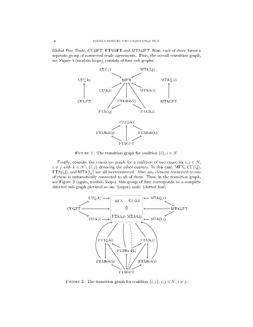
Global Free Trade, CUGFT, FTAGFT and MTAGFT. Now, each of those forms aseparate group of connected trade agreements. Thus, the overall transition graph,see Figure 1 (modulo loops), consists of four sub-graphs.
MFN
CU(i,j)
CU(k,i)
CU(j,k)
CUGFT
MTA(i,j)
MTA(k,i)
MTA(j,k)
MTAGFT
FTA(i,j) FTA(k,i)
FTAHub(i)
FTA(j,k)
FTAHub(j) FTAHub(k)
FTAGFT
Figure 1. The transition graph for coalition {i}, i ∈ N .
Finally, consider the transition graph for a coalition of two countries i, j ∈ N ,i 6= j with k ∈ N \ {i, j} denoting the other country. In this case, MFN, CU(i,j),FTA(i,j), and MTA(i,j) are all interconnected. Also, any element connected to oneof these is automatically connected to all of them. Thus, in the transition graph,see Figure 2 (again, modulo loops), this group of four corresponds to a completedirected sub-graph pictured as one `(super) node' (dotted box).
CU(i,j)
MTA(i,j)
MFN
FTA(i,j)
CU(j,k)
CU(k,i)
CUGFT
MTA(j,k)
MTA(k,i)
MTAGFT
FTA(j,k) FTA(k,i)
FTAHub(k)
FTAHub(j) FTAHub(i)
FTAGFT
Figure 2. The transition graph for coalition {i, j}, i, j ∈ N , i 6= j.
THE FARSIGHTED STABILITY OF GLOBAL TRADE POLICY ARRANGEMENTS 11
3.6. Algorithm and Parameters. The (additional) explanatory power from theintroduction of an extensive set of trade agreements and unlimited farsightednesscomes at the cost of a complex computational problem. This problem is solvednumerically with the help of an algorithm - the pseudocode of which can be found inAppendix A.19 The parameter space therefore needs to be speci�ed and discretized:
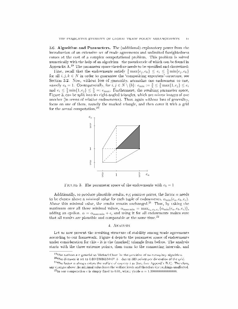
First, recall that the endowments satisfy 35 max{ej , ek} ≤ ei ≤ 5
3 min{ej , ek}for all i, j, k ∈ N in order to guarantee the `competiting exporters'-structure, seeSection 3.2. Now, without loss of generality, normalize one endowment to one,namely eb = 1. Consequentially, for i, j ∈ N \ {b}: emin := 3
5 ≤35 max{1, ej} ≤ ei
and ei ≤ 53 min{1, ej} ≤ 5
3 =: emax. Furthermore, the resulting parameter space,Figure 3, can be split into six right-angled triangles, which are mirror images of oneanother (in terms of relative endowments). Thus, again without loss of generality,focus on one of them, namely the marked triangle, and then cover it with a gridfor the actual computation.20
ec
ea35 1 5
3
35
1
53
Figure 3. The parameter space of the endowments with eb = 1
Additionally, to produce plausible results, e.g positive prices, the factor α needsto be chosen above a minimal value for each tuple of endowments, αmin(ea, eb, ec).Above this minimal value, the results remain unchanged.21 Thus, by taking themaximum over all these minimal values, αmaxmin = maxea,eb,ec{αmin(ea, eb, ec)},adding an epsilon, α = αmaxmin + ε, and using it for all endowments makes surethat all results are plausible and comparable at the same time.22
4. Analysis
Let us now present the resulting structure of stability among trade agreementsaccording to our framework. Figure 4 depicts the parameter space of endowmentsunder consideration for this - it is the (marked) triangle from before. The analysisstarts with the three extreme points, then turns to the connecting intervals, and
19The authors are grateful to Michael Chwe for the provision of an exemplary algorithm.20The distance is set to 0.0013360053440215 - due to 500 points per dimension of the grid.21The factor α always enters the welfare of country i as 2αei (see Appendix B.1). Therefore,
any changes above the minimal value leave the welfare levels and therefore the rankings una�ected.22In our computation ε is simply �xed to 0.01, which yields α = 1.3988888888888888.
12 STEFAN BERENS AND LASHA CHOCHUA
�nishes with the entire interior. In each of these cases, two scenarios are examined.The �rst scenario corresponds to the current WTO institutional arrangement whilethe second one assumes modi�ed WTO rules without Article XXIV Paragraph 5,which would prevent the formation of PTAs (speci�cally CUs and FTAs).
P Q
R
PQ
QRPR
A
ec
ea1 53
1
53
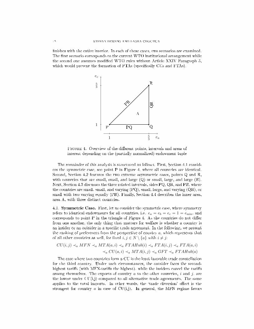
Figure 4. Overview of the di�erent points, intervals and areas ofinterest depending on the (partially normalized) endowment tuple
The remainder of this analysis is structured as follows. First, Section 4.1 consid-ers the symmetric case, see point P in Figure 4, where all countries are identical.Second, Section 4.2 features the two extreme asymmetric cases, points Q and R,with countries that are small, small, and large (Q) or small, large, and large (R).Next, Section 4.3 discusses the three related intervals, sides PQ, QR, and PR, wherethe countries are small, small, and varying (PQ), small, large, and varying (QR), orsmall with two varying equally (PR). Finally, Section 4.4 describes the inner area,area A, with three distinct countries.
4.1. Symmetric Case. First, let us consider the symmetric case, where symmetryrefers to identical endowments for all countries, i.e. ea = eb = ec = 1 = emin, andcorresponds to point P in the triangle of Figure 4. As the countries do not di�erfrom one another, the only thing that matters for welfare is whether a country isan insider or an outsider in a speci�c trade agreement. In the following, we presentthe ranking of preferences from the perspective of country a, which represents thatof all other countries as well, for �xed i, j ∈ N \ {a} with i 6= j:
CU(i, j) ≺a MFN ≺a MTA(a, i) ≺a FTAHub(i) ≺a FTA(i, j) ≺a FTA(a, i)
≺a CU(a, i) ≺a MTA(i, j) ≺a GFT ≺a FTAHub(a)
The case where two countries form a CU is the least favorable trade constellationfor the third country. Under such circumstances, the outsider faces the second-highest tari�s (with MFN-tari�s the highest), while the insiders cancel the tari�samong themselves. The exports of country a to the other countries, i and j, arethe lowest under CU(i,j) compared to all alternative trade agreements. The sameapplies to the total imports. In other words, the `trade diversion' e�ect is thestrongest for country a in case of CU(i,j). In general, the MFN regime favors
THE FARSIGHTED STABILITY OF GLOBAL TRADE POLICY ARRANGEMENTS 13
country a when compared to CU(i,j). The tari� revenue remains the same, whilethe consumer surplus is lower and the producer surplus is higher - the increaseo�sets the decrease. The MFN regime slackens the `trade diversion' e�ect presentin the case of CU(i,j) by virtue of increased export values of country a.
Among the group of bilateral trade agreements where the country is an insider,the MTAs result in the lowest welfare (for this country). MTA(a,i) itself generatesa higher welfare for country a in comparison with the MFN regime on the groundsof increased consumer and producer surplus. The FTAHub(i) constellation resultsin even further gains in welfare for country a through higher export values andproducer surplus accordingly (the tari� revenue and also the consumer surplus arelower under FTAHub(i) compared to MTA(a,i) though). However, country a doesnot have an incentive to remain in this constellation. The unilateral deviation fromFTAHub(i) to FTA(i,j) comes with a decrease of consumer and producer surplusbut enough increase in tari� revenue to ultimately ensure higher welfare under thelatter constellation. Nonetheless, among FTAs being an outsider is less desirablethan being an insider for any country. The drop in tari� revenue is o�set by anexpansion of the consumer and producer surplus, resulting in higher welfare forcountry a in case of FTA(a,i) compared to FTA(i,j). As an insider, country aprefers CU(a,i) over FTA(a,i) though. More precisely, in spite of the decline in theconsumer surplus, the actual welfare goes up through an expansion of tari� revenueand producer surplus.
The formation of MTA(i,j) guarantees the highest welfare for country a comparedto any other bilateral trade agreement. The driving factor is the MFN-principle,which implies that in case of MTA(i,j) the insiders need to apply the same tari� toboth each other and the outsider - a form of free-rider problem. At the same time,country a attains the highest possible tari� revenue.
Each country obtains the second-highest welfare level when the world reachesglobal free trade. Under full trade liberalization, the producer surplus is also thesecond-highest among all trade agreements (e�ectively driving the ranking). Itis only surpassed by that of FTAHub(a). The latter constellation brings aboutthe highest possible welfare for country a. But note that such a trade agreementdisproportionally favors the hub country over the other countries.
Countries' strong preference rankings are the crucial ingredient for computingthe LCS. In fact, for each country all three variants of global free trade are rankedas second-best option while each �rst-best option, a hub structure, is ranked con-siderably lower for the other countries. Intuitively, global free trade seems like astable compromise. The following proposition and its proof reinforce this:
Proposition 3. Under symmetry and with the current institutional arrangementof the WTO, the LCS contains three elements: CUGFT, FTAGFT, and MTAGFT.In other words, (the trinity of) global free trade is the unique stable outcome.
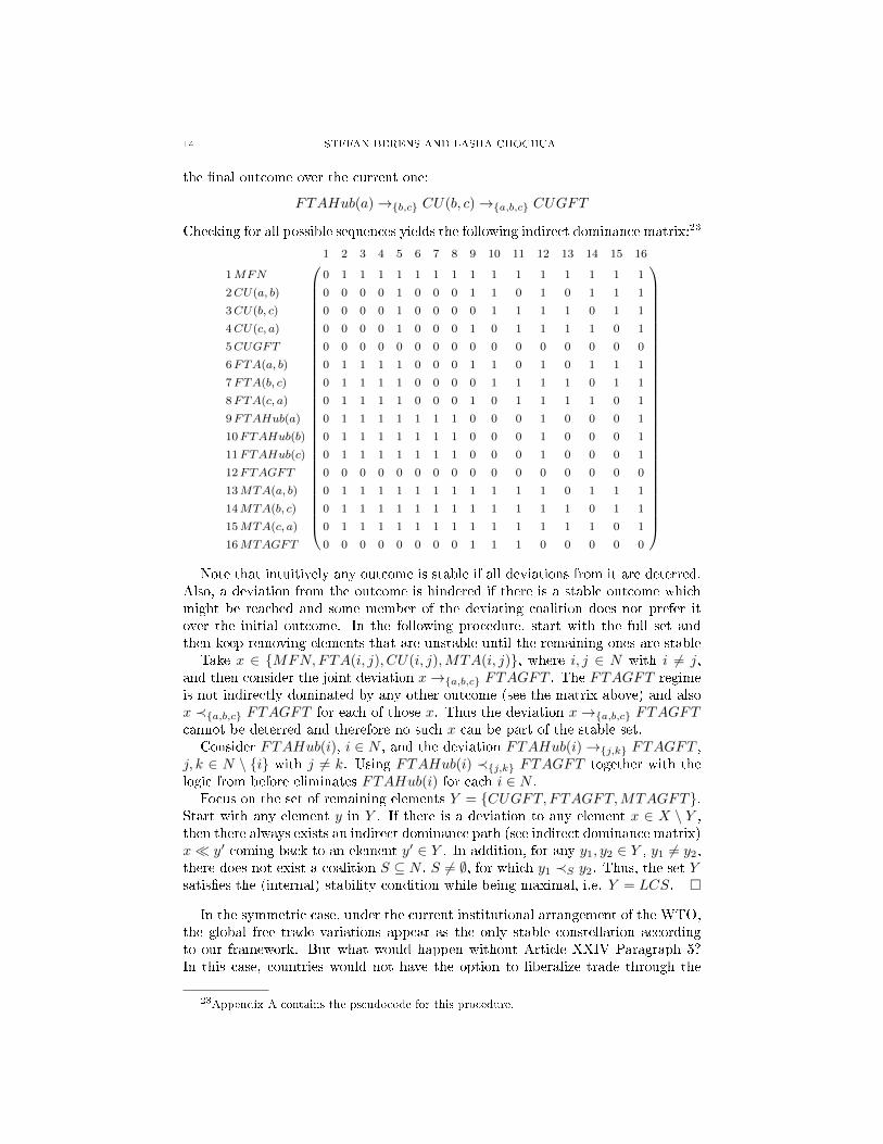
Proof. Based on the de�nition of indirect dominance and the transition graphs,see Section 3.4 and 3.5, the preference rankings from earlier allow us to derive theindirect dominance matrix. If the entry in the matrix is equal to one (resp. zero),then the trade arrangement corresponding to the row of the entry is (resp. isn't)indirectly dominated by the one corresponding to the column of the entry. Forexample, FTAHub(a) is indirectly dominated by CUGFT as there exists a (�nite)sequence of outcomes and coalitions such that all coalitions in the sequence prefer
14 STEFAN BERENS AND LASHA CHOCHUA
the �nal outcome over the current one:
FTAHub(a)→{b,c} CU(b, c)→{a,b,c} CUGFT
Checking for all possible sequences yields the following indirect dominance matrix:23
1 2 3 4 5 6 7 8 9 10 11 12 13 14 15 16
1MFN 0 1 1 1 1 1 1 1 1 1 1 1 1 1 1 1
2CU(a, b) 0 0 0 0 1 0 0 0 1 1 0 1 0 1 1 1
3CU(b, c) 0 0 0 0 1 0 0 0 0 1 1 1 1 0 1 1
4CU(c, a) 0 0 0 0 1 0 0 0 1 0 1 1 1 1 0 1
5CUGFT 0 0 0 0 0 0 0 0 0 0 0 0 0 0 0 0
6FTA(a, b) 0 1 1 1 1 0 0 0 1 1 0 1 0 1 1 1
7FTA(b, c) 0 1 1 1 1 0 0 0 0 1 1 1 1 0 1 1
8FTA(c, a) 0 1 1 1 1 0 0 0 1 0 1 1 1 1 0 1
9FTAHub(a) 0 1 1 1 1 1 1 1 0 0 0 1 0 0 0 1
10FTAHub(b) 0 1 1 1 1 1 1 1 0 0 0 1 0 0 0 1
11FTAHub(c) 0 1 1 1 1 1 1 1 0 0 0 1 0 0 0 1
12FTAGFT 0 0 0 0 0 0 0 0 0 0 0 0 0 0 0 0
13MTA(a, b) 0 1 1 1 1 1 1 1 1 1 1 1 0 1 1 1
14MTA(b, c) 0 1 1 1 1 1 1 1 1 1 1 1 1 0 1 1
15MTA(c, a) 0 1 1 1 1 1 1 1 1 1 1 1 1 1 0 1
16MTAGFT 0 0 0 0 0 0 0 0 1 1 1 0 0 0 0 0
Note that intuitively any outcome is stable if all deviations from it are deterred.
Also, a deviation from the outcome is hindered if there is a stable outcome whichmight be reached and some member of the deviating coalition does not prefer itover the initial outcome. In the following procedure, start with the full set andthen keep removing elements that are unstable until the remaining ones are stable
Take x ∈ {MFN,FTA(i, j), CU(i, j),MTA(i, j)}, where i, j ∈ N with i 6= j,and then consider the joint deviation x→{a,b,c} FTAGFT . The FTAGFT regimeis not indirectly dominated by any other outcome (see the matrix above) and alsox ≺{a,b,c} FTAGFT for each of those x. Thus the deviation x→{a,b,c} FTAGFTcannot be deterred and therefore no such x can be part of the stable set.
Consider FTAHub(i), i ∈ N , and the deviation FTAHub(i)→{j,k} FTAGFT ,j, k ∈ N \ {i} with j 6= k. Using FTAHub(i) ≺{j,k} FTAGFT together with thelogic from before eliminates FTAHub(i) for each i ∈ N .
Focus on the set of remaining elements Y = {CUGFT, FTAGFT,MTAGFT}.Start with any element y in Y . If there is a deviation to any element x ∈ X \ Y ,then there always exists an indirect dominance path (see indirect dominance matrix)x� y′ coming back to an element y′ ∈ Y . In addition, for any y1, y2 ∈ Y , y1 6= y2,there does not exist a coalition S ⊆ N , S 6= ∅, for which y1 ≺S y2. Thus, the set Ysatis�es the (internal) stability condition while being maximal, i.e. Y = LCS. �
In the symmetric case, under the current institutional arrangement of the WTO,the global free trade variations appear as the only stable constellation accordingto our framework. But what would happen without Article XXIV Paragraph 5?In this case, countries would not have the option to liberalize trade through the
23Appendix A contains the pseudocode for this procedure.
THE FARSIGHTED STABILITY OF GLOBAL TRADE POLICY ARRANGEMENTS 15
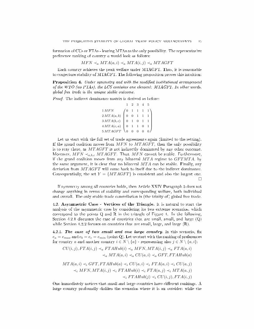
formation of CUs or FTAs - leaving MTAs as the only possibility. The representativepreference ranking of country a would look as follows:
MFN ≺a MTA(a, i) ≺a MTA(i, j) ≺a MTAGFT
Each country achieves the peak welfare under MTAGFT. Thus, it is reasonableto conjecture stability of MTAGFT. The following proposition proves this intuition:
Proposition 4. Under symmetry and with the modi�ed institutional arrangementof the WTO (no PTAs), the LCS contains one element: MTAGFT. In other words,global free trade is the unique stable outcome.
Proof. The indirect dominance matrix is derived as before:
1 2 3 4 5
1MFN 0 1 1 1 1
2MTA(a, b) 0 0 1 1 1
3MTA(b, c) 0 1 0 1 1
4MTA(c, a) 0 1 1 0 1
5MTAGFT 0 0 0 0 0
Let us start with the full set of trade agreements again (limited to the setting).
If the grand coalition moves from MFN to MTAGFT , then the only possibilityis to stay there, as MTAGFT is not indirectly dominated by any other outcome.Moreover, MFN ≺a,b,c MTAGFT . Thus, MFN cannot be stable. Furthermore,if the grand coalition moves from any bilateral MTA regime to GFTMTA, bythe same argument, it is clear that no bilateral MTA can be stable. Finally, anydeviation from MTAGFT will come back to itself due to the indirect dominance.Consequentially, the set Y = {MTAGFT} is consistent and also the largest one.
�
If symmetry among all countries holds, then Article XXIV Paragraph 5 does notchange anything in terms of stability and corresponding welfare, both individualand overall. The only stable trade constellation is (the trinity of) global free trade.
4.2. Asymmetric Case - Vertices of the Triangle. It is natural to start theanalysis of the asymmetric case by considering its two extreme scenarios, whichcorrespond to the points Q and R in the triangle of Figure 4. In the following,Section 4.2.1 discusses the case of countries that are small, small, and large (Q)while Section 4.2.2 focuses on countries that are small, large, and large (R).
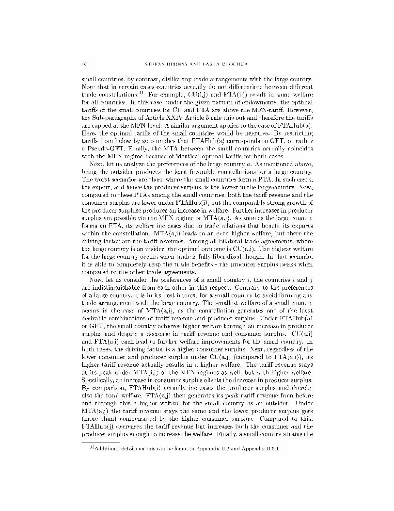
4.2.1. The case of two small and one large country. In this scenario, �xea = emax and eb = ec = emin (point Q). Let us start with the ranking of preferencesfor country a and another country i ∈ N \ {a} - representing also j ∈ N \ {a, i}:
CU(i, j), FTA(i, j) ≺a FTAHub(i) ≺a MFN,MTA(i, j) ≺a FTA(a, i)
≺a MTA(a, i) ≺a CU(a, i) ≺a GFT, FTAHub(a)
MTA(a, i) ≺i GFT, FTAHub(a) ≺i CU(a, i) ≺i FTA(a, i) ≺i CU(a, j)
≺i MFN,MTA(i, j) ≺i FTAHub(i) ≺i FTA(a, j) ≺i MTA(a, j)
≺i FTAHub(j) ≺i CU(i, j), FTA(i, j)
One immediately notices that small and large countries have di�erent rankings. Alarge country profoundly dislikes the scenarios where it is an outsider; while the
16 STEFAN BERENS AND LASHA CHOCHUA
small countries, by contrast, dislike any trade arrangements with the large country.Note that in certain cases countries actually do not di�erentiate between di�erenttrade constellations.24 For example, CU(i,j) and FTA(i,j) result in same welfarefor all countries. In this case, under the given pattern of endowments, the optimaltari�s of the small countries for CU and FTA are above the MFN-tari�. However,the Sub-paragraphs of Article XXIV Article 5 rule this out and therefore the tari�sare capped at the MFN-level. A similar argument applies to the case of FTAHub(a).Here, the optimal tari�s of the small countries would be negative. By restrictingtari�s from below by zero implies that FTAHub(a) corresponds to GFT, or rathera Pseudo-GFT. Finally, the MTA between the small countries actually coincideswith the MFN regime because of identical optimal tari�s for both cases.
Next, let us analyze the preferences of the large country a. As mentioned above,being the outsider produces the least favorable constellations for a large country.The worst scenarios are those where the small countries form a PTA. In such cases,the export, and hence the producer surplus, is the lowest in the large country. Now,compared to these PTAs among the small countries, both the tari� revenue and theconsumer surplus are lower under FTAHub(i), but the comparably strong growth ofthe producer surpluse produces an increase in welfare. Further increases in producersurplus are possible via the MFN regime or MTA(a,i). As soon as the large countryforms an FTA, its welfare increases due to trade relations that bene�t its exportswithin the constellation. MTA(a,i) leads to an even higher welfare, but there thedriving factor are the tari� revenues. Among all bilateral trade agreements, wherethe large country is an insider, the optimal outcome is CU(a,i). The highest welfarefor the large country occurs when trade is fully liberalized though. In that scenario,it is able to completely reap the trade bene�ts - the producer surplus peaks whencompared to the other trade agreements.
Now, let us consider the preferences of a small country i, the countries i and jare indistinguishable from each other in this respect. Contrary to the preferencesof a large country, it is in its best interest for a small country to avoid forming anytrade arrangement with the large country. The smallest welfare of a small countryoccurs in the case of MTA(a,i), as the constellation generates one of the leastdesirable combinations of tari� revenue and producer surplus. Under FTAHub(a)or GFT, the small country achieves higher welfare through an increase in producersurplus and despite a decrease in tari� revenue and consumer surplus. CU(a,i)and FTA(a,i) each lead to further welfare improvements for the small country. Inboth cases, the driving factor is a higher consumer surplus. Next, regardless of thelower consumer and producer surplus under CU(a,j) (compared to FTA(a,i)), itshigher tari� revenue actually results in a higher welfare. The tari� revenue staysat its peak under MTA(i,j) or the MFN regimes as well, but with higher welfare.Speci�cally, an increase in consumer surplus o�sets the decrease in producer surplus.By comparison, FTAHub(i) actually increases the producer surplus and therebyalso the total welfare. FTA(a,j) then generates its peak tari� revenue from beforeand through this a higher welfare for the small country as an outsider. UnderMTA(a,j) the tari� revenue stays the same and the lower producer surplus gets(more than) compensated by the higher consumer surplus. Compared to this,FTAHub(j) decreases the tari� revenue but increases both the consumer and theproducer surplus enough to increase the welfare. Finally, a small country attains the
24Additional details on this can be found in Appendix B.2 and Appendix B.5.1.
THE FARSIGHTED STABILITY OF GLOBAL TRADE POLICY ARRANGEMENTS 17
best result by forming a PTA with the other small country, either through FTA(i,j)or CU(i,j). While keeping relatively high tari� revenues, the small countries manageto have a high producer surplus as well.
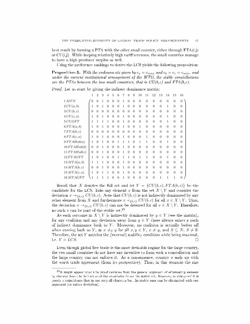
Using the preference rankings to derive the LCS yields the following proposition:
Proposition 5. With the endowments given by ea = emax and eb = ec = emin, andunder the current institutional arrangement of the WTO, the stable constellationsare the PTAs between the two small countries, that is CU(b,c) and FTA(b,c).
Proof. Let us start by giving the indirect dominance matrix:
1 2 3 4 5 6 7 8 9 10 11 12 13 14 15 16
1MFN 0 0 1 0 0 0 1 0 0 0 0 0 0 0 0 0
2CU(a, b) 1 0 1 0 0 0 1 0 0 0 0 0 0 1 0 0
3CU(b, c) 0 0 0 0 0 0 0 0 0 0 0 0 0 0 0 0
4CU(c, a) 1 0 1 0 0 0 1 0 0 0 0 0 0 1 0 0
5CUGFT 1 1 1 1 0 0 1 0 0 0 0 0 0 1 0 0
6FTA(a, b) 1 0 1 0 0 0 1 0 0 1 0 0 0 0 0 0
7FTA(b, c) 0 0 0 0 0 0 0 0 0 0 0 0 0 0 0 0
8FTA(c, a) 1 0 1 0 0 0 1 0 0 0 1 0 0 0 0 0
9FTAHub(a) 1 0 1 0 0 1 1 1 0 1 1 0 0 1 0 0
10FTAHub(b) 0 0 1 0 0 0 1 0 0 0 0 0 0 0 0 0
11FTAHub(c) 0 0 1 0 0 0 1 0 0 0 0 0 0 0 0 0
12FTAGFT 1 0 1 0 0 1 1 1 0 1 1 0 0 1 0 0
13MTA(a, b) 1 1 1 0 0 0 1 0 0 0 0 0 0 0 0 0
14MTA(b, c) 0 0 1 0 0 0 1 0 0 0 0 0 0 0 0 0
15MTA(c, a) 1 0 1 1 0 0 1 0 0 0 0 0 0 0 0 0
16MTAGFT 1 1 1 1 0 0 1 0 0 0 0 0 1 1 1 0
Recall that X denotes the full set and let Y = {CU(b, c), FTA(b, c)} be the
candidate for the LCS. Take any element x from the set X \ Y and consider thedeviation x→{b,c} CU(b, c). Note that CU(b, c) is not indirectly dominated by anyother element from X and furthermore x ≺{b,c} CU(b, c) for all x ∈ X \ Y . Thus,the deviation x →{b,c} CU(b, c) can not be deterred for all x ∈ X \ Y . Therefore,no such x can be part of the stable set.25
As each outcome in X \ Y is indirectly dominated by y ∈ Y (see the matrix),for any coalition and any deviation away from y ∈ Y there always exists a pathof indirect dominance back to Y . Moreover, no coalition is actually better o�when coming back to Y , as x 6≺S y for all x, y ∈ Y , x 6= y, and S ⊆ N , S 6= ∅.Therefore, the set Y satis�es the (internal) stability condition while being maximal,i.e. Y = LCS. �
Even though global free trade is the most desirable regime for the large country,the two small countries do not have any incentive to form such a constellation andthe large country can not enforce it. As a consequence, country a ends up withthe worst trade agreement (from its perspective). Thus, in this scenario the size
25It might appear that this proof deviates from the general approach of eliminating elementby element from the full set until the remainder forms the stable set. However, in this proof it ispurely a coincidence that in one step all elements but the stable ones can be eliminated with oneargument (or rather deviation).
18 STEFAN BERENS AND LASHA CHOCHUA
advantage of the large country does not translate into a favorable stable regime.Moreover, this speci�c case showcases the relevance of the restrictions on PTAs(remember that insiders are not allowed to raise tari�s on outsiders). The constraintmakes the small countries be indi�erent between the two forms of PTAs.
Now we turn to the hypothetical scenario without Article XXIV Paragraph 5.Here, the ranking of preferences for the countries, with country a the large one andcountry b and c small (represented by i and j), are as follows:
MTA(i, j),MFN ≺a MTA(a, i) ≺a GFT
MTA(a, i) ≺i MTAGFT ≺i MFN,MTA(i, j) ≺i MTA(a, j)
As a result, the best outcome for a small country i is the MTA(i, j) regime, as thePTAs are not available anymore. The next proposition presents the new LCS as aconsequence of these changes:
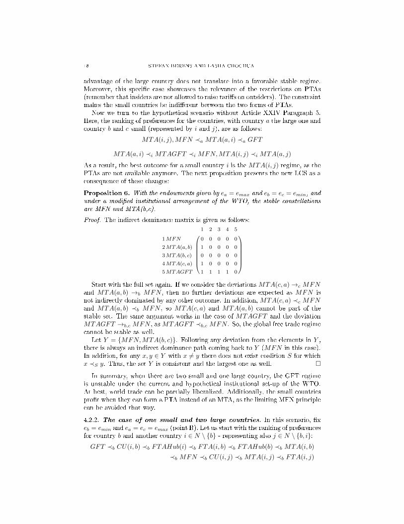
Proposition 6. With the endowments given by ea = emax and eb = ec = emin, andunder a modi�ed institutional arrangement of the WTO, the stable constellationsare MFN and MTA(b,c).
Proof. The indirect dominance matrix is given as follows:
1 2 3 4 5
1MFN 0 0 0 0 0
2MTA(a, b) 1 0 0 0 0
3MTA(b, c) 0 0 0 0 0
4MTA(c, a) 1 0 0 0 0
5MTAGFT 1 1 1 1 0
Start with the full set again. If we consider the deviations MTA(c, a)→c MFN
and MTA(a, b) →b MFN , then no further deviations are expected as MFN isnot indirectly dominated by any other outcome. In addition, MTA(c, a) ≺c MFNand MTA(a, b) ≺b MFN , so MTA(c, a) and MTA(a, b) cannot be part of thestable set. The same argument works in the case of MTAGFT and the deviationMTAGFT →b,c MFN , asMTAGFT ≺b,c MFN . So, the global free trade regimecannot be stable as well.
Let Y = {MFN,MTA(b, c)}. Following any deviation from the elements in Y ,there is always an indirect dominance path coming back to Y (MFN in this case).In addition, for any x, y ∈ Y with x 6= y there does not exist coalition S for whichx ≺S y. Thus, the set Y is consistent and the largest one as well. �
In summary, when there are two small and one large country, the GFT regimeis unstable under the current and hypothetical institutional set-up of the WTO.At best, world trade can be partially liberalized. Additionally, the small countriespro�t when they can form a PTA instead of an MTA, as the limiting MFN principlecan be avoided that way.
4.2.2. The case of one small and two large countries. In this scenario, �xeb = emin and ea = ec = emax (point R). Let us start with the ranking of preferencesfor country b and another country i ∈ N \ {b} - representing also j ∈ N \ {b, i}:GFT ≺b CU(i, b) ≺b FTAHub(i) ≺b FTA(i, b) ≺b FTAHub(b) ≺b MTA(i, b)
≺b MFN ≺b CU(i, j) ≺b MTA(i, j) ≺b FTA(i, j)

THE FARSIGHTED STABILITY OF GLOBAL TRADE POLICY ARRANGEMENTS 19
CU(j, b) ≺i FTA(j, b) ≺i MFN ≺i MTA(i, b),MTA(j, b) ≺i FTA(i, j)
≺i MTA(i, j) ≺i CU(i, j) ≺i FTAHub(b) ≺i FTAHub(j) ≺i GFT
≺i FTAHub(i) ≺i FTA(i, b) ≺i CU(i, b)
Under the given pattern of endowments, the preference rankings of the countriesare considerably di�erent from the previous cases. For the small country, the MFNregime generates higher welfare than any other trade agreement where it is part of.As for a large country, being an outsider is on the lower end of the ranking, whilebeing an insider in a PTA with a small country is on the other end.
Let us take a closer look at the preference ranking of the small country. First,GFT actually generates the lowest total welfare - driven by no tari� revenue and notenough compensation via consumer and producer surplus. As mentioned before,any trade arrangement involving the small country results in lower welfare comparedwith other constellations (but higher welfare than GFT). The lowest among thoseare the CU with any of the large countries, which through increased tari� revenue(and despite a decrease in consumer surplus) yield higher welfare in comparison withthe GFT regime. Even though FTAHub(i) reduces those gains in tari� revenueagain, by virtue of a growing consumer surplus it still raises the total welfare.Further improvement in the welfare of the small country is possible if the worldmoves from FTAHub(i) to FTA(i,b); the sole reason is a higher consumer surplus.Under FTAHub(b), the export volumes to the large countries are at its peak and itgenerates substantially higher producer surplus. As a consequence, it results in thesmall country preferring to form a hub structure (as the hub node) over an FTA withone of the large countries. Replacing the FTA with an MTA with similar structureis the most desirable con�guration for the small country among the constellationswhere it participates. Under MTA(i,b) the producer surplus is actually the smallestcompared to all other alternatives, but high tari� revenue and consumer surplusdetermine its position in the ranking. The MFN regime surpasses all con�gurationsmentioned above. When there are two large countries, the tari� revenue becomesan important factor in the welfare of the small country. Any further improvementswith respect to the welfare of the small country depend on the large countriesliberalizing trade among themselves - the small country essentially free-rides inthese cases (exhausting its tari� revenue to the fullest). The driving factor amongthese three is the export volume. Consequentially, CU(i,j) is the worst option,followed by MTA(i,j), and FTA(i,j) is the (overall) best outcome.
The following discusses the preferences of the two large countries. The leastfavorable scenario occurs when the other large country forms a CU together withthe small country. Its position in the ranking is driven by the lowest export volumesand producer surplus. Now, FTA(j,b) produces higher welfare compared to theprevious constellation due to growth in producer surplus (based on rising exportsto the small country) which makes up for the drop in consumer surplus. A similardevelopment makes the MFN regime an even better constellation (here the exportsto the large country increase). All tari�s (and thus prices) are identical underboth MTA(i,b) and MTA(j,b), as a consequence they generate the same welfare.On the grounds of increased exports, the welfare tops that of the MFN regime.Among the class of bilateral trade agreements between the large countries, theranking goes as follows: FTA(i,j) followed by MTA(i,j) only surpassed by CU(i,j).In comparison with MTA(i,b) and MTA(j,b), the greater consumer and producer
20 STEFAN BERENS AND LASHA CHOCHUA
surplus of FTA(i,j) guarantees an increase of total welfare. An MTA between thetwo large countries produces more tari� revenues and actually results in a moredesirable outcome. Moving from MTA(i,j) to CU(i,j) decreases tari� revenue andalso consumer surplus but the gain in producer surplus through increased exportsto the other large country makes more than up for this. FTAHub(b) and evenmore so FTAHUb(j) further improve the welfare via growth of the tari� revenueand consumer surplus (the case of FTAHub(b)), and increased exports to the otherlarge country (for FTAHUb(j)). Now, the GFT regime allows the large country toraise the exports to the small country while retaining the same level of exports tothe other large country. As a consequence, the welfare of GFT surpasses that of theprevious mentioned constellations. However, when the large country is part of a hubstructure as the hub node itself, then its exports to the small country increase suchthat the welfare exceeds that of full trade liberalization. Furthermore, the FTAwith the small country constitutes the second-best outcome for the large countryon the grounds of high tari� revenue accompanied by similar consumer surplus.Finally, CU(i,b) is the most desirable constellation driven by the high exports tothe small country.
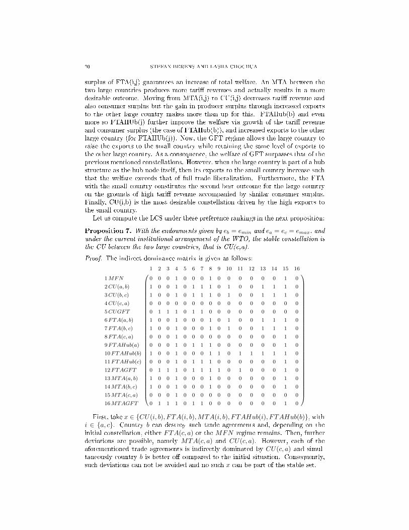
Let us compute the LCS under these preference rankings in the next proposition:
Proposition 7. With the endowments given by eb = emin and ea = ec = emax, andunder the current institutional arrangement of the WTO, the stable constellation isthe CU between the two large countries, that is CU(c,a).
Proof. The indirect dominance matrix is given as follows:
1 2 3 4 5 6 7 8 9 10 11 12 13 14 15 16
1MFN 0 0 0 1 0 0 0 1 0 0 0 0 0 0 1 0
2CU(a, b) 1 0 0 1 0 1 1 1 0 1 0 0 1 1 1 0
3CU(b, c) 1 0 0 1 0 1 1 1 0 1 0 0 1 1 1 0
4CU(c, a) 0 0 0 0 0 0 0 0 0 0 0 0 0 0 0 0
5CUGFT 0 1 1 1 0 1 1 0 0 0 0 0 0 0 0 0
6FTA(a, b) 1 0 0 1 0 0 0 1 0 1 0 0 1 1 1 0
7FTA(b, c) 1 0 0 1 0 0 0 1 0 1 0 0 1 1 1 0
8FTA(c, a) 0 0 0 1 0 0 0 0 0 0 0 0 0 0 1 0
9FTAHub(a) 0 0 0 1 0 1 1 1 0 0 0 0 0 0 1 0
10FTAHub(b) 1 0 0 1 0 0 0 1 1 0 1 1 1 1 1 0
11FTAHub(c) 0 0 0 1 0 1 1 1 0 0 0 0 0 0 1 0
12FTAGFT 0 1 1 1 0 1 1 1 1 0 1 0 0 0 1 0
13MTA(a, b) 1 0 0 1 0 0 0 1 0 0 0 0 0 0 1 0
14MTA(b, c) 1 0 0 1 0 0 0 1 0 0 0 0 0 0 1 0
15MTA(c, a) 0 0 0 1 0 0 0 0 0 0 0 0 0 0 0 0
16MTAGFT 0 1 1 1 0 1 1 0 0 0 0 0 0 0 1 0
First, take x ∈ {CU(i, b), FTA(i, b),MTA(i, b), FTAHub(i), FTAHub(b)}, with
i ∈ {a, c}. Country b can destroy such trade agreements and, depending on theinitial constellation, either FTA(c, a) or the MFN regime remains. Then, furtherdeviations are possible, namely MTA(c, a) and CU(c, a). However, each of theaforementioned trade agreements is indirectly dominated by CU(c, a) and simul-taneously country b is better o� compared to the initial situation. Consequently,such deviations can not be avoided and no such x can be part of the stable set.

THE FARSIGHTED STABILITY OF GLOBAL TRADE POLICY ARRANGEMENTS 21
Now, consider x ∈ {MFN,FTA(c, a),MTA(c, a)} for which x →{a,c} CU(a, c)presents a deviation that can not be deterred. As in the previous paragraph,CU(c, a) is not indirectly dominated any element and also x ≺{a,c} CU(a, c). Thus,no such x can be the part of the stable set as well.
At last, let x ∈ {CUGFT, FTAGFT,MTAGFT} and consider the deviationswhere country b leaves the agreements. CU(c, a), FTA(c, a), or MTA(c, a) canbe the result. We have shown that the last two outcomes can not be stable. Asfor CU(a, c), we have that for all x considered x ≺{b} CU(a, c). As a result, weconclude that no such x can be in the consistent set.CU(a, c) indirectly dominates each outcome, all deviations from it are deterred.
So, the set containing CU(a, c) is consistent and the largest one as well. �
The small country manages to block many desirable outcomes for large countries.Country b can unilaterally deviate from any trade agreement with higher welfarethan CU(i,j) for the large countries. Thus, the majority of countries cannot imposetheir will on the other country. What the large countries can achieve is the besttrade agreement that they can reach without the participation of the small country,in this case one among themselves.
A similar story unfolds in the scenario without Article XXIV Paragraph 5. There,the countries' preference rankings are as follows, with country b the small one andcountry a and c large (represented by i and j):
MTAGFT ≺b MTA(i, b) ≺b MFN ≺b MTA(i, j)
MFN ≺i MTA(i, b),MTA(j, b) ≺i MTA(i, j) ≺i MTAGFT
As the logic of the corresponding preference rankings of the countries is similarto before, let us directly present the proposition:
Proposition 8. With the endowments given by eb = emin and ea = ec = emax, andunder a modi�ed institutional arrangement of the WTO, the stable constellation isthe MTA between the two large countries, that is MTA(c,a).
Proof. In this case, the indirect dominance matrix has the following form:
1 2 3 4 5
1MFN 0 0 0 1 0
2MTA(a, b) 1 0 0 1 0
3MTA(b, c) 1 0 0 1 0
4MTA(c, a) 0 0 0 0 0
5MTAGFT 0 0 0 1 0
Assume, x ∈ {MTA(a, b),MTA(b, c),MTAGFT} and consider the deviations,
where country b dismantles any above mentioned constellation. Two possibilities:Either MFN or MTA(c, a) remain. From MFN either no coalition moves awayor, as it is indirectly dominated byMTA(c, a) (see the indirect dominance matrix),the latter might be approached. In either case, b is better o�. Thus, no such x canbe part of the stable set.
Now, analyze the case of the MFN regime. Take the following deviation:MFN →{a,c} MTA(c, a). As MTA(c, a) is not indirectly dominated by any othertrade agreement and MFN ≺{a,c} MTA(c, a), the MFN regime can not be stableas well.
22 STEFAN BERENS AND LASHA CHOCHUA
As MTA(c, a) indirectly dominates each trade agreement, all deviations from itare deterred. So, the set consisting of MTA(c, a) is consistent and the largest oneas well. �
Thus, similar to the other asymmetric case, one small and two large countriesallow for partial but not full liberalization of world trade irrespective of the actualscenario (current vs. modi�ed WTO rules). In terms of overall welfare, the world isbetter o� in the hypothetical scenario without Article XXIV Paragraph 5 though.Individually, the small country is in a better position in case of MTA(i,j) comparedto CU(i,j), as it exploits the MFN obligation of the large countries. By contrast,the large countries are better o� in the other case. Therefore, while none of the twoinstitutional arrangement facilitate global free trade, they in�uence the welfare forthe stable set (both overall and individual).
4.3. Asymmetric Case - Edges of the Triangle. Let us now turn to the caseswhere the endowments of countries vary along one dimension - corresponding to thesides PQ, QR, and PR in the triangle of Figure 4. Speci�cally, Section 4.3.1 presentsthe scenario where the countries are small, small, and varying (PQ), Section 4.3.2discusses the setting where the countries are small, large, and varying (QR), andSection 4.3.3 describes the case of a small country with two varying equally (PR).
While in the previous cases it was still possible to solve the problems analytically,the following require the use of a numerical approach. The analysis presented hereconsists of graphics picturing the composition of the stable sets and accompanyingdescriptions that explore the underlying mechanics. The exact numerical values forthese (sub-)intervals can be found in Section C.2.
4.3.1. The case of one small, one large, and one varying country. First,let us consider the case eb = emin, ea = emax, and ec ∈ (emin, emax) (side QR).Under the given pattern of the endowments, a number of trade agreements can becompletely ruled out (with respect to the LCS). The MFN and GFT regimes forexample are never part of the stable set. Additionally, none of the PTAs betweenthe small and the large country appear as a stable outcome. The same holds forthe hub structures where either the small or the large country is the hub node. Asfor the actual composition of the LCS, see Figure 5 for a graphical representation.
The general observation is that when the varying country is close in size to thesmall country, then the PTAs between these smaller countries appear as elementsin the stable set. When the country becomes larger the trade constellation betweenthe larger countries replaces these. Additionally, there are two small, separated,regions in the middle of the interval where FTAHub(c) is stable.
In order to get an intuitive understanding of the results, let us identify speci�ctrade agreements that go from stable to unstable (or the other way around) forcertain endowment tuples. Then, explore the underlying mechanics to understandwhy the changes happen.
Start with the PTAs between country b and c, the small and the varying one.Interestingly, the only factor driving their stability are the preferences of country b(with �xed minimal endowments). Once the MFN regime becomes more desirablethan CU(b,c) for country b, the constellation CU(b,c) drops from the stable set.Now, an identical story holds for the case of FTA(b,c). Thus, for both constellationsit only requires a single change in the preference ranking of country b to in�uencethe stable set.

THE FARSIGHTED STABILITY OF GLOBAL TRADE POLICY ARRANGEMENTS 23
CU(b,c)
CU(c,a)
FTA(b,c)
FTA(c,a)
FTAHub(c)
MTA(c,a)
1= eb
53
= ea
ec
Figure 5. Characterization of the case of small, varying, and largecountry
The PTAs and MTAs between country a and c start to appear in the LCS whencountry c is becoming relatively large and closer to country a in size. At �rst bothcountries actually prefer to form a CU with country b, that is when country c isrelatively small (and CU(b,c) actually is an element in the stable set). However,once it is preferable for country b to be the outsider instead of the insider in a CU,CU(c,a) emerges as a stable outcome (even though CU(b,c) still remains stable).Moreover, as soon as country c prefers FTA(c,a) respectively MTA(c,a) over theMFN regime, each of them becomes part of the LCS as well. For the interval whereall PTAs and MTAs between country a and c are stable, both countries have �xedpreference relations over these outcomes:
FTA(c, a) ≺a CU(c, a) ≺a MTA(c, a)
MTA(c, a) ≺c FTA(c, a) ≺c CU(c, a)
However, as soon as country c also prefers MTA(c,a) over FTA(c,a), the joint FTAdrops out of the LCS. Similarly, as soon as country a prefers CU(c,a) over MTA(c,a),this also applies to the joint MTA - leaving CU(c,a) as the only stable outcome.
FTAHub(c) is stable in the two small, separated, regions in (or near) the middleof the interval. In the �rst region, the stability is driven by the fact that country bstarts to value FTAHub(c) more than FTA(b,c) and gets in unison with country ain this respect. Once the preferences of country b over these outcomes get reversed,FTAHub(c) drops out of LCS again. In the second region, the stability of the samehub structure is largely determined by the change in the preferences of country c.Now, as soon as it starts to value FTA(c,a) over the MFN regime, which also putsFTA(c,a) in the LCS, both FTAs with c as a partner are stable and consequentiallythe corresponding hub structure is stable as well. As soon as the free-riding incen-tives of country b increase (valuing the MFN regime more than FTAHub(c)), thishub structure is not part of the stable set anymore.
The hypothetical institutional arrangement without Article XXIV Paragraph 5does not promote the appearance of GFT as part of the stable set. GFTMTA, butalso MTA(a,b) and MTA(b,c) never emerge as stable outcomes. Varying the size

24 STEFAN BERENS AND LASHA CHOCHUA
of country c generates either the MFN regime or MTA(c,a) as the stable element.Figure 6 presents these �ndings.26
MFN
MTA(b,c)
MTA(c,a)
1= eb
53
= ea
ec
Figure 6. Characterization of the case of small, varying, and largecountry
Over the whole interval, country b does not have any incentive to form an MTAwith any of the other countries. This is one reason why the MFN regime is stableover the speci�c range of the interval. The other reason is that country c prefers tonot have a trade agreement with country a as long as its own size is not too large.Once country c gets su�ciently large though, MTA(c,a) presents a better optionthan the MFN regime. As a consequence, MTA(c,a) replaces the MFN regime asthe stable set.
As a sidenote, while in the �rst scenario (with PTAs), the LCS near and at eachrespective extreme point corresponded to each other (continuity), the situation isdi�erent in the second scenario (without PTAs). When country c and b are equalin size, MTA(b,c) appears in the LCS even though it is not there before. Here,both the MFN regime and MTA(b,c) generate the same welfares for all countries(see also the discussion on point Q in Section 4.2.1).
Finally, under this given pattern of endowments, the GFT regime does not appearas part of the stable set independent of the scenario (with and without PTAs).However, the choice of rules does determine whether partial trade liberalizationtakes place or not. The possibility of forming PTAs reduces the incentive of thesmall(est) country to free ride. Otherwise, the MFN regime is the unique stableoutcome when there is one small, one large, and one comparably small country.
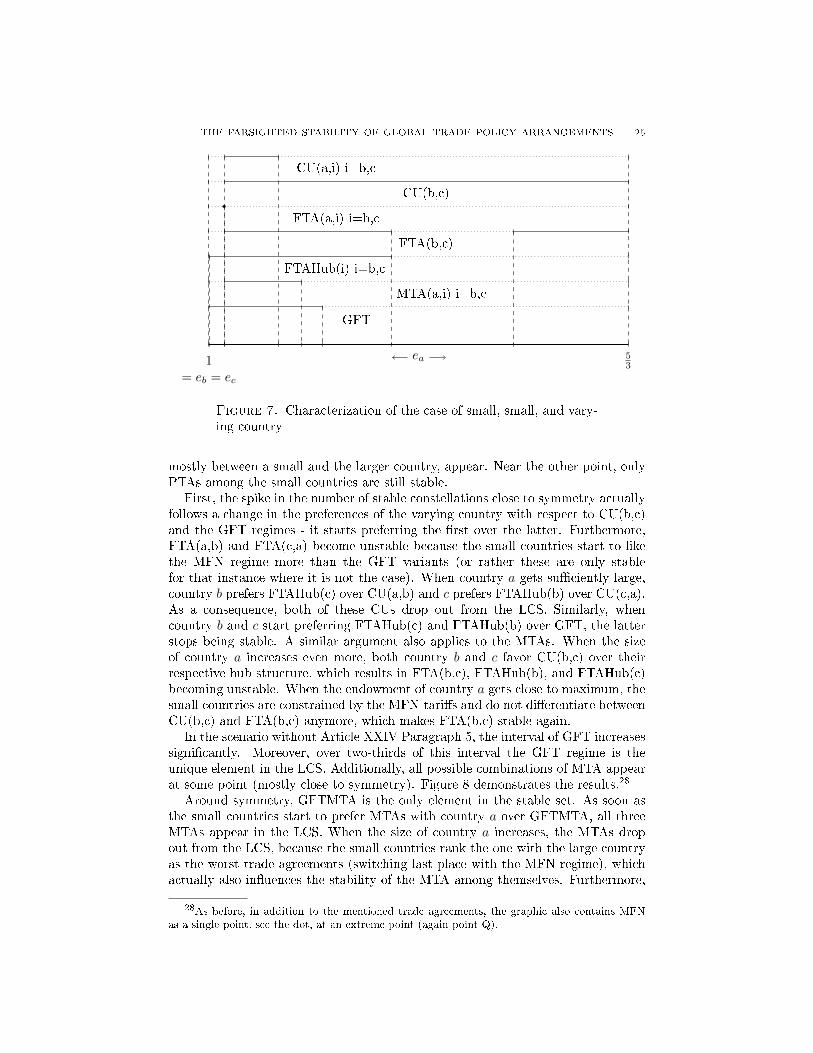
4.3.2. The case of two small, and one varying country. Second, let us show-case the scenario with eb = ec = emin and ea ∈ (emin, emax) (side PQ). In contrastto the previous case, it is not possible to rule out many of the trade agreements.Only MFN, FTAHub(a), and MTA(b,c) never appear in the LCS. The stable set isthen presented in Figure 7.27
In the immediate vicinity around symmetry, the GFT regime is the only elementof the LCS (or rather the group of the three variants forms the stable set), but bothFTAHub(b) and FTAHub(c) emerge as stable outcomes when moving away fromthe extreme point. On the whole interval a number of di�erent PTAs and MTAs,
26In addition to the aforementioned elements, it also pictures MTA(b,c) as a single point, seethe dot, but this appears only for completion sake because that point corresponds to one of theextreme cases (point Q) discussed earlier.
27The dot marks a single point again.
THE FARSIGHTED STABILITY OF GLOBAL TRADE POLICY ARRANGEMENTS 25
CU(a,i) i=b,c
CU(b,c)
FTA(a,i) i=b,c
FTA(b,c)
FTAHub(i) i=b,c
MTA(a,i) i=b,c
GFT
1= eb = ec
53
ea
Figure 7. Characterization of the case of small, small, and vary-ing country
mostly between a small and the larger country, appear. Near the other point, onlyPTAs among the small countries are still stable.
First, the spike in the number of stable constellations close to symmetry actuallyfollows a change in the preferences of the varying country with respect to CU(b,c)and the GFT regimes - it starts preferring the �rst over the latter. Furthermore,FTA(a,b) and FTA(c,a) become unstable because the small countries start to likethe MFN regime more than the GFT variants (or rather these are only stablefor that instance where it is not the case). When country a gets su�ciently large,country b prefers FTAHub(c) over CU(a,b) and c prefers FTAHub(b) over CU(c,a).As a consequence, both of these CUs drop out from the LCS. Similarly, whencountry b and c start preferring FTAHub(c) and FTAHub(b) over GFT, the latterstops being stable. A similar argument also applies to the MTAs. When the sizeof country a increases even more, both country b and c favor CU(b,c) over theirrespective hub structure, which results in FTA(b,c), FTAHub(b), and FTAHub(c)becoming unstable. When the endowment of country a gets close to maximum, thesmall countries are constrained by the MFN-tari�s and do not di�erentiate betweenCU(b,c) and FTA(b,c) anymore, which makes FTA(b,c) stable again.
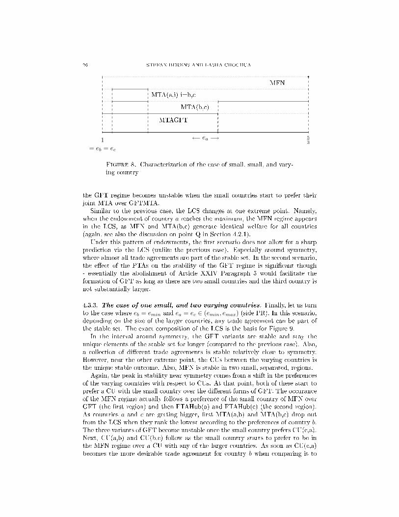
In the scenario without Article XXIV Paragraph 5, the interval of GFT increasessigni�cantly. Moreover, over two-thirds of this interval the GFT regime is theunique element in the LCS. Additionally, all possible combinations of MTA appearat some point (mostly close to symmetry). Figure 8 demonstrates the results.28
Around symmetry, GFTMTA is the only element in the stable set. As soon asthe small countries start to prefer MTAs with country a over GFTMTA, all threeMTAs appear in the LCS. When the size of country a increases, the MTAs dropout from the LCS, because the small countries rank the one with the large countryas the worst trade agreements (switching last place with the MFN regime), whichactually also in�uences the stability of the MTA among themselves. Furthermore,
28As before, in addition to the mentioned trade agreements, the graphic also contains MFNas a single point, see the dot, at an extreme point (again point Q).
26 STEFAN BERENS AND LASHA CHOCHUA
MFN
MTA(a,i) i=b,c
MTA(b,c)
MTAGFT
1= eb = ec
53
ea
Figure 8. Characterization of the case of small, small, and vary-ing country
the GFT regime becomes unstable when the small countries start to prefer theirjoint MTA over GFTMTA.
Similar to the previous case, the LCS changes at one extreme point. Namely,when the endowment of country a reaches the maximum, the MFN regime appearsin the LCS, as MFN and MTA(b,c) generate identical welfare for all countries(again, see also the discussion on point Q in Section 4.2.1).
Under this pattern of endowments, the �rst scenario does not allow for a sharpprediction via the LCS (unlike the previous case). Especially around symmetry,where almost all trade agreements are part of the stable set. In the second scenario,the e�ect of the PTAs on the stability of the GFT regime is signi�cant though- essentially the abolishment of Article XXIV Paragraph 5 would facilitate theformation of GFT as long as there are two small countries and the third country isnot substantially larger.
4.3.3. The case of one small, and two varying countries. Finally, let us turnto the case where eb = emin and ea = ec ∈ (emin, emax) (side PR). In this scenario,depending on the size of the larger countries, any trade agreement can be part ofthe stable set. The exact composition of the LCS is the basis for Figure 9.
In the interval around symmetry, the GFT variants are stable and stay theunique elements of the stable set for longer (compared to the previous case). Also,a collection of di�erent trade agreements is stable relatively close to symmetry.However, near the other extreme point, the CUs between the varying countries isthe unique stable outcome. Also, MFN is stable in two small, separated, regions.
Again, the peak in stability near symmetry comes from a shift in the preferencesof the varying countries with respect to CUs. At that point, both of these start toprefer a CU with the small country over the di�erent forms of GFT. The occuranceof the MFN regime actually follows a preference of the small country of MFN overGFT (the �rst region) and then FTAHub(a) and FTAHub(c) (the second region).As countries a and c are getting bigger, �rst MTA(a,b) and MTA(b,c) drop outfrom the LCS when they rank the lowest according to the preferences of country b.The three variants of GFT become unstable once the small country prefers CU(c,a).Next, CU(a,b) and CU(b,c) follow as the small country starts to prefer to be inthe MFN regime over a CU with any of the larger countries. As soon as CU(c,a)becomes the more desirable trade agreement for country b when comparing it to
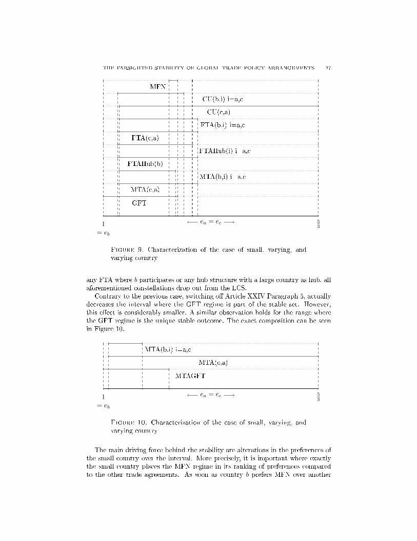
THE FARSIGHTED STABILITY OF GLOBAL TRADE POLICY ARRANGEMENTS 27
MFN
CU(b,i) i=a,c
CU(c,a)
FTA(b,i) i=a,c
FTA(c,a)
FTAHub(i) i=a,c
FTAHub(b)
MTA(b,i) i=a,c
MTA(c,a)
GFT
1= eb
53
ea = ec
Figure 9. Characterization of the case of small, varying, andvarying country
any FTA where b participates or any hub structure with a large country as hub, allaforementioned constellations drop out from the LCS.
Contrary to the previous case, switching o� Article XXIV Paragraph 5, actuallydecreases the interval where the GFT regime is part of the stable set. However,this e�ect is considerably smaller. A similar observation holds for the range wherethe GFT regime is the unique stable outcome. The exact composition can be seenin Figure 10.
MTA(b,i) i=a,c
MTA(c,a)
MTAGFT
1= eb
53
ea = ec
Figure 10. Characterization of the case of small, varying, andvarying country
The main driving force behind the stability are alterations in the preferences ofthe small country over the interval. More precisely, it is important where exactlythe small country places the MFN regime in its ranking of preferences comparedto the other trade agreements. As soon as country b prefers MFN over another
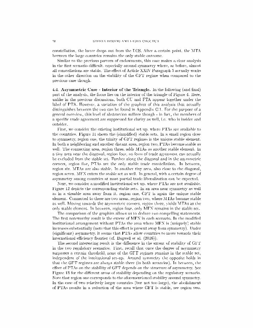
28 STEFAN BERENS AND LASHA CHOCHUA
constellation, the latter drops out from the LCS. After a certain point, the MTAbetween the large countries remains the only stable outcome.
Similar to the previous pattern of endowments, this case makes a clear analysisin the �rst scenario di�cult, especially around symmetry where, as before, almostall constellations are stable. The e�ect of Article XXIV Paragraph 5 actually worksin the other direction on the stability of the GFT regime when compared to theprevious case though.
4.4. Asymmetric Case - Interior of the Triangle. In the following (and �nal)part of the analysis, the focus lies on the interior of the triangle of Figure 4. Here,unlike in the previous discussions, both CU and FTA appear together under thelabel of PTA. However, a variation of the graphics of this analysis that actuallydistinguishes between the two can be found in Appendix C.1. For the purpose of ageneral overview, this level of abstraction su�ces though - in fact, the members ofa speci�c trade agreement are suppressed for clarity as well, i.e. who is insider andoutsider.
First, we consider the existing institutional set-up, where PTAs are available tothe countries. Figure 11 shows the (simpli�ed) stable sets. In a small region closeto symmetry, region one, the trinity of GFT regimes is the unique stable element.In both a neighboring and another distant area, region two, PTAs become stable aswell. The connecting area, region three, adds MTAs as another stable element. Ina tiny area near the diagonal, region four, no form of trade agreement can actuallybe excluded from the stable set. Further along the diagonal and in the asymmetriccorners, region �ve, PTAs are the only stable trade constellation. In between,region six, MTAs are also stable. In another tiny area, also close to the diagonal,region seven, MFN enters the stable set as well. In general, with a certain degree ofasymmetry among countries at most partial trade liberalization can be expected.
Next, we consider a modi�ed institutional set-up, where PTAs are not available.Figure 12 depicts the corresponding stable sets. In an area near symmetry as wellas in a sizeable area away from it, region one, GFT is again the unique stableelement. Connected to these are two areas, region two, where MTAs become stableas well. Moving towards the asymmetric corners, region three, yields MTAs as theonly stable element. In between, region four, only MFN remains in the stable set.
The comparison of the graphics allows us to deduce two compelling statements.The �rst noteworthy result is the extent of MFN in each scenario. In the modi�edinstitutional arrangement without PTAs the area where MFN is (uniquely) stableincreases substantially (note that this e�ect is present away from symmetry). Under(signi�cant) asymmetry, it seems that PTAs allow countries to move towards theirinternational e�ciency frontier (cf. Bagwell et al. (2016)).
The second interesting result is the di�erence in the extent of stability of GFTin the two regulatory scenarios. First, recall that once the degree of asymmetrysurpasses a certain threshold, none of the GFT regimes remains in the stable set,independent of the institutional set-up. Around symmetry the opposite holds inthat the GFT regimes are always stable there (in both scenarios). In between, thee�ect of PTAs on the stability of GFT depends on the structure of asymmetry. SeeFigure 13 for the di�erent areas of stability depending on the regulatory scenario.Note that region one corresponds to the aforementioned stability around symmetry.In the case of two relatively larger countries (but not too large), the abolishmentof PTAs results in a reduction of the area where GFT is stable, see region two.
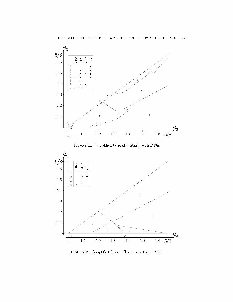
THE FARSIGHTED STABILITY OF GLOBAL TRADE POLICY ARRANGEMENTS 29
MFN
PTA
MTA
GFT
1 x2 x x3 x x x4 x x x x5 x6 x x7 x x x
Figure 11. Simpli�ed Overall Stability with PTAs
MFN
MTA
GFT
1 x2 x x3 x4 x
Figure 12. Simpli�ed Overall Stability without PTAs

30 STEFAN BERENS AND LASHA CHOCHUA
In this instance, PTAs act as `building blocks' on the road to GFT. But whentwo countries are relatively smaller (but not too small), the same regulatory actionyields the exact opposite e�ect, see region three. Here, PTAs are `stumbling blocks'.Thus, whether PTAs are `building blocks' or `stumbling blocks' in the vicinity ofsymmetry depends on the relative size of the majority of the countries.
I II1 x x2 x3 x
Figure 13. The di�erent areas of stability of the GFT regime inthe scenario with (I) and without (II) PTAs
In a nutshell: If the world is in the vicinity of symmetry and two out of threecountries are close to identical while relatively smaller than the other one, the areawhere the GFT regime is stable increases when prohibiting PTAs. However, whentwo similar countries are relatively larger, the availability of PTAs is conducive tothe stability of the GFT regime. Finally, if the world is further away from symmetry,full trade liberalization is not attainable at all and an area where the MFN regimeis stable appears in the scenario without PTAs.
5. Discussion
In this section, let us �rst compare the �ndings of our paper with those of severalsimilar studies and underline the di�erences in the modeling strategies, especiallywith respect to the explanatory power of each approach. Second, this section linksour predictions to di�erent empirical observations, thereby validating our approach.
THE FARSIGHTED STABILITY OF GLOBAL TRADE POLICY ARRANGEMENTS 31
Let us start with the paper of Saggi, Woodland and Yildiz (2013).29 First notethat the underlying trade model in our paper is similar to theirs, which allows adirect comparison of the �ndings in certain scenarios (found in the next paragraph).The �rst distinction is the set of trade agreements under consideration. While inour model countries can be involved in multilateral trade liberalization via MTAs orthey may choose to carry out their favored form of preferential trade liberalizationthrough CUs or FTAs, Saggi, Woodland and Yildiz (2013) focuses on two out ofthese three possibilities, namely CUs and MTAs. In our opinion, the expanded setof trade arrangements in our model allows us to fully capture the trade-o�s amongthe alternatives and make the model realistic. The second signi�cant di�erence isthe concept of stability. While our framework uses the notion of LCS, the paperof Saggi, Woodland and Yildiz (2013) utilizes Coalition-Proof Nash Equilibria. AsBernheim, Peleg and Whinston (1987) note, their notion of self-enforceability, whichis critical for Coalition-Proof Nash Equilibria, is too restrictive in one crucial aspect,mainly: `When a deviation occurs, only members of the deviating coalition maycontemplate deviations from the deviation. This rules out the possibility that somemember of the deviating coalition might form a pact to deviate further with someonenot included in this coalition.' Importantly, this limitation does not a�ect theconcept of LCS. It is not a pure academic di�erence. The historic developmentof the two (disjoint) trade constellations in Europe in the 1960s, the EuropeanEconomic Community (EEC) and the European Free Trade Association (EFTA),can not be captured by a model using Coalition-Proof Nash Equilibria, because itexcludes those strategies that the UK actually followed during that time.30 Whilebeing a member of EFTA the UK applied for EEC membership in 1961 and therebyundermined the stability of the EFTA. Furthermore, `the more ambitious KennedyRound between 1964 and 1967 coincided with negotiations to expand the EEC toinclude Britain, Ireland, Denmark, Greece, and Norway - and was motivated inpart by US concerns about being excluded from an ever-broader and more uni�edEuropean market.` (World Trade Report 2011). Thus, unlike the Coalition-ProofNash Equilibrium, the LCS allows interactions among members and non-membersof coalitions simultaneously, thereby accommodating these historic developments.Additionally, the (conjectured) motivation of the US reinforces the importance ofthe interaction among di�erent modes and forms of trade liberalization.
In speci�c cases it is actually possible to directly compare the composition of thestable sets of our paper with those of Saggi, Woodland and Yildiz (2013). In fact,their `multilateralism game' �ts our scenario of a modi�ed institutional arrangementwithout PTAs. Compare Figures 2 and 5 of Saggi, Woodland, and Yildiz (2013)with Figures 10 and 8 in our paper correspondingly. In the case with one smallcountry and the other two varying, both approaches predict the same stable setsnear the endpoints of the interval. In our paper GFT stays part of the stable seteven when MTAs, either between the large countries or a small and a large country,become stable as well - which is in contrast to Saggi, Woodland, and Yildiz (2013).A similar observation follows for the case of two small and one varying country, i.e.
29As mentioned in Section 2, this paper analyzes the case of CUs and MTA while their otherpapers (Saggi and Yildiz (2010) resp. Missions, Saggi and Yildiz (2016)) focus on di�erent combi-nations of trade agreements (FTAs and MTAs resp. CUs and FTAs) but use a similar framework.As a consequence, the comparison of methodology applies to these papers as well.
30See Baldwin and Gylfason (1995).
32 STEFAN BERENS AND LASHA CHOCHUA
near the endpoints of the interval results coincide while the appearance of MTAsdoes not prevent GFT from staying in the stable set. Furthermore, in our modelthere exists an interval where GFT becomes the unique stable element once more.It seems that one e�ect of the unlimited farsightedness is the proliferation of GFT.
Another relevant paper is that of Lake (2017). Apart from the stability concept,the approach of Lake also di�ers with respect to the choice set. There, the focus lieson FTAs. In this respect, a direct comparison of the �ndings is di�cult. Moreover,compared to the previous paper, the `multilateralism game' is further simpli�ed inLake (2017), as the only possible regime there is the three country constellation thatresults in GFT. Furthermore, as the underlying trade model, the paper employsthe political economy oligopolistic model. However, according to the paper, the�ndings are robust with respect to various underlying trade models, including thecompetition via exports model. Additionally, Lake himself compares his results tothose of Saggi and Yildiz (2010). Due to the similarity of the `multilateralism game'in Saggi and Yildiz (2010) and Saggi, Woodland, and Yildiz (2013), it is only logicalto compare our results with those of Lake (2017) as with the previous paper.
According to Lake (2017), speci�cally Figure 3, the exact role of FTAs underasymmetry depends on the nature of asymmetry (similar to our �ndings). However,the direction of the e�ect of PTAs on trade liberalization is the opposite. There, incase of two larger and one small country, FTAs act as `(strong) stumbling blocs', andwith two smaller and one larger country, as `(strong) building blocs'. Furthermore,there it seems that the determining factor are the preferences of the larger countries,while in our case the �ndings are driven by the preferences of the smaller countries.Thus, the aforementioned di�erences in the choice set and stability concept appearto shift the power to in�uence the negotiations among the countries, which thenproduces a di�erent outcome. Speci�cally, in the case of the `multilateralism game',which corresponds to our scenario without PTA, there are essentially two areas, thatis one where GFT emerges as unique equilibrium and one with MFN instead. In theparameter space triangle the �rst makes up the upper left part of the triangle, whilethe second makes up the opposing lower right.31 Therefore, for two larger countriesthe GFT regime remains the unique equilibrium for the whole interval, whereas inour model it only stays stable in the vicinity of symmetry (only partially unique)and then the MTA between the larger countries is the unique stable outcome, asseen in Figure 10. Furthermore, for two smaller countries �rst GFT then MFNis the unique equilibrium, while in the beginning GFT is also stable in our case(although only partially unique) the MTA between the small countries takes itplace as the unique stable element near the end, depicted in Figure 8. Finally, inthe case of three di�erent countries, it starts with MFN and ends with GFT as theunique equilibrium, which corresponds to our �ndings for the �rst part but thenin the second part the MTA between the medium and large country is the uniquestable element, visible in Figure 6.
Another aspect of Lake (2017) necessitates a remark, namely the assumption thata once created trade agreement remains binding from then on. Lake argues that`the binding nature of trade agreements is pervasive in the literature and realistic'.However, the latest developments in the world cast doubt on this plausibility. TheUSA, for example, pulled out of the negotiations for the Trans-Paci�c Partnership
31The �rst corresponds to the regions denoted WBB and SSB in Figure 3 of Lake (2017), whilethe second matches the regions SBB and WSB.
THE FARSIGHTED STABILITY OF GLOBAL TRADE POLICY ARRANGEMENTS 33
at the �nal stage and currently negotiates with South Korea to amend the so-called KORUS FTA. The developments around `Brexit' are another argument formodeling non-binding trade agreements. Using the LCS as stability concept allowedus to accommodate such deviations.
A �nal remark on the relation of our research with empirical observations. Asthe analysis has shown, a growing degree of asymmetry among countries produceda signi�cant area of stability for the MFN regime when PTAs are prohibited, seeregion four in Figure 12. If one would interpret the expansion of the WTO rule setto an increasing number of countries as an ampli�cation of asymmetry among itsmember states, then the potential of PTAs to prevent the MFN regime might beone of the driving factors of the prevalence of PTAs in recent history. However, theWorld Trade Report (2011) casts doubt on this motive. According to the report:`Approximately 66 per cent of tari� lines with MFN rates above 15 percentagepoints have not been reduced in PTAs.' Note that a reduction of the tari� peaksfor 34 percent of the tari� lines is still a signi�cant e�ect considering the fact thatthe majority of tari� peaks occurs in agricultural and labor-intensive manufacturingsectors, which are politically sensitive and countries usually try to exclude themfrom the trade liberalization via PTAs. Furthermore, according to the same report,over time more and more PTAs have included provisions regarding technical barriersto trade - a category of the Non-Tari� Barriers (NTBs). The paper of Kee, Nicita,and Olarreaga (2009) estimates that restrictiveness measures that include NTBsare on average about 87 percent higher than the measures based on tari�s alone.Thus, in order to evaluate the aforementioned motive properly, the e�ects of NTBsshould be included in the analysis as well. Moreover, contrary to the conclusionof the report that `preference margins are small and market access is unlikely inmany cases to be an important reason for creating new PTAs', Keck and Lendle(2012) show that the preferential utilization rates are often high even in the caseof small preference margins and they increase both with the preference margin andthe export volume. All in all, it is our opinion that there is (partial) evidence forthe motive of avoidance of MFN via PTAs which coincides with the predictions ofour model about the trade-o� between trade liberalization and the MFN regime inthe asymmetric part of the parameter space.
As this overview showed, a number of core attributes of the LCS, speci�callythe farsightedness, the non-binding nature of agreements, and the possibility ofinteractions between members and non-members of coalitions, capture importantmechanisms present in the world and in�uence the composition of the stable setsigni�cantly (when compared to other stability concepts).
6. Conclusion
Under the rules of the WTO (previously GATT), a group of countries can engagein both multilateral and preferential trade liberalization. The formation of globaltrade agreements is a complex game and the rules of the game in�uence the natureof the exact outcomes. WTO's Article I aims at creating the global free tradesystem, while Article XXIV Paragraph 5 allows countries to seemingly circumventthe liberalization process. In this paper, our focus lies on the stability of trade policyarrangements under two di�erent regulatory scenarios (with and without PTAs)assuming unlimited farsightedness of the participants in the trade negotiations andconsidering an extensive set of trade agreements - moving our model closer to reality.
34 STEFAN BERENS AND LASHA CHOCHUA
Unfortunately, the answer to the question whether PTAs are `building blocks' or`stumbling blocks' on the path towards global free trade is not as straightforwardas one would like it to be. In the end, the results presented here are mixed anddepend on the size distribution of the countries. Under symmetry, GFT is theunique stable trade constellation in both regulatory scenarios. But as soon as onemoves away from symmetry, GFT might not be reached at all. In between, the e�ectof switching o� Article XXIV Paragraph 5 depends on the exact asymmetry. In casetwo countries are relatively smaller, prohibiting PTAs increases the area of stabilityof the GFT regimes. When two countries are relatively larger, it reduces the area.Once the world is further away from symmetry, abolishing the exception for PTAsmight result in the worst possible state from the perspective of overall world welfare,the non-cooperative MFN regime. Therefore, under such circumstances, PTAs actas a mechanism that prevents the MFN regime.
Our research also raises a couple of questions in need of further investigation.First, it would be interesting to study the robustness of the �ndings with respect tothe underlying trade model. While the model of competition via exports remainspopular in the related literature, economists also extensively use both oligopolyand competition via imports model. Fortunately, the framework presented heredoes allow for a di�erent underlying trade model such as the ones mentioned above.Another potential area of inquiry might be an extension of the framework to increasethe number of countries. Nowadays, in addition to bilateral negotiations, so-calledplurilateral negotiations play an important role in the development of preferentialtrade liberalization. Recent examples are the Trans-Paci�c Partnership (TTP) andthe Regional Comprehensive Economic Partnership (RCEP). Including more thanthree countries in a model would allow us to investigate the strategic interactionsamong countries whilst taking these negotiations into account. The introduction ofpolitical economy considerations to the underlying trade model is another area ofinterest32, as it might allow us to understand the nature of tari� peaks occurringafter PTAs come into e�ect. It is our opinion that modi�cations or extensions ofour framework (as mentioned here) are directions worthy of further research.
As a �nal remark, it is perhaps important, going forward, to move the debateof `building blocks' vs. `stumbling blocks' to a level of detail that goes beyond thisbinary choice.
References
[1] General agreement on tari�s and trade, 1947. Source: http://www.wto.org.[2] World trade report 2011, 2011. Source: http://www.wto.org.[3] Philippe Aghion, Pol Antràs, and Elhanan Helpman. Negotiating free trade. Journal of In-
ternational Economics, 73(1):1�30, 2007.[4] Robert Aumann and Roger Myerson. Endogenous formation of links between players and
coalitions: an application of the shapley value. The Shapley Value, pages 175�191, 1988.[5] Kyle Bagwell, Chad P. Bown, and Robert W. Staiger. Is the wto passé? Journal of Economic
Literature, 54(4):1125�1231, December 2016.[6] Kyle Bagwell and Robert W. Staiger. Regionalism and multilateral tari� cooperation. Work-
ing Paper 5921, National Bureau of Economic Research, February 1997.[7] Kyle Bagwell and Robert W Staiger. The design of trade agreements. Handbook of Commer-
cial Policy, 1:435�529, 2016.[8] Richard E. Baldwin and Thorvaldur Gylfason. A domino theory of regionalism. In Expanding
Membership of the European Union, pages 25�53. Cambridge University Press, 1995.
32See for example Facchini et al. (2013).
THE FARSIGHTED STABILITY OF GLOBAL TRADE POLICY ARRANGEMENTS 35
[9] B. Douglas Bernheim, Bezalel Peleg, and Michael Whinston. Coalition-proof nash equilibriai. concepts. Journal of Economic Theory, 42(1):1�12, 1987.
[10] Jagdish Bhagwati. Regionalism and multilateralism: an overview. New dimensions in regional
integration, 22:51, 1993.[11] Michael Suk-Young Chwe. Farsighted coalitional stability. Journal of Economic Theory,
63(2):299 � 325, 1994.[12] Giovanni Facchini, Peri Silva, and Gerald Willmann. The customs union issue: Why do we
observe so few of them? Journal of International Economics, 90(1):136 � 147, 2013.[13] Taiji Furusawa and Hideo Konishi. Free trade networks. Journal of International Economics,
72(2):310�335, 2007.[14] Sanjeev Goyal and Sumit Joshi. Bilateralism and free trade. International Economic Review,
47(3):749�778, 2006.[15] Gene M Grossman. The purpose of trade agreements. Handbook of Commercial Policy, 1:379�
434, 2016.[16] John Harsanyi. An equilibrium-point interpretation of stable sets and a proposed alternative
de�nition. Management Science, 20(11):1472�1495, 1974.[17] P. Jean-Jacques Herings, Ana Mauleon, and Vincent Vannetelbosch. Farsightedly stable net-
works. Games and Economic Behavior, 67(2):526�541, 2009.[18] P.J.J. Herings, A. Mauleon, and V. Vannetelbosch. Stability of networks under level-k far-
sightedness. Research Memorandum 030, Maastricht University, Graduate School of Businessand Economics (GSBE), January 2014.
[19] Matthew O Jackson and Asher Wolinsky. A strategic model of social and economic networks.Journal of economic theory, 71(1):44�74, 1996.
[20] Alexander Keck and Andreas Lendle. New evidence on preference utilization. WTO Sta�Working Papers ERSD-2012-12, World Trade Organization (WTO), Economic Research andStatistics Division, September 2012.
[21] Hiau Looi Kee, Alessandro Nicita, and Marcelo Olarreaga. Estimating trade restrictivenessindices. The Economic Journal, 119(534):172�199, 2009.
[22] James Lake. Free trade agreements as dynamic farsighted networks. Economic Inquiry,55(1):31�50, 2017.
[23] Giovanni Maggi. International trade agreements. In Handbook of International Economics,volume 4, chapter 6, pages 317�390. 2014.
[24] Paul Missios, Kamal Saggi, and Halis Murat Yildiz. External trade diversion, exclusion incen-tives and the nature of preferential trade agreements. Journal of International Economics,99:105�119, 2016.
[25] Kamal Saggi, Alan Woodland, and Halis Murat Yildiz. On the relationship between prefer-ential and multilateral trade liberalization: the case of customs unions. American Economic
Journal: Microeconomics, 5(1):63�99, 2013.[26] Kamal Saggi and Halis Murat Yildiz. Bilateralism, multilateralism, and the quest for global
free trade. Journal of International Economics, 81(1):26�37, 2010.[27] John von Neumann and Oskar Morgenstern. Theory of Games and Economic Behavior.
Princeton University Press, 1944.[28] Jin Zhang, Zhiwei Cui, and Lei Zu. The evolution of free trade networks. Journal of Economic
Dynamics and Control, 38:72�86, 2014.[29] Jin Zhang, Licun Xue, and Lei Zu. Farsighted free trade networks. International Journal of
Game Theory, 42(2):375�398, 2013.

36 STEFAN BERENS AND LASHA CHOCHUA
Appendix A. Pseudocode
Note, that a couple of functions and variables are directly baked into the programwithout any further explanation in the pseudocode below - for example the matrixthat determines the general network structure (for each player and all coalitions).The origin and characterization of these can be found in their respective parts inthe main paper. The network structure A and the preference relations B both enteras a collection of |X| × |X|-matrices, {AS}S⊆N,S 6=∅ and {BS}S⊆N,S 6=∅ resp., where(AS)i,j = 1{i→Sj}(i, j) and (BS)i,j = 1{i≺Sj}(i, j) for (i, j) ∈ X ×X.
Algorithm Largest Consistent Set
Input: Countries N , Outcomes X, Network Structure A, Preference Relations BOutput: Largest Consistent Set {Y }1: procedure ParameterSpaceLCS(N,X,A,B)2: E = eMaxArea . See Section 3.63: α = αMinV alue(E) . See Section 3.64: for e ∈ E do
5: Y = GeneralLCS(N,X,A,B)
6: return {Y }
7: function GeneralLCS(N,X,A,B)8: for S ⊆ N do
9: CS = min{AS , BS}10: D0 = maxS⊆N{CS} . : Direct Dominance11: n = 012: repeat
13: n = n+ 114: for S ⊆ N do
15: AnS = (1{(AS ·Dn−1)i,j 6=0}(i, j))(i,j)∈X×X
16: DnS = min{An
S , BS}17: Dn = maxS⊆N{Dn
S} . : Indirect Dominance18: until Dn = Dn−1
19: D = 1X +Dn
20: Y 0 = (1)x∈X21: m = 022: repeat
23: m = m+ 124: for x ∈ X do
25: if Y m−1x = 0 then
26: Y mx = 0
27: else
28: y = maxk∈X,S⊆N
{(AS)x,k
(1−max
z∈X
{Y m−1z (D)k,z (1− (BS)x,z)
})}29: Y m
x = Y m−1x − y
30: until Y m = Y m−1
31: Y = Y m
32: return Y
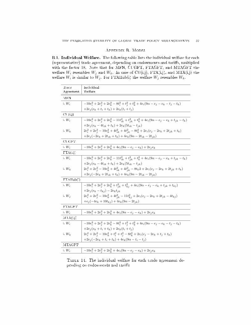
THE FARSIGHTED STABILITY OF GLOBAL TRADE POLICY ARRANGEMENTS 37
Appendix B. Model
B.1. Individual Welfare. The following table lists the individual welfare for each(representative) trade agreement, depending on endowments and tari�s, multipliedwith the factor 18. Note that for MFN, CUGFT, FTAGFT, and MTAGFT thewelfare Wi resembles Wj and Wk. In case of CU(i,j), FTA(i,j), and MTA(i,j) thewelfare Wi is similar to Wj . For FTAHub(i) the welfare Wj resembles Wk.
Trade IndividualAgreement Welfare
MFN
�
Wi −10e2i + 2e2j + 2e2k − 8t2i + t2j + t2k + 4ei(9α− ej − ek − tj − tk)
+2ej(ek + ti + tk) + 2ek(ti + tj)
CU(i,j)
�
Wi −10e2i + 2e2j + 2e2k − 11t2ik + t2jk + t2k + 4ei(9α− ej − ek + tjk − tk)
+2ej(ek − 4tik + tk) + 2ek(5tik − tjk)
�
Wk 2e2i + 2e2j − 10e2k + 4t2ik + 4t2jk − 8t2k + 2ei(ej − 2ek + 2tjk + tk)
+2ej(−2ek + 2tik + tk) + 4ek(9α− 2tik − 2tjk)
CUGFT
�
Wi −10e2i + 2e2j + 2e2k + 4ei(9α− ej − ek) + 2ejek
FTA(i,j)
�
Wi −10e2i + 2e2j + 2e2k − 11t2ik + t2jk + t2k + 4ei(9α− ej − ek + tjk − tk)
+2ej(ek − 4tik + tk) + 2ek(5tik − tjk)
�
Wk 2e2i + 2e2j − 10e2k + 4t2ik + 4t2jk − 8tk2 + 2ei(ej − 2ek + 2tjk + tk)
+2ej(−2ek + 2tik + tk) + 4ek(9α− 2tik − 2tjk)
FTAHub(i)
�
Wi −10e2i + 2e2j + 2e2k + t2jk + t2kj + 4ei(9α− ej − ek + tjk + tkj)
+2ej(ek − tkj)− 2ektjk
�
Wj 2e2i + 2e2j − 10e2k + 4t2jk − 11t2kj + 2ei(ej − 2ek + 2tjk − 4tkj)
+ej(−4ek + 10tkj) + 4ek(9α− 2tjk)
FTAGFT
�
Wi −10e2i + 2e2j + 2e2k + 4ei(9α− ej − ek) + 2ejek
MTA(i,j)
�
Wi −10e2i + 2e2j + 2e2k − 8t2i + t2j + t2k + 4ei(9α− ej − ek − tj − tk)
+2ej(ek + ti + tk) + 2ek(ti + tj)
�
Wk 2e2i + 2e2j − 10e2k + t2i + t2j − 8t2k + 2ei(ej − 2ek + tj + tk)
+2ej(−2ek + ti + tk) + 4ek(9α− ti − tj)
MTAGFT
�
Wi −10e2i + 2e2j + 2e2k + 4ei(9α− ej − ek) + 2ejek
Table 14. The individual welfare for each trade agreement de-pending on endowments and tari�s

38 STEFAN BERENS AND LASHA CHOCHUA
B.2. Tari�s. The following describes the tari�s that the countries choose for eachtrade agreement. In addition to the speci�c restrictions mentioned in Section 3.3,all tari�s are bounded both from below and above by zero and the MFN-tari�respectively. As per WTO rule, the formation of any PTA does not allow additionaltari�s towards others - which results in the upper bound of the MFN-tari�. Also,any form of subsidies is excluded here - which results in the lower bound of zero.Now, the following determines and describes the optimal tari�s for each scenarioand the cases where capping occurs:
B.2.1. MFN. In this case, the optimal tari� of country i, given by t∗i = 18 (ej + ek),
is always greater than zero as the endowments themselves are greater than zero.Additionally, t∗i is going to play the role of the maximal tari� for country i for allthe other agreements, then denoted tMFN
i .
B.2.2. CU. Consider the scenario CU(i,j), then the optimal tari� of country i to-wards country k, given by t∗ik = 1
5 (2ek − ej), is always greater than zero but notalways less than the MFN-tari� (and the one towards country j, t∗ij , is always zero):
i) Lower Bound. By assumption on the endowments ek ≥ 35ej and thus ek >
12ej ,
which guarantees t∗ik > 0.ii) Upper Bound. By assumption on the endowments ek ≤ 5
3ej however t∗ik ≤ tMFN
i
requires ek ≤ 1311ej , which leaves the interval 13
11ej < ek ≤ 53ej to require capping.
For this interval, the (maximal) MFN-tari� is optimal as the derivative of the jointwelfare with respect to tik is always greater than zero on the interval [0, tMFN
i ]:
∂(Wi +Wj)
tik=
1
9(−10tik − 2ej + 4ek) ≥ 1
36(−13ej + 11ek) > 0
B.2.3. FTA. Consider the scenario FTA(i,j), then the optimal tari� of country itowards country k, given by t∗ik = 1
11 (5ek−4ej), is neither always greater than zeronor always less than the MFN-tari� (but the one towards country j, t∗ij , is zero):
i) Lower Bound. By assumption on the endowments ek ≥ 35ej however t∗ik ≥ 0
requires ek ≥ 45ej , which leaves the interval 3
5ej ≤ ek <45ej to require capping.
For this interval, the (minmal) zero-tari� is optimal as the derivative of the welfarewith respect to tik is always lesser than zero on the interval [0, tMFN
i ]:
∂Wi
∂tik=
1
9(−11tik − 4ej + 5ek) ≤ 1
9(5ek − 4ej) < 0
ii) Upper Bound. By assumption on the endowments ek ≤ 53ej however t
∗ik ≤ tMFN
i
requires ek ≤ 4329ej , which leaves the interval 43
29ej < ek ≤ 53ej to require capping.
For this interval, the (maximal) MFN-tari� is optimal as the derivative of thewelfare with respect to tik is always greater than zero on the interval [0, tMFN
i ]:
∂Wi
∂tik=
1
9(−11tik − 4ej + 5ek) ≥ 1
72(−43ej + 29ek) > 0
B.2.4. MTA. Consider the scenario MTA(i,j), then the optimal tari� of country i,given by t∗i = 1
7 (2ek − ej), is greater than zero and less or equal to the MFN-tari�
as per assumption on the endowments 35ej ≤ ek ≤
53ej .
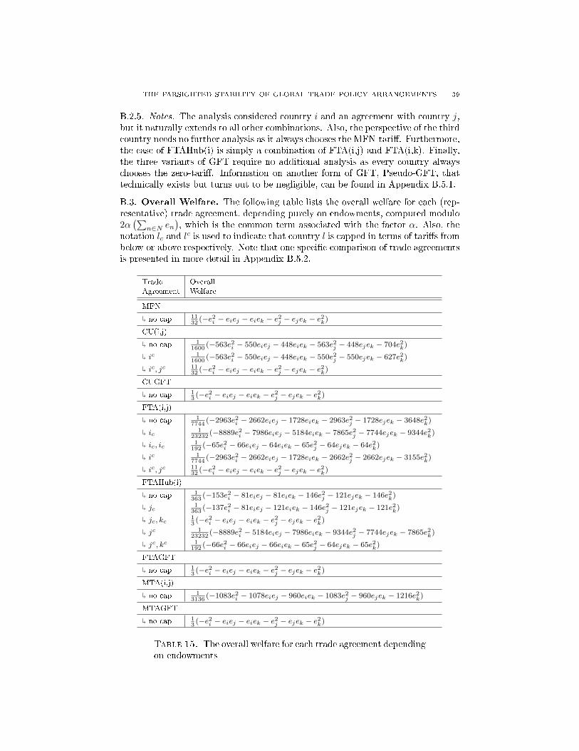
THE FARSIGHTED STABILITY OF GLOBAL TRADE POLICY ARRANGEMENTS 39
B.2.5. Notes. The analysis considered country i and an agreement with country j,but it naturally extends to all other combinations. Also, the perspective of the thirdcountry needs no further analysis as it always chooses the MFN-tari�. Furthermore,the case of FTAHub(i) is simply a combination of FTA(i,j) and FTA(i,k). Finally,the three variants of GFT require no additional analysis as every country alwayschooses the zero-tari�. Information on another form of GFT, Pseudo-GFT, thattechnically exists but turns out to be negligible, can be found in Appendix B.5.1.
B.3. Overall Welfare. The following table lists the overall welfare for each (rep-resentative) trade agreement, depending purely on endowments, computed modulo2α(∑
n∈N en), which is the common term associated with the factor α. Also, the
notation lc and lc is used to indicate that country l is capped in terms of tari�s from
below or above respectively. Note that one speci�c comparison of trade agreementsis presented in more detail in Appendix B.5.2.
Trade OverallAgreement Welfare
MFN
�
no cap 1132
(−e2i − eiej − eiek − e2j − ejek − e2k)
CU(i,j)
�
no cap 11600
(−563e2i − 550eiej − 448eiek − 563e2j − 448ejek − 704e2k)
�
ic 11600
(−563e2i − 550eiej − 448eiek − 550e2j − 550ejek − 627e2k)
�
ic, jc 1132
(−e2i − eiej − eiek − e2j − ejek − e2k)
CUGFT
�
no cap 13
(−e2i − eiej − eiek − e2j − ejek − e2k)
FTA(i,j)
�
no cap 17744
(−2963e2i − 2662eiej − 1728eiek − 2963e2j − 1728ejek − 3648e2k)
�
ic1
23232(−8889e2i − 7986eiej − 5184eiek − 7865e2j − 7744ejek − 9344e2k)
�
ic, ic1
192(−65e2i − 66eiej − 64eiek − 65e2j − 64ejek − 64e2k)
�
ic 17744
(−2963e2i − 2662eiej − 1728eiek − 2662e2j − 2662ejek − 3155e2k)
�
ic, jc 1132
(−e2i − eiej − eiek − e2j − ejek − e2k)
FTAHub(i)
�
no cap 1363
(−153e2i − 81eiej − 81eiek − 146e2j − 121ejek − 146e2k)
�
jc1
363(−137e2i − 81eiej − 121eiek − 146e2j − 121ejek − 121e2k)
�
jc, kc13
(−e2i − eiej − eiek − e2j − ejek − e2k)
�
jc 123232
(−8889e2i − 5184eiej − 7986eiek − 9344e2j − 7744ejek − 7865e2k)
�
jc, kc 1192
(−66e2i − 66eiej − 66eiek − 65e2j − 64ejek − 65e2k)
FTAGFT
�
no cap 13
(−e2i − eiej − eiek − e2j − ejek − e2k)
MTA(i,j)
�
no cap 13136
(−1083e2i − 1078eiej − 960eiek − 1083e2j − 960ejek − 1216e2k)
MTAGFT
�
no cap 13
(−e2i − eiej − eiek − e2j − ejek − e2k)
Table 15. The overall welfare for each trade agreement dependingon endowments
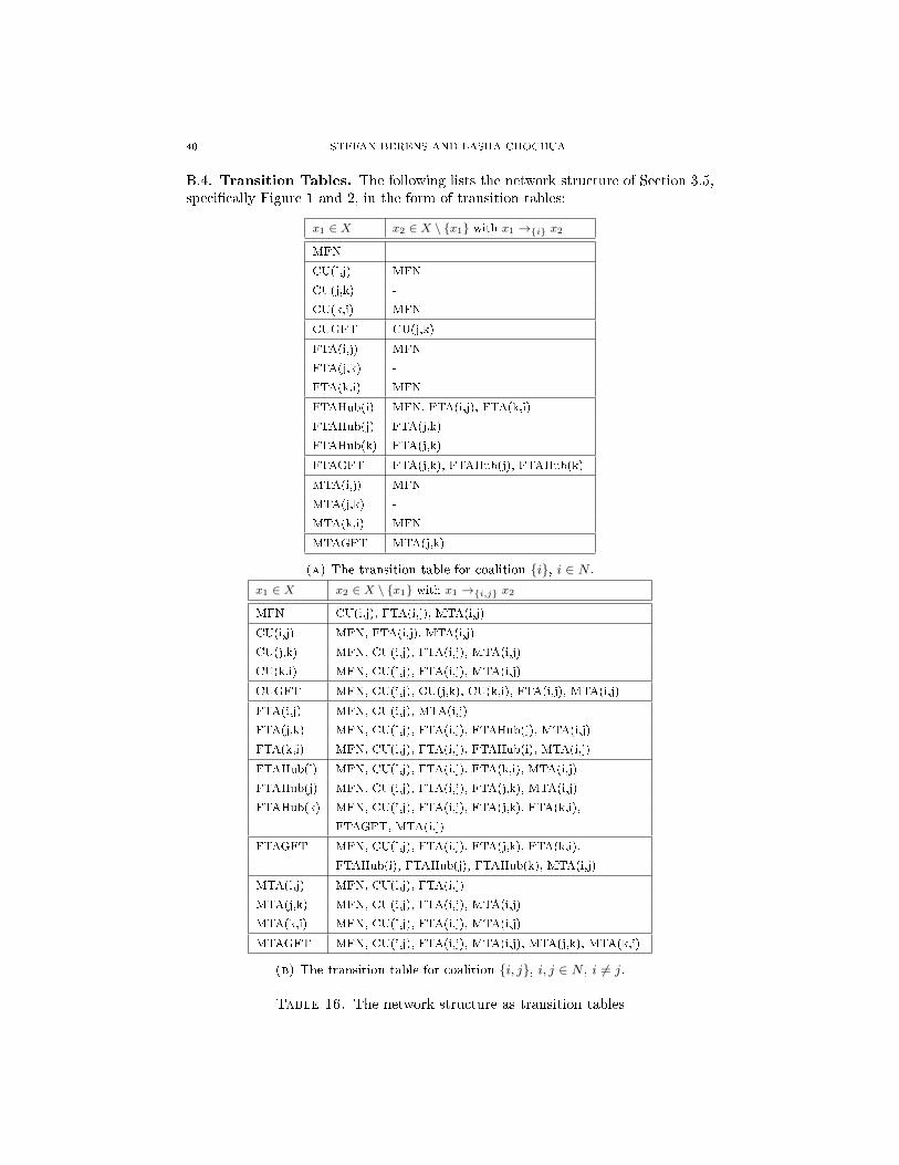
40 STEFAN BERENS AND LASHA CHOCHUA
B.4. Transition Tables. The following lists the network structure of Section 3.5,speci�cally Figure 1 and 2, in the form of transition tables:
x1 ∈ X x2 ∈ X \ {x1} with x1 →{i} x2
MFN -
CU(i,j) MFN
CU(j,k) -
CU(k,i) MFN
CUGFT CU(j,k)
FTA(i,j) MFN
FTA(j,k) -
FTA(k,i) MFN
FTAHub(i) MFN, FTA(i,j), FTA(k,i)
FTAHub(j) FTA(j,k)
FTAHub(k) FTA(j,k)
FTAGFT FTA(j,k), FTAHub(j), FTAHub(k)
MTA(i,j) MFN
MTA(j,k) -
MTA(k,i) MFN
MTAGFT MTA(j,k)
(a) The transition table for coalition {i}, i ∈ N .
x1 ∈ X x2 ∈ X \ {x1} with x1 →{i,j} x2
MFN CU(i,j), FTA(i,j), MTA(i,j)
CU(i,j) MFN, FTA(i,j), MTA(i,j)
CU(j,k) MFN, CU(i,j), FTA(i,j), MTA(i,j)
CU(k,i) MFN, CU(i,j), FTA(i,j), MTA(i,j)
CUGFT MFN, CU(i,j), CU(j,k), CU(k,i), FTA(i,j), MTA(i,j)
FTA(i,j) MFN, CU(i,j), MTA(i,j)
FTA(j,k) MFN, CU(i,j), FTA(i,j), FTAHub(j), MTA(i,j)
FTA(k,i) MFN, CU(i,j), FTA(i,j), FTAHub(i), MTA(i,j)
FTAHub(i) MFN, CU(i,j), FTA(i,j), FTA(k,i), MTA(i,j)
FTAHub(j) MFN, CU(i,j), FTA(i,j), FTA(j,k), MTA(i,j)
FTAHub(k) MFN, CU(i,j), FTA(i,j), FTA(j,k), FTA(k,i),
FTAGFT, MTA(i,j)
FTAGFT MFN, CU(i,j), FTA(i,j), FTA(j,k), FTA(k,i),
FTAHub(i), FTAHub(j), FTAHub(k), MTA(i,j)
MTA(i,j) MFN, CU(i,j), FTA(i,j)
MTA(j,k) MFN, CU(i,j), FTA(i,j), MTA(i,j)
MTA(k,i) MFN, CU(i,j), FTA(i,j), MTA(i,j)
MTAGFT MFN, CU(i,j), FTA(i,j), MTA(i,j), MTA(j,k), MTA(k,i)
(b) The transition table for coalition {i, j}, i, j ∈ N , i 6= j.
Table 16. The network structure as transition tables
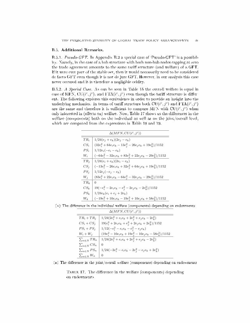
THE FARSIGHTED STABILITY OF GLOBAL TRADE POLICY ARRANGEMENTS 41
B.5. Additional Remarks.
B.5.1. Pseudo-GFT. In Appendix B.2 a special case of `Pseudo-GFT' is a possibil-ity. Namely, in the case of a hub structure with both non-hub nodes capping at zerothe trade agreement amounts to the same tari� structure (and welfare) of a GFT.If it were ever part of the stable set, then it would necessarily need to be consideredde facto GFT even though it is not de jure GFT. However, in our analysis this casenever occured and it is therefore a negligible oddity.
B.5.2. A Special Case. As can be seen in Table 15 the overall welfare is equal incase of MFN, CU(ic, jc), and FTA(ic, jc) even though the tari� structure is di�er-ent. The following explores this equivalence in order to provide an insight into theunderlying mechanics. In terms of tari� structure both CU(ic, jc) and FTA(ic, jc)are the same and therefore it is su�cient to compare MFN with CU(ic, jc) whenonly interested in (e�ects on) welfare. Now, Table 17 shows us the di�erences in thewelfare (components) both on the individual as well as on the joint/overall level,which are computed from the expressions in Table 18 and 19.
∆(MFN,CU(ic, jc))
TRi 1/24(ej + ek)(2ej − ek)
CSi (32e2i + 64eiek − 13e2j − 26ejek + 19e2k)/1152
PSi 1/12ei(−ei − ek)
Wi (−64e2i − 32eiek + 83e2j + 22ejek − 29e2k)/1152
TRj 1/24(ei + ek)(2ei − ek)
CSj (−13e2i − 26eiek + 32e2j + 64ejek + 19e2k)/1152
PSj 1/12ej(−ej − ek)
Wj (83e2i + 22eiek − 64e2j − 32ejek − 29e2k)/1152
TRk 0
CSk 19(−e2i − 2eiek − e2j − 2ejek − 2e2k)/1152
PSk 1/24ek(ei + ej + 2ek)
Wk (−19e2i + 10eiek − 19e2j + 10ejek + 58e2k)/1152
(a) The di�erence in the individual welfare (components) depending on endowments
∆(MFN,CU(ic, jc))
TRi + TRj 1/24(2e2i + eiek + 2e2j + ejek − 2e2k)
CSi + CSj 19(e2i + 2eiek + e2j + 2ejek + 2e2k)/1152
PSi + PSj 1/12(−e2i − eiek − e2j − ejek)
Wi +Wj (19e2i − 10eiek + 19e2j − 10ejek − 58e2k)/1152∑n∈N TRn 1/24(2e2i + eiek + 2e2j + ejek − 2e2k)∑n∈N CSn 0∑n∈N PSn 1/24(−2e2i − eiek − 2e2j − ejek + 2e2k)∑n∈N Wn 0
(b) The di�erence in the joint/overall welfare (components) depending on endowments
Table 17. The di�erence in the welfare (components) dependingon endowments

42 STEFAN BERENS AND LASHA CHOCHUA
Welfare Components
MFN
TRi (ej + ek)2/32
CSi (18e2i + 13e2j + 13e2k + 8ejek + 18ei(ej + ek))/128
PSi −ei(−16α+ 6ei + 3ej + 3ek)/8
TRj (ei + ek)2/32
CSj (13e2i + 18e2j + 13e2k + 8eiek + 18ej(ei + ek))/128
PSj −ej(−16α+ 3ei + 6ej + 3ek)/8
TRk (ei + ej)2/32
CSk (13e2i + 13e2j + 18e2k + 8eiej + 18ek(ei + ej))/128
PSk −ek(−16α+ 3ei + 3ej + 6ek)/8
CU(ic, jc)
TRi −(5ej − 7ek)(ej + ek)/96
CSi (65e2i + 65e2j + 49e2k + 49ejek + ei(81ej + 49ek))/576
PSi −ei(−48α+ 16ei + 9ej + 7ek)/24
TRj −(5ei − 7ek)(ei + ek)/96
CSj (65e2i + 65e2j + 49e2k + 49eiek + ej(81ei + 49ek))/576
PSj −ej(−48α+ 9ei + 16ej + 7ek)/24
TRk (ei + ej)2/32
CSk (17e2i + 17e2j + 25e2k + 25eiek + 25ejek + 9eiej)/144
PSk −ek(−24α+ 5ei + 5ej + 10ek)/12
(a) The individual welfare (components) depending on endowments
Welfare Components
MFN
TRi + TRj 1/32(e2i + 2eiek + e2j + 2ejek + 2e2k)
CSi + CSj 1/128(31e2i + 36eiej + 26eiek + 31e2j + 26ejek + 26e2k)
PSi + PSj 1/8(−6e2i − 6eiej − 3eiek − 6e2j − 3ejek) + 2α(ei + ej)∑n∈N TRn 1/16(e2i + eiej + eiek + e2j + ejek + e2k)∑n∈N CSn 11/32(e2i + eiej + eiek + e2j + ejek + e2k)∑n∈N PSn 1/4(−3e2i − 3eiej − 3eiek − 3e2j − 3ejek − 3e2k) + 2α
(∑n∈N en
)CU(ic, jc)
TRi + TRj 1/96(−5e2i + 2eiek − 5e2j + 2ejek + 14e2k)
CSi + CSj 1/288(65e2i + 81eiej + 49eiek + 65e2j + 49ejek + 49e2k)
PSi + PSj 1/24(−16e2i − 18eiej − 7eiek − 16e2j − 7ejek) + 2α(ei + ej)∑n∈N TRn 1/48(−e2i + 3eiej + eiek − e2j + ejek + 7e2k)∑n∈N CSn 11/32(e2i + eiej + eiek + e2j + ejek + e2k)∑n∈N PSn 1/24(−16e2i − 18eiej − 17eiek − 16e2j − 17ejek − 20e2k) + 2α
(∑n∈N en
)(b) The joint/overall welfare (components) depending on endowments
Table 18. The welfare (components) depending on endowments
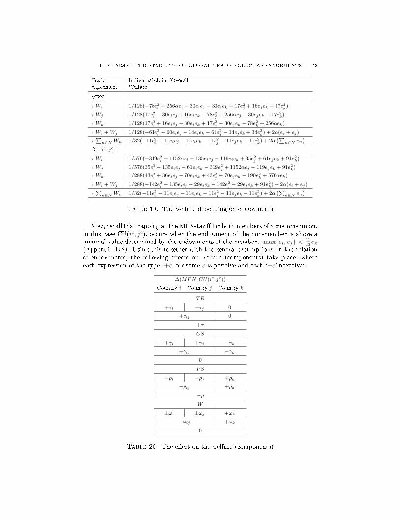
THE FARSIGHTED STABILITY OF GLOBAL TRADE POLICY ARRANGEMENTS 43
Trade Individual/Joint/OverallAgreement Welfare
MFN
�
Wi 1/128(−78e2i + 256αei − 30eiej − 30eiek + 17e2j + 16ejek + 17e2k)
�
Wj 1/128(17e2i − 30eiej + 16eiek − 78e2j + 256αej − 30ejek + 17e2k)
�
Wk 1/128(17e2i + 16eiej − 30eiek + 17e2j − 30ejek − 78e2k + 256αek)
�
Wi +Wj 1/128(−61e2i − 60eiej − 14eiek − 61e2j − 14ejek + 34e2k) + 2α(ei + ej)
�∑n∈N Wn 1/32(−11e2i − 11eiej − 11eiek − 11e2j − 11ejek − 11e2k) + 2α
(∑n∈N en
)CU(ic, jc)
�
Wi 1/576(−319e2i + 1152αei − 135eiej − 119eiek + 35e2j + 61ejek + 91e2k)
�
Wj 1/576(35e2i − 135eiej + 61eiek − 319e2j + 1152αej − 119ejek + 91e2k)
�
Wk 1/288(43e2i + 36eiej − 70eiek + 43e2j − 70ejek − 190e2k + 576αek)
�
Wi +Wj 1/288(−142e2i − 135eiej − 29eiek − 142e2j − 29ejek + 91e2k) + 2α(ei + ej)
�∑n∈N Wn 1/32(−11e2i − 11eiej − 11eiek − 11e2j − 11ejek − 11e2k) + 2α
(∑n∈N en
)Table 19. The welfare depending on endowments
Now, recall that capping at the MFN-tari� for both members of a customs union,in this case CU(ic, jc), occurs when the endowment of the non-member is above aminimal value determined by the endowments of the members, max{ei, ej} < 11
13ek(Appendix B.2). Using this together with the general assumptions on the relationof endowments, the following e�ects on welfare (components) take place, whereeach expression of the type `+c' for some c is positive and each `−c' negative:
∆(MFN,CU(ic, jc))
Country i Country j Country k
TR
+τi +τj 0
+τij 0
+τ
CS
+γi +γj −γk+γij −γk
0
PS
−ρi −ρj +ρk
−ρij +ρk
−ρW
±ωi ±ωj +ωk
−ωij +ωk
0
Table 20. The e�ect on the welfare (components)
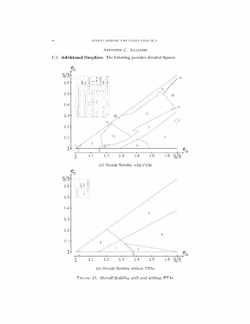
44 STEFAN BERENS AND LASHA CHOCHUA
Appendix C. Analysis
C.1. Additional Graphics. The following provides detailed �gures:
MFN
CU
CUGFT
FTA
FTAHub
FTAGFT
MTA
MTAGFT
1 x x x2 x x x x3 x x x x x x x4 x x x x x x x x5 x6 x x7 x x x8 x x x x x9 x x x x x x
10 x x11 x x x12 x x x x13 x x x x x x14 x x x x x
(a) Overall Stability with PTAs
MFN
MTA
MTAGFT
1 x2 x x3 x4 x
(b) Overall Stability without PTAs
Figure 21. Overall Stability with and without PTAs
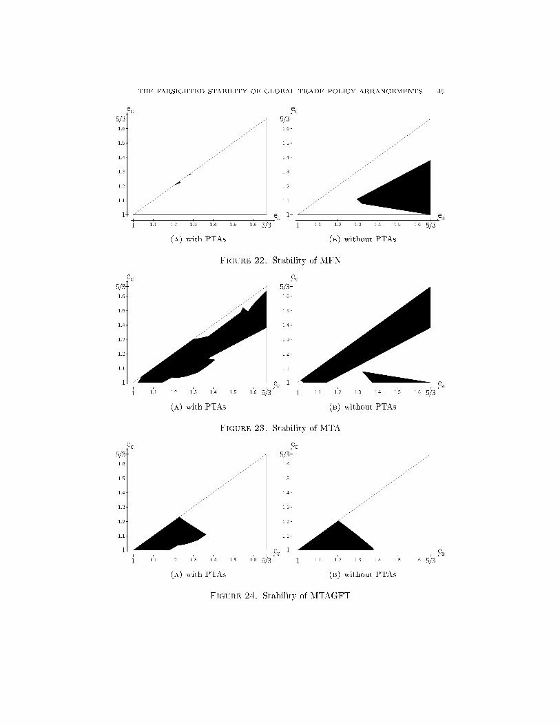
THE FARSIGHTED STABILITY OF GLOBAL TRADE POLICY ARRANGEMENTS 45
(a) with PTAs (b) without PTAs
Figure 22. Stability of MFN
(a) with PTAs (b) without PTAs
Figure 23. Stability of MTA
(a) with PTAs (b) without PTAs
Figure 24. Stability of MTAGFT

46 STEFAN BERENS AND LASHA CHOCHUA
(a) CU (b) CUGFT
Figure 25. Stability of CU
(a) FTA (b) FTAGFT
(c) FTAHub
Figure 26. Stability of FTA
C.2. Exact Intervals. The table here lists the exact intervals where each speci�ctrade agreement is part of the stable set (for the border of the parameter space):

THE FARSIGHTED STABILITY OF GLOBAL TRADE POLICY ARRANGEMENTS 47
Trade Exact
Agreement Interval(s)
eb = emin ≤ ec ≤ emax = ea
CU(b,c) [1.0000000000000000,1.3380093520374081]
CU(c,a) [1.3259853039412157,1.6666666666666667]
FTA(b,c) [1.0000000000000000,1.3807615230460921]
FTA(c,a) [1.3353373413493654,1.6305945223780896]
FTAHub(c)[1.2364729458917836,1.2698730794923179]
[1.3353373413493654,1.3647294589178356]
MTA(c,a) [1.379425517702071,1.635938543754175]
eb = ec = emin ≤ ea ≤ emax
CU(a,b) [1.0240480961923848,1.1108884435537743]
CU(b,c) [1.0240480961923848,1.6666666666666667]
CU(c,a) [1.0240480961923848,1.1108884435537743]
CUGFT [1.0000000000000000,1.1803607214428857]
FTA(a,b) [1.0240480961923848,1.2404809619238477]
FTA(b,c)[1.0240480961923848,1.29124916499666]
[1.483633934535738,1.6666666666666667]
FTA(c,a) [1.0240480961923848,1.2404809619238477]
FTAHub(b) [1.0013360053440215,1.29124916499666]
FTAHub(c) [1.0013360053440215,1.29124916499666]
FTAGFT [1.0000000000000000,1.1803607214428857]
MTA(a,b) [1.0240480961923848,1.1469605878423514]
MTA(c,a) [1.0240480961923848,1.1469605878423514]
MTAGFT [1.0000000000000000,1.1803607214428857]
eb = emin ≤ ea = ec ≤ emax
MFN[1.2044088176352705,1.2297929191716768]
[1.2752171008684035,1.276553106212425]
CU(a,b) [1.0454241816967267,1.2498329993319974]
CU(b,c) [1.0454241816967267,1.2498329993319974]
CU(c,a) [1.0494321977287908,1.6666666666666667]
CUGFT [1.0000000000000000,1.2297929191716768]
FTA(a,b) [1.0494321977287908,1.2925851703406814]
FTA(b,c) [1.0494321977287908,1.2925851703406814]
FTA(c,a) [1.0454241816967267,1.2925851703406814]
FTAHub(a) [1.0454241816967267,1.276553106212425]
FTAHub(b) [1.0454241816967267,1.2925851703406814]
FTAHub(c) [1.0454241816967267,1.276553106212425]
FTAGFT [1.0000000000000000,1.2297929191716768]
MTA(a,b) [1.0494321977287908,1.2244488977955912]
MTA(b,c) [1.0494321977287908,1.2244488977955912]
MTA(c,a) [1.0454241816967267,1.2925851703406814]
MTAGFT [1.0000000000000000,1.2297929191716768]
Table 27. The exact intervals of stability with PTAs

48 STEFAN BERENS AND LASHA CHOCHUA
Trade Exact
Agreement Interval(s)
eb = emin ≤ ec ≤ emax = ea
MFN [1.0000000000000000,1.3780895123580494]
MTA(b,c) [1.0000000000000000,1.0000000000000000]
MTA(c,a) [1.379425517702071,1.6666666666666667]
eb = ec = emin ≤ ea ≤ emax
MFN [1.6666666666666667,1.6666666666666667]
MTA(a,b) [1.0307281229124916,1.1469605878423514]
MTA(b,c)[1.0307281229124916,1.1469605878423514]
[1.3754175016700068,1.6666666666666667]
MTA(c,a) [1.0307281229124916,1.1469605878423514]
MTAGFT [1.0000000000000000,1.3740814963259853]
eb = emin ≤ ea = ec ≤ emax
MTA(a,b) [1.0160320641282565,1.1202404809619237]
MTA(b,c) [1.0160320641282565,1.1202404809619237]
MTA(c,a) [1.0160320641282565,1.6666666666666667]
MTAGFT [1.0000000000000000,1.203072812291249]
Table 28. The exact intervals of stability without PTAs