the application of the genetic algorithm to game theorygga.sourceforge.net/thesis.pdf · ·...

Ludwig-Maximilians-Universitat

Munchen

The Application of the Genetic

Algorithm to Game Theory

Yakov Benilov

Master’s Thesis

March 2006

I would like to thank Professor Martin Schottenloher for the advice and

assistance I received during this thesis; my reviewers Markus and Jelena for

their useful suggestions and corrections; Professor Marks for providing the

life-saving experiment resources; and my parents, for their patience and

encouragement while I wrote this work.

Contents

List of Tables ix

List of Figures xii

List of Program Code xiii

0 Introduction 1

1 The Genetic Algorithm 3

1.1 Introduction . . . . . . . . . . . . . . . . . . . . . . . . . . . . 3

1.1.1 Remarks . . . . . . . . . . . . . . . . . . . . . . . . . . 6

1.2 Genetic Algorithm Specifics . . . . . . . . . . . . . . . . . . . 8

1.3 The Canonical Genetic Algorithm . . . . . . . . . . . . . . . . 10

1.3.1 Formal Definition . . . . . . . . . . . . . . . . . . . . . 11

2 Game Theory Notions 15

2.1 Notes . . . . . . . . . . . . . . . . . . . . . . . . . . . . . . . . 15

2.2 Strategic Games . . . . . . . . . . . . . . . . . . . . . . . . . . 16

2.3 Extensive Games . . . . . . . . . . . . . . . . . . . . . . . . . 19

2.3.1 Extensive Games with Perfect Information . . . . . . . 19

2.3.2 Repeated Games with Perfect Information . . . . . . . 24

2.3.3 Extensive Games with Imperfect Information . . . . . 26

v

vi CONTENTS

3 The Genetic Game Algorithm 31

3.1 Overview . . . . . . . . . . . . . . . . . . . . . . . . . . . . . . 32

3.1.1 Motivations . . . . . . . . . . . . . . . . . . . . . . . . 32

3.1.2 The GGA and the GA . . . . . . . . . . . . . . . . . . 32

3.2 Two GGA Definitions . . . . . . . . . . . . . . . . . . . . . . 33

3.2.1 The GGA for Symmetric Strategic Games . . . . . . . 33

3.2.2 The GGA for Symmetric Repeated Games . . . . . . . 36

3.3 Constraints and Limitations . . . . . . . . . . . . . . . . . . . 37

4 Axelrod’s Evolutionary Experiment 39

4.1 Overview . . . . . . . . . . . . . . . . . . . . . . . . . . . . . . 41

4.1.1 The Game . . . . . . . . . . . . . . . . . . . . . . . . . 41

4.1.2 The Strategy Subset . . . . . . . . . . . . . . . . . . . 42

4.1.3 The Evaluation Functions . . . . . . . . . . . . . . . . 42

4.1.4 The Genetic Functions . . . . . . . . . . . . . . . . . . 45

4.1.5 The Initial Population . . . . . . . . . . . . . . . . . . 46

4.1.6 The Terminating Condition . . . . . . . . . . . . . . . 46

4.2 Detailed Analysis: The Game . . . . . . . . . . . . . . . . . . 46

4.3 Strategies & Evaluation: First Look . . . . . . . . . . . . . . . 47


4.3.2 Encode and Decode . . . . . . . . . . . . . . . . . . . . 48

4.4 Machines And Agents . . . . . . . . . . . . . . . . . . . . . . . 49

4.5 Strategies & Evaluation with Agents . . . . . . . . . . . . . . 54


4.5.2 Encode And Decode . . . . . . . . . . . . . . . . . . . 57

4.6 Fitness, Genetic Functions & The Population . . . . . . . . . 58

4.6.1 Fitness . . . . . . . . . . . . . . . . . . . . . . . . . . . 58

4.6.2 The Genetic Functions . . . . . . . . . . . . . . . . . . 59

4.6.3 The Initial Population . . . . . . . . . . . . . . . . . . 61

CONTENTS vii

4.6.4 The Terminating Condition . . . . . . . . . . . . . . . 61

4.7 Verifying the Definitions . . . . . . . . . . . . . . . . . . . . . 61

4.7.1 Simulation Implementation . . . . . . . . . . . . . . . . 61

4.7.2 Results Comparison . . . . . . . . . . . . . . . . . . . . 62

5 The Contract Game 71

5.1 Background . . . . . . . . . . . . . . . . . . . . . . . . . . . . 72

5.2 The Model . . . . . . . . . . . . . . . . . . . . . . . . . . . . . 73

5.3 Calculating The Subgame Perfect Equilibrium . . . . . . . . . 75

5.3.1 Subgame Perfect Equilibrium . . . . . . . . . . . . . . 75

5.3.2 Back to the Problem . . . . . . . . . . . . . . . . . . . 77

5.4 Applying the GGA . . . . . . . . . . . . . . . . . . . . . . . . 84

5.4.1 The GGA Specification . . . . . . . . . . . . . . . . . . 84

5.4.2 The Strategy Subset and Encoding/Decoding . . . . . 85

5.4.3 The Population . . . . . . . . . . . . . . . . . . . . . . 87

5.4.4 Fitness . . . . . . . . . . . . . . . . . . . . . . . . . . . 87

5.5 Results Analysis . . . . . . . . . . . . . . . . . . . . . . . . . . 88

5.5.1 Results Analysis Under Fitness Version 1 . . . . . . . . 88

5.5.2 Fitness Version 2 . . . . . . . . . . . . . . . . . . . . . 90


5.5.4 Fitness Version 3 . . . . . . . . . . . . . . . . . . . . . 93


5.6 Remarks . . . . . . . . . . . . . . . . . . . . . . . . . . . . . . 95

5.7 Conclusion . . . . . . . . . . . . . . . . . . . . . . . . . . . . . 96

6 Conclusion 97

A Code Listings 99

A.1 The GGA Simulation . . . . . . . . . . . . . . . . . . . . . . . 99

A.1.1 Common Code . . . . . . . . . . . . . . . . . . . . . . 99

viii CONTENTS

A.1.2 Axelrod Simulation . . . . . . . . . . . . . . . . . . . . 101

A.1.3 Contract Game Simulation . . . . . . . . . . . . . . . . 108

A.2 Matlab Programs . . . . . . . . . . . . . . . . . . . . . . . . . 119

B Miscellaneous 123

B.1 History - State Mapping . . . . . . . . . . . . . . . . . . . . . 123

C More on the GGA 125

C.1 Symmetry Partitions . . . . . . . . . . . . . . . . . . . . . . . 126

Bibliography 131

List of Tables

4.1 The Predetermined Strategies Used to Measure Fitness . . . . 43

4.2 Sample Fitness Calculation for strategy w . . . . . . . . . . . 44

4.3 Fitness Calibration . . . . . . . . . . . . . . . . . . . . . . . . 62

4.4 Converting Notations . . . . . . . . . . . . . . . . . . . . . . . 64

4.5 Confirming Results . . . . . . . . . . . . . . . . . . . . . . . . 65

B.1 The Enumeration of History Partitions . . . . . . . . . . . . . 124

ix

x LIST OF TABLES

List of Figures

1.1 The GA flowchart . . . . . . . . . . . . . . . . . . . . . . . . . 9

2.1 Game Definition Dependencies . . . . . . . . . . . . . . . . . . 16

2.2 Extensive Game with Perfect Information Example . . . . . . 21

2.3 Extensive Game Example . . . . . . . . . . . . . . . . . . . . 27

2.4 Rock-Paper-Scissors Payoffs . . . . . . . . . . . . . . . . . . . 29

3.1 The GGA Flowchart . . . . . . . . . . . . . . . . . . . . . . . 34

4.1 The AllC Strategy Machine in the IPD . . . . . . . . . . . . . 50

4.2 The AllD Strategy Machine in the IPD . . . . . . . . . . . . . 51

4.3 The Grim Strategy Machine in the IPD . . . . . . . . . . . . . 51

4.4 The Tit-For-Tat Strategy Machine in the IPD . . . . . . . . . 52

4.5 Calculating the Genes to Watch . . . . . . . . . . . . . . . . . 64

4.6 Simulation Results Using Static Fitness . . . . . . . . . . . . . 65

4.7 A Typical Run from Axelrod’s Dynamic Fitness Experiment . 66

4.8 Dynamic Fitness Results over 50 Generations . . . . . . . . . 68

4.9 Dynamic Fitness Results over 100 Generations . . . . . . . . . 68

5.1 Nash equilibrium efforts x for different bonus rates b . . . . . 83

5.2 Averaged equilibria using 2Tf . . . . . . . . . . . . . . . . . . 91

5.3 Equilibria using 2Tf . . . . . . . . . . . . . . . . . . . . . . . . 92

xi

xii LIST OF FIGURES

5.4 Equilibria using 3Tf . . . . . . . . . . . . . . . . . . . . . . . . 94

A.1 Common Classes and Interfaces . . . . . . . . . . . . . . . . . 100

A.2 The Axelrod Classes . . . . . . . . . . . . . . . . . . . . . . . 102

A.3 The Contract Game Classes . . . . . . . . . . . . . . . . . . . 109

C.1 Modified Rock-Paper-Scissors Payoffs . . . . . . . . . . . . . . 127

List of Program Code

1.1 Genetic Algorithm Pseudo-code . . . . . . . . . . . . . . . . . 10

A.1 The Main Loop of the Simulation . . . . . . . . . . . . . . . . 101

A.2 The Prisoner’s Dilemma Game . . . . . . . . . . . . . . . . . . 101

A.3 Axelrod Static Fitness (Definition 24) . . . . . . . . . . . . . . 105

A.4 Axelrod Dynamic Fitness (Definition 25) . . . . . . . . . . . . 107

A.5 The Contract Game (Definition 28) . . . . . . . . . . . . . . . 108

A.6 1Tf (Equation 5.24) . . . . . . . . . . . . . . . . . . . . . . . . 114

A.7 2Tf (Equation 5.36) . . . . . . . . . . . . . . . . . . . . . . . . 116

A.8 3Tf (Equation 5.39) . . . . . . . . . . . . . . . . . . . . . . . . 117

A.9 The peer-pressure f’n p(b,x) . . . . . . . . . . . . . . . . . . . 119

A.10 The f’n that declares F, p and their 1st and 2nd derivatives . 119

A.11 The f’n that finds the equilibrium x value(s) for a given b . . . 119

A.12 The script that calculates and plots the equilibrium (b,x) pairs 121

xiii

xiv LIST OF PROGRAM CODE

Chapter 0

Introduction

The genetic algorithm (GA) is a powerful computational technique for opti-

misation. The aim of this thesis is to establish a formal language for applying

this technique in the context of strategic game theory, and to illustrate it with

worked examples drawn from real-world game theory problems.

Due to their heuristic nature, the methods outlined here can be used

during the exploratory stages of problem analysis (to get an idea of the

solution landscape, or to find approximate solutions), before the analytical

theory has been developed.

While important work has already been done in the field of GA applica-

tions to game theory, it has been predominantly approached from the eco-

nomic and computer theoretic angle; as a consequence, some of the work

has lacked mathematical rigour. This thesis attempts to formalise some of

the previously developed concepts, using game theoretic language that has

been developed in the previous 15 years, by introducing a genetic algorithm

specifically for games.

The main points of interest in this thesis are a revisit of an important

1987 experiment staged by Robert Axelrod (described in [Axelrod, 1987]),

with the aim of clearing up some of the finer implementation points using

1

2 CHAPTER 0. INTRODUCTION

more formal notation, and an illustration of how the genetic game algorithm

(GGA) may be used to heuristically search for Nash equilibria in extensive

games, using a model called the Contract Game (taken from [Huck et al.,

2003]). Both include experimental analysis, using the simulation that was

created based on the theory in this thesis.

The application of Markov chain theory to the analysis of genetic al-

gorithms has yielded some interesting results concerning convergence. The

research done in this thesis can be extended by further investigation into

the possibility of transferring Markov theory to the genetic algorithms in the

domain of games.

The chapter breakdown is as follows: Chapters 1 and 2 provide intro-

ductions to the genetic algorithm and game theory, respectively. Chapter

3 ties the exposition from Chapters 1 and 2 together by providing several

versions of the GGA. Chapter 4 applies the material from Chapter 3 to Ax-

elrod’s experiment. Chapter 5 focuses on the Contract Game model, first

tackling it analytically and then using the GGA; a comparison of the two ap-

proaches is then made. Chapter 6 is the conclusion. The appendices contain

details about the simulation code for this thesis (Appendix A), and various

miscellaneous information (Appendices B and C).

Chapter 1

The Genetic Algorithm

The purpose of this chapter is to define a vocabulary of terms and concepts

that are necessary for our discussion of genetic algorithms (Section 1.1), to

give a basic introduction to genetic algorithms (Section 1.2), and to illustrate

the presented ideas using one specific algorithm: the Canonical Genetic Al-

gorithm (CGA) (Section 1.3).

1.1 Introduction

A genetic algorithm (GA) is an algorithmic search technique used to find ap-

proximate solutions to optimisation and search problems. The GA’s primary

application is in situations where a multidimensional, non-linear function

needs to be maximised/minimised, and the solution need not be exact, but

rather ”good enough”. Genetic algorithms belong to the class of methods

known as ”weak methods” in the Artificial Intelligence community because

they makes relatively few assumptions about the problem that is being solved

- this makes GAs ideal for ”feeling out” a problem domain and finding solu-

tion candidates, prior to launching into in-depth theoretical analysis.

The GA has three main components, (the first two of) which mimic sim-

3

4 CHAPTER 1. THE GENETIC ALGORITHM

ilar concepts in biological evolution:

1. a sequence of chromosome populations

2. a genetic mechanism which allow a population to be generated from its

predecessor; this mechanism mirrors the main evolutionary processes -

fitness evaluation, selection, recombination and mutation.

3. a terminating condition

We shall now give definitions and explanations of the above terms:

• In this context, a chromosome (or binary string) b = (b1, b2, ..., bm)

of length m is a sequence of m genes. Each gene is a binary number:

bi ∈ 0, 1 ∀i.

• A population of size n is a collection of n chromosomes of equal

length; because a unique chromosome can appear more than once in a

population, we represent it with an n-tuple, rather than a set.

• The genetic mechanism (mentioned earlier) is best thought of as a

stochastic function Ω that transforms one population into another (of

equal size); thus, it is possible for us to define a population sequence

(P (i))i≥0, such that

P (j + 1) = Ω(P (j)) ∀j ≥ 0 (1.1)

The ith population in the population sequence is often referred to as

generation i, or the ith generation. The 0th population (generation

0), commonly called the initial population, is the starting point for

the algorithm and is passed to it as a parameter.

• Encoding/decoding connects points in the problem domain to chro-

mosomes - the initial population may be comprised of encoded points

1.1. INTRODUCTION 5

from the problem domain (for example, if the approximate area of the

fitness maximum is known before the GA is run, the initial population

may be ”seeded” by points from this area), and a chromosome from

the final generation can be decoded back into a problem domain point

when the GA run terminates.

• Fitness evaluation is a process that assigns a quantitative value to

chromosome, based on some metric. That metric may be dynamic

(that is, the fitness of a chromosome relies on what the other chromo-

somes in the population are) or static (the fitness of a chromosome is

independent of the other chromosomes in the population).

• Selection is a process that can be thought of as a gate-keeper - it

regulates which chromosomes from one generation play a part in the

next generation, and which do not. Selection improves the overall pop-

ulation fitness by preventing the propagation of chromosomes with low

fitness values.

• Crossover, or recombination is a process that can create two new

chromosomes (children) from two existing chromosomes (parents); each

child shares genes with both of its parents. Crossover facilitates the

creation of chromosomes that combine the ”best” parts of its parents.

• Mutation is a process that stochastically makes small changes to chro-

mosomes. Mutation helps prevent premature homogeny of a population

and facilitates discovery of previously unvisited optima in the search

space.

• The terminating condition, when satisfied, signals the end of the

GA run - this condition may be chosen to assert whether the best or

average fitness has reached a certain (minimum) level, or perhaps the


condition may be a time constraint (that is, it may assert whether a

generation has been reached or not).

• When we talk about population sequence convergence, we refer

to the situation when a high level of homogeny exists within the pop-

ulation sequence over several generations; this usually implies that the

chromosomes represent a (local or global) maximum of the fitness func-

tion.

The simple description of the GA inner workings is that starting with

an initial population of chromosomes, subsequent generations are created by

putting the previous generation through the genetic mechanisms. The GA

is designed so that both the maximum and average fitness of strategies in

each generation are predominantly increasing1 with time - new populations

continue to be generated until the terminating condition is satisfied.

In a strict interpretation, the genetic algorithm refers to a model intro-

duced and investigated by John Holland [Holland, 1975] and by students of

Holland (e.g. [DeJong, 1975]). It is still the case that most of the exist-

ing theory for genetic algorithms applies either solely or primarily to the

model introduced by Holland, as well as variations on the canonical genetic

algorithm (see Section 1.3.1)2.

1.1.1 Remarks

Unlike some other global search methods, genetic algorithms does not use

gradient information; this also makes their use appropriate in problems in-

volving non-differentiable functions, or functions with multiple local optima.

1The fitness increase is not monotonic - fluctuations on the local time-frame are normal,

but overall growth is generally observed.2[Whitley, 1994]

1.1. INTRODUCTION 7

The fact that GAs make relatively few assumptions about the problem

that is being solved, is an advantage when creating a software implementation

of a GA: time can be saved by using ”off-the-shelf” components, instead

of creating them from scratch - numerous software GA frameworks (which

implement the commonly used mutation, selection and crossover functions)

exist already.

The GA’s generality brings a certain degree of robustness, but the down-

side is that domain-specific methods, where they exist, often out-perform

the GA in terms of computational cost. A common technique is to try to

take the best from both worlds, and to create hybrid algorithms from the

combination of GAs and existing methods.

When adapting the GA to their specific needs, problem solvers need to

make sure that they are performing the correct optimisation - unless an

appropriate choice of fitness function is made, the output of the genetic

algorithm may not be useful to the original problem.

The theory of Markov chains has been demonstrated to be a very power-

ful tool for the theoretical analysis of GAs. There are mainly two approaches

to modeling GAs as Markov chains. The first approach, called population

Markov Chain model, views the sequence of population in GAs as finite

Markov chains on population space( Eiben, Aarts, and Hee (1991), Fogel

(1994), Rudolph (1994)), Leung, Gao and Xu (1997)), while the second ap-

proach models the GAs by identifying the states of the population with prob-

ability vectors over the individual space3 (Reynolds and Gomatam (1996),

Vose (1996)).

3See Section 1.3.1 for explanation of what an individual space is.


1.2 Genetic Algorithm Specifics

An implementation of a genetic algorithm begins with a population of (typ-

ically random) chromosomes. One then evaluates these structures and allo-

cates reproductive opportunities in such a way that those chromosomes which

represent a better solution to the target problem are given more chances to

”reproduce” than those chromosomes which are poorer solutions. The ”good-

ness” of a solution is typically defined with respect to the current population.

It is helpful to view the main execution loop of the genetic algorithm as a

two stage process. It starts with the fitness evaluation of the current popula-

tion. Selection is applied to the current population to create an intermediate

population. Then crossover (recombination) and mutation are applied to

the intermediate population to create the next population. Crossover can

be viewed as creating the next population from the intermediate population.

Crossover is applied to randomly paired chromosomes with a probability de-

noted pc (the population should already be sufficiently shuffled by the random

selection process). Pick a pair of chromosomes. With probability pc ”recom-

bine” these chromosomes to form two new chromosomes that are inserted

into the next population. The process of evaluation, selection, crossover and

mutation forms one generation in the execution of a genetic algorithm.

We can summarise these steps in a flowchart (Figure 1.1).

The pseudo-code representation of the GA can be seen in Listing 1.1.

Usually there are only two main components of most genetic algorithms that

are problem dependent: the problem encoding and the evaluation function.

The remaining components can be reused, and only their parameters (such

as the mutation parameter, crossover parameter, population size) are tuned

to fit the simulation.

As we mentioned earlier, we can divide the fitness metrics into two groups

- dynamic and static. With a static fitness function, the fitness of a chromo-

1.2. GENETIC ALGORITHM SPECIFICS 9

Figure 1.1: The GA flowchart


i=0 // set generation number to zero

i n i t p opu l a t i o n P(0) // initialise a usually random population of individuals

eva luate P(0) // evaluate fitness of all initial individuals of population

while (not done ) do // test for termination condition (time, fitness, etc.)

begin

eva luate P( i ) // evaluate the fitness

i = i + 1 // increase the generation number

s e l e c t P( i ) from P( i −1) // select a sub-population for offspring reproduction

recombine P( i ) // recombine the genes of selected parents

mutate P( i ) // perturb the mated population stochastically

end

Listing 1.1: Genetic Algorithm Pseudo-code

some in a population is independent of the fitness of the other chromosomes

in the same population - the fitness value of a chromosome is absolute. With

a dynamic fitness function, the fitness values are interdependent within a

population - the fitness value of a chromosome is relative. This means that

with a static fitness function, chromosomes from different populations can

be compared and ranked by their fitness values; this is not possible with a

dynamic fitness function, because a chromosome’s fitness only makes sense

in the context of the population that it is in. The type of fitness function

depends on the nature of the landscape being searched by the GA - if the GA

is optimising a variable Examples of both types appear in this thesis: the

original Axelrod experiment in Chapter 4 uses a static fitness function, while

the contract game experiment in Chapter 5 uses a dynamic fitness function.

1.3 The Canonical Genetic Algorithm

We now provide an example of a genetic algorithm: the canonical genetic

algorithm. The CGA defines specific selection, crossover and mutatation

functions, but the fitness, the encoding/decoding functions and the termi-

nating condition all remain problem/simulation specific. Here, we adopt the

1.3. THE CANONICAL GENETIC ALGORITHM 11

more mathematically formal notation that shall be used extensively in later

chapters.

1.3.1 Formal Definition

Taken from Gao [1998]:

We consider the GAs with binary string representations of the encoding

length l and the fixed population size n. The set of chromosomes, or indi-

viduals (encoded feasible solutions) is denoted by B = 0, 1l and is called

the individual space. The set of populations with size n is denoted by Bn.

Particularly, we call B2 = B × B the parents space. The fitness function

f : B → R+0 can be derived from the objective function of the optimization

problem by a certain decoding rule.

With respect to selection in the CGA, the probability that chromosomes

in the current population are copied (i.e., duplicated) and placed in the

intermediate generation is proportion to their fitness. We view the population

as mapping onto a roulette wheel, where each individual is represented by a

space that proportionally corresponds to its fitness. By repeatedly spinning

the roulette wheel, individuals are chosen using ”stochastic sampling with

replacement” to fill the intermediate population.

Definition 1 (Roulette Wheel Selection). The proportional selection op-

erator, GAT fs : Bn → B2, selects a pair of parents from the given population

for reproduction, based on the relative fitness (which is defined by function f)

of the individual in the population. Given the population ~X, the probability

of selecting (Xi, Xj) ∈ B2 as the parents is

PGAT fs ( ~X) = (Xi, Xj) =

f(Xi)∑

X∈ ~X f(X)·

f(Xj)∑

X∈ ~X f(X)(1.2)

with 1 ≤ i ≤ n, 1 ≤ j ≤ n.


For crossover, the CGA uses a technique known as 1-point crossover.

Given two parents, this function generates the first child by first choosing

a random position, and then substituting with the crossover probability pc,

the gene segment after the chosen position in the first parent by the gene

segment after the chosen position in the second parent. The second child is

formed from the left-over segments from the parents. With probability 1−pc,

the children are simply the parents.

Definition 2 (1-point Crossover). For x = (x1, ..., xl) ∈ B, y = (y1, ..., yl) ∈

B, GATc : B2 → B2 is defined as:

P (GATc(x, y) = (x, y)) = 1 − pc (1.3)

P (GATc(x, y) = (zk, wk)) =pc

l∀k = 1, ..., l (1.4)

where zk = (x1, ..., xk, yk+1, ..., yl) and wk = (y1, ..., yk, xk+1, ..., xl).

Example 1 (1-point Crossover). Consider binary chromosomes 1101001100

and yxyyxyxxyy (in the latter, the values 0 and 1 are denoted by x and y).

Using a single randomly chosen recombination point, 1-point crossover occurs

as follows:

11010 \/ 01100

yxyyx /\ yxxyy

Swapping the fragments between the two parents produces the following off-

spring:

11010yxxyy and yxyyx01100

The mutation used in the CGA flips the selected bit (as opposed to gen-

erating a random replacement for it).

1.3. THE CANONICAL GENETIC ALGORITHM 13

Definition 3 (Mutation). The mutation operator, GATm : B → B, oper-

ates on the individual by independently perturbing each gene in a probabilistic

manner and can be specified as follows:

PGATm(X) = Y = p|X−Y |m (1 − pm)1−|X−Y | (1.5)

where pm is the mutation probability.

Finally, we can give the recursive definition of the population sequence in

the CGA.

Definition 4. Based on the genetic operators defined above and a given ini-

tial population ~X(0) of size n, the canonical genetic algorithm (CGA)

can be represented as the following iteration of populations:

~X(k + 1) = T im(T i

c(Tis( ~X(k)))), i = 1, ..., n, k ≥ 0 (1.6)

where (T im, T

is), i = 1, ..., n are independent versions of (GATm, GATs) and

(T 2j−1c , T 2j

c ) =GA T jc , j = 1, ...,

n

2(1.7)

where GAT jc are independent versions of GATc.

Chapter 2

Game Theory Notions

In this chapter, we define, discuss and illustrate game theoretic concepts

that shall be used in consequent chapters. The strategic games section (Sec-

tion 2.2) covers the basic concept of a strategic game, payoff functions and

symmetric games. The extensive games section (Section 2.3) briefly cov-

ers extensive games with both perfect and imperfect information, repeated

games, strategies in such games, and player recall.

2.1 Notes

This chapter is heavy on exposition; the main reason behind this is that

many of the definitions build upon each other, as can be seen in Figure 2.1.

Nonetheless, several ideas have been omitted for simplicity; for example, all

the games involved are pure strategy games (no mixed strategies), and do

not involve chance. There is further explanation as to why mixed strategies

do not feature, in Section 3.3.

Most of the material in this chapter features in [Osborne and Rubinstein,

1994], albeit edited and presented with the narrow focus on what is required

for later on.

15

16 CHAPTER 2. GAME THEORY NOTIONS

Figure 2.1: Game Definition Dependencies

2.2 Strategic Games

Before we launch into the theoretical definitions, we shall introduce probably

the most widely known game, the Prisoner’s Dilemma Game.

Definition 5 (Prisoner’s Dilemma). The Prisoner’s Dilemma (PD) is

a two-player game in which each player has only two pure strategies: co-

operation (C) and defection (D). In any given round, the two players re-

ceive R points if both cooperate and only P points if both defect; a defector

who plays a cooperator gets T points, while the cooperator receives S (with

T > R > P > S and 2R > T + S).

A =

(

R S

T P

)

, B =

(

R T

S P

)

, (2.1)

Example 2.

A =

(

3 0

5 1

)

, B =

(

3 5

0 1

)

, (2.2)

2.2. STRATEGIC GAMES 17

The 2-player game with payoff matrices (A,B) is an example of the Prisoner’s

Dilemma Game, as 5 > 3 > 1 > 0 and 2 × 3 > 5 + 0.

The models we study assume that each decision-maker is ”rational” in

the sense that he is aware of his alternatives, forms expectations about any

unknowns, has clear preferences, and chooses his action deliberately after

some process of optimisation. In the absence of uncertainty, the following

elements constitute a model of rational choice:

• A set A of actions from which the decision-maker makes a choice

• A set C of possible consequences of these actions

• A consequence function g : A→ C that associates a consequence with

each action

• A preference relation (a complete transitive reflexive binary relation)

% on the set C.

Sometimes the decision-maker’s preferences are specified by giving a utility

function U : C → R, which defines a preference relation % by the condition

x % y if and only if U(x) ≥ U(y).

Given any set B ⊆ A of actions that are feasible in some particular case, a

rational decision-maker chooses a feasable action a∗ ∈ B, which is optimal in

the sense that g(a∗) % g(a) for all a ∈ B; alternatively he solves the problem

maxa∈BU(g(a)).

A strategic game is a model of interactive decision-making in which each

decision-maker chooses his plan of action at once and for all, and these choices

are made simultaneously. The model consists of a finite set N of players and,

for each player i, a set Ai of actions and a preference relation on the set of

action profiles (a profile is a collection of values of some variable, one for each

player). We refer to an action profile a = (aj)j∈N as an outcome, and denote

the set ×j∈NAj of outcomes by A.


Notation. For any profile x = (xj)j∈N and any i ∈ N we let x−i be the list

(xj)j∈N\i of elements of the profile x for all players except i.

The formal definition of a strategic game is the following.

Definition 6 (Strategic Game). A strategic game, or normal form

game consists of

1. a finite set N (the set of players)

2. a nonempty set Ai (the set of actions available to player i) for each

player i ∈ N

3. a preference relation %i on A = ×j∈NAj (the preference relation of

player i) for each player i ∈ N

If the set Ai of actions of every player i is finite then the game is finite.

Definition 7 (Payoff Function). Under a wide range of circumstances the

preference relation %i of player i in a strategic game can be represented by

a payoff function ui : A → R (also called a utility function), in the sense

that ui(a) ≥ ui(b) whenever a %i b. We refer to values of such a function

as payoffs (or utilities). Frequently we specify a player’s preference relation

by giving a payoff function that represents it. In such a case we denote the

game by 〈N, (Ai), (ui)〉 rather than 〈N, (Ai), (%i)〉.

Before we illustrate the concept of strategic games with an example, we

would like to introduce a special class of strategic games - symmetric games.

Such games have the property that the participating decision-makers are

not affected by which player ”role” (out of the player set N) they have been

assigned to (for instance, employer-employee games, or incumbent-challenger

games have roles); rather, each player has the same actions available to them,

with the same consequences for a symmetric choice of actions (rock-paper-

scissors is an example of a symmetric game).

2.3. EXTENSIVE GAMES 19

For the moment, we only define symmetry for the simplest type of strate-

gic games - 2-player games.

Definition 8 (Two-player Symmetric Game). Let G = 〈1, 2, (Ai), (%i)〉

be a two-player strategic game; G is called symmetric if it satisfies the

following:

• A1 = A2, and

• (a1, a2) %1 (b1, b2) if and only if (a2, a1) %2 (b2, b1) for all a ∈ A and

b ∈ A.

For H =⟨1, 2, (Ai), (ui)

⟩, the second criterion becomes u1(a1, a2) =

u2(a2, a1) for all a1, a2 ∈ A.

We can now formalise the Prisoner’s Dilemma (from Example 5) using

the definitions that we have introduced.

Example 3 (Prisoner’s Dilemma). Prisoner’s Dilemma is a strategic game

of the form⟨1, 2, (Ai), (%i)

⟩, with:

• A1 = A2 = C,D, and

• (D,C) %1 (C,C) %1 (D,D) %1 (C,D)

• (C,D) %2 (C,C) %2 (D,D) %2 (D,C)

It is trivial to see that it satisfies the symmetry property from Definition 8.

2.3 Extensive Games

2.3.1 Extensive Games with Perfect Information

An extensive game is a detailed description of the sequential structure of the

decision problems encountered by the players in a strategic situation. There is


perfect information in such a game if each player, when making any decision,

is perfectly informed of all the events that have previously occurred. We

initially restrict attention to games in which no two players make decisions

at the same time and all relevant moves are made by players (no randomness

ever intervenes) - the first restriction is removed later on.

Definition 9 (Extensive Game with Perfect Information). An extensive

game with perfect information has the following components.

1. A set N (the set of players)

2. A set H of sequences (finite or infinite) that satisfies the following three

properties.

• The empty sequence ∅ is a member of H.

• If (ak)k=1,...,K ∈ H (where K may be infinite) and L < K then

(ak)k=1,...,L ∈ H.

• If an infinite sequence (ak)∞k=1 satisfies (ak)k=1,...,L ∈ H for every

positive integer L then (ak)∞k=1 ∈ H.

(Each member of H is a history; each component of a history is an

action taken by a player.) A history (ak)k=1,...,K ∈ H is terminal if

it is infinite or if there is no aK+1 such that (ak)k=1,...,K+1 ∈ H. The

set of terminal histories is denoted Z.

3. A function P that assigns to each nonterminal history (each member

of H \Z) a member of N . (P is the player function, P (h) being the

player who takes an action after the history h.)

4. A preference relation %i on Z (the preference relation of player i)

for each player i ∈ N .


We interpret such a game as follows. After any nonterminal history h

player P (h) chooses an action from the set

A(h) = a : (h, a) ∈ H

(here, if h is a history of length k, (h, a) denotes the history of length k + 1

consisting of h followed by a). The empty history is the starting point of the

game; it is referred to as the initial history. At this point player P (∅) chooses

a member of A(∅). For each possible choice a0 from this set player P (a0)

subsequently chooses a member of the set A(a0); this choice determines the

next player to move, and so on. A history after which no more choices have

to be made is terminal. Note that a history may be an infinite sequence of

actions.

Here is an example, illustrating the above definition.

Figure 2.2: Extensive Game with Perfect Information Example

Example 4 (Extensive Game with Perfect Information). Two people use the

following procedure to share two desirable identical indivisible objects. One

of them proposes an allocation, which the other then either accepts or rejects.

In the event of rejection, neither person receives either of the objects. Each

person cares only about the number of objects he obtains.


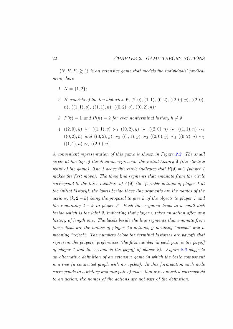
〈N,H, P, (%i)〉 is an extensive game that models the individuals’ predica-

ment; here

1. N = 1, 2;

2. H consists of the ten histories: ∅, (2, 0), (1, 1), (0, 2), ((2, 0), y), ((2, 0),

n), ((1, 1), y), ((1, 1), n), ((0, 2), y), ((0, 2), n);

3. P (∅) = 1 and P (h) = 2 for ever nonterminal history h 6= ∅

4. ((2, 0), y) ≻1 ((1, 1), y) ≻1 ((0, 2), y) ∼1 ((2, 0), n) ∼1 ((1, 1), n) ∼1

((0, 2), n) and ((0, 2), y) ≻2 ((1, 1), y) ≻2 ((2, 0), y) ∼2 ((0, 2), n) ∼2

((1, 1), n) ∼2 ((2, 0), n)

A convenient representation of this game is shown in Figure 2.2. The small

circle at the top of the diagram represents the initial history ∅ (the starting

point of the game). The 1 above this circle indicates that P (∅) = 1 (player 1

makes the first move). The three line segments that emanate from the circle

correspond to the three members of A(∅) (the possible actions of player 1 at

the initial history); the labels beside these line segments are the names of the

actions, (k, 2 − k) being the proposal to give k of the objects to player 1 and

the remaining 2 − k to player 2. Each line segment leads to a small disk

beside which is the label 2, indicating that player 2 takes an action after any

history of length one. The labels beside the line segments that emanate from

these disks are the names of player 2’s actions, y meaning ”accept” and n

meaning ”reject”. The numbers below the terminal histories are payoffs that

represent the players’ preferences (the first number in each pair is the payoff

of player 1 and the second is the payoff of player 2). Figure 2.2 suggests

an alternative definition of an extensive game in which the basic component

is a tree (a connected graph with no cycles). In this formulation each node

corresponds to a history and any pair of nodes that are connected corresponds

to an action; the names of the actions are not part of the definition.


Player Strategy

A strategy of a player in an extensive game is a plan that specifies the action

chosen by the player for every history after which it is his turn to move, even

for histories that, if the strategy is followed, are never reached.

Definition 10 (Player Strategy in an Extensive Game with Perfect Infor-

mation). A strategy of player i ∈ N in an extensive game with perfect

information 〈N,H, P, (%i)〉 is a function that assigns an action in A(h) to

each nonterminal history h ∈ H \ Z for which P (h) = i.

Example 5 (Player Strategy in an Extensive Game with Perfect Informa-

tion). Consider the game from Example 4 (that is displayed in Figure 2.2).

Player 1 takes an action only after the initial history ∅, so that we can iden-

tify each of her strategies with one of three possible actions that she can take

after this history: (2, 0), (1, 1) and (0, 2). Player 2 takes an action after

each of the three histories (2, 0), (1, 1) and (0, 2), and in each case has two

possible actions. Thus we can identify each of his strategies as a triple a2b2c2

where a2, b2 and c2 are the actions that he chooses after the histories (2, 0),

(1, 1) and (0, 2). The interpretation of player 2’s strategy a2b2c2 is that it is

a contingency plan: if player 1 chooses (2, 0) then player 2 will choose a2; if

player 1 chooses (1, 1) then player 2 will choose b2; and if player 1 chooses

(0, 2) then player 2 will choose c2.

Simultaneous Moves

To model situations in which players move simultaneously after certain his-

tories, each of them being fully informed of all past events when making his

choice, we can modify the definition an extensive game with perfect informa-

tion (Definition 9) as follows.


Definition 11 (Extensive Game with Perfect Information and Simultaneous

Moves). An extensive game with perfect information and simulta-

neous moves is a tuple 〈N,H, P, (%i)〉 where N , H, %i for each i ∈ N are

the same as in Definition 9, P is a function that assigns to each nontermi-

nal history a set of players, and H and P jointly satisfy the condition that

for every nonterminal history h there is a collection Ai(h)i∈P (h) of sets for

which A(h) = a : (h, a) ∈ H = ×i∈P (h)Ai(h).

A history in such a game is a sequence of vectors; the components of each

vector ak are the actions taken by the players whose turn it is to move after

the history (al)k−1l=1 . The set of actions among which each player i ∈ P (h) can

choose after the history h is Ai(h); the interpretation is that the choices of

the players in P (h) are made simultaneously. A strategy of player i ∈ N in

such a game is a function that assigns an action in Ai(h) to every nonterminal

history h for which i ∈ P (h).

2.3.2 Repeated Games with Perfect Information

The model of a repeated game captures the situation in which players re-

peatedly engage in a strategic game G, which we refer to as the constituent

game. We restrict attention to games in which the action set of each player

is compact and the preference relation of each player is continuous (a pref-

erence relation % on A is continuous if a % b whenever there are sequences

(ak)k and (bk)k in A that converge to a and b respectively for which ak % bk

for all k). On each occasion that G is played, the players choose their actions

simultaneously. When taking an action, a player knows the actions previ-

ously chosen by all players. We model this situation as an extensive game

with perfect information and simultaneous moves, as follows.

Definition 12 (Infinitely Repeated Game with Perfect Information). Let

G = 〈N, (Ai), (%i)〉 be a strategic game; let A = ×i∈NAi. An infinitely


repeated game with perfect information of G is an extensive game

with perfect information and simultaneous moves⟨N,H, P, (%∗

i )⟩

in which

1. H = ∅ ∪ (∪∞t=1A

t)∪A∞ (where ∅ is the initial history and A∞ is the

set of infinite sequences (at)∞t=1 of action profiles in G)

2. P (h) = N for each nonterminal history h ∈ H

3. %∗i is a preference relation on A∞ that extends the preference relation %i

in the sense that it satisfies the following condition of weak separability:

if (at) ∈ A∞, a ∈ A, a′ ∈ A and a %i a′ then

(a1, ..., at−1, a, at+1, ...) %∗i (a1, ..., at−1, a′, at+1, ...)

for all values of t.

We now introduce the concept of a finitely repeated game. The formal

description of a finitely repeated game is very similar to that of an infinitely

repeated game.

Definition 13 (T-period Repeated Game with Perfect Information). For

any positive integer T a T -period finitely repeated game with perfect

information of the strategic game 〈N, (Ai), (%i)〉 is an extensive game with

perfect information that satisfies the conditions in Definition 12 when the

symbol ∞ is replaced by T . We restrict attention to the case in which the

preference relation %∗i of each player i in the finitely repeated game is rep-

resented by the function∑T

t=0 ui(at)/T , where ui is a payoff function that

represents i’s preference in the constituent game.

Definition 14 (Canonical Iterated Prisoner’s Dilemma). The canonical ver-

sion of the Iterated Prisoner’s Dilemma (IPD) is a T-period repeated game

with perfect information, with the Prisoner’s Dilemma (Definition 3) as its

constituent game.


2.3.3 Extensive Games with Imperfect Information

In each of the models we have introduced previously, the players are not

perfectly informed, in some way, when making their choices. In a strategic

game a player, when taking an action, does not know the actions that the

other players take. In an extensive game with perfect information, a player

does not know the future moves planned by the other players. The model

that we define here - an extensive game with imperfect information - differs

in that the players may in addition be imperfectly informed about some (or

all) of the choices that have already been made.

The following definition generalises that of an extensive game with perfect

information (Definition 9) to allow players to be imperfectly informed about

past events when taking actions. It does not incorporate the generalisation

in which more than one player may move after any history (Definition 11),

nor does it allow for exogenous uncertainty: moves may not be made by

”chance”. The latter is not incorporated in our definition not as a result of

any incompatibilities in the concepts, but purely for simplicity’s sake; we will

not require it for the examples and analyses that come later.

Definition 15 (Extensive Game). An extensive game is a tuple⟨N,H,

P,(Ii), (%i)⟩

where N , H, %i for each i ∈ N are the same as in Definition

9, and a partition Ii of h ∈ H : P (h) = i for each player i ∈ N with the

property that A(h) = A(h′) whenever h and h′ are in the same member of

the partition. For Ii ∈ Ii we denote by A(Ii) the set A(h) and by P (Ii) the

player P (h) for any h ∈ Ii. (Ii is the information partition of player i;

a set Ii ∈ Ii is an information set of player i.)

We interpret the histories in any given member of Ii to be indistinguish-

able to player i. Thus the game models a situation in which after any history

h ∈ Ii ∈ Ii player i is informed that some history in Ii has occured but is

not infomed that the history h has occured. The condition A(h) = A(h′)


whenever h and h′ are in the same member of Ii captures the idea that if

A(h) 6= A(h′) then player i could deduce, when he faced A(h), that the

history was not h′, contrary to our interpretation of Ii.

If 〈N,H, P, (Ii)i∈N , (%i)i∈N〉 is an extensive game (as in Definition 15)

and every member of the information partition of every player is a singleton,

then 〈N,H, P, (%i)i∈N〉 is an extensive game with perfect information (as in

Definition 9).

Figure 2.3: Extensive Game Example

Example 6 (Extensive Game). An example of an extensive game with im-

perfect information is shown in Figure 2.3. In this game player 1 makes the

first move, choosing between L and R. If she chooses R, the game ends. If

she chooses L, it is player 2’s turn to move; he is informed that player 2

chose L and chooses A or B. In either case it is player 1’s turn to move,

and when doing so she is not informed whether player 2 chose A or B, a fact

indicated in the figure by the dotted line connecting the ends of the histories

after which player 1 has to move for the second time, choosing an action from


the set l, r. Formally, we have P (∅) = P (L,A) = P (L,B) = 1, P (L) = 2,

I1 = ∅, (L,A), (L,B), and I2 = L (player 1 has two information

sets and player 2 has one). The numbers under the terminal histories are

players’ payoffs. (The first number in each pair is the payoff of player 1 and

the second is the payoff of player 2.)

In Definition 15, we do not allow more than one player to move after any

history. However, there is a sense in which an extensive game as we have

defined it can model such a situation. To see this, consider Example 6 above.

After player 1 chooses L, the situation in which players 1 and 2 are involved

is essentially the same as that captured by a game with perfect information

in which they choose actions simultaneously. (This is the reason that in much

of the literature the definition of an extensive game with perfect information

does not include the possibility of simultaneous moves.) With this in mind,

we can see that we need only trivial (if technically messy) adjustments, in

order to represent the games from Definitions 12 and 13 as extensive games

with imperfect information.

Before we introduce a specific type of repeated game with imperfect in-

formation (Definition 17), we extend the concept of symmetry that was first

introduced in the 2-player symmetric games definition (Definition 8).

Definition 16 (m-player Symmetric Strategic Game). An m-player strategic

game⟨N, (Ai), (ui)

⟩(where |N | = m) is symmetric if the following condi-

tions hold:

1. Every player has the same action space: A = A1 = A2 = ... = Am.

2. Every player has a symmetric payoff function in the following sense:

pick two action profiles a, a′ ∈ A and a pair of players i, j ∈ N arbi-

trarily. If ai = a′j and a−i can be obtained from a′−j by a permutation

of actions, then ui(a) = uj(a′).


We illustrate the definition with an example.

Example 7 (m-player Symmetric Strategic Game). A 3-player Rock-Paper-

Scissors game 〈1, 2, 3, R,P, S, (ui)〉 has the following rules:

• a starting pot of winnings is split between 3 players at the end of each

game

• if players pick one of each strategy, or everyone picks the same strategy,

then the pot is shared equally

• if one player’s strategy beats the others’ strategies, she wins the pot

• if two players’ strategies are the same and beat the third’s, then they

share the pot

This game is symmetric if the payoff profiles are as in Figure 2.4 (tuples

correspond to payoffs for players (I,II,III)).

Figure 2.4: Rock-Paper-Scissors Payoffs

Definition 17 (m-Player Symmetric T-period Repeated Game). Let the con-

stituent game G = 〈N, (Ai), (%i)〉 be an m-player symmetric strategic game;


let A = ×i∈NAi. A T-period repeated game of G is an extensive game

〈N,H, P, (Ii), (%i)〉 in which

1. H = ∅ ∪ (∪Tt=1A

t) (where ∅ is the initial history and AT is the set of

T-length sequences (at)Tt=1 of action profiles in G)

2. P (h) = N for each nonterminal history h ∈ H

3. the preference relation %∗i of each player i is represented by the func-

tion∑T

t=0 ui(at)/T , where ui is a payoff function that represents i’s

preference in the constituent game.

4. Ii = Ij for all i, j ∈ N

A player’s strategy in an extensive game with perfect information is a

function that specifies an action for every history after which the player

chooses an action (Definition 10). The following definition is an extension to

a general extensive game.

Definition 18 (Player Strategy in an Extensive Game). A strategy of

player i ∈ N in an extensive game 〈N,H, P, (Ii), (%i)〉 is a function that

assigns an action in A(Ii) to each information set Ii ∈ Ii.

Chapter 3

The Genetic Game Algorithm

In Chapter 1, we discussed the concept of the genetic algorithm in broad

terms. In this chapter, the goal is to find a meaningful way to apply the

genetic algorithm to problems in game theory. To that end, we shall take

various definitions that we introduced in Chapter 2 and combine them with

the ideas from Chapter 1; our results will be several formal definitions (cov-

ering the different flavours of games) that we will call the Genetic Game

Algorithm1 (GGA).

After an discussion of the motivations behind the GGA and how it differs

from the GA (Section 3.1), we shall define two versions of the GGA - one for

symmetric strategic games (Section 3.2.1), and one for 2-player symmetric

repeated games (Section 3.2.2). Constraints and limitations of the given

algorithms are discussed in Section 3.3, and more general versions of the

GGA can be found in Appendix C.

To the author’s best knowledge, almost all of the material in this chapter

(at least in its present form), is original.

1This name should be interpreted as ”Genetic Algorithm for Games”, rather than an

”Algorithm for Genetic Games”.

31

32 CHAPTER 3. THE GENETIC GAME ALGORITHM

3.1 Overview

3.1.1 Motivations

The main motivation for the GGA stems from the desire to have an algorith-

mic method for finding the best strategy in a given action/strategy space,

just as the GA is an algorithmic method for finding the best individual in a

given population space. Another goal of the GGA is to formalise some of the

prior economic and game theoretic experimental work on strategy evolution.

For me personally, there were numerous times when the understanding of an

interesting experiment was hindered by the imprecise language used in its

exposition. By providing some precise but flexible definitions (built on the

very strict game theoretic definitions and results that has been developed

over the last 15 years), an attempt is made to alleviate these issues. Another

benefit of formalisation is that for any experiments that utilise the GGA, the

simulation implementation time is reduced (this is because a mathematically

stipulated model is the most precise specification that a software implementer

can hope for, meaning the written software can be written quicker and with

fewer bugs).

Beside strategy evolution, the GGA can be applied to other situations

involving discrete population, discrete-time dynamics, such as experiments

investigating population convergence or equilibrium points.

3.1.2 The GGA and the GA

In Chapter 1, we formalised only those parts of the GA that were domain

and problem independent, and even then, not all of them (for instance, we

introduced the concept of a terminating condition, which is but we did not

formally define it). As we are focusing on a specific domain of games - which

comes with its own formal language and structure - we can now precise in

3.2. TWO GGA DEFINITIONS 33

our definitions.

The GGA is different to the GA in that the evaluation process (from the

GA) is broken down into fitness, encoding and decoding in the GGA, which

are collectively called the evaluation functions; the GGA flowchart (Figure

3.1) reflects this decomposition. The most important one of all, the fitness

function, is (the only place in the GGA) where games are played. While

we can now specify the domains of the evaluation functions, they are in fact

problem-specific - we shall see several examples of these when we analyse

problems in the next two chapters.

3.2 Two GGA Definitions

Two versions of the GGA are presented in this chapter: Definition 19 (for

m-player symmetric strategic games) and Definition 20 (for a 2-player sym-

metric T-period repeated games). More general versions of the GGA can be

found in Appendix C - since they are not necessary for use in later chapters,

and are not different enough conceptually to warrant extra attention, we do

not present them here.

3.2.1 The GGA for Symmetric Strategic Games

Before we introduce the simplest version of the GGA, we need to define some

notation:

Notation. Wherever a function of the form Tz : X → Y has been defined,

Tz,k will always be understood to be

Tz,k : Xk → Y k, (x1, x2, ..., xk) 7→ (Tz(x1), Tz(x2), ..., Tz(xk)) (3.1)

for x1, ..., xk ∈ X.

Notation. R+0 refers to the set x ∈ R|x ≥ 0


Figure 3.1: The GGA Flowchart

3.2. TWO GGA DEFINITIONS 35

Definition 19 (The Genetic Game Algorithm for an m-player Symmetric

Strategic Game). The GGA for an m-player symmetric game G =⟨N, (Ai),

(ui)⟩

consists of:

1. a set D ⊆ A(= A1 = A2), the action subset, containing 2k elements

(for some k ∈ N),

2. the evaluation functions:

• Te : D → B (an invertible encode function),

• Td : B → D (the inverse of encode, the decode function),

• Tf : Dn → (R+0 )n (fitness)

where B = 0, 1k (k is as in point 1),

3. the genetic functions:

• (T is)

n/2i=1 : Bn × (R+

0 )n → B2 (selection) - its inputs are the current

population and the population’s fitness,

• (T ic)

n/2i=1 : B2 → B2 (crossover) - its inputs are two parent chromo-

somes,

• Tm : B → B (mutation) - its input is the chromosome undergoing

mutation

4. the terminating condition function Tt : Bn × N → true, false - its

input is a population and its generation number,

5. an n-tuple of actions, ~Y ∈ Dn (with n a multiple of 2), called the initial

population,


Then the population sequence ( ~X(p))p∈0,1,2,...,c, ~X(p) ∈ Bn is obtained

using the following:

~X(p) =

Te,n(~Y ) for p = 0

(p1, p2, ..., pn) for 1 ≤ p ≤ c(3.2)

where ∀i = 1, ..., n2,

(p2i−1, p2i) = Tm,2(Tic(T

is( ~X(p− 1), Tf (Td,n( ~X(p− 1)))))) (3.3)

In the above expressions, the terminating generation c ∈ N is a number

that satisfies the following conditions:

0 ≤ j < c⇒ Tt( ~X(j), j) = false , and (3.4)

Tt( ~X(c), c) = true. (3.5)

Remark 1. For a game G =⟨N,A, (ui)

⟩and action subset D ⊆ A (G and

D as in Definition 19), the action subset induces a game G′ =⟨N, D, (ui)

⟩.

This means that G′, not G, is the game in which the GGA is searching for

the best action. Thus, it is imperative that D approximates A as closely as

possible, otherwise the optimum solution from D may not be a close enough

approximation of the optimum solution from A.

The GGA from Definition 19 is used in the analysis of the Contract Game

problem from Chapter 5.

3.2.2 The GGA for Symmetric Repeated Games

The major difference between the GGA for extensive games and the GGA

for strategic games, in that the ”individuals” encoded in the chromosomes

are strategies, rather than actions.

As before, only one (narrow) extensive game GGA version is given here;

this is done so that we can maintain our focus and move forward to our

examples. Again, more general versions are provided in the Appendix.

3.3. CONSTRAINTS AND LIMITATIONS 37

Definition 20 (The Genetic Game Algorithm for an m-player Symmet-

ric T-period Repeated Game). The GGA for an T-period repeated game

G =⟨N,H, P, (Ii), (%i)

⟩(see Definition 17) with an m-player symmetric

constituent game 〈N, (Ai), (ui)〉, is defined in exactly the same way as in De-

finition 19, except that instead of instead of D, we have W , subset of player

strategies for the game G, (strategies are as defined in Definition 18), with

W containing 2k elements (for some k ∈ N).

Remark 2. The argument here is similar to the one made in Remark 1: the

GGA is trying to find the ”best” strategy from the strategy subset W , not from

the set of all strategies for the game; thus, for the GGA search to be useful,

we need to pick W so that the strategies within have enough complexity to be

useful in the problem being solved.

The GGA from Definition 20 is used in the analysis of the Axelrod ex-

periment from Chapter 4.

3.3 Constraints and Limitations

There are certain limitations regarding which games can be fitted to the

GGA:

1. The cardinality of the action/strategy subset must be power of 2.

If the cardinality is not a power of 2, then there will exist chromosomes

which do not correspond to any action/strategy - this would mean that

the mutation and crossover operators are not closed.

2. The number of individuals in each of the populations (in the population

sequence) must be a multiple of 2.

This restriction is in place only for the sake of notation simplicity in

the crossover operator, which tends to be symmetric. In practice, large

populations are usually used and this restriction becomes a non-issue.


3. The GGA cannot model dynamics that feature non-integer populations,

such as replicator dynamics.

This incompatibility is not of crucial importantance, as continuous pop-

ulation dynamics have already been the focus of much in-depth re-

search, yielding results that eclipse anything presented here regarding

discrete population models ([Weibull, 1995] is a great resource on this

topic).

Chapter 4

Axelrod’s Evolutionary

Experiment

In 1979, Robert Axelrod (University of Michigan) hosted a tournament to see

what kinds of strategies would perform best over the long haul in the Iterated

Prisoner’s Dilemma (IPD) game. The fourteen entries (plus the ”random”

strategy entered by Axelrod himself) - all computerized IPD strategies - were

submitted not just by game theorists, but also by economists, biologists, com-

puter scientists and psychologists. The tournament pitted the entries against

each other in a round-robin format (that is, each contestant is matched in

turn against every other contestant), with 200 rounds of PD played during

each ”match”, and was run five times to smooth out random effects. Tit-For-

Tat (TFT), the winning strategy (that is, the one that averaged the highest

score overall), entered by Anatol Rapoport (a mathematical psychologist),

was the simplest of all submitted strategies, with just two rules:

1. in the first round, cooperate

2. in each subsequent round, play the opponent’s action from the previous

round

39

40 CHAPTER 4. AXELROD’S EVOLUTIONARY EXPERIMENT

Axelrod staged a secound tournament, and had sixty-two entry submis-

sions from 6 countries (plus the ”random” strategy, as before). The rules

were only slightly modified from the first tournament: games were now of a

random length with median 200, rather than exactly 200 rounds; this avoided

the complications from programs having special cheating rules for the last

game. Surprisingly, given that every submitter had full information about

the structure and results of the first tournament, Tit-For-Tat once again

emerged as the winner.

After his tournaments, Axelrod went on to stage several ”evolutionary”

tournaments (or rather experiments, since these did not involve submitted

strategies). These experiments modelled the players in the IPD game as

stimulus-response automata - the stimulus was the state of the game, defined

as both players’ actions over the previous several moves, and the response was

the next period’s action (or actions) - and investigated the question of what

the best-performing IPD automaton strategy is. The focus of this chapter

will be on the specific experiment presented in [Axelrod, 1987] (and revisited

in [Marks, 1989]) - we shall describe the experimental setup as a GAA.

This is done with two aims in mind: to illustrate the GGA and at the

same time, to try to improve on one of the weaker aspects of Axelrod’s

unquestionably important and influential work - its mathematically loose

style of exposition. This perceived weakness should not be interpreted as

a challenge to the rigour or the correctness of the experiment itself. For

me personally, as I studied the aforementioned papers on this experiment,

the informal approach at times hindered my understanding of the material;

consequently, this chapter is designed to serve as a companion to Axelrod’s

and Marks’ research, by clarifying some of the murkier points and ”colouring

in” the sketches that they lay out.

We shall start with an overview in Section 4.1, which is roughly broken

down into the the following parts, mirroring Definition 20: the game, the

4.1. OVERVIEW 41

strategy subset available to players, the evaluation functions, the genetic

functions, and the initial population. Then we proceed to formally describe

the experiment in detail in Sections 4.2, 4.3, 4.4, 4.5 and 4.6, using the defin-

itions from the previous chapters. In Section 4.7, we discuss the simulations

that we built to test our definitions, and the experiments that we ran on

them.

4.1 Overview

We are going to describe Axelrod’s experimental setup as a GGA, specifically

the version from Definition 20.

4.1.1 The Game

The game that the experiment revolves around is the Iterated Prisoner’s

Dilemma (which is a T-period repeated game with the Prisoner’s Dilemma as

the constituent game). What needs to be decided is whether we should model

the situation with the canonical, perfect information version (Definition 14),

or its imperfect information equivalent.

Unlike the tournament that we analyse in this chapter (which involves

stimulus-response automata), Axelrod’s first tournament pitted programmed

strategy subroutines against each other; although the extensive game being

played was not explicitly defined in Axelrod’s paper, one fact about his sub-

routines - that they were allowed to have persistent local variables - helped

determine what that definition should be.

In simple terms, persistent local variables allow the subroutines to ”re-

member” between the rounds of the repeated game; hence, a strategy sub-

routine can choose to remember every move that it and its opponent made.

The implication stemming from this fact, is that the most appropriate game


for our model is the repeated game with perfect information (that is, there

is an information set for each history in the game).

4.1.2 The Strategy Subset

The strategy subset, being explored in this experiment, contains all strategies

which have:

• an action for every possible combination of moves over the previous 3

rounds of the game; each player makes one of two moves - cooperate

or defect - at each of the 3 rounds, which brings it to 26 = 64 possible

combinations, and hence, 64 actions. The strategy’s current action is

determined solely by what happened in the previous 3 rounds.

• a ”fake” history (or ”false memory”), which is used by the strategy only

in the first 3 rounds, when there isn’t enough real history to determine

an action.

4.1.3 The Evaluation Functions

The binary representation of the strategy described above is quite straight-

forward; since the Prisoner’s Dilemma is a symmetric game with only two

possible actions, we can simply represent ”cooperate” as 0, and ”defect” as

1. Overall, each strategy is represented in the chromosome space by a 70 bit

chromosome. The first 6 bits store the fake history, and the remaining bits

store instructions regarding which action to take for each of the 64 possible

histories over the previous 3 rounds.

1 2 3 4 5 6︸︷︷︸

phantom history

7 8 9 ... 68 69 70︸︷︷︸

behaviour rules

4.1. OVERVIEW 43

Strategy In Axelrod Name Author(s)

v1 K60R TFT with Check J.Graaskamp & K.Katzen

for Random

v2 K91R Revised State J.Pinckley

Transition

v3 K40R Discoverer R.Adams

v4 K67R Tranquilizer C.Feathers

v5 K76R Tester D.Gladstein

v6 K77R Adjuster S.Feld

v7 K85R Slow-Never R.Falk & J.Langsted

v8 K47R Fink R.Hufford

Table 4.1: The Predetermined Strategies Used to Measure Fitness

Fitness

In his 1984 report, Axelrod specified a set (let us call it T8) of eight strategies

from his second tournament (that are listed in Table 4.1); the T8 strategies

could be used as representatives of the complete set of 63 strategies entered

in the tournament. Using the following equation:

f(w) = c0+8∑

i=1

ckwk

= 110.55 + (0.1574) w2 + (0.1506) w1 + (0.1185) w3

+ (0.0876) w4+ (0.0579) w6 + (0.0492) w7

+ (0.0487) w5+ (0.0463) w8

where wi is the score strategy w gets playing 151 rounds of the IPD against

vi, Axelrod reported that the estimates correlated with the actual tourna-

ment scores at a variance of 0.98 (so 98% of the variance in his tournament

scores is explained by knowing a strategys performance against the T8). Con-


sequently, Axelrod defines the evolutionary experiment’s population fitness

using the above equation (an example fitness calculation can be seen in Table

4.2).

Opponent Outcome after 151 Rounds wk ckwk

v1 STRRPTS...R 420 63.252

v2 RRRRRRR...R 453 71.3022...

......

...

v8 · · · · · · · · ·∑8

i=1 ckwk 271.05

f(w): c0 +∑8

i=1 ckwk 381.60

Table 4.2: Sample Fitness Calculation for strategy w

(R, S, T, and P refer to the four possible outcomes of the Prisoner’s

Dilemma, as defined in Definition 5.)

This static1 fitness measure was engineered with two assumptions in mind:

1. The 8 IPD strategies that it features provide an accurate approximation

of the 63 strategies entered into Axelrod’s second tournament

2. Those 63 strategies are representative of the entire population of IPD

strategies, and performance against these 63 strategies provides an ac-

curate approximation of performance against all IPD strategies.

If these assumptions did not hold, it could mean that the optimal strategy,

found using the static fitness, would be suboptimal with respect to the entire

set of all IPD strategies. In fact, [Nachbar, 1988] challenges the second

assumption, arguing that the results from Axelrod’s second tournament are

tainted by the entrants’ prior knowledge of the results of the first tournament,

which may have been suboptimal.

1See discussion in Section 1.2.

4.1. OVERVIEW 45

Axelrod was aware of such doubts, because he introduces an alternative

fitness function, one that it no longer relies on these assumptions. During

fitness calculation for a strategy, the function pits that strategy against every

other in the population (including itself) in an IPD game, and averages the

outcome - it is a dynamic fitness function.

4.1.4 The Genetic Functions

Selection

The technique used here for selecting chromosomes (for crossover and muta-

tion) is called ”sigma scaling”. First, the mean and the standard deviation

(SD) of the fitness values is calculated before the selection; strategies with

fitness less than one SD lower than the mean are discarded (that is, they

play no part in forming the next generation), strategies with fitness over on

SD higher than the mean are selected twice, and the remaining strategies are

each selected only once.

Crossover

The standard one-point crossover technique (as in the CGA - see Definition 2)

is used: a gene position on the parent chromosomes is (uniformly) randomly

selected; then with the crossover probability pc, the children are created from

both parent chromosomes being sliced at that point and their tail segments

switched, or with probability 1 − pc the children chromosomes are simply

clones of the parent chromosomes.

Mutation

The CGA mutation technique (see Definition 3) is used: each gene is per-

turbed in a probabilistic manner.


4.1.5 The Initial Population

The initial population is drawn randomly, so each chromosome is generated

through 70 Bernoulli(12) trials.

4.1.6 The Terminating Condition

The terminating condition is a trigger condition that interrupts the GGA at

the 50th generation.

4.2 Detailed Analysis: The Game

As discussed in Section 4.1.1, the game being played is the Canonical IPD

from Definition 14 (which is a T-period repeated game with perfect informa-

tion, with the Prisoner’s Dilemma as the constituent game), with T = 151.

The payoffs in the PD constituent game are as in Example 2.

We give some important strategies for an IPD game G =⟨N,H, P, (%∗

i )⟩

with constituent PD game⟨N, A, (%i)

⟩:

Example 8 (AllC Strategy for the IPD). The AllC strategy always plays

”cooperate”:

AllC(h) = C ∀h ∈ H \ Z (4.1)

Example 9 (AllD Strategy for the IPD). The AllD strategy always plays

”defect”:

AllD(h) = D ∀h ∈ H \ Z (4.2)

Example 10 (Grim Strategy for the IPD). The Grim strategy, (which chooses

C, both initially and for as long as both players have chosen C in every period

4.3. STRATEGIES & EVALUATION: FIRST LOOK 47

in the past; otherwise, it chooses D) is defined as:

Grim(h) =

D if h = (a1, ..., an) 6= ∅ and ∃k ∈ 1, ..., n s.t. ak 6= (C,C)

C otherwise

(4.3)

for h ∈ H \ Z and a1, ..., an ∈ A.

Example 11 (TFT Strategy for the IPD). The Tit-For-Tat strategy, de-

scribed at the start of this chapter, is defined as:

TFT (h) =

C if h = ∅

a−i if h = (h′, a) ∈ H \ (Z ∪ ∅) for some h′ ∈ H, a ∈ A

(4.4)

where i ∈ N is the player playing the TFT strategy.

4.3 The Strategy Subset & Evaluation Func-

tions: A First Look

Our first method of characterising the strategies involves representing them

as look-up tables - a response action is provided for each of the 64 possible

outcomes of the previous 3 rounds.


The strategy subset W is the set of strategies of the form 〈(α, β, γ),m〉.

(α, β, γ) is the false memory of the strategy, that gets used by the strategy

when the game has not been running long enough for 3 rounds’ worth of

history to have accumulated yet. α, β, γ are all action profiles and each

represents a round of the game that the strategy thinks has happened, with

α being the oldest memory (3 rounds ago) and γ being the newest memory


(last round). The function m : I → A maps each of 64 history equivalence

classes in the history partition I to an action - m is the look-up table part of

the strategy. The history partition I is defined through the following relation:

h1 ∼ h2 if x(h1) = x(h2), where

x(h) :=

(a, b, c) if h = (h′, a, b, c) for some h′ ∈ H, a,b,c ∈ A

(γ, b, c) if h = (b, c)

(β, γ, c) if h = (c)

(α, β, γ) if h = ∅

(4.5)

Let n : H → I be defined by h 7→ I if h ∈ I. Then a strategy w ∈ W is

defined by:

h 7→ m(n(h)) (4.6)

4.3.2 Encode and Decode

The encode and decode functions map between an Axelrod strategy⟨(α,

β, γ), m⟩

and its binary representation (b1, ..., b70), with bi ∈ 0, 1. We shall

try to formulate the decode function: Td : B → W , with (b1, ..., b70) 7→ w.

We can break m down further into two functions: m = t s. s : I →

1, ..., 64 enumerates the history partitions, and is defined by Table B.1 (in

the table, if α for strategy w is designated DC, that implies that αw = D

and α−w = C). t : 1, ..., 64 → A is defined by:

k 7→

C if bk+6 = 0

D if bk+6 = 1(4.7)

To complete the definition of the decode function, we need to specify α,

4.4. MACHINES AND AGENTS 49

β and γ. For strategy w:

αw :=

C if b1 = 0

D if b1 = 1(4.8)

α−w :=

C if b2 = 0

D if b2 = 1(4.9)

βw :=

C if b3 = 0

D if b3 = 1(4.10)

... (4.11)

γ−w :=

C if b6 = 0

D if b6 = 1(4.12)

This kind of explicit definition - enumerating all the histories using a table

and linking that number to gene position - is fine in the 3 round memory

case; however, were we to increase the number of rounds that strategies look

into the past, the table would grow and such an approach would become

cumbersome. We need a more general way in which to define our decode and

encode functions, and we develop one below.

4.4 Machines And Agents

We first discuss special types of strategies: machines and agents. We then

adapt these concepts to specify strategies that are equivalent (that is, behave

in the same way under the same input) to those in Section 4.3.1, provided

that both map (encode and decode) to the same chromosome.

Definition 21 (Machine). For an infinitely (or T-period) repeated game of

G = 〈N, (Ai), (%i)〉, we define a machine of player i to be a four-tuple

〈Qi, q0i , gi, τi〉 in which


1. Qi is a set of states

2. q0i ∈ Qi is the initial state

3. gi : Qi → Ai is the output function, that assigns an action to each

state

4. τi : Qi × A → Qi is the transition function, that assigns a state to

every pair consisting of a state and an action profile

The set Qi is unrestricted. In the first period, the state of the machine

is q0i and the machine chooses the action g(q0

i ). Whenever the machine is

in some state qi, it chooses the action gi(qi) corresponding to that state.

The transition function τi specifies how the machine moves from one state to

another: if the machine is in state qi and a is the action profile chosen then

its state changes to τi(qi, a).

We shall now give some example machines for the canonical IPD game.

Figure 4.1: The AllC Strategy Machine in the IPD

Example 12 (Machine). The simplest machine 〈Qi, q0i , gi, τi〉 that carries

out the AllC strategy (Example 8), is defined as follows:

1. Qi = C ′

2. q0i = C ′

3. gi = C


4. τi = C ′

This machine is illustrated in Figure 4.1.

Figure 4.2: The AllD Strategy Machine in the IPD


out the AllD strategy (Example 9), is defined as follows:

1. Qi = D′

2. q0i = D′

3. gi = D

4. τi = D′


Figure 4.3: The Grim Strategy Machine in the IPD


out the grim strategy (Example 10), is defined as follows:


1. Qi = C ′, D′

2. q0i = C ′

3. gi(C′) = C and fi(D

′) = D

4. τi(C′, (C,C)) = C ′ and τi(X, (Y, Z)) = D′ if (X, (Y, Z)) 6= (C ′, (C,C))


Figure 4.4: The Tit-For-Tat Strategy Machine in the IPD


out the Tit-For-Tat strategy (Example 11), is defined as follows:

1. Qi = C ′, D′

2. q0i = C ′

3. gi(C′) = C and fi(D

′) = D

4. τi(X, (Y, Z)) = Z if Y is this machine’s last move and Z is the oppo-

nent’s last move


In Definition 21, the input of the transition function consists of the current

state and the profile of all the players’ current actions. It is more natural to

take as the input the current state and the list of actions chosen by the other


players. This fits the natural description of a ”strategy” as a plan of how

to behave in all possible circumstances that are consistent with one’s plans.

However, since the game theoretic definition (Definition 18) requires that a

strategy specify an action for all possible histories, including those that are

inconsistent with the player’s own strategy, we have to include as an input

into the transition function the action of the player himself.

We now introduce a type of machine that better captures the consistency

described above.

Definition 22 (Agent). For a two-player infinitely (or T-period) repeated

game of G = 〈1, 2, (Ai), (ui)〉, we define an agent of player i to be a four-

tuple 〈Qi, q0i , gi, τi〉 in which Qi, q

0i ∈ Qi and gi : Qi → Ai are as in Definition

21, only here τi (the transition function) is defined as τi : Qi × Aj → Qi

(where i 6= j).

But how does an agent link in with the concept of strategy in a repeated

game?

Definition 23 (Agent as a Strategy). For an infinite (or T-period) repeated

game 〈N,H, P, (Ii), (%i)〉 and provided that at any round of the game, player

i ∈ N can deduce the outcome of the previous round using its information set,

an agent 〈Qi, q0i , gi, τi〉 (representing player i) specifies the player’s strategy

w : Ii → Ai as:

Ii ∈ Ii 7→ gi(q) (4.13)

q ∈ Qi here is the current state of the machine; q := q0i at before the first

round, and q is updated to τi(q, aj) (i 6= j) after the strategy has made its

move, with aj being deduced from the information set Ii.


4.5 The Strategy Subset & Evaluation Func-

tions Using Agents

Since we are playing a game with perfect information, the outcome of the

previous round can be deduced from the history; thus, an agent as a strategy

(Definition 23) makes sense in this context, and we can apply the theory

from the previous subsection.


Now, our strategy subset is the set of all agents 〈Q, q0, g, τ〉 that share the

specific Q and τ outlined below; q0 and g - the parts of the agent that are

encoded in the chromosomes - are discussed in Section 4.5.2. These agents

determine player strategies in the way that was discussed at the end of the

previous section.

States

Each Axelrod agent has 64 states

Q = q1, q2, ..., q63, q64 (4.14)

Now, we introduce two functions that will help us relate the agent’s state

with actions in the game:

• own(k): action taken by this agent, k rounds ago.

• other(k): action taken by this agent’s opponent, k rounds ago.

We designate own′(k) and other′(k) to be the binary equivalents of own(k)

and other(k), that is:

own′(k) :=

0 if own(k) = C

1 if own(k) = D(4.15)

4.5. STRATEGIES & EVALUATION WITH AGENTS 55

(and similarly for other′(k)).

So, if the agent is currently in state ql, (with l being the state identifier,

or index) then the following equation holds:

l =

(3∑

k=1

43−k[own′(k) + 2 × other′(k)]

)

+ 1 (4.16)

Once expanded, this equation becomes

l = 24 × own′(1) +25 × other′(1)

+22 × own′(2) +23 × other′(2)

+20 × own′(3) +21 × other′(3) + 1

The Transition Function

After each ”round” of the repeated game, each machine changes its state.

The new state (the post-transition state ql′ with index l′) relies only on the

machine’s pre-transition state ql and the opponent’s move a: ql′ := τ(ql, a).

Given a machine’s pre-transition state ql, we can surmise which actions

the machine (and its opponent) took over the last 3 moves (i.e. the values of

the functions own(k) and other(k)), using Equation 4.16:

own′(3) := (l − 1)mod 2 (4.17)

other′(3) := (l−1)−20·own′(3)2

mod 2 (4.18)

own′(2) := (l−1)−20·own′(3)−21·other′(3)4

mod 2 (4.19)

... (4.20)

other′(1) := (l−1)−20·own′(3)−21·other′(3)−22·own′(2)−23·other′(2)−...32

mod 2 (4.21)

We define new functions newown(k) and newother(k), which help us define


the post-transition state ql′ (g is, as before, the agent’s output function):

newown′(k) := own′(k − 1) for k = 2, 3 (4.22)

newother′(k) := other′(k − 1) for k = 2, 3 (4.23)

newown′(1) :=

1 if g(ql) = D

0 if g(ql) = C(4.24)

newother′(1) :=

1 if a = D

0 if a = C(4.25)

Finally, we can use the values of newown′(k) and newother′(k) with Equa-

tion 4.16 to obtain an expression for the post-transition state index l′:

l′ = 24 ×new own′(1) +25 ×new other′(1)

+22 ×new own′(2) +23 ×new other′(2)

+20 ×new own′(3) +21 ×new other′(3) + 1

Combining the above with Equations 4.22, 4.23, 4.24 and 4.25, we obtain:

l′ = 24 × 1g(ql)=D +25 × 1a=D

+22 × own′(1) +23 × other′(1)

+20 × own′(2) +21 × other′(2) + 1

In summary, the transition function τ is defined as (ql, a) 7→ ql′ , where l′

is defined as above.

Example 16 (Transition Function). Say, a strategy is in state q53, g(q53) =

C and a = C. Using the above equations, we can evaluate own, other,newown and newother:

(own(1), other(1), own(2), . . . , other(3)) = (D,D,C,D,C,C)

(newown(1),new other(1),new own(2), . . . ,new other(3)) = (C,C,D,D,D,C)

(newown′(1),new other′(1), . . . ,new other′(3)) = (0, 0, 1, 1, 1, 0)

4.5. STRATEGIES & EVALUATION WITH AGENTS 57

Consequently

l′ = 24×0+25×0+22×1+23×1+20×1+21×0+1 = 4+8+1+1 = 14 (4.26)

and hence the new state index evaluates to 14 (that is, the post-transition

state is q14).

4.5.2 Encode And Decode

The decode function gives us the strategy from its binary representation. In

our case here, all that is left for us to do, in order to complete the specification

of the agent (and hence a strategy), is to provide the agent’s initial state and

its output function, given its chromosome (b1, ..., b70).

The Initial State

As we have discussed earlier, the first 6 genes of an agent’s chromosome

specify its false memory; this false memory allows us to define the ”own”

and ”other” functions before the first round of the game. This, in turn,

allows us to apply Equation 4.16 to work out what the initial state is (here

m refers to the index of q0; that is, q0 = qm):

m := 24 × b5 +25 × b6

+22 × b3 +23 × b4

+20 × b1 +21 × b2 + 1


The Output Function

We have already defined the machine states and the initial state for each

machine. The output function g : Q→ A can be defined as:

g(qj) :=

C if bj+6 = 0

D if bj+6 = 1(4.27)

for j ∈ 1, ..., 64.

While the strategy subset and the evaluation functions definitions yielded

with this approach are still specific to the 3-round memory scenario, it would

be trivial to adapt them to a scenario with a different memory depth.

4.6 Fitness, Genetic Functions & The Popu-

lation

4.6.1 Fitness

Definition 24 (Axelrod Static Fitness). We define the fitness function Tf :

W n → (R+0 )n as:

(w1, w2, ..., wn) 7→ (f(w1), f(w2), ..., f(wn)) (4.28)

where f : W → R+0 is defined as

w 7→ c0 +8∑

i=1

ci · Uw(vi) (4.29)

with c0 = 110.55, c1 = 0.1506, c2 = 0.1574, c3 = 0.1185, c4 = 0.0876,

c5 = 0.0487, c6 = 0.0579, c7 = 0.0492 and c8 = 0.0463.

Uw(s) is the outcome (for w) of a 151-round Iterated Prisoner’s Dilemma

game against strategy s:

Uw(s) =151∑

i=1

u1(ai, bi) (4.30)

4.6. FITNESS, GENETIC FUNCTIONS & THE POPULATION 59

where ai = w(hi−1), bi = s(hi−1), u the payoff function for the PD, h0 = ∅

and hi = (a1, b1, a2, b2, ..., ai, bi).

Definition 25 (Axelrod Dynamic Fitness). We define the dynamic fitness

function dynTf : W n → (R+0 )n as:

(w1, w2, ..., wn) 7→ (f(w1), f(w2), ..., f(wn)) (4.31)

where f : W → R+0 is defined as

w 7→1

n

n∑

i=1

Uw(wi) (4.32)

Here, Uw(s) is the average round outcome (for w) of a 151-round Iter-

ated Prisoner’s Dilemma game against strategy s:

Uw(s) =1

151

151∑

i=1

u1(ai, bi) (4.33)

where ai = w(hi−1), bi = s(hi−1), u the payoff function for the PD, h0 = ∅

and hi = (a1, b1, a2, b2, ..., ai, bi).

4.6.2 The Genetic Functions

Selection

Ts is the sigma scaling selection function: it eliminates all the strategies that

are 1 standard deviation below the average population fitness, and replaces

them with clones of the fittest strategies.

Definition 26 (Sigma Scaling Selection). We define the selection function

T is : Bn × (R+

0 )n → B2 as:

((cj)nj=1, (fj)

nj=1) 7→ (d2i−1, d2i), where (4.34)

di = ci · 1g(i)>0 + c(n−p(i)) · 1g(i)≤0 (4.35)


p(k) =k∑

l=1

1g(l)>0 + 1, 1 ≤ k ≤ N, (4.36)

g(l) = max(0,fl − µ

σ+ 1), (4.37)

µ =1

n

n∑

k=1

fk, σ =

(

1

n·

n∑

k=1

(fk − µ)2

) 12

(4.38)

In 4.35, we use a variable of the form c(k); (c(k))nk=1 is a permutation of

the population tuple (ck)nk=1 in such a way, that c(1) < c(2) < ... < c(n) (this

is equivalent to the concept of order statistic in probability theory).

g (from 4.37) is the sigma scaling of the fitness function f.

An alternative (and much simpler) selection definition is a variant of the

roulette wheel selection (as in Definition 1); the only difference is that the

probability distribution of the ”wheel” is based on the the sigma scaled fitness

(and not the ”pure” fitness):

PTs((ck)nk=1, (fk)

nk=1) = (ci, cj) =

g(i)∑n

k=1 g(k)·

g(j)∑n

k=1 g(k)(4.39)

Crossover

We define the 1-point crossover function Tc : B2 → B2 (= T ic for all i =

1, ..., n2) as:

((b1, ..., bn), (c1, ..., cn)) 7→ ((b1, ..., bY , cY +1, ..., cN ), (c1, ..., cY , bY +1, ..., bn))

for (b1, ..., bn), (c1, ..., cn) ∈ B and Y is a discrete r.v., drawing members from

the set 1, 2, ..., n with uniform probability 1n.

P (Y = k) =1

nfor k ∈ 1, 2, ..., n (4.40)

Mutation

The mutation function is simply the mutation function from Definition 3:

Tm =GA Tm.

4.7. VERIFYING THE DEFINITIONS 61

4.6.3 The Initial Population

The initial population in this experiment was randomly generated, so we can

just give the initial chromosome population:

~X(0) = ((Z1j, Z2j, ..., Z70j))nj=1 (4.41)

where Zk ∼ Z: Bernoulli(12) ∀k.

4.6.4 The Terminating Condition

Definition 27 (b-trigger Terminating Condition). A b-trigger terminating

condition ends a GGA run at the bth generation:

bTt( ~X, k) =

false if k < b

true if k ≥ b(4.42)

The Axelrod terminating condition is a 50-trigger condition.

4.7 Verifying the Definitions

We would like to verify that the GGA functions defined in this chapter faith-

fully reflect Axelrod’s setup; we do this by implementing them in a simu-

lation, and comparing the simulation’s output to the results from [Axelrod,

1987] and [Marks, 1989].

4.7.1 Simulation Implementation

In order to verify the theory, the GGA and the problem-specific functions

described in earlier sections, were implemented in a Java simulation (the

details, including code snippets, can be found in Appendix A.1).

Several problems were encountered during the implementation.


Firstly, the reliance of the fitness function upon 8 specific pre-programmed

strategies meant that it could not be replicated without the original source

code2. Further difficulties arose during integration of the strategy code

(which was written in FORTRAN 77) into the simulation code (that was

written in Java). Time constraints meant that the preferred solution - cre-

ating a bridge adapter using the JNI3 - was not feasible. Auto-translation

of the FORTRAN code to Java was also ruled out, as none of the available

open-source tools proved adequate for the task. In the end, the strategies

were ported to pure Java by hand.

4.7.2 Results Comparison

Preliminary Test

As a preliminary test, the fitness function was applied to 3 strategies: AllC

(Example 8), AllD (Example 9) and TFT (Example 11), just like Marks did

in his paper. The comparison can be seen in Table 4.3.

Strategy Marks Result GGA Result

AllD 319.831 319.4498

AllC 398.513 347.6118

TFT 427.198 378.3799

Table 4.3: Fitness Calibration

The matching of the AllD fitness values and the matching of the order in

which the strategies ranked was encouraging; disappointingly, the AllC and

TFT fitness values did not match. It is likely that one or more mistakes were

introduced during the porting process.

2Luckily, Prof. Marks came to the rescue and was kind enough to send me the code

when I contacted him.3Java Native Interface


Simulation with Static Fitness

Axelrod’s simulations were run using a population size of twenty individuals

per generation. A run consisted of 50 generations. Forty runs were conducted

under identical conditions to allow an assessment of the variability of the

results.

Here is a quote from [Axelrod, 1987], describing the outcome:

Most of the strategies that evolved in the simulation actually re-

semble TIT FOR TAT, having many of the properties that make

TIT FOR TAT so successful. For example, five behavioral alleles

in the chromosomes evolved in the vast majority of the individ-

uals to give them behavioral patterns that were adaptive in this

environment and mirrored what TIT FOR TAT would do in sim-

ilar circumstances. These patterns are:

1. Do not rock the boat: continue to cooperate after three

mutual cooperations (which can be abbreviated as C after

RRR).

2. Be provocable: defect when the other player defects out of

the blue (D after receiving RRS).

3. Accept an apology: continue to cooperate after cooperation

has been restored (C after TSR).

4. Forget: cooperate when mutual cooperation has been re-

stored after an exploitation (C after SRR).

5. Accept a rut: defect after three mutual defections (D after

PPP).

While most of the runs evolve populations whose rules are very

similar to TIT FOR TAT, in eleven of the forty runs, the median


rule actually does substantially better than TIT FOR TAT4. In

these eleven runs, the populations evolved strategies that manage

to exploit one of the eight representatives at the cost of achieving

somewhat less cooperation with two others. But the net effect is

a gain in effectiveness.

We would like to replicate Axelrod’s runs, and see whether we get the

same results as him. Before we can do that, we need to translate his technical

vocabulary into our language. For a rule given in the form A3A2A1, we can

calculate the genes to look for using the other/own lookup Table 4.4 - the

calculations can be seen in Figure 4.5 and are summarised in Table 4.5.

Ai own(i) other(i)

R 0 0

T 1 0

S 0 1

P 1 1

Table 4.4: Converting Notations

Figure 4.5: Calculating the Genes to Watch

In order for us to assess how similar our results are to Axelrod’s, we need

to answer the following questions:

4”Substantially” is later explained to be a 5% increase on Tit-for-Tat’s fitness.


Axelrod Rule Check for

C after RRR 0 at gene 7

D after RRS 1 at gene 39

C after TSR 0 at gene 16

C after SRR 0 at gene 9

D after PPP 1 at gene 70

Table 4.5: Confirming Results

1. How does the fitness of the strategies extracted after each run compare

with TFT?

2. To what degree do the strategies extracted after each run exhibit ”TFT-

ness” (that is, how many of Axelrod’s 5 criteria from Table 4.5 do the

strategies satisfy)?

Figure 4.6: Simulation Results Using Static Fitness

40 runs of the simulation were made, each running for 50 generations. A

further 10 runs were made, each running for 100 generations. For each run,

both the best strategy of the final generation, and the median strategy of

the final generation were examined. The results are summarised in Figure

4.6 (in the TFTness table, the meaning of ”A/B - C” for a cell labelled ”50

gen - Median” means that out of the B runs which ran for 50 generations, A

of the median values passed C TFTness tests).


It can be seen than none of our median results were ”substantially” (5%)

better than TFT fitness; however our best strategy results seem to fit Axel-

rod’s findings more closely. And our TFTness results from the best strategies

confirm Axelrod’s assertions that the best strategies are those that exhibit

TFT-like properties.

Simulation with Dynamic Fitness

Figure 4.7: A Typical Run from Axelrod’s Dynamic Fitness Experiment

Axelrod also ran 10 simulation runs using the dynamic fitness; he de-

scribes his results in the following quote:

A typical run is shown in Figure 4.7. From a random start, the

population evolves away from whatever cooperation was initially


displayed. The less cooperative rules do better than the more

cooperative rules because at first there are few other players who

are responsive - and when the other player is unresponsive the

most effective thing for an individual to do is simply defect. This

decreased cooperation in turn causes everyone to get lower scores

as mutual defection becomes more and more common. However,

after about ten or twenty generations the trend starts to reverse.

Some players evolve a pattern of reciprocating what cooperation

they find, and these reciprocating players tend to do well because

they can do very well with others who reciprocate without being

exploited for very long by those who just defect. The average

scores of the population then start to increase as cooperation

based upon reciprocity becomes better and better established.

So the evolving social environment led to a pattern of decreased

cooperation and decreased effectiveness, followed by a complete

reversal based upon an evolved ability to discriminate between

those who will reciprocate cooperation and those who won’t. As

the reciprocators do well, they spread in the population resulting

in more and more cooperation and greater and greater effective-

ness.

After simulation runs with the dynamic fitness, all of the runs exhibit the

initial dip in cooperation that Axelrod described. However, after 50 gener-

ations (Figure 4.8), only 2 of the 10 runs show the recovery in cooperation

that Axelrod talks about in his typical case5: most of the remaining runs

exhibit low levels of cooperation. For runs over 100 generations (Figure 4.9),

4 out of 10 exhibit high levels of cooperation: it seems that once cooperation

is established, it is more stable than non-cooperation.

5Axelrod’s paper does not make it explicitly clear, as to what ”typical” means statis-

tically.


0 10 20 30 40 50 600.5

1

1.5

2

2.5

3Average Fitness over 50 Generations

Generations

Ave

rage

Fitn

ess

Figure 4.8: Dynamic Fitness Results over 50 Generations

0 10 20 30 40 50 60 701

1.2

1.4

1.6

1.8

2

2.2

2.4

2.6

2.8

3

Generations

Ave

rage

Fitn

ess

Average Fitness over 100 Generations

Figure 4.9: Dynamic Fitness Results over 100 Generations


The above experimental results exhibited enough similarities with Axel-

rod’s results to inspire confidence in the methods used; it is likely that the

discreptancies between our and Axelrod’s results are a consequence of the

fitness function not being identical and of slight variations in the genetic

parameters.

Chapter 5

The Contract Game

This chapter will revolve around a mathematical economics paper entitled

”Social norms and economic incentives in firms” [Huck et al., 2003], that

studies the equilibria in a model (which we shall call the contract game)

that is similar to the public goods game from game theoric literature1. Our

goal will be to investigate the usefulness of the GGA as a problem analysis

tool, by comparing the analytic deductions derived within the paper to the

results obtained from applying the GGA to the contract game model.

Section 5.1 introduces the language and the components of the contract

game, and explains our motivations for studying it - the game’s formal defi-

nition is given in Section 5.2. Section 5.3 presents the analytic approach for

finding the game’s equlibria, Section 5.4 outlines how this can be done using

the GGA, and Section 5.5 analyses and compares the results from the two

approaches. Section 5.6 contains some remarks on the preceding sections,

and Section 5.7 is a brief conclusion.

The background section, and the underlying mathematics in the analytic

1The public goods game, a relative of the iterated prisoner’s dilemma, was designed

to illustrate such problems as voluntary payment of taxes and contribution to team and

community goals.

71

72 CHAPTER 5. THE CONTRACT GAME

approach section have been taken from [Huck et al., 2003] (although they

appear in heavily edited form).

5.1 Background

[Huck et al., 2003] studies the interplay between economic incentives and

social norms in firms. Its main focus is on efficiency norms, that is, norms

that arise from a firm’s workers’ desire for, or peer pressure towards, social

efficiency for the workers as a group.

In this context, a social norm (among the workers) is taken to be an

informal (unwritten) rule that is enforced either by the workers themselves

or is internalised by these, but is not enforced by a third party, such as

an employer. Once established in a group, a social norm is self-enforcing:

expecting the others to adhere to the norm, each worker wants to adhere as

well.

For a firm owner, social norms concerning work efforts are important

because they affect profits. Suppose, for example, that a workers compen-

sation not only depends on his or her own effort but also on the effort of

other workers. In the presence of such externalities, peer pressure, whether

explicit or internalised, might penalise those who deviate from what is good

for the group. And depending on the type of externality, which in its turn

depends on the economic incentives in the firm, equilibrium output may be

higher or lower than without the norm. On the one hand, if an increase in

one worker’s effort increases other workers’ (expected) income, as in team

production, a social norm may induce high efforts. On the other hand, if

an increase in one workers effort reduces others’ (expected) income, such

as under relative-performance pay schemes or under piece-rate schemes that

are adjusted according to past performance, social norms may instead keep

workers back from working hard.

5.2. THE MODEL 73

Group norms are analysed in a simple model of team incentives. Each

individual worker’s effort level is unobserved by the firm owner, but the total

output can be observed and verified without error. We study the following

basic scenario: first, the principal, who is the owner of the firm, chooses

a base wage paid to all workers and a bonus proportional to the team’s

output. Then, the agents, that is, the workers in the team, simultaneously

choose their individual work efforts. We study the effects of a social norm

concerning work effort among these team members.

A key observation is that social norms may cause multiplicity of equilibria

under a given contract. Intuitively, multiplicity arises when a social norm

introduces a coordination problem into the agents’ effort choices: others’ high

or low efforts may serve as a norm for the individual worker.

5.2 The Model

Consider a firm with n+ 1 staff members: n > 1 identical employees (work-

ers) and one boss (principal) - referred to as 1, ..., n and p respectively. Each

worker i receives the same wage w; the risk neutral, profit-maximising prin-

cipal pays the wages and is the residual claimant, receiving π. Each worker

chooses to exert a certain effort xi ≥ 0; the principal chooses a contract,

consisting of base wage a and a bonus rate b (both of which are assumed to

be nonnegative). The firm’s production technology is linear, with the output

y being the sum of all workers’ efforts; the wage received by each worker is

an affine function of the firm’s output, and is also dependent on the base

wage and the bonus rate.

The interaction between the staff is in two-stages: at first, the principal

chooses a contract (a, b), and then all the workers observe the contract and

simultaneously choose their individual efforts xi. After everyone has made

a decision, the total output y is revealed and the utilities are calculated


- however, the levels of effort that each individual worker exerted remains

known only to that worker. The principal’s utility is a function of the number

of employees, the contract and the output; the workers’ utilities are additively

separable, linear-quadratic in income and efforts, and they may contain a

term v representing social preferences.

Let us summarise the situation described above:

Definition 28 (The Contract Game). The contract game⟨N,H, P, (ui)

⟩

is an extensive game with perfect information and simultaneous moves, as in

Definition 11, in which:

• N = 1, 2, ..., n, p

• H = ∅ ∪ (a, b)| a, b > 0 ∪ ((a, b), (x1, x2, ..., xn))| xi ≥ 0 for all i

• P (h) :=

p if h = ∅

N \ p otherwise

for all non-terminal histories h

• for player p,

up((a, b), (xi)ni=1) = π = y − nw = y − n(a+ by/n) (5.1)

where y =∑n

i=1 xi; for players i = 1, ..., n,

ui((a, b), (xi)ni=1) = w −

1

2x2

i − v(xi, x−i, b) (5.2)

where v : R3 → R is a continuous function representing the social

preference (to be specified later), and for player i, x−i =∑

j 6=ixj

n−1is

the average of the other workers’ efforts.

Now that we have defined the game, we would like to solve it, by finding

the subgame perfect equilibria. Exactly what a subgame perfect equilibrium

is, or how we go about finding it, is addressed in the next section.

5.3. CALCULATING THE SUBGAME PERFECT EQUILIBRIUM 75

5.3 Calculating The Subgame Perfect Equi-

librium

To this point, we have been only concerned with games and their strategies,

without looking at the dynamics of their interactions. Any discussion of game

dynamics must start with the concept of Nash equilibrium, which we cite in

Definition 30; however, besides the definition, we present little explanation or

exposition, as ample coverage of this topic exists in game theoretic literature.

5.3.1 Subgame Perfect Equilibrium

Definition 29 (Outcome in an Extensive Game). For each strategy profile

s = (si)i∈N in an extensive game⟨N,H, P, (%i)

⟩we define the outcome

O(s) of s to be the terminal history that results when each player i ∈ N

follows the precepts of si. That is, O(s) is the (possibly infinite) history

(a1, ..., aK) ∈ Z such that for 0 ≤ k ≤ K we have sP (a1,...,ak)(a1, ..., ak) = ak+1.

The first solution concept we define for an extensive game ignores the

sequential structure of the game; it treats the strategies as choices that are

made once and for all before play begins.

Definition 30 (Nash Equilibrium of an Extensive Game with Perfect Infor-

mation). A Nash equilibrium of an extensive game with perfect information

〈N,H, P, (%i)〉 is a strategy profile s∗ such that for every player i ∈ N we

have

O(s∗−i, s∗i ) %i O(s∗−i, si) (5.3)

for every strategy si of player i.

Example 17 (Nash Equilibrium of an Extensive Game with Perfect Infor-

mation). We revisit Example 4 (illustrated in Figure 2.2); the Nash equi-

libria of that game are ((2, 0), yyy), ((2, 0), yyn), ((2, 0), yny), ((2, 0), ynn),


((1, 1), nyy), ((1, 1), nyn), ((0, 2), nny), ((2, 0), nny), ((2, 0), nnn). The first

four results are in the division (2, 0), the next two results are in the division

(1, 1), the next result is in the division (0, 2) and the last two results are in

the division (0, 0). All of the equilibria except ((2, 0), yyy) and ((1, 1), nyy)

involve an action of player 2 that is implausible after some history (since he

rejects a proposal that gives him at least one of the objects).

Definition 31 (A Subgame of an Extensive Game with Perfect Informa-

tion). The subgame of the extensive game with perfect information Γ =⟨N,H, P, (%i)

⟩that follows the history h is the extensive game Γ(h) =

⟨N ,

H|h, P |h, (%i |h)⟩, where H|h is the set of sequences h′ of actions for which

(h, h′) ∈ H, P |h is defined by P |h(h′) = P (h, h′) for each h′ ∈ H|h, and %i |h

is defined by h′ %i |h h” if and only if (h, h′) %i (h, h”).

The notion of equilibrium we now define requires the action prescribed

by each player’s strategy to be optimal, given the other players’ strategies,

after every history. Given a strategy si of player i and a history h in the

extensive game Γ, denote by si|h the strategy that si induces in the subgame

Γ(h) (i.e. si|h(h′) = si(h, h

′) for each h′ ∈ H|h); denote by Oh the outcome

function Γ(h).

Definition 32 (Subgame Perfect Equilibrium for an Extensive Game with

Perfect Information). The subgame perfect equilibrium of an extensive game

with perfect information Γ =⟨N,H, P, (%i)

⟩is a strategy profile s∗ such for

every player i ∈ N and every nonterminal history h ∈ H \ Z for which

P (h) = i we have

Oh(s∗−i|h, s

∗i |h) %i |hO(s∗−i|h, si) (5.4)

for every strategy si of player i in the subgame Γ(h).

Equivalently, we can define a subgame perfect equilibrium to be a strategy

profile s∗ in Γ for which for any history h the strategic profile s∗|h is a Nash

equilibrium of the subgame Γ(h).


The notion of subgame perfect equilibrium eliminates Nash equilibria

in which the players’ threats are not credible. For example, in the game

from Example 4 the only subgame perfect equilibria are ((2, 0), yyy) and

((1, 1), nyy).

5.3.2 Back to the Problem

As we have already mentioned, we are looking for the Contract Game’s sub-

game perfect equilibrium strategy profile. More precisely, we will focus on

symmetric equilibria, that is, equilibria in which all workers use the same

strategy x and, thus, exert the same effort under any given contract (a, b).

Lemma 1. In every symmetric equilibrium of the Contract Game, the prin-

cipal chooses the base wage to be zero (a = 0).

Proof. A uniform effort profile (x, x, ..., x) constitutes a symmetric Nash equi-

librium in the corresponding subgame if and only if the common effort x is

a worker’s best reply when the others exert effort x:

x ∈ ξ(x) = arg maxt≥0 ψ(t, x) (5.5)

= arg maxt≥0

a+b

nt−

1

2t2 − v(t, x, b)

(5.6)

From the above, it is clear that the workers’ utility maximisation does not

depend on the base wage a. Hence, since such a salary is costly to the

principal, he will minimise it to a = 0 in every subgame perfect equilibrium.

No Social Preferences

We first consider the simplest version of the Contract Game: the case when

the workers’ preferences are not social, that is, when the social preference is

everywhere zero.


Lemma 2. When the social preference v ≡ 0, the unique subgame per-

fect equilibrium strategy profile is (sp, sw, sw, ..., sw), where sp := (0, 12) and

sw((a, b)) := 12n

.

Proof. We determine the subgame perfect equilibrium strategy using back-

wards induction, so we consider the workers’ utility first; with v ≡ 0, Equa-

tion 5.2 becomes:

ui = w −1

2x2

i (5.7)

Thus, each worker solves

maxxi≥0

b

nxi −

1

2x2

i

(5.8)

Consequently, the unique Nash equilibrium effort level, given any contract

(a, b), is xi = bn

for all workers i. We solve for subgame perfect equilibrium by

inserting the equilibrium effort into the expression for the principal’s utility,

to obtain

up = (1 − b)b− na (5.9)

By Lemma 1 (and since up is a decreasing function of the base wage), the

principal will set a = 0, and maximise his utility by setting b = 12. Substi-

tuting this back into the workers’ effort xi, we get xi = 12n

.

In sum: in the absence of a social norm, there exists a unique subgame

perfect equilibrium. In this equilibrium, the principal offers zero base salary,

and offers 50/50 split of the firms’ revenue with the team of workers.

The Team Optimum

We have assumed, up to now, that the workers do not cooperate, and only

optimise their own utility. However, were the workers interested in the overall

good of the team, (that is, trying to maximise the sum of the worker utilities,

not the individual utilities), they would be exert a different effort level to the

individual optimum.


Definition 33 (Team Optimum Effort). Let x be the symmetric effort exerted

by every worker, in order to maximise the sum of the worker utilities:

maxx≥0

∑

i

ui

(5.10)

We will call this effort level the team optimum effort for the workers as

a collective under contract (a, b), and denote it by o(a, b).

Lemma 3. In the case when the workers’ preferences are not social, for any

given contract (a, b), the team optimum effort x is equal to b.

Proof. Equation 5.7 gives us the worker utility in the case where v ≡ 0, and

so in order to calculate the team optimum, we need to solve

maxx≥0

∑

i

ui

= maxx≥0 f(x) = maxx≥0

n

(

a+ bx−1

2x2

)

(5.11)

Clearly, we require 0 = f ′(x), which is satisfied at x = b.

The Efficiency Preference

We assume here that each worker i has social preferences with the following

qualitative feature: if others cause higher externalities, or worker i expects

them to do so, then also i wants to work more. This is the idea of peer

pressure. Such peer pressure can be internalised or external: arising in the

mind of the defector (say, by way of reduced self-esteem), and/or arising from

other team members’ irritation or anger from losing due to i’s shirking. Here

we study an internalised social norm, as the defectors are not punished in

our model.

Through our choice of efficiency preference, we would like to capture

two phenomena: workers derive disutility when deviating from the team

optimum, and this disutility is increased or reduced based on whether the


others in the team work more or less, respectively - that is, if a worker is

slacking off along with everyone else, the disutility is much less than when

the slacker is surrounded by hard workers. We formalise such preferences in

the following remark.

Remark 3. We assume that the social disutility term v(xi, x−i, b) is convex

in the worker’s own effort, with the minimum at xi = b (the team optimum

effort level), and non-decreasing in x−i, the other workers’ average effort.

Proposition 1. Suppose that v : R+ → R is continuous, and that v(t, x, b),

for any b, x > 0, is convex in t with the minimum at t = b. Then there exists

at least one symmetric Nash equilibrium effort x for each b > 0, and that all

such x lie in the interval [ bn, b)

Proof. In the model where workers had no social preferences, we proved the

existence of a subgame perfect equilibrium by construction. For this current

model, we can guarantee the existence by the following lemma (taken from

[Huck et al., 2003]) - the lemma also proves that all the solutions lie in the

closed interval [ bn, b]. Corollary 1 finishes the proof by showing that x = b

cannot be a solution.

Lemma 4. Suppose that v is as in Proposition 1. Then there exists at least

one symmetric Nash equilibrium effort x for each b > 0, and that all such x

lie in the interval [ bn, b].

Proof. Suppose b > 0. A common effort level x is a Nash equilibrium associ-

ated with contract (a, b) if and only if it satisfies 5.6. First note that, for each

x ≥ 0, the set ξ(x) is a nonempty, convex and compact subset of the interval

[ bn, b]. No t outside this interval belongs to the set ξ(x), since the maximand

is strictly increasing in t to the left of this interval, and it is strictly decreasing

to the right of the interval. Hence, ξ(x) is a nonempty and compact subset


of [ bn, b], by Weierstrass’ Maximum Theorem applied to the continuous maxi-

mand. Moreover, if v is convex, then the maximand is concave, and thus ξ(x)

is convex. Second, the so-defined solution correspondence ξ, which maps oth-

ers’ mean effort x to own optimal efforts t ∈ ξ(x), is upper hemi-continuous

by Berge’s Maximum Theorem. Being a compact- and convex-valued upper

hemi-continuous correspondence from R+ to [ bn, b] ⊂ R+, ξ has at least one

fixed point x in [ bn, b], by Kakutani’s Fixed-Point Theorem.

So, given a v with the properties outlined in Remark 3, we know that all

the equilibrium efforts x lie in [ bn, b].

Corollary 1. Given a v with the properties outlined in the above Lemma,

and the additional property that it is continuously differentiable in its first

argument, x 6= b.

Proof. If v is continuously differentiable in its first argument, then we can

combine Equation 5.6, with the fact that all the equilibrium efforts x are

internal, (that is, x > 0), to surmise that

0 = ψ1(t, x)|t=x (5.12)

Then:

0 =b

n− v′1(x, x, b) − x (5.13)

x =b

n− v′1(x, x, b) (5.14)

We have already required v to have a minimum at t = b for any b, x > 0;

thus,

v′1(t, x, b)|t=b = 0 for all x > 0 (5.15)

It is clear that after substituting 5.15 into 5.14, x = b cannot satisfy the

resulting equation.


Peer Pressure

If v is proportional to the square of the worker’s deviation from the socially

optimal effort, then it satisfies all of the requirements (set out in Remark 3):

v(xi, x−i, b) =1

2(o(a, b) − xi)

2p(o(a, b) − x−i) (5.16)

where, in the simple case considered here, o(a, b) = b, and where p : R+ → R+

is continuously differentiable with p′ ≤ 0. Hence,

v(xi, x−i, b) =1

2(b− xi)

2p(b− x−i) (5.17)

We will refer to the proportionality factor p(b − x−i) as peer pressure. The

more others deviate from the social optimum, the less peer pressure does a

deviating worker feel.

In this special case, the necessary and sufficient first order condition 5.14

(for x being an equilibrium effort) becomes x = F (x), where

F (x) =1 + np(b− x)

1 + p(b− x)·b

n(5.18)

The function F : R+ → R+ is clearly continuous and non-decreasing, with

F (0) ≥ bn

and F (b) < b. Hence, we can immediately verify that there indeed

exists at least one fixed-point under F , and that all fixed points belong to

the interval [ bn, b), where every fixed point is the effort level in a symmetric

Nash equilibrium and vice versa.

We illustrate the above exposition by way of a numerical example.

Example 18 (Peer Pressure). Suppose that the peer-pressure function p is

given by

p(b− x) =

α exp(−β(b− x)2) if x ≤ b

α if x > b(5.19)

for α, β > 0. Here, α represents the utility weight placed on norm adherence

and β the sensitivity of this weight to others’ norm adherence.


After substituting the above p function into Equation 5.18, we can find the

equilibrium solutions numerically2. Figure 5.1 is a graph of the equilibrium

(b,x) pairs for the number of workers k = 8, α = 4, and β = 40. Note that

for some bonus rates (b = 0.4, say), there are in fact up to 3 worker effort

equilibrium levels.

0 0.1 0.2 0.3 0.4 0.5 0.6 0.7 0.80

0.05

0.1

0.15

0.2

0.25

0.3

0.35

0.4

0.45

0.5

b

x

Equilibria for α=4, β=40, n=8

Figure 5.1: Nash equilibrium efforts x for different bonus rates b

2The Matlab code needed for the calculations and the plotting, was written myself and

can be found in Appendix A.2


5.4 Applying the GGA

As we have already mentioned at the start of this chapter, our goal is to

investigate the effectiveness of the GGA as a problem analysis tool. To that

end, we shall apply the GGA to the contract game model and compare the

results with the analytic results obtained in the previous section.

We will be attempting to find the symmetric subgame perfect equilibrium

strategy profile (sp, sw, sw, ..., sw); however, we shall take Lemma 1 as given,

meaning that our problem can be reduced to finding the equilibrium action

profile ((0, b), x, x, ..., x) - that is, finding the equilibrium action x in response

to a given contract (0, b) (a = 0 by the lemma). Consequently, we shall run

the algorithm several times over, varying the b value each time.

It is worth noting that since it is impossible to search the entire infinite

set of possible worker effort strategies (for reasons discussed in Section 3.3),

we have to work with the discrete version of the contract game from here

onwards - that is, the worker strategies can take values only from a finite

subset of the entire solution space (we shall specify this subset in the next

subsection).

5.4.1 The GGA Specification

The game used for fitness calculations is not actually the contract game

(Definition 28), but a reduced subgame of it:

Definition 34 (The Reduced Contract Subgame). The reduced contract

subgame⟨N \p, A, (vi)

⟩is a strategic n-player symmetric game in which:

• A = R+0 ,

• vi(x1, x2, ..., xn) = ui((0, b), (xi)ni=1 for i = 1, ..., n ,

• N , (ui)ni=1 are as in Definition 28, and

5.4. APPLYING THE GGA 85

• b is a pre-defined constant.

Because the subgame is a symmetric strategic game, we shall be using

the symmetric strategic game GGA (Definition 19).

The chromosomes in the population represent the worker actions in re-

sponse to a contract (0, b). We recycle the genetic functions (selection, mu-

tation, crossover) from the Axelrod experiment, except that we use slightly

different parameters (a mutation probability of 0.02, and a crossover proba-

bility of 0.6). The terminating condition is a trigger condition (see Definition

27) that interrupts the GGA at the 200th generation. The details of the re-

maining parts of the GGA are discussed below.

5.4.2 The Strategy Subset and Encoding/Decoding

The worker effort information is encoded in the chromosomes using Gray

encoding:

Definition 35 (Gray Decoding). Assume that a real value v is represented

by a chromosome, with associated step size t and minimum value m; in order

to recover v, the following steps need to be followed:

1. The chromosome b is decoded to an integer i by treating the chromosome

as the integer’s base-2 representation

2. i is multiplied by the step size t to get value j (j = s× i)

3. v is equal to the offset of j by the minimum value m (v = j +m)

Example 19 (Gray Decoding). If b = 0101, t = 0.01 and m = −0.2, then:

1. i = 1 × 20 + 1 × 22 = 5

2. j = 5 × 0.01 = 0.05


3. v = j +m = 0.03

so the decoded value is 0.03.

We now give a definition of the encode and decode functions:

• Encode Te : D → B with v 7→ (b1, ..., bl) is determined by a recursive

definition:

b1 =v −m

tmod 2l−1 (5.20)

b2 =

(v −m

t− b1 · 2

l−1

)

mod 2l−1 (5.21)

...

bk =

(

v −m

t−

k−1∑

j=1

bj · 2l−j

)

mod 2l−k (5.22)

• Decode Td : B → D with (b1, ..., bl) 7→ v is defined by v = t ·∑l

k=0 2k bk+1 +m.

In the above, l is the length of the chromosome, t is the step size, and m is

the minimum value.

In our case, the chromosome length l = 12, the step size t = 0.000625

and the minimum value m = 0, meaning that the subset of worker efforts

being explored by the GGA is:

D = x ∈ X | x is a multiple of 0.000625 (5.23)

where X = [0, 0.000625 × 212) = [0, 2.56).

5.4. APPLYING THE GGA 87

5.4.3 The Population

The initial population is generated using the same random Bernoulli tech-

nique as in the Axelrod experiment. With regards to the size of the initial

(and all subsequent) populations, we apply a restriction: the size of the pop-

ulation is equal to the number of workers in the game being played - this

restriction simplifies the definition of the fitness function (this will become

apparent when the fitness functions are introduced).

5.4.4 Fitness

Fitness Version 1

The fitness function should encourage optimality in the worker strategies

- workers that get the best utility out of their current situation should be

rated highly. Keeping this in mind, the first version of the fitness function

is very simple: the fitness of a worker is his relative utility from one round

of the contract game, played against the principal contract (0, b) and the

other strategies in the current population3 (relative utility means that the

minimum utility across all of the workers in the population is subtracted

from each player’s utility - consequently, there is always a strategy that has

a fitness of 0, and all fitness values are non-negative).

Here is the definition of the first fitness function: 1Tf : Dn → (R+0 )n with

s = (s1, ..., sn) 7→ (f1(s), ..., fn(s)), where

fl(s) = ul(s) − umin(s) (5.24)

and

umin(s) = mink∈1,..,n uk(s) (5.25)

(uk is as defined in Equation 5.2).

3This is where the restriction mentioned in Section 5.4.3 comes in.


5.5 Results Analysis

• b (which determines the principal’s action (0, b)) is the simulation’s sole

input parameter

• the output of the simulation is the population sequence (which contains

all of the populations, from the initial population through to the final

generation4 ) and their fitness values

• we focus only on the fittest worker strategy x from the final genera-

tion; we consider the point (b, x) to be the result from this run of the

simulation

• for each b, 3 runs are made; we plot a graph using the average of the 3

x values

• the b input values were from the interval [0, 0.8], starting at 0.01, step

size 0.01

5.5.1 Results Analysis Under Fitness Version 1

We first ran the GGA against the simpler version of the contract game: the

version with no social preferences (v ≡ 0). We expected the GGA to tell us

that x = bn

is the subgame perfect strategy for each b.

Under the fitness function 1Tf , a higher utility of a strategy should lead

to a higher relative utility, so in theory one would expect all but the best-

response efforts to eventually become extinct. In practice, however, this

was not the case: for all values of b, the fittest worker effort from the final

generation was equal or close to 0, instead of the expected value x = bn

(and

these fittest strategies were representative of the populations they were from

- in every case, the populations had converged to 0). How can we explain

4The final generation is the last generation before the terminating condition is triggered.

5.5. RESULTS ANALYSIS 89

such marked discrepancies between the theoretical expectations and practical

results?

Let us first consider the case where every worker exerts the same effort,

x = bn; then the total output y = b and by Equation 5.2, the utility for each

worker is:

uw = w −x2

2(5.26)

=by

n−x2

2(5.27)

=b2

n−

b2

2n2(5.28)

=2b2 − b2

2n2(5.29)

Now, say worker 1 chooses to exert x1 = 0 instead, while all the other

workers continue to exert x = bn; then the total output becomes y = (n−1)b

n,

and the utility for worker 1 is:

uw1= w (5.30)

=by

n(5.31)

=b2(n− 1)

n(5.32)

=2b2 − 2b2

2n2<

2b2 − b2

2n2= uw (5.33)

So worker 1 earns a lower utility by playing x = 0 instead of x = bn.

However, if we take into consideration the utilities for the other workers:

uw′ = w −x2

2(5.34)

=b2(n− 1)

n−

b2

2n2<b2(n− 1)

n= uw1

(5.35)

we suddenly see that after playing x = 0, worker 1 has the best fitness of all,

as opposed to having the same fitness as everyone else after playing x = bn.


Thus, under 1Tf , player 1 is able to exert a suboptimal (for himself) effort,

but due to free-riding, come out on top evolutionarily. We need to rethink

our choice of fitness function.

5.5.2 Fitness Version 2

With 2Tf , the second version of the fitness function, we attempt to remove the

relativity aspect that doomed the first version to failure. Since we are trying

to encourage convergence to the best response, the new fitness definition will

reflect how good the strategy’s chosen action is, compared to the best move

it could have made in the same situation (that is, under the assumption that

the opponents take the same actions). Under 2Tf , a strategy’s fitness is the

ratio of the payoff from the action it actually made, to the payoff from the

best move that it could have made (and like for 1Tf , the fitness values are

shifted so that they are non-negative).

The definition of the second fitness function is: 2Tf : Dn → (R+0 )n with

s = (s1, ..., sn) 7→ (h1(s), ..., hn(s)), where

hl(s) = gl(s) −minc∈1,..,n gc(s) (5.36)

gl(sl, s−l) =fl(sl, s−l)

arg maxt∈D fl(t, s−l)(5.37)

(D is as in Equation 5.23), and, as before

1Tf (a) = (f1(s), ..., fn(s)) (5.38)


From the plot of the averaged results (Figure 5.2), distinct intervals of con-

tinuity and discontinuity can be seen. Since we expect multiple equilibria

at certain intervals, averaging the results may not give us a clear picture

of what is going on in the simulation. We try a new approach: we process


0 0.1 0.2 0.3 0.4 0.5 0.6 0.7 0.80

0.05

0.1

0.15

0.2

0.25

0.3

0.35

0.4

0.45

0.5

b

x

Averaged equilibria using 2nd Fitness for α=4, β=40, n=8

Figure 5.2: Averaged equilibria using 2Tf


the results, grouping seemingly continuous subsequences together, averaging

them and separating anomalous results out. A plot of the processed results

(Figure 5.3) reveals more about the behaviour of the simulation.

0 0.1 0.2 0.3 0.4 0.5 0.6 0.7 0.80

0.1

0.2

0.3

0.4

0.5

0.6

0.7

b

x

Equilibria using 2nd Fitness for α=4, β=40, n=8

Figure 5.3: Equilibria using 2Tf

We can now see just what was causing the spikes on the interval b =

[0.6, 0.8] in Figure 5.2: there were 6 outliers (anomalous points), all at around

x = 0.64. Their consistent reappearance upon reruns of the simulation meant

that they cannot be discounted in the analysis, and need some investigation.

So, the root cause of the outliers is hidden somewhere within the functions

and parameters used in the GGA. Upon close examination, one factor is an

obvious candidate: the small population size. As a result of the restriction

from Section 5.4.3, the population size is tied to the number of workers in


the underlying contract game. So, if we wanted to analyse the game with

(the number of workers) k = 8, we would be forced to use a population size

of 8. It is a known genetic algorithms problem that a population of such size

can lead to premature convergence5. And indeed, some exploratory simula-

tion modifications seemed to suggest that this was the case: increasing the

number of workers in the game (and with it, the population size) decreased

the number of outliers. A new version of the fitness function, one that would

somehow divorce population size from the worker number, is required.

5.5.4 Fitness Version 3

3Tf extends 2Tf by loosening the restriction from Section 5.4.3 - when using3Tf , the number of strategies in the population is now allowed to exceed

(as well as equal) the number of players in the contract game. In its fitness

evaluation of a strategy, 2Tf uses all of the strategies in the population (one

for each worker in the contract game), because the population size is equal to

the worker number. With 3Tf , this is not possible, as there could potentially

be more strategies than worker places; hence 3Tf uses only a subset of the

population - this subset always contains the strategy being evaluated, the

other strategies in the subset are picked randomly from the main population,

and its size is exactly the number of workers in the game.

The definition of the third fitness function is: 3Tf : Dn → (R+0 )n with

s = (s1, ..., sn) 7→ (h1,1(s), ..., hj,1, ..., hn,1(s)), where

(hl,1, ..., hl,n) =2 Tf (σk(πl(s))) (5.39)

5Premature convergence refers to the following situation: if an individual that is fitter

than most of its competitors emerges early on in the course of the GA run, it may repro-

duce so abundantly that it drives down the population’s diversity too soon, leading the

algorithm to converge on the local optimum that that individual represents rather than

searching the fitness landscape thoroughly enough to find the global optimum.


for all l = 1, 2, ..., n,

πl(s) = (sl, π′(s−l)) (5.40)

(π′(s−l) is a uniformly distributed random permutation of s−l, and πl(s) is

a tuple with sl being its first element and and π′(s−l) making up the other

n− 1 elements), and

σk(t) = (t1, t2, ..., tk) (5.41)

if t = (t1, t2, ..., tn) and n ≥ k.


0 0.1 0.2 0.3 0.4 0.5 0.6 0.7 0.80

0.1

0.2

0.3

0.4

0.5

0.6

0.7

b

x

Equilibria using 3rd Fitness for α=4, β=40, n=8

Figure 5.4: Equilibria using 3Tf

5.6. REMARKS 95

The results under 3Tf (Figure 5.4) appear to confirm the suspicions that

the outliers are related to population size, rather than the number of workers

in the game; in the results from the simulation run with a larger population

size (20 instead of 8) but using the old number of workers (m = 8), the

outliers are almost completely eliminated (this was confirmed by reruns of

the simulation).

For b ∈ [0, 0.42] and for b ∈ [0.54, 0.8], the simulation and theoretical

results match closely. On the interval [0.42, 0.54], the simulation produces

two levels: a high effort and a low effort. Here we can see that the genetic

algorithm has trouble discerning between optimal and slightly suboptimal

equilibria - even when the higher effort is suboptimal, it is still an ”attractor”

and the simulation converges to it regularly. It is likely that a simulation

running for longer (a larger number of generations) is more likely to converge

to the optimum, rather than the suboptimum.

The theoretical middle equilibrium (that exists only between 0.376 and

0.452) is never attained; this is not unexpected as only the high- and low-

effort equilibria are stable under adaptive dynamics; a small deviation (up,

down) from the medium-effort equilibrium induces a movement (up, down)

towards the high- or low-effort equilibrium level ([Huck et al., 2003]).

5.6 Remarks

• The reader may have noticed that none of the fitness functions discussed

above were specifically engineered to achieve a symmetric equilibrium,

but the populations invariably converged, with high probability, to a

common value after a certain number of rounds. This property, a by-

product of the underlying genetic algorithm, was a result of careful

choices of crossover and mutation probabilities: mutation was chosen

to be suitably low (p = 0.02) so as to prevent the population from fluc-


tuating chaotically, and crossover probability was less than 1 (p = 0.6)

so that the parent strategies had a good chance of being included in the

next generation’s population, (this meant that subsequent populations

became increasingly homogenous).

• 2Tf and 3Tf make the GGA far more computationally expensive than1Tf ;

1Tf requires the game utility calculation (which is a constant-time

operation) to be carried out only once for every generation, and hence

its execution time is O(1). 2Tf evaluates the best possible effort for a

strategy in its current situation, and thus requires the game being run

d times for every strategy, where d is the number of possible values the

worker effort can take (d = |D|, where D is as in Equation 5.23). This

is done for every one of k players in the contract game being played,

thus making the cost O(kd). 3Tf does a similar search for the best

effort in the situation as 2Tf , but it divorces the number of players in

the contract game from the number of strategies in each population

(which we shall denote by n) and so its cost is O(nd) (of course, n ≥ k

is a necessary condition).

5.7 Conclusion

Armed with only the minimal theoretical analysis of the problem, we have

been able to predict, to a reasonably high degree, the theoretical solution for

the Contract Game. We have shown that the GGA has its place as a ”pre-

emptive” problem analysis tool, (one that can give us some idea of what

results we can expect to get from the analytic methods) and illustrated some

of the pitfalls to be avoided when applying this technique.

Chapter 6

Conclusion

It is hoped that this thesis managed to successfully formalise the main con-

cepts in the application of the genetic algorithm to games, and that adequate

examples and illustrations have been provided to demonstrate how this tech-

nique can be a useful tool in game analysis.

The next step along this research path could involve looking for inter-

relationships between Markov chain theory (that has been so successfully

applied to the analysis of genetic algorithms) and equilibrium convergence

in games, as well as exploring other problems in which the genetic game

algorithm could prove useful.

97

98 CHAPTER 6. CONCLUSION

Appendix A

Code Listings

This appendix discusses the details of the GGA simulation (Section A.1),

and the Matlab code used in the Contract Game chapter (Section A.2).

A.1 The GGA Simulation

The simulation for the Axelrod and the Contract Game experiments is writ-

ten in Java and contains more than 4800 lines of code. It does not require

extensive explanation here, as the aim throughout was to try to imitate the

theoretic function definitions as closely as possible, and this was largely pos-

sible.

A.1.1 Common Code

99

100 APPENDIX A. CODE LISTINGS

Figure A.1: Common Classes and Interfaces

A.1. THE GGA SIMULATION 101

public void run ( )

while ( ! termCond . i s S a t i s f i e d ( ) )

roundCount++;

//System . out . p r i n t l n (”Round ”+roundCount ) ;

List<Chromosome> newPopulation = new LinkedList<

Chromosome>() ;

L i s t<Chromosome> l a s tPopu la t i on = populat ionSequence

. get ( roundCount−1) ;

L i s t<Double> f i t n e s s = popu lat ionFi tnes sSequence . get

( roundCount − 1) ;

for ( int i = 0 ; i < popu la t i onS i z e /2 ; i++)

Pair<Chromosome> pa i r ;

pa i r = genet i cFns . s e l e c t i onFn s [ i ] . s e l e c t (

l a s tPopu la t ion , f i t n e s s ) ;

pa i r = c ro s s ov e rPa i r ( pa i r ) ;

pa i r = mutatePair ( pa i r ) ;

newPopulation . add ( pa i r . ch i l d 1 ) ;

newPopulation . add ( pa i r . ch i l d 2 ) ;

addAndEvaluatePopulation ( newPopulation ) ;

r e s u l t s = new Simulat ionResu l t s<T>(populat ionSequence ,

populat ionFitnessSequence , evalFns ) ;

Listing A.1: The Main Loop of the Simulation

A.1.2 Axelrod Simulation /∗

∗ Created on 18−Dec−2005

∗/

package t h e s i s . impl . axe l rod ;

import java . u t i l . HashSet ;

import java . u t i l . Hashtable ;

import java . u t i l .Map;

import java . u t i l . Set ;


Figure A.2: The Axelrod Classes


import t h e s i s . g ene ra l . Action ;

import t h e s i s . g ene ra l . Player ;

import t h e s i s . g ene ra l . s t ra teg i cgame . StrategicGame ;

public class PrisonersDilemma implements StrategicGame

Set<Player> p l aye r s ;

Set<Action> a c t i on s ;

public stat ic f ina l Player p1 = new Player ( )

public St r ing getName ( )

return ”P1” ;

public St r ing toS t r i ng ( ) return getName ( ) ;

;

public stat ic f ina l Player p2 = new Player ( )


return ”P2” ;


;

public stat ic f ina l Action cooperate = new Action ( )


return ”Cooperate ” ;


;

public stat ic f ina l Action d e f e c t = new Action ( )


return ”Defect ” ;


;

public PrisonersDilemma ( )

p l aye r s = new HashSet<Player >() ;

p l ay e r s . add ( p1 ) ;

p l ay e r s . add ( p2 ) ;

a c t i on s = new HashSet<Action >() ;

a c t i on s . add ( cooperate ) ;


a c t i on s . add ( d e f e c t ) ;

public Set<Player> ge tP laye r s ( )

return p l aye r s ;

public Set<Action> getAct ions ( Player p)

return a c t i on s ;

public Map<Player , Double> g e tU t i l i t y (Map<Player , Action>

a c t i o nP r o f i l e )

Action p1Action = a c t i o nP r o f i l e . get ( p1 ) ;

Action p2Action = a c t i o nP r o f i l e . get ( p2 ) ;

Hashtable<Player , Double> payo f f s = new Hashtable<Player ,

Double >() ;

i f ( p1Action == cooperate && p2Action == cooperate )

payo f f s . put (p1 , 3 . 0 ) ;

payo f f s . put (p2 , 3 . 0 ) ;

else i f ( p1Action == cooperate && p2Action == de f e c t )

payo f f s . put (p1 , 0 . 0 ) ;

payo f f s . put (p2 , 5 . 0 ) ;

else i f ( p1Action == de f e c t && p2Action == cooperate )

payo f f s . put (p1 , 5 . 0 ) ;

payo f f s . put (p2 , 0 . 0 ) ;

else

// both d e f e c t

payo f f s . put (p1 , 1 . 0 ) ;

payo f f s . put (p2 , 1 . 0 ) ;

return payo f f s ;

public St r ing toS t r i ng ( )

return ” Pr i sone r ’ s Dilemma” ;

Listing A.2: The Prisoner’s Dilemma Game


/∗


∗/

package t h e s i s . impl . axe l rod . f i t n e s s ;

import java . u t i l . HashMap ;

import java . u t i l . L i s t ;



import t h e s i s . g ene ra l . eva lua t i on . F i tnessFunct ion ;

import t h e s i s . g ene ra l . extensivegame . ExtensiveGameResults ;

import t h e s i s . g ene ra l . extensivegame . PerfectInformationTPeriodRepeatedGame ;

import t h e s i s . g ene ra l . extensivegame . TPeriodRepeatedGame ;


import t h e s i s . g ene ra l . s t r a t e gy . ExtensiveGameStrategy ;

import t h e s i s . impl . axe l rod . AxelrodAgentStrategy ;

import t h e s i s . impl . axe l rod . PrisonersDilemma ;

import t h e s i s . impl . axe l rod . f i t n e s s . donebyhand . W1 60 ;








public class Or ig ina lAxe l r odF i tne s s implements FitnessFunct ion<

AxelrodAgentStrategy>

private ExtensiveGameStrategy [ ] a xS t r a t e g i e s ;

private TPeriodRepeatedGame game ;

private int s t ag e s ;

double [ ] w ;

public Or ig ina lAxe l r odF i tne s s ( )

s t ag e s = 151 ;

StrategicGame constituentGame = new PrisonersDilemma ( ) ;

game = new PerfectInformationTPeriodRepeatedGame (

constituentGame , s t ag e s ) ;

a xS t r a t e g i e s = new ExtensiveGameStrategy [ 9 ] ;

a xS t r a t e g i e s [ 1 ] = new AxelrodStrategyAdapter (game , new W1 60

( ) ) ;


axS t r a t e g i e s [ 2 ] = new AxelrodStrategyAdapter (game , new W2 91

( ) ) ;


( ) ) ;


( ) ) ;


( ) ) ;


( ) ) ;


( ) ) ;


( ) ) ;

public double eva luate ( ExtensiveGameStrategy s t r a t e gy )

w = new double [ 9 ] ;

Map<Player , ExtensiveGameStrategy> s t r a t e g yP r o f i l e = new

HashMap<Player , ExtensiveGameStrategy >() ;

// s e t the g iven s t r a t e g y to p layer 1

s t r a t e g yP r o f i l e . put ( PrisonersDilemma . p1 , s t r a t e gy ) ;

for ( int i = 1 ; i <= 8 ; i++)

s t r a t e g yP r o f i l e . put ( PrisonersDilemma . p2 ,

axS t r a t e g i e s [ i ] ) ;

ExtensiveGameResults r e s u l t s = game . runGame(

s t r a t e g yP r o f i l e ) ;

// e x t r a c t how we l l the g iven s t r a t e g y fared aga ins t

our s e t axe l rod s t r a t e g i e s

w[ i ] = r e s u l t s . g e tU t i l i t y ( ) . get ( PrisonersDilemma . p1 )

;

// don ’ t f o r g e t to remove the normal i sa t ion

w[ i ] = w[ i ] ∗ s t ag e s ;

return 110 .55 + (0 . 1574 ) ∗ w[ 2 ] + (0 . 1506 ) ∗ w[ 1 ] + (0 . 1185 )

∗ w[ 3 ]

+ (0 . 0876 ) ∗ w[ 4 ] + (0 . 0579 ) ∗ w[ 6 ] + (0 . 0492 ) ∗ w

[ 7 ]

+ (0 . 0487 ) ∗ w[ 5 ] + (0 . 0463 ) ∗ w [ 8 ] ;

public double [ ] g e tResu l t s ( )

return w;


public double eva luate ( AxelrodAgentStrategy s t rategy , L i s t<

AxelrodAgentStrategy> populat ion )

return eva luate ( s t r a t e gy ) ;

Listing A.3: Axelrod Static Fitness (Definition 24)

/∗


∗/

package t h e s i s . impl . axe l rod . f i t n e s s ;







import t h e s i s . g ene ra l . extensivegame . PerfectInformationTPeriodRepeatedGame ;

import t h e s i s . g ene ra l . extensivegame . TPeriodRepeatedGame ;


import t h e s i s . g ene ra l . s t r a t e gy . ExtensiveGameStrategy ;

import t h e s i s . impl . axe l rod . AxelrodAgentStrategy ;

import t h e s i s . impl . axe l rod . PrisonersDilemma ;

public class DynamicAxelrodFitness implements FitnessFunct ion<

AxelrodAgentStrategy>

private TPeriodRepeatedGame game ;

private int s t ag e s ;

public DynamicAxelrodFitness ( )

s t ag e s = 151 ;

StrategicGame constituentGame = new PrisonersDilemma ( ) ;

game = new PerfectInformationTPeriodRepeatedGame (

constituentGame , s t ag e s ) ;

public double eva luate ( ExtensiveGameStrategy

strategyWeWantResultsFor , ExtensiveGameStrategy othe rSt ra t egy )


Map<Player , ExtensiveGameStrategy> s t r a t e g yP r o f i l e = new

HashMap<Player , ExtensiveGameStrategy >() ;

// s e t the g iven s t r a t e g y to p layer 1

s t r a t e g yP r o f i l e . put ( PrisonersDilemma . p1 ,

strategyWeWantResultsFor ) ;

s t r a t e g yP r o f i l e . put ( PrisonersDilemma . p2 , o the rSt ra t egy ) ;

ExtensiveGameResults r e s u l t s = game . runGame( s t r a t e g yP r o f i l e )

;

// e x t r a c t how we l l the g iven s t r a t e g y fared aga ins t our s e t

axe l rod s t r a t e g i e s

return r e s u l t s . g e tU t i l i t y ( ) . get ( PrisonersDilemma . p1 ) ;

public double eva luate ( AxelrodAgentStrategy s t rategy , L i s t<

AxelrodAgentStrategy> populat ion )

double sum = 0 ;

for ( AxelrodAgentStrategy popnMember : populat ion )

sum = sum + eva luate ( s t ra tegy , popnMember ) ;

return sum/(double ) populat ion . s i z e ( ) ;

Listing A.4: Axelrod Dynamic Fitness (Definition 25)

A.1.3 Contract Game Simulation /∗

∗ Created on 06−Feb−2006

∗/

package t h e s i s . impl . cont rac t ;

import java . u t i l . Arrays ;

import java . u t i l . C o l l e c t i o n s ;


import java . u t i l . HashSet ;

import java . u t i l . L inkedLis t ;



import java . u t i l . Set ;


Figure A.3: The Contract Game Classes


import t h e s i s . g ene ra l . Action ;

import t h e s i s . g ene ra l . De fau l tP layer ;


import t h e s i s . g ene ra l . extensivegame . ExtensiveGame ;


import t h e s i s . g ene ra l . extensivegame . In f o rmat i onPar t i t i on ;

import t h e s i s . g ene ra l . extensivegame . Pe r f e c t I n f o rmat i onPa r t i t i on ;

import t h e s i s . g ene ra l . extensivegame . PlayerFunct ion ;

import t h e s i s . g ene ra l . s t r a t e gy . ExtensiveGameWithPerfectInformationStrategy ;

import t h e s i s . impl . cont rac t . s o c i a l p r e f e r e n c e . S o c i a lP r e f e r e n c e ;

public class ContractGame implements ExtensiveGame<

ExtensiveGameWithPerfectInformationStrategy>

public stat ic Player p r i n c i p a l = new Player ( )

public St r ing getName ( ) return ” p r i n c i p a l ” ;

;

public Player workers [ ] ;

private stat ic PlayerFunct ion playerFunct ion = new PlayerFunct ion ( )

public Set<Player> getPlayer ( L is t<Map<Player , Action>>

h i s t o r y )

i f ( h i s t o r y . isEmpty ( ) )

return Co l l e c t i o n s . s i n g l e t on ( p r i n c i p a l ) ;

else

return workerSet ;

;

private stat ic Set<Player> workerSet ;

private stat ic Set<Player> p laye rSe t ;

private In f o rmat i onPar t i t i on i n f oPa r t i t i o n = new

Per f e c t I n f o rmat i onPa r t i t i on ( ) ;

private int numberOfWorkers ;

private So c i a lP r e f e r en c e s o c i a l P r e f e r e n c e ;

@SuppressWarnings ( ”unchecked” )


public ContractGame ( int numberOfWorkers , S o c i a lP r e f e r en c e

s o c i a l P r e f e r e n c e ) throws I l l ega lArgumentExcept ion

i f ( numberOfWorkers <= 1)

throw new I l l ega lArgumentExcept ion ( ”Number o f

workers must be > 1” ) ;

else

this . numberOfWorkers = numberOfWorkers ;

workers = new Player [ numberOfWorkers ] ;

for ( int i = 0 ; i < numberOfWorkers ; i++)

workers [ i ] = new Defau l tP layer ( ”worker ”+ ( i +1) ) ;

this . s o c i a l P r e f e r e n c e = s o c i a l P r e f e r e n c e ;

p l aye rSe t = new HashSet ( Arrays . a sL i s t ( workers ) ) ;

p l aye rSe t . add ( p r i n c i p a l ) ;

public Set<Player> ge tP laye r s ( )

return p laye rSe t ;

public In f o rmat i onPar t i t i on ge t In f o rmat i onPar t i t i on ( Player p )

return i n f oPa r t i t i o n ;

public PlayerFunct ion getPlayerFunct ion ( )

return playerFunct ion ;

public ExtensiveGameResults runGame(

Map<Player ,

ExtensiveGameWithPerfectInformationStrategy>

s t r a t e g yP r o f i l e )

// s e t up an i n i t i a l ( empty ) h i s t o r y

List<Map<Player , Action>> h i s t o r y = new LinkedList<Map<

Player , Action >>() ;

// i n i t the ac t ion p r o f i l e

Map<Player , Action> a c t i o nP r o f i l e = new HashMap<Player ,

Action >() ;


// f i r s t the p r i n c i p a l makes a move

a c t i o nP r o f i l e . put ( p r i n c i pa l , s t r a t e g yP r o f i l e . get ( p r i n c i p a l ) .

getMove ( h i s to ry , p r i n c i p a l ) ) ;

h i s t o r y . add ( a c t i o nP r o f i l e ) ;

a c t i o nP r o f i l e = new HashMap<Player , Action >() ;

// c a l c u l a t e the ac t ion p r o f i l e f o r each p layer and fo r the

current h i s t o r y

for ( Player p : workers )

// work out the p layer ’ s in format ion p a r t i t i o n

In f o rmat i onPar t i t i on i n f oPa r t i t i o n =

ge t In f o rmat i onPar t i t i on (p) ;

// work out the informat ion s e t from the h i s t o r y

Set<List<Map<Player , Action>>> i n f oS e t =

i n f oPa r t i t i o n . ge t In fo rmat ionSet ( h i s t o r y ) ;

ExtensiveGameWithPerfectInformationStrategy s t r a t e gy

= s t r a t e g yP r o f i l e . get (p) ;

Action p layerAct ion = s t r a t egy . getMove ( in foSe t , p ) ;

a c t i o nP r o f i l e . put (p , p layerAct ion ) ;

// we need to update the h i s t o r y

h i s t o r y . add ( a c t i o nP r o f i l e ) ;

return new ExtensiveGameResults ( h i s to ry , g e tU t i l i t y ( h i s t o r y )

) ;

public Map<Player , Double> g e tU t i l i t y ( Lis t<Map<Player , Action>>

h i s t o r y )

Pr inc ipa lAct i on p r i n c i p a l sAc t i on = ( Pr inc ipa lAct i on ) h i s t o r y

. get (0 ) . get ( p r i n c i p a l ) ;

Map<Player , Action> workersAct ions = h i s t o r y . get (1 ) ;

Map<Player , Double> u t i l i t y = new HashMap<Player , Double >() ;

double a = pr i n c i p a l sAc t i on . getBaseWage ( ) ;

double b = pr i n c i p a l sAc t i on . getBonus ( ) ;

Map<Player , Double> worke r sE f f o r t s = new HashMap<Player ,

Double >() ;

for ( Player worker : workersAct ions . keySet ( ) )

double x = ( ( WorkerAction ) workersAct ions . get ( worker

) ) . getValue ( ) ;


worke r sE f f o r t s . put ( worker , x ) ;

double average = averageOfOthers ( worker ,

workersAct ions ) ;

u t i l i t y . put ( worker , c a l cu l a t eWorke rUt i l i t y (x ,

average , a , b ) ) ;

// c a l c u l a t e the u t i l i t y f o r the p r i n c i p a l

u t i l i t y . put ( p r i n c i pa l , c a l c u l a t eP r i n c i p a lU t i l i t y ( a , b ,

wo rke r sE f f o r t s ) ) ;

return u t i l i t y ;

public stat ic double averageOfOthers ( Player worker , Map<Player ,

Action> workersAct ions )

double sum = 0 ;

for ( Player otherWorker : workersAct ions . keySet ( ) )

i f ( ! ( worker == otherWorker ) )

sum = sum + (( WorkerAction ) workersAct ions .

get ( otherWorker ) ) . getValue ( ) ;

double average = sum / (double ) ( workersAct ions . s i z e ( ) − 1) ;

return average ;

public double c a l c u l a t e P r i n c i p a lU t i l i t y (double a , double b , Map<

Player , Double> worke r sE f f o r t s )

double y = 0 ;

int n = worke r sE f f o r t s . s i z e ( ) ;

for ( Player worker : wo rke r sE f f o r t s . keySet ( ) )

y = y + worke r sE f f o r t s . get ( worker ) ;

double p r i n c i p a l s U t i l i t y = y − n ∗ ( a + b ∗ y / (double ) n) ;

return p r i n c i p a l s U t i l i t y ;

public double ca l cu l a t eWorke rUt i l i t y (double x , double xhat , double a

, double b)

double y = xhat ∗ ( numberOfWorkers − 1) + x ;

double wage = a + (b ∗ y / (double ) numberOfWorkers ) ;


return wage − 0 .5 ∗ x ∗ x − s o c i a l P r e f e r e n c e . eva luate (x ,

xhat , b ) ;

Listing A.5: The Contract Game (Definition 28)

/∗


∗/








import t h e s i s . g ene ra l . s t r a t e gy . ExtensiveGameWithPerfectInformationStrategy ;

import t h e s i s . impl . cont rac t . s o c i a l p r e f e r e n c e . E f f i c i e n c yP r e f e r e n c e ;


public class ContractGameFitnessFunctionV1 implements FitnessFunct ion<

ContractGameWorkerStrategy>

protected ContractGame game ;

private ContractGamePrincipalStrategy p r i n c i p a l ;

/∗∗

∗ This f i t n e s s func t i on uses the e f f i c i e n c y pre f e rence with

parameters alpha , be ta

∗ @param numberOfWorkers

∗ @param alpha

∗ @param beta

∗ @param a

∗ @param b

∗/

public ContractGameFitnessFunctionV1 ( int numberOfWorkers , double

alpha , double beta , double a , double b)

this ( numberOfWorkers , a , b , new E f f i c i e n c yP r e f e r e n c e ( alpha ,

beta ) ) ;


protected ContractGameFitnessFunctionV1 ( int numberOfWorkers , double

a , double b , So c i a lP r e f e r en c e p)

game = new ContractGame ( numberOfWorkers , p ) ;

p r i n c i p a l = new ContractGamePrincipalStrategy (a , b) ;

public double eva luate ( ContractGameWorkerStrategy s t rategy , L i s t<

ContractGameWorkerStrategy> populat ion )

ExtensiveGameResults r e s u l t s = playGame ( populat ion ) ;

return g e t S t r a t e g yU t i l i t y ( s t ra tegy , populat ion , r e s u l t s ) −

getMinimum( r e s u l t s ) ;

protected double g e t S t r a t e g yU t i l i t y ( ContractGameWorkerStrategy

s t rategy , L i s t<ContractGameWorkerStrategy> populat ion ,

ExtensiveGameResults r e s u l t s )

int indexOfStrategyBeingEvaluated = populat ion . indexOf (

s t r a t e gy ) ;

Player p layerOfStrategyBeingEvaluated = game . workers [

indexOfStrategyBeingEvaluated ] ;

return r e s u l t s . g e tU t i l i t y ( ) . get (

p layerOfStrategyBeingEvaluated ) ;

protected ExtensiveGameResults playGame ( List<


Map<Player , ExtensiveGameWithPerfectInformationStrategy>

s t r a t e g yP r o f i l e = new HashMap<Player ,

ExtensiveGameWithPerfectInformationStrategy >() ;

s t r a t e g yP r o f i l e . put (ContractGame . p r i n c i pa l , p r i n c i p a l ) ;

for ( int i = 0 ; i < populat ion . s i z e ( ) ; i++)

s t r a t e g yP r o f i l e . put (game . workers [ i ] , popu lat ion . get (

i ) ) ;

return game . runGame( s t r a t e g yP r o f i l e ) ;

private double getMinimum( ExtensiveGameResults r e s u l t s )

double minimum = Double .MAX VALUE;

for ( Player p : r e s u l t s . g e tU t i l i t y ( ) . keySet ( ) )

minimum = Math . min (minimum , r e s u l t s . g e tU t i l i t y ( ) . get

(p) ) ;


return minimum ;

Listing A.6: 1Tf (Equation 5.24)

/∗


∗/




import t h e s i s . impl . cont rac t . s o c i a l p r e f e r e n c e . E f f i c i e n c yP r e f e r e n c e ;


public class ContractGameFitnessFunctionV2 extends

ContractGameFitnessFunctionV1

protected double minValue , maxValue , s tep ;

/∗∗

∗ This f i t n e s s func t i on uses the e f f i c i e n c y pre f e rence with

parameters alpha , be ta

∗ @param numberOfWorkers

∗ @param alpha

∗ @param beta

∗ @param a

∗ @param b

∗/

public ContractGameFitnessFunctionV2 ( int numberOfWorkers , double

alpha , double beta , double a , double b , double minValue , double

maxValue , double s tep )

this ( numberOfWorkers , a , b , new E f f i c i e n c yP r e f e r e n c e ( alpha ,

beta ) , minValue , maxValue , s tep ) ;

this . minValue = minValue ;

this . maxValue = maxValue ;

this . s t ep = step ;

public ContractGameFitnessFunctionV2 ( int numberOfWorkers , double a ,

double b , So c i a lP r e f e r en c e p , double minValue , double maxValue ,

double s tep )


super ( numberOfWorkers , a , b , p ) ;

this . minValue = minValue ;

this . maxValue = maxValue ;

this . s t ep = step ;



ExtensiveGameResults r e s u l t s ;

r e s u l t s = playGame ( populat ion ) ;

double a c t u a lU t i l i t y = g e t S t r a t e g yU t i l i t y ( s t ra tegy ,

populat ion , r e s u l t s ) ;

double maximumUtility = Double .MIN VALUE;

int index = populat ion . indexOf ( s t r a t e gy ) ;

for ( int i = 0 ; i ∗ s tep + minValue < maxValue ; i++)

ContractGameWorkerStrategy a l t e r n a t i v e S t r a t e g y = new

ContractGameWorkerStrategy ( minValue + i ∗ step ,

null ) ;

populat ion . s e t ( index , a l t e r n a t i v e S t r a t e g y ) ;

r e s u l t s = playGame ( populat ion ) ;

double newUt i l i ty = g e t S t r a t e g yU t i l i t y (

a l t e r na t i v eS t r a t e gy , populat ion , r e s u l t s ) ;

populat ion . s e t ( index , s t r a t e gy ) ;

maximumUtility = Math .max( maximumUtility , newUt i l i ty

) ;

// return Math .max( a c t u a l U t i l i t y / maximumUtility , 0) ;

return a c t u a lU t i l i t y / maximumUtility ;


/∗


∗/


import java . u t i l . C o l l e c t i o n s ;


import java . u t i l . L inkedLis t ;



public class ContractGameFitnessFunctionV3Alt extends

ContractGameFitnessFunctionV2

public ContractGameFitnessFunctionV3Alt ( int numberOfWorkers , double

a , double b , So c i a lP r e f e r en c e p , double minValue , double


super ( numberOfWorkers , a , b , p , minValue , maxValue , s tep ) ;

public ContractGameFitnessFunctionV3Alt ( int numberOfWorkers , double

alpha , double beta , double a , double b , double minValue , double


super ( numberOfWorkers , alpha , beta , a , b , minValue , maxValue

, s tep ) ;



List<ContractGameWorkerStrategy> subPopulat ion =

pickSubpopulat ionConta in ingStrategy ( s t ra tegy , popula t ion

) ;

return super . eva luate ( s t ra tegy , subPopulat ion ) ;

protected List<ContractGameWorkerStrategy>

pickSubpopulat ionConta in ingStrategy ( ContractGameWorkerStrategy

s t rategy ,

L i s t<ContractGameWorkerStrategy> populat ion )

List<ContractGameWorkerStrategy> c lonedPopulat ion = new

LinkedList<ContractGameWorkerStrategy >(populat ion ) ;

L i s t<ContractGameWorkerStrategy>

strategiesThatPlayedInTheLastGame = new LinkedList<

ContractGameWorkerStrategy >() ;

Co l l e c t i o n s . s h u f f l e ( c lonedPopulat ion ) ;

strategiesThatPlayedInTheLastGame . add ( s t r a t e gy ) ;

int counter = 0 ;

while ( strategiesThatPlayedInTheLastGame . s i z e ( ) != game .

workers . l ength )

A.2. MATLAB PROGRAMS 119

ContractGameWorkerStrategy s = clonedPopulat ion . get (

counter ) ;

i f ( s != s t r a t e gy )

strategiesThatPlayedInTheLastGame . add ( s ) ;

counter++;

return strategiesThatPlayedInTheLastGame ;


A.2 Matlab Programs function [ p 0 ] = p(b , x , alpha , beta )

i f ( x >= b)

p 0 = alpha ;

e l s e i f ( x < b)

p 0 = alpha ∗ exp(−beta ∗ (b−x ) ˆ2) ;

end

Listing A.9: The peer-pressure f’n p(b,x)

function [ p 0 , p 1 , p 2 , F , F1st , F2nd ] = g e t f n s (b , n , alpha , beta )

p 0 = @(x )p(b , x , alpha , beta ) ;

p 1 = @(x )−2 ∗ beta ∗ (b − x ) ∗ p 0 (x ) ;

p 2 = @(x ) (−2 ∗ beta + 4 ∗ (beta . ˆ 2 ) ∗ (b − x ) . ˆ 2 ) ∗ p 0 (x ) ;

F = @(x ) (b/n) ∗(1 + n ∗ p 0 (x ) ) / ( 1 + p 0 (x ) ) ;

F1st = @(x ) (b ∗ (1/n − 1) ∗ p 1 (x ) ) / ( (1 + p 0 (x ) ) . ˆ 2 ) ;

F2nd = @(x ) b ∗ (1/n − 1) ∗ (2 ∗ p 1 (x ) . ˆ2 − p 2 (x ) ∗ (1 + p 0 (x ) ) ) / ( (1 +

p 0 (x ) ) . ˆ 3 ) ;

Listing A.10: The f’n that declares F, p and their 1st and 2nd derivatives

function [ x1 , x2 , x3 ] = z e r o s f n (b , n , alpha , beta )


x1 = 0 ; x2 = 0 ; x3 = 0 ;

[ p 0 , p 1 , p 2 , F , F1st , F2nd ] = g e t f n s (b , n , alpha , beta ) ;

g = @(x )F(x ) − x ;

g1st = @(x ) F1st ( x ) − 1 ;

g2nd = F2nd ;

% f i r s t we determine whether g” has 0 or 1 roo t s

z1 = fzero ( g2nd , b/2) ;

i f ( z1 ˜= NaN && z1 > (b/n) && z1 < b)

% g” has 1 root at z1

num g2nd roots = 1 ;

else

% g” has 0 roo t s

num g2nd roots = 0 ;

end

% now we determine whether g ’ has 0 , 1 or 2 roo t s

i f ( num g2nd roots == 1)

% g ’ has 0 or 2 roo t s

i f ( sign ( g1st ( z1 ) ) == sign ( g1st (b) ) )

num g1st roots = 0 ;

else


y1 = fzero ( g1st , [ ( b/n) z1 ] ) ;

y2 = fzero ( g1st , [ z1 b ] ) ;

end

else

% g ’ has 0 or 1 roo t s

i f ( sign ( g1st ( z1 ) ) == sign ( g1st (b) ) )


else


y1 = fzero ( g1st , [ ( b/n) b ] ) ;

end

end

% now we determine whether g has 1 , 2 or 3 roo t s

i f ( num g1st roots == 0)

% g has only 1 root

x1 = fzero ( g , [ ( b/n) b ] ) ;

e l s e i f ( num g1st roots == 1)

% g has 2 roo t s

x1 = fzero ( g , [ ( b/n) y1 ] ) ;

A.2. MATLAB PROGRAMS 121

x2 = fzero ( g , [ y1 b ] ) ;

else

% g ’ has 2 roots , so g has 1 or 3 roo t s

i f ( sign ( g (b/n) ) == sign ( g ( y1 ) ) )

% only 1 root

x1 = fzero ( g , [ y2 b ] ) ;

e l s e i f ( sign ( g ( y2 ) ) == sign ( g (b) ) )

% only 1 root

x1 = fzero ( g , [ b/n y1 ] ) ;

else

% 3 roo t s

x1 = fzero ( g , [ ( b/n) y1 ] ) ;

x2 = fzero ( g , [ y1 y2 ] ) ;

x3 = fzero ( g , [ y2 b ] ) ;

end

end

Listing A.11: The f’n that finds the equilibrium x value(s) for a given b

n=8;

alpha=4;

beta=40;

clear y ; clear k ;

l im i t =0.8 ;

s tep =0.001;

y=0: s tep : l im i t ;

m=s ize ( y ) ;

for j =1:m(2)

[ x1 , x2 , x3 ] = z e r o s f n (y ( j ) ,n , alpha , beta ) ;

k ( j , 1 ) = y( j ) ;

k ( j , 2 ) = x1 ;

k ( j , 3 ) = x2 ;

k ( j , 4 ) = x3 ;

i f ( x3 ˜= 0 && k( j −1 ,4)== 0)

a1 = j

end

i f ( j >1 && x3 == 0 && k( j −1 ,4) ˜= 0)

a2 = j

end

end


xseg1 = k ( 1 : a2−1 ,1) ;

xseg2 = k( a1 : a2−1 ,1) ;

xseg3 = k( a1 :m(2) ,1 ) ;

yseg1 = [ k ( 1 : a1−1 ,2) ; k ( a1 : a2−1 ,4) ] ;

yseg2 = k( a1 : a2−1 ,3) ;

yseg3 = k( a1 :m(2) ,2 ) ;

xax i s = [ xseg1 ; flipud ( xseg2 ) ; xseg3 ] ;

yax i s = [ yseg1 ; flipud ( yseg2 ) ; yseg3 ] ;

plot ( xaxis , yax i s ) ;

hold on ;

plot ( xax i s ( 1 : 0 . 5 / s tep ) , xax i s ( 1 : 0 . 5 / s tep ) , ’−−b ’ ) ;

plot ( xaxis , xax i s /n , ’−−b ’ ) ;

xlabel ( ’b ’ )

ylabel ( ’ x ’ )

t i t l e ( s t r c a t ( ’ Equ i l i b r i a f o r \ alpha=’ ,num2str( alpha ) , ’ , \beta=’ ,num2str(beta

) , ’ , worker number k=’ ,num2str(n) ) )

hold o f f ;

figure ( gcf ) ;

Listing A.12: The script that calculates and plots the equilibrium (b,x) pairs

Appendix B

Miscellaneous

B.1 History - State Mapping

q α β γ

1 CC CC CC

2 DC CC CC

3 CD CC CC

4 DD CC CC

5 CC DC CC

6 DC DC CC

7 CD DC CC

8 DD DC CC

9 CC CD CC

10 DC CD CC

11 CD CD CC

12 DD CD CC

13 CC DD CC

14 DC DD CC

15 CD DD CC

16 DD DD CC

17 CC CC DC

18 DC CC DC

19 CD CC DC

20 DD CC DC

21 CC DC DC

22 DC DC DC

23 CD DC DC

24 DD DC DC

25 CC CD DC

26 DC CD DC

27 CD CD DC

28 DD CD DC

29 CC DD DC

30 DC DD DC

31 CD DD DC

123

124 APPENDIX B. MISCELLANEOUS

32 DD DD DC

33 CC CC CD

34 DC CC CD

35 CD CC CD

36 DD CC CD

37 CC DC CD

38 DC DC CD

39 CD DC CD

40 DD DC CD

41 CC CD CD

42 DC CD CD

43 CD CD CD

44 DD CD CD

45 CC DD CD

46 DC DD CD

47 CD DD CD

48 DD DD CD

49 CC CC DD

50 DC CC DD

51 CD CC DD

52 DD CC DD

53 CC DC DD

54 DC DC DD

55 CD DC DD

56 DD DC DD

57 CC CD DD

58 DC CD DD

59 CD CD DD

60 DD CD DD

61 CC DD DD

62 DC DD DD

63 CD DD DD

64 DD DD DD

Table B.1: The Enumeration of History Partitions

Appendix C

More on the GGA

In Chapter 3, we introduced versions of the GGA that deal with certain

symmetric games. In this appendix, we shall try to introduce new versions

that accomodate asymmetric games as well (that is, games with more than

one ”type” of player).

The biggest issue to contend with when switching from symmetric to

asymmetric games is encoding/decoding. Let us say, for instance, that we

are looking for equilibrium (action or strategy) profiles in a given game. If

the game is symmetric, then the natural choice is for each chromosome to

represent one action/strategy, because all of the players are the same. If

the game is asymmetric, then there are at least two natural representation

schemes. One involves making one chromosome represent one profile, with

different parts of the chromosome encoding actions/strategies for a different

player:

1 2 3 ... 6︸︷︷︸

player 1

7 8 9 ... 12︸︷︷︸

player 2

... 68 69 70︸︷︷︸

player n

With this approach, problems arise when trying to engineer a fitness function

for the algorithm: how do we define the fitness of a action/strategy profile?

125

126 APPENDIX C. MORE ON THE GGA

The alternative solution would be to for each chromosome to represent

only one action/strategy (same as for a symmetric game), but this would

require a population to exist for every different type of player in the game,

each with its own encoding/decoding scheme. This is the approach that we

shall explore deeper in this appendix.

C.1 Symmetry Partitions

The concept of a symmetry partition attempts to capture which players are

the ”same” as other players in the game; here, ”same” implies the inter-

changeability inter-relation which all of the players in a symmetric game

have.

Definition 36 (Symmetry Partition). The partition J of the player set N in

an n-player strategic game G = 〈N, (Ai), (ui)〉 is a symmetry partition if

the following conditions hold: for every partition J ∈ J,

1. Every player in J has the same action space

2. Every player in J has a symmetric payoff function in the following

sense: pick two action profiles a, a′ ∈ A and a pair of players i, j ∈ J

arbitrarily. If ai = a′j and a−i can be obtained from a′−j by a permuta-

tion of actions, then ui(a) = uj(a′).

We can then write G as a a game 〈J, (Aj), (uj)〉, where J = 1, 2, ..., k is

now the enumeration of the player symmetry partitions, and Aj and uj are

the action set and utility function for the jth symmetry partition.

Straight away we can see that an m-player symmetric game has only one

set in its symmetry partition, which contains every player. On the other

hand, for an m-player game in which every player has her own strategies and

payoffs, the symmetry partition is a set of singletons, one for each player.

C.1. SYMMETRY PARTITIONS 127

Example 20 (Symmetry Partition). We take Example 7 and modify it so it

now has the following rules:

• players II and III effectively play a 2-player rock-paper-scissors game

for the pot

• if they tie, the pot is shared between all 3 players

• it does not matter which strategy player I plays

The game’s payoff profiles are as in Figure C.1 (tuples correspond to payoffs

for players (I,II,III)). From them, we can say that the symmetry partition of

Figure C.1: Modified Rock-Paper-Scissors Payoffs

this game is II, III, I.

Definition 37 (The Genetic Game Algorithm for a Strategic m-player Game).

The GGA for a strategic m-player game G =⟨J, (Aj), (uj)

⟩, consists of:

1. a collection (Dj)j∈J, with each Dj ⊆ Aj, (Aj being the symmetry par-

tition j’s actions), and Dj having 2kj elements for some kj ∈ N,

2. the evaluation functions:

• jTe : Dj → Bj (an invertible encode function),

• jTd : Bj → Dj (the inverse of encode, the decode function)


• jTf : ×l∈J(Dl)n → ((R+

0 )n)|J| (fitness)

where Bj = 0, 1kj (kj is as in point 1),and j ∈ J,

3. the genetic functions:

• (jT is)

n/2i=1 : Bn

j × (R+0 )n → B2

j (selection)

• (jT ic)

n/2i=1 : B2

j → B2j (crossover)

• jTm : Bj → Bj (mutation)

4. the terminating condition function Tt : Bn × N → true, false - its

input is a population and its generation number,

5. an m-vector (~Yj(0))j∈J of strategy n-tuples, ~Yj(0) ∈ Dnj (with n a mul-

tiple of 2), called the initial population,

Then the population sequence ( ~Xj(p))p∈N, ~Xj(p) ∈ Bnj is obtained

using the following:

~Xj(p) =

jTe,n(~Yj) for p = 0

(p1, p2, ..., pn) for 1 ≤ p ≤ c(C.1)

where ∀i = 1, ..., n2, ∀j ∈ J,

(p2i−1, p2i) =j Tm,2(jT i

c(jT i

s(~Xj(p− 1),j Tf (

jTd,n( ~Xj(p− 1)))))) (C.2)

In the above expressions, the terminating generation c ∈ N is a number

that satisfies the following conditions:

0 ≤ j < c⇒ Tt( ~X(j), j) = false , and (C.3)

Tt( ~X(c), c) = true. (C.4)

The GGA for extensive games is adapted in a similar way:

C.1. SYMMETRY PARTITIONS 129

Definition 38 (The Genetic Game Algorithm for an Extensive m-player

Game). The GGA for an extensive m-player game G = 〈N,H, P, (Ii), (%i)〉

is defined in exactly the same way as in Definition 37, except that:

• instead of (Dj)j∈N , we have (Wj)j∈N , a collection of subsets of player j

strategies for the game G, with Wj having 2kj elements for some kj ∈ N,

and

• we replace every instance of J with N

Bibliography

R. Axelrod. The Evolution of Strategies in the Iterated Prisoner’s Dilemma.

Genetic Algorithms and Simulated Annealing, 1987.

K. DeJong. An Analysis of the Behaviour of a Class of Genetic Adaptive

Systems. PhD thesis, Dept. of Computer and Communication Sciences,

Univ. of Michigan, Ann Arbor, 1975.

Y. Gao. An Upper Bound on the Convergence Rates of Canonical Genetic

Algorithms. Complexity International, 5, 1998.

J. Holland. Adaptation in Natural and Artificial Systems. University of

Michigan Press, 1975.

S. Huck, D. Kubler, and J. Weibull. Social norms and economic incentives

in firms. March 2003.

R. E. Marks. Niche strategies - the prisoners dilemma computer tournaments

revisited. 1989.

J. Nachbar. The evolution of cooperation revisited, mimeo. June 1988.

M. J. Osborne and A. Rubinstein. A Course in Game Theory. The MIT

Press, 1994. ISBN 0-262-15041-7.

J. W. Weibull. Evolutionary Game Theory. The MIT Press, 1995. ISBN

0-262-73121-5.

131

132 BIBLIOGRAPHY

D. Whitley. A genetic algorithm tutorial. Statistics and Computing, 1994.

Declaration

I hereby declare that the work submitted in this thesis was independently

collected and written, and that no sources or references, other than those

cited, were used.

Hiermit versichere ich, dass ich die vorliegende Arbeit selbstst andig verfasst

und keine anderen als die angegebenen Quellen und Hilfsmittel verwendet

habe.

Munchen, den .................. ..................

(Yakov Benilov)

133

the application of the genetic algorithm to game theorygga.sourceforge.net/thesis.pdf · ·...

Documents