the application of markov chain monte carlo techniques in
TRANSCRIPT

The Application of Markov Chain Monte Carlo
Techniques in Non-Linear Parameter Estimation
for Chemical Engineering Models
by
Manoj Mathew
A thesis
presented to the University of Waterloo
in fulfillment of the
thesis requirement for the degree of
Master of Applied Science
in
Chemical Engineering
Waterloo, Ontario, Canada, 2013
©Manoj Mathew 2013

ii
AUTHOR'S DECLARATION
I hereby declare that I am the sole author of this thesis. This is a true copy of the thesis, including
any required final revisions, as accepted by my examiners.
I understand that my thesis may be made electronically available to the public.

iii
Abstract
Modeling of chemical engineering systems often necessitates using non-linear models. These
models can range in complexity, from a simple analytical equation to a system of differential
equations. Regardless of what type of model is being utilized, determining parameter estimates is
essential in everyday chemical engineering practice. One promising approach to non-linear
regression is a technique called Markov Chain Monte Carlo (MCMC).This method produces
reliable parameter estimates and generates joint confidence regions (JCRs) with correct shape
and correct probability content. Despite these advantages, its application in chemical engineering
literature has been limited. Therefore, in this project, MCMC methods were applied to a variety
of chemical engineering models. The objectives of this research is to (1) illustrate how to
implement MCMC methods in complex non-linear models (2) show the advantages of using
MCMC techniques over classical regression approaches and (3) provide practical guidelines on
how to reduce the computational time.
MCMC methods were first applied to the biological oxygen demand (BOD) problem. In this case
study, an implementation procedure was outlined using specific examples from the BOD
problem. The results from the study illustrated the importance of estimating the pure error
variance as a parameter rather than fixing its value based on the mean square error. In addition, a
comparison was carried out between the MCMC results and the results obtained from using
classical regression approaches. The findings show that although similar point estimates are
obtained, JCRs generated from approximation methods cannot model the parameter uncertainty
adequately.
Markov Chain Monte Carlo techniques were then applied in estimating reactivity ratios in the
Mayo-Lewis model, Meyer-Lowry model, the direct numerical integration model and the triad
fraction multiresponse model. The implementation steps for each of these models were discussed
in detail and the results from this research were once again compared to previously used
approximation methods. Once again, the conclusion drawn from this work showed that MCMC
methods must be employed in order to obtain JCRs with the correct shape and correct probability
content.

iv
MCMC methods were also applied in estimating kinetic parameter used in the solid oxide fuel
cell study. More specifically, the kinetics of the water-gas shift reaction, which is used in
generating hydrogen for the fuel cell, was studied. The results from this case study showed how
the MCMC output can be analyzed in order to diagnose parameter observability and correlation.
A significant portion of the model needed to be reduced due to these issues of observability and
correlation. Point estimates and JCRs were then generated using the reduced model and
diagnostic checks were carried out in order to ensure the model was able to capture the data
adequately.
A few select parameters in the Waterloo Polymer Simulator were estimated using the MCMC
algorithm. Previous studies have shown that accurate parameter estimates and JCRs could not be
obtained using classical regression approaches. However, when MCMC techniques were applied
to the same problem, reliable parameter estimates and correct shape and correct probability
content confidence regions were observed. This case study offers a strong argument as to why
classical regression approaches should be replaced by MCMC techniques.
Finally, a very brief overview of the computational times for each non-linear model used in this
research was provided. In addition, a serial farming approach was proposed and a significant
decrease in computational time was observed when this procedure was implemented.

v
Acknowledgements
First and foremost, I would like to express my sincere gratitude to my supervisor Professor Tom
Duever for his continuous support and guidance during my entire Master’s program. In addition
to the great deal of technical knowledge I have acquired under his supervision, I have also
learned how to communicate efficiently, how to conduct myself professionally, and how to
approach any challenge with fortitude and determination. I would also like to thank Professor
Park Reilly, for his assistance during my Master’s studies. My time as a student has been a very
rewarding experience in large part due to friendly and professional demeanour of both these
Professors.
I would also like to extend my thanks the readers of my thesis, Professor Alexander Penlidis and
Professor Luis Ricardez Sandoval.
I would also like to thank my colleagues, Samira Masoumi, Niousha Kazemi and Yuncheng Du
for helpful discussions and to all my friends at Waterloo for making my time here a very
enjoyable experience.
Finally, I would like express my deepest gratitude to my parents and my sister who have always
been there for me. As I move on to the next chapter of my life, it is comforting to know that,
regardless of wherever life takes me, I will always have a loving family to lean on.

vi
Table of Contents
List of Figures ................................................................................................................................. x
List of Tables ............................................................................................................................... xiii
Nomenclature ............................................................................................................................... xiv
Chapter 1: Introduction, Research Objectives and Outline ............................................................ 1
1.1 Introduction ........................................................................................................................... 1
1.2 Motivation and Research Objectives..................................................................................... 2
1.3 Thesis Outline ....................................................................................................................... 3
Chapter 2: Literature Review and Background .............................................................................. 4
2.1 Bayesian Statistics ................................................................................................................. 4
2.1.1 Prior Distribution ............................................................................................................ 5
2.1.2 Likelihood Function ....................................................................................................... 6
2.2 Parameter Estimation Methods ............................................................................................. 7
2.2.1 Nonlinear Least Squares Method ................................................................................... 7
2.2.2 Determinant Criterion ..................................................................................................... 8
2.2.3 Error in Variables Model .............................................................................................. 11
2.2.4 Limitations of Classical Parameter Estimation Techniques ......................................... 13
2.3 Joint Confidence Regions ................................................................................................... 13
2.3.1 Application of Linear Regression Theory .................................................................... 13
2.3.2 Exact Shape Joint Confidence Region.......................................................................... 15
2.3.3 Joint Confidence Region Limitations ........................................................................... 15
2.4 Introduction to Markov Chain Monte Carlo ....................................................................... 15
2.4.1 Monte Carlo .................................................................................................................. 16
2.4.2 Markov Chain ............................................................................................................... 17
2.5 Markov Chain Monte Carlo Techniques ............................................................................. 19
2.5.1 Metropolis-Hastings Algorithm .................................................................................... 19
2.5.2 Single-component Metropolis-Hastings ....................................................................... 23
2.5.3 Random-Walk Metropolis-Hastings ............................................................................. 24
2.5.4 Independence Sampler .................................................................................................. 24
2.5.5 Adaptive MCMC .......................................................................................................... 25
vii
2.5.6 The Gibbs Sampler ....................................................................................................... 26
2.6 Implementation of MCMC .................................................................................................. 29
2.6.1 Tuning of Proposal Distribution ................................................................................... 29
2.6.2 Starting Value ............................................................................................................... 29
2.6.3 Burn-In Period .............................................................................................................. 30
2.6.4 Convergence Diagnostics ............................................................................................. 31
Chapter 3: Biological Oxygen Demand ........................................................................................ 32
3.1 Introduction ......................................................................................................................... 32
3.2 Implementation of MCMC techniques for the BOD problem ............................................ 34
3.2.1 Development of the Posterior Distribution Function ................................................... 34
3.2.2 Selection of MCMC Algorithm and Block Strategies .................................................. 34
3.2.3 Selection of Proposal Distribution ................................................................................ 36
3.2.4 Selection of Initial Values and Burn-in Period ............................................................. 36
3.2.5 MCMC Algorithm Steps .............................................................................................. 38
3.2.6 Tuning ........................................................................................................................... 38
3.3 BOD Problem Results ......................................................................................................... 40
3.3.1 Issue with the Error Variance ....................................................................................... 41
3.3.2 Parameter Estimates and Joint Confidence Regions .................................................... 46
3.4 BOD Problem Using the Differential Form ........................................................................ 48
3.5 Summary ............................................................................................................................. 50
Chapter 4: Reactivity Ratio Estimation ........................................................................................ 51
4.1 Introduction ......................................................................................................................... 51
4.2 Copolymer Composition Data ............................................................................................. 52
4.2.1 Error Structure .............................................................................................................. 54
4.2.2 Mayo-Lewis Model ...................................................................................................... 54
4.2.3 Meyer-Lowry Model .................................................................................................... 60
4.2.4 Direct Numerical Integration Model ............................................................................ 64
4.3 Triad Fraction Data ............................................................................................................. 66
4.3.1 Parameter Estimation in Multi-response Cases ............................................................ 67
4.3.2 Decoupled Data ............................................................................................................ 71
4.4 Summary ............................................................................................................................. 72

viii
Chapter 5: Parameter Estimation in Water-Gas Shift Reverse Reaction ...................................... 73
5. 1 Introduction ........................................................................................................................ 73
5.2 Water Gas Shift Reaction Kinetic Model ............................................................................ 74
5.3 Model Simplification........................................................................................................... 76
5.3.1 Issue of Observability ................................................................................................... 76
5.3.2 Issue of correlation between parameters ...................................................................... 81
5.4 Reverse Water-Gas Shift Reaction Results ......................................................................... 83
5.4.1 Point Estimate and Joint Confidence Regions .............................................................. 83
5.4.2 Model Validation .......................................................................................................... 86
5.5 Summary ............................................................................................................................. 87
Chapter 6: Parameter Estimation in Waterloo Polymer Simulator Program ................................ 89
6. 1 Introduction ........................................................................................................................ 89
6. 2 Waterloo Polymer Simulator Theory ................................................................................. 90
6.2.1 Polymerization Reaction Kinetics ................................................................................ 90
6.2.2 Mole Balances .............................................................................................................. 92
6.2.3 Diffusion-control kinetics ............................................................................................. 92
6.2.4 Molecular Weight ......................................................................................................... 93
6. 3 Conditions for the Parameter Estimation Protocol ............................................................. 94
6.3.1 Parameters and Response Variables ............................................................................. 94
6.3.2 Operating Conditions .................................................................................................... 95
6.3.3 Experimental Simulation .............................................................................................. 98
6. 4 Results ................................................................................................................................ 99
6.4.1 Parameter Point Estimates Results ............................................................................. 100
6.4.2 Joint Confidence Regions ........................................................................................... 103
6. 5 Summary .......................................................................................................................... 106
Chapter 7: Computational Issues in Applying MCMC Techniques ........................................... 107
7. 1 Introduction and Motivation ............................................................................................ 107
7. 2 Computation Time............................................................................................................ 107
7. 3 Methods for Reducing Computational Time .................................................................... 108
7.3.1 Serial Farming on Sharcnet ........................................................................................ 108
7.3.2 Other Guidelines for Reducing Computational Time ................................................. 111

ix
Chapter 8: Conclusion and Recommended Future Steps ............................................................ 113
8.1 Concluding Remarks ......................................................................................................... 113
8.2 Future Work ...................................................................................................................... 115
8.2.1 Design of Experiments ............................................................................................... 115
8.2.2 Computational Feasibility Study ................................................................................ 116
8.2.3 Parallel Computing ..................................................................................................... 116
8.2.4 Adaptive Metropolis-Hastings .................................................................................... 117
8.2.5 Application of MCMC Methods using Experimental Data ........................................ 117
8.2.6 Application of MCMC Methods in Model Discrimination ........................................ 117
8.2.7 MCMC Software Program.......................................................................................... 117
Appendix A: Experimental Data Used in the Solid Oxide Fuel Cell Case Study ...................... 119
Bibliography ............................................................................................................................... 124

x
List of Figures
Figure 2-1: A flowchart describing the Metropolis-Hastings algorithm.......................................21
Figure 2-2: A flowchart describing the Gibbs Sampler.................................................................28
Figure 3-1: A flowchart describing how Markov Chain Monte Carlo methods can be
implemented.................................................................................................................................. 33
Figure 3-2: The Markov chain for the first 1000 cycles when an initial guess of 35 and 3 were
used for parameters 1 and 2 respectively.......................................................................................37
Figure 3-3: The Markov chain for the first 3000 cycles, where acceptance rates of 68.9% and
88.2% were observed for parameters 1 and 2 respectively............................................................39
Figure 3-4: The Markov chain for the first 3000 cycles where acceptance rates of 8.1% and 6.4%
were observed for parameters 1 and 2 respectively.......................................................................40
Figure 3-5: The MCMC output for the two parameters in the BOD problem. The parameter
values sampled at each iteration is shown below for the first 2,000,000 cycles............................42
Figure 3-6: Values proportional to the density of the posterior obtained using parameter 1 values
from 0.15 to 6 and a fixed parameter 2 value of 19.16..................................................................42
Figure 3-7: The MCMC output for the two model parameters in the BOD problem and the error
variance..........................................................................................................................................44
Figure 3-8: Values proportional to the density of the posterior obtained using parameter 1 values
from 0.15 to 1.2 and a fixed parameter 2 value of 19.16...............................................................45
Figure 3-9: Parameter estimates and 95% joint confidence regions obtained using an elliptical
approximation and Markov Chain Monte Carlo techniques..........................................................47
Figure 3-10: 95% joint confidence regions obtained using an exact shape approximation and
Markov Chain Monte Carlo techniques.........................................................................................48
Figure 3-11: 95% joint confidence regions obtained using the differential and analytical forms of
the BOD model..............................................................................................................................50
Figure 4-1: The MCMC output for the two reactivity ratios in the Mayo-Lewis equation using an
initial guess of 1.5 and 2 was used for parameters 1 and 2 respectively.......................................57
Figure 4-2: Point estimates and 95% joint confidence regions for the reactivity ratios using the
Mayo-Lewis Model in copolymerization of DBI/MMA. The data was analyzed using MCMC,
elliptical approximation and exact shape approximation...............................................................58

xi
Figure 4-3: The Mayo-Lewis plot for the copolymerization of DBI/MMA, using the final molar
composition FDBI, and the initial monomer feed composition fDBI................................................59
Figure 4-4: Point estimates and 95% joint confidence regions for the reactivity ratios using the
Meyer-Lowry Model in copolymerization of DBI/MMA. The data was analyzed using both
MCMC and approximation techniques..........................................................................................63
Figure 4-5: Point estimates and 95% joint confidence regions for the reactivity ratios using the
direct numerical integration in copolymerization of DBI/MMA. The data was analyzed using
both MCMC and approximation techniques..................................................................................66
Figure 4-6: 95% joint confidence regions for the reactivity ratios using the multiresponse triad
fraction model in copolymerization of STY/MMA. The data was analyzed using both MCMC
and exact shape approximation techniques....................................................................................70
Figure 4-7: 95% joint confidence regions for the reactivity ratios analyzed using coupled and
decoupled data...............................................................................................................................71
Figure 5-1: The MCMC time series for the parameters and KCO..........................................77
Figure 5-2: The gradient plots for parameters k, KS, , KCO, and as a function of the
catalyst weight using data points at 1023K....................................................................................79
Figure 5-3: The gradient plots for parameters and KCO as a function of the catalyst weight
using data points at 1073K. These two parameters become observable at the highest
temperature....................................................................................................................................80
Figure 5-4: MCMC output values for parameters k, KS and at a temperature of 1073K......81
Figure 5-5: The gradient plots for parameters k, KL and KH2O as a function of the catalyst weight
using data points at 1023K. The reparameterized model shown in equation 5-15 was
applied............................................................................................................................................82
Figure 5-6: A 95% joint confidence region for parameters and .......................85
Figure 5-7: A 95% joint confidence region for parameters , and ....................................85
Figure 5-8: A plot of the residuals as a function of the experimental number..............................86
Figure 5-9: A plot of predicted values compared with experimentally observed values...............87
Figure 6-1: The plot of conversion as a function of time for the homopolymerization of styrene at
65ºC................................................................................................................................................96
Figure 6-2: Gradient values for the parameter αm as a function of time using conversion as the
response variable............................................................................................................................97

xii
Figure 6-3: Gradient values for the parameter BBm as a function of time using conversion as the
response variable............................................................................................................................97
Figure 6-4: The MCMC output values for parameters αm, BBm, and Tgp...................................100
Figure 6-5: The MCMC output values for parameter αm when an initial guess of 1.05 x 10⁻³
free
volume units/K (top plot) and an initial guess of 9.5 x 10⁻⁴
free volume units/K (bottom plot)
were used.....................................................................................................................................102
Figure 6-6: The MCMC output values for parameter BBm L/mol min per free volume unit when
an initial guess of 0.5 L/mol min per free volume unit (top plot) and an initial guess of 2 (bottom
plot) were used.............................................................................................................................102
Figure 6-7: The MCMC output values for parameter Tgp when an initial guess of 370 º K (top
plot) and an initial guess of 390 º K (bottom plot) were used.....................................................103
Figure 6-8: Joint confidence region for parameters αm and BBm obtained using the exact shape
approximation (Polic, 2001). The star represents the parameter point estimate..........................104
Figure 6-9: Joint confidence region for parameters αm and BBm obtained using the MCMC
algorithm. The plus sign represents the parameter point estimate...............................................104
Figure 6-10: Joint confidence region for parameters αm and Tgp obtained using the exact shape
approximation (Polic, 2001). The star represents the parameter point estimate..........................105
Figure 6-11: Joint confidence region for parameters αm and Tgp obtained using the MCMC
algorithm. The plus sign represents the parameter point estimate...............................................105
Figure 7-1: The serial farming output for parameter one carried out on ten CPUs using the direct
numerical integration model........................................................................................................110
Figure 7-2: The MCMC output when the ten cycles have been combined to produce 100,000
runs...............................................................................................................................................110
xiii
List of Tables
Table 1-1: The four case studies and the different non-linear models corresponding to each case
study.................................................................................................................................................2
Table 3-1: Possible values for the current and candidate samples.................................................43
Table 3-2: The point estimates for parameters in the BOD problem using the Gauss-Newton and
MCMC optimization techniques....................................................................................................46
Table 4-1: Experimental data for DBI/MMA copolymerization at low conversion level (Madruga
and Fernandez-Garcia, 1994).........................................................................................................53
Table 4-2: The point estimates for parameters in the Mayo-Lewis model obtained using an
optimization algorithm and MCMC techniques............................................................................58
Table 4-3: The point estimates for parameters in the Meyer-Lowry model obtained using an
optimization algorithm and MCMC techniques............................................................................62
Table 4-4: The C13
NMR data used in the triad fraction model Burke et al. (1997)......................68
Table 5-1: The parameters estimates and their respective error obtained from MCMC analysis
using all four temperature points. A mean temperature value of T= 998K was used as the
reference temperature ....................................................................................................................84
Table 6-1: The response variables with the corresponding units and error applied in this case
study...............................................................................................................................................95
Table 6-2: The reaction times when each parameter becomes observable....................................98
Table 6-3: The simulated experimental data that was used in this case study ..............................99
Table 6-4: The results obtained when an optimization algorithm was applied using different
starting values (Polic, 2001)........................................................................................................101
Table 7-1: The time required to complete 100,000 cycles for various non-linear models using
both desktop computer and a computer cluster with 10 CPUs…………………………............111
Table A-1: The experimental data obtained by Mazni Ismail in studying the solid oxide fuel
cell................................................................................................................................................119
xiv
Nomenclature
...........................................................................................Triad fraction of monomer i, j and k
....................................................................................Glass-transition effect model parameter
cd2
.............................................................Scaling factor used in the adaptive proposal distribution
D...............................................................................................Vector of data with n observations
D( . ).....................................................................................Used to represent any density function
..........................................................................................................................Activation energy
.......................................................................................Expected value of the random variable
...............................................................................................................Non-linear model
.....................................................................................................Feed composition of monomer
f1...................................................................................................... Fraction of unreacted monomer
...........................................................................................Instantaneous copolymer composition
............................................Cumulative mole fraction of monomer 1 incorporated into polymer
..................The molar flow rates of different species used in the solid oxide fuel cell study
.......................................................................................................................Initiator efficiency
...................................................................................Standard enthalpy change for the reaction
.............................................................................................................................................Initiator
................................................................................................................Likelihood function
.................................................Reaction rate constant used in the solid oxide fuel cell case study
kd...................................................................................... Rate constant of initiator decomposition
...............................................................................................................Propagation rate constant
KL..................... Lumped reaction equilibrium constant used in the solid oxide fuel cell case study
...........................................................................................................Particular monomer species
...............................................................................................Number average molecular weight
................................................................................................Weight average molecular weight
N.............................................................................................. Number of experimental data points
NI......................................................................................................Number of moles of initiator
Np........................................................................................... Number of experimental data points
~N(μ, σ2)...............................................Normally distributed with a mean of μ and a variance of σ
2

xv
p................................................................................................ Number of parameters in the model
......................................................................................................Transition or stochastic matrix
.................................................................Transitional probability of going from state i to state j
...........................................................Partial pressure of a particular species used in the SOFC
...............................................................................................Posterior distribution function
........................................................................................................................Prior distribution
.........................................................................Probability of the data given the parameters
...............................................................................................................Proposal distribution
, ...................................................................... Reactivity ratio for monomer 1 and monomer 2
.............................................................................Reaction rate for the water gas shift reaction
R.....................................................................................................................................Gas constant
………………………………………………………………………………………...….Rate of initiation
.....................................................Free radical chain of length m and ending with monomer i
...................................................................................................................... Rate of propagation
Rt ……………………………Variance-covariance matrix used in the adaptive proposal distribution
........................................................................................................................Rate of termination
…………………………………………………Estimate of the variance of the random variable
T.................................................................................................................................... Temperature
.............................................................................Glass transition temperature of the monomer
t..................................................................................................................................................Time
vij.........................................Matrix that contains the product of deviations of the responses i and j
……………………………………………………………………………..Jacobian of the model
...........................................................................................................Volume of the monomer
……………………………………………………………….......Free volume of the monomer
.......................................................................................Free volume constant for the monomer
………………………………………………………………………....Volume of the monomer
……………………………………………………………….The total volume of the reaction mixture
W ................................................................Catalyst weight used in the solid oxide fuel cell study
.......................................................................................................................Independent variable
…………………………………………………………….................Vector of random variables

xvi
....................................................................................Chi-square distribution with n degrees of freedom
Xn ....................................................................Molar conversion used in reactivity ratio estimation
Xw .....................................................................Mass conversion used in reactivity ratio estimation
.........................................Conversion of a particular species used in the SOFC case study
yi ............................................................................................................................Model response
z ..........................................................................................................................Model residual
................................................................................Significance level for the confidence interval
……………………………………………………………………....Transition probability
.....................................................................................................Thermal expansion coefficient
…………………………………………………………..................Parameter in the linear model
..........................................................................................................................Measurement error
..................................................................................................Parameter in the nonlinear model
............................................................................................................True value of the parameter
..................................................................Target probability distribution of a random variable
σ2 ...................................................................................................Variance of the random variable
σuv ....................................................Variance-covariance matrix used in the determinant criterion
............................................................................................................Variance-covariance matrix
*..........................................................................................................................Signifies true value

1
Chapter 1: Introduction, Research Objectives and Outline
1.1 Introduction
Non-linear models are frequently encountered throughout chemical engineering applications. As
our knowledge of various chemical processes deepens, the models used to describe them can
become increasingly complex. These models may be governed by a set of algebraic and/or
differential equations, and they may consist of multiple inputs and responses. Therefore accurate
fitting of experimental data to these models is essential in many areas of chemical engineering.
There are numerous methods that have been employed when estimating parameters in non-linear
models. One commonly used technique is to linearize the non-linear model in order to utilize the
simplicity of linear least squares. These simplifications however, can be problematic since they
produce unreliable parameter point estimates and inaccurate parameter uncertainty (Watts,
1994). Classical parameter estimation techniques such as non-linear least squares and maximum
likelihood have also been applied to non-linear models. However, one limitation in using such
methods is that they often involve optimization algorithms that converge to a local minimum
instead of the desired global minimum. In addition, capturing parameter uncertainty involves
applying formulas derived from linear regression theory, resulting in approximate confidence
regions. These limitations can be addressed by implementing Markov Chain Monte Carlo
(MCMC) methods.
MCMC techniques represent a robust and efficient way to calculate parameter estimates and
determine parameter uncertainty. The algorithm uses “Markov chains” to generate samples from
the desired probability distribution function. While optimization algorithms attempt to find the
mode of the probability distribution, MCMC methods provide parameter estimates by calculating
the average of these generated samples. Therefore, reliable parameter estimates can be obtained
even in the presence of multiple local optima. The samples generated from the MCMC algorithm
can also be used in constructing joint confidence regions (JCRs). Since the MCMC samples
originate from the actual probability distribution function, the joint confidence regions obtained
from MCMC techniques will converge to its exact shape and exact probability content.

2
1.2 Motivation and Research Objectives
There are three primary objectives for this research. First, although MCMC methods offer a
surprisingly simple and effective approach for solving non-linear regression problems, its
application in chemical engineering literature is still rare. Implementation of MCMC methods in
non-linear models might prove to be intimidating for users with little or no knowledge in
statistics. Therefore the MCMC algorithm will be applied in several chemical engineering
problems including multiresponse models, error in variables models, and models governed by a
set of differential equations (Table 1-1). Implementation steps can then be provided for carrying
out MCMC techniques in these complex non-linear models. In addition, diagnosis of parameter
observability and correlation will be discussed from an MCMC perceptive.
The second objective of this research is to illustrate the advantages of using MCMC techniques
as opposed to the classical non-linear regression approaches discussed in Section 1.1. Specific
case studies will be chosen in order to show how these limitations can be resolved using Markov
Chain Monte Carlo methods.
Finally, the MCMC algorithm can become computationally intensive, especially when the model
requires solving differential equations. This research will explore running MCMC code on
multiple processors as a means of reducing computation time and will provide general guidelines
on how to decrease CPU time when applying MCMC algorithms.
Table 1-1: The four case studies and the different non-linear models corresponding to each case
study
Case Study Analytical
Equation
Implicit
Equation
Differential
Equation
System of
Differential
Equations
Error in
Variables
Model
Multi-
Response
Model
BOD Problem √ √
Reactivity Ratio √ √ √ √ √
SOFC √
WatPoly √ √

3
1.3 Thesis Outline
Chapter 2 will highlight the important theory and equations used in this research. More
specifically, it will examine Bayesian statistics, discuss the classical approaches for determining
parameter estimates and joint confidence regions, and provide a brief overview of the essential
topics in Markov Chain Monte Carlo theory.
Chapter 3 will apply MCMC methods to the biological oxygen demand problem. The main
objective of this chapter is to illustrate the MCMC implementation steps using specific examples
from the case study. In addition, approximation JCRs will be compared with correct probability
JCRs obtained using MCMC methods.
Chapter 4 involves the estimation of reactivity ratios using MCMC techniques. This chapter will
discuss the additional implementation steps that are required when differential equation models,
implicit equation models and multiple response models are present. Also, JCRs obtained using
approximation methods will be compared to MCMC JCRs. The purpose of this comparison is to
determine whether approximation methods are appropriate for capturing parameter uncertainty or
if MCMC methods needed.
Chapter 5 entails the estimation of kinetic parameters in the water gas shift reaction used in solid
oxide fuel cells. Implementation issues such as parameter observability and correlation will be
discussed and parameter point estimates and JCRs will be presented
Chapter 6 involves estimating parameters in the Waterloo Polymer Simulator model. The sum of
squares surface for this particular case study has been found to contain multiple local optima. As
a result, optimization techniques were not able to provide reliable parameter estimates. In
addition, inaccurate joint confidence regions were obtained. Therefore, MCMC techniques were
implemented in this case study in order to determine whether these limitations can be overcome.
Chapter 7 will examine the MCMC computational times for the different case studies and will
present a serial farming computing approach for decreasing the computational time.
Finally, Chapter 8 will present the conclusions of this research and discuss possible future work.

4
Chapter 2: Literature Review and Background
This chapter will provide a review of the theoretical background applied in this research. It will
first introduce a Bayesian approach to solving regression problems. This will be followed by a
discussion on the parameter estimation procedure in different nonlinear models. In addition, the
classical approaches for determining joint confidence regions will be examined. Finally, Markov
Chain Monte Carlo (MCMC) methods will be reviewed, and implementation issues will be
addressed.
2.1 Bayesian Statistics
A Bayesian approach to parameter estimation is convenient from an engineering perspective
since it allows one to incorporate prior knowledge about the parameters. In many engineering
applications, prior knowledge or available data can be used to generate prior information about
the parameters. Therefore, if new data is collected, the Bayesian framework can be used to
update the current knowledge using the newly collected data. This updating method can be
carried out as more and more data become available in the future.
To understand how the Bayesian approach is used in parameter estimation, let represent the
vector with k unknown parameters and D represents the vector of data with n observations.
(2-1)
) (2-2)
The posterior probability distribution can then be written based on Bayes’ theorem.
(2-3)
where represents the prior parameter distribution, represents the probability of the
data given the parameters, is the normalization factor, and is the
posterior distribution. The proof for the above equation can be found in Bard (1974).
The term in the denominator of equation 2-3, , is used to ensure that the
posterior distribution function integrates to unity (Box and Tiao, 1992). This term can be
dropped since it is a constant and the equation can be simplified to:
5
(2-4)
In regression problems, the parameters are always unknown and the data is known. Therefore,
can be written as a function of the parameters, and is referred to as the likelihood
function. The likelihood function can be written as and therefore equation 2-4 becomes:
(2-5)
From the above equation, it can be seen why Bayes’ theorem is appealing from an engineering
standpoint. It allows us to combine our previous knowledge with the new knowledge obtained
from the data. As more experiments are conducted, the information about the parameters can be
continuously updated using this approach.
Although the Bayesian approach contains numerous advantages in parameter estimation of non-
linear models, their application to engineering problems often require solving the problem
numerically. In many engineering applications, when complex likelihood functions are
encountered, the integration can become complicated and an analytical expression cannot be
attained. This is why Markov Chain Monte Carlo (MCMC) is advantageous from a Bayesian
standpoint; it is a numerical method for integrating complex, high dimensional functions.
To complete the review on Bayesian methodology, the following two sections will explore the
prior and likelihood functions in more detail.
2.1.1 Prior Distribution
The prior distribution can be thought of as the researcher’s “belief” about the parameters before
the experiment is conducted (Lee, 2004). A variety of priors are available depending on how
much prior knowledge is present. In situations where a significant amount of prior information is
available, an informative prior distribution can be used. On the other hand, if there is little or no
knowledge on the model parameters, an uninformative prior can be applied.
Two commonly applied uninformative priors are the uniform prior distribution and Jeffery’s
prior (Jeffery, 1961). The uniform prior is a simple distribution, where all the parameters are
assumed to be equally likely. Uniform priors can be improper if the parameter, θ, has a range
between -∞ < θ < ∞. They are improper because the probability distribution cannot integrate to
one due to the unlimited range of the parameters. Improper priors can be problematic in a

6
Bayesian approach since they might lead to an improper posterior distribution function.
Therefore, a “locally uniform prior” can be applied. The parameter, θ, in this situation has
limited range.
(2-6)
The problem with uniform priors is that they are not invariant to transformations. To resolve this
issue, Jeffery proposed Jeffery’s prior in 1961. Jeffery’s prior, shown in equation 2-7, is a non-
informative prior that is invariant to transformations.
(2-7)
where the term represents the Fischer information matrix of the parameter.
(2-8)
2.1.2 Likelihood Function
The experimental data is introduced into the regression methodology through the likelihood term
in Bayes’ theorem. The equation is derived based on the assumptions about the measurement
error. In order to illustrate how the likelihood function can be developed, consider a single
response non-linear example.
(2-9)
where yi is the measurement obtained at the ith
run, is a vector with the value of the
independent variables at the ith
run, is a vector of unknown parameters where the
superscript * refers to the “true” values of the parameters, is the measurement error at the ith
run and is the model expressed as a function of the input variable and the parameters.
The measurement error is often assumed to be normally distributed with a mean of zero and a
variance of .
(2-10)
Based on the normality assumption and the given model, the measurement, y, will also be
normally distributed as follows:

7
(2-11)
The responses are assumed to be independent from trial to trial, and therefore the joint density
for the observations will be the product of the individual densities. The likelihood function can
therefore be expressed as:
(2-12)
It should be noted that equation 2-12 is for a single response, non-linear model, where error in
only the dependent variable is considered. The steps shown above can be easily extended for the
development of the likelihood function in error in variables models and multiresponse models.
The likelihoods for these two cases will be discussed in sections 2.2.2 and 2.2.3.
2.2 Parameter Estimation Methods
This section will explore the commonly applied parameter estimation techniques for single
response and multiresponse cases. The non-linear least squares method will be first discussed for
the single response case, where negligible error in the independent variables is assumed. The
model will be extended to multiple responses, where the determinant criterion can be applied.
Finally, error in the independent variables will be incorporated using the error in variables model
approach. This method provides a general regression framework which can be used to tackle any
type of regression problem.
2.2.1 Nonlinear Least Squares Method
Parameter estimation in non-linear models with a single response can be carried out using the
nonlinear least squares (NLLS) method.
The NLLS method is based on the likelihood equation shown in equation 2-12. One method of
obtaining parameter estimates is to maximize the likelihood function. By examining the function,
it is evident that minimizing the term inside the exponential will maximize the likelihood value.
Therefore the objective of NLLS is to minimize the sum of squared residuals as shown below:

8
(2-13)
The optimal parameter values are those that minimize the difference between the measured and
predicted values. This makes intuitive sense since we want to select parameter values that
minimize the difference between the model and the experiment.
The above equation represents an optimization problem for which a variety of optimization
techniques can be implemented. One of the simplest methods is the Gauss-Newton technique that
uses an initial guess and an iterative algorithm based on a linear approximation (Bates and Watts,
1988). This method does have its drawback however, since the convergence of the algorithm can
depend upon the initial guess. More complex optimization algorithms can also be applied
including the simplex method, simulated annealing and genetic algorithm. However, as the
models become more complex, some of these optimization methods may converge to a local
minimum instead of the desired global minimum.
Non-linear least squares method makes two assumptions about the measurement error. First, it is
assumed that the error in the measurement is independent and identically distributed. Time series
analysis needs to be conducted if there is correlation between the errors in the independent
variable. Second, it is assumed that the error in the independent variables is negligible. If this
assumption cannot be met, an error in variables approach must be taken.
2.2.2 Determinant Criterion
The non-linear least squares method is applied when dealing with models that have only one
response. However, in many chemical engineering problems, there might be more than one
dependent variable that can be measured. For example, the classic problem introduced by Box
and Draper (1965), considers a chemical reaction where
After a certain period, there will be a certain amount of reagent A remaining, and some
concentration of products B and C. Measuring the concentration of all three products is valuable
since there is more information available in the data. Therefore considering multiple responses

9
leads to a smaller joint confidence region and more precision in the parameters (Box and Draper,
1965).
A well-known method for parameter estimation in multiple response models is the weighted least
squares. This method uses weights that correspond to the response measurement error. A more
detailed explanation for the method can be found in Seber and Wild (1989). However, a
limitation with weighted least squares is that the measurement error needs to be known. The
determinant criterion, proposed by Box and Draper (1965), can be used to overcome this
limitation since the criterion does not require knowledge of the variance-covariance matrix of the
responses.
To illustrate the determinant criteria, consider the multiresponse model shown below:
(2-14)
where, i = 1,2,...,k with k being the number of responses
u =1,2,...,n with n being the number of experimental trials
yui is the measurement for the ith
response and the uth
trial
is the vector of independent variables at the uth
trial
is the vector of unknown parameters
is the measurement error for the ith
response and at the uth
trial
A Bayesian approach can be used for parameter estimation in the multiresponse case. However,
before the likelihood function can be written, assumptions about the error must be made. Similar
to the NLLS method, it will be assumed that the measurement errors are independent from trial
to trial, and that the error in the independent variables is negligible. The error for the responses at
each trial is assumed to be given by a fixed variance-covariance matrix.
(2-15)

10
The diagonal elements in the matrix represent the error variances for the different responses, and
the off-diagonals elements represent the error covariances.
Development of the likelihood function first requires the following term to be defined.
(2-16)
represents the ijth
term of a matrix V, that contains the product of deviations of all the
responses i and j. Using the notation given in equations 2-16 and 2-15, the likelihood function
can then be written as:
(2-17)
The next step in using a Bayesian approach is to specify the prior distribution for the parameters
and the variance-covariance matrix. Box and Draper assumed a uniform prior for the parameters
and a Jeffery’s prior (1961) for the variance-covariance matrix.
(2-18)
(2-19)
The posterior distribution can then be expressed as being proportional to the product of the prior
and likelihood functions. As mentioned before, the elements in the variance-covariance matrix
represents nuisance parameters and they can be integrated out. The final form of the posterior
distribution is shown below:
(2-20)
where,
(2-21)
One major limitation of the determinant criterion is that poor parameter estimates can occur if
the number of trials is too small (Oxby et al., 2003). To resolve this issue, Oxby proposes the
Multivariate Weighted Least Squares (MWLS) criterion. This method uses an iterative
algorithm, where the model parameters are updated in the first step, and a matrix of weights are
updated in the second step. The updating sequence is continued until the convergence criterion is

11
met. The disadvantage of using the MWLS criterion is that it can be more computationally
intensive.
In addition to the techniques discussed above, there are numerous other methods for parameter
estimation in multiresponse models. Conceição and Portugal (2012) provided a comparison of
the determinant criterion to other parameter estimation techniques from a chemical engineering
standpoint. Stewart et al. (1992) also presented a comprehensive review on multiresponse
estimation techniques for variety of scenarios.
2.2.3 Error in Variables Model
In the previous two sections, the nonlinear least squares method and the Box-Draper criterion
were used for single response and multiresponse models respectively. However, both techniques
are built on the assumption that the error in the independent variable is negligible. This
assumption can however, lead to erroneous results in certain problems. For example, in
copolymerization systems, the initial monomer feed fraction and conversion are measured
independent variables which contain a good deal of uncertainty. Therefore, taking these errors
into account using an error in variables (EVM) model can produce more reliable parameter
estimates.
The EVM model has been applied for parameter estimation in a variety of chemical engineering
problems. For example, Duever et al. (1987) and Sutton and Macgregor (1977) applied EVM for
determining parameter estimates in thermodynamic models. Kim et al. (1991) used this approach
for finding parameters in a laboratory water—gas-shift reactor. Finally, considerable work has
been done in the field of reactivity ratio estimation using EVM models (Rossignoli and Duever,
1995 and Kazemi et al., 2013)
The EVM regression framework can be set-up by letting represent the vector of
measurements, which can be decomposed into a vector of true values and an error term . The
equation is shown below:
(2-22)

12
As discussed in section 2.1.2, development of the likelihood function first requires an assumption
about the distribution of the error term. For the case studies encountered in this work, the error
will be assumed to be normally distributed with a mean vector of zero and a variance-covariance
matrix . In cases where the normality assumption does not hold, experimental studies to
determine the nature of the error structure or the application of an appropriate transformation
would be required.
The model, expressed as a function of the measurements and parameters, can then be written as
follows:
(2-23)
It is important to note that equation 2-23 makes no assumptions about the number of responses.
It simply treats all measurements with uncertainty. Therefore the EVM method can be extended
to solving linear and non-linear models with single or multiple responses.
Assuming that the errors between trials are independent, the posterior distribution function for
is:
(2-24)
This posterior distribution function was obtained by combining the likelihood function with a
prior distribution.
One method of estimating the values of model parameters is to apply an optimization algorithm,
where the posterior distribution function is maximized with respect to the parameters.
Implementation of the optimization algorithm can be challenging since the posterior distribution
is highly dimensional due to the large number of parameters involved. Therefore a number of
optimization techniques have been proposed for the EVM framework.
Reilly and Patino-Leal (1981) presented a nested-iterative algorithm that uses a Bayesian
approach. The algorithm updates the true values in the inner iteration while the parameters are
held constant. The parameters are then updated in an outer iteration. Other optimization
procedures have been proposed by Schwetlick and Tiller (1985) and Valkó and Vajda (1987),

13
where the values for and are estimated in two separate steps. Finally, Kim et al. (1990) used
non-linear programming methods in problems where the model is highly non-linear.
2.2.4 Limitations of Classical Parameter Estimation Techniques
The proposed techniques for solving non-linear problems in the previous three sections have
been based on optimization algorithms. These optimization problems can become complex when
high dimensional probability distributions are involved. Another problem with these algorithms
is that they often converge to a local optimum rather than a global optimum. MCMC techniques
provide an alternate approach for finding parameter estimates. This work will examine if some of
the limitations of classical approaches can be overcome using MCMC methods.
2.3 Joint Confidence Regions
This section will provide a brief overview on how to generate joint confidence regions (JCRs)
that complement the parameter estimates. Two different methods for producing joint confidence
regions will be explained and their limitations will be discussed.
2.3.1 Application of Linear Regression Theory
Consider a linear model expressed in vector notation as shown in equation 2-25.
(2-25)
where y is the vector of measurements, X is the data matrix, is a vector of unknown
parameters, and is the normally distributed measurement error. For a model with p number of
parameters and n experimental trials, the joint confidence region at a confidence level of is
given by:
(2-26)
It should be noted that the terms and follow a distribution with p
and n – p degrees of freedom respectively. Since these terms appear as a ratio in equation 2-26,
the ratio of two distributions is an F distribution with the corresponding degrees of freedom.
The term represents an estimate of the measurement error. In the absence of replicate runs, the
value of is normally approximated using the mean residual sum of squared error as shown
below:

14
(2-27)
The construction of JCRs becomes more challenging when the model is non-linear. One method
of determining JCRs in these types of models is to simply extend the linear regression theory to
the non-linear case.
To illustrate how this technique is developed, suppose we have the following non-linear model.
(2-28)
This model can be linearized using a Taylor series expansion, and it can be simplified using
vector notation.
+ (2-29)
where,
(2-30)
(2-31)
The matrix, V, represents the Jacobian of the model with respect to the parameters.
Notice that equation 2-29 is analogous to the linear equation shown in 2-25. Therefore, the joint
confidence region for the non-linear problem can be developed by replacing the X data matrix in
the linear example with the Jacobian.
(2-32)
Although, implementation of this equation 2-32 is fairly straightforward, this method does have
one major limitation. This limitation arises from the fact that while equation 2-32 is in the form
of an ellipse, the sum of squares surface for non-linear models is seldom elliptical. Therefore the
generated joint confidence region will be approximate in shape and probability content. The
extent of the approximation depends on the curvature present in the sum of squares surface.
Bates and Watts (1988) proposed profile-t plots in an attempt to test whether the “elliptical
approximation” is valid or not. In situations where an elliptical shape is inadequate, the exact
shape JCRs must be used.

15
2.3.2 Exact Shape Joint Confidence Region
The exact shape JCR method uses the correct sum of squares surface for generating the joint
confidence regions for the parameters (Beale, 1960).
(2-33)
where, (2-34)
Since this technique utilizes the actual sum of squares surface, the shape of the joint confidence
region will be exact. However, notice that the right side of equation 2-33 is derived from linear
regression theory. Therefore, although the JCRs will have the correct shape, the probability
content will be approximate.
2.3.3 Joint Confidence Region Limitations
The two techniques discussed in this section only provide approximate confidence regions. The
elliptical approach (section 2.3.2) produces JCRs with approximate shape and probability, while
the exact shape JCRs (section 2.3.3) have approximate probability content. Therefore to obtain
accurate JCRs, Markov Chain Monte Carlo methods must be utilized. Since MCMC samples are
generated from the actual posterior distribution function, the shape and probability content of the
confidence regions will be no longer approximate. This research work will examine the
effectiveness of MCMC methods for producing JCRs in comparison to classical approaches.
2.4 Introduction to Markov Chain Monte Carlo
Markov Chain Monte Carlo techniques have been used in the simulation of stochastic systems as
well as in the estimation of integrals. For applications in studying physical processes, Monte
Carlo methods can be used to propagate the uncertainty in the inputs into uncertainty in the
outputs. This is accomplished by generating samples from probability distribution function of the
input variables and subsequently calculating the output values. Calculating moments of the
output distribution such as the expected value and variance can provide insights into the
properties of the physical system (Robert and Casella, 1999).
Monte Carlo methods are also useful method for estimating integrals in situations where a
closed-form analytical solution cannot be attained. This is often the case in Bayesian methods,
where the problem is multidimensional and integration is not possible. Integrals are also

16
encountered when finding the marginal distribution of a random variable or taking its expected
value. MCMC is advantageous in these situations since it provides a numerical approximation
when an analytical solution is not feasible.
The term Markov Chain Monte Carlo is comprised of two parts: Markov chain and Monte Carlo.
The following two sections will explain what each of these terms represent and how they work
together in the parameter estimation procedure.
2.4.1 Monte Carlo
Suppose you have a vector of random variables, X, and a probability distribution function for the
random variables, π(X). If f(X) is our function of interest, then the expected value of the function
can be determined by using the equation below:
(2-35)
If a Bayesian approach is being applied, then π (X) refers to the posterior probability distribution.
One problem with finding the expected values is that the probability distribution is often only
known up to the constant of normalization. This means that the denominator term, , is
unknown. Therefore a numerical approximation needs to be utilized in order to evaluate the
expected value. This approximation is referred to as Monte Carlo integration and the equation is
shown below:
(2-36)
In this equation, Xi represents the samples drawn from the probability distribution, π (X), and n
represents the total number of samples. As n becomes larger, the approximation becomes more
accurate.
The equation shown above is for the general case, where the expected value is calculated for
some function of interest, f(X). In non-linear regression, the parameter estimate can be found by
calculating the expected value of the random variable i.e. E(X). The same approach can be
applied, where n number of samples are drawn from the probability distribution function. The
population mean of X can be estimated by the sample mean.

17
(2-37)
From equation 2-37, it is evident that Monte Carlo integration is a simpler approach since it
allows us to estimate or without doing complicated integration. However,
application of Monte Carlo methods requires samples to be generated from the desired (target)
distribution at the correct frequency. This can be problematic if the distribution is non-standard;
that is, if the distribution is difficult to sample from. The solution is to use Markov chains, which
allows one to draw samples from any type of distribution. The next section will examine Markov
chains and some of their unique properties.
2.4.2 Markov Chain
The term Markov chain refers to a sequence of random variables, {X0, X1, X2,...}, where the
probability of the next sample depends only on the current sample. The Markov chain property
can be summarized as a mathematical expression shown below:
(2-38)
The probability is known as the transition kernel of the chain and is independent of
time. This probability is normally expressed in the form of a matrix called the “transition or
stochastic” matrix.
(2-39)
The terms in the matrix correspond to the transitional probability of going from state i to state j.
Mathematically, it can be expressed as:
(2-40)
In order to fully comprehend how Markov chains work, three important properties must be
defined (Gilks et al., 1996). First the chain must be irreducible. This means that regardless of the
starting state of the Markov chain, it can reach any other state after a certain number of
iterations. The second property of a Markov chain is that it must be aperiodic. This means that if
the Markov chain is at a certain state, it will only return to that state at irregular intervals. This

18
stops the Markov chain from following a periodic motion. Finally, the chain must have a unique
stationary (or invariant) distribution π(.). This ensures that if we draw a sample from the
probability distribution π(.), then all subsequent samples will be from the same distribution . The
property of stationary implies the following (Gilks et al., 1996).
(2-41)
Now that the three essential property of a Markov chain have been defined, the Ergodic theorem
will be considered. The theorem says that if a Markov chain follows these three requirements,
then the following statements hold true (Gilks et al., 1996)
1. (2-42)
2.
(2-43)
The first statement says that after a significant amount of time (as t ), the distribution of the
Markov chain will converge to a probability distribution Therefore if is our
distribution of interest, then based on the Ergodic theorem, we will start drawing samples from
our target distribution
The second statement ensures that, after a sufficient amount of time, the sample mean will
converge to the population mean. It should be noted that both these statements refers to an
asymptotic convergence. The theorem does not inform us about the number of iteration that are
required. Therefore implementation of Markov Chain Monte Carlo methods is an important step
in the parameter estimation procedure and it will be further discussed in section 2.6.
The final issue that will be addressed in this section is how to construct a Markov chain where
the chain’s stationary distribution π(.), is our desired (target) probability distribution. This is
normally accomplished using the property of reversibility (also known as the detailed balance).
A Markov chain is said to be reversible if the following condition is met:
(2-44)

19
The condition for stationarity shown in equation 2-41 can be obtained after some simplification
of equation 2-44.
The reversibility property is important for MCMC methods because if the MCMC algorithm can
be shown to follow the detailed balance equation, then π (.) is the unique stationary distribution
for the chain (Brooks, 1998). Therefore the third property of an ergodic Markov chain is
satisfied. The following sections will provide a more comprehensive explanation of how to
construct Markov chain with these specific properties.
2.5 Markov Chain Monte Carlo Techniques
2.5.1 Metropolis-Hastings Algorithm
The Metropolis-Hastings (MH) algorithm was first proposed by Metropolis and Rosenbluth
(1953), where the method was applied in the simulation of molecular systems. The algorithm
was later generalized by Hastings (1970) as a method of sampling from any probability
distribution. A comprehensive review of the Metropolis-Hastings routine has been written by
Chibs and Greenberg (1995).
The Metropolis-Hastings algorithm has been extensively applied when using a Bayesian
methodology since the posterior distribution function only needs to be known up to a constant.
The procedure first requires an initial guess from the user, which will be used as the starting
value for the Markov chain. Now suppose that Xt represents the current state of the Markov chain
for t ≥ 0. A candidate sample Y can then be sampled from an arbitrary proposal distribution
q(.|Xt). The proposal distribution should be a probability distribution that is easy to draw
samples from. For example, the proposal can be a multivariate normal distribution that is
centered at the current state Xt, and has a tunable covariance matrix. The candidate sample can
be either accepted or rejected based on the following criterion.
(2-45)
The term min in the above equation represents the minimum value between 1 and the ratio
. If the ratio is greater than 1, the candidate samples will always be accepted.
Otherwise, the sample will be accepted with the probability . Accepting the candidate
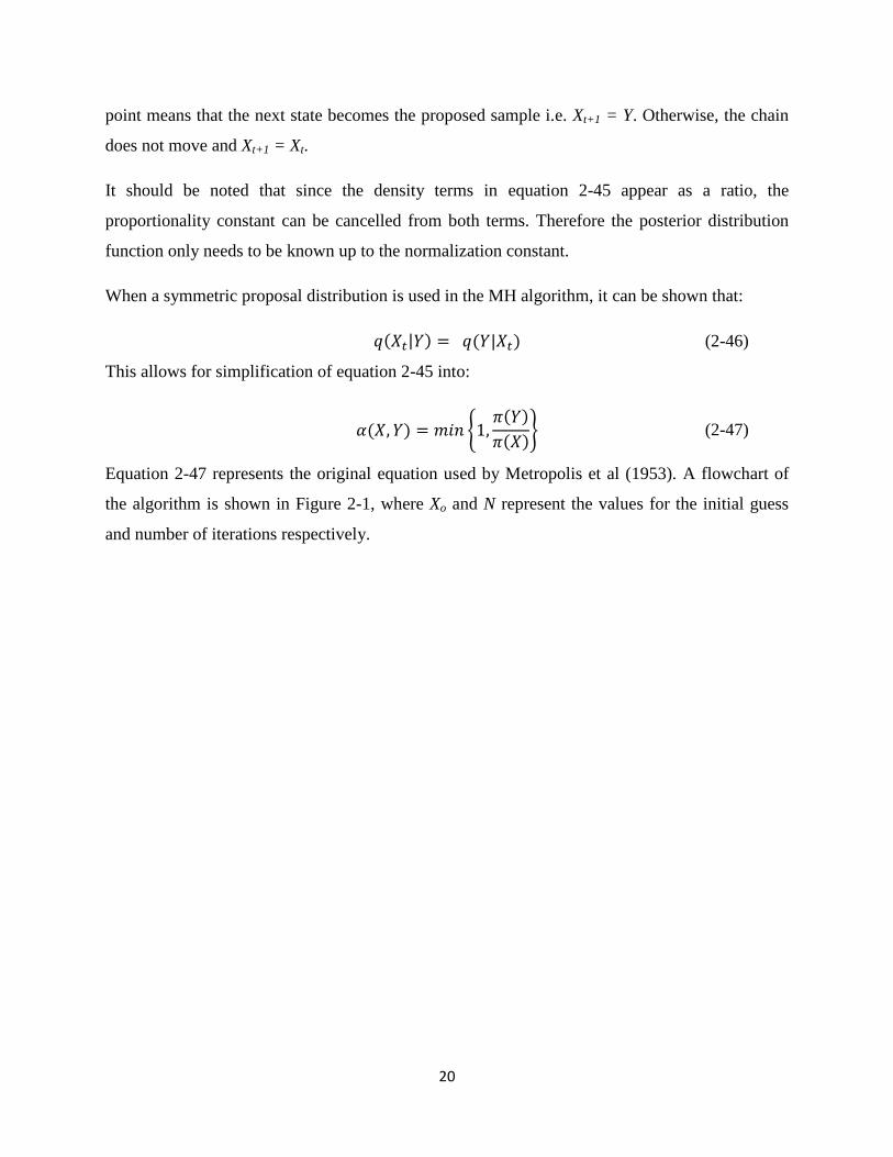
20
point means that the next state becomes the proposed sample i.e. Xt+1 = Y. Otherwise, the chain
does not move and Xt+1 = Xt.
It should be noted that since the density terms in equation 2-45 appear as a ratio, the
proportionality constant can be cancelled from both terms. Therefore the posterior distribution
function only needs to be known up to the normalization constant.
When a symmetric proposal distribution is used in the MH algorithm, it can be shown that:
(2-46)
This allows for simplification of equation 2-45 into:
(2-47)
Equation 2-47 represents the original equation used by Metropolis et al (1953). A flowchart of
the algorithm is shown in Figure 2-1, where Xo and N represent the values for the initial guess
and number of iterations respectively.

21
Figure 2-1: A flowchart describing the Metropolis-Hastings algorithm.

22
Finally, it can be shown that the Metropolis-Hastings algorithm follows the detailed balance
equation. The algorithm can either accept the candidate sample or reject it. Let us consider these
two cases.
Case 1: Xt+1 = Y (The candidate sample was accepted)
The probability of accepting the candidate sample (Y) is:
(2-48)
Recall that the detailed balance equation is given by:
(2-49)
Let us consider the left side of equation 2-49. To prove that the Markov chain obtained from the
MH algorithm satisfies the detailed balance, we can substitute the value for into
equation 2-49. The following expression is then obtained.
(2-50)
(2-51)
The same steps can be now applied to the right side of equation 2-49, and the following equation
can be determined.
(2-52)
Since the proposal distribution is symmetric, equations 2-51 and 2-52 are equal and therefore we
can conclude that the Markov chain for case 1 follows the detailed balance.
Case 2: Xt+1 = Xt (The candidate sample was rejected)
In this case, the chain has not moved and therefore, the next state remains the same as the current
state. It is easy to see that since both states are the same, equation 2-49 will always be satisfied.
Therefore, since the reversibility condition is met in both cases, we can conclude that the MH
algorithm satisfies the detailed balance.

23
Recall from section 2.2.4 that if the Markov chain is found to be reversible, then it has a
stationary distribution. This means that the stationary distribution of the Markov chain obtained
from the MH algorithm is our target distribution.
2.5.2 Single-component Metropolis-Hastings
The original Metropolis-Hastings algorithm updates the entire vector of random variables using
one acceptance/rejection criterion. Sampling all the random variables at once can be problematic
when a larger number of parameters are present. In these situations, it is more convenient to
update each element individually. This is referred to as single-component Metropolis-Hastings.
Suppose we have a vector of random variables that can be divided into r elements.
(2-53)
Now suppose that we want to sample element i at iteration t+1. We can define a vector that
contains all the elements but i.
(2-54)
A candidate value can be generated using the following proposal distribution:
(2-55)
This candidate can be either accepted or rejected based on the Metropolis-Hastings criterion as
shown in equation 2-56.
(2-56)
Although in certain situations, single component sampling can speed up the convergence of the
Markov chain, it should be noted that this method is more demanding computational. The density
values for each component must be calculated; therefore computational time becomes an issue
when the calculations require solving a system of differential equations.
The other issue that needs to be addressed is how to decide on which components to sample
individually and which ones to sample as a block. Gilks et al. (1996) noted that blocking highly
correlated samples together could lead to fast convergence. However, tuning of the proposal
distribution is more effective when the parameters are sampled individually. This idea of

24
blocking will be explored in greater detail through the different chemical engineering case
studies presented in this research.
2.5.3 Random-Walk Metropolis-Hastings
The random-walk Metropolis-Hastings (RWMH) algorithm is a special case of the original MH.
The difference between these two algorithms lies in how the candidate sample is proposed.
Implementation of the RWMH involves proposing a new value, Y, based on the following
equation:
(2-57)
The z term in equation 2-57 represents a random perturbation that can be generated using a
normal distribution. The terms in the above equation become vectors when parameters are
estimated as a block. Other distributions such as the uniform distribution, t-distribution or
triangular distribution can be applied if a normal distribution is deemed insufficient. Based on
equation 2-57, the proposal distribution for the RWMH is of the form:
(2-58)
The idea behind the algorithm is to explore the posterior distribution function in a step-like
manner. Therefore, the size of the perturbation, z, is an important factor that affects the rate of
convergence of the Markov chain. Taking steps that are too small will lead to the chain getting
stuck at certain regions. On the other hand, steps that are too large will result in the chain moving
far out into the tails of the distribution. Tuning of the proposal distribution is explained in greater
detail on section 2.6.1.
2.5.4 Independence Sampler
The candidate sample in the Metropolis-Hastings algorithm can be drawn from a probability
distribution that does not depend on the current state of the Markov chain. In other words,
(2-59)
This type of proposal distribution was first suggested by Tierney (1994) and the algorithm is
referred to as the independence sampler. For this particular proposal, the acceptance criterion
becomes:

25
(2-60)
Since the proposal distribution does not take into account the current state of the Markov chain,
the proposal should closely resemble the target distribution, Therefore, implementation of
this algorithm is only recommended if a good understanding of the posterior distribution is
available. It has also been suggested by Gilks et al. (1996) and later verified by Jarner and
Roberts (2007), that proposal distributions with a heavier tail are better suited when the
independence sampler is applied.
2.5.5 Adaptive MCMC
The MCMC techniques described in the above sections all require some form of tuning. This can
become problematic if the MCMC simulation is computationally intensive. Therefore it would
be ideal if the algorithm can tune itself without any input from the user. This can be
accomplished using an adaptive proposal, where the proposal distribution is changed based on
the previous history of the Markov chain.
Haario et al. (1999), proposed an algorithm that uses an adaptive proposal distribution. The
variance-covariance matrix of the proposal distribution will change throughout the MCMC
routine based on a fixed number of previous states. This adaptive proposal distribution is shown
below:
(2-61)
Where d represents the number of dimension or parameter, cd, represents the scaling factor, and
Rt is the variance-covariance matrix based on a set number of previous trials. The scaling factor,
cd, is often set to be based on the work by Gelman et al. (1996).
The number of states considered when constructing the variance-covariance matrix, Rt, is
controlled by the user. The covariance matrix can be computed using equations 2-62 and 2-63.
(2-62)
where, (2-63)
If we assume that we are using H number of previous states, then K is an H by d matrix, where
each row corresponds to one sample point.

26
It must be emphasized that although the adaptive proposal can achieve convergence, it is not
fully egordic (Haario et al., 1999). Therefore the adaptive proposal is often used to reduce the
size of the burn-in period. The original Metropolis-Hastings or random walk Metropolis-
Hastings algorithm can be implemented once the burn-in period ends.
If application of the adaptive proposal is found to be unsatisfactory, adaptive Metropolis-
Hastings (Haario et al., 2001), can be utilized. This algorithm uses a Gaussian distribution whose
mean is the current state and, whose covariance matrix is updated using all the previous states.
Although the generated Markov chain is non-Markovian due to the adaptive nature of the
algorithm, it was shown to be ergodic under certain conditions (Roberts and Rosenthal, 2007).
2.5.6 The Gibbs Sampler
The Gibbs sampler is a special case of the Metropolis-Hastings algorithm, where all the
candidate samples are accepted. The main advantage of using the Gibbs sampler is that little or
no tuning is required for the Markov chain to converge. However, the algorithm requires fully
conditional probability distributions to be specified for all the parameters. This can be
problematic when the conditional distributions are non-standard and cannot be easily sampled
from. One method of overcoming this complication is to use a conjugate prior (Lee, 2004). When
a conjugate prior is combined with the likelihood, it will produce a standard posterior
distribution that is easy to generate samples from. In situations where the application of
conjugate priors is believed to be unsatisfactory, rejection and resampling methods can be
utilized. These methods are discussed further by Smith (1991) and Smith and Roberts (1993).
The Gibbs sampler was named by Geman and Geman in 1984, who applied the algorithm to an
image restoration problem. Since its proposal, it has been applied in a wide variety of disciplines.
For example, it is frequently used in genetic research for finding specific repeating sequences in
DNA and amino acids (Thijs et al., 2002 and Lawrence et al., 1993). Application of the sampler
in medical research is also prevalent as shown by Gilks et al. (1993) and Scurrah et al. (2003). It
has even been used for modeling hydrological data as shown by Kottegoda et al. (2007). Finally,
Jitjareonchai et al. (2006) applied the Gibbs sampler to chemical engineering problems.
To illustrate the sampling method, first suppose that the vector of random variables , can be
partitioned into r elements as shown below:

27
(2-64)
At time t, the current state of can be expressed as:
(2-65)
and by extension, the next state will be:
(2-66)
Given the joint posterior density function, π( ), the Gibbs algorithm works by updating the
elements of one at a time. The value of the first element Xt+1
1 will be obtained by sampling
from the following fully conditional distribution:
(2-67)
The fully conditional distribution of a parameter can be found by inputting the current values of
all other parameters into the joint probability distribution function. In a similar fashion, the value
of Xt+1
2 is obtained by drawing samples from:
(2-68)
This approach can be continued until all the parameters have been sampled. This algorithm has
been summarized in the flowchart below (Figure 2-2), where Xo and N represent the values for
the initial guess and number of iterations respectively. For more details on the Gibbs sampler, a
comprehensive review has been conducted by Roberts and Smith (1994).

28
Figure 2-2: A flowchart describing the Gibbs Sampler.

29
2.6 Implementation of MCMC
2.6.1 Tuning of Proposal Distribution
The selection of the correct proposal distribution q(.|.), is an essential factor in the convergence
of the Markov chain (Gelman et al. 1996, Roberts et al. 1997 and Gilks et al. 1996). The closer
the proposal is to the target distribution, the faster the Markov chain will enter its stationary
distribution. However, since the shape and size of our target distribution is often unknown, the
chosen proposal distribution must be tuned in order to better resemble our distribution of interest.
Although the Metropolis-Hastings algorithm will converge for a variety of different proposal
distributions, the most commonly used distribution is the normal. In situation where parameters
are sampled as a block, a multivariate normal distribution is utilized. The distribution is usually
centered at the current state of the Markov chain and has a fixed variance-covariance matrix .
Similarly, when the parameters are update individually, a univariate normal with a fixed standard
deviation can be applied.
The efficiency of mixing in a Markov chain is related to the acceptance rate as explained by
Roberts and Rosenthal (2001). Therefore tuning of the proposal distribution is often based on the
acceptance rate of the Markov Chain Monte Carlo algorithm. The term “acceptance rate” refers
to the percent of accepted samples in the MCMC algorithm. Roberts et al. (1997) showed that in
the random walk Metropolis- Hastings algorithm, the optimal acceptance rate is 23.4%. This rate
can be obtained by tuning the elements of the variance-covariance matrix (also known as the
scaling factors) of the proposal distribution.
In general, a high acceptance rate indicates that points at the tails of the distribution are not being
sampled. Therefore increasing the scaling factors will lower the acceptance rate. In a similar
fashion, if a low acceptance rate is detected, the variance of the proposal must be decreased. This
tuning routine can be conducted iteratively in order to achieve good mixing within the chain.
2.6.2 Starting Value
All MCMC algorithms require an initial guess to start the Markov chain. Once the chain enters
its stationary distribution, the MCMC sampling will be independent of the starting value.
However, the speed at which the chain is able to achieve equilibrium depends on how close the
30
initial guess is to the true value of the parameter. Using an initial guess that is well below or
above the true value will require a long Markov chain, and this will result in a high
computational cost.
Determining suitable start points for the Markov chain is an important part in the implementation
of MCMC techniques. If available, prior knowledge about the parameters can be used to provide
a reliable guess. In the absence of prior information, a maximum likelihood estimate can be used
as an initial guess. Another method, proposed by Gelman and Rubin (1992), involves using a
number of different starting values and running several chains in parallel. These “well dispersed”
starting values were obtained by using a mode-finding algorithm that located regions of high
density. The starting values were then generated by sampling from these regions. Brooks (1998),
also recommended applying a simulated annealing technique proposed by Brooks and Morgan
(1994), to generate different starting points for the MCMC algorithm.
2.6.3 Burn-In Period
The period before the Markov chain enters its stationary distribution is referred to as the burn-in
period. The samples in the burn-in period do not belong to the actual posterior distribution;
therefore they must be removed before any statistical inferences can be made. If we assume that
the Markov chain enters the stationary distribution at the mth
iteration, then equation 2-69 can be
used in calculating the expected value.
(2-69)
Determining the length of the burn-in period is often subjective since it is difficult to determine
exactly when the Markov chain has entered its stationary distribution. It has been suggested by
Geyer in 1992 that the burn-in period should be between 1% and 2% of the total chain, given that
the chain is sufficiently long. However, since the burn-in period is depended on the initial guess,
a poor guess can result in a burn-in that is greater than 2% of the chain. A more effective method
is to simply plot the Markov chain time series and visually determine when the chain has reached
equilibrium. This can be difficult for users with little to no experience using MCMC methods.
Therefore, this work will provide examples from different case studies to show how the burn-in
periods can be estimated.

31
2.6.4 Convergence Diagnostics
In implementing Markov Chain Monte Carlo techniques, one question that often arises is when
to stop the Markov chain. Ideally, a Markov chain is said to be converged if the samples have
been drawn from the entire space of the posterior distribution. The difficulty in detecting
convergence lies in the fact that since we do not know the exact shape of our target distribution,
it is difficult to determine whether or not more samples are required. The rest of this section will
provide a brief literature review on different methods used in convergence diagnostics.
One of the problems of using one long chain is that the sampling algorithm might not explore the
entire surface of the posterior distribution (Brooks, 1998). Therefore although the Markov chain
appears to have converged, it might have missed certain regions in the posterior distribution.
This can be overcome by running multiple chains in parallel each with a different starting value.
Comparison of the different Markov chains can then provide a better understanding of
convergence.
Although quantitatively determining whether or not the chain has converged is challenging,
numerous diagnostic techniques have proposed in literature. Raftery and Lewis (1992) used 2-
state Markov chain theory to determine the convergence of one long Markov chain. Gelamn and
Rubin (1992) proposed a convergence diagnostic tool based on the analysis of variance in several
Markov chains. Finally, cumulative sum path plots have been used as a convergence diagnostic
tool by Yu and Mykland (1997). For a more detailed review of the different convergence
diagnostic techniques, please refer to Cowles and Carlin (1996).

32
Chapter 3: Biological Oxygen Demand
3.1 Introduction
The first case study examined in this work is the biological oxygen demand (BOD) problem
reported by Bates and Watts (1988). BOD is a measure of the amount of dissolved oxygen
required by aerobic biological organisms to break down organic materials in water. The
experimental data consists of BOD measurements at seven different times. The oxygen demand
can be modeled as a function of time, and it is often expressed as an exponential decay.
(3-1)
where and are the parameters, x represents the time in days, and is the BOD,
measured in mg/L. The BOD model can also be written in the form of a differential equation.
(3-2)
The purpose of studying the BOD problem is three fold.
1. This chapter will first explore the different steps used in implementing MCMC
techniques in nonlinear models (Figure 3-1). The various implementation factors will be
discussed using specific examples from the BOD case study. The steps presented in this
chapter will provide a general framework for implementing MCMC methods in more
complex models discussed in the subsequent chapters.
2. Another reason for considering the BOD problem is that it has already been studied by
Bates and Watts (1988), where classical regression approaches were applied for
determining parameter point estimates and joint confidence regions. By applying Markov
Chain Monte Carlo techniques, this chapter will provide a comparison between the two
approaches
3. Finally, the BOD problem can be expressed as both an algebraic equation (3-1) and a
differential equation (3-2). Therefore the implementation steps as well as the regression
results from both models can be compared.
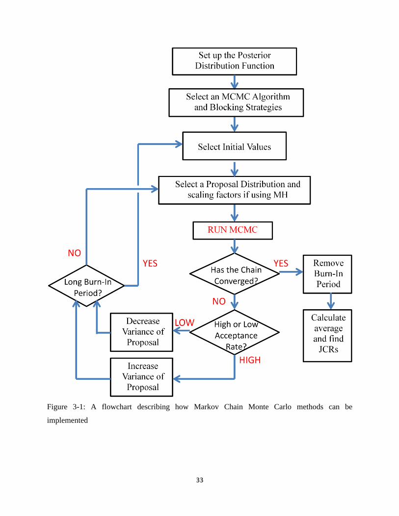
33
Figure 3-1: A flowchart describing how Markov Chain Monte Carlo methods can be
implemented

34
3.2 Implementation of MCMC techniques for the BOD problem
This section will discuss how each of the steps presented in Figure 3-1 can be implemented using
examples from the BOD problem. It should be noted that only the analytical form of the BOD
problem will be considered here.
3.2.1 Development of the Posterior Distribution Function
The first step in using MCMC methods is to set-up the posterior distribution function for the
parameters. Assuming that the measurement error follows a normal distribution, the likelihood
function can be developed as described in section 2.1.2.
(3-3)
Since no prior parameter knowledge was available, a uniform prior distribution was used. The
posterior distribution can then be expressed as:
(3-4)
The posterior distribution contains two model parameters and a pure error variance that needs to
be estimated. Ideally, replicate runs should be used in obtaining an estimate for the pure error
variance. However, in the absence of replicate runs, a value for the variance can be obtained by
treating it as a parameter. The issue of how to correctly estimate the variance will be discussed
further in section 3.3.1.
3.2.2 Selection of MCMC Algorithm and Block Strategies
A variety of different MCMC algorithm are available as described in section 2.5 and deciding on
which algorithm to use can be daunting for users with little MCMC experience. Therefore this
section will explain how to choose the best MCMC technique and illustrate the selection
procedure using the BOD example.
The first step in the selection process is to determine whether or not the conditional probability
density function of the parameters can be expressed as a well-known standard distribution. If this
is possible, the Gibbs sampler technique should be implemented. The advantage of using the

35
Gibbs sampler is that it requires no tuning on the part of the user. In the BOD example, the
conditional probability distribution for the variance parameter can be expressed as the following
Chi-Square distribution:
(3-5)
(3-6)
The conditional distribution for the other two model parameters could not be expressed as a
standard distribution and therefore other MCMC techniques were considered.
The next most efficient MCMC algorithm, after the Gibbs sampler, is the random walk
Metropolis-Hastings or the original Metropolis-Hastings. Both algorithms have the same
implementation difficulty and efficiency as shown by Jitjareonchai (2006). The Metropolis-
Hastings algorithm was chosen for the BOD example, although applying the RWMH would have
produced similar results since the two algorithms differ only in their proposal distributions.
The next step is to decide whether to sample the parameters individually or as a block. It is
recommended that initially, the parameters be estimated individually. The reason for this is that
tuning of the MCMC algorithm becomes difficult if the parameters are sampled together since
only one acceptance rate is observed for all the parameters. By considering the parameters
individually, an acceptance rate for each parameter can be obtained, and the scaling factors can
be tuned accordingly. For this reason, the two parameters in the BOD problem were sampled
separately.
In non-linear models where the tuning of the MH algorithm becomes difficult, an adaptive
MCMC technique can be applied. The algorithm will “adapt” based on the previous values of the
Markov chain. The adaptive MCMC method was not considered for the BOD problem since the
MH algorithm provided adequate results.
To summarize the results so far, the variance can be sampled using the Gibbs sampler, while the
other two parameters in the model can be obtained using the single component MH algorithm.
Once the appropriate MCMC techniques have been selected, the next step is to choose an initial
guess.

36
3.2.3 Selection of Proposal Distribution
The next step in the implementation procedure, as shown in Figure 3-1, is to select the correct
proposal distribution and the corresponding scaling factors. As explained in the previous chapter,
using a proposal distribution that is similar in shape and size to the target distribution is essential
in obtaining good convergence. When little knowledge of the target distribution is known, it is
recommended that a multivariate or univariate normal distribution be selected as the proposal
distribution. Since single component MH was chosen in section 3.2.2, a univariate normal
distribution was utilized.
(3-7)
(3-8)
The normal distribution is centered at the current value of the parameter and has a tunable
variance. The steps involved in tuning will be discussed further in section 3.2.6. The next section
will examine in detail the specific steps in the proposed MCMC algorithm.
3.2.4 Selection of Initial Values and Burn-in Period
The length of the burn-in period is determined by how close the initial guess is to the actual
parameter value. As discussed in section 2.6.2, the initial guess can either be estimated from
previous knowledge or determined using the techniques reviewed by Brooks (1998). In many
estimation problems, even a poor initial guess can lead to a quick convergence of the Markov
chain to its stationary distribution. Consider the figure below, where an initial guesses of 35 and
3 were used for parameter 1 and 2, respectively. The plot represents a discrete time series, where
the values of parameters 1 and 2 at each cycle are shown. This visual representation of the
Markov chain is often helpful in determining when the chain enters its stationary phase.

37
Figure 3-2: The Markov chain for the first 1000 cycles when an initial guess of 35 and 3 were
used for parameters 1 and 2 respectively in the BOD model. The line represents the time when
the burn-in period ends and the stationary distribution begins.
A time series is stationary if its mean value does not change over time. Therefore by visual
inspection, it appears that the Markov chain has entered its stationary distribution after the first
100-200 cycles. That is, the mean of the time series after this period does not appear to change
with time. Therefore the burn-in period in this problem is only the first 100-200 cycles. After this
period, the Markov chain does not depend on the initial value. The samples from the burn-in
period can be removed and the remaining samples can be used to calculate the mean and joint
confidence regions.
Although the Markov chain reached equilibrium quickly for the BOD problem, the mixing of the
chain might be more challenging in other non-linear problems. If a large burn-in period is
observed, changing the initial guess can often improve the convergence. One strategy is to
simply start the Markov chain where the previous one ended. Although poor initial guesses can
sometimes lead to a Markov chain that is non-stationary, it should be noted that optimization
algorithms also require a suitable initial guess. Therefore, the problem of obtaining a good initial
guess is present regardless of what regression methodology is being applied.
0 100 200 300 400 500 600 700 800 900 100010
15
20
25
30
35
40
MCMC Cycle
Par
amet
er 1
0 100 200 300 400 500 600 700 800 900 10000
1
2
3
4
MCMC Cycle
Par
amet
er 2

38
3.2.5 MCMC Algorithm Steps
In the algorithm selection process, the Gibbs sampler and Metropolis-Hastings algorithm were
proposed in estimating the variance and the model parameters, respectively. The main steps in
the sampling procedure are described below:
1. Calculate the sum of squared error using equation 3-6 and the initial values of the other
two parameters and .
2. Draw a sample from the Chi-Square distribution with n degrees of freedom. In this
particular example, n = 6 since six experimental runs were carried out.
3. Determine the value for by rearranging equation 3-5.
(3-9)
4. Generate a candidate value for parameter 1, , in the BOD model using the proposal
distribution described in section 3.2.4. The candidate is accepted or rejected based on the
following criterion.
(3-10)
5. Generate another candidate value for parameter 2, , in a similar fashion as the previous
step. Again the candidate is either accepted or rejected based on the following criterion.
(3-11)
6. Return to step 1 and continue iteration until the Markov chain converges to its stationary
distribution.
3.2.6 Tuning
The tuning of the proposal distribution is an important step in obtaining reliable parameter
estimates and joint confidence regions. The standard deviation of the proposal needs to be
adjusted until a good acceptance rate is obtained. Roberts (1997) showed that an acceptance rate
around 23% produces the most efficient Markov chain. In practice however, it is very difficult to
obtain exactly 23%, especially when the algorithm is computationally intensive. Jitjareonchai
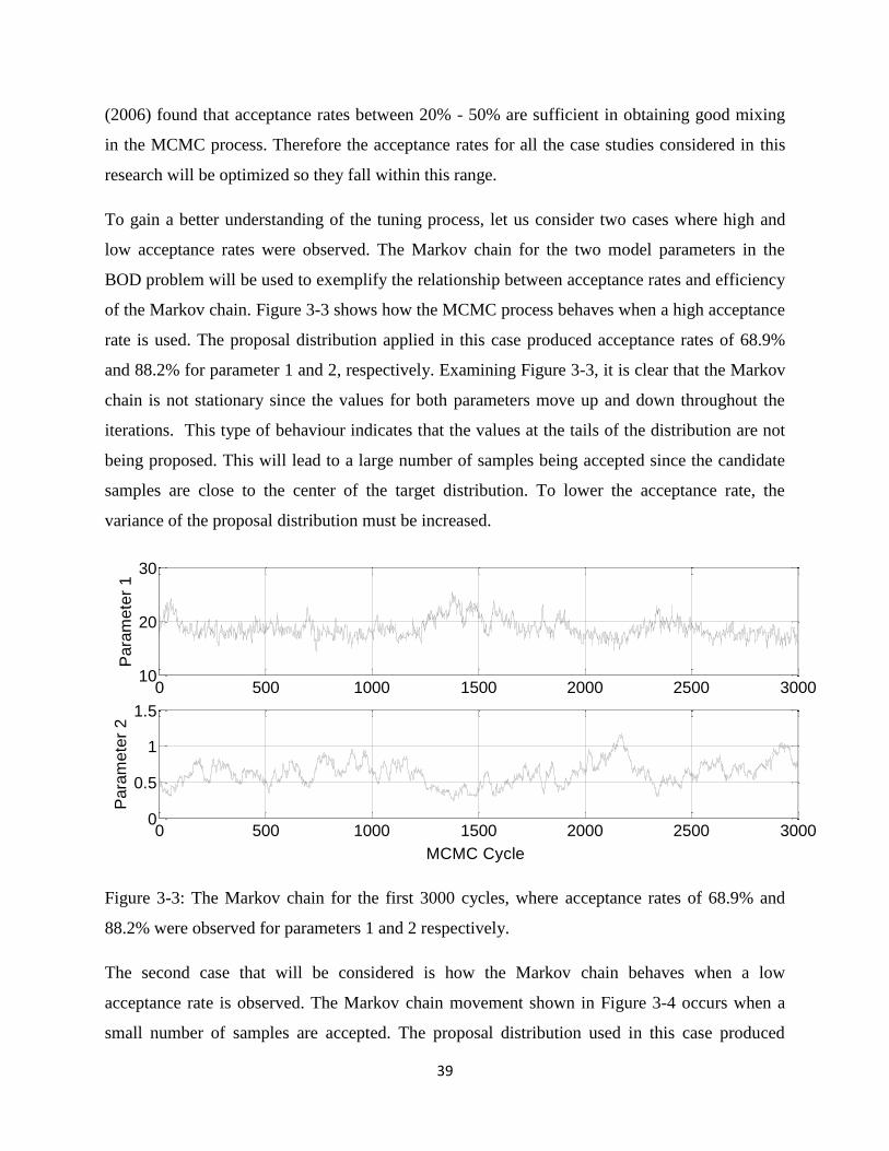
39
(2006) found that acceptance rates between 20% - 50% are sufficient in obtaining good mixing
in the MCMC process. Therefore the acceptance rates for all the case studies considered in this
research will be optimized so they fall within this range.
To gain a better understanding of the tuning process, let us consider two cases where high and
low acceptance rates were observed. The Markov chain for the two model parameters in the
BOD problem will be used to exemplify the relationship between acceptance rates and efficiency
of the Markov chain. Figure 3-3 shows how the MCMC process behaves when a high acceptance
rate is used. The proposal distribution applied in this case produced acceptance rates of 68.9%
and 88.2% for parameter 1 and 2, respectively. Examining Figure 3-3, it is clear that the Markov
chain is not stationary since the values for both parameters move up and down throughout the
iterations. This type of behaviour indicates that the values at the tails of the distribution are not
being proposed. This will lead to a large number of samples being accepted since the candidate
samples are close to the center of the target distribution. To lower the acceptance rate, the
variance of the proposal distribution must be increased.
Figure 3-3: The Markov chain for the first 3000 cycles, where acceptance rates of 68.9% and
88.2% were observed for parameters 1 and 2 respectively.
The second case that will be considered is how the Markov chain behaves when a low
acceptance rate is observed. The Markov chain movement shown in Figure 3-4 occurs when a
small number of samples are accepted. The proposal distribution used in this case produced
0 500 1000 1500 2000 2500 300010
20
30
Para
mete
r 1
0 500 1000 1500 2000 2500 30000
0.5
1
1.5
MCMC Cycle
Para
mete
r 2
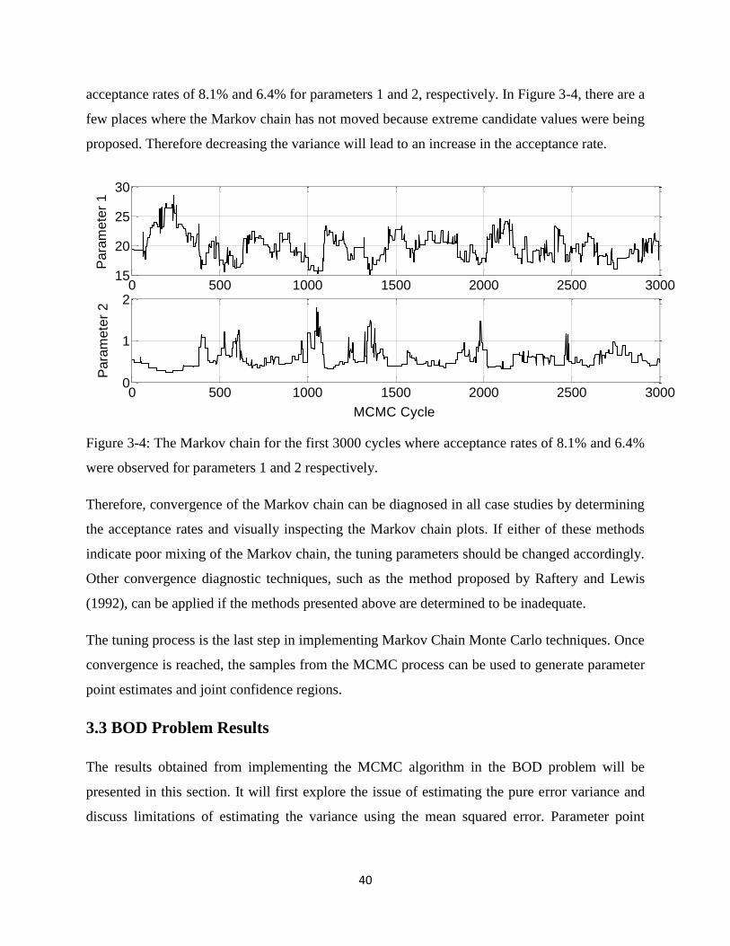
40
acceptance rates of 8.1% and 6.4% for parameters 1 and 2, respectively. In Figure 3-4, there are a
few places where the Markov chain has not moved because extreme candidate values were being
proposed. Therefore decreasing the variance will lead to an increase in the acceptance rate.
Figure 3-4: The Markov chain for the first 3000 cycles where acceptance rates of 8.1% and 6.4%
were observed for parameters 1 and 2 respectively.
Therefore, convergence of the Markov chain can be diagnosed in all case studies by determining
the acceptance rates and visually inspecting the Markov chain plots. If either of these methods
indicate poor mixing of the Markov chain, the tuning parameters should be changed accordingly.
Other convergence diagnostic techniques, such as the method proposed by Raftery and Lewis
(1992), can be applied if the methods presented above are determined to be inadequate.
The tuning process is the last step in implementing Markov Chain Monte Carlo techniques. Once
convergence is reached, the samples from the MCMC process can be used to generate parameter
point estimates and joint confidence regions.
3.3 BOD Problem Results
The results obtained from implementing the MCMC algorithm in the BOD problem will be
presented in this section. It will first explore the issue of estimating the pure error variance and
discuss limitations of estimating the variance using the mean squared error. Parameter point
0 500 1000 1500 2000 2500 300015
20
25
30
Para
mete
r 1
0 500 1000 1500 2000 2500 30000
1
2
MCMC Cycle
Para
mete
r 2

41
estimates and JCRs will then be generated from the MCMC samples and a comparison of the
MCMC results with the classical regression approaches will be presented.
3.3.1 Issue with the Error Variance
The results from the BOD problem illustrate the importance of correctly estimating the error
variance when using an MCMC approach. In the absence of replicate runs, the error variance can
be determined from the mean squared error (MSE) or it can be estimated as a parameter in the
regression problem. The problem in using the former approach to estimate the error is that in a
non-linear model, the mean squared error is not an unbiased estimator of the pure error variance.
Therefore, a more precise estimate of the pure error can be attained by treating the variance as a
parameter. The limitations of using the MSE will be exemplified using the BOD case study.
Using the parameter estimates from Bates and Watts (1988), the mean squared error was found
to be 6.484 with 4 degrees of freedom. The MCMC protocol shown in Figure 3-1 was then
implemented using the MSE as an estimate for . However, upon using this fixed value for the
measurement error, convergence of the Markov chain could not be achieved.
Recall from section 3.2.6 that convergence can be diagnosed using both the acceptance rates and
the Markov chain time series plots. For this particular problem, acceptance rates of 66% and
95% were observed for parameters 1 and 2 respectively. The acceptance rates in these results are
much higher than the acceptable range of 20-50%. Normally, if a high acceptance rate is
observed, the variance of the proposal can be increased to lower the rate. However, in this
particular problem, changing the scaling factors was found to have minimal effect on the
acceptance rate.
The Markov chain time series was also generated for the purposes of convergence diagnostics
(Figure 3-5). It can be seen from the graph that parameter 1 values are gradually increasing after
the first 1,000,000 runs, while unrealistic values of parameter 2 are being sampled in the initial
stages of the Markov chain. This erratic movement indicates that the chain has not converged to
its stationary distribution. Although several different proposal distributions and scaling factors
were applied, the mixing of the Markov chain did not improve.

42
Figure 3-5: The MCMC output for the two parameters in the BOD problem. The parameter
values sampled at each iteration is shown above for the first 2,000,000 cycles.
To understand why the Markov chain did not converge to its stationary distribution when using
the mean squared error, consider Figure 3-6 shown below. The value for parameter 2 was held
constant at 19.16, while parameter 1 was varied from 0.15 to 6. Using this range and a variance
of 6.484, the value proportional to the density of the posterior distribution was determined and
plotted as a function of parameter 1. It can be seen from Figure 3-6, that the distribution of
parameter 1 at a parameter 2 value of 19.16 has a very long tail. Therefore one possible
explanation for the lack of convergence in the MCMC algorithm is that the Markov chain is
becoming stuck in the tail of the distribution.
Figure 3-6: Values proportional to the density of the posterior obtained using parameter 1 values
from 0.15 to 6 and a fixed parameter 2 value of 19.16. The pure error variance was estimated
using the MSE.
0 0.2 0.4 0.6 0.8 1 1.2 1.4 1.6 1.8 2
x 106
0
200
400P
ara
me
ter
2
0 0.2 0.4 0.6 0.8 1 1.2 1.4 1.6 1.8 2
x 106
0
5
10
MCMC Cycle
Pa
ram
ete
r 1
0 1 2 3 4 5 60
0.2
0.4
0.6
0.8
Parameter 1
Pro
po
rtio
na
l to
De
nis
ty

43
In order to explain why the Markov chain is becoming stuck in the tail of the posterior
distribution, consider Table 3-1. The table shows six sample MCMC iterations starting from a
parameter 1 value of 3. Candidate samples are then proposed and the transition probabilities α, is
calculated by dividing the density at the proposed sample by the density at the current sample.
Notice that the transition probabilities for every iteration is higher than 0.9. This is because the
density at the current value is close to the density at the proposed value. A high transitional
probability means that a large number of candidate samples will be accepted, and this can cause
the Markov chain to move further and further into the tail of the distribution. This is one possible
reason for the gradual increase in parameter 1 observed in Figure 3-5.
Table 3-1: Possible values for the current and candidate samples
Iteration
Current Value
of the Markov
chain
Proposed
Value
Density of
Posterior at
Current
Value
Density of
Posterior at
Proposed
Value
Transitional
Probability
α
1 3.00 3.12 0.0941 0.0915 0.973
2 3.12 3.20 0.0915 0.0900 0.983
3 3.20 3.32 0.0900 0.0880 0.978
4 3.32 3.50 0.0880 0.0854 0.971
5 3.50 4.50 0.0854 0.0778 0.910
6 4.50 6.00 0.0778 0.0778 0.958
Now consider the second approach for estimating the pure error, where the error variance is
treated as a parameter. The MCMC algorithm was be implemented as described in section 3.2
and the Markov chain for parameter 1, parameter 2 and the error variance is shown in Figure 3-7.
Examination of the time series reveals that the mean value for all three parameters remains
constant throughout. Therefore it appears that the Markov chain has converged to its stationary
distribution. Acceptance rates of 30% and 35% were obtained for parameter 1 and 2,
respectively, again indicating good mixing of the Markov chain.

44
Figure 3-7: The MCMC output for the two model parameters in the BOD problem and the error
variance.
The samples for the variance were generated using the Gibbs sampler and after taking the
average of these MCMC samples, a variance estimate of 2.34 was obtained. Comparison to the
MSE approach reveals a much smaller variance. The difference in variance has a large impact of
the broadness of the posterior distribution as illustrated in Figure 3-8.
0 1 2 3 4 5 6 7 8 9 10
x 104
0
10
20
Va
rain
ce
0 1 2 3 4 5 6 7 8 9 10
x 104
0
20
40
Pa
ram
ete
r 1
0 1 2 3 4 5 6 7 8 9 10
x 104
0
5
Pa
ram
ete
r 2

45
Figure 3-8: Values proportional to the density of the posterior obtained using parameter 1 values
from 0.15 to 1.2 and a fixed parameter 2 value of 19.16. The pure error variance was estimated
by treating the variance as a parameter.
The above figure was constructed using the same methodology as Figure 3-5, only the new
variance value of 2.34 was used. It can be seen that the long broad tail that was present in the
Figure 3-5 is no longer an issue. Therefore by estimating the variance using the MCMC protocol,
more reliable results were obtained.
There are two key take-away points from these results presented so far in this section. First,
using the MSE to determine the pure error variance was found to give unpredictable results.
Estimating the variance along with the other two parameters is a better approach since
uncertainty in the model parameters are taken into consideration in the estimation procedure.
Therefore, the results shown in this work illustrate the importance of treating the variance as a
parameter to be estimated rather than fixing its value based on the mean squared error. Second,
the findings from this work indicate that when the variance is large and the posterior distribution
has a large tail, MCMC algorithms can sometimes have difficulty in achieving convergence. In
these situations, the density values for the current state and the candidate samples will be close to
each other and therefore high acceptance rates are often encountered. To prevent the Markov
0 0.2 0.4 0.6 0.8 1 1.2 1.40
0.01
0.02
0.03
0.04
Parameter 1
Pro
po
rtio
na
l to
De
nsity

46
chain from becoming stuck in the tails of the distribution, a carefully designed adaptive proposal
distribution might have to be implemented.
3.3.2 Parameter Estimates and Joint Confidence Regions
The parameter point estimates can be determined by taking the average of the MCMC samples.
A comparison of these results with the Gauss-Newton optimization used by Bates and Watts is
shown in Table 3-2.
Table 3-2: The point estimates for parameters in the BOD problem using the Gauss-Newton and
MCMC optimization techniques. The variance for the Gauss-Newton optimization is based on
the MSE
Gauss-Newton
Optimization
Estimate
MCMC
Estimate
Parameter 1 19.157 19.17
Parameter 2 0.5511 0.5942
Variance 6.484* 2.34
From Table 3-2, it can be seen that both regression methods produce similar parameter estimates
for parameter 1 and 2. The slight difference in the values could be due to the fact that MCMC
estimates are based on taking the expected value while the Gauss-Newton optimization attempts
to find the mode of the posterior distribution.
In addition to the parameter values, joint confidence regions can also be constructed for
parameters 1 and 2. These regions represent all the possible values for parameter 1 and 2 at a
fixed confidence level. The size of the JCRs represents the precision in the parameter estimates
while rotation away from the y-axis indicates correlation between the parameters.
The first step in generating JCRs is to use the samples obtained from the MCMC algorithm to
create a 3-dimensional histogram. This histogram for a 2 parameter model presents the actual
posterior distribution function of the parameters. Therefore a contouring algorithm can be
applied to the histogram in order to construct the 95% confidence region.

47
One of the objectives of this research is to compare the Markov Chain Monte Carlo JCRs with
the JCRs obtained from the approximation techniques discussed in section 2.3. First let us
consider the confidence region from the elliptical approximation, where linear regression theory
is used. This problem was studied by Bates and Wates (1988) and the elliptical JCR is shown in
Figure 3-9.
Figure 3-9: Parameter estimates and 95% joint confidence regions obtained using an elliptical
approximation and Markov Chain Monte Carlo techniques.
The correct size and shape of the joint confidence region is represented by the MCMC curve in
Figure 3-9. Comparison of the two methods in Figure 3-9 reveals two major limitations of using
the elliptical approximation. First, the approximate JCR in Figure 3-9 has a much larger
confidence region when compared to the MCMC approach. The region also contains unrealistic
parameter 2 values below zero. Therefore the results indicate that applying linear regression
theory to the BOD problem will result in an overestimation of the parameter uncertainty. Second,
since the model is highly non-linear, the elliptical approach is not able to adequately capture the
shape of the JCR. The true shape of the confidence region, as shown by the MCMC plot, cannot
be modeled by using an ellipse. Therefore, an MCMC approach needs to be utilized in the BOD
problem in order to attain correct shape and probability content JCRs.
Parameter 1
Para
mete
r 2
10 15 20 25 30 35-0.5
0
0.5
1
1.5
2Elliptical Approximation JCR
MCMC JCR
Parameter estimate, Gauss Newton
Parameter estimate, MCMC

48
Since Figure 3-9 indicates that the shape of the JCR is non-elliptical, the exact shape method
from section 2.3.2 was applied. When using this method, a root finding algorithm needs to be
used to determine the confidence region. The exact shape JCR plot along with the MCMC JCR is
depicted in Figure 3-10.
Figure 3-10: 95% joint confidence regions obtained using an exact shape approximation and
Markov Chain Monte Carlo techniques.
Using the exact shape method, the correct shape of the JCR is observed in Figure 3-10. However
notice that the confidence region does not close at the top or at the bottom. Complex numbers
were encountered when the root finding algorithm was implemented in these regions. Therefore
comparison of the two plots reveals that the exact shape JCRs do not have the correct probability
content. This example serves to further exemplify the advantage of using MCMC techniques in
non-linear models.
3.4 BOD Problem Using the Differential Form
The BOD problem represents an interesting case, where the model can be expressed in both the
analytical and differential form. The differential equations encountered in subsequent chapters
Parameter 1
Para
mete
r 2
10 15 20 25 30 35-0.5
0
0.5
1
1.5
2Exact Shape Upper Curve
Exact Shape Lower Curve
MCMC JCR

49
will not have a closed form solution. Therefore, the BOD problem represents a unique
opportunity to compare the computational time and implementation steps for both forms of the
model.
3.4.1 Implementation
Implementation of the differential form of the BOD problem can be accomplished using the
same algorithm shown in section 3.2.5. The only difference is that calculating the posterior
density function in equations 3-10 and 3-11 now require solving the differential equation. The
posterior density in the BOD problem can be calculated using the following steps.
1. Determine a time step for solving the differential equation numerically. Although a small
time step will produce a more accurate result, it will also require greater computational
time. Therefore careful selection of the step size is an essential part of the implementation
process.
2. There are a variety of methods available for solving differential equations numerically. In
this research, since all coding was accomplished using Matlab software, the Matlab
built-in function ODE 45 was utilized. The built in function uses a Runge-Kutta
algorithm with a variable time step for efficient computation.
3. Using ODE 45, the predicted BOD value, , can be determined for each
experimental run in the data. The density is then calculated based on the following
equation.
(3-12)
The parameter point estimates and joint confidence regions obtained using both form of the BOD
model are shown in Figure 3-11.

50
Figure 3-11: 95% joint confidence regions obtained using the differential and analytical forms of
the BOD model.
The JCRs and point estimates obtained when using the differential form of the model are almost
the same as the results found from using the analytical equation. Therefore, the proposed
algorithm for solving models with differential equations is valid, and the algorithm will be
applied in the following chapters.
3.5 Summary
A MCMC implementation methodology was present in this chapter using specific examples from
the BOD case study. The chapter focused on choosing the proper MCMC technique, selecting
the approximate starting values, properly detecting convergence of the Markov chain and
correctly tuning the MCMC algorithm. In addition, the results also showed that the pure error
variance needs to be estimated as a parameter in order to obtain correct results. Once the MCMC
algorithm was implemented successfully, the results were then compared with approximation
techniques. It was found that both approximation methods of constructing JCRs yielded incorrect
results. Therefore MCMC methods must be used in these non-linear models. Finally, good
agreement was observed between the analytical and differential forms of BOD model.
Parameter 1
Para
mete
r 2
16 18 20 22 24 26 28
0.2
0.4
0.6
0.8
1
1.2
1.4 Differential form BOD
Analytical form BOD

51
Chapter 4: Reactivity Ratio Estimation
4.1 Introduction
Polymerization processes represent an important approach to the production of a wide variety of
industrially important materials. It is of practical importance to study these systems in order to
produce polymeric materials with the desired properties. Investigation of these systems is also
essential to the control and safe and efficient operation of polymerization reactors. Modeling
these reactions, however, requires knowledge of polymerization parameters such as reactivity
ratios. To define reactivity ratios, first let us consider the reaction below.
(4-1)
where denotes monomer j, represents a propagating copolymer radical with n monomer
units and the last unit containing monomer i. For a copolymer system, i and j can take on values
of 1 and 2. Using the four propagating rate constant, the reactivity ratios can be defined as shown
below.
(4-2)
(4-3)
Although a significant number of studies have been carried out for reactivity ratio estimation in
copolymerization systems, these studies fail to accurately capture the uncertainty in the
parameters. The confidence regions presented in these studies are often approximate in shape and
probability content as seen in Chapter 3. The failure of these methods to accurately capture the
uncertainty depends upon the non-linearity of the model and the design of the data. The joint
confidence regions developed using MCMC methods therefore can improve upon parameter
uncertainty estimates and can provide insights into how accurate the approximation techniques
are.
Reactivity ratios can be determined using either copolymer composition data or triad fraction
data. When copolymer composition data is available at low conversion, the Mayo-Lewis model
is applied. For higher conversion, the Meyer Lowry model and the direct numerical integration

52
scheme are applied. On the other hand, when triad fraction data is available, a multiresponse
estimation scheme must be utilized. In this chapter, reactivity ratios and joint confidence regions
will be estimated in the four options listed above. In doing so, the following two objectives will
be addressed:
1. The MCMC implementation framework provided in chapter 3 will be applied to the four
cases listed above. Regression analysis in these cases involves solving implicit equations,
differential equations and dealing with multiple responses. Therefore this chapter
presents an opportunity to explore in detail, the required MCMC implementation steps
for these different aspects in non-linear models.
2. The parameter estimates and joint confidence regions obtained using the MCMC
methodology will be compared to the approximation methods discussed in section 2.3.
The comparison will provide a better understanding of whether or not the approximate
joint confidence region can adequately capture parameter uncertainty. When these
approximations fail, MCMC methods must be used. Therefore, the case studies will
attempt to illustrate the advantage of using MCMC techniques when analyzing non-linear
models in chemical engineering problems.
4.2 Copolymer Composition Data
The copolymer composition data used in this work was taken from Madruga and Fernandez-
Garcia (1994), who studied the free radical copolymerization of di-n-butyl itaconate (DBI) and
methyl methacrylate (MMA). This system was previously studied by Kazemi et al. (2011) and
comparison of their results with the MCMC results will be provided. The free radical
copolymerization was carried out in benzene at 50ºC and at low conversion levels. Sixteen
experimental trials were conducted at various monomer feed composition f10, and conversion
levels Xw, and the output copolymer composition , was measured.

53
Table 4-1: Experimental data for DBI/MMA copolymerization at low conversion level (Madruga
and Fernandez-Garcia, 1994)
Feed composition
f10
Conversion Xw
(wt%)
Copolymer
composition
0.035 6.46 0.025
0.064 6.04 0.043
0.065 8.05 0.056
0.199 5.34 0.165
0.301 5.09 0.246
0.301 5.97 0.259
0.499 3.61 0.377
0.453 8.77 0.382
0.491 3.86 0.411
0.547 4.18 0.459
0.599 3.17 0.512
0.698 4.47 0.623
0.798 4.64 0.732
0.301 4.82 0.272
0.492 4.05 0.416
0.7 4.75 0.628
Although the initial monomer feed and conversion levels represent the independent variable, the
error associated with them cannot be neglected. Therefore an error in variables (EVM) model
was applied to the Mayo-Lewis model, the Meyer Lowry model and the direct numerical
integration model. The data set shown in Table 4-1 will be used for all three models. The
following sections will discuss the implementation steps and present the MCMC results from
each of the three models.

54
4.2.1 Error Structure
Prior to setting up the EVM model, assumptions regarding the error structure for both the
independent and dependent variables must be established. It is assumed that all measurements
are independent, and that the error for all variables is normally distributed. Determining the
magnitude of the error often necessitate running replicate experiments. When replicates are not
present, literature sources or past experience can provide a guideline for the magnitude of the
errors. For this particular case study, the error will be assumed to be multiplicative at levels of
±1, ±1, and ±5 for variables f10, Xn, and respectively.
(4-1)
(4-2)
(4-3)
The asterisk represents the true values of the variables and is the error term for each variable.
In order to express the above equations in a more convenient form, the natural logarithm can be
taken of both sides. At low error levels, the term ln(1+ can be approximated by and the
above equations can be simplified to:
(4-4)
(4-5)
(4-6)
4.2.2 Mayo-Lewis Model
The Mayo-Lewis model, shown in equation 4-7, provides a relationship between the true values
of the instantaneous copolymer composition, the unreacted monomer composition, and the
reactivity ratios (Mayo and Lewis, 1944). The model assumes that the monomer composition
does not change with conversion. Therefore the model is only valid at low conversion levels
since compositional drift can occur as the polymerization reaction progresses.

55
(4-7)
The implementation protocol described in Chapter 3 can now be applied to the Mayo-Lewis
model. Error in both the unreacted monomer composition f1, and the instantaneous copolymer
composition F1, will be considered. The posterior distribution function can then be developed by
combining the EVM likelihood function shown in Chapter 2, equation 2-24, with a uniform
prior.
(4-8)
where and
represent the true values of the measurements that need to be estimated. Since
the reactivity ratios are of primary interest, equation 4-7 can be substituted for in equation 4-8.
(4-9)
The regression approach involves estimating 16 parameters and two reactivity ratio
parameters. This can be accomplished using the Metropolis-Hastings algorithm. When
considering what blocking scheme to use, recall from Chapter 2 that correlated parameters
should be estimated simultaneously. Therefore, the parameters can be sampled as one block,
and the reactivity ratios can be sampled as another block. The Markov chain can be generated by
following the procedure below.
1. Generate 16 values for using a multivariate normal distribution, where the mean is the
current state of the Markov chain. The elements of the covariance matrix of the proposal
distribution are tuned based on the acceptance rate.
2. Accept or reject all 16 values of based on the following acceptance criterion:
56
(4-10)
Note R in the above equation represents the values of r1 and r2.
3. Generate values for r1 and r2 using a multivariate normal distribution. Again the
distribution should be centered at the current value of the Markov chain.
4. Accept or reject both r1 and r2 values based on the following criterion:
(4-11)
5. Return to step 1 and continue the MCMC cycle until convergence is achieved.
Note that in the subsequent sections when the EVM variable is introduced, steps 1 and 2 are
repeated for this additional variable.
Acceptance rates of 22 % and 33% were observed indicating that the Markov chain appears to
have successfully converged to its stationary distribution. Another method of checking
convergence is to start at extreme initial values and see if the chain settles down. As shown in
Figure 4-1 below, even when an initial guess of 1.5 and 2 was used for the two reactivity ratios,
the Markov chain quickly reached equilibrium.

57
Figure 4-1: The MCMC output for the two reactivity ratios in the Mayo-Lewis equation using an
initial guess of 1.5 and 2 was used for parameters 1 and 2 respectively. The first 500 cycles
represents the burn-in period that occurs due to the initial guess.
After executing the sampling procedure for 1,000,000 cycles, the average of the samples was
taken in order to determine the reactivity ratios. Table 4-2 shows the MCMC results along with
the optimization estimates from Kazemi et al. (2011). There is excellent agreement between the
two methods, indicating reliable parameter estimates can be attained using both methods.
0 500 1000 1500 2000 2500 3000
0.6
0.8
1
1.2
1.4
1.6
MCMC Cycle
r1
0 500 1000 1500 2000 2500 3000
1.4
1.6
1.8
2
MCMC Cycle
r2
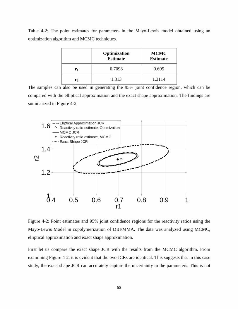
58
Table 4-2: The point estimates for parameters in the Mayo-Lewis model obtained using an
optimization algorithm and MCMC techniques.
Optimization
Estimate
MCMC
Estimate
r1 0.7098 0.695
r2 1.313 1.3114
The samples can also be used in generating the 95% joint confidence region, which can be
compared with the elliptical approximation and the exact shape approximation. The findings are
summarized in Figure 4-2.
Figure 4-2: Point estimates and 95% joint confidence regions for the reactivity ratios using the
Mayo-Lewis Model in copolymerization of DBI/MMA. The data was analyzed using MCMC,
elliptical approximation and exact shape approximation.
First let us compare the exact shape JCR with the results from the MCMC algorithm. From
examining Figure 4-2, it is evident that the two JCRs are identical. This suggests that in this case
study, the exact shape JCR can accurately capture the uncertainty in the parameters. This is not
0.4 0.5 0.6 0.7 0.8 0.9 11
1.2
1.4
1.6
r1
r2
Elliptical Approximation JCR
Reactivity ratio estimate, Optimization
MCMC JCR
Reactivity ratio estimate, MCMC
Exact Shape JCR
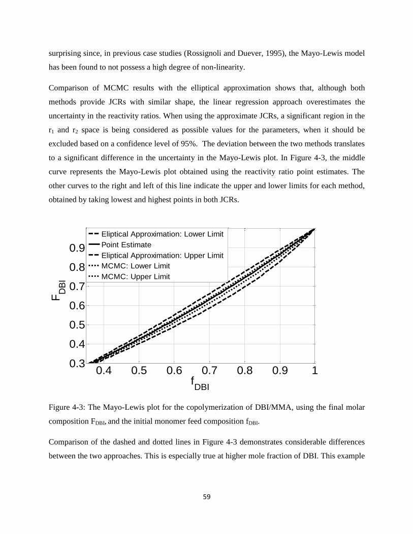
59
surprising since, in previous case studies (Rossignoli and Duever, 1995), the Mayo-Lewis model
has been found to not possess a high degree of non-linearity.
Comparison of MCMC results with the elliptical approximation shows that, although both
methods provide JCRs with similar shape, the linear regression approach overestimates the
uncertainty in the reactivity ratios. When using the approximate JCRs, a significant region in the
r1 and r2 space is being considered as possible values for the parameters, when it should be
excluded based on a confidence level of 95%. The deviation between the two methods translates
to a significant difference in the uncertainty in the Mayo-Lewis plot. In Figure 4-3, the middle
curve represents the Mayo-Lewis plot obtained using the reactivity ratio point estimates. The
other curves to the right and left of this line indicate the upper and lower limits for each method,
obtained by taking lowest and highest points in both JCRs.
Figure 4-3: The Mayo-Lewis plot for the copolymerization of DBI/MMA, using the final molar
composition FDBI, and the initial monomer feed composition fDBI.
Comparison of the dashed and dotted lines in Figure 4-3 demonstrates considerable differences
between the two approaches. This is especially true at higher mole fraction of DBI. This example
0.4 0.5 0.6 0.7 0.8 0.9 10.3
0.4
0.5
0.6
0.7
0.8
0.9
fDBI
FD
BI
Eliptical Approximation: Lower Limit
Point Estimate
Eliptical Approximation: Upper Limit
MCMC: Lower Limit
MCMC: Upper Limit
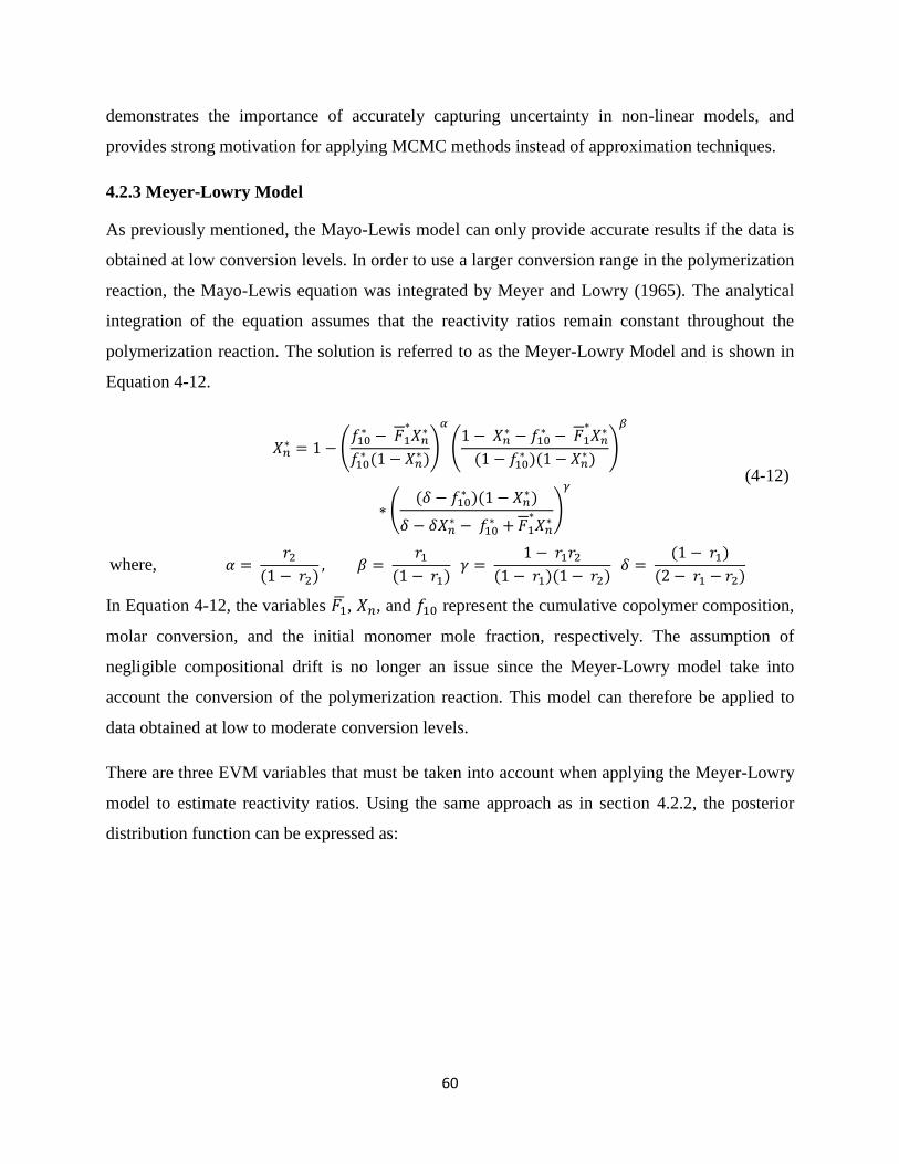
60
demonstrates the importance of accurately capturing uncertainty in non-linear models, and
provides strong motivation for applying MCMC methods instead of approximation techniques.
4.2.3 Meyer-Lowry Model
As previously mentioned, the Mayo-Lewis model can only provide accurate results if the data is
obtained at low conversion levels. In order to use a larger conversion range in the polymerization
reaction, the Mayo-Lewis equation was integrated by Meyer and Lowry (1965). The analytical
integration of the equation assumes that the reactivity ratios remain constant throughout the
polymerization reaction. The solution is referred to as the Meyer-Lowry Model and is shown in
Equation 4-12.
(4-12)
where,
In Equation 4-12, the variables , , and represent the cumulative copolymer composition,
molar conversion, and the initial monomer mole fraction, respectively. The assumption of
negligible compositional drift is no longer an issue since the Meyer-Lowry model take into
account the conversion of the polymerization reaction. This model can therefore be applied to
data obtained at low to moderate conversion levels.
There are three EVM variables that must be taken into account when applying the Meyer-Lowry
model to estimate reactivity ratios. Using the same approach as in section 4.2.2, the posterior
distribution function can be expressed as:

61
(4-13)
Note that the expression
is used since the Meyer-Lowry model is in the form of
an implicit equation; therefore, an analytical expression for cannot be obtained. This requires
the implementation of a root finding algorithm in order to find the value of at the particular
experimental trial.
Finding parameter estimates in the Meyer-Lowry model once again necessitates using the MH
algorithm. The same implementation steps that were carried out in the Mayo-Lewis model can be
applied here, with two key differences. First, there is an additional EVM variable ; therefore
another multivariate normal distribution must be used to generate 16 samples for the conversion.
The acceptance criterion can then be set up using the current values of the other parameters.
Second, there is a significant difference in how the posterior density values are calculated in the
Meyer Lowry model. Unlike the Mayo-Lewis model, where the parameter values can be simply
substituted into the posterior density function, the Meyer Lowry model is in the form of an
implicit equation. Therefore parameter estimation using this model requires the implementation
of the following additional steps to calculate the posterior density.
1. Equation 4-12 must be rearranged as shown in equation 4-14.
(4-14)
2. The parameter values for , , and can be substituted into equation 4-14 so that
the equation is only a function of . Remember that the values of and are being
estimated in the EVM approach; therefore they represent the accepted parameter values
from the previous MCMC cycle.

62
3. The Matlab built-in function fzero can then be applied for finding the value of at each
experimental condition. The experimentally observed value of can be used as an initial
guess in the root finding algorithm.
4. Once the predicted value of is calculated at each experimental run, the posterior
density can be found by using equation 4-13.
Using the proposed Metropolis-Hastings algorithm and the low conversion data shown in Table
4-1, 100,000 samples were generated for the parameters. Successful tuning of the proposal
distribution was accomplished by using the methodology discussed in Chapter 3. The
convergence of the Markov chain was diagnosed using acceptance rates and Markov chain time
series plots. Once successful convergence of the chain was established, the reactivity ratio
estimates and confidence regions can be estimated using the MCMC samples. The results are
summarized in Table 4-3 and Figure 4-4.
Table 4-3: The point estimates for parameters in the Meyer-Lowry model obtained using an
optimization algorithm and MCMC techniques.
Optimization
Estimate
MCMC
Estimate
r1 0.7129 0.6793
r2 1.310 1.3195
Note that in Table 4-3 that there is a small difference between the optimization estimate and the
MCMC value. The discrepancy between the two methods arises from the fact that MCMC
parameter estimates involves calculating the expected value while optimization estimates are
based on finding the mode of the distribution. Therefore if the posterior distribution is not
symmetric, then the two methods can produce different results.

63
Figure 4-4: Point estimates and 95% joint confidence regions for the reactivity ratios using the
Meyer-Lowry Model in copolymerization of DBI/MMA. The data was analyzed using both
MCMC and approximation techniques.
The MCMC JCR shown in Figure 4-4 indicates a confidence region whose shape is non-
elliptical. This is to be expected since the Meyer-Lowry model is highly non-linear. The non-
linear shape could be an artifact of the analytical integration of the Mayo-Lewis model.
Comparison of the elliptical approximation with the MCMC results shows that the shape of the
posterior distribution in this particular problem, cannot be modeled using an approximation
technique. In addition, the actual 95% confidence region as shown by the MCMC plot is larger
than the region estimated by the elliptical approximation. Therefore, MCMC analysis must be
utilized in order to obtain correct shape and probability content JCRs.
The exact shape of the posterior distribution can be captured using the actual sum of squares
surface. However, the distance travelled along the z-axis for the 95% confidence level is based
on linear regression theory. Therefore although using the sum of squares surfaces provides JCRs
with exact shape, the probability content will be approximate. This is evident in Figure 4-4,
where the exact shape JCR overestimates the uncertainty in reactivity ratios. Although the exact
0.5 0.6 0.7 0.8 0.91.15
1.2
1.25
1.3
1.35
1.4
1.45
r1
r2
Elliptical Approximation JCR
Reactivity ratio estimate, Optimization
MCMC JCR
Reactivity ratio estimate, MCMC
Exact Shape JCR

64
shape method is better than the elliptical approximation, the results show that MCMC techniques
must be implemented in order to obtain the most accurate results.
4.2.4 Direct Numerical Integration Model
A more robust approach to modeling copolymer composition data is to perform a numerical
integration. The Skeist equation (Eq. 4-15) shows the relationship between the cumulative
copolymer composition , the fraction of unreacted monomer , and molar conversion .
(4-15)
In order to use Equation 4-15, the value of unreacted monomer must be first determined. As
the reaction progresses, the conversion increases and the fraction of unreacted monomer can be
expressed as a differential equation.
(4-16)
represents the instantaneous copolymer composition that can be expressed using the Mayo-
Lewis equation.
Again a posterior distribution function can be developed using the EVM likelihood function and
a uniform prior.
(4-17)
The term
refers to the predicted value of obtained after performing a
numerical integration.
One of the limitations in using an optimization technique is that since the variables and
are required for carrying out the numerical integration, they cannot be treated as EVM variables.
65
This is not an issue when MCMC methods are applied since the values for and are
estimated separately from the reactivity ratios. Again the implementation of the direct numerical
integration model is analogous to the Meyer Lowry model. The only difference lies in the extra
numerical integration step, as discussed below.
1. First, the integration limits and the initial conditions must be specified. In this case study,
the integration occurs from a conversion level of 0% to a conversion value of . The
initial condition for the numerical integration is the feed monomer fraction . Note that
and represent parameters that are being estimated in the MCMC iteration.
2. The ordinary differential equation can then be integrated using any numerical integration
technique, and the value of that corresponds to the conversion can be determined.
3. The fraction of unreacted monomer , can then be used to calculate the cumulative
copolymer composition , using Equation 4-15.
4. The value of can be substituted into Equation 4-17 in order to calculate the density.
The Metropolis-Hastings algorithm was successfully implemented in the direct numerical
integration model. The MCMC samples were used to determine parameter point estimates and
construct joint confidence regions. Examining Figure 4-5, the MCMC joint confidence region
appears to be elliptical in shape. Therefore, the shape of the joint confidence region is captured
sufficiently by using an elliptical approximation. The probability content for both approximation
techniques is also consistent with the MCMC results.
Although for this particular model, there was good agreement between all three approaches, this
should not be seen as a reason for implementing approximation methods in non-linear models.
Depending on the model structure and the degree of non-linearity in the model, the JCRs
obtained using approximation techniques might or might not provide an accurate representation
of the true uncertainty. However, when Markov Chain Monte Carlo techniques are applied, we
can be assured that the uncertainty is correctly characterized.

66
Figure 4-5: Point estimates and 95% joint confidence regions for the reactivity ratios using the
direct numerical integration in copolymerization of DBI/MMA. The data was analyzed using
both MCMC and approximation techniques.
4.3 Triad Fraction Data
The previous section involved estimating reactivity ratios using copolymer composition data. It
can be advantageous, however, to determine reactivity ratios using triad fraction data since six
different triad fractions can be measured for each run. Recall that when multiple response
variables are used, more information is available in the experimental data for the purpose of
parameter estimation. Therefore, there will be greater precision in the parameter estimates.
Another advantage of using triad fraction data is that the measurements offer substantial insights
into the microstructure of the polymer, which relates to the properties of the polymer.
The focus of this section will be the implementation of MCMC techniques in order to estimate
reactivity ratio using triad fraction data. The copolymerization of styrene and methyl
methacrylate, previously studied by Burke etl al. (1997), will be used as a case study. The
problem was also investigated by Jitjareonchai (2006), and this current work will revisit some of
Jitjareonchai’s research in this area.
0.65 0.7 0.75 0.8 0.85
1.2
1.3
1.4
1.5
1.6
r1
r2
Elliptical Approximation JCR
Reactivity ratio estimate, Optimization
Reactivity ratio estimate, MCMC
MCMC JCR
Exact Shape JCR

67
The aim of this case study is to (1) illustrate how MCMC techniques can be implemented for
multiresponse models, (2) compare the results from MCMC methods with those obtained from
using an exact shape approximation, and (3) show how the correlation between parameters
present in the triad fraction model is an artifact of the regression methodology.
4.3.1 Parameter Estimation in Multi-response Cases
The triad fraction refers to the sequence of three consecutive monomer units in the copolymer
chain. These triad fractions are symbolized using , where i, j and k represent monomer 1 or
2. Although there are 8 different monomer combinations that are possible, only six fractions can
be measured experimentally. This is because the fractions are measured using carbon 13 (C13
)
Nuclear Magnetic Resonance (NMR) and fractions and as well as fractions and
appear in this same region in the C13
NMR spectrum. Therefore, these response variables
are indistinguishable from each other. The relationship between the triad fraction and the
reactivity ratios can be expressed in equation 4-18.
(4-18)
Calculating the values of the triad fractions involves analysis of the carbon 13 NMR spectrum.
The relationship between the normalized peak areas and the triad fractions were established for
the copolymerization of styrene and methyl methacrylate by Aerdts et al. (1993). This linear
relationship is expressed in the equations below.
(4-19)
(4-20)
where X, Y and Z represent the normalized peak areas for monomer 1 centered fractions and A,
B+C and D represent the area for monomer 2 centered fractions. The values for the parameters

68
and have been estimated to be 0.44 and 0.23 respectively by Aerdts et al. (1993). The
C13
NMR used in this case study is shown below:
Table 4-4: The C13
NMR data used in the triad fraction model by Burke et al. (1997)
Trial # f1 X Y Z A B+C D
1 0.2123 0.1748 0.5483 0.2770 0.0991 0.6836 0.2173
2 0.2249 0.2029 0.5376 0.2595 0.0832 0.7137 0.2032
3 0.3926 0.1695 0.6058 0.2248 0.0879 0.7820 0.1301
4 0.3972 0.1556 0.5333 0.3111 0.1159 0.7501 0.1340
5 0.5169 0.1186 0.6242 0.2571 0.1121 0.8175 0.0705
6 0.5170 0.1203 0.6097 0.2700 0.1126 0.7794 0.1080
7 0.7913 0.0459 0.7473 0.2068 0.1333 0.7815 0.0852
8 0.7919 0.0576 0.7653 0.1772 0.1598 0.7408 0.0994
Since the peak areas are based on a normalization, it can be shown that X + Y + Z = 1 and A +
B+ C +D = 1. Therefore monomer 1 and monomer 2 centered triad fractions will each sum up to
one. Relationships in the variables can be problematic in parameter estimation and is referred to
as collinearity. To avoid this issue, Burke et al. (1997) recommended removing peaks X and D
from the regression analysis. Using matrix algebra and the NMR peak areas, the triad fraction
values can be estimated.
The posterior density function developed by Box and Draper (1965) can be used to determine the
parameter estimates for the triad fraction model. Similar to the copolymer composition models,
the fully conditional distribution of the parameters could not be determined and therefore
applying the Gibbs sampler technique could not be justified. Therefore the Metropolis-Hastings
algorithm was once again chosen for analyzing the multiresponse model. It is recommended that
the reactivity ratios be sampled separately since there should not be any correlation between the
parameters. The Metropolis-Hastings algorithm shown in Figure 2-1 and the tuning steps shown
in Figure 3-1 can be applied to this case study as exemplified using the BOD example. The only

69
difference lies in how the density values are calculated, and this step will be explored in greater
detail below.
1. Using the sample reactivity ratio values from the MCMC simulation, determine the
predicted values for the four responses , , , and by applying
equation 4-16.
2. Create a 4 by 1 vector z by taking the difference between the observed value and the
predicted value from step 1.
(4-21)
3. Using the vector in equation 4-21, evaluate . This quantity will represent an i by j
matrix, where the ijth
element will contain the product of deviations of the responses i and
j.
4. Repeat steps 1 to 3 for each of the experimental runs and sum the values as shown in
equation 4-22.
(4-22)
5. Finally, the density of the candidate or current value can be determined by equation 4-23.
(4-23)
where the solid line brackets represents the determinant of the matrix.
Note that the normalization constant is not required in the current procedure. This is because the
acceptance criterion in the Metropolis-Hastings algorithm appears as a ratio; therefore, the
normalization constant will cancel out.
The procedure outlined above was carried out for 1,000,000 cycles and the parameter values
obtained were used to construct the 95% joint confidence region. To generate the confidence
region for the exact shape approximation, the single response method described in section 2.3.2
can be extended to the multiresponse case:

70
(4-24)
where is calculated using the estimated parameter values.
Careful examination of Figure 4-6 below reveals that, although the shape is correct, the
approximate joint confidence region overestimates the uncertainty in the reactivity ratios.
Therefore the results from this case study provide further incentive to apply MCMC methods in
these highly non-linear models.
Figure 4-6: 95% joint confidence regions for the reactivity ratios using the multiresponse triad
fraction model in copolymerization of STY/MMA. The data was analyzed using both MCMC
and exact shape approximation techniques
Another interesting point to note from Figure 4-6 is that both methods show a confidence region
with distorted elliptical shape. This tilting of the JCR away from the y-axis signifies correlation
between the two reactivity ratios. Examination of Equation 4-16 however, reveals that monomer
1 center triad fractions are only related to the values. The same is true for the parameter .
Therefore, it appears that the correlation shown in Figure 4-6 is an artifact of the multiresponse
model. The section below will attempt to estimate the two reactivity ratios separately.
r2
r1
0.4 0.6 0.8 1 1.2 1.4
0.2
0.4
0.6
0.8
1
1.2
1.4 MCMC JCR
Exact Shape JCR
Reactivity ratio estimate, MCMC

71
4.3.2 Decoupled Data
In the previous section, all four responses were used in the MCMC protocol. However, to
remove the correlation shown in Figure 4-6, the estimation problem was carried out separately
for parameters 1 and 2. The following two equations were applied to estimate
(4-25)
The value for was obtained using the monomer 2 center triad fractions.
(4-26)
Using this approach, a marginal distribution can be determined for the two parameters. The joint
confidence region can then be generated by combining the marginal distributions, and the plots
are displayed in Figure 4-7.
Figure 4-7: 95% joint confidence regions for the reactivity ratios analyzed using coupled and
decoupled data.
Comparison of the two plots in Figure 4-7 shows that the newly acquired JCR contains no
correlation between the parameters. Therefore it appears that the correlation present in Figure 4-6
was a result of the experimental data or triad fraction model structure. The small number of
r1
r2
0.4 0.6 0.8 1 1.2
0.2
0.4
0.6
0.8
1
1.2Decoupled Data
Coupled Data

72
experimental runs could be one possible reason for correlation observed between the reactivity
ratios. This case study shows that by applying Markov Chain Monte Carlo techniques, the
correlation can be detected and removed.
4.4 Summary
Reactivity ratios were estimated in four different non-linear models by successfully executing the
Metropolis-Hastings algorithm. The MCMC implementation methodology presented in Chapter
3 was extended for these particular models and additional implementation steps were briefly
described. The obtained MCMC results were the compared with two different approximation
methods: the elliptical approximation and the exact shape approximation.
The following conclusions were drawn by comparing the MCMC results with the finding
obtained from applying the elliptical approximation.
The elliptical approximation overestimates the uncertainty in the Mayo-Lewis model and
underestimates the uncertainty in the Meyer-Lowry model.
In addition, it generates JCRs with incorrect shape as seen in the Meyer-Lowry example.
The direct numerical integration approach, however, produced JCRs that were similar in
size and probability content to the MCMC confidence regions.
A comparison was also made between the MCMC approach and the exact shape approximation.
The exact shape approximation accurately captures the uncertainty in the Mayo-Lewis
model and the direct numerical integration model.
Although it produces the correct shape in all the four models, it slightly overestimates the
uncertainty in the Meyer-Lowry model and the triad fraction multiresponse model.
Finally, by using an MCMC approach and estimating the values of the reactivity ratios
separately, model induced correlation can be removed in the triad fraction model and
correct shape, correct probability JCRs can be obtained.
The results show that in some models, approximation methods are accurate while in other
models, they fail to adequately model the parameter uncertainty. Therefore in order to ensure that
the parameter uncertainty is always captured accurately, MCMC methods need to be utilized.
73
Chapter 5: Parameter Estimation in Water-Gas Shift
Reverse Reaction
5. 1 Introduction
The solid oxide fuel cell (SOFC) is a promising new technology for producing clean electricity
efficiently. It uses a solid oxide electrolyte in order to convert chemical energy into electric
energy. These fuel cells are known to have high efficiency, long durability and low emissions;
therefore, they represent an alternative energy source to fossil fuels. Although this technology
shows potential, a significant amount of research is still required before SOFC can be
implemented in every day processes. An essential part of SOFC research is estimating
parameters that can be used in modeling these fuel cells. Therefore, the aim of this chapter is to
apply MCMC techniques in order to estimate SOFC model parameters.
The reaction of hydrogen and oxygen produces a significant amount of energy with water as its
only by-product.
(5-1)
One of the challenges of developing efficient fuel cells is finding a suitable source for generating
hydrogen. The hydrogen used in the SOFC can be produced using a process known as methane
steam reforming (MSR). The chemical reaction is shown below:
(5-2)
The methane steam reforming step can be represented as a two-step process.
Methane reforming (5-3)
Water-gas shift reaction (5-4)
Estimating the parameters in the water-gas shift (WGS) reaction will be the primary focus of this
work. The research is in collaboration with Professor Eric Croiset and his student Mazni Ismail,
who are interested in finding kinetic parameter values in the WGS reaction. They initially
applied an optimization algorithm to determine the kinetic parameters. However, the parameter
estimates were found to depend considerably on the value of the initial guess; that is, changing
the initial value was found to change the parameter estimate. In addition, parameter joint
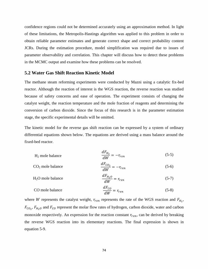
74
confidence regions could not be determined accurately using an approximation method. In light
of these limitations, the Metropolis-Hastings algorithm was applied to this problem in order to
obtain reliable parameter estimates and generate correct shape and correct probability content
JCRs. During the estimation procedure, model simplification was required due to issues of
parameter observability and correlation. This chapter will discuss how to detect these problems
in the MCMC output and examine how these problems can be resolved.
5.2 Water Gas Shift Reaction Kinetic Model
The methane steam reforming experiments were conducted by Mazni using a catalytic fix-bed
reactor. Although the reaction of interest is the WGS reaction, the reverse reaction was studied
because of safety concerns and ease of operation. The experiment consists of changing the
catalyst weight, the reaction temperature and the mole fraction of reagents and determining the
conversion of carbon dioxide. Since the focus of this research is in the parameter estimation
stage, the specific experimental details will be omitted.
The kinetic model for the reverse gas shift reaction can be expressed by a system of ordinary
differential equations shown below. The equations are derived using a mass balance around the
fixed-bed reactor.
H2 mole balance
(5-5)
CO2 mole balance
(5-6)
H2O mole balance
(5-7)
CO mole balance
(5-8)
where represents the catalyst weight, represents the rate of the WGS reaction and ,
, and represent the molar flow rates of hydrogen, carbon dioxide, water and carbon
monoxide respectively. An expression for the reaction constant , can be derived by breaking
the reverse WGS reaction into its elementary reactions. The final expression is shown in
equation 5-9.

75
(5-9)
In the above equation, k, , KCO, KS, and represent parameters while Kp, is the
equilibrium constant for the overall reaction that can be calculated from Perry’s Handbook. The
lowercase k is used to represent a rate constant while the uppercase K is used to denote an
equilibrium constant.
In order to obtain parameter point estimates and generate joint confidence regions, the
measurement error from the experiment must be quantified. This was accomplished through
replicate runs, which provided a standard deviation of = 0.01198 for the conversion of carbon
dioxide in the catalytic reactor. Assuming that the error follows a normal distribution, the
likelihood function can now be developed. The rate and equilibrium constants at each
temperature can be estimated using the posterior distribution function given below:
(5-10)
In equation, 5-10, the term is the experimentally observed conversion of carbon dioxide
while
represents the conversion obtained from the model. Since the MCMC algorithm
necessitates the calculation of the posterior density, the value of
must be determined at
each MCMC iteration. This involves integrating equations 5-5 to 5-8 simultaneously up to the
catalyst weight. The integration will yield the CO2 flow rate out of the reactor, which can then be
used in determining the conversion of carbon dioxide in the reaction.
(5-11)
Rather than estimating the rate and equilibrium constants at each individual temperature, the
following two equations provide a relationship between the kinetic constants and the
temperature.
(5-12)

76
(5-13)
where is the rate constant at the reference temperature, is the equilibrium
constant at the reference temperature, is the activation energy and is the standard enthalpy
change for the reaction. Estimation of these parameters requires using the entire data set and
replacing the rate and equilibrium constants in equation 5-9 with equations 5-12 and 5-13. Note
that a reference temperature of 998K was used in the MCMC methodology since it represents the
midpoint value of the four temperatures.
5.3 Model Simplification
The proposed rate expression shown in equation 5-9 required significant simplification due to
observability issues. Observability problems are often encountered in non-linear models and
properly dealing with this issue is an essential part of the parameter estimation protocol.
Therefore this chapter will illustrate how to detect parameters that cannot be estimated accurately
when Marko Chain Monte Carlo techniques are applied.
5.3.1 Issue of Observability
First, consider what happens when one tries to estimate all the parameters in the kinetic model.
To simplify the regression methodology, the rate and equilibrium constants at a single
temperature of 1023K will be estimated. This entails determining values for k, , KCO, KS, and
KH2O. The following Markov chain time series plot was obtained after implementing the single
component Metropolis-Hastings algorithm. Note that only the time series for and KCO are
shown.

77
Figure 5-1: The MCMC time series for the parameters and KCO
Figure 5-1 shows poor convergence of the Markov chain to its stationary distribution since the
mean value of the samples varies throughout the time series. An acceptance rate higher than 70%
was also observed for the two parameters. To understand the reason for poor mixing in the
Markov chain, a sensitivity analysis was carried out. This analysis provides information on
whether or not parameters in the given model can be estimated under the current experimental
conditions.
One method of measuring the sensitivity of a parameter is to calculate and plot the gradient
(equation 5-14) as a function of the independent variable.
(5-14)
where represents the change in the response variable and is the perturbation in the
parameters.
The gradient values can therefore be determined by perturbing one of the parameters and
determining the corresponding change in the response variable. The gradient can be normalized
by dividing it by the standard deviation so that any bias present in the measurement error can be
removed. In addition, comparing the gradient values of different parameters might not be
0 200 400 600 800 1000-200
0
200K
CO
2
0 200 400 600 800 1000-0.5
0
0.5
MCMC Cycle
KC
O

78
adequate since parameter values can differ by several orders of magnitude. This can be rectified
by multiplying the gradient values by 10% of the parameter values (Polic et al., 2004).
This method does have one limitation in that the parameter values must be known prior to
calculating the gradient. Therefore, non-linear least squares method must be first applied to
generate initial parameter estimates. Even though prior parameter estimates are required,
gradient plots are still useful in providing valuable information about parameter observability.
The gradient plots can be generated at each individual temperature using equation 5-14. A
similar trend was observed for temperatures between 923K and1023K; therefore, for brevity,
only the gradient plots at a temperature of 1023K are shown (Figure 5-2). At temperatures
between 923K and1023K, the gradient values for parameters k, KS, and were found to be
several orders of magnitude higher than the gradient values for parameters and KCO.
Parameters with higher gradient values can be estimated with greater precision. Therefore the
sensitivity analysis seems to indicate that for temperatures between 923K and 1023K, only
parameters k, KS, and can be estimated accurately.

79
Figure 5-2: The gradient plots for parameters k, KS, , KCO, and as a function of the catalyst
weight using data points at 1023K.
0.015 0.02 0.025 0.03 0.0350.35
0.4
0.45
Catalyst Weight
Grad
ien
t o
f k
0.015 0.02 0.025 0.03 0.035-4.9
-4.85
-4.8
-4.75
-4.7x 10
-4
Catalyst Weight
Grad
ien
t o
f K
CO
2
0.015 0.02 0.025 0.03 0.035 0.040.45
0.5
0.55
0.6
0.65
Catalyst Weight
Grad
ien
t o
f K
s
0.015 0.02 0.025 0.03 0.035-2.1
-2
-1.9
-1.8
-1.7
-1.6x 10
-6
Catalyst Weight
Grad
ien
t o
f K
CO
0.015 0.02 0.025 0.03 0.035-0.65
-0.6
-0.55
-0.5
-0.45
Catalyst Weight
Gra
die
nt of K
H2
O

80
The parameters and KCO can be removed and the rate expression can be simplified as shown
in equation 5-15.
(5-15)
Based on the results from the sensitivity analysis, it appears that the poor mixing in the Markov
chain, that was visible in Figure 5-1, is related to parameter observability. Perturbing the
parameter KCO2 and KCO produced little change in the response variable. The poor sensitivity in
these parameters translates into a high transitional probability for the Markov chain due to the
fact that when the transition probability is calculated, the density at the current value will be
similar to the density at the proposed value. The high transitional probability could be the reason
for the high acceptance rate that was observed for parameters KCO2 and KCO. The results in this
case study illustrate how the issue of observability can be detected from examining the MCMC
output. A high acceptance rate that persists even after tuning the algorithm could be an indication
of poor observability in the parameters.
It should be noted that the parameters and KCO do become significant at 1073K as shown in
Figure 5-3. However, since these parameters were found to be negligible between the
temperatures of 923K to 1023K, their inclusion in the rate expression cannot be justified.
Figure 5-3: The gradient plots for parameters and KCO as a function of the catalyst weight
using data points at 1073K. These two parameters become observable at the highest temperature.
0.015 0.02 0.025 0.03 0.035-0.3
-0.28
-0.26
-0.24
-0.22
-0.2
Catalyst Weight
Grad
ien
t o
f K
CO
0.015 0.02 0.025 0.03 0.035-0.0195
-0.019
-0.0185
-0.018
-0.0175
Catalyst Weight
Grad
ien
t o
f K
CO
2

81
5.3.2 Issue of correlation between parameters
After the sensitivity analysis was conducted, the Metropolis-Hastings algorithm was applied
using the simplified rate expression given by equation 5-15. Once again, after analyzing the
MCMC output, it became evident that the Markov chain for parameters KS and was not
able to converge to the desired distribution. As shown in Figure 5-4, the sampled MCMC values
for these two parameters are not stationary. The Markov chain for the rate constant k, however,
appears to have converged since the mean is constant throughout the MCMC cycle. The
acceptance rates for KS and were around 80% further indicating a lack of convergence.
Figure 5-4: MCMC output values for parameters k, KS and at a temperature of 1073K.
Since the sensitivity analysis showed reasonably high gradient values for these parameters, we
know that observability is not the issue. Rather, the convergence problem lies in the high degree
of correlation between these two parameters. Closer inspection of Figure 5-4 reveals that the
values for KS and move up and down simultaneously. This correlation is a consequence of
the rate expression shown in equation 5-15, where KS and appear as a ratio. Both
parameters cannot be estimated together because there are multiple values for each parameter
that will result in the same ratio. Therefore the model needs to be reparameterized and the ratio
of the two equilibrium constants (written as KL) must be estimated.
0 1 2 3 4 5 6 7
x 104
1
1.2
1.4
k
0 1 2 3 4 5 6 7
x 104
0
0.1
0.2
Ks
0 1 2 3 4 5 6 7
x 104
0
2
4
MCMC Cycle
KH
2O

82
(5-16)
Although reparameterization of the model involved removing the parameter from second
term in the denominator, the parameter still appears in the third term. Therefore, it is important to
verify that the parameter , is still observable by conducting a sensitivity analysis. The
generated gradient plots are shown in the Figure 5-5.
Figure 5-5: The gradient plots for parameters k, KL and KH2O as a function of the catalyst weight
using data points at 1023K. The reparameterized model shown in equation 5-15 was applied.
The gradient values obtained from these plots suggest that the parameter is no longer
observable. Since the parameter could not be estimated under the current experimental
conditions, it was dropped and the final simplified model is shown below:
0.015 0.02 0.025 0.03 0.035
0.35
0.4
0.45
Catalyst Weight
Para
mete
r k
0.015 0.02 0.025 0.03 0.035-0.65
-0.6
-0.55
-0.5
-0.45
Catalyst Weight
Para
mete
r K
L
0.015 0.02 0.025 0.03 0.035-2.4
-2.2
-2
-1.8
-1.6x 10
-4
Catalyst Weight
Para
mete
r K
H2
O

83
(5-17)
The results from this section demonstrate how to diagnose observability and correlation issues
properly through analysis of the MCMC output. Observability limitations are often characterized
by high acceptance rates and non-stationary Markov chain behaviour. These conditions are also
inherent when there is correlation between two parameters. Correlation must therefore, be
detected by inspecting the Markov chain time series in order to observe whether the parameters
are moving up and down simultaneously. Once it has been established which parameters can be
estimated, the MCMC protocol outlined in Chapter 3 can be implemented.
5.4 Reverse Water-Gas Shift Reaction Results
5.4.1 Point Estimate and Joint Confidence Regions
Although the model simplification procedure considered the rate and equilibrium constants at
each individual temperature, it is more convenient to estimate the activation energy, standard
enthalpy of change and reference temperature parameters. These parameters can then be applied
to calculate rate and equilibrium constants at any temperature. The simplified model shown in
equation 5-17 can be used, only this time, the values for k and KL can be expressed in term of the
, , , and .
(5-18)
The Metropolis-Hastings algorithm was executed for 100,000 cycles in order to get a good
estimate of the sample mean. The parameters , and were sampled as one block while the
reference parameters were sampled in another block. The initial guess for the MCMC algorithm
was based on the optimization results that were obtained by Mazni. Analysis of the MCMC
output yielded acceptance rates of 22% for the energy parameters and 38% for the reference
temperature constants. These acceptance rates are close to the ideal acceptance rate of 23% and

84
therefore it appears that for the simplified model, the Markov chain has converged to the target
distribution.
Parameter point estimates and the standard deviation for all four parameters are also shown in
Table 5-1. The estimates were obtained by taking the mean of the samples obtained in MCMC
analysis and the error was quantified using the standard deviation of the samples.
Table 5-1: The parameters estimates and their respective error obtained from MCMC analysis
using all four temperature points. A midpoint temperature value of T= 998K was used as the
reference temperature
Parameters Estimate Standard
Deviation
(molmin-1
g-1
atm-1
) 0.3466 0.0279
33.3474 2.9818
(J/mol) 106830 12341
(J/mol) -63661 13386
The MCMC samples can be used to generate joint confidence region with correct shape and
correct probability content (Figures 5-6 and 5-7). Note that the slightly ragged lines and the small
islands shown on the joint confidence region are an artifact of the contouring program.

85
Figure 5-6: A 95% joint confidence region for parameters and . The plus sign
in the middle of the confidence region represents the sample mean.
Figure 5-7: A 95% joint confidence region for parameters , and . The plus sign in the
middle of the confidence region represents the sample mean.
k (Tref)
KL (
Tre
f)
0.3 0.32 0.34 0.36 0.38 0.4 0.42 0.44
30
35
40
Ek
Delt
aH
KL
0.6 0.7 0.8 0.9 1 1.1 1.2 1.3 1.4
x 105
-9
-8
-7
-6
-5
-4
x 104

86
This case study once again exemplifies the advantage of applying MCMC techniques in non-
linear model. While the optimization algorithm was found to depend highly on the initial guess,
MCMC methods provided reliable parameter estimates. In addition, accurate joint confidence
regions were also attained as shown in Figures 5-6 and 5-7. Therefore, the results further
strengths the argument that Markov Chain Monte Carlo represents a robust and efficient
approach to parameter estimation in non-linear models.
5.4.2 Model Validation
Once the parameters are estimated, graphical diagnostic checks can be implemented to verify
that the model is able to accurately fit the data. First, the residuals were plotted at each
experimental run. Ideally, the residual values should be randomly scattered around a mean of
zero. Any visible trends in these plots indicate that the model was not able to effectively capture
all of the uncertainty.
Figure 5-8: A plot of the residuals as a function of the experimental number
Examination of the residual plot reveals that the residuals are randomly distributed about zero
with no visible trend. This indicates that the simplified rate expression is able to model the data
accurately. To examine how the predicted values compare with the experimental observations,
consider Figure 5-9 below.
0 10 20 30 40 50 60 70 80-0.1
-0.05
0
0.05
0.1
Experimental Number
Resid
ual

87
Figure 5-9: A plot of predicted values compared with experimentally observed values
The plot shows that the predicted values using the parameter estimates give similar results when
compared to the experimental data. Therefore, it is evident that the model is able to provide an
accurate prediction of the observed experimental data. It is hoped that the finding from this work
can be used to further advance the research in solid oxide fuel cells.
5.5 Summary
The following conclusions can be made from the Solid Oxide Fuel Cell case study:
1. Non-stationary behaviour of a Markov chain coupled with a high acceptance rate can be
an indication of poor parameter observability. In these situations, gradient plots must be
generated and the appropriate parameters must be removed.
2. Correlation between the parameters can be diagnosed by analyzing the Markov chain
time series and visually determining whether the two time series follow the same trend.
Reparameterization of the model might be required before a regression approach can be
implemented.
0 20 40 60 80 100 1200
0.2
0.4
0.6
0.8
Experiment Number
CO
2 C
onvers
ion
Predicted Values
Experimental Observations

88
3. Parameter point estimates and exact JCRs can be attained using the MCMC
methodology. The relative simplicity of the estimation methodology as well as the
reliability of the parameter estimates illustrates why applying MCMC methods in non-
linear models is advantageous.
4. The predicted model output was shown to closely resemble the experimentally observed
values. Therefore the parameters estimated in this research can be applied in future Solid
Oxide Fuel Cell studies.

89
Chapter 6: Parameter Estimation in Waterloo Polymer
Simulator Program
6. 1 Introduction
The Waterloo Polymer Simulator Program (Watpoly for short), is a comprehensive mechanistic
reactor model for multi-component polymerization. It has been developed in the Department of
Chemical Engineering at the University of Waterloo, by the group of Professor A. Penlidis’ (Gao
and Penlidis, 1996, 1998 and 2000, and Jung, 2008). The polymerization simulation can be
carried out in bulk or in solution and the reactor configuration can be batch, semi-batch or
continuous. In addition to the polymerization model, the Watpoly program also includes a
database of polymerization physico-chemical properties and kinetic parameters. The aim of this
work is to estimate a few select parameters in the database using the Markov Chain Monte Carlo
approach.
In the parameter estimation protocol, the first step is to obtain polymerization data. Comparison
of the model prediction results with experimental findings has shown that the Watpoly program
has strong prediction capabilities (Gao and Penlidis, 1996, 1998 and 2000, and Jung, 2008).
Therefore, the experimental data used in this case study will be simulated using the program. An
appropriate error term will be added to each of the response variables in order to replicate a
laboratory experiment. After a sufficient number of experiments have been conducted, the
Watpoly program can be applied again, this time in conjunction with the MCMC algorithm.
Parameter point estimates and joint confidence regions can then be presented.
Parameter estimation in the Watpoly program was previously explored by Polic et al. (2004). An
optimization algorithm was applied in determining parameter estimates while exact shape JCRs
were generated to capture the parameter uncertainty. Implementation of the optimization
algorithm however, proved to be difficult since local optima were encountered during the
estimation procedure. In addition, the confidence regions obtained using the exact shape
approximation technique failed to capture the parameter uncertainty adequately. Therefore the
central motivation behind this chapter is to determine whether these limitations can be rectified
using an MCMC approach. This chapter will provide a brief overview of the polymerization

90
models, discuss the polymerization conditions and finally compare the results from Polic’s work
with the MCMC results.
6. 2 Waterloo Polymer Simulator Theory
Explanation of all the equations utilized in the Watpoly program is beyond the scope of this
thesis. Therefore, the following section will explore only the important steps and equations used
in the simulator. In addition, modeling equations that pertain specifically to the parameters and
response variables used in this case study will be highlighted. For a more comprehensive
understanding and description of the Watpoly program, refer to Jung (2008).
6.2.1 Polymerization Reaction Kinetics
Free radical polymerization reactions can be divided into three main steps: initiation, propagation
and termination. Each of these steps will be explained briefly and the important equations will be
presented.
Initiation:
The initiation step can be split into two separate reactions. First, the initiator decomposed to
form two primary radical fragments (Equation 6-1).
(6-1)
These primary radicals can then react with the monomer , to form a radical that is the
length of one monomer (Equation 6-2). The notation i is in reference to the monomer type at the
end of the chain, while the number 1 refers to the length of the chain. This same notation will be
applied in subsequent equations.
(6-2)
Using equation 6-1, the rate of initiation can be written as:
(6-3)
where is the initiator efficiency, is the rate constant of initiator decomposition and [I] is
the concentration of initiator. The equation above can only be applied in the case of a

91
homopolymerization. When multiple monomers are being used, the pseudo decomposition rate
constant and pseudo initiator efficiency must be utilized.
Propagation
In modeling the propagation step, the “terminal” model will be considered. This model assumes
that the reaction rate is only influenced by the monomer unit at the end of the propagating chain.
The polymer grows by the addition of monomer units to the end of the polymer chain as shown
below:
(6-4)
The rate of polymerization is one of the response variables used in the case study and it can be
calculated using the following equation:
(6-5)
where [M] is the total concentration of monomer, kp is the propagation rate constant and is
the total concentration of radicals. Note that the pseudo propagation rate constant must be used if
more than one monomer species is present. The total radical concentration represents another
unknown whose equation can be determined by applying the steady-state hypothesis.
(6-6)
Termination
There are two main termination reactions. The radical chain can either combine to form a single
new dead polymer chain (Equation 6-7) or it can form two different polymer chains (Equation 6-
8).
(6-7)
(6-8)

92
The termination rate expression can be derived for a homopolymer system based on the above
equations.
(6-9)
Although equations 6-7 and 6-8 represent the major sources of termination, a polymer chain can
also be formed by transfer of the radical to the monomer, chain transfer agent, solvent or
inhibitor. For the purposes of this work, these radical transfer equations will be omitted.
6.2.2 Mole Balances
Modeling of any polymerization process requires mole balance around the monomer (equation 6-
10) and polymer species (equation 6-11), as shown below:
(6-10)
(6-11)
where, Ni represents moles of species i, Fi,in is the molar flow rate into the reactor, Rpi is the rate
of consumption of monomer and VT is the volume of the reaction mixture. The index i is in
reference to monomer type. The above equation can be easily simplified for a batch process by
setting the inflow rate to zero. The conversion of the polymerization, one of the response
variables used in this case study, can then be estimated using the molar balances and equation 6-
12. Examination of the plot of conversion as a function of time can yield valuable information
about how quickly the reaction progresses.
(6-12)
6.2.3 Diffusion-control kinetics
Diffusional limitations can occur in a polymerization reaction, especially at middle to high
conversion levels. In order to address this issue, the free-volume approach has been applied in
the Watpoly program. The equation for the free volume of the monomer is given by:

93
(6-13)
where is the free volume of monomer at the glass transition temperature, is the thermal
expansion coefficient, is the glass transition temperature of the monomer, is the reaction
temperature, is the volume of the monomer and is the total reaction volume. Note that
is a parameter that will be estimated in this case study.
The propagation reaction can become diffusion-controlled if the total free volume is less than a
critical free volume. Therefore the following relationship can be applied to take this effect into
account.
(6-14)
where parameters and correspond to the free volume and critical free volume
respectively, while is the glass-transition effect model parameter. Note that will be
one of the parameters estimated in this case study. Although the equations have been omitted
from this report, the Watpoly program considers diffusion limitations in the termination, transfer
reaction and initiation efficiency rate constants.
6.2.4 Molecular Weight
Since the weight and number average molecular weights are two of the responses used in this
case study, a brief overview on how to calculate these parameters will be provided below. The
zeroth, first and second moments of the polymer distribution for linear chains are shown below
(Polic et al., 2004):
(6-15)
(6-16)
(6-17)

94
where
(6-18)
(6-19)
The cumulative number and weight average molecular weights can then be determined by:
(6-20)
(6-21)
6. 3 Conditions for the Parameter Estimation Protocol
Recall that the primary objective of this chapter is to determine whether the limitations
encountered in Polic’s thesis can be resolved using an MCMC approach. Therefore, the
parameters and response variables used in this case study will be identical to those reported in
Polic’s thesis. The experimental conditions for the Watpoly simulation were changed slightly
from Polic’s work due to computational issues. The following section will discuss these CPU
time limitations and provide a general overview of the conditions used in the entire parameter
estimation procedure.
6.3.1 Parameters and Response Variables
The MCMC algorithm will be applied to the homopolymerization of styrene in order to estimate
three parameters within the Watpoly model. These three parameters, which have been described
briefly in the theory section, are summarized below:
1. αm = The thermal expansion coefficient for the monomer (free volume units/K)
2. BBm = Rate of decrease of kP (L/mol min per free volume unit)
3. Tgp = Glass transition temperature of the polymer (K)

95
The response variables used in estimating these three parameters are shown in Table 6-1. Note
that the error terms in Table 6-1 are based on the values reported by Polic (2001). The error
values have been corrected accordingly for the decrease in conversion (Penlidis, 2013).
Table 6-1: The response variables with the corresponding units and error applied in this case
study.
Response Units Error
Conversion ----- 0.025
Number Average
Molecular Weight (Mn) g/mol 4000
Weight Average
Molecular Weight (Mw) g/mol 4000
Rate of Polymerization mol/L/min 0.001
Radical Concentration mol/L 25%
6.3.2 Operating Conditions
Once the parameters and response variables are selected, the operating conditions for the
polymerization must be determined. The homopolymerization of styrene will be carried out
isothermally at a temperature of 65ºC. Since the temperature is constant, the only independent
variable is the reaction time. Plotting the conversion as a function of time can offer significant
insights into how quickly the reaction is progressing. Consider Figure 6-1, where the solid line is
used to represent the conversion curve obtained by Polic (2001). The conversion only starts to
plateau after 950 minutes. A longer reaction time will result in a more computationally intensive
MCMC algorithm since the numerical integration algorithm needs to be carried out for a much
longer time. Therefore the rate of polymerization was increased in our case study (conversion
curve shown by the dashed lines) by increasing the initiator concentration of AIBN to 0.28
mol/L.

96
Figure 6-1: The plot of conversion as a function of time for the homopolymerization of styrene at
65ºC
Examination of Figure 6-1 reveals that between 280 minutes and 330 minutes, the conversion for
the dashed curve rises sharply before plateauing. This steep increase can be attributed to an effect
known as auto-acceleration. Auto-acceleration occurs at a conversion level when an increase in
the reaction viscosity hinders the termination of the radical chains. This increases radical
concentration leading to the increase in the reaction rate depicted in Figure 6-1. It should be
noted that since both curves follow the same trend, comparison of the results from Polic’s work
with the results from the current work can be justified.
Ideally, experimental designs such as the D-optimality criterion should be applied in selecting
the optimal experimental conditions. However, since the focus of this research is in the
parameter estimation stage, the experimental runs will be chosen based on simple gradient plots.
Although gradient plots can be generated for all five responses, for the sake of brevity, only the
gradient values from the conversion response will be presented in this case study. The plots for
parameters αm and BBm are shown in Figures 6-2 and 6-3. The gradient plot for Tgp was omitted
since the gradient plot produced a similar trend as the gradient for parameter αm.
0 200 400 600 800 10000
0.2
0.4
0.6
0.8
1
Time (min.)
Convers
ion
Conversion Curve: Polic
Conversion Curve: Present Work
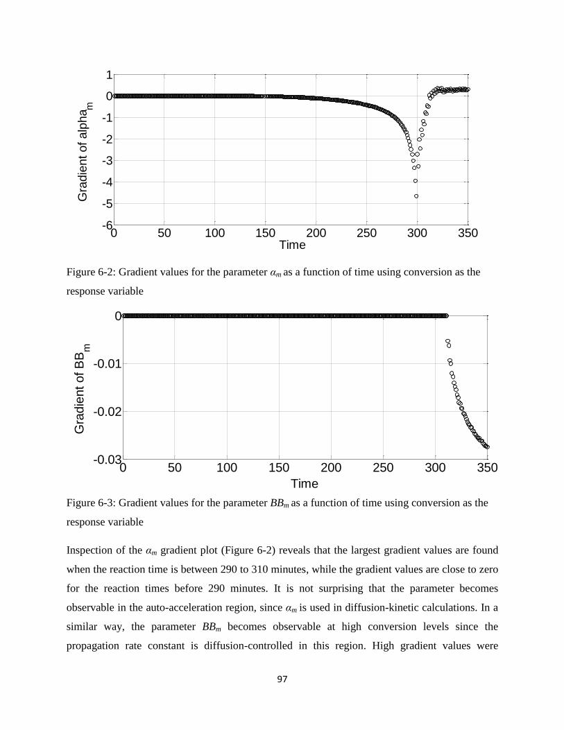
97
Figure 6-2: Gradient values for the parameter αm as a function of time using conversion as the
response variable
Figure 6-3: Gradient values for the parameter BBm as a function of time using conversion as the
response variable
Inspection of the αm gradient plot (Figure 6-2) reveals that the largest gradient values are found
when the reaction time is between 290 to 310 minutes, while the gradient values are close to zero
for the reaction times before 290 minutes. It is not surprising that the parameter becomes
observable in the auto-acceleration region, since αm is used in diffusion-kinetic calculations. In a
similar way, the parameter BBm becomes observable at high conversion levels since the
propagation rate constant is diffusion-controlled in this region. High gradient values were
0 50 100 150 200 250 300 350-6
-5
-4
-3
-2
-1
0
1
Time
Gra
die
nt of alp
ha
m
0 50 100 150 200 250 300 350-0.03
-0.02
-0.01
0
Time
Gra
die
nt of B
Bm

98
observed for parameter BBm after a reaction time of 310 minutes. Since both parameters become
observable at different regions in the conversion plot (αm becomes observable between 290 to
310 minutes, while BBm can be estimated using reaction time after 310 minutes), the two time
intervals can be combined as shown in Table 6-2. Each interval was divided into 10 reaction
times.
Table 6-2: The reaction times when each parameter becomes observable
Time
Parameter αm 290, 292, 294, 296, 298, 300, 302, 304, 306, 308,
Parameter BBm 316, 318, 320, 322, 324, 326, 328, 330, 332, 334
6.3.3 Experimental Simulation
Once the parameters, response variables and experimental conditions have been established, the
experimental data can be simulated. First the error terms for each response variable can be
generated using the error magnitudes shown in Table 6-1 and by assuming that the error follows
a normal distribution. Next the polymerization conditions described in section 6.3.2 and the
Watpoly program can be used to determine the true values. The measurements can then be
simulated by combining the true values from the Watpoly program with the error terms as shown
below:
(6-22)
where i is the response, u is the experimental trial, yui is the simulated measurement for the ith
response and the uth
trial, is the true value obtained from the Watpoly program and
is the measurement error for the ith
response and at the uth
trial.

99
Table 6-3: The simulated experimental data that was used in this case study
Run Time
(min) Conversion
Number
Average
Molecular
Weight
(g/mol)
Weight
Average
Molecular
Weight
(g/mol)
Polymerization
Rate
(mol/L/min)
Radical
Concentrat
ion (mol/L
1 290 0.777 1.59E+04 3.10E+04 2.30E-06 6.28E-02
2 292 0.772 2.23E+04 2.74E+04 2.00E-06 7.17E-02
3 294 0.798 1.96E+04 3.25E+04 4.59E-06 8.62E-02
4 296 0.845 2.04E+04 3.28E+04 6.26E-06 1.13E-01
5 298 0.914 2.15E+04 3.79E+04 3.16E-06 8.49E-02
6 300 0.858 1.87E+04 4.00E+04 3.60E-06 6.88E-02
7 302 0.857 1.96E+04 4.81E+04 2.89E-06 5.67E-02
8 304 0.897 2.07E+04 5.87E+04 3.14E-06 4.42E-02
9 306 0.869 1.84E+04 6.47E+04 2.82E-06 3.13E-02
10 308 0.882 2.41E+04 6.98E+04 2.12E-06 1.72E-02
11 316 0.906 2.21E+04 7.57E+04 1.68E-06 1.48E-03
12 318 0.883 1.86E+04 7.53E+04 2.49E-06 1.78E-03
13 320 0.877 2.23E+04 7.60E+04 3.45E-06 1.87E-03
14 322 0.889 2.17E+04 7.62E+04 2.26E-06 2.06E-03
15 324 0.920 2.01E+04 7.43E+04 3.48E-06 3.29E-04
16 326 0.890 2.07E+04 7.38E+04 5.31E-07 1.10E-03
17 328 0.885 1.85E+04 7.43E+04 2.54E-06 1.08E-03
18 330 0.961 2.00E+04 7.58E+04 2.44E-06 3.95E-04
19 332 0.879 2.10E+04 7.79E+04 2.29E-06 1.49E-03
20 334 0.872 2.34E+04 8.01E+04 2.09E-06 1.13E-03
6. 4 Results
The Metropolis-Hastings algorithm was applied to the simulated experimental data shown in
Table 6-3 in order to estimate the parameter values for αm, BBm and Tgp. All three parameters
were sampled as one block because the algorithm is computationally intensive. Since the
implementation steps for a multiresponse model have already been described in the triad fraction

100
case study, for the sake of conciseness, these steps will be omitted here. The only difference in
these two case studies lies in how the predicted response variables are calculated. In this case
study, the Watpoly program was used in determining the predicted response variables. Finally,
the tuning procedure described in Chapter 3 was implemented to obtain a fully converged
Markov chain.
6.4.1 Parameter Point Estimates Results
Due to the long CPU times, the MH algorithm could only be executed for 72,000 cycles. The
MCMC output for the three parameters is shown below.
Figure 6-4: The MCMC output values for parameters αm, BBm, and Tgp
The stationary behavior of the Markov chain time series signifies convergence of the Markov
chain to its stationary distribution. In addition, an acceptance rate of 22% was achieved
providing further evidence that the Markov chain has fully converged. Taking the average of the
samples shown in Figure 6-4, parameter values for αm, BBm, and Tgp were estimated to be
9.9968e-004 free volume units/K, 0.9829 L/mol min per free volume unit, and 377.97º K
respectively. Note that all the samples were used in calculating the average since a burn-in period
is not observed for the times series shown above.
Previous studies have shown that the actual sum of squares surface for this particular case study
contains numerous local optima. Consider Table 6-4, which shows the optimization results
0 1 2 3 4 5 6 7
x 104
0.99
1
1.01
x 10-3
Alp
ha
m
0 1 2 3 4 5 6 7
x 104
0.5
1
1.5
BB
m
0 1 2 3 4 5 6 7
x 104
377
378
379
MCMC Cycle
Tgp

101
obtained by Polic (2001) using different starting values. The final parameter estimate was found
to depend on where the optimization algorithm was started. Polic argued that the reason for
obtaining different parameter estimates is due to the presence of local optima.
Table 6-4: The results obtained when an optimization algorithm was applied using different
starting values (Polic, 2001).
Parameter Initial Values Final Values
Simulation 1
αm (free volume units/K) 0.001 0.001001
BBm (L/mol min per free volume unit) 1.00 1.02
Tgp (º K) 383.15 383.49
Simulation 2
αm (free volume units/K) 0.0015 0.00102
BBm (L/mol min per free volume unit) 1.5 1.147
Tgp (º K) 400 390.23
Simulation 3
αm (free volume units/K) 0.001 0.00102
BBm (L/mol min per free volume unit) 1.5 1.542
Tgp (º K) 390 396.94
Simulation 4
αm (free volume units/K) 0.0015 0.00107
BBm (L/mol min per free volume unit) 0.5 0.536
Tgp (º K) 350 418.71
The stationary behavior of the Markov chain, depicted in Figure 6-4, indicates that despite the
occurrence of local optima in the sum of squares surface, the MCMC algorithm can still provide
reliable parameter estimates once the chain enters its stationary distribution. However, it will be
interesting to observe whether or not the Markov chain will move towards the mean value when
different initial guesses are used. That is, will the presence of local optima influence the
convergence of the Markov chain when the chain is started away from its mean value? To
answer this question, initial guesses above and below the actual parameter values were used. The
starting values of 1.05 x 10⁻³
free volume units/K and 9.5 x 10⁻⁴
free volume units/K were used
for αm, 0.5 L/mol min per free volume unit and 2 L/mol min per free volume unit for BBM and
370 º K and 390 º K for Tgp. The Markov chain for each parameter is shown in the Figures 6-5 to
6-7.

102
Figure 6-5: The MCMC output values for parameter αm when an initial guess of 1.05 x 10⁻³
free
volume units/K (top plot) and an initial guess of 9.5 x 10⁻⁴
free volume units/K (bottom plot)
were used.
Figure 6-6: The MCMC output values for parameter BBm L/mol min per free volume unit when
an initial guess of 0.5 L/mol min per free volume unit (top plot) and an initial guess of 2 (bottom
plot) were used.
0 100 200 300 400 5000.9
1
1.1x 10
-3
MCMC Cycle
Alp
ha
m
0 500 1000 1500 20000.9
1
1.1x 10
-3A
lpha
m
0 50 100 150 200 2500.5
1
1.5
BB
m
0 50 100 1500
2
4
MCMC Cycle
BB
m

103
Figure 6-7: The MCMC output values for parameter Tgp when an initial guess of 370 º K (top
plot) and an initial guess of 390 º K (bottom plot) were used.
Figures 6-5 to 6-7 show that regardless of where the Markov chain is started, it quickly moves
towards its mean value. The speed at which the chain enters its stationary distribution is found to
vary from parameter to parameter. When 370 º K is used as an initial guess for Tgp , the chain
reaches its mean value of 380 º K in only 70 cycles. On the other hand, the Markov chain for
parameter αm requires 2300 cycles for reaching its mean value of 1x10⁻³
. Although the length of
the burn-in period was found to vary among the parameters, the Markov chain for all the
parameters reached its mean value in a reasonable time. Therefore, the results presented above
illustrate the advantage of applying MCMC methods in non-linear models. While the
optimization algorithm was limited by the presence of local optima, MCMC techniques produced
accurate parameter estimates.
6.4.2 Joint Confidence Regions
Recall that in Chapter 4, the exact shape JCRs were found to be in fairly good agreement with
the results obtained from the MCMC methodology. It will be interesting to see if this
approximation method is still accurate in this particular case study, where a more complex non-
linear model is being applied. To provide a comparison, joint confidence regions were
constructed for parameters αm and BBm and for parameters αm and Tgp.
0 20 40 60 80 100 120370
380
390
MCMC Cycle
Tgp
0 10 20 30 40 50 60 70360
370
380T
gp

104
Figure 6-8: Joint confidence region for parameters αm and BBm obtained using the exact shape
approximation (Polic, 2001). The star represents the parameter point estimate.
Figure 6-9: Joint confidence region for parameters αm and BBm obtained using the MCMC
algorithm. The plus sign represents the parameter point estimate.
alpham
BB
m
9.92 9.94 9.96 9.98 10 10.02 10.04
x 10-4
0.7
0.8
0.9
1
1.1
1.2
1.3

105
Figure 6-10: Joint confidence region for parameters αm and Tgp obtained using the exact shape
approximation (Polic, 2001). The star represents the parameter point estimate.
Figure 6-11: Joint confidence region for parameters αm and Tgp obtained using the MCMC
algorithm. The plus sign represents the parameter point estimate.
Let us first consider the joint confidence region for parameters αm and BBm. Comparison of
Figure 6-8 and 6-9 reveals two major problems with the exact shape JCRs. First, the
alpham
Tgp
9.92 9.94 9.96 9.98 10 10.02 10.04
x 10-4
377.4
377.6
377.8
378
378.2
378.4

106
approximation JCR (Figure 6-8) does not come to a close at large BBm values. As a result, a
significant portion of the αm and BBm is being considered when it should be rejected based on a
95% confidence level. In addition, the approximation method was not able to adequately capture
the shape of the confidence region. Similar problems are encountered when the JCRs between αm
and Tgp are compared. Figures 6-10 and 6-11 are similar in that they both indicate high
correlation between the two parameters. However, once again, the approximate JCR does not
come to a close at the top portion of Figure 6-10 resulting in an incorrect confidence region. The
results of this case study demonstrate the fact that even exact shape approximations might not be
adequate when complex non-linear models are being utilized. MCMC methods must be applied
in these situations in order to obtained precise results.
6. 5 Summary
The primary purpose of this case study was to determine whether or not MCMC techniques can
address some of the limitations encountered when classical regression approaches are used. The
results showed that even when local optima were present, reliable parameter point estimates can
be obtained. In addition, while the exact shape approximation yielded incorrect shape and
probability content JCRs, MCMC methods were found to provide accurate uncertainty regions.
Therefore, it can be concluded that when dealing with complex non-linear models, MCMC
techniques are the only viable option for parameter estimation.

107
Chapter 7: Computational Issues in Applying MCMC
Techniques
7. 1 Introduction and Motivation
Executing MCMC algorithms require a large computational effort, especially when differential
or implicit equations are involved. This computational cost could be one possible reason for the
limited application of MCMC techniques in chemical engineering problems. Therefore, in order
to motivate future research in this field, this chapter will briefly examine computation times for a
wide variety of models and provide guidlelines for reducing CPU time.
7. 2 Computation Time
In order to better understand the feasibility of implementing MCMC techniques in non-linear
models, a summary of the computational times for each model is provided in Table 7-1. The
algorithms were executed on a 2.13 GHz Intel Core 2 processor. The values in Table 7-1
represents the time that is required to complete 100,000 cycles. This is the minimum number of
cycles that is required in order to obtain reliable parameter estimates and produce smooth JCRs.
It should be noted that if the number of cycles is increased ten times, the time will also be
increased tenfold.
Using results presented in Table 7-1, the following conclusions can be made:
1. Computational time is not an issue when MCMC techniques are applied to explicit
analytical equations. The MCMC algorithms for the analytical BOD model and the
Mayo-Lewis model were completed in a much shorter time when compared to the other
non-linear models.
2. When MCMC methods are implemented in implicit equation models, the computational
time is found to increase significantly since each iteration requires the execution of a root
finding algorithm.
3. The largest CPU times were observed in the differential equation models. Recall that
solving these types of models involves numerical integration of the differential equation
at each MCMC cycle. Even small increases in computation time for one cycle can have a
drastic impact on the overall time.

108
4. It must be noted that there are significant differences in computational times among the
various differential equation models. These differences are based on the number of times
each differential equation is solved in one MCMC cycle. For the BOD problem, since
time is the only dependent variable, the differential equation only needs to be solved
twice per MCMC cycle (once to find the density of the current sample and once again to
find the density of the proposed sample). The direct numerical integration model
however, needs to be solved 32 times for each experimental run since each trial has a
different differential equation. Therefore the model structure as well as the number of
experimental runs has a large impact on how quickly the algorithm is executed.
The results presented above can provide a rough time scale for chemical engineers who are
interested in applying MCMC techniques to computationally intensive non-linear models.
7. 3 Methods for Reducing Computational Time
7.3.1 Serial Farming on Sharcnet
Running the MCMC algorithm on multiple processors can decrease the computational time
significantly. This can be accomplished using the SHARCNET computer cluster. SHARCNET is
a network of high performance computers that are available for researchers in Canada who need
to run computationally intensive jobs. There are two approaches that can be utilized in running
MCMC code on multiple CPUs. The first method involves creating Matlab code that can be run
in parallel on multiple processors. However, since parallelization of MCMC algorithm can be
quite challenging, this method will not be explored in this work. Some suggestions will be
provided in Section 8.2 on how this can be accomplished for future research. The second
technique involves using a process known as “serial farming”. Serial farming entails running the
same sequential code multiple times on different CPUs. It differs from parallel computing in that
there is no communication between the CPUs. The following five steps can be used to run serial
farming algorithms. This procedure will be illustrated using the direct numerical integration
model.
1. Run the MCMC algorithm for 3,000 - 5,000 cycles on the desktop CPU. This is to
determine whether or not the Markov chain is converging to its stationary distribution. If
convergence has not yet been achieved, use the tuning methodology provided in Chapter

109
3. Remove any observed burn-in period and take the average of the MCMC samples,
which will be the initial guess used in the serial farming approach.
2. Log on to SHARCNET and transfer all the required files to the computer cluster.
Compile the Matlab code to an executable file on Sharcnet so that it can be run multiple
times without a license. When using Matlab in carrying out the MCMC algorithm, it is
important to specifically assign the seed for the random number generator. Otherwise, all
the different MCMC chain will have the exact same values.
3. Determine the number of iterations and evenly divide these iterations among the different
CPUs. For the direction numerical integration example ten CPUs will be used and the
100,000 cycles will be divided into 10,000 cycles for each CPU.
4. Submit the ten serial jobs to the computer cluster using the specific documentation
provided by Sharcnet (Hu, 2013). The output for the direction numerical integration
example is shown in Figure 7-1. Note that since the burn-in period was removed in step
1, the ten MCMC chain are stationary at all times.
5. Generate one long chain by combining the ten smaller chains together. This is illustrated
in Figure 7-2. The long chain can now be used to obtain a more precise estimate of the
MCMC sample mean and smoother curves for the JCRs.
When using this serial farming approach with 10 CPUs, the direct integrated model was carried
out in only 0.8361 hours. This is an approximate decrease of 96% when compared to the results
from using 1 CPU. Therefore this approach represents a computationally efficient way to run
MCMC algorithms. The computational effort of running MCMC algorithm on 1 desktop
computer is compared with the time required to run the code on a computer cluster with 10 CPUs
in Table 7-1.
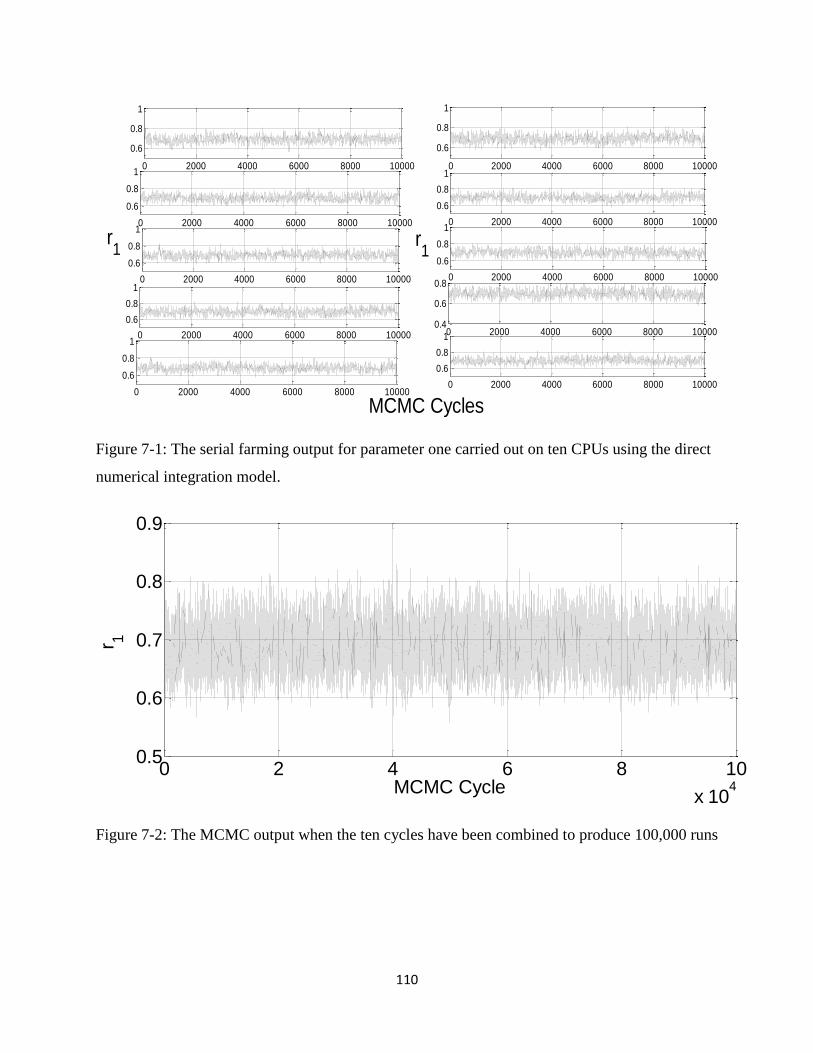
110
Figure 7-1: The serial farming output for parameter one carried out on ten CPUs using the direct
numerical integration model.
Figure 7-2: The MCMC output when the ten cycles have been combined to produce 100,000 runs
0 2000 4000 6000 8000 10000
0.6
0.8
1
0 2000 4000 6000 8000 10000
0.6
0.8
1
0 2000 4000 6000 8000 10000
0.6
0.8
1
0 2000 4000 6000 8000 10000
0.6
0.8
1
0 2000 4000 6000 8000 10000
0.6
0.8
1
0 2000 4000 6000 8000 10000
0.6
0.8
1
0 2000 4000 6000 8000 10000
0.6
0.8
1
0 2000 4000 6000 8000 100000.4
0.6
0.8
0 2000 4000 6000 8000 10000
0.6
0.8
1
0 2000 4000 6000 8000 10000
0.6
0.8
1
r1
r1
MCMC Cycles
0 2 4 6 8 10
x 104
0.5
0.6
0.7
0.8
0.9
MCMC Cycle
r 1

111
Table 7-1: The time required to complete 100,000 cycles for various non-linear models using
both desktop computer and a computer cluster with 10 CPUs.
Model Type of Model Required time with
1 CPU (hours)
Sharcnet time
with 10 CPUs
(hours)
Biological Oxygen
Demand
Analytical Explicit
Equation 0.011 0.019
Differential Equation 0.833 0.078
Mayo Lewis Model Analytical Equation 0.022 0.0056
Meyer Lowry Model Implicit Explicit Equation 10.8 0.333
Direct Numerical
Integration Differential Equation 21.3 0.836
Solid Oxide Fuel Cell System of Differential
Equations 153 2.85
Waterloo Polymer
Simulator
System of Differential
Equations 486 76
7.3.2 Other Guidelines for Reducing Computational Time
In addition to the serial farming approach, the following suggestions can help reduce the MCMC
computational time.
1. If Matlab is being used in executing the program, it is very important to pre-define the
size of all the large variables. For example, if a Matlab variable is being used to store all
the MCMC samples, then defining its size at the beginning of the MCMC algorithm can
drastically reduce the computational time. Another way to create an efficient Matlab
program is to replace loops with vector calculation whenever possible. Vectorizing the
code will result in a faster algorithm.
2. The computational time can also be decreased by using Matlab Coder to convert the
Matlab code to a C/C++ code. The code can be executed faster in the C/C++
environment.
3. The step size used in solving the differential equation has a drastic impact on how
quickly the algorithm runs. Although a small step size is better, using a step size too
small might not lead to any significant improvements in the final results. Therefore, it is

112
recommended that a preliminary study be carried out in order to determine the maximum
step size that can be used before accuracy in the parameter estimation procedure is
compromised.
4. Selection of the blocking scheme has a considerable impact on the computational time.
Each parameter or block of parameters requires the calculation of two density values (one
value for the candidate sample and the other for the current sample). This means that if
three parameters or blocks are used, then the computational intensity will increase three-
fold. Therefore sampling the parameters as one block is recommended in these situations.
It should be noted that it can be difficult to tune multiple parameters when only one
acceptance rate is produced. One method of tackling this issue is to select one parameter
and fix all the other parameters. The tuning of the proposal for that particular parameter
can now be carried out. Once a suitable acceptance rate is achieved, the same approach
can be applied to the other parameters. After the appropriate scaling values for each of
the parameters have been obtained, the parameters can now be estimated simultaneously.

113
Chapter 8: Conclusion and Recommended Future Steps
8.1 Concluding Remarks
This research work was motivated by the fact that although Markov Chain Monte Carlo methods
have been well established, it has not been applied extensively in chemical engineering literature.
Therefore, this work involved application of MCMC methodology in widely-used chemical
engineering models. In doing so, the three objectives that were described in Chapter 1 have been
addressed.
The first objective of this research was to discuss the implementation issues that can arise when
executing MCMC technique in various chemical engineering models .A summary of the results
is provided below:
An MCMC implementation procedure was presented in the biological oxygen demand
case study and each step was illustrated using specific BOD examples. The procedure
addressed the following issues: (1) how to select the proper MCMC algorithm, (2) the
influence of the starting value, (3) how to tune the scaling factors in the proposal
distribution, and (4) how to properly diagnosis whether or not the Markov chain has
converged.
The results from the BOD case study illustrates the importance of estimating the pure
error variance as a parameter instead of assigning it a value based on the mean squared
error. In addition, the results also show that the tuning of the proposal distribution can
become complicated if the posterior probability distribution has a heavy tail.
Parameter estimation of reactivity ratios involved analysis of various non-linear models.
The implementation procedure that was provided in Chapter 3 was then extended to
implicit equation models, differential equation models and multi-response models. Again
specific examples from the case study were used to exemplify these procedural steps.
The results from the solid oxide fuel cell case study show how parameter observability
and correlation can be detected from the analysis of the MCMC output. High acceptance
rates that are observed in conjunction with a non-stationary Markov chain could be an
indication of parameter observability. Parameter correlation, on the other hand, can be
identified when the parameters in the time series follow the same trend.

114
The MCMC implementation results as well as the MCMC protocol proposed in this
research can now be used as a guideline for chemical engineers who are interested in
applying these techniques in non-linear models.
After successful execution of the Markov Chain Monte Carlo techniques, the generated samples
were used to determine parameter estimates and produce joint confidence regions. Comparison
of these results with the findings obtained from classical regression approaches yielded the
following conclusions:
In the BOD case study, both approximation methods failed to accurately capture the
parameter uncertainty. The elliptical approximation overestimated the parameter
uncertainty while the exact shape region generated an open shaped joint confidence
region.
The elliptical approximation was found to overestimate the uncertainty in the Mayo-
Lewis model and underestimate the uncertainty in the Meyer-Lowry model. Although the
exact shape method was suitable for modeling parameter uncertainty in the Mayo-Lewis
model, it also produced incorrect probability content JCRs in the Meyer-Lowry model.
Therefore accurately capturing the parameter uncertainty in these models necessitates the
use of MCMC techniques.
The JCRs obtained from the triad fraction case study revealed a significant amount of
model-induced correlation. Individually estimating the parameter using MCMC methods
resulted in exact shape exact probability content JCRs with no correlation.
The findings from the solid oxide fuel cell case study illustrates the fact that reliable
parameter point estimates and accurate JCRs can only be obtained if a MCMC approach
is being utilized.
Finally, MCMC methods were applied in estimating a few select parameters in the
Watpoly simulator. Due to the presence of local optima, optimization methods yielded
inconsistent parameter estimates. In addition, open shaped JCRs were obtained when an
exact shape approximation was utilized. These limitations were remedied by applying
MCMC techniques.

115
The above results provide a strong argument for why MCMC techniques should be applied in all
non-linear models. For one, using an optimization algorithm might prove to be inadequate if
local optima are present. Second, the results from this research shows that approximate methods
for constructing JCRs can lead to erroneous results. Therefore MCMC techniques present an
accurate regression framework for determining parameter estimation in any non-linear models.
One of the major limitations of using MCMC techniques is its computational time. Although this
issue has been helped by the advances in computer technology and parallel programming, the
CPU time can still become an issue. Therefore the third objective of this study was to explore the
feasibility on implementing MCMC methods in various non-linear models. Based on the results,
the following conclusions can be drawn.
Computational time is not an issue when MCMC methods are applied for parameter
estimation in analytical models.
Computation times for various differential equations models have been provided in
Chapter 7. The computational cost of the algorithm is influenced by the blocking
scheme, the applied time step and the number of experimental runs.
A serial farming approach was presented as a means for reducing CPU time. In addition,
practical guidelines on how to generate computationally efficient code have been
provided.
To summarize, this research illustrated why MCMC methods are beneficial in parameter
estimation, addressed specific implementation issues, and provided guidelines for improving
computational speed. It is expected that the results from this work will initiate future
implementation of MCMC techniques in chemical engineering practices.
8.2 Future Work
8.2.1 Design of Experiments
Recall that in Chapter 6, the optimal polymerization conditions were determined based on the
gradient plot. A more appropriate technique is to select the optimal conditions using
experimental design. One approach that has widely being applied in the design of experiments is
the D-optimality criterion, where the hyper-volume of the linearized joint confidence region is

116
minimized. However, the criterion does have two major limitations: (1) it is only valid if the sum
of squares surface is linear in the neighborhood of the initial guess and (2) reliable results might
not be attained if local optima are present as shown by Polic (2001). Since Markov Chain Monte
Carlo methods can be used in generating the actual shape of the posterior distribution function,
more accurate results should be obtained. Therefore it is recommended that MCMC techniques
be applied in order to investigate whether or not these limitations can be addressed. In particular,
the BOD problem can be used as an initial case study. The currently used data set only consists
of seven data points that do not cover the entire time span. Therefore, MCMC methods can be
applied in determining additional data points for this problem.
8.2.2 Computational Feasibility Study
The computational limitations of solving differential equations were only examined very briefly
in this research. It is therefore recommended that a more comprehensive study be conducted on
how to decrease the computational time. This study should first examine how the integration step
size in the differential equations influences the MCMC results. Work on model simplification
and reduction can also be carried out in these differential equation models in order to create a
more efficient MCMC algorithm. Finally, the Matlab Coder software can be used in order to
generate C/C++ code. Research should be conducted to determine how much the computational
speed improves when the algorithm is executed in a C/C++ environment.
8.2.3 Parallel Computing
In order to run an MCMC algorithm in parallel using multiple processors, each of the MCMC
cycles must be independent from each other. Since Markov chains require the value of the
previous iteration in order to determine a new sample, executing the MCMC algorithms in
parallel can be challenging. There is currently a significant amount of research being conducted
in parallelizing MCMC code. One possible technique of parallelizing the MCMC algorithm has
been proposed by Campillo et al. (2009), who developed an algorithm that runs N multiple
interactive chains. In the proposed method, each individual chain is used to generate samples for
all other chains. Therefore, parallelizing the N interacting chains in each MCMC cycle will result
in a faster mixing in the Markov algorithm.

117
8.2.4 Adaptive Metropolis-Hastings
In the BOD example, poor convergence was observed when the Metropolis-Hastings algorithm
was applied to a posterior distribution with a heavy tail. Successfully mixing of the Markov
chain in these non-symmetric distributions requires a carefully designed proposal distribution.
This can be accomplished using an adaptive Metropolis-Hastings algorithm. Therefore further
research can be conducted on implementing the adaptive Metropolis-Hastings algorithm to
chemical engineering problems. In particular, the algorithm should be applied to highly non-
symmetric distributions similar to the one encounter in the BOD example.
8.2.5 Application of MCMC Methods using Experimental Data
With the exception of the solid oxide fuel cell study, the experimental data for all other case
studies were obtained from either computational simulation or literature sources. Therefore, the
next step is to now conduct actual laboratory experiments and apply MCMC methods to various
chemical engineering models. For example, the reactivity ratio in terpolymerization systems can
be estimating using this approach. Experimental design can be incorporated in the estimation
methodology in order to gain the maximum amount of information and replicate runs can be
carried out so that an accurate estimate of the pure error is known.
8.2.6 Application of MCMC Methods in Model Discrimination
This research work has focus solely on applying MCMC methods in regression analysis.
However, Markov Chain Monte Carlo can also be utilized in order to discriminate between rival
models. Although Masoumi et. al (2012) has proposed an efficient and reliable approach to
discriminating between candidate models, no experimental runs were carried out in their
research. Therefore the next step would be to apply MCMC methods in order to discriminate
between rival models using actual experimental data.
8.2.7 MCMC Software Program
One long term goal is to create a user-friendly program that can apply MCMC methods to any
non-linear model. The program will ask the user to input the experimental data, the model
structure, assumptions about the measurement error, prior knowledge and other MCMC related
options. It will then carry out the MCMC methodology, generating point estimates and joint
confidence regions. The software program should also have the following properties: (a) an

118
option to run parallel on a computer cluster (b) automatic tuning of the MCMC algorithm based
on the acceptance rates, and (c) be able to successfully diagnose convergence of the Markov
chain.

119
Appendix A: Experimental Data Used in the Solid Oxide Fuel
Cell Case Study
Table A-1: The experimental data obtained by Mazni Ismail in studying the solid oxide fuel cell
T (K) W.cat
(g)
Mol fraction CO2
Conversion
x,H2 x,CO2 x,CO x,H2O x,N2
1 1073 0.01522 0.59 0.08 0.00 0.00 0.33 0.40249
2 1073 0.01844 0.52 0.15 0.00 0.00 0.33 0.26430
3 1073 0.02327 0.42 0.25 0.00 0.00 0.33 0.17986
4 1073 0.02714 0.33 0.33 0.00 0.00 0.33 0.16635
5 1073 0.02549 0.40 0.35 0.00 0.00 0.25 0.18208
6 1073 0.02291 0.40 0.20 0.00 0.00 0.40 0.21635
7 1073 0.02119 0.40 0.10 0.00 0.00 0.50 0.29685
8 1073 0.01997 0.40 0.03 0.00 0.00 0.56 0.48553
9 1073 0.02655 0.32 0.28 0.00 0.00 0.40 0.17485
10 1073 0.03274 0.10 0.28 0.00 0.00 0.62 0.10270
11 1073 0.03004 0.20 0.28 0.00 0.00 0.52 0.08402
12 1073 0.03127 0.20 0.35 0.00 0.00 0.45 0.07707
13 1073 0.02907 0.15 0.15 0.00 0.00 0.70 0.16452
14 1073 0.02636 0.20 0.07 0.00 0.00 0.73 0.35823
15 1073 0.02759 0.20 0.14 0.00 0.00 0.66 0.20048
16 1073 0.02863 0.20 0.20 0.00 0.00 0.60 0.19211
17 1073 0.03232 0.07 0.20 0.00 0.00 0.73 0.11472
18 1073 0.03033 0.14 0.20 0.00 0.00 0.66 0.12673
19 1073 0.02634 0.28 0.20 0.00 0.00 0.52 0.21353
20 1073 0.02435 0.35 0.20 0.00 0.00 0.45 0.21242

120
21 1073 0.03179 0.07 0.19 0.02 0.00 0.71 0.10746
22 1073 0.02756 0.20 0.20 0.03 0.00 0.57 0.17919
23 1073 0.02649 0.20 0.20 0.07 0.00 0.53 0.22406
24 1073 0.02541 0.20 0.20 0.10 0.00 0.50 0.23685
25 1073 0.03033 0.14 0.20 0.00 0.03 0.66 0.09925
26 1073 0.02863 0.20 0.20 0.00 0.03 0.60 0.10399
27 1073 0.02634 0.28 0.20 0.00 0.03 0.52 0.14488
28 1073 0.02541 0.20 0.20 0.10 0.03 0.50 0.09734
29 1023 0.01522 0.59 0.08 0.00 0.00 0.33 0.31695
30 1023 0.01844 0.52 0.15 0.00 0.00 0.33 0.19234
31 1023 0.02327 0.42 0.25 0.00 0.00 0.33 0.12687
32 1023 0.02714 0.33 0.33 0.00 0.00 0.33 0.10596
33 1023 0.02549 0.40 0.35 0.00 0.00 0.25 0.12664
34 1023 0.02291 0.40 0.20 0.00 0.00 0.40 0.13078
35 1023 0.02119 0.40 0.10 0.00 0.00 0.50 0.18973
36 1023 0.01997 0.40 0.03 0.00 0.00 0.56 0.32052
37 1023 0.02655 0.32 0.28 0.00 0.00 0.40 0.11040
38 1023 0.03274 0.10 0.28 0.00 0.00 0.62 0.05519
39 1023 0.03004 0.20 0.28 0.00 0.00 0.52 0.04199
40 1023 0.03127 0.20 0.35 0.00 0.00 0.45 0.04017
41 1023 0.02907 0.15 0.15 0.00 0.00 0.70 0.08020
42 1023 0.02636 0.20 0.07 0.00 0.00 0.73 0.23165
43 1023 0.02759 0.20 0.14 0.00 0.00 0.66 0.12837
44 1023 0.02863 0.20 0.20 0.00 0.00 0.60 0.12875
45 1023 0.03232 0.07 0.20 0.00 0.00 0.73 0.07767
46 1023 0.03033 0.14 0.20 0.00 0.00 0.66 0.09868

121
47 1023 0.02634 0.28 0.20 0.00 0.00 0.52 0.15222
48 1023 0.02435 0.35 0.20 0.00 0.00 0.45 0.13029
49 1023 0.03179 0.07 0.19 0.02 0.00 0.71 0.07381
50 1023 0.02756 0.20 0.20 0.03 0.00 0.57 0.13083
51 1023 0.02649 0.20 0.20 0.07 0.00 0.53 0.16591
52 1023 0.02541 0.20 0.20 0.10 0.00 0.50 0.17752
53 1023 0.03033 0.14 0.20 0.00 0.03 0.66 0.05439
54 1023 0.02863 0.20 0.20 0.00 0.03 0.60 0.08111
55 1023 0.02634 0.28 0.20 0.00 0.03 0.52 0.08238
56 1023 0.02541 0.20 0.20 0.10 0.03 0.50 0.04841
57 973 0.01522 0.59 0.08 0.00 0.00 0.33 0.20966
58 973 0.01844 0.52 0.15 0.00 0.00 0.33 0.11552
59 973 0.02327 0.42 0.25 0.00 0.00 0.33 0.07293
60 973 0.02714 0.33 0.33 0.00 0.00 0.33 0.07712
61 973 0.02549 0.40 0.35 0.00 0.00 0.25 0.09566
62 973 0.02291 0.40 0.20 0.00 0.00 0.40 0.08155
63 973 0.02119 0.40 0.10 0.00 0.00 0.50 0.11915
64 973 0.01997 0.40 0.03 0.00 0.00 0.56 0.17482
65 973 0.02655 0.32 0.28 0.00 0.00 0.40 0.06813
66 973 0.03274 0.10 0.28 0.00 0.00 0.62 0.02729
67 973 0.03004 0.20 0.28 0.00 0.00 0.52 0.02166
68 973 0.03127 0.20 0.35 0.00 0.00 0.45 0.00828
69 973 0.02907 0.15 0.15 0.00 0.00 0.70 0.02603
70 973 0.02636 0.20 0.07 0.00 0.00 0.73 0.15403
71 973 0.02759 0.20 0.14 0.00 0.00 0.66 0.08306
72 973 0.02863 0.20 0.20 0.00 0.00 0.60 0.08916

122
73 973 0.03232 0.07 0.20 0.00 0.00 0.73 0.05488
74 973 0.03033 0.14 0.20 0.00 0.00 0.66 0.06659
75 973 0.02634 0.28 0.20 0.00 0.00 0.52 0.09928
76 973 0.02435 0.35 0.20 0.00 0.00 0.45 0.08450
77 973 0.03179 0.07 0.19 0.02 0.00 0.71 0.05442
78 973 0.02756 0.20 0.20 0.03 0.00 0.57 0.09210
79 973 0.02649 0.20 0.20 0.07 0.00 0.53 0.11808
80 973 0.02541 0.20 0.20 0.10 0.00 0.50 0.12794
81 973 0.03033 0.14 0.20 0.00 0.03 0.66 0.04438
82 973 0.02863 0.20 0.20 0.00 0.03 0.60 0.00000
83 973 0.02634 0.28 0.20 0.00 0.03 0.52 0.05803
84 973 0.02541 0.20 0.20 0.10 0.03 0.50 0.00665
85 923 0.01522 0.59 0.08 0.00 0.00 0.33 0.14287
86 923 0.01844 0.52 0.15 0.00 0.00 0.33 0.06950
87 923 0.02327 0.42 0.25 0.00 0.00 0.33 0.04224
88 923 0.02714 0.33 0.33 0.00 0.00 0.33 0.05738
89 923 0.02549 0.40 0.35 0.00 0.00 0.25 0.07775
90 923 0.02291 0.40 0.20 0.00 0.00 0.40 0.05520
91 923 0.02119 0.40 0.10 0.00 0.00 0.50 0.08075
92 923 0.01997 0.40 0.03 0.00 0.00 0.56 0.09817
93 923 0.02655 0.32 0.28 0.00 0.00 0.40 0.04251
94 923 0.03274 0.10 0.28 0.00 0.00 0.62 0.00976
95 923 0.03004 0.20 0.28 0.00 0.00 0.52 0.00753
96 923 0.03127 0.20 0.35 0.00 0.00 0.45 0.00000
97 923 0.02907 0.15 0.15 0.00 0.00 0.70 0.01855
98 923 0.02636 0.20 0.07 0.00 0.00 0.73 0.10955

123
99 923 0.02759 0.20 0.14 0.00 0.00 0.66 0.05670
100 923 0.02863 0.20 0.20 0.00 0.00 0.60 0.06155
101 923 0.03232 0.07 0.20 0.00 0.00 0.73 0.04119
102 923 0.03033 0.14 0.20 0.00 0.00 0.66 0.04835
103 923 0.02634 0.28 0.20 0.00 0.00 0.52 0.06777
104 923 0.02435 0.35 0.20 0.00 0.00 0.45 0.05456
105 923 0.03179 0.07 0.19 0.02 0.00 0.71 0.04223
106 923 0.02756 0.20 0.20 0.03 0.00 0.57 0.07197
107 923 0.02649 0.20 0.20 0.07 0.00 0.53 0.10124
108 923 0.02541 0.20 0.20 0.10 0.00 0.50 0.14036
109 923 0.03033 0.14 0.20 0.00 0.03 0.66 0.03446
110 923 0.02863 0.20 0.20 0.00 0.03 0.60 0.03764
111 923 0.02634 0.28 0.20 0.00 0.03 0.52 0.03051
112 923 0.02541 0.20 0.20 0.10 0.03 0.50 0.01488

124
Bibliography
Aerdts, A. M., de Haan, J. W., & German, A. L. (1993). Proton and carbon NMR spectra of
alternating and statistical styrene-methyl methacrylate copolymers
revisited. Marcomolecules, 26(8), 1965-1971.
Bard, Y. (1974). Nonlinear parameter estimation (Vol. 477). New York: Academic Press.
Bates, D. M., & Watts, D. G. (1988). Nonlinear Regression Analysis and Its Applications. New
York: Wiley.
Beale, E. L. (1960). Confidence Regions in Non-Linear Estimation. Journal of the Royal
Statistical Society. Series B (Methodological), 21(1), 41-88.
Box, G. E., & Draper, N. R. (1965). The Bayesian Estimation of Common Parameters from
Several Responses. Biometrika,52(3/4), 355 -365.
Box, G. P., & Tiao, G. C. (1992). Bayesian Inference in Statistical Analysis. New York: Wiley.
Brooks, S. (1998). Markov Chain Monte Carlo Method and Its Application. Journal of the Royal
Statistical Society Series D (The Statistician), 47(1).
Brooks, S. P., & Morgan, B. J. (1995). Optimization Using Simulated Annealing. Journal of the
Royal Statistical Society. Series D (The Statistician), 44(2), 241-257.
Burke, A. L., Duever, T. A., & Penlidis, A. (1997). Choosing the right model: Case studies on
the use of statistical modeldiscrimination experiments. The Canadian Journal of Chemical
Engineering, 75(2), 422-436.
Campillo, F., Rakotozafy, R., & Rossi, V. (2009). Parallel and interacting Markov chain Monte
Carlo algorithm. Mathematics and Computers in Simulation, 79, 3424-3433.
Conceição, E. T., & Portugal, A. G. (2012). Comparison of Two Robust Alternatives to the Box–
Draper Determinant Criterion in Multiresponse Kinetic Parameter Estimation. Industrial &
Engineering Chemistry Research, 53(3), 1118-1130.

125
Cowles, M. K., & Carlin, B. P. (1996). Markov Chain Monte Carlo Convergence Diagnostics: A
Comparative Review. Journal of the American Statistical Association, 91(434), 883-904
Chib, S., & Greenberg, E. (1995). Understanding the Metropolis-Hastings Algorithm. The
American Statistician, 49(4), 327-335.
Duever, T. A., Keeler, S. E., & Reilly, P. M. (1987). An application of the Error-in-Variables
Model—parameter estimation from Van Ness-type vapour-liquid equilibrium
experiments. Chemical Engineering Science, 42(3), 403-412.
Gao, J., & Penlidis, A. (1996). A Comprehensive Simulator/Database Package for Reviewing
Free-Radical Homopolymerizations. Journal of Macromolecular Science, Part C: Polymer
Reviews, 36(2), 199-404.
Gao, J., & Penlidis, A. (1998). A Comprehensive Simulator/Database Package for Reviewing
Free-Radical Copolymerizations. Journal of Macromolecular Science, Part C: Polymer
Reviews, 38(4), 651-780
Gao, J., & Penlidis, A. (2000). A comprehensive simulator/database package for bulk/solution
free-radical terpolymerizations.Macromolecular Chemistry and Physics, 201(11), 1176-1184.
Geman, S., & Geman, D. (1984). Stochastic Relaxation, Gibbs Distributions and the Bayesian
Restoration of Images. IEEE Transactions on Pattern Analysis and Machine Intelligence, 6(6),
721-741.
Geyer, C. (1992). Practical Markov Chain Monte Carlo. Statistical Science, 7(4), 473-483.
Gelman, A., & Rubin, D. B. (1992). Inference from Iterative Simulation Using Multiple
Sequences. Statistical Science, 7(4), 457-472.
Gelman, A., Roberts, G. O., & Gilks, W. R. (1996). Efficient Metropolis Jumping
Rules. Bayesian Statistics, 5, 599-607.
Gilks, W. R., Clayton, D. G., Spiegelhalter, D. J., Best, N. G., McNeil, A. J., Sharples, L. D., &
Kirby, A. J. (1993). Modelling Complexity: Applications of Gibbs Sampling in
Medicine. Journal of the Royal Statistical Society. Series B (Methodological), 55(1), 39-52.

126
Gilks, W. R., Richardson, S., & Spiegelhalter, D. J. (1996). Markov Chain Monte Carlo In
Practice. New York: Chapman-Hall.
Haario, H., Saksman, E., & Tamminen, J. (1999). Adaptive proposal distribution for random
walk Metropolis algorithm.Computational Statistics, 14(3), 375-396.
Haario, H., Saksman, E., & Tamminen, J. (2001). An adaptive Metropolis
algorithm. Bernoulli, 7(2), 223-242.
Hastings, W. K. (1970). Monte Carlo sampling methods using Markov Chains and their
applications. Biometrika, 57(1), 97-109.
Hu, J. (2013). Matlab documentation. In SHARCNET. Retrieved August 18, 2013, from
https://sharcnet.ca/help/index.php/MATLAB
Jarner, S. F., & Roberts, G. O. (2007). Convergence of Heavy-tailed Monte Carlo Markov Chain
Algorithms. Scandinavian Journal of Statistics, 34(4), 781-815.
Jeffreys, H. (1961). Theory of Probability (3rd ed.). Oxford: Clarendom Press.
Jitjareonchai, J. J. (2006). Implementation of Markov Chain Monte Carlo Techniques in
Parameter Estimation for Engineering Models. Ph.D thesis, University of Waterloo.
Jitjareonchai, J. J., Reilly, P. M., Burton, P. R., & Chambers, D. B. (2006). Parameter Estimation
in the Error-in-Variables Models Using the Gibbs Sampler. The Canadian Journal of Chemical
Engineering, 84(1), 125-138.
Jung, W. (2008). Mathematical Modeling of Free-radical Six-component Bulk and Solution
Polymerization. Ph.D thesis, University of Waterloo.
Kazemi, N., Duever, T. A., & Penlidis, A. (2011). Reactivity Ratio Esimtation from Cumulative
Copolymer Composition Data. Macromolecular Reaction Engineering, 5(9), 385-403
Kazemi, N., Duever, T. A., & Penlidis, A. (2013). A powerful estimation scheme with the error-
in-variables-model for nonlinear cases: Reactivity ratio estimation examples. Computers and
Chemical Engineering, 48, 200-208.

127
Lawrence, C. E., Altschul, S. F., Boguski, M. S., Liu, J. S., Neuwald, A. F., & Wootton, J. C.
(1993 ). Detecting subtle sequence signals: a Gibbs sampling strategy for multiple
alignment. Science, 262 (513), 208-214.
Lee, P. M. (2004). Bayesian Statistics: An Introduction (3rd ed.). United Kingdom: John Wiley
& Sons Ltd.
Kim, I. W., Edgar, T. F., & Bell, N. H. (1991). Parameter estimation for a laboratory water—gas-
shift reactor using a nonlinear error-in-variables method. Computers & Chemical
Engineering, 15(5), 361-367.
Kim, I. W., Liebman, M. J., & Edgar, T. F. (1990). Robust Error-in-Variables Estimation Using
Nonlinear Programming Techniques. American Institute of Chemical Engineers, 36(7), 983-993.
Kottegoda, N. T., Natale, L., & Raiteri, E. (2007). Gibbs sampling of climatic trends and
periodicities. Journal of Hydrology,339(2), 54-64.
Madruga, E., & Fernandez-Farcia, M. (1994). Free-radical homopolymerization and
copolymerization of di-n-butyl Itaconate. Polymer, 35(20), 4437-4442
Masoumi, S., Duever, T. A., & Reilly, P. M. (2012). Sequential Markov Chain Monte Carlo
(MCMC) model discrimination.The Canadian Journal of Chemical Engineering, 91(5), 862-869.
Mayo, E.R., & Lewis, F.M. (1944). Copolymerization: A basis for comparing the behavior of
monomers in copolymerization; the copolymerization of Styrene and Methyl Methacrylate.
Journal of the American Chemical Society, 66(9), 1594-1601
Metropolis, N., Rosenbluth, A. W., Rosenbluth, M. N., Teller, A. H., & Teller, E. (1953).
Equation of state calculations by fast computing machines. The Journal of Chemical Physics,
21(6), 1087
Meyer, V.E., Lowry, G.G., (1965). Integral and differential binary copolymerization equations.
Journal of Polymer Science, 3(8), 2843–2851
Mooney, C. Z. (1997). Monte Carlo Simulation (Vol. 116). Thousand Oaks: Sage Publications.

128
Oxby, P. W., Duever, T. A., & Reilly, P. M. (2003). Multivariate weighted least squares as an
alternative to the determinant criterion for multiresponse parameter estimation. Computer Aided
Chemical Engineering, 16, 63-84.
Penlidis, A. (2013), Persona1 Communication, University of Waterloo, Waterloo
Polic, A. L. (2001). A Protocol for the Estimation of Parameters in Process Models. Ph.D thesis,
University of Waterloo.
Polic, A. L., Lona, L. F., Duever, T. A., & Penlidis, A. (2004). A Protocol for the Estimation of
Parameters in Process Models: Case Studies with Polymerization Scenarios. Macromolecular
Theory and Simulations, 13(2), 115-132.
Raftery, A. E., & Lewis, S. M. (1992). [Practical Markov Chain Monte Carlo]: Comment: One
Long Run with Diagnostics: Implementation Strategies for Markov Chain Monte
Carlo. Statistical Science, 7(434), 493-497.
Reilly, P. M., & Patino-Leal, H. (1981). A Bayesian Study of the Error-in-Variables
Model. Technometrics, 23(3), 221-231.
Robert, C. P., & Casella, G. (1999). Monte Carlo Statistical Method. New York: Springer-
Verlag.
Roberts, G. O., & Rosenthal, J. S. (2007). Coupling and ergodicity of adaptive Markov Chain
Monte Carlo algorithms. Journal of Applied Probability, 44(2), 458-475.
Roberts, G. O., & Rosenthal, J. S. (2001). Optimal Scaling for Various Metropolis–Hastings
Algorithms. Statistical Science,16(4), 351-367.
Roberts, G. O., Gelman, A., & Gilks, W. R. (1997). Weak convergence and optimal scaling of
random walk Metropolis algorithms. Annals of Applied Probability, 7(1), 110-120
Roberts, G. O., & Smith, A. M. (1994). Simple conditions for the convergence of the Gibbs
sampler and Metropolis-Hastings algorithms. Stochastic Processes and their Applications, 49(2),
207-216.

129
Rossignoli, P. J., & Duever, T. A. (1995). The estimation of copolymer reactivity ratios – a
review and case-studies using the error-in-variables model and nonlinear least-squares. Polymer
Reaction Engineering, 3(4), 361-395
Schwetlick, H., & Tiller, T. (1985). Numerical Methods for Estimating Parameters in Nonlinear
Models with Errors in the Variables. TECHNOMETRICS, 27(1).
Scurrah, K. J., Tobin, M. D., & Burton, P. R. (2003). Longitudinal variance components models
for systolic blood pressure, fitted using Gibbs sampling. BMC Genetics, 4(1), 25.
Seber, G.A.F., & Wild, C.J. (l989). Nonlinear Regression, Toronto: John Wiley & Sons.
Smith, A. M. (1991). Bayesian Computational Methods. Philosophical Transactions of the Royal
Society A, 337(1647), 369-386.
Smith, A. M., & Roberts, G. O. (1993). Bayesian Computation Via the Gibbs Sampler and
Related Markov Chain Monte Carlo Methods. Journal of the Royal Statistical Society. Series
B, 55(1), 3-23.
Stewart, W. E., Caracotsios, M., & Sørensen, J. P. (1992). Parameter Estimation from
Multiresponse Data. American Institute of Chemical Engineers, 38(5), 641-650.
Sutton, T. L., & Macgregor, J. F. (1977). The analysis and design of binary vapour-liquid
equilibrium experiments. Part I: Parameter estimation and consistency tests. The Canadian
Journal of Chemical Engineering, 55(5), 602-608.
Thijs, G., Marchal, K., Lescot, M., Rombauts, S., Moor, B. D., Rouzé, P., & Moreau, Y. (2002).
A Gibbs Sampling Method to Detect Overrepresented Motifs in the Upstream Regions of
Coexpressed Genes. Journal of Computational Biology, 9(2), 447-464.
Tierney, L. (1994). Markov Chains for Exploring Posterior Distributions. The Annals of
Statistics, 22(4), 1701-1728.
Valkó, P., & Vajda, S. (1987). An Extended Marquardt-Type Procedure For Fitting Error-in-
Variables Models. Computers & Chemical Engineering, 11(1), 37-43.
Watts, D. G. (1994). Estimating Parameters in Nonlinear Rate Equations. The Canadian Journal
of Chemical Engineering,72(4), 701-710.

130
Yu, B., & Mykland, P. (1998). Looking at Markov samplers through cusum path plots: a simple
diagnostic idea. Statistics and Computing, 8(3), 275-286.