The Acoustics of Tesla Coils

A Major Qualifying Project Report

Submitted to the Faculty

of the

WORCESTER POLYTECHNIC INSTITUTE

In partial fulfillment of the requirements for the

Degree of Bachelors of Science

By

____________________

Robert Connick

Date: 4/ 8/11

Approved:

________________________________________

Professor Germano S. Iannachione, Major Advisor

________________________________________

Professor Frederick Bianchi, Major Advisor

i

Abstract: This project is an exploration into the acoustic qualities of Tesla Coils and the physics of

sound generation. It includes the construction of a Solid State Tesla Coil capable of replicating

the audio production properties of a conventional speaker, as well as a unique musical interface

designed to transform the coil into a non conventional musical instrument.

ii

Acknowledgements Although this project was primarily a solo effort, there are a number of people without

whom none of this would be possible. I would first like to thank my advisors Professor Germano

Iannachionne, and Professor Frederick Bianchi, both of whom never failed to provide the

materials or support necessary to keep the project going. I would also like to thank Mr. Roger

Steele for all his advice on building the coils, and the use of many of his resources. Additionally

I would like to thank the other members of the faculty who assisted me, specifically Mrs. Jackie

Malone and Mr. Fred Hudson. Finally I would like to thank my friends Tom McDonald, who

provided one of the schematics for the coil, Sean Levesque, and James Montgomery, all of

whom provided invaluable help while building the circuit, particularly within the realm of ECE.

iii

List of Figures Figure 1: The inside of the Telharmonium. The figure standing in the left of the image shows its

tremendous size ( (History of Electronic Music: The demise of the Telharmonium) ................................... 6

Figure 2: Leon Theremin posing with the Theremin, the left loop controls volume while the right loop

controls pitch. ............................................................................................................................................... 7

Figure 3: a sample patch in Max, (Matmos) ............................................................................................... 16

Figure 4: A sample display of supercollider's graphic interface (Supercollider) ......................................... 17

Figure 5: A conventional speaker driver (Everything You Wanted to Know About Speakers, 1998) ......... 25

Figure 6: Electrostatic ribbon speaker design (Audio File)........................................................................ 26

Figure 7: The Classical Tesla Coil (Johnson, 2009) ...................................................................................... 30

Figure 8: C1 Being Charged With Spark Gap Open (Johnson, 2009) .......................................................... 31

Figure 9: Lumped circuit model of a Tesla coil with active arc. (Johnson, 2009) ....................................... 32

Figure 10: Sample Solid State Tesla Coil Driver Circuit (Burnett, 2001) ..................................................... 33

Figure 11: Sample Schematic of Secondary Coil of a Tesla Coil (Johnson, 2009) ....................................... 35

Figure 12: Equivalent Circuit Representation of the Secondary Coil with a Capacitive Load (Johnson,

2009) ........................................................................................................................................................... 36

Figure 13: Spherical Capacitor (Johnson, 2009) .......................................................................................... 36

Figure 14: Toroid Dimensions (Johnson, 2009)........................................................................................... 37

Figure 15: Example of pulse width modulation using a triangle wave and audio signal (Cloutier) ............ 40

Figure 16: Solid State Tesla Coil Control Circuit (Burnett, 2001) ................................................................ 43

Figure 17: Solid State Tesla Coil Power Circuit (Burnett, 2001) .................................................................. 43

Figure 18: Unmodified Plasma Speaker Schematic (Hunt, 2008) ............................................................... 45

Figure 19: Modified Tesla Coil Schematic (MacDonald, 2009) ................................................................... 45

Figure 20: (a) The Center Tapped Primary Coil. (b) The Filter for the Primary Coil (MacDonald, 2009) .... 46

Figure 21: PWM circuit mounted on a common breadboard ..................................................................... 47

Figure 22: MOSFETS and power diodes mounted on two heat sinks. ........................................................ 48

Figure 23: Primary coil mounted on the base of the secondary. ................................................................ 48

Figure 24: Square wave generated by PWM controller during operation. The frequency is approximately

129.7kHz ..................................................................................................................................................... 53

Figure 25: Max Patch for Music Interface: the leftmost section is the beat generator, the second section

is the tone generator, the third section is the recording channel selector and additional effects, and the

last section is the loop controls. ................................................................................................................. 55

Figure 26: Playback object for switching on/off recorded loops. ............................................................... 55

Figure 27: Active spark gap from secondary coil. ....................................................................................... 60

iv

List of Equations Equation 1: Inductance of a Solenoid (MacDonald, 2009) ......................................................................... 35

Equation 2: Capacitance of Spherical Capacitor ......................................................................................... 36

Equation 3: Capacitance of Spherical Capacitor as b→∞ ........................................................................... 37

Equation 4: Capacitance of a Toroid for d/D < 0.25 ................................................................................... 37

Equation 5: Capacitance of a Toroid for d/D > 0.25 ................................................................................... 37

Equation 6: Capacitance of a cylindrical coil of wire (Lux, 1998) ................................................................ 38

Equation 7: Formula for Medhurst Constant H, for values between 2 and 8 (Johnson, 2009) .................. 38

Equation 8: Differential Equation for Voltage across a Capacitor (Blinder) ............................................... 39

Equation 9: The resonant frequency of a single coil. .................................................................................. 39

Equation 10: Resonant Frequency of single coil ......................................................................................... 50

Equation 11: Formula for Medhurst Capacitance ....................................................................................... 51

Equation 12: Equation for Medhurst Constant for 2< ℓ/D < 8 ................................................................... 51

Equation 13: Calculation of ℓ/D .................................................................................................................. 51

Equation 14: Formula for Medhurst Constant (Jermanis) .......................................................................... 51

Equation 15: Calculation of Medhurst Constant......................................................................................... 51

Equation 16: Calculation of Medhurst Capacitance ................................................................................... 52

Equation 17: Equation for inductance of a solenoid .................................................................................. 52

Equation 18: Calculation of inductance of the secondary coil ................................................................... 52

Equation 19: Calculation of resonant frequency of the secondary coil. ..................................................... 52

Equation 20: Conversion of MIDI notes into note frequency. (Signal Parameters in MSP, 2010) ............. 57

List of Tables Table 1: List of materials ............................................................................................................................. 49

v

Table of Contents Abstract: ........................................................................................................................................................................ i

Acknowledgements..................................................................................................................................................... ii

List of Figures ............................................................................................................................................................. iii

List of Equations ......................................................................................................................................................... iv

List of Tables .............................................................................................................................................................. iv

Executive Summary ................................................................................................................................................... vi

1. Introduction .............................................................................................................................................................. 1

2. Literature Review .................................................................................................................................................... 4

2.1 A History of Electronic and Synthesized Music ........................................................................................... 5

2.1.1 The First Electronic Instruments .................................................................................................. 5

2.1.2 The Development of Electronic Music as a Style ........................................................................ 8

2.1.3 The Development of Modern Electronic Instruments and Musical Software. ............................ 13

2.1.4 The Tesla Coil as an Electronic Instrument ............................................................................... 18

2.2 The Development of the Tesla coil and Singing Arc ................................................................................. 20

2.3 Modern Applications ...................................................................................................................................... 22

2.3.1 Professional use of Musical Tesla Coils and the ‘Plasma Speaker’ .......................................... 23

2.4 Conventional Speaker and Sound System Design ................................................................................... 24

2.5 Tesla Coil Designs ......................................................................................................................................... 29

2.5.1 Spark Gap Tesla Coil ................................................................................................................. 30

2.5.2 Solid State Tesla Coil ................................................................................................................. 32

2.5.3 Dual Resonant Solid State Tesla Coil. ....................................................................................... 34

2.5.4 Secondary Coil Design ............................................................................................................... 34

2.5.5 Pulse Width Modulation ............................................................................................................. 39

3. Methodology .......................................................................................................................................................... 42

3.1 Primary Coil and Circuit Design ................................................................................................................... 42

3.2 Secondary Coil Design .................................................................................................................................. 50

3.3 Designing the Max program and Musical Interface .................................................................................. 54

4. Analysis and Future Improvements. .................................................................................................................. 60

4.1 Analysis ........................................................................................................................................................... 60

4.2 Future Developments .................................................................................................................................... 63

5. Conclusion ............................................................................................................................................................. 64

Works Cited ................................................................................................................................................................. 65

vi

Executive Summary Tesla Coils have always been of interest to the scientific community, but it is rarely that

they are embraced into more artistic areas. This project was an attempt to display the unique

traits of this little known technology in a primarily musical setting. In order to understand this

technology and its place in the ever developing electronic music aesthetic, we must understand

how this aesthetic developed, and the role that technology played in its creation. We must also

understand how and why the Tesla coil operates as it does, and the unique connection this has to

acoustics. The final result of this project will be a fully functional Tesla coil capable of

replicating acoustic frequencies up to and beyond 22 kHz. This coil will be controlled by a

unique musical interface that implements a series of bend and turn sensors to produce MIDI

messages that will be converted into audio signals. In this way, the coil will become a unique

performance instrument that exemplifies the relation of acoustical and electrical physics to

music.

Electronic music effectively began with the work of Edgard Varese and several of his

predecessors and successors in the musical world. Unfortunately for Varese and the pioneers that

came before him, the technology at the time was not developed enough to support their desires

for more unique sounds. It was not until the invention of more advanced recording devices and

electronic instruments, that Varese and other musicians, composers, and engineers, such as Pierre

Schaeffer, could truly discover and experiment with new sounds. As the technology advanced, so

did the musicians, and more and more unique styles and pieces began to develop. Synthesizers

were developed, which created unique sounds that were slowly adopted by mainstream

musicians. While these synthesizers began as bulky analog devices, they soon shrank in size, as

more portable technology was developed, and digital then later software synthesizers began to

vii

arise. This technology revolutionized the Music industry as musical recording and performance

began to rely more and more on the advancement of technology.

Along with the rise of electronic music came the advancement of the Tesla Coil,

primarily through the work of both amateur and professional Tesla Coil enthusiasts. Musical

Tesla coils began to develop in these circles, but few ever became mainstream performance

tools. However, a number of large brand speaker designers, used the technology to create plasma

tweeters for various sound systems. Yet, there was still little interest in this technology in the

music world.

As the technology developed three general forms of Tesla Coil emerged. The first being

the classic Spark gap Tesla Coil that used a spark gap as part of the primary RLC circuit to create

the high voltage build up in the secondary. Secondly, there is the Solid State Tesla Coil design,

which uses a network of solid state transistors to create the proper current flow in the primary

coil to induce a voltage in the secondary. Because the frequency and duty cycle in the primary

circuit of this model can be shifted, it is a far superior design to use for audio modulation. The

third type is the Dual Resonant Solid State Tesla Coil which simply includes a capacitor bank in

addition to the solid state transistors.

The construction of the coil began with two different designs chosen for their various

strengths and weaknesses. After a series of issues arose with the first design, the second design

was adopted for its simplicity, despite the reduced output. The coil was tuned to a resonant

frequency of approximately 129.7 kHz, well above the 44 kHz required to reproduce the entire

range of human hearing. Although the range of human hearing only extends to about 22 kHz it is

necessary for the Tesla coil to spark at at least twice that frequency to avoid any audible

viii

distortions. In the end the coil was able to reproduce these frequencies quite well, and the audio

output only truly suffered from a lack of adequate volume.

The musical interface worked well in every respect except that the interface for the

sensors, that were originally meant to be used, malfunctioned. This prevented any MIDI output

from reaching the Max/MSP program that was designed to transform these messages into audio

signals. As a result a MIDI USB keyboard was used in place of the sensors to provide MIDI data

during the tests.

Overall, the Coil performed as it was expected, given the power requirements it had.

However, a number of future developments were considered to improve both the output and

sound quality of a future design. In the end the Coil accomplished its goal of creating polyphonic

music from the corona discharge of a high voltage coil, in an accurate replica of a conventional

speaker driver.

1

1. Introduction

For years the Tesla Coil has been a topic of interest for professional engineers and

hobbyists alike. The Tesla Coil was invented in 1891 by Nikola Tesla during his experimentation

with high frequency phenomena. Since then, the design behind Tesla Coils has been adapted for

many uses including high frequency lighting, the production of solid nitrogen compounds, high

power radio transmission, and even the production of music.

This project is designed to be an exploration into the acoustic qualities of this unique

technology by constructing a coil capable of producing clear polyphonic sound. The result of this

project will be a fully functional Solid State Tesla Coil (SSTC) capable of modulating the sound

of its corona discharge into music. The musical interface for the coil will be created using the

Max/MSP program, and a series of bend sensors that will have varying effects on many attributes

of the sound including the pitch, duration, and volume. The goal of this project is to create a

musical instrument with a unique interesting interface that displays some of the physical aspects

of how sound is created.

Over the past century, huge advancements have been made in the technology used in

music synthesis and production. With this new technology has come a new musical aesthetic

known as electronic music. Electronic musical began with the works of Edgard Varese, Pierre

Schaeffer, Ferrucio Busoni, and the other pioneers who saw the potential in the newly

developing technology. The experimentation with electronic and electromechanical instruments

began in the early 1900‟s with the Telharmonium, Theremin and the Hammond Organ. Over the

2

years these instruments have been refined and expanded to produce many of the instruments and

synthesizers that exist today.

While these instruments and their descendants are unique in the sounds they create and

the methods for creating them, many of them still rely on loudspeakers, or what primitive

versions of loudspeakers existed at the time, to create audio. Such as the telephone receivers

amplified by acoustical horns often used with the Telharmonium. Tesla Coils, however, provide

their own physical means of producing sound through the electrical arcs they generate. In effect,

Tesla coils are creating music not only through electronic means, but are literally generating

sound by passing electricity through the air.

Tesla coils can be used in this respect as performance tools, one popular example of this

being, the group ArcAttack who use a pair of large Tesla Coils combined with other automated

instruments to perform live concerts. However in this case, and in most others, the Tesla Coils

are almost exclusively large, and therefore heavily distorted. Tesla coils can also be built to

produce a much more high quality sound by increasing their resonant frequency. In these cases,

the coil can be used to produce extremely clear sounds without any distortion, particularly in the

higher frequency ranges. Thus, Tesla Coils can be built to act as very high quality tweeters that

rival even the best sound systems.

For all this Tesla Coils are rarely associated with electronic music and there is little

experimentation being done with their unique creation of sound. This is primarily because of the

hazards and difficulty inherent in creating these devices. Tesla coils could become a huge part of

electronic music, particularly in live performances which are becoming more and more common

for electronic musicians. However, first they must be demystified in the eyes of musicians who

3

shy away from them because of their highly technical and potentially dangerous nature. This

project will remove some of the mystery surrounding this device and help to bridge the gap

between musicians and engineers as music technology continues to grow.

The next few chapters will provide a more detailed background into the history and

function of Tesla Coils and electronic music. Section 2.1 will look at when and how electronic

music first developed and how it has influenced our musical world today, including the

development of computer programs designed for music production. Next section 2.2 will

describe the history of Tesla coils, and how they developed into their modern state. Section 2.3

will describe the state of the art in Tesla coil technology and use, particularly in musical

performance. Section 2.4 provides a description of how modern loudspeakers operate and

describes the advantages and disadvantages of using a plasma arc over a conventional speaker

driver. Section 2.5 will describe how a Tesla coil operates, and why SSTC‟s are typically used

for audio modulation. Section 2.5 will also look at how Pulse Width Modulation works and why

it is useful, and often required, for audio modulation in Tesla Coils.

Chapter 3 will begin with a detailed analysis of the design and construction for the

primary driver circuit and the primary coil. Section 3.2 will then cover the design and

construction of the secondary coil, along with the calculations for the secondary coil‟s resonant

frequency. Section 3.3 will describe the program generated with Max to produce audio input for

the coil and how the bend sensors were used to manipulate the audio. Finally Chapter 4 will be

an assessment of the performance of the Coil and musical interface, and recommendations for

future improvements.

4

2. Literature Review

Since its development in 1891, the Tesla Coil and its variants have been implemented in

numerous areas for many different purposes. The design has been used in professional

applications of many modern electronic systems such as high frequency lighting, radio

transmissions, and wireless energy transfer. It is also common in more amateur applications by

Tesla Coil hobbyists, sometimes called “Coilers” and other Electrical Engineers. However, for

the purposes of this project the most relevant application of the Tesla Coil is its use as an

alternative method of sound generation.

Section 2.1 will begin with a history of the electronic music aesthetic, and how these

developments influenced the technology that is present today. This section will cover the major

electronic instruments and synthesizers from the first Theremin and electronic organs to the

modern equivalents, as well as the recent developments in musically oriented software. Section

2.2 will provide a brief history of the Tesla Coil, how and why it was developed, and its early

uses. It will then cover the various uses of the Tesla Coil and the impact its design has had on

modern electronics. That will be followed by section 2.3 which gives a close look at how the

Tesla Coil has been applied in musical settings, both as an alternative sound system and as a

performance tool. Section 2.4 gives a brief discussion of modern loudspeaker design and how it

relates to Tesla coils. This section then describes how a coil produces sound, particularly tonal

sound, and then discusses the side effects produced during operation. Finally, Section 2.5 will

give an in depth explanation of the theory behind the sound modulation of Tesla Coils, including

5

the involvement of Pulse Width Modulation (PWM), and a close look at several existing Coil

designs.

2.1 A History of Electronic and Synthesized Music

Electronic Music is essentially any music performed through an electrical means, whether it

is through electrically powered musical instruments or through purely electronic technology. In

many cases the term Electronic Music is typically reserved for the purely technological sources

such as the synthesizer and Theremin. Likewise, electronically powered instruments such as the

Hammond Organ and Electric Guitar are typically referred to as electromechanical instruments.

Electronic music has developed significantly in a very short amount of time compared to other

musical styles, as it has only existed, and truly developed into a musical style, in the last century.

2.1.1 The First Electronic Instruments

In 1897, Thaddeus Cahill invented the Telharmonium which became the first significant

electronic musical instrument. The instrument was capable of reproducing respectable music of

the time, such as Bach and Chopin, but was bulky and difficult to operate. Nevertheless, there

quickly arose a desire for existing composers to implement the new technology into their work.

This served as a pathway to ease the integration of the new technology into the musical world.

As electronic instruments became more and more popular, they became more and more

developed and refined. The Telharmonium was soon discarded, and new instruments arose such

as the Theremin and Croix Sonore.

6

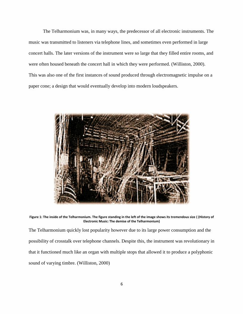
The Telharmonium was, in many ways, the predecessor of all electronic instruments. The

music was transmitted to listeners via telephone lines, and sometimes even performed in large

concert halls. The later versions of the instrument were so large that they filled entire rooms, and

were often housed beneath the concert hall in which they were performed. (Williston, 2000).

This was also one of the first instances of sound produced through electromagnetic impulse on a

paper cone; a design that would eventually develop into modern loudspeakers.

Figure 1: The inside of the Telharmonium. The figure standing in the left of the image shows its tremendous size ( (History of Electronic Music: The demise of the Telharmonium)

The Telharmonium quickly lost popularity however due to its large power consumption and the

possibility of crosstalk over telephone channels. Despite this, the instrument was revolutionary in

that it functioned much like an organ with multiple stops that allowed it to produce a polyphonic

sound of varying timbre. (Williston, 2000)

7

Then in the 1920‟s a number of instruments were developed that redefined the way

electronic music was produced. The first was the Theremin, invented by Leon Theremin in 1921.

The Theremin was revolutionary in that its dual antenna design removed the need for the

performer to actually touch the instrument. Instead the performer could change the pitch and

volume by varying the position of their hands relative to the two antennae.

Figure 2: Leon Theremin posing with the Theremin, the left loop controls volume while the right loop controls pitch.

The Theremin gained popularity for its uniquely eerie constant tone sound, and was

implemented in many Science Fictions movies at the time. Beginning in the 1940‟s it was also

integrated into popular music. The Theremin‟s hands-off interface made it a difficult instrument

to master. However, the unique sound and playing style had a prime impact on the style and

development of electronic music. (Termen, 2007)

Other instruments that produced a Theremin like sound that arose within the same time

period were the “Croix Sonore”, or Sonorous Cross, and the Ondes-Martenot. The Croix Sonore

8

was developed in 1929 by Michel Billaudot and relied on the capacitance between the antennae

and the performer‟s body, much like the Theremin (Cross Sound, 2010).The Ondes-Martenot

produced a very similar sound but did not incorporate the hands off style of playing. It was also

later expanded to include more timbrel sounds. (Bloch, 2004) While production of the instrument

stopped for a time, a new project called the Ondea arose in 1997 that was based on the Ondes-

Martenot. Then in 2008 another instrument officially called the Martenot was developed by Jean-

Loup Dierstein.

These instruments were the forerunners of electronic instruments, and while they were

very popular among composers of classical, pop, and film music during their time, they also had

a large role in the general development of the electronic music aesthetic.

2.1.2 The Development of Electronic Music as a Style

The rise of electronic music cannot be solely attributed to the actions of individuals, for it

takes many to accept an idea and develop it into a global style. However for any great change to

occur there have to be instigators, and one such instigator of electronic music was Feruccio

Busoni. In 1907 Busoni published Sketch of a New Esthetic of Music, which detailed his thoughts

on the newly developing electronic sources of music and their future in the music world. In his

work he states his opinion of structured musical styles, saying “We apply laws made for maturity

to a child that knows nothing of responsibility…. They [mankind] disavow the mission of this

child; they hang weights upon it. This buoyant creature must walk decently, like anybody else.”

(Busoni, 1962) Busoni goes on to talk about the idea of absolute music and how it cannot be

achieved through rigorous application of forms and structures. He is also quoted as proclaiming

9

the necessity of electronic instruments in the development of music. His most famous statement

and one which stuck with his student Edgard Varese throughout his life was simply, “Music is

born free; and to win freedom is its destiny.” (Busoni, 1962) (Snyder, Ferruccio Busoni)

Another notable figure who preceded, and heavily influenced, Varese was Luigi Russolo.

Russolo was a futurist composer whose manifesto, The Art of Noises (Russolo, 1913), had a

profound impact on the development of musical aesthetics. In his manifesto, Russolo describes

the evolution of sound, and how it must break away from the limitations placed upon it by early

civilizations. In his manifesto, Russolo states that when the exceptional noises of hurricanes,

earthquakes, and the like, are removed, nature is predominantly silent. The discovery of sound

was seen by ancient peoples as a great spiritual development, attributed to godly powers, and

remained a mystery to most. Thus sound was made distinct from the noise of life. Early

civilizations took this and broke it into discreet intervals that were to be used. Thus, music

became structured, and therefore limited. Russolo then describes the development of harmony

and the chord or “complete sound”. What started as pure sounds grew more complex, starting

with the triads and becoming more dissonant. This music became more and more polyphonic to

compete with the “multiplication of machinery” that dulled the emotional impact of pure sounds.

This is where Russolo brings up the advancement of technology. Russolo claims that

orchestras can be broken down into four types of instruments, bowed strings, brass wind

instruments, wood wind instruments, and percussion. However, through technology musicians

can extend beyond these instruments and manipulate sounds and noise. In Russolo‟s eyes

traditional music had becomes so mundane that nothing new could come from it, and that

audiences were always left “waiting all the while for the extraordinary sensation that never

comes.” (Russolo, 1913)

10

Russolo then goes on to explain the aspects of noise, its harmonic and rhythmic nature,

and the six families it can be sorted into. The six families that Russolo describes are:

1. Roars, Thunder, Explosions, Rumbles, Booms, Crashes, Splashes

2. Whistles, Hisses, Snorts

3. Whispers, Murmurs, Mumbles, Grumbles, Gurgles

4. Screeches, Creaks, Rustles, Buzzes, Crackles, Scrapes

5. Percussion noises from hitting wood, metal, skin, stone, etc.

6. Voices of animals and men (usually not speaking or singing)

Russolo concludes by stating that it is up to futurist musicians to bring these noises into

the world of music. They must closely observe the world to determine the specific aspects of

noises that allow them to be used compositionally and harmonically, without compromising their

complex nature. And perhaps most importantly, they must find ways to distinguish and recreate

these sounds so that all sounds can be composed into a master orchestra of noises.

Perhaps the most notable pioneer of electronic music and one who is sometimes referred

to as the father of electronic music was Edgard Varese. Varese was an engineer who was later

trained as a classical composer, and was influenced heavily by Debussy. In 1918 Varese broke

from European styles and moved onto more abstract pieces. His work Hyperprism, featured a

number of percussion instruments and a “Lion‟s Roar” (an improvised instrument made with a

rope pulled through a tube), which caused a riot during its first performance, and ended with half

the crowd leaving in an uproar. Yet Varese‟s piece was later performed by the renowned

composer Leopold Stokowski and numerous lesser conductors. Varese‟s other popular work,

Ionisation, was the first use of a siren, accompanied by 37 percussion instruments, as a musical

device. It was not long before Varese became frustrated with the traditions of orchestrated music

and published his manifesto The Liberation of Sound (Snyder, Edgard Varese: The Father of

Elecronic Music) In this manifesto Varese lamented the absence of the technology capable of

creating the types of sounds he desired. In his manifesto Varese sought an instrument that could

11

produce any range and denomination of pitch and timing. Varese states that many accused him of

attempting to destroy traditional music, yet he claims, “Our new liberating medium - the

electronic - is not meant to replace the old musical instruments which composers, including

myself, will continue to use. Electronics is an additive, not a destructive factor in the art and

science of music. It is because new instruments have been constantly added to the old ones that

Western music has such a rich and varied patrimony.” (Varese, 1936) Despite this, Varese‟s

ideas earned him the distrust of the majority of the musical world. After WWII the technology he

so desperately wanted finally arrived and he began experimenting with new sounds. His “Poem

Electronique” which debuted at the Brussels World Fair in 1958 marked one of his largest

successful performances and opened the eyes of the world to this new style of music.

Another great leap in the technology and style of electronic music began in 1946 when

Pierre Schaeffer began his “research into noises”, at the Club d‟Essai de la Radiodiffusion-

Television Francaise. Schaeffer was not a trained musician, but had been working as a radio

engineer when he began a revolutionary technique in sound manipulation that would soon come

to be known as “musique concréte”, or concréte (real) music. Schaeffer began by recording

fragments of sounds with phonographs, whether they be musical or not, and combining them into

collages. In 1948, Schaeffer broadcast his first public pieces of musique concréte, labeled “noise

etudes”. They were entitled “Etude aux Chemins de Fer” or “Study of Railroads”, “Etude Aux

tourniquets”, “Etude aux casseroles”, “Etudes pour piano” (actually two pieces) and “Etude pour

orchestra”. These Etudes helped introduce the use of sampled sounds as compositional material,

particularly “Study of Railroads” which implemented the sounds of locomotives. In “Study of

Railroads”, Shaeffer isolated rhythmic leitmotivs and, through mixing, created both musical and

dramatic sequences. These dramatic sequences were considered to be unmusical until Schaeffer

12

used spectral transposition to alter specific envelopes of sound and create musical sequences.

However, like many of the other unconventional pieces at the time, this was met with a great

degree of opposition.

In 1950 Schaeffer collaborated with Pierre Henry to produce “Symphonie pour un home

seul” which was a 12 movement piece featuring the sounds of the human body. A year later

Schaeffer began experimenting with magnetic tape recorders, which revolutionized the way

musique concréte was produced. The magnetic tape recorder removed the need for multiple

phonographs to provide various samples, and allowed sounds to be cut, spliced, and transformed

with ease; or at least with ease relative to the time. (Ankeny)

Musique concréte was more than just a fancy method of organizing sampled sounds. It

was a completely new approach to music. In Machine Songs V, Carlos Palombini describes

musique concréte as an inversion of the traditional approach to composing. Instead of mentally

conceiving a piece, copying it down in notation, and then having it performed, musique concréte

cannot be conceived prior to its performance, it is conceived by experimentation and compiled

into its final form by the composer. It was due to its experimental nature that musique concréte

tended to sound less like a new form of music and more like just an experiment. In Schaeffer‟s

mind it “lacked a theoretical grounding”, and required some sort of method and criteria to

classify the infinite sounds available to sample. The answer to this came in part in 1951 with

Schaeffer and Henry‟s piece Orphee. From this, Schaeffer created the notion of a pseudo

instrument, or sounds and families of sounds that could fill the roles of orchestral instruments.

Despite this, musique concréte was eventually assimilated into the German elektonische Muisk,

(electronic music) genre. For years Schaeffer would struggle with the method of musique

concrete, until finally in 1958 he established the Groupe de Recherches Musicales which moved

13

on from the topic of musique concréte into a more general form of musical experimentation.

Nevertheless, Schaeffer‟s work was paramount in the development of electronic and non-

traditional music, and had a profound influence on composers after his time. (Palombini, 1993)

2.1.3 The Development of Modern Electronic Instruments and Musical Software.

While the advancement of the electronic music aesthetic is credited mainly with the

composers who developed the ideas and styles for it, it is important to note that many of these

composers were limited at first by the technology available to them. Without the advancement of

technology in musical instrumentation and production the ideals of these composers could never

have been realized. In this respect, few developments are as notable as the invention of the music

synthesizer.

The first synthesizer is credited as the invention of Elisha Gray, who created it during his

attempts to develop a working telephone. A battle he eventually lost to Alexander Graham Bell.

Around 1876 he made his first breakthrough with an electric oscillator, a bathtub, and his own

hand. He found this combination could produce a vibration in the bathtub by using his hand as an

amplifier for the electric signal. He then performed a similar experiment using a metal plate and

the body of a violin. Eventually Gray‟s experiments led to the development of the first multi

tonal synthesizer that used a series of eight keys laid out in the manner of a keyboard. While

Gray‟s invention did not become mainstream in its own right, his discovery that music could be

transmitted along steel reeds through telephone wire became an important stepping stone that

other inventors could build from. (Pioneers of Electro-Acoustics)

For years afterward a number of variations of the synthesizer popped up, but it was not

until 1964 that a truly commercial synthesizer was produced. At that time, Bob Moog, a former

14

engineer for the RCA Mark II synthesizer which like many synthesizers at the time filled nearly

an entire room, developed the first synthesizer that was commercially viable in the music

industry. In 1967 the Monkees featured the first Moog synthesizer in their album, Pisces,

Aquarius, Capricorn, and Jones. This marked the first instance of a synthesizer being used in a

popular album. In 1970 Bob Moog developed the Minimoog, the first portable synthesizer, and

his company began to gain popularity until more and more musicians began to use synthesizers

in their work.

In1978 the first digital synthesizer, the Prophet-5, was developed by Sequential Circuits.

Unlike analog synthesizers, these new digital synthesizers were capable of producing polyphonic

sound and were able to store sounds on their microprocessors. One of the more popular and

affordable models of digital synthesizer was the Yamaha DX-7 which was used by a number of

artists including the Beastie Boys, Nine Inch Nails, Depeche Mode, Madonna, and The Cure.

While these types of synthesizers became very popular with many musicians, a good number of

artists continued to use analog models which allowed then to make real time changes to the

sound. (Baker)

Regardless of whether or not they were preferred by musicians, digital synthesizers had a

profound impact on the entire music world especially with the introduction of MIDI. MIDI

stands for Musical Instrument Digital Interface and was revolutionary in that it does not transmit

an actual audio signal. Instead MIDI data contains a number of different messages that

correspond to various musical properties, such as pitch, velocity (or volume), duration, and any

spectral effects such as pitch bend and modulation. In truth, MIDI messages are simply values

ranging from 0 to 127, until they are interpreted in some fashion by a synthesizer or other

interface. In the early days of MIDI devices, there were many issues with transmitting this data

15

from one machine to another due to the lack of an industry standard. This meant that when a

sound was composed on a machine by one manufacturer then transferred onto another there was

a good chance that the sound would be completely different. However, in 1991 the General

MIDI standard solved many of these issues by providing cross manufacturer industry standards

that allowed musicians to compose on one device and then transfer to another with a reasonable

expectation of how it will sound. (Tutorial: History of MIDI)

The creation of MIDI preceded the development of computer software synthesizers,

which first appeared in the 1990‟s, by nearly a decade. Yet in many ways software synthesizers

were a step above analog and digital synthesizers, even with MIDI. This was because they did

not rely on any hardware and could effectively reproduce the sound of any synthesizer. With

various Plug-ins, VST‟s, and emulators a software synthesizer could provide more sounds and

effects than any single synthesizer in the market, and could be easily controlled using a computer

keyboard. (Tutorial: History of MIDI)

While MIDI and software synthesizers were major breakthroughs in the world of music

technology, they are by no means state of the art. Technology has grown rapidly throughout the

past few decades and led to the development of audio programming languages. Audio

programming languages are computer programming languages specifically designed for sound

production or synthesis. Csound, one of the first audio programming languages, was created in

1985 and is primarily a text based language. Csound has been under constant development over

the years and is currently a powerful tool for audio production and synthesis as well as live

sound performance. (Clemens)

Around the same time Csound came out, Miller Puckette, who had collaborated on the

project, came out with a program called Max which, unlike Csound, uses a graphical user

16

interface. This means that instead of using lines of text as code, the user maps a program out

using graphical objects which are connected by patch cords. An example can be seen in Figure 3.

The unique advantage of graphical interface languages like Max is that they are very

good at portraying the program structure in a way that the user can easily understand. In fact,

Max has been described as the lingua franca for interactive music performance software

(Lossius, 2006). Max operates through a series of objects that act as discrete programs linked

together by patch cords that pass messages from the outlets of one object to the inlets of another.

The types of messages that Max supports are based on six basic data types which are: int, float,

list, symbol, bang, and signal. Signal data is used exclusively with the Max Signal Processing

Figure 3: a sample patch in Max, (Matmos)

17

(MSP) extension. Another unique aspect of Max‟s graphic object oriented design is that users

can design their own objects for a specific purpose and transfer then to other programs.

Essentially the user can create layers of programs within an overarching patch. Max patches can

also be bundled into stand alone programs that are often incorporated into other audio production

software. (What is MAX, 2011)

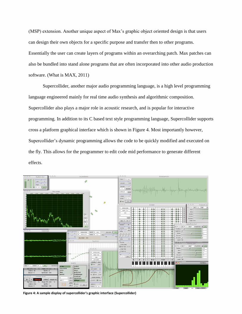
Supercollider, another major audio programming language, is a high level programming

language engineered mainly for real time audio synthesis and algorithmic composition.

Supercollider also plays a major role in acoustic research, and is popular for interactive

programming. In addition to its C based text style programming language, Supercollider supports

cross a platform graphical interface which is shown in Figure 4. Most importantly however,

Supercollider‟s dynamic programming allows the code to be quickly modified and executed on

the fly. This allows for the programmer to edit code mid performance to generate different

effects.

Figure 4: A sample display of supercollider's graphic interface (Supercollider)

18

This idea of real time live programming is perhaps one of the most significant

developments in electronic music. Live programming brings the programmer into the spotlight of

the performance. Where once all computer and electronic music was pre generated in advance,

now the musician can influence the music as it was being displayed. (Supercollider)

All the while other musicians were coming up with more and more unique ways to

perform concerts using innovative instruments and interfaces, such as the laser harp invented by

Bernard Szajner and made famous by Jean Michel Jarre. More recently a new group of musicians

named ArcAttack has arisen with a unique performance that incorporates an enormous Tesla

Coil to produce synthesized musical tones.

So it was that electronic music began in the minds of musicians and composers well

before the technology for such things existed and developed quickly through their ideas and

innovations. Through the exploration of non-traditional sounds and sound generation a number

of unique musical instruments such as the synthesizer and styles such as musique concréte were

born. Then as technology developed even further synthesizers became digital, and then available

in software form and more audio production software arose to the point where the once passive

computer musicians now had an active role in performing their music. Now computer and

electronic music is as common as traditional musical instrumentation and performance.

2.1.4 The Tesla Coil as an Electronic Instrument

In this world of rapidly developing electronic techniques and hardware, the Tesla Coil

has been largely ignored by electronic music enthusiasts, despite the possibilities it presents.

Electronic music is founded on the desire to encompass the full spectrum of sound available in

19

the world, and the Tesla coil presents a great opportunity to experiment with a large variety of

sounds resulting from the unique design of each coil.

Tesla coils in their simplest form can be seen as percussion instruments. The spark

generated by the arc of electricity causes a loud pop or bang that can be repeated with any

desired frequency. If designed correctly, this frequency can be increased beyond the range of

discrete beats, to the point where the rapid sparking of the coil actually produces a tone. A

properly designed and tuned coil can hit any range of notes, well beyond that of human hearing.

This allows for infinite possibilities in notes and scales. However, this itself is nothing new and

was accomplished years ago with the Theremin and other constant tone instruments.

What makes the Tesla Coil unique is that it is one of the very few electronic instruments

that produce the sound themselves, without the use of a loudspeaker. The Tesla coil is itself the

loudspeaker, generating the variation in air pressure through the sudden heating and cooling, and

thus the rapid expansion and contraction, of the air around the spark. More so, a Tesla Coil can

be designed to provide varying levels of distortion, creating an even broader spectrum of

possible sounds. The most common forms of Tesla Coils built for performances are large and

have a sound related to early synthesizers and are often very heavily distorted. The most well

known group to implement musical Tesla Coils is Ark Attack, a group of engineers and

musicians who were the first to develop Tesla coils specifically designed for musical production.

In these cases the pitch of the Tesla Coil is controlled through an outside MIDI controller and

sound synthesizer that feeds the frequency to the coil.

However, the Tesla Coil is also unique in that it can be modulated with any type of

electrical signal, including any type of audio signal. This means it can be substituted as a

20

loudspeaker to play sounds from any source. If designed to have a low resonant frequency the

Tesla Coil will sound more distorted. Alternatively Coils can be tuned at very high resonant

frequencies, which can provide nearly flawless sound reproduction for certain frequencies. This

has led to Tesla coils and variations of the design, to be used as high quality tweeters for sound

systems.

Thus, in addition to providing a unique and interesting means of musical performance

with a distinct sound and visual effect, the Tesla coil could revolutionize the loudspeaker

industry. The sudden rush of interest into electronic music has come hand in hand with an

expansion of music technology, primarily through the continued development of technology like

this. The Tesla coil literally creates sound through the manipulation of electricity in the air, and it

may be that in the future this technique could be expanded further into the electronic music

aesthetic.

2.2 The Development of the Tesla coil and Singing Arc

The Tesla Coil itself has been around for over a century yet it has never truly been a

commercial device. The reason for this is the dangers inherent in working with high voltages,

which explains why the majority of Tesla Coils among the general public are built by

professionals or Tesla Coil enthusiasts. However the possibilities of a Tesla Coil as a unique and

innovative performance device are astounding, and in time there is a good chance that this type

of device will come further into the spotlight.

21

The Tesla Coil was developed in 1891 by Nikola Tesla as a tool to conduct various high

voltage, high current experiments. One of the major uses for Tesla‟s early coils was high

frequency lighting. Tesla conducted numerous experiments with fluorescent and incandescent

lamps as well as high frequency arc lighting. This research led him to develop the first high

efficiency high frequency lighting ballasts. Without this discovery modern Metal Halide Lamps

would not be possible. (Twenty First Century Books, 2011)

One of Tesla‟s earliest discoveries using electrical resonance was that it is possible to

eliminate one of the conductors used to carry current form a power supply to an electrical load.

Through „electrostatic induction‟ or „capacitive coupling‟ a circuit can be completed using a

metal plate connected to one of the high voltage leads of the power supply and another plate to

the load. This led to his development of the carbon button lamp and a single wire electrical

motor. Later he also found it was possible to complete the circuit through the ground by

increasing the distance between the plates. Further work with a single wire incandescent lamp

led to Tesla‟s discovery that vacuum tubes can produce x-rays through the process of

Bremsstrahlung. By studying these X-rays, Tesla was one of the first to find the hazards of X-ray

exposure.

An operating Tesla Coil tends to produce a fair amount of Ozone. Tesla used this to

develop a device designed specifically to cause a reaction between oxygen and nitrogen, leading

to the eventual production of solid nitrogen compounds form atmospheric nitrogen.

Some of the most important experiments Tesla conducted with his coils where those with

wireless telegraphy and telephony. By replacing high frequency alternators with his resonant

transformer, he was able to produce radio waves significantly more powerful than previously

22

possible. Tesla continued to experiment with wireless communications and developed the basis

for many aspects of our modern telecommunications systems, as well as other modern electrical

systems. Even one of the first particle accelerator designs featured a Tesla Coil as its source for

high voltage. (Twenty First Century Books, 2011)

Tesla did not perform many experiments concerning audio applications for the Tesla

Coil. The first exhibited instance of audio modulation of plasma was in 1900 by British physicist

and electrical engineer, William Duddell. Duddell found that by varying the voltage supplied to a

Carbon Arc Lamp (a lamp typically used to provide street lighting before the invention of the

electric light bulb), he could change the pitch of the humming produced by the arc. Duddell

attached a keyboard to the lamp and was able to produce audible tones, thus creating the first

electronic instrument. Unfortunately this instrument became little more than a novelty and

Duddell did not patent it. (William Du Bois Duddell)

2.3 Modern Applications

Today, Tesla‟s original coil designs, and close adaptations of them, are most often built

by hobbyists and electrical engineers for private projects. However the original designs were

adapted and refined and can be considered the predecessor to modern flyback transformers, and

the ignition system in internal combustion engines. Although these devices do not use resonance,

they store energy through an inductive “kick” much like the Tesla Coil stores energy. Tesla Coil

designs are often used in high voltage labs for experimentation, and low power coils are

occasionally used as high voltage sources for Kirlian photography.

23

While there are many instances of Tesla Coils or Tesla Coil descendants in many areas of

modern technology, the main topic of this section concerns the design and use of Tesla Coils as a

musical device on a professional and amateur level.

2.3.1 Professional use of Musical Tesla Coils and the ‘Plasma Speaker’

The first instance of a musical Tesla Coil was a performance by the group Arc Attack.

Arc Attack formed in 2005 and built the first musical Tesla Coils with the help of Steve Ward,

an electrical engineer from Illinois. Since then, they have become a popular performance group

and one of the most well known examples of musicians using Tesla Coils. The group implements

two large custom engineered and built Tesla Coils that produce sounds similar to those of early

synthesizers. This is augmented by a robotic drum set and live instrumental performances by the

crew. (Arc Attack)

Another famous example of a musical Tesla Coil is the performance by Steve Ward at

Duckon 16, an annual science fiction convention held in the Chicago area. In this performance

Steve Ward also used a pair of large Tesla coils that again produced sounds similar to old

synthesizers. (Ward, 2007) While there are numerous examples of performances using large,

heavily distorted coils, the majority of experimentation and innovation in the area comes from

personal projects by electrical engineers and professionally crafted speaker designs by

corporations.

Plasma Speaker is a term used to refer to a loudspeaker that produces sound via the

expansion and contraction of air caused by the manipulation of a plasma arc or flame. The

24

varying temperature of the arc causes rapid expansions and contractions in the air, producing

sound waves. Many claim that plasma tweeters provide a far better quality sound than

conventional speaker because of the lack of weight in the driver. In tweeter design, one of the

main qualities to incorporate is a lightweight dome, and in plasma speakers the dome is

essentially mass less, leading to less distortion and higher transient response. While this is great

news for tweeter design, plasma arcs are not efficient at moving large quantities of air, making

them less suitable for lower frequencies.

2.4 Conventional Speaker and Sound System Design

In order to fully understand how unique Plasma Speakers are in the way in which they

produce sound, it is necessary to look at how conventional speaker drivers operate. In a

conventional loudspeaker, sound is generated by the oscillations of a paper, plastic, or metal

cone in the surrounding air. These oscillations produce pressure waves in the air that we interpret

as sound. The cone is driven by a coil of wire, called the voice coil, attached to an extension of

the cone, called the “former”. The voice coil is suspended inside a permanent magnet so that it

lies centered between the magnet pole pieces and the front plate of the driver. The ends of the

voice coil are connected to the crossover network which is mounted on the speaker binding posts

on the rear of the enclosure. The voice coil is kept centered in the gap by a “spider” attached to

the frame of the driver, and a dust cap mounted at the center of the cone prevents air from

entering from the front of the speaker. In low and mid range speakers there is a rubber surround

connecting the outer edge of the cone to the frame which allows for more flexible motion of the

cone. Figure 5 displays the typical conventional speaker driver design.

25

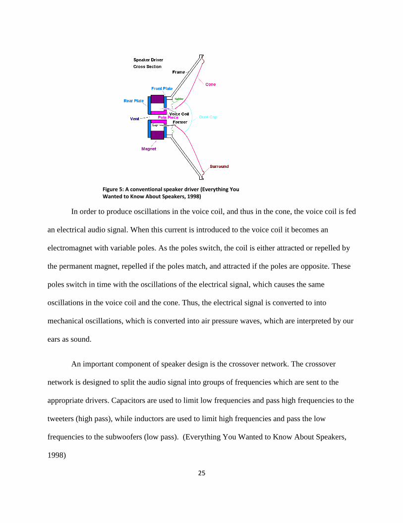
In order to produce oscillations in the voice coil, and thus in the cone, the voice coil is fed

an electrical audio signal. When this current is introduced to the voice coil it becomes an

electromagnet with variable poles. As the poles switch, the coil is either attracted or repelled by

the permanent magnet, repelled if the poles match, and attracted if the poles are opposite. These

poles switch in time with the oscillations of the electrical signal, which causes the same

oscillations in the voice coil and the cone. Thus, the electrical signal is converted to into

mechanical oscillations, which is converted into air pressure waves, which are interpreted by our

ears as sound.

An important component of speaker design is the crossover network. The crossover

network is designed to split the audio signal into groups of frequencies which are sent to the

appropriate drivers. Capacitors are used to limit low frequencies and pass high frequencies to the

tweeters (high pass), while inductors are used to limit high frequencies and pass the low

frequencies to the subwoofers (low pass). (Everything You Wanted to Know About Speakers,

1998)

Figure 5: A conventional speaker driver (Everything You Wanted to Know About Speakers, 1998)

26

In addition to the standard cone style speakers, there is a type of driver that employs a

thin foil or flat membrane. These are called ribbon speakers and use either a thin metallic foil

ribbon or non metallic membrane connected to foil. These membranes are suspended between

permanent magnets, much like the voice coil in cone speakers, and oscillate when a current is

applied. In electrostatic speakers the membrane is coated in powdered graphite which is

connected to a positive charge of several thousand volts. The membrane is flanked by perforated

sheets of metal through which the audio signal is sent, causing them to attract or repel the

membrane as the signal fluctuates. These types of speakers are exceptional at producing mid and

high range frequencies but tend to suffer in the low ranges. Figure 4 shows the basic design of

electrostatic speakers.

Another important aspect to consider when comparing speakers is the impedance of the

speaker. The impedance of the speaker is the amount of resistance the signal from the amplifier

encounters while passing through the speaker. In most designs the impedance is nominally

Figure 6: Electrostatic ribbon speaker design (Audio File)

27

8ohms but in some cases it can be 6 or 4 ohms. Nominally means that the average resistance is

8ohms, however since the resistance can vary with frequency, the range of impedance could be

from 3 to 20 ohms. Impedance has a significant effect on the current drain from amplifiers since,

according to Ohm‟s law: V=IR, (Voltage =Current x Resistance) and the Power Function: P = VI

(Power = Voltage x Current), a speaker with an impedance of 4ohms will draw twice as much

current at a given voltage as a speaker with an impedance of 8 ohms. This means that at any

given power, the voltage drop for a 4 ohm speaker will be divided by a factor of 1.414 while the

current will be multiplied by a factor of 1.414 when compared to an 8 ohm speaker. This means

that the amplifier for a 4 ohm speaker will have to provide a significantly increased current at

higher volumes.

Theses are just some of the factors to consider in speaker design, all of which are very

important. However, the main topic that will be in question here is the effect of the cone material

on sound. There is one major choice that determines what sort of material is used in driver cone,

and that choice is between uniform motion, or rigidity and self damping. Other issues that often

arise are cavity resonance and magnetic non-linearities, all of which are interesting to consider

when using a plasma speaker.

The rigidity of a driver corresponds to the accuracy of the translation of the signal from

the voice coil to the cone. Basically, a higher rigidity means a flatter response, fast pulse rise

time, low IM distortion, and a more transparent sound. These are all important and good

attributes to have, however the more rigid the cone is, the stronger its resonances become. This

can cause certain frequencies to sound stronger and longer. This is partly the result of the poor

coupling between a rigid body and the surrounding air. This poor connection means that the air

28

does not act as a very strong damping force on the cone and the cone will ring for a long time.

This is a problem for loudspeakers which are required to produce a lot of different frequencies

rapidly. The solution to this is to introduce more damping either through amplifier damping or

the intrinsic qualities of the cone.

Ideally the amplifier would, by acting through the voice coil, stop the cone completely

rather than leaving it to ring. In reality the coil only dampens a portion of the cone and other

methods of damping are required. Often rubber surrounds are placed partway down the cone to

add some damping. In this case a lot of attention has to be paid to the damping effect of the

spider and surround materials. Even with the best Kevlar, carbon-fiber, and aluminum cones,

there is always one high Q peak somewhere within the 3 to 5 kHz range. This is unfortunately

right around where the ear is the most sensitive which makes it difficult to deal with, even with a

sharp crossover or notch filter. An alternative is to use a highly lossy (soft) material, usually

polypropylene in most modern speakers. In this case the cone damps itself, however lossy

materials tend to have strange hysteresis modes which lead to IM distortion.

Another issue that typically arises is cavity resonance. Cavity resonance is the result of

high-Q peaks forming in the small spaces between the dust cap and pole piece of the magnet. In

most cases these peaks are high frequency and directional. This often misattributes them to a

problem with the tweeters rather than the mid range speakers, which is where they typically

occur. The other major issue of magnetic non-linearity results from a varying of the inductance

of the iron core pole piece of the magnet. As the coil moves, the inductance of the iron core

varies which causes the roll off frequency to constantly shift. This can also result in significant

IM and FM sidebands throughout the entire frequency spectrum when very deep bass is played,

29

which results in a blurriness to the sound.

It can be seen that there are a number of problems inherent in modern speakers that

inevitably lead to compromises depending on what sort of sound is pursued. This holds true for

plasma speakers as well. However there are some attributes of plasma speakers that make them

unique and in many ways better than conventional speakers.

Plasma speakers are unique in that they have absolutely no resonance, and the best

speakers have an accurate pulse and frequency response up to 100 kHz. This is because they are

effectively mass less, meaning that they have an infinitesimally small transient response. The

driver actually has a mass equal to that of the surrounding air, which means the acoustic coupling

is 1:1. The drawbacks of conventional plasma speakers is that they are often inefficient as they

require a very high voltage to operate, and either produce ozone (for speakers that use ionized

air) or require a constant, somewhat expensive fuel (in the case of helium based speakers). An

alternative to this is flame speakers which would use a combustible material to create a flame

that could then be modulated like any plasma. However, this type of design has not been

explored to any great degree. (Olson, 2001)

2.5 Tesla Coil Designs

The following section describes the three main Tesla Coil designs and their functionality

as musical tools. The first design to be examined is the conventional or Spark Gap driver. This is

the simplest design, but is less suitable for audio modulation than the others. Next we will cover

the Solid State Tesla Coil (SSTC), which is the most common design used for audio modulation.

30

The main difference between the two designs is the replacement of the spark gap with solid state

switches. Thirdly, this section will look at the Dual Resonant Solid State Tesla Coil (DRSSTC)

design and highlight its advantages and disadvantages over the SSTC. The fourth section will

describe the secondary coil and the process of finding its resonant frequency. Finally we will

examine the process of pulse width modulation (PWM).

2.5.1 Spark Gap Tesla Coil

A classical spark gap Tesla Coil includes two main stages of voltage increase. The first

being a conventional iron core transformer, and the second being the air core transformer formed

by the resonant coils. The driver circuit for a spark gap Tesla Coil consists of the iron core

transformer, a capacitor bank, a spark gap, and the resonant air core transformer. Figure 7

displays a schematic for a spark gap Tesla Coil.

This circuit consists of the driver, which includes the iron core transformer, the spark gap

G, capacitor bank C1, and primary coil L1. The schematic also shows the secondary coil circuit

Figure 7: The Classical Tesla Coil (Johnson, 2009)

31

which consists of the secondary coil L2 a ground, and the combined capacitance of the windings

of L2 and the top load of the coil. The capacitor bank of the driver is typically a low loss, high

voltage capacitor that is used to build up charge before the spark gap activates. The spark gap

itself acts as a switch that closes when enough voltage has been built up. Typically, the spark gap

simply consists of two metal spheres separated by a small air gap. When the gap is not sparking

the primary coil acts as a short and the capacitor is being charged by the iron core transformer.

This is shown in Figure 8.

While the Spark gap is not conducting, the iron core transformer is increasing the AC

voltage input, causing the capacitor bank to build up charge. The primary coil acts as an

inductor, opposing the change of current and building up energy in the form of a magnetic field.

When the spark gap activates it allows the circuit to oscillate, effectively becoming an RCL

Oscillator with the spark gap as the main source of resistance. The circuit will oscillate at a

frequency determined by C1, L1, L2, and C2.

When the gap is active, the complete circuit diagram for the driver circuit and secondary

coil can be shown by Figure 9.

Figure 8: C1 Being Charged With Spark Gap Open (Johnson, 2009)

32

Figure 9: Lumped circuit model of a Tesla coil with active arc. (Johnson, 2009)

During this time, the energy stored in C1 is dispersed throughout C1, C2, L1, L2, and M

where M is the mutual inductance of the Primary and Secondary circuits and R1, and R2 are their

respective resistances. If designed correctly, all of the energy in the Capacitor bank can be

transferred to the secondary coil within a certain time t. This means that at time t there is no

voltage across C1 and no current across L1. If the gap is opened at this point then there is no way

for the energy to be transferred back to C1. This causes the Secondary to act as a separate RCL

circuit that oscillates with a frequency determined by C2 and L2. If a proper tuning of the two

circuits is found, it is possible to build very large voltages in the Secondary, leading to large

discharges. (Johnson, 2009)11

2.5.2 Solid State Tesla Coil

A Solid State Tesla Coil operates differently from a classical spark gap coil in that it

implements bi-polar junction transistors (BJTs), metal-oxide semiconductor field effect

33

transistors (MOSFETS), or some other form of solid state device to create oscillations. Figure 10

shows a simple Tesla Coil driver circuit using two of these switches.

This design creates a switching cycle during which the two switches alternate between

off and on while a sinusoidal wave current is passed through the system. In the first stage the

first switch is on while the second is off, causing current to flow into the load through T1. Then

the first switch is turned off while the second is turned on, causing the current to flow out of the

load through T2. During this cycle the sinusoidal load current passes through zero at two points,

halfway through the cycle when switch one turns off and switch two turns on, and at the end of

the cycle when they switch back. It is very important that the switch occurs at these points in

order to reduce the switching losses and any voltage spikes or unwanted ringing. This also helps

to improve the load sharing between parallel switches, and reduces the amount of avalanche

stress on series switches. The driver can also be built with a variable circuit using a timer circuit

or a pulse width modulation (PWM) controller. These types of controllers will be covered in later

sections.

The advantage of a Solid State Tesla Coil over a classical spark gap Tesla Coil is that it is

easier to modulate the frequency using PWM controllers or timer circuits. Also, the spark gap on

Figure 10: Sample Solid State Tesla Coil Driver Circuit (Burnett, 2001)

34

a classical Tesla coil is very loud, sometimes louder than the discharge from the secondary coil,

and it can produce intense UV light which is harmful to the eyes. (Burnett, 2001)

2.5.3 Dual Resonant Solid State Tesla Coil.

A Dual Resonant Solid State Tesla Coil (DRSSTC) operates much like a conventional

spark gap Tesla Coil in that it has a similar corona discharge and implements a capacitor bank.

However, instead of the spark gap, a DRSSTC implements a half-bridge of MOSFETS or

IGBTs. The combination of the capacitor bank and solid state switches, both of which are

resonators, gives the DRSSTC its name. This combination leads to better control over the length

appearance, and sound of the spark than a classical Tesla Coil, which means that like a SSTC a

DRSSTC can be audio modulated. One main difference between SSTCs and DRSSTCs is that

SSTC can operate safely in steady state without much danger, while DRSSTC that are driven for

extended periods at resonant frequency run the risk of blowing the IGBTs or causing overvoltage

of the primary capacitor. Thus, more precautions must be made with a DRSST in order to

achieve longevity. Although audio modulation is possible with a DRSSTC, this project will

focus on the SSTC design as it will be easier to produce with the available resources and time.

2.5.4 Secondary Coil Design

The secondary coil of the Tesla Coil is where the voltage is built up before being release

through corona discharge. In simplest terms it can be modeled as a circuit formed by a capacitor

in series with a resistor and inductor. This is shown in Figure 11.

35

The resistance is created by the large amount of wire used, typically hundreds or

thousands of turns, while the inductance is that of a single layer of tightly wound coil, as shown

in Equation 1.

Equation 1: Inductance of a Solenoid (MacDonald, 2009)

In this equation, N stands for the number of turns in the coil, which is often large for

secondary coils. A stands for the cross sectional area of the coil, and ℓ stands for the overall

length of the coil. This is not to be confused with the length of the wire. ℓ is effectively the

height of the coil for most coil designs. The final component, µ is the permeability of free space,

a physical constant equal to 4π*10-7

H/m

The capacitance of the coil is more difficult to determine. While the capacitance of this

simplified example can be modeled as the voltage difference between the top and bottom of the

Figure 11: Sample Schematic of Secondary Coil of a Tesla Coil (Johnson, 2009)

36

coil, most coils include a sphere or toroid at the top of the coil which changes the image of the

secondary coil as shown in Figure 12.

In these cases, the capacitance used to find the resonant frequency of the Tesla Coil, must

include the capacitance of the coil as well as the capacitance of the top load with the ground. To

find the capacitance of a spherical top load we begin with Equation 2.

Equation 2: Capacitance of Spherical Capacitor

Equation 2 shows the capacitance between two spheres, with one sphere placed inside the

other. Figure 13 shows the physical model of this. If b, the radius of the outer sphere, is made

Figure 12: Equivalent Circuit Representation of the Secondary Coil with a Capacitive Load (Johnson, 2009)

Figure 13: Spherical Capacitor (Johnson, 2009)

37

larger the capacitance will drop, eventually reaching a minimum as b→∞. At this point the

equation for the Capacitance of the sphere will be Equation 3.

Equation 3: Capacitance of Spherical Capacitor as b→∞

Another type of top load typically used in Tesla coils is the toroid. The formula for

finding capacitance of a toroid is slightly more complex than that of the sphere, as shown by

Equations 4 and 5.

Equation 4: Capacitance of a Toroid for d/D < 0.25

(5)

Equation 5: Capacitance of a Toroid for d/D > 0.25

In these equations D stands for the toroid major diameter, from outside to the outside,

while d is the toroid minor diameter, the thickness of the ring. This is shown by Figure 14.

In both equations the capacitance is measured in pF and the diameters are measured in

cm. To determine which equation is used it is necessary to find the ratio between the two

Figure 14: Toroid Dimensions (Johnson, 2009)

38

diameters. If the minor diameter is greater than 25% of the major diameter then equation 5 is

used. If the minor diameter is less than 25% of the major diameter then equation 4 is used. These

equations are empirical, and because capacitors have a tolerance of around 20% these equations

will be appropriate.

To find the total capacitance of the Tesla coil, we must find the capacitance of the coil

itself. Medhurst developed a number of empirical equations to calculate this.

Equation 6: Capacitance of a cylindrical coil of wire (Lux, 1998)

Equation 6 is the simplest expression for this capacitance, and shows that the capacitance

in the coil is equal to the diameter of the coil, D, times a factor H. H is determined by the ratio of

D to the length of the coil ℓ. For ℓ/D =2 H =0.51, while for ℓ/D=5 , H = 0.81. For ℓ/D from 2 to

5 this relationship is linear. Equation 7gives H for any value of ℓ/D between 2 and 8.

Equation 7: Formula for Medhurst Constant H, for values between 2 and 8 (Johnson, 2009)

In order to find the total capacitance of the Tesla coil, the individual capacitances of the

top load and the coil must be combined. Since they are connected in parallel the capacitances

will simply be added. However, there are a few factors that influence the resulting capacitance.

When the top load and coil are combined, shielding occurs, causing the total capacitance to

decrease, yet when both are brought near the ground, the capacitance increases. Since these

39

factors oppose each other, the capacitance is typically within 20% of the calculated sum.

(Johnson, 2009)

Once the total capacitance and inductance are found it is possible to find the resonant

frequency of the coil using a second order differential equation.

Equation 8: Differential Equation for Voltage across a Capacitor (Blinder)

This equation can be solved to obtain:

Equation 9: The resonant frequency of a single coil.

Where Fr stands for the resonant frequency of the coil, L stands for the inductance, and C stands

for the total capacitance. Finding the exact resonant frequency of the secondary coil is essential

for most spark gap designs. However for Solid State coil designs it is possible to sweep through a

large range of frequencies so less precision is needed.

2.5.5 Pulse Width Modulation

Although Tesla Coils can be constructed in many ways, most Solid State Coils implement

a technique known as Pulse Width Modulation (PWM) to properly control the flow of current

through the coils. In simple terms, Pulse Width Modulation is the control of the “on” and “off”

40

time of a voltage pulse. This pulse is then applied to some sort of MOSFET or BJT gate which

regulates the flow of current in another part of the circuit.

The simplest way to generate a modulated signal is by using a differential comparator,

and in fact this is what most PWM controller components, such as the TL494 used in this design,

use to generate the signal. In this configuration the differential comparator generates either a

high or low signal based on the relationship between the two input signals. In most cases a

triangle or saw tooth wave is fed into the – input while an audio, or other signal is fed into the +

input. When the audio signal is at a higher voltage than the triangle wave, the comparator will

output a high signal. Likewise, when the audio signal is a lower voltage than the triangle wave

the comparator will output a low signal. This relationship is shown in Figure 15.

Figure 15: Example of pulse width modulation using a triangle wave and audio signal (Cloutier)

As we can see in Figure 15, the relative duration of high and low signals is determined by

the voltage of the + input or audio signal. In the case of a 10 volt peak to peak triangle wave, an

audio signal of a constant voltage of 0v will create a pulse that is 50% high (on) and 50% low

(off) as seen in Figure 15(1). In terms of duty cycle, or the percentage of “on” time, this is 50%.

41

If the audio signal has a higher voltage, as shown in Figure 15 (2), its voltage will be higher than

the triangle wave for a longer period of time, and thus the duration of the high signal from the

comparator will be longer. As the audio signal fluctuates rapidly, the duration of the high signal

output will change. This variable duration is what we call pulse duration, or width, modulation.

This output signal is then amplified and sent to the MOSFET or other switching device,

which only allows current to pass when it receives a high signal from the PWM. For Solid State

Tesla Coils and plasma speakers this switching translates to the sparks produced from the

secondary coil. These sparks occur so rapidly that they replicate the fluctuations of a speaker

driver and cause high frequency pressure waves in the air.

Thus through pulse width modulation, an audio signal is transformed into a series of

discrete high and low signals that vary with the fluctuations of the audio voltage. These signals

then determine the flow of current through the primary coil, which in turn controls the flow of

current in the secondary coil. The flow of current in the secondary coil determines the voltage

buildup and the resulting sparks from the coil, which reflect the fluctuations, and in turn the

sound, of the audio signal. (Cloutier)

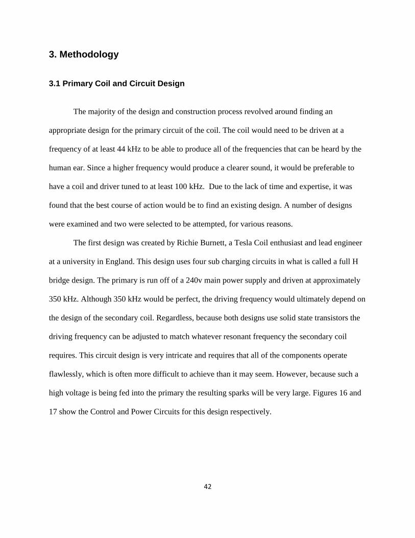
42

3. Methodology

3.1 Primary Coil and Circuit Design

The majority of the design and construction process revolved around finding an

appropriate design for the primary circuit of the coil. The coil would need to be driven at a

frequency of at least 44 kHz to be able to produce all of the frequencies that can be heard by the

human ear. Since a higher frequency would produce a clearer sound, it would be preferable to

have a coil and driver tuned to at least 100 kHz. Due to the lack of time and expertise, it was

found that the best course of action would be to find an existing design. A number of designs

were examined and two were selected to be attempted, for various reasons.

The first design was created by Richie Burnett, a Tesla Coil enthusiast and lead engineer

at a university in England. This design uses four sub charging circuits in what is called a full H

bridge design. The primary is run off of a 240v main power supply and driven at approximately

350 kHz. Although 350 kHz would be perfect, the driving frequency would ultimately depend on

the design of the secondary coil. Regardless, because both designs use solid state transistors the

driving frequency can be adjusted to match whatever resonant frequency the secondary coil

requires. This circuit design is very intricate and requires that all of the components operate

flawlessly, which is often more difficult to achieve than it may seem. However, because such a

high voltage is being fed into the primary the resulting sparks will be very large. Figures 16 and

17 show the Control and Power Circuits for this design respectively.

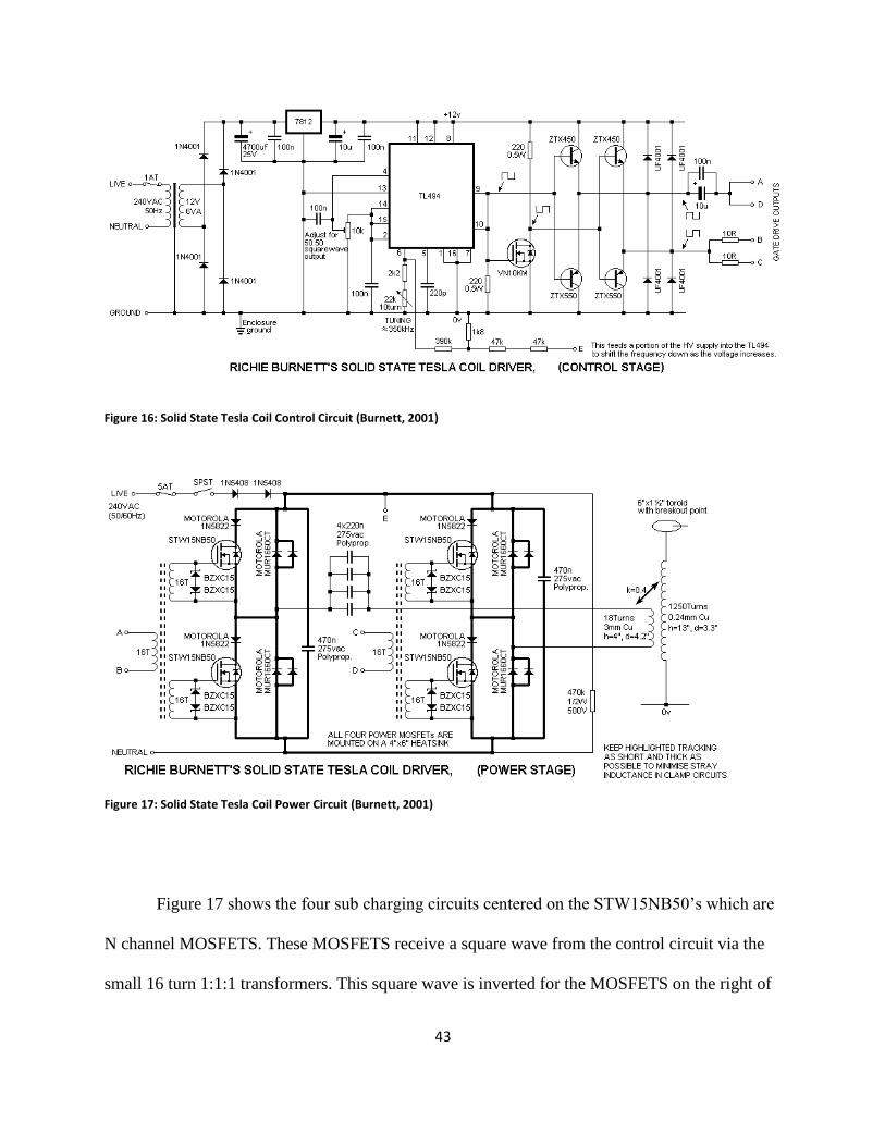
43

Figure 16: Solid State Tesla Coil Control Circuit (Burnett, 2001)

Figure 17: Solid State Tesla Coil Power Circuit (Burnett, 2001)

Figure 17 shows the four sub charging circuits centered on the STW15NB50‟s which are

N channel MOSFETS. These MOSFETS receive a square wave from the control circuit via the

small 16 turn 1:1:1 transformers. This square wave is inverted for the MOSFETS on the right of

44

the schematic. This means that the two pairs of circuits will be switched out of phase, causing the

current to flow only through one pair of MOSFETS at a time. This is essential for the design to

function and, if done successfully, will increase the amount of current flowing through the

primary coil as the current is “swung” back and forth by the circuits. The Control circuit is a

typical PWM design with a few adjustments. The VN10KM component is a special N channel

enhancement mode MOS transistor. Its basic purpose in this design is to change the phase of the

square wave so that the second output is 180 degrees out of phase with the first. The rest of the

additions to the control circuit are designed to step down the 240 v AC to the 12v DC that the

TL494 requires.

As mentioned before this design is very intricate and all of the components must be

working properly. That being said some of the parts used in the design are now obsolete and can

no longer be purchased. Thus, it was necessary to use substitute parts for many of the

components in the design. This led to some interesting effects that resulted in the circuit drawing

too much current. As a result the fuse in the power circuit would consistently blow and on

numerous occasions, a number of the components would short out and break. After numerous

tests it was decided that the best course of action would be to use the alternative circuit which

had been proven to work.

The second circuit design that was chosen was a simpler design that used only 24V DC to

power the primary coil. It had been used in a previous project and was known to provide results

with the components listed in the design. The circuit was originally modified from a plasma

speaker schematic provided by HV Labs.

45

Figure 18: Unmodified Plasma Speaker Schematic (Hunt, 2008)

Unlike the original circuit, the modified version called for a separate DC voltage source

to power the TL494 PWM controller. This removed the need for the 7812 voltage regulator

shown in the schematic above. Additionally, in order to add more protection to the MOSFETS, a

pair of power diodes where added to give the current an alternative path around the MOSFETS

in case there was a problem with the switching times. The modified schematic can be seen in

Figure 19.

Figure 19: Modified Tesla Coil Schematic (MacDonald, 2009)

46

This design is different from the previous one in that in runs off of DC instead of AC. As

can be seen in the schematic above, there are two connections to the coil, just as there were in the

first design. These leads connect to a center tapped primary coil which is fed 24v DC from the

center tap. One half of the coil is wrapped clockwise while the other is wrapped

counterclockwise. This is shown in Figure 20.

The AC needed to induce the appropriate magnetic field on the secondary coil comes

from the switching MOSFETS. The MOSFETS switch out of phase so that one is off while the

other is on. This creates and alternating current in the primary coil by limiting which direction

the current can flow. The actual coil used for this project was two lengths of 16 AWG wire

wrapped around the base of the secondary coil 4 times each in opposite directions. The wires

were twisted together at the top to form the center tap and the other ends were attached to the

MOSFETS. In order to achieve the best coupling between the Primary and Secondary coils, the

coil was mounted on the bottom edge of the secondary coil and insulated from it with Kapton

film and electrical tape.

Since the PWM controller and surrounding components only required 12v, the majority

Figure 20: (a) The Center Tapped Primary Coil. (b) The Filter for the Primary Coil (MacDonald, 2009)

47

of the driver circuit could be mounted on a breadboard. This eliminated the need for complicated

and time consuming soldering on most of the components. Figure 21 shows the breadboard

supporting the PWM circuit.

Figure 21: PWM circuit mounted on a common breadboard

However, due to the high voltages running through the MOSFETS and power diodes,

these components would need to be connected by something that could handle higher voltages.

Since the components handling this voltage were likely to heat up significantly during operation,

both MOSFETS and all four power diodes were mounted on heat sinks and cooled by small 12v

fans powered from the same source as the PWM circuit. The easiest way to mount the

components was to solder the appropriate connections using lengths of wire. Then a thermal

compound was used to establish a thermal connection with the heat sink and the components

48

were taped in place. Figure 22 and 23 show the mounted MOSFETS and power diodes, and the

Primary Coil mounted on the base of the secondary.

Figure 22: MOSFETS and power diodes mounted on two heat sinks.

Figure 23: Primary coil mounted on the base of the secondary.

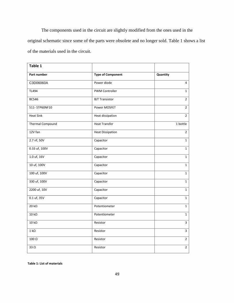
49

The components used in the circuit are slightly modified from the ones used in the

original schematic since some of the parts were obsolete and no longer sold. Table 1 shows a list

of the materials used in the circuit.

Table 1

Part number Type of Component Quantity

C3D06060A Power diode 4

TL494 PWM Controller 1

BC546 BJT Transistor 2

511- STP60NF10 Power MOSFET 2

Heat Sink Heat dissipation 2

Thermal Compound Heat Transfer 1 bottle

12V fan Heat Dissipation 2

2.7 nf, 50V Capacitor 1

0.33 uf, 100V Capacitor 1

1.0 uf, 16V Capacitor 1

10 uf, 100V Capacitor 1

100 uf, 100V Capacitor 1

330 uf, 100V Capacitor 1

2200 uf, 10V Capacitor 1

0.1 uf, 35V Capacitor 1

20 kΩ Potentiometer 1

10 kΩ Potentiometer 1

10 kΩ Resistor 3

1 kΩ Resistor 3

100 Ω Resistor 2

33 Ω Resistor 2

Table 1: List of materials

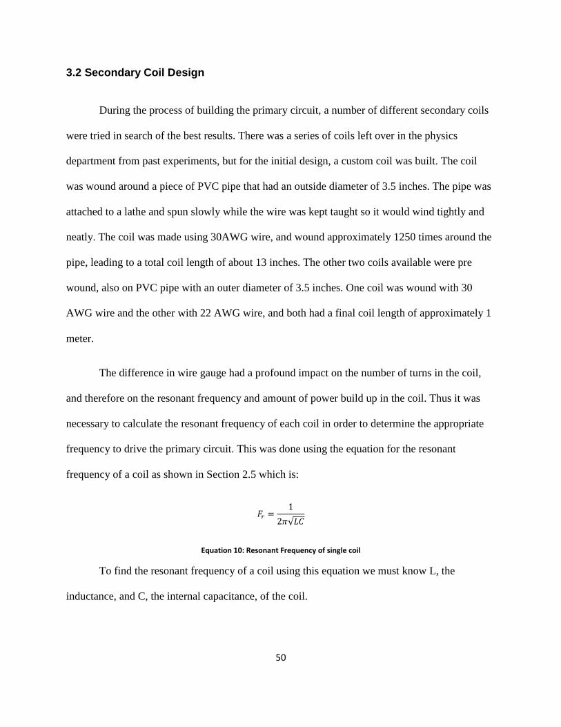
50

3.2 Secondary Coil Design

During the process of building the primary circuit, a number of different secondary coils

were tried in search of the best results. There was a series of coils left over in the physics

department from past experiments, but for the initial design, a custom coil was built. The coil

was wound around a piece of PVC pipe that had an outside diameter of 3.5 inches. The pipe was

attached to a lathe and spun slowly while the wire was kept taught so it would wind tightly and

neatly. The coil was made using 30AWG wire, and wound approximately 1250 times around the

pipe, leading to a total coil length of about 13 inches. The other two coils available were pre

wound, also on PVC pipe with an outer diameter of 3.5 inches. One coil was wound with 30

AWG wire and the other with 22 AWG wire, and both had a final coil length of approximately 1

meter.

The difference in wire gauge had a profound impact on the number of turns in the coil,

and therefore on the resonant frequency and amount of power build up in the coil. Thus it was

necessary to calculate the resonant frequency of each coil in order to determine the appropriate

frequency to drive the primary circuit. This was done using the equation for the resonant

frequency of a coil as shown in Section 2.5 which is:

Equation 10: Resonant Frequency of single coil

To find the resonant frequency of a coil using this equation we must know L, the

inductance, and C, the internal capacitance, of the coil.

51

To find C we can use the Medhurst formula for finding the capacitance of a cylindrical

air core coil. In section 2.5 we had the equation:

Equation 11: Formula for Medhurst Capacitance

Where H is:

Equation 12: Equation for Medhurst Constant for 2< ℓ/D < 8

for values of ℓ/D between 2 and 8. To find out if this equation is appropriate we must simply

calculate the ratio of our coil length over the coil diameter. Which in this case is:

1m/ 0.0889m = 11.24.

Equation 13: Calculation of ℓ/D

Since this value is greater than 8 we must use an alternative formula for H which is:

Equation 14: Formula for Medhurst Constant (Jermanis)

Plugging in the values for ℓ and D we get:

Equation 15: Calculation of Medhurst Constant

52

So for our two coils of length 1m our capacitance will be:

Equation 16: Calculation of Medhurst Capacitance

The next step is to find the inductance of the coil which is given by the equation:

Equation 17: Equation for inductance of a solenoid

Where N is the number of turns, A is the cross sectional area of the solenoid, ℓ is the length of

the coil, and µ is the permeability of free space. The resonant frequency for all the coils was

calculated but for simplicity‟s sake we will only show the calculations for the coil that was used,

which was the 1m 30 AWG coil. For this coil the number of turns, after making adjustment for

the insulation on the wire, came out to be approximately 3921 turns. Plugging this into our

equation for the inductance of the coil we get:

Equation 18: Calculation of inductance of the secondary coil

Now that we have both the inductance and capacitance of the coil we can find the resonant

frequency:

Equation 19: Calculation of resonant frequency of the secondary coil.

Note this resonant frequency may change slightly depending on the type of load placed

on top of the coil. This equation gives the resonant frequency of the coil without any

53

modifications.

To find the resonant frequencies of the other two coils we simply use the same equations

with the appropriate dimensions and number of turns. The resonant frequency calculated for the

long, 1m coil wound with 22 AWG wire is approximately 345 kHz, while the resonant frequency

for the shorter 13inch coil wound with 30 AWG wire was approximately 335.7 kHz. The reason

the taller 30 AWG coil was chosen is because it had the greatest number of turns and would

therefore have the greatest voltage increase when coupled with the primary coil.

During operation the true resonant frequency of the coil was found to be approximately

129.7 kHz which is remarkably close to the calculated frequency. At this frequency the spark

was steady and completely silent when no audio signal was added. Currently the power supply

available is limited to 16v at approximately 3 A. This means that the sound is lower than

expected but it is still audible.

Figure 24: Square wave generated by PWM controller during operation. The frequency is approximately 129.7kHz

54

3.3 Designing the Max program and Musical Interface

The final portion of the project involved creating a non conventional musical interface

that could be added to the coil to create a unique musical instrument. The type of instrument

depended heavily on the materials available. In this case, these were a series of sensors that

output MIDI information that could be processed using various audio programs. The sensors

available were four bend sensors, that output MIDI values from 0 to 127 depending on to what

degree they were bent. The other sensors available were a simple turn sensor that output values

according to its rotation, and a motion sensor that would output a stream of values whenever it

detected a moving object.

The original plan for the interface revolved primarily on creating something that was

biological in nature, and would reflect some aspect human motion, beyond simply playing a note

on a keyboard or other instrument. The bend sensors would be ideal for mapping the motion

joints and so the idea arose of creating a glove with the bend sensors implanted in select fingers.

While there are numerous joints on the human body that may have worked for this purpose, the

hands and fingers provided a centralized location that could include all of the sensors and still

provide fine control for each. Originally the turn sensor and the motion sensor were not going to

be part of the interface. However, during the programming process it was discovered that the

turn sensor could prove to be a useful tool for changing settings in the program without

sacrificing the use of one of the bend sensors. The motion sensor was not included because it did

not allow as much control over the output values as the other sensors.

In order to determine how best to place the sensors so they could interact easily with the

program and each other, it was necessary to determine what purpose each would serve. For that,

55

the program needed to be created. The best option for this was to create a patch in the Max/MSP

program which could easily interface with the MIDI messages from the sensors and transform

them into signal messages. These would then be output from the computer as an audio signal

into the PWM circuit. The patch can be seen in Figures 25 and 26, note that Figure 26 shows the

sub patch that is programmed into the main patch shown in Figure 25.

Figure 25: Max Patch for Music Interface: the leftmost section is the beat generator, the second section is the tone generator, the third section is the recording channel selector and additional effects, and the last section is the loop controls.

Figure 26: Playback object for switching on/off recorded loops.

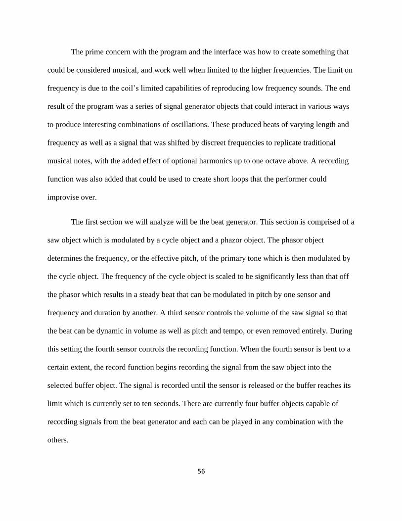
56

The prime concern with the program and the interface was how to create something that

could be considered musical, and work well when limited to the higher frequencies. The limit on

frequency is due to the coil‟s limited capabilities of reproducing low frequency sounds. The end

result of the program was a series of signal generator objects that could interact in various ways

to produce interesting combinations of oscillations. These produced beats of varying length and

frequency as well as a signal that was shifted by discreet frequencies to replicate traditional

musical notes, with the added effect of optional harmonics up to one octave above. A recording

function was also added that could be used to create short loops that the performer could

improvise over.

The first section we will analyze will be the beat generator. This section is comprised of a

saw object which is modulated by a cycle object and a phazor object. The phasor object

determines the frequency, or the effective pitch, of the primary tone which is then modulated by

the cycle object. The frequency of the cycle object is scaled to be significantly less than that off

the phasor which results in a steady beat that can be modulated in pitch by one sensor and

frequency and duration by another. A third sensor controls the volume of the saw signal so that

the beat can be dynamic in volume as well as pitch and tempo, or even removed entirely. During

this setting the fourth sensor controls the recording function. When the fourth sensor is bent to a

certain extent, the record function begins recording the signal from the saw object into the

selected buffer object. The signal is recorded until the sensor is released or the buffer reaches its

limit which is currently set to ten seconds. There are currently four buffer objects capable of

recording signals from the beat generator and each can be played in any combination with the

others.

57

The next section is the tone generator which takes the MIDI data from the sensor and

converts it into a pure tone using the cycle object. Unlike the beat sensor, which produces

continuous tones, a formula is applied to the data going to this cycle object that converts the

values into discrete musical notes. This is done using the equation:

F =

Equation 20: Conversion of MIDI notes into note frequency. (Signal Parameters in MSP, 2010)

Where N is the MIDI value corresponding to pitch, assuming that the MIDI value 69

corresponds to the A above middle C which has a frequency of 440 Hz. This tone can be

accentuated by a secondary tone that can range anywhere from the tonic of the base tone to the

octave above. This allows for a simple method of creating two tone harmonies or dissonant pairs.

This can create interesting effects if the secondary tone is placed at the second or third of the

base tone and the base tone is then shifted rapidly in pitch. Once again the third sensor in this

section controls the volume of these tones and, like the beat generator, they can be removed

entirely if desired. An additional effect in this section is the ability to modulate the volume of the

secondary tone separately. This allows the performer to select a base tone, and then remove it so

that the secondary tone can be modulated freely within a set octave range. This effectively

creates a fine tuned control over pitch within a limited range.

The third section controls the additional effects of the first two sections and allows the

performer to select which buffer object he would like to record with. In this section, the first

sensor controls the volume of an additional effect in the beat generator. The added effect is an

oscillating pure tone that changes in pitch and tempo with the beat produced by the beat

generator. One interesting effect of this tone is a strong bass beat that occurs when its volume is

58

increased. This will not be very discernable with the plasma arc, however if a bass crossover, and

subwoofer, is added to the device it can be used to accentuate the rest of the performance.

In this section, the second sensor controls volume of the secondary tone of the second

section. If the volume of the base and secondary tones is still up when this secondary volume is

increased it will boost the volume of the secondary tone, and often cause it to clip, which creates

some interesting effects. If the volume for the second section is turned down then the secondary

tone will be isolated and the performer will have the fine tuned pitch control mentioned earlier.

The fourth sensor in this section determines which of the four buffer objects the signal

from the beat generator will be recorded to when the recording begins. The sensor is scaled so

that when it is unbent the first buffer object is selected, and the fourth buffer object is selected

when it is fully bent. The recording can only be started while the beat generator section (section

1) is being modified; it cannot be done from any other section.

The fourth and final section is the loop control. In this section, the first sensor determines

whether or not a loop starts or stops. If the first sensor is bent to a certain extend the selected

loop will begin and continue looping until the sensor is released. If the sensor is bent to nearly its

maximum value the loop will play at twice the normal speed. The second sensor determines the

volume at which the loop will play, which can be determined for each individual loop. This

allows for the performer to set up multiple loops to create rhythmic effects. In the Max/MSP

program if the output volume of any signal exceeds a value of 1 the signal will clip. To counter

this, the volume of the loops and most other effects in the patch are limited to 0.2, meaning that 5

different signals can be sent to each of the two channels without the risk of clipping. The fourth

sensor in this section determines which buffer object is being accessed. Just like in the third

59

section this sensor is scaled so that it selects the first buffer object when unbent and the fourth

buffer object when completely bent.

The purpose of the turn sensor is to determine which section is being accessed. There are

five choices that are available to the performer; sections 1-4 and closed. If the closed section is

selected then the data from the bend sensors will not be transmitted to any of the other sections

and the output will remain how it was.

After, and in part at the same time, each sensors function in the patch was decided; a

design for how the sensors would be integrated with the glove was formed. The first three

sensors were placed in the thumb, pointer finger, and middle finger of the right hand, while the

fourth sensor was placed in the thumb of the left hand. The turn sensor was placed in the back of

the right hand glove where it could be easily manipulated by the left hand. This setup allows a

great deal of control of the first three sensors, which are the primary controls for the sound

generation. By placing the fourth sensor in the left hand the sound and recording controls were

separated. This made it easier for the performer to focus on controlling the music with one hand

and recording with the other. Additionally by placing the fourth sensor in the thumb, the

performer could easily manipulate the turn sensor on the right hand without accidentally altering

the recording settings.

60

4. Analysis and Future Improvements.

4.1 Analysis

Figure 25 shows the corona discharge from the coil during operation. When the spark gap

was set to about an inch in length, the spark produced was stable and nearly silent while no audio

signal was added. Under these conditions, the circuit was powered with 24.0 +/- 0.1V and

consistently drew around 7.2 +/- 0.1 A.

When an audio signal was added there was no noticeable distinction in the motion of the

spark, however the audio could be heard quite clearly, if rather quietly. Two different power

supplies were used in the final testing. The first could provide a maximum of 30V at 3As. This

provided enough power to produce a spark and audible music. However, the current cap limited

the voltage to about 16V. Since the amount of power being provided was limited, the size of the

spark and thus the volume of the audio output were reduced. The second power supply had a

Figure 27: Active spark gap from secondary coil.

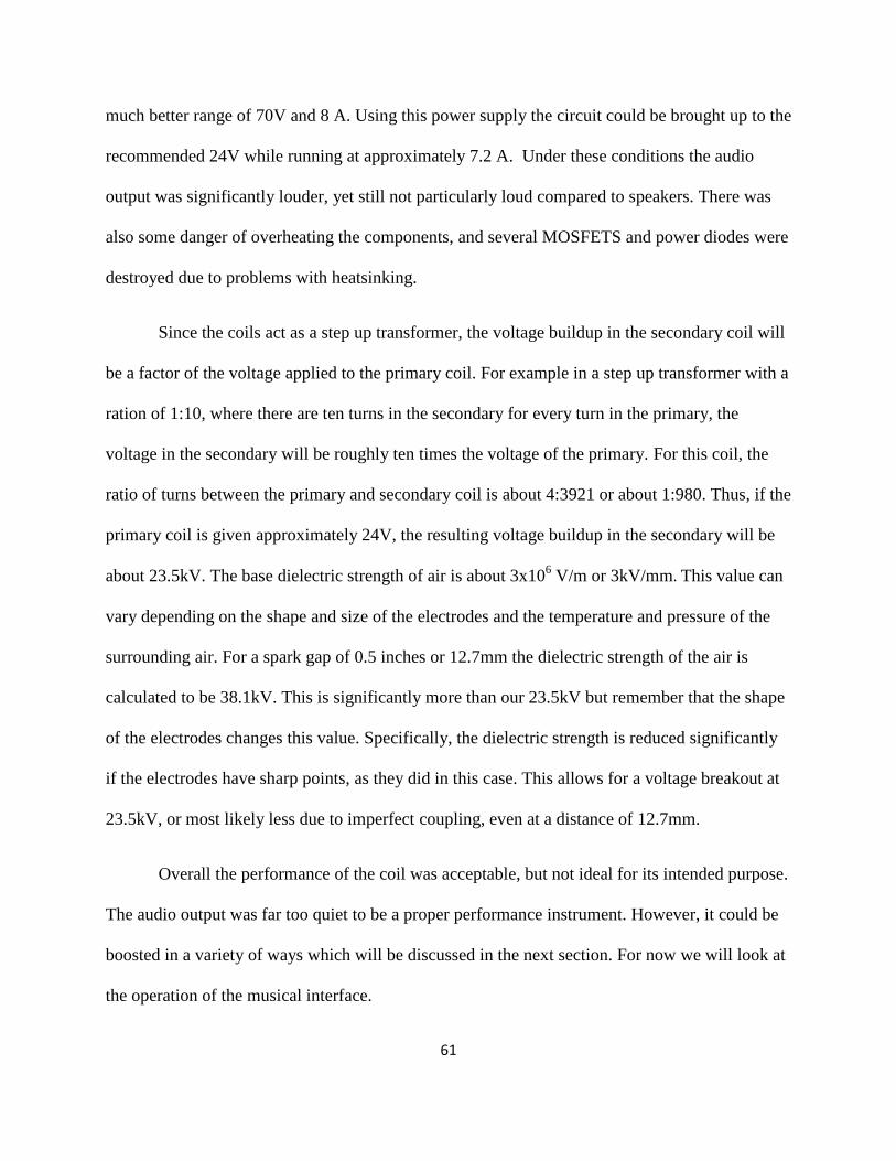
61

much better range of 70V and 8 A. Using this power supply the circuit could be brought up to the

recommended 24V while running at approximately 7.2 A. Under these conditions the audio

output was significantly louder, yet still not particularly loud compared to speakers. There was

also some danger of overheating the components, and several MOSFETS and power diodes were

destroyed due to problems with heatsinking.

Since the coils act as a step up transformer, the voltage buildup in the secondary coil will

be a factor of the voltage applied to the primary coil. For example in a step up transformer with a

ration of 1:10, where there are ten turns in the secondary for every turn in the primary, the

voltage in the secondary will be roughly ten times the voltage of the primary. For this coil, the

ratio of turns between the primary and secondary coil is about 4:3921 or about 1:980. Thus, if the

primary coil is given approximately 24V, the resulting voltage buildup in the secondary will be

about 23.5kV. The base dielectric strength of air is about 3x106 V/m or 3kV/mm. This value can

vary depending on the shape and size of the electrodes and the temperature and pressure of the

surrounding air. For a spark gap of 0.5 inches or 12.7mm the dielectric strength of the air is

calculated to be 38.1kV. This is significantly more than our 23.5kV but remember that the shape

of the electrodes changes this value. Specifically, the dielectric strength is reduced significantly

if the electrodes have sharp points, as they did in this case. This allows for a voltage breakout at

23.5kV, or most likely less due to imperfect coupling, even at a distance of 12.7mm.

Overall the performance of the coil was acceptable, but not ideal for its intended purpose.

The audio output was far too quiet to be a proper performance instrument. However, it could be

boosted in a variety of ways which will be discussed in the next section. For now we will look at

the operation of the musical interface.

62

The musical interface portion of the project was intended to use the bend and turn

sensors, integrated into a glove, to provide MIDI data that the Max/MSP program would use to

generate audio signals. Unfortunately an issue with the sensor interface prevented the output of

the data from the sensors from reaching the program. As it was soon apparent that the interface

would have to be replaced, an alternative method was sought until the problem was resolved.

The sensors were replaced by a series of control knobs on a USB MIDI keyboard. These knobs

output the same range of values as the sensors and worked very well in testing the Max program.

Initially the program only had a number of bugs, primarily related to combining the

various messages from the signal generators into the two channels. This was remedied by

lowering the maximum volume of each signal output to just under 0.2. If a composite signal ever

reached an amplitude of 1 or greater it would clip. This meant that with these new settings up to

five signals could be combined each channel without the risk of unwanted noise. However, this

reduced amplitude meant that the audio output from the coil was also reduced, further limiting

the already low volume level.

While the program and the coil both worked as expected, there were a number of things

that could have been improved to produce more impressive results. If the spark length could be

increased, the volume output would be increased as well making the device more viable as a

performance instrument. The audio quality was quite good, but also could have been improved

by increasing the resonant frequency of the secondary coil. The Max program worked as it was

designed, however the use of the MIDI keyboard removed most of the biological interaction that

was desired. The interface could also have benefitted from a greater number of sensors so that

more joints could be used as controls.

63

4.2 Future Developments

Two options are available to increase the length of the sparks and loudness of the audio.

Either the amount of power being applied to the coil could be increased or the number of turns in

the secondary coil could be increased. If the voltage applied to the primary is increased, the

resulting voltage buildup in the secondary will increase by the ratio of turns. This can lead to a

rather significant increase in output voltage with only a small increase in the initial voltage. The

problem with this is, the increase in voltage will require a larger current, and the power applied

to the primary circuit will increase. This can be dangerous if the components are not properly

heatsinked since there is a good chance they will heat up faster. This can also be dangerous if the

components are not rated for the increased power. Also, because the voltage in the primary and

secondary will be greater, there is a greater chance of arcing between the two, which will require

additional insulation to prevent. Most primary circuits are built with a particular voltage in mind

and it can be complicated to rework the circuit to accommodate higher voltages.

Alternatively, or additionally, to increasing the voltage applied to the primary, the

number of turns in the secondary could be increased. This would increase the ratio of secondary

to primary turns and thus increase the amount of voltage gain. The problem with this approach is

the effect it will have on the resonant frequency of the secondary coil. The secondary coil must

be carefully designed to provide a high enough voltage gain to achieve the desired sparks, yet

still have a resonant frequency high enough to produce all of the audible frequencies. It is also

important to be aware of the range of frequencies to which the primary coil can be tuned. If the

resonant frequency of the secondary coil is outside this range it will be impossible to couple the

two coils together.

64

Improving the musical interface beyond its current state could be as simple as integrating

the gloves and sensors that were originally planned to be a part of the design. Beyond that, more

sensors could be added to provide a greater range of effects and more precise control. Likewise,

the types of sensors could also be modified. There are a number of sensors available that

measure more interesting features of the human body such as heart rate and voltages on the skin

that could be used to produce interesting musical effects that would be more difficult for the

performer to control. This begins to get into the area of subconscious musical performance, in

effect, a performance that is modified by the natural reactions of the body to environmental

effects.

5. Conclusion

The goal of this project was extend my knowledge of electrical engineering and acoustics

and shed some light on the technical and artistic nature of Tesla coils, while attempting to create

a unique and interesting musical instrument. The coil that was created was capable of producing

audible music, and the musical interface was limited only by the lack of properly functioning

equipment. While there are a number of improvements that could be made, the project served its

initial purpose in creating a coil capable of acting as an audio source and illuminating the finer

points of creating such a coil. In addition to providing an example of an interesting form of

musical performance that is largely ignored.

65

Works Cited Ankeny, J. (n.d.). Musique Concrete. Retrieved August 6, 2011, from Allmusic:

http://www.allmusic.com/explore/style/d11002

Arc Attack. (n.d.). Retrieved August 6, 2011, from arcattack.com: http://www.arcattack.com/about.php

Audio File. (n.d.). Retrieved August 6, 2011, from The Audio Advisor: http://eli47.tripod.com/Page2.html

Baker, C. (n.d.). The Synth. Retrieved August 6, 2011, from Open Labs: http://www.openlabs.com/the-

synth.html

Blinder, S. (n.d.). Series RLC Circuits. Retrieved August 6, 2011, from Wolfram Demonstrations Project:

http://demonstrations.wolfram.com/SeriesRLCCircuits/

Bloch, T. (2004). The Ondes Martenot. Retrieved August 6, 2011, from Thomas Bloch: musician

performer of rare instruments: http://www.thomasbloch.net/en_ondes-martenot.html

Burnett, R. (2001). Solid State Tesla Coil. Retrieved August 6, 2011, from Richie's Tesla Coil Web page:

http://www.richieburnett.co.uk/sstate.html#recent

Busoni, F. (1962). Sketch of a New Aesthetic of Music. New York: Dover Publications.

Clemens, j. (n.d.). Csounds. Retrieved August 6, 2011, from Csounds.com:

http://www.csounds.com/about

Cloutier, S. (n.d.). Pulse Width (Duration) Modulators- updated for Solid State Devices. Retrieved August

6, 2011, from Class E radio: http://www.classeradio.com/pdm_article_solid_state.html

Cross Sound. (2010, August 12). Retrieved August 6, 2011, from Scientists of Sounds:

http://chercheursdesons.hautetfort.com/archive/2010/12/08/croix-sonore.html

Everything You Wanted to Know About Speakers. (1998). Retrieved August 6, 2011, from DJ Society:

http://www.djsociety.org/Speaker_1.htm

History of Electronic Music: The demise of the Telharmonium. (n.d.). Retrieved August 6, 2011, from

Music Technology Musician: http://musictechmusician.weebly.com/lesson-1.html

Hunt, O. (2008). Plasma Sonic Speaker. Retrieved August 6, 2011, from HV Labs:

http://www.hvlabs.com/plasmasonic.html

Jermanis, B. (n.d.). Coil Capacitance. Retrieved August 6, 2011, from Nikola Tesla and My Thoughts:

http://free-ri.htnet.hr/Branko/07d2.html

Johnson, D. G. (2009, March 11). Tesla Coil Impedance. Retrieved August 6, 2011, from

http://www.eece.ksu.edu/~gjohnson/TeslaCoilImpedance.pdf

66

Lossius, T. P. (2006). JAMOMA: A Modular Standard for Structuring Patches in Max. Retrieved August 6,

2011, from Jamoma.org: http://www.jamoma.org/papers/jamoma-icmc2006.pdf

Lux, J. (1998, january 24). Medhurst's Formulas for celf capacitance of air-core coil. Retrieved August 6,

2011, from http://home.earthlink.net/~jimlux/hv/medhurst.htm

MacDonald, C. L. (2009). Catapults, Corked Bats, and Tesla Coils: Finding the Truth. Worcester:

Worcester Polytechnic Institute.

Matmos. (n.d.). Retrieved August 6, 2011, from Brainwashed.com:

http://www.brainwashed.com/common/htdocs/discog/ole799.php?site=matmos

Olson, L. (2001). The Family of Direct Radiators. Retrieved August 6, 2011, from Nutshell High Fidelity:

http://www.nutshellhifi.com/library/speaker-design2.html

Palombini, C. (1993). Pierre Shaeffer--From Research into Noises to Experimental Music. Machine Songs

V , 14.

Pioneers of Electro-Acoustics. (n.d.). Retrieved August 6, 2011, from The IDEA:

http://retiary.org/idea/idea2/idea/history/history.htm

Russolo, L. (1913). The Art of Noises. Retrieved August 6, 2011, from The Art of Noises:

http://www.unknown.nu/futurism/noises.html

Signal Parameters in MSP. (2010). Retrieved August 6, 2011, from McGill University:

http://www.music.mcgill.ca/~gary/306/week11/mspfeatures.html

Snyder. (n.d.). Edgard Varese: The Father of Elecronic Music. Retrieved August 6, 2011, from Edgard

Varese: The Father of Elecronic Music: http://homepage.smc.edu/tobey_christine/varese/varese.html

Snyder. (n.d.). Ferruccio Busoni. Retrieved August 6, 2011, from Edgard Varese: Father of Electronic

Music: http://homepage.smc.edu/tobey_christine/varese/busoni.html#references

Supercollider. (n.d.). Retrieved August 6, 2011, from Supercollider: http://supercollider.sourceforge.net/

Termen, L. S. (2007). What is a Theremin. Retrieved August 6, 2011, from Oddmusic: The Theremin:

http://www.oddmusic.com/theremin/what_is_a_theremin.html

Tutorial: History of MIDI. (n.d.). Retrieved August 6, 2011, from MIDI Manufacturers Association:

http://www.midi.org/aboutmidi/tut_history.php

Twenty First Century Books. (2011, May 08). Retrieved August 6, 2011, from Twenty First Century books:

http://www.tfcbooks.com/teslafaq/q&a_045.htm

Varese, E. (1936). The Liberation of Sound.

67

Ward, S. (2007, June 19). Musical Tesla Coils. Retrieved August 6, 2011, from Steve's High Voltage:

http://stevehv.4hv.org/MusicalSSTCs.htm

What is MAX. (2011). Retrieved August 6, 2011, from Cycling74.com: http://cycling74.com/whatismax/

William Du Bois Duddell. (n.d.). Retrieved August 6, 2011, from Todayinsci.com:

http://www.todayinsci.com/D/Duddell_William/DuddellWilliamBio.htm

Williston, J. (2000). Thaddeus Cahill's Teleharmonium. Retrieved august 6, 2011, from

Synthmuseum.com: http://www.synthmuseum.com/magazine/0102jw.html