FEDERAL RESERVE BANK OF SAN FRANCISCO

WORKING PAPER SERIES

Working Paper 2010-27 http://www.frbsf.org/publications/economics/papers/2010/wp10-27bk.pdf

The views in this paper are solely the responsibility of the authors and should not be interpreted as reflecting the views of the Federal Reserve Bank of San Francisco or the Board of Governors of the Federal Reserve System.

The 2007-09 Financial Crisis and Bank Opaqueness

Mark J. Flannery Graduate School of Business Administration

University of Florida

Simon H. Kwan Federal Reserve Bank of San Francisco

Mahendrarajah Nimalendran

Graduate School of Business Administration University of Florida

September 2010

  

The 2007‐09 Financial Crisis and Bank Opaqueness 

By 

Mark J. Flannery 

Graduate School of Business Administration University of Florida 

Gainesville, FL 32611‐7168 Email: flannery@ufl.edu 

  

Simon H. Kwan 

Economic Research Department Federal Reserve Bank of San Francisco 

101 Market Street, San Francisco CA 94105 Email: simon.kwan@sf.frb.org 

 

and 

Mahendrarajah Nimalendran  Email: mahen.nimalendran@warrington.ufl.edu 

Graduate School of Business Administration University of Florida 

Gainesville, FL 32611‐7168  

 

September 30, 2010 

 

 

 

We  are  very  grateful  for  the  excellent  research  assistance  by  Kevin  Cook  and  Sara Wang,  and  for 

comments from Burcu Duygan‐Bump and Don Morgan.  Remaining errors are ours.  Views in this paper 

are  the authors only and do not necessarily  represent  the  views of  the  Federal Reserve Bank of  San 

Francisco or the Federal Reserve System.   

  1

The 2007‐09 Financial Crisis and Bank Opaqueness 

 

 

ABSTRACT 

 

Doubts  about  the  accuracy with which  outside  investors  can  assess  a  banking  firm’s  value motivate 

many  government  interventions  in  the  banking  market.    The  recent  financial  crisis  has  reinforced 

concerns about the possibility that banks are unusually opaque.   Yet the empirical evidence, thus far, is 

mixed.   This paper examines  the  trading  characteristics of bank  shares over  the period  from  January 

1990  through  September  2009.   We  find  that  bank  share  trading  exhibits  sharply  different  features 

before vs. during  the crisis.   Until mid‐2007,  large  (NYSE‐traded) banking  firms appear  to be no more 

opaque than a set of control firms, and smaller (NASD‐traded) banks are, at most, slightly more opaque.  

During  the  crisis,  however,  both  large  and  small  banking  firms  exhibit  a  sharp  increase  in  opacity, 

consistent with  the policy  interventions  implemented at  the  time.   Although portfolio  composition  is 

significantly  related  to  market  microstructure  variables,  no  specific  asset  category(s)  stand  out  as 

particularly important in determining bank opacity.   

   

  1

I.  Introduction and motivation 

The epicenter of  the  recent  financial market  turmoil had been  the  financial  services  industry.  

The  end  of  the  credit  and  housing  boom  in  2006  revealed  earlier  excesses  in  financial markets  that 

eventually led to swollen mortgage delinquencies and the eruption of financial market turmoil in August 

of 2007.   During  the credit boom, asset values were  inflated  in an environment of unusually  low  risk 

spreads, increased financial leverage, and a proliferation of complex financial instruments that proved to 

be fragile under stress.  As market forces corrected these excesses, the simultaneous re‐pricing of risks, 

deleveraging,  and  massive  write‐downs  by  financial  institutions  unleashed  powerful  forces  across 

financial markets.    This  process  would  have  been  painful  enough  if  financial  institutions  had  been 

reasonably transparent.    

However, market participants apparently became unsure about the composition and exposures 

of some financial institutions’ portfolios, and the true economic value of some assets in those portfolios.  

This solvency uncertainty  led  investors to  lose confidence  in the banking system.   At the height of the 

financial crisis, even financial institutions themselves were reluctant to lend to each other, as evidenced 

by the severe dislocation in the interbank funding market (Kwan (2009)).  Some researchers argude that 

borrowing  impediments  reflected  uncertainty  about  counterparty  solvency  (e.g. Heider  et  al.  (2010), 

Pritsker (2010)) – that is, bank opacity. 

Policy makers were concerned about credit flows being disrupted by the substantial amount of 

impaired assets clogging banking firms’ balance sheet. One obstacle to removing  impaired assets from 

banking firms’ balance sheets was the substantial disagreement between  insiders and outsiders about 

the economic value of those  impaired assets.   Furthermore, this kind of  information asymmetry could 

lead  outside  investors  to  undervalue  the  banking  firm’s  equity  in  a  pooling  equilibrium, making  it 

expensive for the banking  firm to raise capital and exacerbating the underinvestment problem (Myers 

and  Majluf  (1984)).  In  an  effort  to  maintain  credit  flows  to  the  real  sector,  the  U.S.  government 

implemented unprecedented policies  to  stabilize  the  financial  sector.   First,  the Troubled Asset Relief 

  2

Program  (TARP)  buttressed  specific  banks’  capital  positions.    Later,  the  Public‐Private  Investment 

Program  (PPIP) was  introduced  to help cleanse banking  firms’ balance  sheets.    In  the  spring of 2009, 

federal  regulators  undertook  a  unique  Supervisory  Capital  Assessment  Program,  or  “stress  test”  to 

assess the solvency of a set of the largest financial institutions.  Market investors apparently viewed the 

stress tests as reducing uncertainty.  Following the release of the stress test results in May of 2009, the 

banking  sector  stabilized and  several  large  institutions  successfully  issued new equity.       While  some 

banking  firms  issued  equity  to  satisfy  regulatory  requirements  upon  the  stress  test  findings,  others 

voluntarily raised a cushion of new equity capital.    

Although the possibility that banking firms are “opaque” has played a central role in the current 

financial crisis, existing empirical evidence on the opaqueness of banking firms is mixed.  Morgan (2002) 

argued  that  bond  rating  agencies  (including Moody’s  and  Standard  and  Poor’s)  are more  likely  to 

disagree  in their assessments of harder‐to‐value firms.   He  interpreted a “split” bond rating, when the 

two main rating agencies  rate  the same bond differently, as a sign of opacity.   Morgan not only  finds 

that banking  firms are more  likely  than nonfinancial  firms  to  carry  split  ratings during his 1983‐1993 

sample  period,  but  also  that  a  bank  holding  company’s  asset  composition  significantly  affect  the 

probability of a  split  rating.    Iannotta  (2006) undertakes a  similar analysis  for bonds  issued  in Europe 

from  1993  through  2003,  and  also  concludes  that  bank  bonds  are more  likely  to  carry  split  ratings.  

However, the European evidence differs from Morgan’s U.S. findings in several ways.  Iannotta does not 

find insurance companies to be more opaque.  He also identifies three industries (construction, “energy 

and  utility”,  and  “other”) with more  splits  than  the  banking  industry  (see  his  Table  3),  raising  some 

question about the true implication(s) of split bond ratings.   

Flannery, Kwan and Nimalendran (2004) (henceforth referred to as FKN)   compared banks’ and 

nonbanks’ equity market microstructure properties and analysts’ earnings forecasts.   During the 1990‐

97  period,  they  find  statistically  and  economically  significant  differences  between  banks’  and  non‐

financial firms’ microstructure properties only for the NASD‐traded firms.  Specifically, they find smaller 

  3

NASD  bank  stocks  were  traded  much  less  frequently  than  a  comparable  nonbank,  despite  having 

comparable bid‐ask spreads.     They also  find  that NASD bank stocks exhibit substantially  lower return 

volatilities and  that analysts predict  their earnings more accurately.   They conclude  that  the assets of 

NASD banks were not unusually opaque but simply boring.  In contrast,  the larger bank stocks (traded in 

the NYSE/AMEX) resemble  their control  firms  in  trading activity, return volatility, and bid‐ask spreads.  

On  average,  investors  seem  to  evaluate  large  banking  firms  as  readily  as  they  evaluate  nonfinancial 

firms.1  

It is important to note that FKN examined banking firms during a relatively tranquil time period.    

It  seems  quite  plausible  that  banks might  become more  opaque  during  broad  financial  crises,  and 

indeed much of the governments’ interventions during the recent crisis were predicated on the market’s 

presumed  inability  to distinguish sound  from unsound  institutions.      It  is  therefore  important  that  the 

sample period for this paper (1990:1 to 2009:9) includes several stressed periods (the early 1990s, LTCM 

in  late  1998,  and  the  recent  financial  crisis)  as  well  as  periods  of  tranquility  (even  euphoria!).  

Furthermore,    the Gramm‐Leach‐Bliley Act of 1999 expanded  the  scope of permissible BHC activities. 

During the recent crisis, some of the uncertainty was associated with activities outside banks’ traditional 

lines of business.  Thus, the earlier U.S.  evidence – mixed as it is – may be less relevant to the current 

banking system, at least at the largest, most complex institutions.     

This paper re‐evaluates the question of banking firms’ opaqueness in the current environment.   

We are  interested  in  three main questions:   Are banks  relatively opaque?   Does bank opacity change 

over time and with broad financial conditions?  Can we link opacity to specific features of a bank’s asset 

portfolio?    To  answer  these  questions,  we  compare  equity  market  trading  patterns  of  banks  and 

nonbanking  firms.    A  primary  idea  from  the market microstructure  literature  is  that  a  firm’s  equity 

                                                            1 A recent paper by Morgan et al.  (2010) examines market reactions  to various announcements about  the 2009 stress  test.   They conclude  that banks are neither  totally opaque nor  totally  transparent.   The market correctly identified which firms would be judged to have sufficient capital, but was somewhat surprised by the announced magnitudes of capital required for the (apparently) under‐capitalized institutions.   Their methodology permits no comparison between banking and other firms. 

  4

trading properties reflect  the nature of  information available to market participants.   A higher bid‐ask 

spread,  for  example,  is  associated  with  a  greater  possibility  that  some  traders  have  information 

unknown to other traders.   A market‐maker therefore quotes a higher spread to protect himself from 

losing money when trading with informed counterparties.  The extent to which trades have a permanent 

effect on a  stock’s value  reflects  the  relative  importance of  informed  (vs. uninformed)  traders  in  the 

market (Kyle (1985)).  Holding constant the bid‐ask spread, trading volume should rise with differences 

of  opinion  about  a  firm’s  value,  and  greater  opacity may  either  broaden  or  narrow  differences  of 

opinion.   

In  this  study, we pursue  two  lines of  inquiry. First, we match  traded bank holding companies 

(BHCs) to nonfinancial firms with similar equity values and prices per share, and compare their market 

microstructure properties over the period 1990:1 through 2009:9.  During normal (non‐stressed) times, 

larger banks  (traded on  the NYSE)  seem no more opaque  than  their nonfinancial  control  firms.   The 

evidence  is  slightly mixed  for  (smaller) BHCs  (traded on NASD).    Their  adverse  selection  spreads  are 

relatively higher, but  their price  impacts are  lower  than  their nonfinancial  control  firms.   Given  their 

lower trading volume and share price volatility, we conclude that NASD banks also are no more opaque 

than their control firms during normal periods.   

However,  during  the  2007‐09  financial  crisis,  results  of  comparing microstructure  properties 

between bank and nonbanks are very different.   Both the spreads and price  impacts of BHC stocks are 

significantly higher than nonbanks, consistent with a sharp increase in opacity in banking firms.  It thus 

appears that bank opacity varies over time.         

Second, we  investigate whether the higher BHC opacity during  the  financial crisis  is related to 

bank asset holdings.   We perform regression analysis to assess whether a bank’s portfolio composition 

has any effects on opacity.   While we find asset composition has significantly different effects on bank 

opacity during the financial crisis, the portfolio source of opacity, however, is somewhat difficult to pin 

down.   

  5

The rest of this paper is organized as follow.  Section II discusses information and equity trading 

properties.  Data and descriptive statistics are presented in Section III.  Section IV provides the results of 

the comparisons of market microstructure properties between banking firms and control firms.  Section 

V presents evidence about the effects of bank portfolio composition on measures of bank opaqueness.  

Section VI concludes. 

 

II. Information and equity trading properties 

The motivation for examining market microstructure properties can be found in Demsetz (1968), 

who  demonstrated  that  a  stock’s  bid‐ask  spread  is  systematically  related  to  several  of  its  trading 

properties.  Bagehot (1971) argues that one of these properties should be the potential for differentially 

(privately)  informed  traders.   Benston and Hagerman  (1974)  study a  sample of more  than 300  stocks 

traded over‐the‐counter, and conclude that  interdealer competition, price volatility, share price, order 

flow, and insider trading all significantly affect a stock’s bid‐ask spread. Roll (1984) model that estimates 

the  bid‐ask  spread  using  the  serial  covariance  of  transaction  price  returns    motivated  a  series  of 

empirical methods for decomposing a stock’s bid‐ask spread into logically distinct components (see, for 

example Glosten and Harris (1988), Stoll (1989), George et al. (1991), Huang and Stoll (1994), and Lin et 

al. (1995)).  A stock’s bid‐ask spread covers several distinct costs of operations.  First, the spread must be 

large  enough  to  cover  the  cost  of  processing  customer  orders.    Second,  the market‐maker  holds  an 

inventory of stock  in order to provide traders with  liquid markets.       The cost of holding this  inventory 

includes both  the  time value of  invested  capital and a  risk premium  for bearing nondiversifiable  risk.  

The third spread component reflects a market maker’s information asymmetry, and requires a bit more 

explanation to relate it to the notion of asset opacity. 

  Market makers  effectively write  options  to  traders when  they  post  bid  and  ask  prices.    The 

market maker expects his offer to be “hit” by  informed traders more frequently  if the bid price  is too 

high or the ask price is too low.  The greater the potential supply of private information about a stock, 

  6

the larger will be the adverse selection (AS) cost of trading it.  Brennan and Subramanyam (1995) report 

that  a  stock’s  AS  component  is  negatively  related  to  the  number  of  analysts  following  the  firm, 

suggesting that greater analyst coverage reduces the importance of privately informed traders.  Krinsky 

and Lee (1996) find that the AS component significantly widens for the two days prior to a company’s 

earnings announcement,  consistent with  the hypothesis  that market makers are more  susceptible  to 

informed trading when earnings are known to insiders, but not yet announced.  Differentially informed 

traders, who  threaten  the market maker’s profits,  should be more  important  at  firms  for which  it  is 

more difficult to find reliable public information about asset value.   If investors in general cannot value 

a  firm’s  assets  very  accurately, perhaps  insiders or  specialized  traders  can.    This may be  particularly 

important for banking firms, whose underwriting and  loan monitoring abilities affect value but may be 

difficult  for outsiders to observe.   Kyle  (1985) therefore concludes that a “more opaque” asset should 

trade with a larger bid‐ask spread.   

  Although  the  AS  component  of  a  stock’s  bid‐ask  spread  constitutes  an  ideal  measure  of 

information asymmetry, it cannot be observed and must be estimated (with error) by fitting transactions 

and quote data  to a  specific model.     For  robustness, we also use a  stock’s effective  spread  (defined 

below) as measures of adverse selection.   2 This implicitly assumes that market makers have about the 

same  operating  costs  for  all  stocks,  so  cross‐sectional  variation  in  their  effective  spreads  captures 

variation in the adverse selection cost of trading.   

  Another measure of opacity comes in the form of price impact.  The price impact is designed to 

capture the permanent (as opposed to the transient) component of the price change due to trades. In 

the Kyle  (1985) model  the price  impact  is  the coefficient λ which  is  the ratio of  the  informed  trader’s  

information  to noise  trader  variance.   Hence,  if  there  is  relatively more  information  in  the  informed 

                                                            2     Note  that  the  bid‐ask  spread’s  components  likely  are  interrelated with  other  facets  of  the  stock’s  trading 

patterns.     For example,  if  information asymmetry  leads to a higher spread, trading volume could fall and hence 

the market‐makers’ order processing costs might rise.   

  7

agent’s  trade,  then  the market maker will  adjust  the  price more  aggressively  as  she  extracts more 

information regarding prices from the trade. Note that in the Kyle model there is no bid/ask spreads. It is 

more like the NYSE specialist market. Where orders are submitted and the market maker sets the price 

after seeing the order flow. The price impact measure that we use is not exactly the Kyle lambda (we do 

not have  this  for  the 1990‐92 period). We estimate  the absolute price change divided by  the volume 

traded. This  is similar  to  the Amihud(2002) measure and  is a proxy  for  illiquidity and  is related  to  the 

price  impact coefficient  λ  in Kyle  (1985). We argue  that an opaque asset would be  less  liquid, cēterīs 

paribus,  as  less  informed  traders will  be more  reluctant  to  trade;  hence  in  theory  our  price  impact 

measure would be a good direct measure of opacity. 

  We also examine two additional trade dimensions whose measurement is more straightforward 

than the preceding three (direct) measures of opacity.  First, trading volume could either rise of fall with 

asset  opacity.    In  theory,  a  perfectly  opaque  asset  could  be  very  liquid.    It would  trade with  no AS 

component  to  its  bid‐ask  spread  because  the market maker  need  not  fear  a winner’s  curse.   A  low 

spread would attract greater  trading volume  (say,  for  liquidity purposes),  further reducing  the market 

maker’s break‐even spread.  However, this scenario is easily disturbed: any possibility that some trader 

may  possess  private  information  about  the  asset’s  value  could  seriously  reduce  its  liquidity.   Higher 

spreads  (due  to  AS)  should  then  discourage  uninformed  traders  from  holding  a  stock  (Gorton  and 

Pennacchi (1990)), making  it more difficult for  informed traders to hide their  information.   In the  limit, 

the market  for opaque  shares could break down entirely, as  in Akerlof  (1970).   However,  the market 

need  not  collapse  if  opinionated  investors wish  to  trade  frequently with  one  another  because  they 

disagree about the correct value of the underlying assets (Harris and Raviv (1993)).  So to the extent that 

more opaque  firms  are  subject  to  greater differences of opinion,  trading  volume might be positively 

related to opacity. 

  It  is  an  old Wall  Street  adage  that  "It  takes  volume  to make  prices move."    Karpoff  (1987) 

reviews  the  literature on  the  relation between  volatility  and  trading  volume  in  financial markets. He 

  8

finds  that volume  is positively related  to  the  (absolute) magnitude of  the price change, and,  in equity 

markets, to the price change per se (positive changes are related to higher volume). He also provides a 

summary of other research in this field.  Bessembinder (1996) investigates the relation between volume 

and proxies for information flow and divergences in opinions.  He finds that volume in individual stocks 

are related to firm specific information flows consistent with Kyle (1985) model of strategic trading. This 

suggests  that volume  should be  related  to Kyle’s measure of price  impact which  in  turn  is  related  to 

information asymmetry and opacity. 

The final measure for opacity we consider is the stock return volatility. There are two origins for 

stock volatility:   Fundamental volatility arises from permanent changes  in the price due to unexpected 

changes  in  the  value  of  the  asset.  This  can  again  be  split  into  a  component  that  is  due  to  public 

information  and  another  component  that  arises  from  the  price  discovery  that  is  inferred  from  the 

informed  trading.  Further,  the  informed  traders will  exert  pressure  on  prices  through  their  trading 

activity and this will change prices during high trading volume days.   Hence, the fundamental volatility 

will be correlated with the AS component of the spread.   Transitory volatility is due to trading activities 

by uninformed,  liquidity, or noise traders, and market frictions such as bid/ask bounce. The changes  in 

price due  to  these  types of  traders are subsequently  reversed and hence  the volatility  is  transitory  in 

nature. Transitory volatility  is related to the costs of trading for uninformed traders and  is  likely to be 

very  small  in  very  liquid markets  (in  our  case  for  large  firms).   We  therefore use  return  volatility  as 

another indicator of opacity, which could be a particularly good proxy when there is an episodic volatility 

event such as the financial crisis. 

  To  summarize,  we  measure  information  opacity  using  five  variables  informed  by  market 

microstructure  theories.    They  are:  (1)  the  adverse  selection  component  of  bid‐ask  spread,  (2)  the 

effective spread, (3) the price impact, (4) trading volume, and (5) stock return variability.3   

                                                            3   Equity trading arrangements have changed substantially over the past two decades, in ways that  might affect 

the measured values of microstructure variables.  First, in April 2001 the SEC required that NASD and NYSE prices 

  9

According  to  theory, more opaque  firms may have a higher  reading  in one or more of  these opacity 

measure(s),  ceteris  paribus.    However,  inter‐relationships  among  the  microstructure  variables 

complicate  their  interpretation.    For  example,  trading  volume  is  positively  correlated  with  return 

volatility  (Karpoff  (1987),  Jones  et  al.  (1994)).    Lower  turnover  is  expected  to  raise  a market‐makers 

operating costs by  lengthening the amount of time s/he must hold shares  in  inventory.   Low volatility 

may have the opposite effect, by reducing  the risk of  inventory positions.4     While the effects of both 

turnover  and  volatility  should  be  reflected  in  ESPREAD,  they  should  not  in  theory  enter  into  the 

computation / estimation of the adverse selection component of spread.  

Among the three direct indicators of firm opacity, we have a slight preference for relyiing on the 

price  impact  measure.    It  is  arguably  less  prone  to  endogeneity  issues,  and  less  model‐specific.  

According to Kyle (1985), trades by informed traders will move the stock price towards its (unobserved) 

fundamental value, while uninformed (“noise”) trades are not expected to have lasting impact on prices. 

 

III. Data 

We  identified a sample of publicly traded bank holding companies (BHCs) that file the Federal 

Reserve’s Consolidated Financial Statements for Bank Holding Companies (FR Y‐9C).  We then examined 

ISSM  (for 1990‐92) and TAQ  (post‐1992)  transactions data  for  these BHCs, and eliminated  firms with 

insufficient  trades  to  permit  reliable  estimates  of  the  firm’s market microstructure  properties.  5      In 

particular, we omitted  any BHC‐quarter  for which  the  stock had  fewer  than 100  trades,  the  average 

                                                                                                                                                                                                be  quoted  in  decimal  increments  or  pennies.    Bid‐ask  spreads  fell  substantially,  as  did  quoted  depth 

(Bessembinder, 2003).  As posted depths fell, however, limit orders have become a much more important part of 

the market’s  liquidity.    Second,  trading  volumes  have  exploded,  in  part  due  to  shrinking  spreads  (transaction 

costs), and in part due to the entry of hedge funds, “flash” traders, and other suppliers of liquidity.  We control for 

these  structural  changes using  time dummies  and matched  control  firms when  evaluating bank microstructure 

variables.    

4 The effect of STD depends on the systematic vs. nonsystematic composition of total volatility. 

5 We omit data for the first three months of 1993, when our TAQ dataset had very few bank observations.   

  10

quoted spread exceeded 10% of the share’s price, or the average share price was less than $2.  We also 

omit any firm‐quarter in which the stock had a split or paid a stock dividend greater than 10%, because 

research  suggests  significant microstructure  changes  following  a  split  (Desai  et  al.  (1998)).    The  final 

sample consists of more than 55,000 firm‐quarters for NASD banks and 14,500 firm‐quarters for NYSE 

banks.   

  In order to compare bank stocks’ trading characteristics to those of nonfinancial firms, we match 

each sample BHC with a control firm on the basis of equity market value, share price, and trading venue 

(NASD or NYSE).       Potential control firms are selected from the set of all CRSP firms that survived the 

entire calendar year, except  financial  firms  (SIC code 6000‐6999) or regulated utilities  (SIC code 4800‐

4900).   We first select the firm whose market value  is closest to the BHC’s.   If that firm’s share price  is 

within 25% of the BHC’s share price, we use this as our nonfinancial control firm.  Otherwise, we select 

the next‐closest equity value match from the proper trading venue, determine if its share price is within 

25% of the BHC’s, and so forth.  Each bank stock’s control firm is re‐selected at the start of each calendar 

year.   We treat the firms that are traded on the NYSE separately from those that are traded on NASD, 

because the two markets have different trading arrangements.6 

For each sample firm, we compute five market microstructure variables related to opacity.  Each 

variable  is computed using all  the  trades  from a given day, and  the daily values are averaged  to give 

monthly observations.  We start with three measures of information asymmetry derived from the stock 

price’s dynamics. 

1) AS: the adverse selection component of the bid‐ask spread (as a proportion of share price), computed using all transactions for the day, as in George et al. (1991). 

 2) ESPREADit:  the  effective  spread  for  stock  i  reflects  trades  that  occur  inside  the  quoted 

spread.  Specifically,   

                                                            6 Each NYSE stock has an assigned market‐maker who must maintain orderly, two‐sided trading in the stock.  NASD 

brokers can enter (or withdraw) quotes without exchange‐imposed restrictions   

  11

  ESPREAD ∑ /  

 where  Pτ = trade price,  

I = indicator equal to unity for a bid‐initiated trade or zero for an ask‐initiated trade (based on Lee and Ready (1991)). 

Qτ = the average of the bid and ask prices associated with the τth trade,  

n  is the number of trades within a day.  

3) IMPACT: the permanent effect of a trade on share price Amihud (2002):    

1 |∆ |10  

 

∆ .   

Qt and Qt+5  are the matched mid‐quotes for the trade closest to five seconds prior to and five minutes after the trade.  

   is the size of the trade or number of shares traded.    n  is the number of trades within a day.   The variable is scaled by 106 to avoid reporting a large number of leading zeros in 

its summary statistics.    

IMPACT should reflect the ratio of informed to uninformed traders in the market. Hence, a higher value  for λ  implies greater  information asymmetry or opaqueness  in the associated stock (Kyle (1985)).   

4) Trading activity (TOVER), measured as the number of shares traded, divided by the average number of shares outstanding during the month.   

5) Daily return volatility (%)  

√ 100  

where  STD  =  standard  deviation  of  the  continuously  compounded  returns  based  on  the quote midpoint associated with each trade within a day.  

n = the number of trades within a day.   

These market microstructure variables’ monthly summary statistics are presented in Table 1.    

IV. Microstructure comparison between BHCs and control firms 

  We  start  with  a  set  of  monthly  comparisons  between  BHCs  and  their  matched  (control) 

nonfinancial firms for five microstructure variables, over the full sample period (1990‐1 through 2009‐9).  

  12

Although we match on share price and firm market value at the start of each calendar year, the matched 

variable values can drift apart during  the  subsequent months.   Because  share price and  firm  size can 

affect some important microstructure variables (e.g. Madhavan (2000), page 205), we control for these 

effects and estimate the following regression:  

μ         (1) 

Where 

  denotes the jth (j = AS, ESPREAD, TOVER, VOL, IMPACT) BHC i’s market microstructure value in 

month t less that of its matching nonfinancial firm; 

Δ   = the inverse of the average share price for BHC i in month t less that of its control firm; 

Δ   = the log of BHC i’s average equity market value in month t less that of its control firm.   

The estimated value of  δ0  thus measures  the mean excess BHC microstructure variable value over  its 

control firm, after controlling for differences  in share price and equity market value between the BHC 

and control.  Equation (1) can be estimated as a pooled time series‐cross section or as a series of (Fama‐

MacBeth (1973)) cross‐sectional regressions.  The panel regression results for the entire sample period 

and  for  several noteworthy  sub‐periods  are  reported  in Table 2.   The estimated  intercept  terms  (δ0) 

from monthly cross‐sectional regressions are presented graphically  in Figures 1  ‐ 5,  in which the NYSE 

and NASD sub‐samples are examined separately because the market structures differ.  In addition, some 

previous research has indicated that these two groups of BHCs differ in their opacity (FKN).    

A. Basic Patterns 

Figures  1A  to  5A provide  the monthly  comparisons  for NASD  firms by  charting  the  intercept 

term δ0  in equation (1) separately for each of the five opacity measures.   Figures 1A and 2A show that 

the adverse selection components of   NASD BHCs’ bid‐ask spreads tend to be significantly higher than 

their controls.  These differences are statistically significant primarily during the 2007‐09 financial crisis.  

However, the price  IMPACT measure  in Figure 3A  indicates that  informed trading  is  less  important for 

BHC than for their control firms.  In Figures 4A and 5A, the price TOVER and VOL of NASD BHCs tend to 

  13

be  significantly  lower  than  their  controls before  the 2007‐09  financial  crisis.   We are  thus  inclined  to 

emphasize  the  IMPACT  implication  that  NASD  BHCs  are  relatively  transparent.      The  relatively  high 

ESPREAD could reflect the net effect of lower turnover and lower STD on the operating cost component 

of spreads, while the AS variable  is based on a market‐maker model that may be  less relevant  later  in 

our sample period.   The time variation  in the microstructure variables  in Figures 1A – 5A suggests that 

microstructure  comparisons  may  vary  over  time,  and  across  financial  market  conditions.    The 

comparisons for NYSE BHCs and their controls differ somewhat from that of the NASD sub‐sample.  First, 

there  is no  indication  in Figures 1B and 2B that NYSE‐traded BHC have higher adverse selection costs:  

both  the  AS  and  the  ESPREAD  monthly  differentials  in  Figures  1B  and  2B  are  (virtually)  always 

indistinguishable  from  zero.7    The  NYSE  banks’  price  IMPACT  measure  in  Figure  3B  also  differs 

insignificantly  from zero, except  for a  few months during  the crisis.    (We deal explicitly with  the crisis 

period below.)  NYSE BHCs’ TOVER tends to be somewhat smaller than their controls until the financial 

crisis, when trading volume increases substantially.  NYSE banks’ volatility (VOL) tends to be significantly 

smaller than the controls’, and  it falls quite substantially  in the years preceding the crisis before rising 

rather sharply after mid‐2007.  

The basic patterns in Figures 1 – 5 indicate that large BHCs (traded on NYSE) exhibit very similar 

adverse selection parameters to their nonbank controls; NASD banks have higher AS but similar ESPEAD 

to  their  controls until  the onset of  the  crisis.   Before  the  crisis, NASD BHCs  also  tend  to have  lower 

IMPACT, TOVER, and VOL  than nonbanks, consistent with our conclusion  in FKN  that NASD banks are 

“boring”.8   More  importantly,  regarding  large BHCs,  the basic patterns  (before  the  crisis)  suggest  the 

reverse of  the  fears most  commonly expressed about  these  firms:  that  large banks are  complex and 

their  risk positions change  rapidly, making  them difficult  to understand.   Our  results  thus  far  indicate 

                                                            7 Note that the NYSE spread measures are considerably smaller than their NASD counterparts’. 

8 The results in Panel F of Table 2 show that the microstructure variables during  the subperiod 1990:1 to 1997:12, 

which is the sampling period in FKN, are broadly similar to the “normal” period in Panel E. 

  14

that  the  larger banks are  followed and understood as well as other  large  firms are; opacity does not 

appear  to be a big  issue  for  them.   Beyond  these qualitative  regularities, Figures 1 – 5 however also 

indicate a pronounced rise in bank opacity measures late in our study period.  We now evaluate relative 

bank microstructure values during “crisis” and “non‐crisis” periods. 

B. Sub‐period Results 

The monthly  intercept  terms plotted  in Figures 1 – 5 are  free  to vary between adjacent months.  

However,  if opacity  tends  to  change  slowly,  it would be more  efficient  to  limit  the month‐to‐month 

variation in our estimates.  One way to do this is to estimate (1) as a panel regression by pooling over a 

subset  of  the months  in  the  1990‐1  to  2009‐9  sample  period.  Table  2  presents  the  results  of  these 

estimations.  NASD (NYSE) firm results are shown in the left (right) half of the Table.   

Panel A covers all 234 months  in  the sample period, so  the estimated δ0 coefficients measure 

the average excess of  the BHC microstructure variables over  the controls’ variable values.   Given  the 

information  in  Figures  1  –  5,  it  is  not  surprising  that  the  NASD  BHCs’  typical  adverse  selection 

component  (AS or ESPREAD)  is 18 – 19 bps higher  than  the control  firms over  the  full sample period.  

IMPACT is significantly lower, conflicting with the opacity implications of higher AS and ESPREAD values.  

BHC TOVER averages 43.3%  lower  than  the NASD control  firms’, and VOL  is also  significantly  lower  (‐

16.9%).   The NYSE results also conform closely to those presented in the Figures.  Over the full sample 

period, NYSE BHCs’ AS and ESPREAD adverse  selection measures exceed  those of  their peer  firms by  

only  a  few  basis  points,  although  the  differences  are  statistically  significant.    The  average  value  of 

IMPACT does not differ significantly between the two groups of firms.  Like their NASD counterparts, the 

NYSE BHCs exhibit significantly lower TOVER and VOL, although these differences are quite a bit smaller 

for the larger banks.    

One of our key research questions  is whether bank opacity changes over time and with broad 

financial market conditions.  To address this question, Panels B, C, and D of Table 2 focus on sub‐periods 

of potentially  crisis‐like  conditions.   During  the 1990  recession, parts of  the banking  system  suffered 

  15

severe  losses  largely  due  to  exposures  to  commercial  real  estate;  our  first  subperiod  is  1990:1  to 

1992:12  in  Panel  B.    Panel  C  isolates  the  “LTCM  Crisis”  from  1998:8  to  1998:12.    Finally,  Panel  D 

evaluates the opacity measures during the recent financial crisis from 2007:7 to 2009:9.  During the first 

two crisis periods (Panels B and C), NASD banks exhibit somewhat higher adverse selection spreads but 

lower price IMPACT.  Both their TOVER and VOL were significantly below that of their controls.  In short, 

NASD banks exhibit typical microstructure variable values during 1990‐92 and 1998.  During these same 

sub‐periods, NYSE banks exhibit few significant differences from their controls.   IMPACT  is significantly 

smaller in the early 1990s and TOVER is significantly smaller in late 1998.   Thus, the evidence from the 

1990s does not show NYSE banks to be unusually opaque during the 1990s’ stressed periods.   

The recent crisis (2007:7 to 2009:9) is an altogether different situation. 

C. The 2007‐09 Crisis 

Figures 1 – 5  illustrate a  sharp  increase  in  several of  the opacity measures during  the  recent 

financial  crisis.   An  interesting  contrast  emerges  by  comparing  the  recent  crisis months  (in  Panel D) 

against the non‐crisis months (in Panel E).      Although the bank differentials are statistically significant 

for all microstructure variables in both sub‐samples, the AS and ESPREAD differentials’ magnitudes more 

than double in the crisis months.9  Furthermore, differential bank IMPACT changes from zero or negative 

(lower  proportion  of  informed  trading)  during  the  normal months  to  significantly  positive  (greater 

informed trading) during the crisis.  TOVER and VOL change little between the normal and crisis periods 

for  the  NASD  banks,  but  their  larger  counterparts  (on  NYSE)  move  from  TOVER  and  VOL  values 

significantly below those of the controls to significantly higher.   

Our comparisons of the opacity measures between banking and control firms show that most of 

the time,  including the 1990 banking crisis and the 1998 LTCM crisis, banking firms do not seem to be 

more opaque than nonbank nonfinancial firms.  Indeed, three of the opacity indicators, IMPACT, TOVER, 

                                                            9  This  is  despite  the  fact  that  decimalization  has  generally  reduced  spreads  over  time.    Hence,  the  baseline 

expectation would be that recent spreads are smaller than the 1993‐2007 average. 

  16

and VOL suggest that banks are less opaque than nonbanks.  However, the 2007‐09 financial crisis is very 

different, and perhaps unique,  in  terms of banking  firms’ opacity.   The AS, ESPREAD, and  IMPACT of 

banks, both  large  (NYSE) and small  (NASD), are all  found to be significantly higher than their controls.  

There  is also evidence  that both  the TOVER and VOL  for banks  flip  from being  significantly below  to 

being significantly above that of control firms.  

 

V.  Effects of portfolio composition on microstructure variables 

Given  the  intertemporal  shifts  in  the BHCs’  relative opacity, we now  investigate whether our 

opacity measures are correlated with specific bank balance sheet  features.10     We collect quarter‐end 

financial variables from the Federal Reserve’s Y‐9C from 2003QI through 2009Q3, yielding 6,875 NASD 

and 1,690 NYSE bank‐quarters.    (The  control  firms play no  role  in  this part of  the  analysis.) We  also 

combine  the monthly variables underlying Table 2 and Figures 1 – 5  into quarterly averages.      If bank 

assets  or  activities  differ  in  their  transparency,  the  quarterly  opacity  measures  should  vary 

systematically with a bank’s financial variables.  A chronology of crisis events suggests that widespread 

challenges in the banking sector first emerged at the end of July 2007, and our findings in the previous 

section  show  that  this  is when  the  banks’  differential microstructure  variable  values  changed most 

dramatically.   Accordingly, we define  the “normal” period of our  sample as 2003Q1  through 2007Q2, 

and the crisis period as 2007Q3 – 2009Q3.      We estimate a pooled regression model for each of these 

two time periods and test whether their coefficient values changed between the normal and the crisis 

period. 

  The  following  regression  model  aligns  the  end‐of‐quarter  financial  variables  with  average 

microstructure variables from all transactions during the preceding calendar quarter.  

                                                            10 For example, Morgan (2002) found that split ratings were more likely to happen at banks with low capital ratios or  large  trading portfolios.   Flannery et al.  (2004) concluded  that opacity was  related  to a BHC’s asset portfolio composition. 

  17

  ity

ytitiitk ti

kitkiit DyLNMVEQPINVMVLEV

MVEQ

AY ~

1,21,165,1 1,

    (2) 

where Yit is one of five market measure of the stock’s information opacity measures defined above.  The daily figures underlying monthly variables  in regressions (1) (without the differencing over the control firm) are cumulated to quarterly when estimating (2).   

Akit  is the book value of assets of type k = 1, 5 held by BHC  i at the end of quarter t.   A residual asset category is omitted from the specification to avoid perfect multicollinearity. 

 MVEQi,t‐1 is the market value of BHC i’s common equity at the end of the preceding quarter (which ends at  time  t‐1).    Each  asset  category  is  deflated  by  the  lagged market  value  of  equity  capital, MVEQi,t‐1 because equity investors experience valuation uncertainty in proportion to their equity claim on the BHC. 

MVLEVit  is market‐valued leverage,  the sum of liabilities’ book value at t plus equity’s market value at the end of quarter t‐1, divided by equity’s market value at t‐1,  

PINVit    is the  inverse of the BHC’s average share price during the quarter ending at t‐1. For  low‐priced  shares,  any  fixed  component of  the  spread would  raise  the market maker’s  required compensation for insider trading (opacity).  PINV should capture this tendency. 

LNMVEQit  is the natural log of the market value of BHC equity at the end of the quarter ending at t‐1.  If analysts follow larger firms more closely, these firms’ stocks should have lower spreads and therefore perhaps higher TOVER. 

Dy  is a dummy variable equal  to unity  in year y, otherwise zero.   We  include dummy variables  for all years in the sample period except 2007. 

The  specification  in  (2)  is motivated  by  the  idea  that  outside  investors  cannot  value  all  bank  assets 

equally well.   Each  coefficient  (βk, k = 1,5) measures  the difference between  the kth portfolio  share’s 

average effect on our opacity variables and the effect of the omitted  (“RESIDUAL”) portfolio share.   A 

nonzero  βk  coefficient  is  consistent with  the  banks’  asset  composition  affecting  their microstructure 

properties, such as opacity measures.   

Given  the  prominence  of  real  estate  and  trading‐account  securities  in  the  recent  crisis, we 

exhaustively separate bank assets into six categories: 11     

RRELOAN   loans secured by residential real estate,  

                                                            11 An earlier version of this paper included a broader set of asset categories, some flow‐related firm characteristics (e.g. profitability), and lagged microstructure variables.  The results in Tables 4 and 5 are not qualitatively affected by the addition of those other explanatory variables.   

  18

CRELOAN   loans secured by commercial real estate,  

LLA    loan loss allowance, a contra asset to the loan account, 

TRADE    total trading account securities, 

OREO  other real estate owned,  including primarily real estate  taken  in settlement of problem  loans,  though  some  real estate  investments by  the bank  (other  than bank premises) are also included, 

RESIDUAL  the  sum of  all other  assets, which  is omitted  from  the  regression  in order  to avoid perfect multicollinearity among the asset shares.   

Leverage (MVLEV) may also affect a bank’s microstructure properties, and we again include inverse price 

and  firm  size because  they account  for much of  the  variation  in microstructure  variables  (Madhavan 

(2000)).  Summary statistics for the variables used in regression (2) are reported in Table 3.   

Although  (2)  is  a  pooled  time  series‐cross  section  regression,  we  estimate  the  relationship 

without  firm  fixed  effects, which may be  correlated with  the  firm’s business  composition  and hence 

mask the effects of specific asset shares on the microstructure variables.12   Separate estimation results 

for NASD and NYSE BHC are reported  in Tables 4 and 5 respectively, which provide evidence on three 

related hypotheses: 

1. Asset composition (all asset shares, as a group) contributed to measures of firm opacity. 

2. The  impact  of  asset  composition  on  opacity  differed  between  the  normal  and  the  crisis periods.    

3. Individual asset categories contributed to measures of firm opacity. 

The  first  hypothesis  has  two  variants,  according  to  whether  we  include  leverage  (MVLEV)  in  the 

definition of “asset composition”.   

For  the  NASD  BHC  in  Table  4,  the  hypothesis  that  asset  composition  does  not  affect  the 

microstructure variables is rejected in both time periods for all microstructure variables except IMPACT.  

We  fail  to  reject  the hypothesis  that asset composition does not affect  IMPACT during  the crisis  sub‐

                                                            12 Adding firm fixed effects to (2) reduces the number of individual asset shares that carry significant coefficients, but  it does not greatly change our conclusions about the  joint significance of asset shares or the hypothesis that there was  no  shift  in  regression  coefficients  between  the  pre‐crisis  period  and  the  2007Q3  –  2009Q3  “crisis” period.  

  19

period  (2007Q3‐2009Q3),  although  we  do  reject  it  for  the  normal  sub‐period  (2003Q1  –  2007Q2).  

According  to  the  last  row  in  Table  4,  we  also  reject  sub‐period  homogeneity  for  all  five  opacity 

measures.  These intertemporal shifts are further illustrated by the year dummies, which are all larger in 

the later (crisis) years.    

The  individual asset  shares  in Table 4 display  several  interesting  features.   A higher RRELOAN 

share insignificantly reduced the three opacity measures during the normal period, when residential real 

estate  was  (still)  considered  a  safe,  transparent  asset  class.    During  the  crisis,  however,  a  higher 

concentration in real estate loans significantly raises AS and ESPREAD, while the IMPACT effect changes 

from significantly negative  to  insignificant.   RRELOAN also  reduces TOVER and VOL during  the normal 

period but not during the crisis.  In short, residential real estate became a net contributor to NASD BHC 

opacity  during  the  crisis.  Qualitatively  similar  effects  are  associated  with  commercial  real  estate.  

Trading  account  securities  (TRADE)  exhibit  little  effect  on  the  direct  opacity  measures,  but  they 

significantly reduce TOVER and VOL during the pre‐crisis period.   Apparently, NASD TRADE assets were 

relatively easy  for outsiders  to understand.   The  LLA account  shows mixed  (contradictory) effects on 

information  asymmetry measures,  lowering AS  and  ESPREAD while  raising  IMPACT.   However,  these 

shifts between the normal and crisis periods are not statistically significant.  There is some evidence that 

a higher  LLA  reduces  TOVER  and VOL before  the  crisis but has  the opposite  effect  during  the  crisis.  

OREO tends to raise AS and ESPREAD in both periods but its (positive) effect on IMPACT is significant in 

the earlier period.   

In  short,  the NASD BHCs’  asset  composition  generally explains  their microstructure  variables, 

but  the  nature  of  their  effect  shifts  between  the  normal  and  the  crisis  sub‐periods.  Consistent with 

conventional wisdom, we find that real estate holdings shifted from being considered relatively safe and 

transparent to riskier and more opaque during the crisis.   

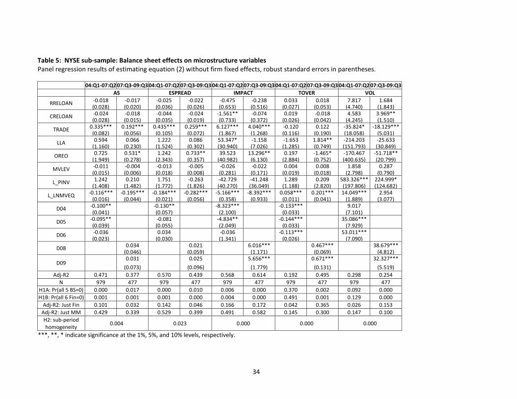
The  results  for NYSE  BHC  in  Table  5 may  be more  interesting  because  some  of  these  firms 

occupied center stage in the financial meltdown of 2008.  Starting with the joint hypotheses whose test 

  20

statistics  are  reported  at  the bottom of  Table 5, we  see  that  the  three direct opacity measures  (AS, 

ESPREAD,  IMPACT)  are  significantly  affected  by  asset  composition  in  both  sub‐  periods.   We  cannot 

reject the hypothesis (5% confidence level) that TOVER and VOL are unrelated to portfolio composition 

and  leverage  in  normal  times,  although  the  crisis‐period  results  are  consistent with  these  variables 

reflecting balance sheet composition.  All five microstructure variables show signs of being determined 

differently (in terms of the βk estimated coefficients) in the normal vs. the crisis periods. As for the NASD 

banks, the year dummies’ coefficients  indicate higher values for the first four microstructure variables 

during  the  crisis.    Surprisingly,  the  return  VOL  changes  little  between  the  two  sub‐periods  after 

controlling for asset composition. 

Turning  to  the  coefficients  on  individual  asset  shares,  we  find  little  effect  of  residential  or 

commercial  real  estate  loans  in  either  the  normal  or  the  crisis  sub‐period.      TRADE  significantly 

contributes to firm opacity, as  implied by the positive coefficients on all three  information asymmetry 

variables.  However, the coefficients on TRADE are quite similar for the two sub‐periods, suggesting that 

large  banks’  trading  accounts were  not  substantially more  difficult  for  outsiders  to  value  during  the 

crisis.    TRADE  does  not  affect  share  TOVER.    Somewhat  surprisingly,  TRADE  tends  to  reduce  return 

volatility, although this effect is smaller during the crisis period.  A higher LLA or OREO tends to reduce 

the three direct opacity measures, although these effects do not appear to be statistically significant. 

In short, the NYSE BHC results  in Table 5 broadly resemble those for the NASD BHC  in Table 4.  

Asset  composition  significantly  affects  the microstructure  variables, but  the  specific  coefficients  shift 

between  the normal and crisis sub‐periods.     Whereas NASD banks exhibited particular effects of real 

estate holdings, the NYSE banks’ most influential balance sheet category was trading accounts assets.   

 

VI.  Conclusions 

 Although many banking policy actions took place during the 2007‐09 financial crisis are predicated on 

the opacity of financial  intermediary firms, the question of bank opaqueness has not been resolved  in 

  21

the banking  literature.   We have  investigated this question using data over a twenty‐year period, with 

particular emphasis on the recent financial crisis.   In this paper, we present two lines of inquiry to assess 

whether  banking  firms  are  unusually  opaque  and  how  that  opacity might  be  determined.    First, we 

directly compare equity microstructure measures  related  to asymmetric  information or differences of 

opinion between banks and nonbanks.  The evidence indicates most clearly that large banks, traded on 

the NYSE, are not substantially more difficult  to evaluate  than  their control  (nonfinancial, peer)  firms, 

except  during  the  recent  financial  crisis.   During  “normal”  times,  the NYSE  bank  holding  companies 

exhibit  slightly higher adverse  selection  components  in  their bid‐ask  spreads, but  lower price  impact.  

Their significantly lower trading activity and return volatility suggest that these large banks do not seem 

to  be  opaque.    A  similar  conclusion  applies  to  smaller  bank  holding  companies,  traded  on  NASD.  

However, the comparisons between banks and nonbanks during the financial crisis period are strikingly 

different.    Bank  spreads’  adverse  selection  components  are  200%  to  300%  of  their  “normal  period” 

levels, and price impacts significantly exceed those of nonfinancial peer firms.  The larger (NYSE) banks 

also exhibit  significantly more volatile  returns during  the crisis, although volatility and  share  turnover 

both remain significantly lower (than peers) even during the crisis.  One distinct finding of our analysis is 

that  bank  opacity  varies  substantially  through  time.    Thus,  a  clear  implication  is  that  a  researcher’s 

ability to find evidence that banking firms are opaque depends on the sampling period examined.     

Second,  having  detected  time‐varying  bank  opaqueness, we  attempt  to  explain  opacity with 

bank asset composition.   Although we again find sharp differences on the effects of asset composition 

on our opacity measures  for  the  recent crisis period, pinning down  the source of bank opaqueness  is 

challenging.   The exact mechanism and  the  channels  through which bank opaqueness manifests  into 

market microstructure characteristics therefore remain an important area for further research. 

Regarding policy responses to the financial crisis, our empirical evidence clearly shows that bank 

opaqueness  surged during  the  crisis.   However, whether  it  is  information asymmetry or difference  in 

opinion, or both, that raise bank opacity is less clear cut.  Nevertheless, to the extent that bank opacity 

  22

contributes  to  instability, government  intervention  to  lessen  information asymmetry or disagreement, 

including  the  Supervisory  Capital Assessment  Program  to  produce  otherwise  unavailable  information 

about banks, seems appropriate to foster stability.  

   

  23

References 

Akerlof, G., 1970.  The market for ‘lemons’: Quality uncertainty and the market mechanism. Quarterly Journal of Economics 84, 488‐500. 

Amihud, Y., 2002. Illiquidity and Stock Returns: Cross‐Section and Time Series Effects, Journal of 

Financial Markets 5, 2002, 31‐56.  

Bagehot, W. (pseud.) 1971.  The only game in town. Financial Analysts Journal 27, 12‐14. 

Benston, G., Hagerman, R., 1974.  Determinants of bid‐asked spreads in the over‐the‐counter market. Journal of Financial Economics 1, 353‐364. 

Bessembinder, H.,  K. Chan, and P. Seguin.  1996. An empirical examination of inhnation, difirrences of’opinion, and trading activity,  Journal of Financial Economics 40, 105‐134 

Bessembinder, H., 2003. Trade execution costs and market quality after decimalization, Journal of Financial and Quantitative Analysis 38, 747‐777. 

Brennan, M., Subramanyam, A., 1995.  Investment analysis and price formation in securities markets. Journal of Financial Economics 38, 361‐381. 

Demsetz, H., 1968.  The cost of transacting. Quarterly Journal of Economics 82, 33‐53. 

Desai, A., Nimalendran, M., Venkataraman, S., 1998.  Changes in trading activity following stock splits and their effect on volatility and the adverse‐information component of the bid‐ask spread. Journal of Financial Research 21, 159‐183.   

Fama, Eugene F., James D. MacBeth, 1973, Risk, Return, and Equilibrium: Empirical Tests, The Journal of Political Economy 81, 607‐636.   

Flannery, M.J., S.H. Kwan and M. Nimalendran, 2004, Market evidence on the opaqueness of banking firms’ assets, Journal of Financial Economics 71, page 419‐460. 

George, T., Kaul, G., Nimalendran, M., 1991.  Estimation of the bid‐ask spread and its components: A new approach. Review of Financial Studies 4, 623‐656. 

Glosten, L., Harris, L., 1988. Estimating the components of the bid‐ask spread. Journal of Financial Economics 21, 123‐142. 

Gorton, G., Pennacchi, G., 1990.  Financial‐intermediaries and liquidity creation. Journal of Finance 45, 49‐71. Harris, M. Raviv, A., 1993.  Differences of opinion make a horse race. Review of Financial Studies 6, 473‐506.  Heider, Florian, Marie Hoerova, and Cornelia Holthausen (2010), Liquidity Hoarding and Interbank Market Spreads: The Role of Counterparty Risk, ECB working paper (June).  

Heider, Florian, Marie Hoerova, and Cornelia Holthausen, “Liquidity Hoarding and Interbank Market Spreads: The Role of Counterparty Risk,” European Central Bank working paper 1126 (December 2009). 

Huang, R., Stoll, H., 1994.   Market microstructure and stock return predictions. Review of Financial Studies 7, 179‐213. 

  24

Iannotta,  G.  (2006).  Testing  for  opaqueness  in  the  european  banking  industry:  evidence  from  bond 

credit ratings, Journal of Financial Services Research, 30, 287–309.   

Jones, C.,  Kaul, G., Lipson, M., 1994. Information, trading, and volatility. Journal of Financial Economics 36, 127‐154.  

Karpoff, J., 1987.  The relation between price changes and trading volume: A survey. Journal of Financial and Quantitative Analysis 22, 109‐126. 

Krinsky, I., Lee, J., 1996.   Earnings announcements and the components of the bid‐ask spread. Journal of Finance 51, 1523‐1535. 

Kwan, S.H., 2009, Behavior of Libor in the current financial crisis, Federal Reserve Bank of San Francisco Economic Letter 2009 issue #4. 

Kyle, A., 1985. Continuous auctions and insider trading. Econometrica 53, 1315‐1335. 

Lee, C.M.C, and Ready, M. J., 1991.  Inferring trade direction from intraday data. Journal of Finance 46, No. 2, , 733‐746. 

Lin, J., Sanger G., Booth, G., 1995.  Trade size and components of the bid‐ask spread. Review of Financial Studies 8, 1153‐1184. 

Madhavan, Ananth, 2000, Market microstructure: A survey, Journal of Financial Markets 3, 205‐258.  Morgan, D., 2002.  Rating banks:  Risk and uncertainty in an opaque industry. American Economic 

Review 92, 874‐888. 

Morgan, D., S. Peristiani, V. Savino, A. Wang, “Bank Opacity and the Informatin Value of the Stress Test,” Federal Reserve Bank of New York working paper (April 2010). 

Myers, S., Majluf, N., 1984.  Corporate investment and financing decisions when firms have iInformation that investors do not have. Journal of Financial Economics 13, 187‐222. 

Pritzker, Matthew, 2010, Informational easing: Improving credit conditions through the release of information, Federal Reserve Bank of New York Economic Policy Review, 16, 77‐88. 

Stoll, H., 1978.  The supply of dealer services in securities markets. Journal of Finance 33, 1133‐1151. 

________, 1989. Inferring the components of the bid‐ask spread: Theory and empirical tests. Journal of Finance 44, 115‐134. 

 

  25

Table 1: BHC and matched firms’ monthly microstructure  variables, 1990‐1 through 2009‐9. 

_____________________________________________________________________________________ 

Panel A: Microstructure variables 

_____________________________________________________________________________________ 

The following five market microstructure measures are computed daily and then averaged over all days 

of the month.  Definitions are provided in the text.   

ASit  = average adverse selection cost of trading stock, as a percentage of the share price.  

ESPREADit = average effective spread for transactions, as a percentage of the share price.  

TOVERit = the number of shares traded, divided by the average number of shares outstanding during the 

month.     

VOLit = the annualized daily standard deviation of the continuously compounded returns between 

adjacent trades, computed using the quote midpoints.   

IMPACT  = an estimate of Kyle’s (1985) ‘λ’, which is a price impact measure. 

______________________________________________________________________________ 

Panel B: Control variables 

_____________________________________________________________________________________ 

PINVit = the inverse of the monthly average share price.  

LNMVEQit = natural log of the month average market value of common equity.

26  

Table 1 (cont’d) Panel A: Microstructure variables for NASD BHCs and Control 

                       

   Bank Holding Companies  Matched (Control) Firms  

   N   Mean Std. dev.  Min.  Max.  Median  N   Mean 

Std. dev.  Min.  Max.  Median 

AS  55,028  1.140  1.273  ‐14.86  9.443  0.884  56,561  1.002  1.278  ‐9.51  10.40  0.732 

ESPREAD  57,518  1.797  1.469  0.000  11.61  1.416  57,637  1.682  1.507  0.000  16.28  1.271 

IMPACT  55,752  22.69  20.76  0.000  367.6  17.98  55,141  25.81  21.55  0.000  279.6  21.13 

TOVER  58,657  0.161  0.273  0.000  8.954  0.081  58,657  0.595  0.907  0.000  16.84  0.290 

VOL  55,226  36.02  43.21  0.000  456.7  22.02  56,672  53.67  50.54  0.000  416.5  36.82 

PRICE  58,657  22.59  12.82  2.000  208.7  20.60  58,657  20.87  13.68  0.030  260.4  18.51 

MVEQ**  58,657  0.49  1.61  0.000  39.6  0.13  58,657  0.48  1.60  0.000  51.9  0.13 

                                       Panel B: Microstructure variables for NYSE BHCs and Control                       

   Bank Holding Companies  Matched (Control) Firms  

   N   Mean Std. dev.  Min.  Max.  Median  N   Mean 

Std. dev.  Min.  Max.  Median 

AS  14,843  0.309  0.560  ‐2.285  9.272  0.132  14,858  0.296  0.545  ‐2.494  9.524  0.131 

ESPREAD  14,969  0.614  0.768  0.030  11.606  0.313  14,968  0.600  0.767  0.029  12.437  0.310 

IMPACT  14,964  14.78  14.75  0.000  145.9  9.33  14,951  14.97  14.62  0.000  217.3  9.87 

TOVER  14,969  0.351  0.516  0.003  8.954  0.227  14,969  0.515  0.748  0.001  12.880  0.319 

VOL  14,904  62.92  55.36  0.000  374.0  40.92  14,904  71.3  59.91  0.000  470.1  49.03 

PRICE  14,969  34.73  32.22  2.010  554.2  28.23  14,969  33.72  30.86  0.140  576.8  27.89 

MVEQ**  14,969  9.78  25.68  0.010  268.7  1.68  14,969  9.48  25.13  0.000  327.0  1.66 

** reported in millions of dollars                               

27  

TABLE 2: Differences in microstructure characteristics of BHCs vs. control firms   

Regression estimates of equation (1):   μ  , where denotes the jth (j = AS, ESPREAD, TOVER, 

VOL, IMPACT) BHC i’s market microstructure value in month t less that of its matching nonfinancial firm; Δ   = the inverse of the average share 

price for BHC i in month t less that of its control firm; Δ   = the log of BHC i’s average equity market value in month t less that of its control firm.  All regressions are run with robust standard errors, clustered by firm. *, **, *** indicates statistical significance at the 10%, 5%, or 1% confidence level respectively.  Panel A: Estimates from all SAMPLE months, 1990‐1 through 2009‐9 (234 months) 

  NASD Firms  NYSE Firms   AS  ESPREAD  IMPACT  TOVER  VOL  AS  ESPREAD  IMPACT  TOVER  VOL 

Intercept  0.181***  0.192***  ‐2.756***  ‐0.433***  ‐16.871***  0.026**  0.039**  0.041  ‐0.164***  ‐7.690***   (0.016)  (0.021)  (0.259)  (0.012)  (0.490)  (0.010)  (0.015)  (0.331)  (0.025)  (1.228) 

ΔPINV  2.097***  3.391***  20.310*** 0.370**  103.325***  1.866***  3.144***  ‐6.544  0.705  158.276***  (0.317)  (0.363)  (4.541)  (0.167)  (10.20)  (0.524)  (0.572)  (10.45)  (0.834)  (51.65) 

ΔLNMVEQ  ‐0.442***  ‐0.664***  ‐4.424***  0.174***  2.707**  ‐0.156***  ‐0.291***  ‐5.965***  0.065  ‐3.842   (0.034)  (0.046)  (0.496)  (0.030)  (1.303)  (0.033)  (0.045)  (1.440)  (0.060)  (3.197) 

R‐squared   0.078  0.120  0.023  0.007  0.025  0.102  0.187  0.043  0.001  0.026 N  53,987  56,993  55,142  59,184  54,294  14,744  14,968  14,951  14,975  14,843 

Panel B: Estimates from 1990‐1 through 1992‐12 (36 months) 

  NASD Firms  NYSE Firms   AS  ESPREAD  IMPACT  TOVER  VOL  AS  ESPREAD  IMPACT  TOVER  VOL 

Intercept  0.020  0.257***  ‐1.026  ‐0.370***  ‐17.724***  ‐0.011  ‐0.003  ‐1.437**  ‐0.002  ‐0.261   (0.034)  (0.060)  (0.957)  (0.028)  (2.126)  (0.011)  (0.010)  (0.568)  (0.030)  (1.638) 

ΔPINV  ‐2.896**  4.591***  4.262  ‐0.541**  116.065***  ‐3.083***  4.545***  ‐42.713  0.049  146.996**   (1.162)  (1.286)  (18.89)  (0.253)  (40.15)  (0.327)  (0.724)  (40.36)  (0.505)  (61.51) 

ΔLNMVEQ  0.364***  ‐0.902***  ‐13.241*** 0.113*  ‐18.633**  0.049  ‐0.129  ‐10.309**  0.105  ‐5.507   (0.111)  (0.166)  (2.691)  (0.058)  (7.277)  (0.030)  (0.088)  (5.006)  (0.077)  (6.455) 

R‐squared   0.045  0.182  0.056  0.016  0.083  0.198  0.617  0.054  0.014  0.167 N  2,847  4,039  2,226  5,711  2,768  1,502  1,550  1,534  1,551  1,549 

 

  28

 Table 2 (cont’d)  Panel C: Estimates from 1998‐8 through 1998‐12 (5 months)   NASD Firms  NYSE Firms 

  AS  ESPREAD  IMPACT  TOVER  VOL  AS  ESPREAD  IMPACT  TOVER  VOL Intercept  0.315***  0.323***  ‐1.364*  ‐0.342***  ‐7.536***  0.006  0.030  1.559  ‐0.204***  ‐3.103 

  (0.064)  (0.081)  (0.715)  (0.033)  (0.844)  (0.047)  (0.063)  (1.315)  (0.058)  (2.736) ΔPINV  3.215**  3.828**  3.725  ‐0.527  63.013**  3.651**  5.589***  ‐27.167  0.483  95.556** 

  (1.349)  (1.771)  (10.53)  (0.446)  (26.49)  (1.440)  (0.605)  (16.74)  (0.632)  (45.36) ΔLNMVEQ  ‐0.537***  ‐0.720***  ‐0.603  ‐0.147  ‐3.475*  ‐0.136***  ‐0.354***  ‐6.915***  ‐0.015  ‐5.984 

  (0.119)  (0.153)  (1.094)  (0.106)  (2.001)  (0.051)  (0.051)  (1.911)  (0.088)  (4.387) R‐squared   0.107  0.113  ‐0.001  0.010  0.084  0.183  0.286  0.099  0.000  0.085 

N  1,358  1,402  1,402  1,409  1,375  406  410  410  414  406    Panel D: Estimates from 2007‐7 through 2009‐9 (27 months)    NASD Firms  NYSE Firms 

  AS  ESPREAD  IMPACT  TOVER  VOL  AS  ESPREAD  IMPACT  TOVER  VOL Intercept  0.500***  0.555***  2.516***  ‐0.396***  ‐13.004***  0.083***  0.101***  3.835***  0.112  6.631** 

  (0.051)  (0.058)  (0.839)  (0.033)  (1.972)  (0.019)  (0.026)  (1.025)  (0.141)  (3.087) ΔPINV  ‐0.243  ‐0.048  ‐13.956  3.412***  157.246*** 0.987***  1.273***  ‐18.130  2.141  49.114 

  (0.843)  (1.039)  (9.869)  (1.118)  (35.51)  (0.295)  (0.392)  (13.64)  (2.516)  (50.65) ΔLNMVEQ  ‐0.275***  ‐0.348***  ‐8.256***  0.388**  2.740  ‐0.070  ‐0.092  ‐6.323***  0.445  ‐5.251 

  (0.099)  (0.118)  (1.446)  (0.165)  (4.901)  (0.049)  (0.067)  (1.669)  (0.404)  (5.359) R‐squared   0.009  0.013  0.014  0.029  0.033  0.045  0.049  0.031  0.009  0.010 

N  6,300  6,317  6,317  6,318  6,305  1,490  1,490  1,490  1,490  1,490 

   

  29

 Table 2 (cont’d)  

Panel E: Estimates from all "normal" months, 1990‐1 through 2009‐9 (166 months)    NASD Firms  NYSE Firms 

  AS  ESPREAD  IMPACT  TOVER  VOL  AS  ESPREAD  IMPACT  TOVER  VOL Intercept  0.152***  0.148***  ‐3.659***  ‐0.452***  ‐17.847***  0.031***  0.048***  ‐0.279  ‐0.217***  ‐10.465***

  (0.015)  (0.021)  (0.254)  (0.014)  (0.456)  (0.011)  (0.017)  (0.338)  (0.019)  (1.396) ΔPINV  3.017***  4.036***  25.729*** 0.014  91.144***  3.163***  4.325***  3.545  0.346  228.468**

  (0.314)  (0.406)  (5.267)  (0.135)  (9.325)  (0.502)  (0.719)  (12.92)  (0.453)  (102.1) ΔLNMVEQ  ‐0.482***  ‐0.661***  ‐3.444***  0.177***  4.450***  ‐0.178***  ‐0.298***  ‐5.114***  0.038  ‐1.315 

  (0.036)  (0.052)  (0.564)  (0.032)  (1.273)  (0.034)  (0.052)  (1.508)  (0.050)  (4.253) R‐squared   0.127  0.140  0.024  0.010  0.022  0.165  0.213  0.037  0.001  0.027 

N  43,482  45,235  45,197  45,746  43,846  11,346  11,518  11,517  11,520  11,398   Panel F: Estimates from 1990‐1 through 1997‐12 (93 months)   NASD Firms  NYSE Firms 

  AS  ESPREAD  IMPACT  TOVER  VOL  AS  ESPREAD  IMPACT  TOVER  VOL Intercept  0.074**  0.197***  ‐1.664***  ‐0.364***  ‐10.297***  ‐0.017*  ‐0.005  ‐1.010***  ‐0.050**  ‐2.854*** 

  (0.031)  (0.047)  (0.236)  (0.017)  (0.628)  (0.009)  (0.012)  (0.341)  (0.022)  (0.985) ΔPINV  ‐0.713  5.972***  12.958*  ‐0.834***  101.179*** ‐1.033  4.884***  ‐12.042  0.176  202.862***

  (1.133)  (0.978)  (6.913)  (0.178)  (19.749)  (1.350)  (1.164)  (30.203)  (0.517)  (44.669) ΔLNMVEQ  ‐0.427***  ‐0.864***  ‐2.173***  0.055**  ‐3.689**  ‐0.132  ‐0.306*  ‐7.383*  0.005  ‐5.369** 

  (0.078)  (0.105)  (0.407)  (0.028)  (1.538)  (0.101)  (0.155)  (3.964)  (0.040)  (2.610) R‐squared   0.020  0.144  0.013  0.013  0.046  0.017  0.298  0.071  0.000  0.186 

N  10,862  13,250  11,400  15,379  10,983  3,831  3,916  3,900  3,917  3,885      

30  

 

Table 3:  Summary statistics for the financial variables included in panel regressions 

Quarterly data, 2003Q1 – 2009Q3. 

_____________________________________________________________________________________ 

Panel A: BHC financial variables 

_____________________________________________________________________________________ 

The following six balance sheet variables are measured at the end of quarter t and are deflated by the market value of equity at the end of quarter t‐1, MVEQi,t‐1:  RELOANit = total loans secured by residential real estate. 

CRELOAN = total loans secured by commercial real estate. 

LLAit = allowance for loan and lease losses. 

TRADEit = trading account assets valued at market value or the lower of cost or market.  

OREOit = other real estate owned. 

MVLEVit = sum of liabilities’ book values at the end of quarter t plus equity’s market value at the end of  

  quarter t‐1, divided by equity’s market value at t‐1. 

_____________________________________________________________________________________ 

Panel B: Microstructure variables 

_____________________________________________________________________________________ 

The market microstructure variables defined in Table 1 are summarized here on a quarterly basis for the 

period 2003Q1 – 2009Q3

31  

 Panel A: Microstructure variables for NASD BHCs and Control 

                       

   Bank Holding Companies  Matched (Control) Firms  

   N   Mean Std. dev. 

Min.  Max.  Median N   Mean Std. dev. 

Min.  Max.  Median

AS  6,875  0.996  1.088  0.014  9.036  0.643  6,806  0.776  0.975  0.009  10.29  0.441 

ESPREAD  6,875  1.340  1.288  0.043  10.41  0.982  6,807  1.092  1.202  0.036  12.76  0.708 

IMPACT  6,875  33.95  19.94  1.706  425.5  30.85  6,807  34.30  22.62  0.534  366.0  30.30 

TOVER  6,875  0.267  0.403  0.006  8.169  0.143  6,807  0.904  1.491  0.001  39.32  0.498 

VOL  6,875  64.19  52.48  5.504  464.6  45.83  6,806  87.86  55.97  0.852  569.0  71.50 

                                      Panel B: Microstructure variables for NYSE BHCs and Control                       

   Bank Holding Companies  Matched (Control) Firms  

   N   Mean Std. dev. 

Min.  Max.  Median N   Mean Std. dev. 

Min.  Max.  Median

AS  1,690  0.213  0.403  ‐0.027  4.261  0.059  1,690  0.187  0.372  ‐0.053  5.168  0.051 

ESPREAD  1,690  0.389  0.556  0.032  5.855  0.175  1,690  0.353  0.525  0.032  6.166  0.153 

IMPACT  1,690  17.25  16.61  2.155  183.4  11.58  1,690  16.30  15.70  0.908  146.9  11.00 

TOVER  1,690  0.623  0.837  0.009  11.021  0.363  1,690  0.822  1.109  0.001  13.040  0.548 

VOL  1,690  98.80  60.95  8.003  430.4  86.24  1,690  108.9  64.92  6.131  528.4  99.70 

                                                               

 

  32

Panel C: BHC financial characteristics for NASD and NYSE BHCs  

   NASD sample BHC  NYSE sample BHC 

   N   Mean Std. dev. 

Min.  Max.  Median N   Mean Std. dev. 

Min.  Max.  Median

RRELOAN  6,875  1.546  1.697  0.000  42.60  1.168  1,690  1.677  2.611  0.000  49.40  1.218 

CRELOAN  6,875  3.217  3.868  0.000  106.0  2.347  1,690  2.096  8.352  0.000  213.3  1.147 

TRADE  6,875  0.015  0.143  0.000  4.756  0.000  1,690  0.192  0.958  0.000  23.632  0.003 

LLA  6,875  0.094  0.152  0.000  2.694  0.058  1,690  0.096  0.354  0.000  8.244  0.048 

OREO  6,875  0.030  0.143  0.000  4.775  0.004  1,690  0.023  0.163  0.000  3.914  0.003 

MVEQ**  6,875  0.620  1.882  0.007  33.49  0.187  1,690  16.36  39.01  0.019  274  2.345 

MVLEV  6,875  9.020  7.267  1.324  132.0  7.121  1,690  9.003  17.907  1.077  449.380 6.615 

**MVEQ reported in billions of dollars                               

 

    

 

  33

 Table 4: NASD sub‐sample:  Balance sheet effects on microstructure variables Panel regression results of estimating equation (2) without firm fixed effects, robust standard errors in parentheses.  

 

 ***, **, * indicate significance at the 1%, 5%, and 10% levels, respectively. 

 

  04:Q1‐07:Q2 07:Q3‐09:Q3 04:Q1‐07:Q207:Q3‐09:Q304:Q1‐07:Q207:Q3‐09:Q304:Q1‐07:Q2 07:Q3‐09:Q304:Q1‐07:Q207:Q3‐09:Q3

  AS  ESPREAD  IMPACT  TOVER  VOL 

RRELOAN  ‐0.024  0.076***  ‐0.038 0.086*** ‐1.709*** ‐0.603 ‐0.023*  0.017 ‐2.315*** ‐0.304(0.026)  (0.026)  (0.029) (0.029) (0.506) (0.384) (0.012)  (0.018) (0.790) (1.051)

CRELOAN  ‐0.055***  ‐0.035*  ‐0.068*** ‐0.038* ‐1.046*** 0.106 0.027***  0.007 0.772 3.621***(0.021)  (0.020)  (0.024) (0.023) (0.403) (0.276) (0.010)  (0.015) (0.736) (0.803)

TRADE  0.013  ‐0.123  ‐0.035 ‐0.147 ‐4.807 0.888 ‐0.110*  0.208* ‐23.456*** 2.078(0.150)  (0.214)  (0.171) (0.252) (3.237) (1.832) (0.063)  (0.107) (5.717) (6.649)

LLA  ‐0.909  ‐0.778**  ‐0.913 ‐0.718 9.728 8.259 ‐0.876**  0.575 ‐14.400 28.483*(0.905)  (0.391)  (1.041) (0.450) (15.872) (5.786) (0.434)  (0.353) (29.126) (14.582)

OREO  1.294  1.124**  1.535 1.398*** 46.552* 1.433 ‐0.216 ‐0.247** 9.896 ‐4.391(1.282)  (0.442)  (1.477) (0.513) (27.651) (3.111) (0.295)  (0.101) (27.817) (9.886)

MVLEV  0.038***  0.020  0.041*** 0.015 0.242 ‐0.353* 0.009 0.008 ‐0.275 ‐1.425***(0.013)  (0.013)  (0.015) (0.015) (0.236) (0.206) (0.006)  (0.007) (0.378) (0.527)

L_PINV  0.702  ‐1.705  0.760 ‐1.890 ‐4.871 1.198 0.645**  ‐0.272 235.466*** 121.440***(1.118)  (1.148)  (1.323) (1.289) (19.051) (17.454) (0.313)  (0.618) (31.964) (41.435)

L_LNMVEQ  ‐0.409***  ‐0.916***  ‐0.519*** ‐1.096*** ‐8.311*** ‐8.816*** 0.099***  0.375*** 7.323*** 32.806***(0.027)  (0.066)  (0.032) (0.074) (0.369) (0.534) (0.008)  (0.035) (0.848) (2.755)

D04  0.154***    0.270*** 10.104*** ‐0.062***  1.894(0.028)    (0.032) (0.626) (0.013)  (2.045)

D05  0.154***    0.236*** 6.934*** ‐0.077***  ‐8.368***(0.023)    (0.027) (0.607) (0.012)  (2.203)

D06  0.059***    0.116*** 4.398*** ‐0.073***  ‐11.270***(0.018)    (0.021) (0.540) (0.010)  (2.188)

D08    0.449***  0.584*** 13.173*** 0.155*** 36.112***  (0.046)  (0.053) (0.842) (0.023) (2.331)

D09    0.250***  0.381*** 15.945*** 0.155*** 56.775***  (0.066)  (0.074) (1.469) (0.035) (3.920)

Adj‐R2  0.619  0.604  0.645  0.628  0.505  0.319  0.337  0.484  0.196  0.367 

N  3915  2039  3915  2039  3915  2039  3915  2039  3915  2039 

H1A: Pr(all 5 BS=0)  0.037  0.000  0.027  0.000  0.004  0.191  0.000  0.013  0.000  0.000 

H1B: Pr(all 6 Fin=0)  0.027  0.000  0.029  0.000  0.006  0.023  0.000  0.000  0.000  0.000 

Adj‐R2: Just Fin  0.176  0.254  0.169  0.257  0.086  0.069  0.082  0.083  0.049  0.043 

Adj‐R2: Just MM  0.603  0.567  0.625  0.589  0.444  0.246  0.294  0.384  0.123  0.260 

H2: sub‐period homogeneity 

0.000  0.000  0.000  0.000  0.000 

 

  34

 Table 5:  NYSE sub‐sample: Balance sheet effects on microstructure variables Panel regression results of estimating equation (2) without firm fixed effects, robust standard errors in parentheses.  

  04:Q1‐07:Q2 07:Q3‐09:Q3 04:Q1‐07:Q207:Q3‐09:Q304:Q1‐07:Q207:Q3‐09:Q304:Q1‐07:Q2 07:Q3‐09:Q304:Q1‐07:Q207:Q3‐09:Q3

  AS  ESPREAD  IMPACT  TOVER  VOL 

RRELOAN  ‐0.018  ‐0.017  ‐0.025 ‐0.022 ‐0.475 ‐0.238 0.033 0.018 7.817 1.684(0.028)  (0.020)  (0.036) (0.026) (0.653) (0.516) (0.027)  (0.053) (4.740) (1.843)

CRELOAN  ‐0.024  ‐0.018  ‐0.044 ‐0.024 ‐1.561** ‐0.074 0.019 ‐0.018 4.583 3.969**(0.028)  (0.015)  (0.035) (0.019) (0.733) (0.372) (0.026)  (0.042) (4.245) (1.510)

TRADE  0.335***  0.192***  0.435*** 0.259*** 6.127*** 4.040*** ‐0.120 0.122 ‐35.824* ‐18.129***(0.082)  (0.056)  (0.105) (0.072) (1.867) (1.268) (0.116)  (0.190) (18.058) (5.031)

LLA  0.594  0.066  1.222 0.086 53.347* ‐1.158 ‐1.653 1.814** ‐214.203 ‐25.633(1.160)  (0.230)  (1.524) (0.302) (30.940) (7.026) (1.285)  (0.749) (151.793) (30.849)

OREO  0.725  0.531*  1.242 0.733** 39.523 13.296** 0.197 ‐1.465* ‐170.467 ‐51.718**(1.949)  (0.278)  (2.343) (0.357) (40.982) (6.130) (2.884)  (0.752) (400.635) (20.799)

MVLEV  ‐0.011  ‐0.004  ‐0.013 ‐0.005 ‐0.026 ‐0.022 0.004 0.008 1.858 0.287(0.015)  (0.006)  (0.018) (0.008) (0.281) (0.171) (0.019)  (0.018) (2.798) (0.790)

L_PINV  1.242  0.210  1.751 ‐0.263 ‐42.729 ‐41.248 1.289 0.209 583.326*** 224.999*(1.408)  (1.482)  (1.772) (1.826) (40.270) (36.049) (1.188)  (2.820) (197.806) (124.682)

L_LNMVEQ  ‐0.116***  ‐0.195***  ‐0.184*** ‐0.282*** ‐5.166*** ‐8.392*** 0.058***  0.201*** 14.049*** 2.954(0.016)  (0.044)  (0.021) (0.056) (0.358) (0.933) (0.011)  (0.041) (1.889) (3.077)

D04  ‐0.100**    ‐0.130** ‐8.323*** ‐0.133***  9.017(0.041)    (0.057) (2.100) (0.033)  (7.101)

D05  ‐0.095**    ‐0.081 ‐4.834** ‐0.144***  35.086***(0.039)    (0.055) (2.049) (0.033)  (7.929)

D06  ‐0.036    0.034 ‐0.036 ‐0.113***  53.011***(0.023)    (0.030) (1.341) (0.026)  (7.090)

D08    0.034  0.021 6.016*** 0.467*** 38.679***  (0.046)  (0.059) (1.171) (0.069) (4.812)

D09   0.031  0.025 5.656*** 0.671*** 32.327***

  (0.073)    (0.096)    (1.779)    (0.131)    (5.519) 

Adj‐R2  0.471  0.377  0.570  0.439  0.568  0.614  0.192  0.495  0.298  0.254 

N  979  477  979  477  979  477  979  477  979  477 

H1A: Pr(all 5 BS=0)  0.000  0.017  0.000  0.010  0.006  0.000  0.370  0.002  0.092  0.000 

H1B: Pr(all 6 Fin=0)  0.001  0.001  0.001  0.000  0.004  0.000  0.491  0.001  0.129  0.000 

Adj‐R2: Just Fin  0.101  0.032  0.142  0.046  0.166  0.172  0.042  0.365  0.026  0.153 

Adj‐R2: Just MM  0.429  0.339  0.529  0.399  0.491  0.582  0.145  0.300  0.147  0.100 

H2: sub‐period homogeneity 

0.004  0.023  0.000  0.000  0.000 

 ***, **, * indicate significance at the 1%, 5%, and 10% levels, respectively.  

35  

 

 

-1

-0.5

0

0.5

1

1.5

-1

-0.5

0

0.5

1

1.5

1990 1992 1994 1996 1998 2000 2002 2004 2006 2008 2010

NASDAQ sample

Figure 1A: Intercept term from Monthly Cross Section RegressionsAS Component of Spread

-0.6

-0.4

-0.2

0

0.2

0.4

0.6

-0.6

-0.4

-0.2

0

0.2

0.4

0.6

1990 1992 1994 1996 1998 2000 2002 2004 2006 2008 2010

NYSE sample

Figure 1B: Intercept term from Monthly Cross Section RegressionsAS Component of Spread

 

  36

  

 

-1

-0.5

0

0.5

1

1.5

-1

-0.5

0

0.5

1

1.5

1990 1992 1994 1996 1998 2000 2002 2004 2006 2008 2010

NASDAQ sample

Figure 2A: Intercept term from Monthly Cross Section RegressionsEffective Spread (ESPREAD)

-0.6

-0.4

-0.2

0

0.2

0.4

0.6

-0.6

-0.4

-0.2

0

0.2

0.4

0.6

1990 1992 1994 1996 1998 2000 2002 2004 2006 2008 2010

NYSE sample

Figure 2B: Intercept term from Monthly Cross Section RegressionsEffective Spread (ESPREAD)

 

  37

-20

-10

0

10

20

-20

-10

0

10

20

1990 1992 1994 1996 1998 2000 2002 2004 2006 2008 2010

NASDAQ sample

Figure 3A: Intercept term from Monthly Cross Section RegressionsPrice Impact (IMPACT)

 

  38

 

   

-15

-10

-5

0

5

10

15

20

-15 

-10 

-5 

0

5

10 

15 

20 

1990  1992  1994  1996  1998 2000 2002 2004 2006  2008  2010

NYSE sample

Figure 3B: Intercept term from Monthly Cross Section Regressions Price Impact (IMPACT)

 

  39

  

   

-1.5

-1

-0.5

0

0.5

1

-1.5

-1

-0.5

0

0.5

1

1990 1992 1994 1996 1998 2000 2002 2004 2006 2008 2010

NASDAQ sample

Figure 4A: Intercept term from Monthly Cross Section RegressionsShare Turnover (TOVER)

-1

-0.5

0

0.5

1

1.5

-1

-0.5

0

0.5

1

1.5

1990 1992 1994 1996 1998 2000 2002 2004 2006 2008 2010

NYSE sample

Figure 4B: Intercept term from Monthly Cross Section RegressionsShare Turnover (TOVER)

 

  40

  

 

-120

-100

-80

-60

-40

-20

0

20

40

-120

-100

-80

-60

-40

-20

0

20

40

1990 1992 1994 1996 1998 2000 2002 2004 2006 2008 2010

NASDAQ sample

Figure 5A: Intercept term from Monthly Cross Section RegressionsStandard Deviation of Share Returns (VOL)

-60

-40

-20

0

20

40

60

80

-60

-40

-20

0

20

40

60

80

1990 1992 1994 1996 1998 2000 2002 2004 2006 2008 2010

NYSE sample

Figure 5B: Intercept term from Monthly Cross Section RegressionsStandard Deviation of Share Returns (VOL)