The 1999-2000 Euro-Dollar Experience: A Quantitative Approach

Laura Alfaro*

Harvard Business School

Lluis Parera-i-Ximenez**

Harvard University

June 2001

Abstract: A modified Mundell-Fleming-Dornbusch model that allows analysis of the

effect of changes in long-run output expectations on the exchange rate is used to simulate the

evolution of the euro-dollar exchange rate. This is done under two assumptions regarding

monetary policy: constant-money-supply policy and constant-price policy. We show the

dynamics that follow a change in long-run output expectations under both scenarios. Actual data

is used to calculate the change in expectations that is needed to match the euro-dollar experience.

The quantitative results show that a small change in long-run output expectations is enough to

generate the recent euro-dollar dynamics. (JEL F31, F41)

Keywords: euro, dollar, exchange rates, expectations.

We are grateful for suggestions from Alberto Alesina, Benjamin N. Friedman, N. Gregory Mankiw, Ken Rogoff and the participants in the Macroeconomics Workshop at Harvard University Economics Department. Lluis Parera-i-Ximenez would like to thank the Bank of Spain for its fellowship support. * lalfaro@hbs.edu ** lparera@kuznets.harvard.edu Harvard Business School. Morgan 263. Boston, MA 02163. U.S.A. Tel: 617-495-7981. Fax: 617-496-5985

1

1. Introduction

From its launch in January 1999 to December 2000, the euro lost about 25 percent

of its value against the US dollar. This is an interesting phenomenon not only because it

is a large depreciation but also because the European currency was, in fact, expected to

appreciate with respect to the dollar.

We can compare this recent episode to the January 1992 - December 1993

experience in Europe. During that period three European currencies, the British pound,

the Italian lira and the Spanish peseta, suffered several speculative attacks and

experienced a loss of value with respect to the German Mark of 11%, 27% and 26%,

respectively. This precipitated the breakdown of the European Monetary System1 (EMS),

the UK and Italy abandoned the EMS and the system had to be redesigned in order to

avoid further attacks on the Spanish peseta and other European currencies. Although the

92-93 episode was labeled as a crisis, we do not think that the present euro-depreciation

is one. But its loss of value is as large as it was for the troubled currencies of the EMU

and that makes the current euro-dollar experience a crisis-like situation worth looking at.

What makes the early euro-dollar experience even more interesting is the fact that

it was completely unexpected. The Bank of International Settlements wrote in their 70th

Annual Report: “the Euro’s weakness throughout the period confounded earlier general

expectations that it would trend upwards.” For the IMF2, the Euro’s performance “defied

market expectations”.

1 The EMS was a semi-floating exchange regime characterized by an upper and a lower bound, the flotation bands. 2 See IMF (1999) World Economic Outlook.

2

According to surveys conducted by Consensus Forecasts,3 at its birth in January

99, the Euro was expected to appreciate about 4.5 percent with respect to the dollar. This

error in expectations is well documented by Corsetti (2000). A quick summary of his

argument is that exchange rate expectations were off target because growth rate

expectations were wrong. The US economy was not expected to grow as fast as it did. In

particular, Consensus Forecast projected 2.3% and 3.4% growth rates in 1999 and 2000,

respectively. The Economist forecasted 2.0% in 1999 and 3.4% in the year 2000.

Actually, the US economy grew by 4.2% in 1999 and 5% in 2000.

On the other hand, Consensus Forecast expected the Euro-area to grow by 2.3%

and 2.9% during the same period; The Economist forecasted growth rates of 2.2% and

3%. In reality the Euro-area’s growth rates were 2.4% in 1999 and 3.3% in 2000.

Corsetti suggests that the higher-than-expected US growth not only explains why

exchange rates expectations were mistaken but also why the Euro depreciated so much.

However, he is not completely convinced about this last argument and finally remarks, “it

is hard to provide a convincing interpretation of the recent evolution of the Euro”.

Corsetti also stresses an interpretation of the appreciation of the dollar based on

the evolution of domestic demand in the US. According to him, “as internal demand

grows faster than supply, the real exchange needs to appreciate […]. At the same time,

the current account of the booming country goes into a deficit”.

Our goal is to follow up on Corsetti’s work and to find out how convincing the

simplest model with exchange rate dynamics can be. To the best of our knowledge, there

has been no article that tries to simulate the euro-dollar experience using an exchange rate

model and actual data. We think that this is an interesting exercise not only because it 3 These were the one-year exchange rate expectations from Consensus Forecasts in January 1999.

3

provides a formal explanation for this somewhat extraordinary evolution of these two

currencies, but also because it provides a counterpart to another view, supported by Paul

Krugman4 and Willem Duisenberg5, President of the European Central Bank (ECB),

which argues that the euro-dollar experience is a case of market irrationality and that the

evolution of the euro did not reflect the values of the fundamentals (growth, inflation and

interest rates).

Simply put, the question that we want to answer is: can we generate the

appreciation dynamics of the dollar with respect to the euro using the Mundell-Fleming-

Dornbusch (MFD) model of exchange rates and a shock in long-run output expectations?

And, if so, how large does this shock have to be to generate these dynamics?

It has been argued that the shock in long-run output expectations during this

period is the result of unprecedented improvements in Information Technology. Alan

Greenspan, chairman of the Federal Reserve Board, has expressed in several occasions

that “although it still is possible to argue that the evident increase in productivity growth

is ephemeral, I find such arguments hard to believe, and I suspect that most in this

audience would agree.”6 So, the sometimes referred as “New Economy” has generated an

increase in productivity that goes beyond the short run. This permanent productivity

change with implications for long-run output has become particularly obvious by the end

of the century. In Alan Greenspan’s own words, “four or five years into this expansion, in

the middle of the 1990’s, it was unclear whether, going forward, this cycle would differ

significantly from many others that have characterized post-World War II America. More

4 New York Times, September 20, 2000. 5 Financial Times, September 14, 2000. 6 Remarks by Chairman, October 28, 1999.

4

recently, however, it has become increasingly difficult to deny that something profoundly

different from the typical postwar business cycle has emerged.” 7

Our quantitative results show that a small change in long-run output expectations

is enough to generate the recent euro-dollar dynamics.

The paper is structured as follows. The next section presents a version of the

MFD model that allows analysis of the effect of changes in long-run output expectations

on the exchange rate. This is done under two assumptions regarding monetary policy:

constant-money-supply policy and constant-price policy. Once the model is developed,

we show the dynamics that follow a change in long-run output expectations under both

scenarios. We then proceed to perform a simulation of these dynamics using parameters

estimated from actual data to calculate the change in expectations that is needed to match

the euro-dollar experience. The last section summarizes our conclusions.

2. Mundell-Fleming-Dornbusch Model

In this section we develop a version of the MFD model that allows us to analyze

output and exchange rate dynamics after a change in long-run output expectations. The

choice of model is based on tractability. Although the MFD model has no micro

foundations, there are micro-founded versions that generate similar results8.

First we present the general framework. The system has two state (i.e., non-

jumping) variables, output and the price level. The real exchange rate is the control (i.e.,

jumping) variable, and the nominal exchange rate, which can also jump, is a function of

7 Remarks by Chairman Alan Greenpsan, January 13, 2000. 8 See Obstfeld and Rogoff (1995).

5

the previous three variables. We derive the law of motion for output, real exchange rate

and nominal exchange rate and their steady state values. Then we proceed to analyze the

effects of a change in long-run output expectations under two different assumptions

regarding monetary policy: a constant-money-supply policy and a constant-price policy.

Finally, we discuss the main differences between the two cases.

Our framework follows closely Obstfeld and Rogoff’s (1995) analysis of the

Dornbusch (1976) model. The model considers a small open economy that faces an

exogenous world interest rate i*, which is assumed constant. The domestic monetary

equilibrium is given by a standard LM curve, Mtd / Pt = f(Yt, it), of the following form:

mt – pt = - ηit+ φyt (1)

where mt ≡ log Mt is the log of the nominal money supply, pt ≡ log Pt is the log of the

domestic price level and yt ≡ log Yt is the log of domestic output. Equation (1) establishes

the traditional inverse relation between money demand and the interest rate, and the

positive relation between money demand and output9. The parameter η is the interest rate

elasticity of money demand and φ is the income elasticity of money demand.

Under the assumptions of perfect foresight, open capital markets and perfect

substitutability between foreign and domestic assets, uncovered interest parity must hold:

it = i*t + et+1 - et (2)

9 A micro-founded money demand function can be derived using money in the utility function or money in advance assumptions as in Stockman (1980) and Lucas (1982), respectively.

6

where it ≈ log (1 + it) is the domestic interest rate; i*t ≈ log (1 + i*t+1) is the world interest

rate, and et ≡ log Et is the log of the nominal exchange rate10. Equation (2) states that,

given a positive (negative) difference in the interest rate, people must expect an

appreciation (depreciation) to hold assets from both countries.

Let dty denote home output demand. To clear the goods market, we follow the

standard assumption that output is demand-determined.11 In addition, we assume that

home output is an increasing function of the real exchange rate,12

( )*dt t t ty y e p p qδ= + + − − , δ > 0 (3)

where y is the expectation of the long-run level of output and δ the elasticity of output

demand to real depreciation . If we define q as the real exchange rate,

qt ≡ et + p*t - pt (4)

then q represents the equilibrium exchange rate consistent with full employment.

As expressed in Obstfeld and Rogoff (1996), there are different ways to justify the

inclusion of the real exchange rate in equation (3). The most intuitive one is that a real

depreciation stimulates foreign demand and, hence, raises output. A similar way to

10 Equation (2) is derived from (1+ it) = (1+ i*t) Expt[Et+1] / Et (2). Taking logs, (2) would be approximately equal to it ≈ i*t + Expt[et+1]- et , the difference accounted by Jensen’s inequality: log (Expt[Et+1]) > Expt [log(Et+1)]. 11 Obstfeld and Rogoff’s (1995) monopolistic competition model provides micro foundations for these assumptions. 12 See Obstfeld and Rogoff (1996) for a discussion on this assumption and Obstfeld and Rogoff (2000) for a discussion on the evidence.

7

interpret equation (3) is that output is determined by domestic and foreign demand and

that both are stimulated by potential output. In addition, foreign demand is an increasing

function of the real exchange rate.

The original Dornbusch (1976) model has not generally been used to explore the

effects of changes in expected long-run output y . Since our main motivation is precisely

to understand how the exchange rate responds to changes in growth expectations, output

dynamics become a relevant part of our analysis. To capture these dynamics we follow

Blanchard’s (1981) specification of output adjustment over time, which states that output

converges to output demand according to:

( )1 , 0 1dt t ty y yγ γ+ = − ≤ ≤! (5)

where the parameter γ measures the response of output to deviations from domestic

demand.

By substituting dty , equation (3), in expression (5), we rewrite output dynamics as:

( ) ( )*1t t t t ty y y e p p qγ γδ+∆ = − − + + − −

(6)

where output grows whenever demand is stimulated, either by an increase in long-run

output expectations or by a real depreciation.

Additionally, we assume that output cannot immediately jump in response to an

expectations update. Instead, it starts to grow to its new equilibrium. In other words, in

8

the short run output is fixed. The intuition behind this assumption is that in the short run,

due to investment costs or time-to-build, output cannot react instantaneously.

Notice that, under this assumption, an increase in long-run output expectations,

'y y> , generates a crowding out of foreign demand due to an increase in domestic

demand.

To capture the stylized fact that prices tend to adjust more slowly than exchange

rates,13 the model assumes that the price level p is fixed in the short run and adjusts

slowly to changes in excess demand or supply. Price dynamics follow an inflation-

expectations-augmented Phillips curve:

( )1 1d

t t t t tp p y y p pψ+ +− = − + −" " (7)

where tp" is the price level that would have prevailed if markets had cleared, in other

words, the equilibrium price level,

*t t tp e p q≡ + −" (8)

The first term in the right-hand side of equation (7) is the effect on inflation of

deviations from long-run output or excess demand and the parameter ψ is the inverse of

the sacrifice ratio. The second part of equation (7) accounts for inflation expectations due

to “fundamentals”. This last term is the inflation “needed to keep up with expected

inflation or productivity growth; that is, the movement in prices that would be needed to 13 Obstfeld and Rogoff (1996), pages 607 and 611.

9

keep y y= if the market output were in equilibrium.”14 Simply put, this last term is the

expected rate of inflation in the expectations-augmented Phillips curve.

Substituting (8) in (7) and imposing the assumptions that the foreign price level

p* and the equilibrium real exchange rate q are constant, we obtain

( )1 1d

t t t t tp p y y e eψ+ +− = − + − (9)

Equation (9) has the same intuition as equation (7), but in (9) expected inflation is

captured by expected depreciation since it leads to higher prices for tradable goods and

thus higher inflation.

To solve the model, we combine equations (4), (9) and the simplifying

assumption p*t = p*

t+1 = 0 to obtain the law of motion for the real exchange rate q.

( )1 1t t t tq q q y yψ+ +∆ = − = − − (10)

The intuition behind equation (10) is that the real exchange rate converges to its

steady state level as output reaches its own equilibrium. In other words, as output grows

there is less crowding out of foreign demand so the real exchange rate depreciates.

Plugging (2) and (4) into (1) and assuming i* = 0 we obtain the law of motion for

the nominal exchange rate,

14 See Mussa (1984) for further discussion.

10

1 1t t t

t t t te q me e e yφη η η η+ +∆ = − = − − + (11)

As can be seen in equation (11), the dynamic behavior of the nominal exchange

rate is quite complicated. It depends on the current nominal exchange rate, the current

real exchange rate and the current level of output. The intuition behind equation (11) is

easier to see when we compute the steady-state nominal exchange rate and, later on,

when we use it to derive its saddle-path under our two different policy assumptions.

The conditions ∆qt+1 = 0 and ∆et+1 = 0, and ∆yt+1 = 0 determine the steady state

values of output, real and nominal exchange rates:

y y= (6’)

q = q (10’)

e m q yφ= + − (11’)

In the steady state, both output and the real exchange rate are equal to their long-

run levels y and q .

Whether the nominal exchange rate returns to its initial value depends on our

assumption regarding monetary policy. Under a constant-money-supply policy, the

exchange rate stays permanently appreciated after an increase in long-run output.

Conversely, other things equal, increases in the money supply generate a permanent

depreciation. The following sections analyze these points in detail.

11

2.a. Unexpected Increase in Output under a Constant-Money-Supply Policy.

We first consider a change in long-run output expectations from y to y ’ under a

constant-money-supply policy. In the new steady state, the nominal exchange rate

appreciates and prices fall. The equilibrium real exchange rate, which is exogenous in

this model, does not change. So, the new steady state is characterized by:

'y y=

q = q

'e m q yφ= + −

p = m - φ 'y

Combining the law of motion for the real exchange rate qt and the nominal

exchange rate et, equations (10) and (11) respectively, the law of motion of output,

equation (6), and the constant-money-supply assumption, we obtain the saddle-path

equation for the nominal exchange rate et. Appendix 1 provides a detailed derivation of

this result.

( )( )

( ) ( )1

1 1( )1 1 1 1

s t

t t ts t

e m y q q q yφδ φ ψη ηφ φ

δψη η γ δψη η

−∞

+=

− + = − + + − + ∆ + + + +

∑ (12)

Notice that, for a given path of output, the evolution of the nominal exchange rate

depends on (1 - φδ). If (1 - φδ) > 0, the exchange rate overshoots its long-run level in

12

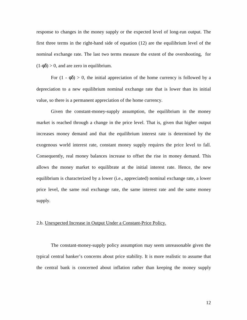
response to changes in the money supply or the expected level of long-run output. The

first three terms in the right-hand side of equation (12) are the equilibrium level of the

nominal exchange rate. The last two terms measure the extent of the overshooting, for

(1-φδ) > 0, and are zero in equilibrium.

For (1 - φδ) > 0, the initial appreciation of the home currency is followed by a

depreciation to a new equilibrium nominal exchange rate that is lower than its initial

value, so there is a permanent appreciation of the home currency.

Given the constant-money-supply assumption, the equilibrium in the money

market is reached through a change in the price level. That is, given that higher output

increases money demand and that the equilibrium interest rate is determined by the

exogenous world interest rate, constant money supply requires the price level to fall.

Consequently, real money balances increase to offset the rise in money demand. This

allows the money market to equilibrate at the initial interest rate. Hence, the new

equilibrium is characterized by a lower (i.e., appreciated) nominal exchange rate, a lower

price level, the same real exchange rate, the same interest rate and the same money

supply.

2.b. Unexpected Increase in Output Under a Constant-Price Policy.

The constant-money-supply policy assumption may seem unreasonable given the

typical central banker’s concerns about price stability. It is more realistic to assume that

the central bank is concerned about inflation rather than keeping the money supply

13

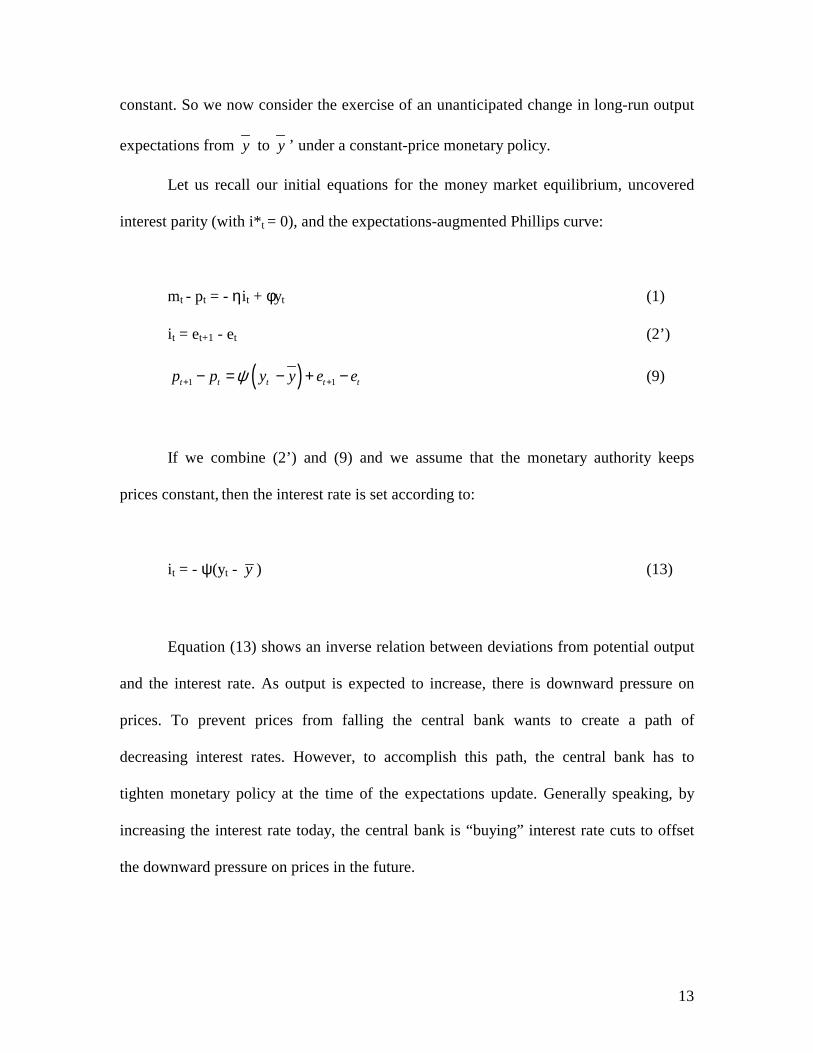
constant. So we now consider the exercise of an unanticipated change in long-run output

expectations from y to y ’ under a constant-price monetary policy.

Let us recall our initial equations for the money market equilibrium, uncovered

interest parity (with i*t = 0), and the expectations-augmented Phillips curve:

mt - pt = - ηit + φyt (1)

it = et+1 - et (2’)

( )1 1t t t t tp p y y e eψ+ +− = − + − (9)

If we combine (2’) and (9) and we assume that the monetary authority keeps

prices constant, then the interest rate is set according to:

it = - ψ(yt - y ) (13)

Equation (13) shows an inverse relation between deviations from potential output

and the interest rate. As output is expected to increase, there is downward pressure on

prices. To prevent prices from falling the central bank wants to create a path of

decreasing interest rates. However, to accomplish this path, the central bank has to

tighten monetary policy at the time of the expectations update. Generally speaking, by

increasing the interest rate today, the central bank is “buying” interest rate cuts to offset

the downward pressure on prices in the future.

14

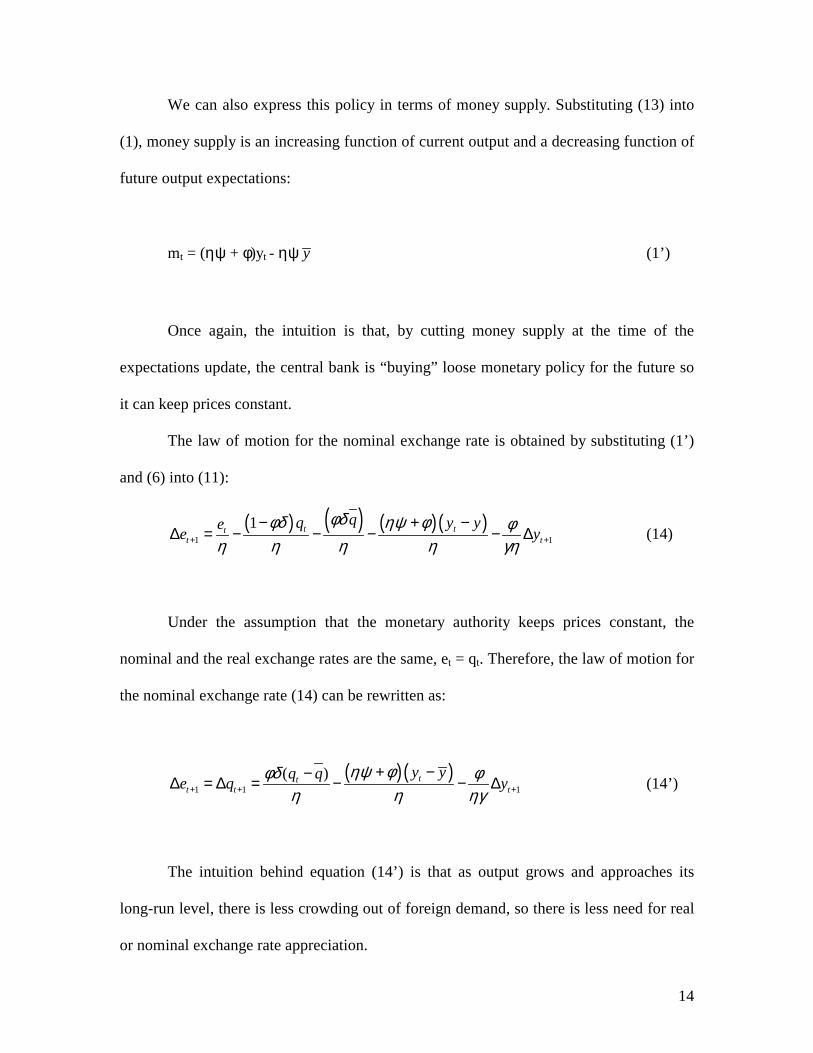
We can also express this policy in terms of money supply. Substituting (13) into

(1), money supply is an increasing function of current output and a decreasing function of

future output expectations:

mt = (ηψ + φ)yt - ηψ y (1’)

Once again, the intuition is that, by cutting money supply at the time of the

expectations update, the central bank is “buying” loose monetary policy for the future so

it can keep prices constant.

The law of motion for the nominal exchange rate is obtained by substituting (1’)

and (6) into (11):

( ) ( ) ( ) ( )1 1

1 t ttt t

qq y yee yφδφδ ηψ φ φ

η η η η γη+ +

− + −∆ = − − − − ∆ (14)

Under the assumption that the monetary authority keeps prices constant, the

nominal and the real exchange rates are the same, et = qt. Therefore, the law of motion for

the nominal exchange rate (14) can be rewritten as:

( ) ( )1 1 1

( ) ttt t t

y yq qe q yηψ φφδ φ

η η ηγ+ + +

+ −−∆ = ∆ = − − ∆

(14’)

The intuition behind equation (14’) is that as output grows and approaches its

long-run level, there is less crowding out of foreign demand, so there is less need for real

or nominal exchange rate appreciation.

15

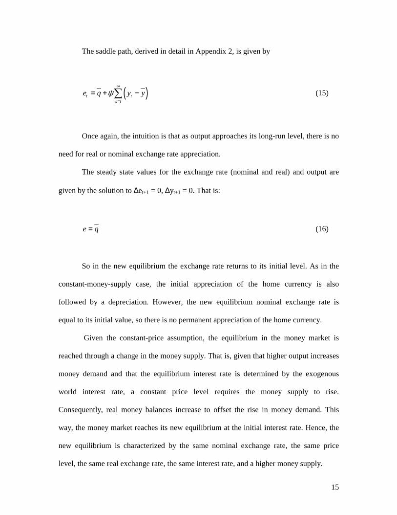
The saddle path, derived in detail in Appendix 2, is given by

( )t ts t

e q y yψ∞

=

= + −∑ (15)

Once again, the intuition is that as output approaches its long-run level, there is no

need for real or nominal exchange rate appreciation.

The steady state values for the exchange rate (nominal and real) and output are

given by the solution to ∆et+1 = 0, ∆yt+1 = 0. That is:

e q= (16)

So in the new equilibrium the exchange rate returns to its initial level. As in the

constant-money-supply case, the initial appreciation of the home currency is also

followed by a depreciation. However, the new equilibrium nominal exchange rate is

equal to its initial value, so there is no permanent appreciation of the home currency.

Given the constant-price assumption, the equilibrium in the money market is

reached through a change in the money supply. That is, given that higher output increases

money demand and that the equilibrium interest rate is determined by the exogenous

world interest rate, a constant price level requires the money supply to rise.

Consequently, real money balances increase to offset the rise in money demand. This

way, the money market reaches its new equilibrium at the initial interest rate. Hence, the

new equilibrium is characterized by the same nominal exchange rate, the same price

level, the same real exchange rate, the same interest rate, and a higher money supply.

16

2.c. Constant-Money-Supply vs. Constant Prices:

Our two monetary policy assumptions generate an initial appreciation of the home

currency followed by a depreciation, so they both generate overshooting dynamics. In the

constant-money-supply case, the nominal exchange rate is permanently lower (i.e.,

appreciated) in equilibrium while in the constant-price case it reverts to its initial value.

The main difference between the two cases is the behavior of the money market.

While in the constant-money-supply case the money market is equilibrated through a

decrease in the price level, in the constant-price case the equilibrium is reached because

of an increase in the money supply.

3. Quantitative Analysis

In the previous section we develop a version of the MFD model that allows for

changes in expected long-run output. We use this model to show that a positive shock in

long-run output expectations leads to an appreciation of the home currency under both a

constant-money-supply policy and a constant-price policy.

In both cases the initial change in the nominal exchange rate is equal to the initial

change in the real exchange rate because we assume that the price level is fixed in the

short run. As we discussed in the previous section, a change in long-run output

expectations generates a real appreciation because we assume that output is also slow to

adjust to its new equilibrium. In other words, we do not allow output to jump in response

to a change in long-run output expectations, so the increase in domestic demand that

17

higher long-run output expectations generate is offset by a decrease in foreign demand

(i.e., an increase in the trade balance deficit). This crowding out of foreign demand takes

the form of a real appreciation that also generates an equivalent nominal appreciation in

the short run.

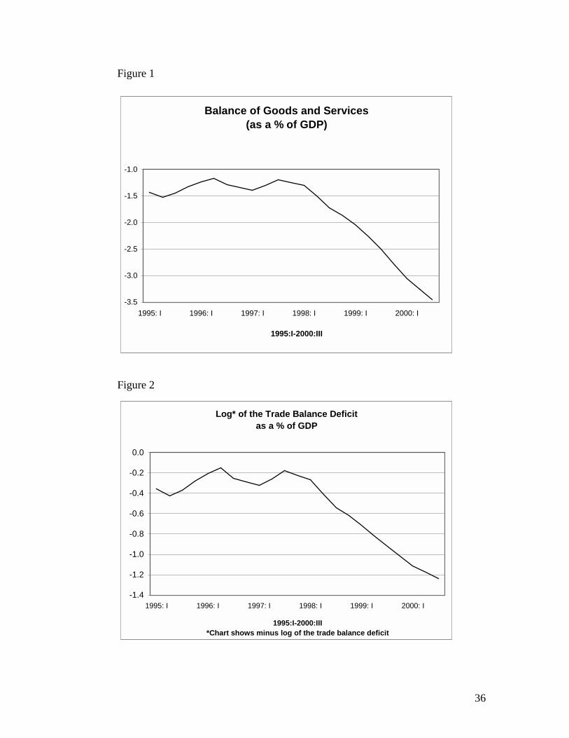
Even though the focus of our research is on the exchange rate impact of a change

in long-run output expectations, the impact on the trade balance is a relevant part of our

analysis. Figures 1 and 2 show the recent evolution of the US trade balance deficit, using

quarterly data. Figure 1 shows the evolution of the trade balance deficit as a percentage of

GDP. The increase in the trade deficit started in 1998 and continued during 1999 and

2000. At the beginning of 1999 the trade balance deficit was 2 percent of GDP and about

3.5 percent of GDP at the end of 2000. Figure 2 shows the same data in logarithms. Here

we can see that the trade balance deficit increased about 62 percent during the period of

interest. This evidence on the increase in the US trade balance deficit supports our

model’s implication that higher domestic demand generated a crowding out of foreign

demand.

The goal of our paper is to provide a quantitative idea of how large the change in

long-run output expectations has to be to generate an initial appreciation that matches the

recent euro-dollar experience. To do this, we evaluate our model with a variety of

parameter values and compute the change in output expectations that generates an initial

appreciation of 25 percent, which is the extent of the appreciation of the dollar with

respect to the euro. For each combination of parameters we provide the percentage

change in long-run output and the dynamics that follow that change under our two

different policy assumptions.

18

It is easy to find in the literature some “consensus” estimates of three of the five

parameters that we need, the inverse of the sacrifice ratio ψ , the income elasticity of

money demand φ , and the interest rate elasticity of money demand η .

The textbook number for the inverse of the sacrifice ratio ψ , which comes from

Gordon and King’s (1982) paper, is 15

15 However, there are a variety of estimates in the

literature that we will also consider in our exercise. Gordon (1997) provides an estimate

of 13 and Staiger, Stock and Watson’s (1996) paper reports small, but statistically

significant, numbers in the range 18 to 1

4 .

For the income elasticity of money demand φ and the interest rate elasticity of

money demand η we find a large consensus in the literature represented by Hoffman and

Rasche (1991), Lucas (1988), Mankiw and Summers (1986) and Stock and Watson

(1993). The estimates in all these articles are 1 and 0.1 for the income and interest rate

elasticities, respectively.

Since we have not been able to find a number for the elasticity of output demand

to real depreciation δ , we perform a variety of estimations using different data sets and

time periods with an ordinary least squares (OLS) regression for the logarithm of US real

GDP on the logarithm of the US real exchange rate.

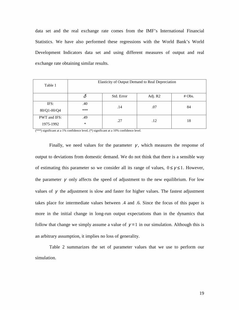
Table 1 shows the OLS results for the elasticity of output demand to real

depreciation δ . The first row presents an estimate based on quarterly data from the

IMF’s International Financial Statistics from 80/Q1 to 00/Q4. The estimate in the second

row uses yearly data from 1975 to 1992. Real GDP comes from the Penn World Table

15 See Mankiw 2000, page 371.

19

data set and the real exchange rate comes from the IMF’s International Financial

Statistics. We have also performed these regressions with the World Bank’s World

Development Indicators data set and using different measures of output and real

exchange rate obtaining similar results.

Table 1 Elasticity of Output Demand to Real Depreciation

δ Std. Error Adj. R2 # Obs.

IFS:

80/Q1-00/Q4

.40

*** .14 .07 84

PWT and IFS:

1975-1992

.49

* .27 .12 18

(***) significant at a 1% confidence level, (*) significant at a 10% confidence level.

Finally, we need values for the parameter γ , which measures the response of

output to deviations from domestic demand. We do not think that there is a sensible way

of estimating this parameter so we consider all its range of values, 0 1γ≤ ≤ . However,

the parameter γ only affects the speed of adjustment to the new equilibrium. For low

values of γ the adjustment is slow and faster for higher values. The fastest adjustment

takes place for intermediate values between .4 and .6. Since the focus of this paper is

more in the initial change in long-run output expectations than in the dynamics that

follow that change we simply assume a value of 1γ = in our simulation. Although this is

an arbitrary assumption, it implies no loss of generality.

Table 2 summarizes the set of parameter values that we use to perform our

simulation.

20

Table 2 Inverse of the sacrifice ratio

Income elasticity of

money demand

Interest rate elasticity of

money demand

Elasticity of output demand to real depreciation

Response of output to

deviations from domestic demand

Parameters ψ φ η δ γ

Values 18 , 1

5 , 14 , 1

3 1 .1 .40, .49 1γ =

3.a. Constant-Money-Supply Case:

To perform our simulation we need some initial values for the different variables

so, in the initial equilibrium, we assume:

0 0y y= =

0 0q q= =

These initial values and equations (6) and (10) imply that both output and the real

exchange rate are constant in equilibrium. That is:

0 0y =!

0 0q =!

We also assume that, at first, the domestic price level is zero:

0 0p =

21

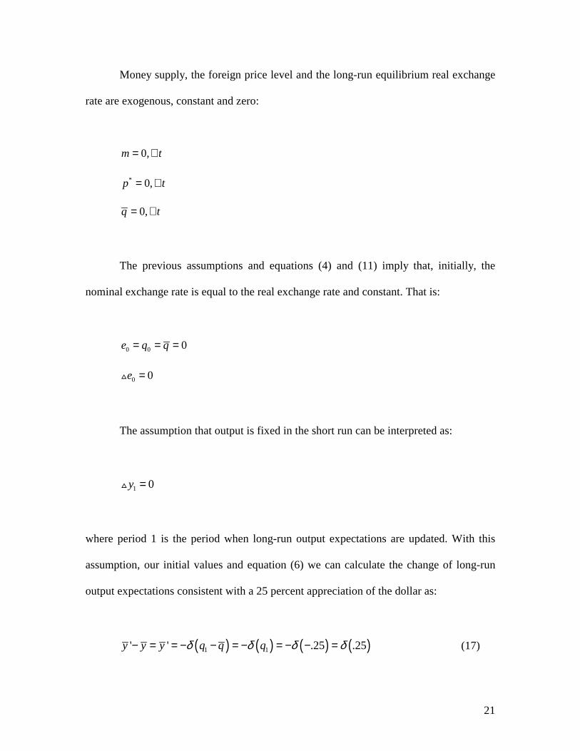
Money supply, the foreign price level and the long-run equilibrium real exchange

rate are exogenous, constant and zero:

0,m t= ∀

* 0,p t= ∀

0,q t= ∀

The previous assumptions and equations (4) and (11) imply that, initially, the

nominal exchange rate is equal to the real exchange rate and constant. That is:

0 0 0e q q= = =

0 0e =!

The assumption that output is fixed in the short run can be interpreted as:

1 0y =!

where period 1 is the period when long-run output expectations are updated. With this

assumption, our initial values and equation (6) we can calculate the change of long-run

output expectations consistent with a 25 percent appreciation of the dollar as:

( ) ( ) ( ) ( )1 1' ' .25 .25y y y q q qδ δ δ δ− = = − − = − = − − = (17)

22

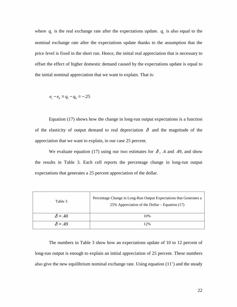
where 1q is the real exchange rate after the expectations update. 1q is also equal to the

nominal exchange rate after the expectations update thanks to the assumption that the

price level is fixed in the short run. Hence, the initial real appreciation that is necessary to

offset the effect of higher domestic demand caused by the expectations update is equal to

the initial nominal appreciation that we want to explain. That is:

1 0 1 0 .25e e q q− = − = −

Equation (17) shows how the change in long-run output expectations is a function

of the elasticity of output demand to real depreciation δ and the magnitude of the

appreciation that we want to explain, in our case 25 percent.

We evaluate equation (17) using our two estimates for δ , .4 and .49, and show

the results in Table 3. Each cell reports the percentage change in long-run output

expectations that generates a 25 percent appreciation of the dollar.

Table 3 Percentage Change in Long-Run Output Expectations that Generates a

25% Appreciation of the Dollar – Equation (17)

.40δ = 10%

.49δ = 12%

The numbers in Table 3 show how an expectations update of 10 to 12 percent of

long-run output is enough to explain an initial appreciation of 25 percent. These numbers

also give the new equilibrium nominal exchange rate. Using equation (11’) and the steady

23

state conditions of the other variables, the new equilibrium nominal exchange rate is

given by:

* 'e q m yφ= + − (18)

So, under our assumptions for the values of q and m and taking the value of the income

elasticity of money demand 1φ = , the change in the equilibrium nominal exchange rate is

equal to the change in long-run output. In our case, the nominal exchange rate appreciates

between 10 to 12 percent in the new equilibrium. It is clear from equation (18) that an

equilibrium nominal appreciation critically depends on the constant-money-supply

assumption.

We can compute the dynamics for output and the real exchange rate that follow

the change in long-run output expectations using equations (6) and (10). We only need

these two equations because the dynamics for output and the real exchange rate do not

depend on the nominal exchange rate. On the other hand, the dynamics of the nominal

exchange rate depend on output, the real exchange rate and the nominal exchange rate.

So, once we have the dynamics for output and the real exchange rate, we can get the

dynamics for the nominal exchange rate using the saddle path for the nominal exchange

rate, equation (12).

To compute the dynamics of output and the real exchange rate we proceed as

follows:

1) We take a 25% real appreciation as our starting point.

24

2) Using equation (17) we compute the change in long-run output expectations

that is consistent with a 25% real appreciation.

3) We do not allow output to change in the period when expectations are updated

so 1 0y =! . This implies 2 1y y= .

4) Using equation (10) we compute the change in the real exchange rate, 1q! ,

which allows us to compute 2q .

5) Using equation (6) we compute the change in output, 2y! , which allows us to

compute 3y .

6) We keep iterating equations (6) and (10) until the new equilibrium is reached.

We consider that the new equilibrium is reached when both output and the

real exchange rate reach their equilibrium levels up to the first three decimal

numbers.

Once we have the values of output and the real exchange rate from the first period

to the new equilibrium, we can use the saddle path for the nominal exchange rate,

equation (12), to compute the values of the nominal exchange rate.

Table 4 shows the results of computing these dynamics using all the different

parameter values that are reported in Table 2. For each combination of parameter values

we report the number of years it takes for the new equilibrium to be reached and the

average growth rate of output during those years.

25

Output Dynamics - Equations (6) and (10) Using Steps 1) to 6)

.40δ = , 1φ = , .1η = , 1γ = Change in Long-Run Output Expectations of 10%

Long-Run Nominal Exchange Rate Appreciation of 10%

Table 4

Years to New Equilibrium Average Growth Rate of Output 1

3ψ = 34 .3%

14ψ = 48 .2%

15ψ = 62 .2%

18ψ = 104 .1%

.49δ = , 1φ = , .1η = , 1γ = Change in Long-Run Output Expectations of 12%

Long-Run Nominal Exchange Rate Appreciation of 12%

Years to New Equilibrium Average Growth Rate of Output 1

3ψ = 26 .5%

14ψ = 38 .3%

15ψ = 49 .2%

18ψ = 85 .1%

The average growth rate of output has to be interpreted as additional to the growth

rate that had already been expected. For instance, if people expected the US to grow at an

average growth rate of 2% for the following 50 years, they update their expectations to an

average growth rate of 2.2%, assuming .40δ = and 14ψ = .

The results are very similar for the two values of δ and they react to different

values of the inverse of the sacrifice ratio in the same way. A higher sacrifice ratio

increases the time it takes to reach the new equilibrium and, for a given increase in long-

run output, decreases the average growth rate.

However, most of the adjustment takes place during the first years after the

change in expectations. We exemplify this point with a more detailed description of the

26

dynamics in the case when .40δ = and 14ψ = . In this case the new equilibrium is

reached in 48 years with an average growth rate of .2% per year. However, the average

growth rate during the first ten years is .7% per year, .4% during the first 20 years, and

.3% during the first 30 years.

Most of the adjustment is concentrated at the beginning. In fact, after 20 years

output is at .088, which is very close to the equilibrium level of .1. The real exchange rate

after 20 years is -.02 and the nominal exchange rate is -.11, both close to their

equilibrium levels of 0 and -.1, respectively.

Figure 3 shows the evolution of output, the real exchange rate and the nominal

exchange rate. The nominal exchange rate comes from equation (12) and the values of

output and the real exchange rate from equations (6) and (10) following steps 1) to 6).

Clearly, the adjustment to the new equilibrium is faster for all variables during the initial

periods.

3.b. Constant-Price Case:

We perform the simulation for the constant-price case using the same initial

values as in the constant-money-supply case with the difference that, in the present case,

the price level that is constant over time and money supply is allowed to change. That is:

0 0m =

0 0,p p t= = ∀

27

As discussed in the theory section, the only differences between these two cases

are that, in the constant-price case:

1) The nominal and the real exchange rate are the same. They have the same

evolution and converge to their initial value of zero.

2) The equilibrium in the money market is reached through a change in the money

supply.

As in the previous case, output dynamics determine the real exchange dynamics,

which, in this case, are also the nominal exchange rate dynamics. The driving force

behind these dynamics is the crowding out effect that domestic demand has on foreign

demand. This effect depends critically on the assumption that output cannot jump in the

period when expectations are updated, so the increase in domestic demand generated by

higher long-run output expectations is offset by an equivalent decrease in foreign

demand. Such decrease in foreign demand takes the form of a real exchange rate

appreciation of the dollar.

To compute output and exchange rate dynamics we can use the law of motion for

output, equation (6), and the new law of motion for the exchange rate, equation (14).

These new exchange rate dynamics incorporate the constant-price monetary policy

assumption, equation (1’), and the fact that under constant prices the real and the nominal

exchange rate are the same. Following the same steps 1) to 6) described in the constant-

money-supply case and equations (6) and (14), we compute output and exchange rate

dynamics for the constant-price case.

Another way to generate the exchange rate dynamics is to use the new saddle-path

equation for the exchange rate, equation (15), and the path of output that we calculate

28

with equations (6) and (14). The results are the same showing that the model is internally

consistent.

Since the driving force behind output and exchange rate dynamics is the same as

in the constant-money case, it is not surprising that the results are also the same. The

evolution of output and the real exchange rate is exactly the same as in the previous case.

And, since nominal and real exchange rates are equivalent under the constant-price

policy, the dynamics of the nominal exchange rate are now the same as the dynamics we

previously reported for the real exchange rate. Once again, depending on the value of the

elasticity of output to real depreciation δ , the change in long-run output expectations that

generates an initial appreciation of the dollar of a 25 percent is between 10 and 12

percent. The effect of changing the combination of parameters on the evolution of output

is the same as reported in Table 4.

Figure 4 shows the evolution of output and the exchange rate (real and nominal)

after the change in long-run output expectations assuming .40δ = and 14ψ = .

3.c. Constant-Money-Supply vs. Constant-Price:

As we discussed before, the main difference between the constant-money case

and the constant-price case is the behavior of the money market. Since we already have

the values of output, the real exchange rate, and the nominal exchange rate under both

assumptions, we can also compute the evolution of the money supply, prices, and the

interest rate in both cases. We do so assuming .40δ = and 14ψ = .

29

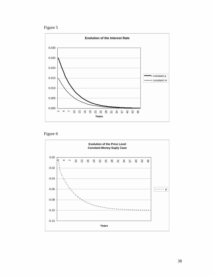
Figure 5 shows the evolution of the interest rate under our two different monetary

policy assumptions calculated from the interest rate parity condition, equation (2). In both

cases the interest rate initially jumps to a higher-than-equilibrium level and then

converges to its original value. The initial jump is due to the depreciation path that

follows the appreciation of the dollar generated by the expectations update and is also

given by the interest rate parity condition, equation (2). Although the equilibrium is the

same in both cases, in the constant-money-supply case the initial increase in the interest

rate is smaller. This happens because in this case the nominal exchange rate does not

depreciate as much as in the constant-price case, where nominal depreciation has to

completely offset any pressure on the price level.

Figure 6 shows the evolution of the price level in the constant-money-supply case

calculated from the expectations-augmented Phillips curve, equation (9). In the period

when expectations are updated, the price level does not change because it is assumed that

it is fixed in the short run. As output and the nominal exchange rate converge to their new

equilibrium levels, the interest rate also converges to its initial value. So, given the

assumption that the money supply is constant and that money demand increases with

output, the increase in real money balances that is needed to equilibrate the money

market is achieved through a fall in the price level. In the new equilibrium, the price level

is 10 percent lower than in the initial equilibrium.

Finally, Figure 7 shows the evolution of money supply under the constant-price

assumption calculated from the monetary policy rule, equation (1’). The intuition is very

similar to the previous case. As output and the nominal exchange rate converge to their

new equilibrium levels, the interest rate also converges to its initial value. So, given the

30

assumption that the price level is constant and that money demand increases with output,

the increase in real money balances that is needed to equilibrate the money market is

achieved through an increase in the money supply. In the new equilibrium, the money

supply is 10 percent higher than in the initial equilibrium.

4. Conclusions

A modified version of the Mundell-Fleming-Dornbusch model allows us to

analyze the exchange rate impact of an increase in long-run output expectations. We

simulate this model with parameter values estimated from actual data and show that an

increase in long-run output expectations of between 10 and 12 percent is enough to

generate a 25 percent appreciation of the dollar with respect to the new European

currency. Depending on parameter values, this increase in long-run output expectations is

equivalent to between .1 and .5 percent of higher-than-expected growth during the years

that follow the expectations update.

These results suggest that the recent euro-dollar experience does not call for

assumptions of irrationality since it can be explained with a standard and plausible model.

31

Appendix 1

To derive the saddle path equation for the exchange rate, we first derive the short-

term dynamics for q by substituting the output dynamics, equation (6), into equation (10)

to obtain

( )( )1 11t t tq q q q yψδψγ+ +− = − − + ∆ (A1.1)

To obtain a similar equation for e, we substitute (6) into (11) and we subtract q :

( ) ( ) ( ) ( )1 11 11

(1 ) (1 ) (1 ) (1 )t t t t te q e q q q m y yη φφδ φη η η γ η+ +− = − + − − + − + ∆

+ + + + (A1.2)

Iterating and imposing the no-speculative-bubble condition, lim 01

T

t TTeη

η +→∞

= +

we obtain:

( ) 11 11 ( )

1 1 1 1

s t s t

t t t ts t s t

e q q q m y yη η φφδ φη η η η γ

− −∞ ∞

+= =

− = − − + − + ∆ + + + +

∑ ∑ (A1.3)

Given our constant-money-supply assumption, we can re-rewrite the previous

equation as:

( ) ( )11 11 ( )

1 1 1 1

s t s t

t t ts t s t

e q m y q q yη ηφ φδ γη η η η

− −∞ ∞

+= =

− = − + − − + ∆ + + + +

∑ ∑ (A1.4)

Substituting equation (A1.1) into (A1.4) we obtain the saddle-path equation,

equation 12 in the text:

( )( )

( ) ( )1

1 1( )1 1 1 1

s t

t t ts t

e m y q q q yφδ φ ψη ηφ φ

δψη η γ δψη η

−∞

+=

− + = − + + − + ∆ + + + +

∑ (A1.5)

32

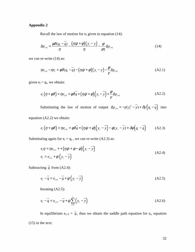
Appendix 2

Recall the law of motion for et given in equation (14):

( ) ( )1 1

( ) ttt t

y yq qe yηψ φφδ φ

η η γη+ +

+ −−∆ = − − ∆ (14)

we can re-write (14) as:

( )( )1 1( )t t t t te e q q y y yφη η φδ ηψ φγ+ +− = − − + − − ∆ (A2.1)

given et = qt, we obtain:

( ) ( )( )1 1t t t te e q y y yφη φδ η φδ ηψ φγ+ ++ = + + + − + ∆ (A2.2)

Substituting the law of motion of output ( )1 ( )dt t ty y y q qγ δγ+∆ = − − + − into

equation (A2.2) we obtain:

( ) ( ) ( ) ( )1 ( )t t t t te e q y y y y q qη φδ η φδ ηψ φ φ δφ++ = + + + − − − + − (A2.3)

Substituting again for et = qt , we can re-write (A2.3) as:

( )( )( )

1

1

t t t

t t t

e e y y

e e y y

η η ηψ φ φ

ψ

+

+

= + + + − −

= + − (A2.4)

Subtracting q from (A2.4):

( )1t t te q e q y yψ+− = − + − (A2.5)

Iterating (A2.5):

( )t t T ts t

e q e q y yψ∞

+=

− = − + −∑ (A2.6)

In equilibrium et+T = q , thus we obtain the saddle path equation for et, equation

(15) in the text:

33

( )t ts t

e q y yψ∞

=

= + −∑ (A2.7)

Alternatively, equation (A2.7) can be derived from equation (13) and (2’):

it = - ψ(yt - y ) = et+1 - et = qt+1 - qt (A2.8)

( )1t t te e y yψ+= + − (A2.9)

Once again, subtracting q and iterating we obtain equation (A2.7):

( )t ts t

e q y yψ∞

=

= + −∑ (A2.7)

34

References

Bank for International Settlements, (2000), Annual Report, Basle June.

Blanchard, O. (1981) “Output, the Stock Market, and Interest Rates” American Economic

Review, Volume 77, Issue 1, 132-143

Corsetti, G. (2000) A perspective on the Euro. Working Paper

Donrbusch, Rudiger (1976) “Expectation and Exchange Rate dynamics” Journal of

Political Economy 84 (December).

Economic Consensus “Consensus Forecasts” various issues.

The Economist “Financial Indicators” various issues.

Financial Times Set 14th, 2000

Greenspan, Alan “Information, productivity and capital investment” Remarks before the

Business Council, Boca Raton, Florida. October 28, 1999.

______________ “Technology and the Economy” Remarks before the Economic Club of

New York. New York. January 13, 2000.

Gordon, Robert J. (1997). “The Time Varying NAIRU and its Implications for Economic

Policy” Journal of Economic Perspectives, Volume II, number 1.

Gordon, Robert J. and Stephen King (1982) “The Output Cost of Disinflation in a

Traditional and Vector Autoregressive Models” Brookings Papers on Economic

Activity, I.

Hoffman D. L., Rasche R.H., Tieslau M.A. (1995) “The stability of the long run money

demand in five industrial countries”. Journal of Monetary Economics, 35.

International Monetary Fund, International Financial Statistics, various issues.

______________, World Economic Outlook, 2000.

35

Krugman.” Reckonings; Play of the Week” September 20, 2000, The New York Times.

Lucas Jr. R. E. (1982) “Interest rates and currency prices in a two-country world.”

Journal of Monetary Economics 10 (November), 3335-60.

______________ (1988) “Money Demand in the United States: a Quantitative Review”

Carnegie-Rochester Conference Series on Public Policy 29, 137-168.

Mankiw, N Gregory (2000); Macroeconomics. Fourth Edition Worth Publishers.

Mankiw, N Gregory; Summers, Lawrence H. (1986) “Money Demand and the Effects of

Fiscal Policies” Journal of Money, Credit & Banking. Vol. 18 (4). p 415-29.

Mussa, Michael (1984) “ The theory of exchange rate determination.” In John F. O bilson

and Richard C. Marston, eds., Exchange rate theory and practice. Chicago

University Press.

Obstfled, Maurice and Kenneth Rogoff (1995). “Exchange Rate Dynamics Redux“ The

Journal of Political Economy, vol 103, Issue 3.

_____________ (1996), Foundations of International Macroeconomics. The MIT Press.

_____________ (2000), “New directions for stochastic open economy models”, Journal

of International Economics, Vol 50, No1, February 2000.

Staiger, D., Stock J.H, Watson M.W., (1996), “ How precise are estimates of the natural

rate of unemployment” NBER Working Paper, 5477.

Stockman, Alan C. (1980) “A theory of Exchange rate determination.” Journal of

Political Economy 88 (August): 673-98.

Stock J.H, Watson M.W., 1983 A simple estimator of cointegrating vectors in higher

order integrated system. Econometrica 61.

U.S. Department of Commerce, U.S. Trade in Goods and Services. Various years.

36

Figure 1

Balance of Goods and Services (as a % of GDP)

-3.5

-3.0

-2.5

-2.0

-1.5

-1.0

1995: I 1996: I 1997: I 1998: I 1999: I 2000: I

1995:I-2000:III

Figure 2

Log* of the Trade Balance Deficit as a % of GDP

-1.4

-1.2

-1.0

-0.8

-0.6

-0.4

-0.2

0.0

1995: I 1996: I 1997: I 1998: I 1999: I 2000: I

1995:I-2000:III*Chart shows minus log of the trade balance deficit

37

Figure 3

Evolution of Output, Real and Nomial Exchange Rate Constant-Money-Supply Case

-0.300

-0.250

-0.200

-0.150

-0.100

-0.050

0.000

0.050

0.100

0.150

1 4 7 10 13 16 19 22 25 28 31 34 37 40 43 46 49 52

Years

ytqtet

Figure 4

Evolution of Output, Real and Nomial Exchange RateConstant-Price Case

-0.300

-0.250

-0.200

-0.150

-0.100

-0.050

0.000

0.050

0.100

0.150

1 4 7 10 13 16 19 22 25 28 31 34 37 40 43 46 49 52

Years

ytet=qt

38

Figure 5

Evolution of the Interest Rate

0.000

0.005

0.010

0.015

0.020

0.025

0.030

1 4 7 10 13 16 19 22 25 28 31 34 37 40 43 46

Years

r constant pr constant m

Figure 6

Evolution of the Price Level Constant-Money-Suply Case

-0.12

-0.10

-0.08

-0.06

-0.04

-0.02

0.00

1 4 7 10 13 16 19 22 25 28 31 34 37 40 43 46

Years

p

39

Figure 7

Evolution of the Money Supply Constant-Price Case

-0.020

0.000

0.020

0.040

0.060

0.080

0.100

0.120

1 4 7 10 13 16 19 22 25 28 31 34 37 40 43 46

Years

m