Chapter 4

TFOCS

Most of this chapter is part of a journal article submission “Templates for Convex Cone Problems

with Applications to Sparse Signal Recover” [BCG10a], and was jointly written with Emmanuel

Candes and Michael Grant. An accompanying software package called “Templates for First-Order

Conic Solvers” (TFOCS) is available for download [BCG10b].

Parts of this chapter are new and do not appear in the journal version. The section §4.6 re-

derives the dual problem in a dual function framework, as opposed to a dual cone framework. The

end algorithm is the same, but the new formulation has the benefit of making certain requirements

very clear. This also allows for certain new convergence results, which are presented in §4.6.4. The

appendix §4.12 has been rewritten and also incorporates work in the literature which very recently

appeared. A section on extensions, §4.8, considers a method for automatically determining the

restart parameter (§4.8.1), and includes discussion (§4.8.2) on the special problems of noiseless basis

pursuit, conic programs in standard form, and matrix completion.

This chapter develops a general framework for solving a variety of convex cone problems that

frequently arise in signal processing, machine learning, statistics, and other fields. The approach

works as follows: first, determine a conic formulation of the problem; second, determine its dual;

third, apply smoothing; and fourth, solve using an optimal first-order method. A merit of this

approach is its flexibility: for example, all compressed sensing problems can be solved via this

approach. These include models with objective functionals such as the total-variation norm, ‖Wx‖1where W is arbitrary, or a combination thereof. In addition, the chapter introduces a number of

technical contributions such as a novel continuation scheme and a novel approach for controlling

the step size, and applies results showing that the smooth and unsmoothed problems are sometimes

formally equivalent. Combined with our framework, these lead to novel, stable, and computationally

efficient algorithms. For instance, our general implementation is competitive with state-of-the-art

methods for solving intensively studied problems such as the LASSO. Further, numerical experiments

show that one can solve the Dantzig selector problem, for which no efficient large-scale solvers exist,

in a few hundred iterations. Finally, the chapter is accompanied with a software release. This

196

software is not a single, monolithic solver; rather, it is a suite of programs and routines designed to

serve as building blocks for constructing complete algorithms.

4.1 Introduction

4.1.1 Motivation

This chapter establishes a general framework for constructing optimal first-order methods for solving

certain types of convex optimization programs that frequently arise in signal and image processing,

statistics, computer vision, and a variety of other fields.1 In particular, we wish to recover an

unknown vector x0 ∈ Rn from the data y ∈ Rm and the model

y = Ax0 + z; (4.1.1)

here, A is a knownm×n design matrix and z is a noise term. To fix ideas, suppose we find ourselves in

the increasingly common situation where there are fewer observations/measurements than unknowns,

i.e., m < n. While this may seem a priori hopeless, an impressive body of recent works has

shown that accurate estimation is often possible under reasonable sparsity constraints on x0. One

practically and theoretically effective estimator is the Dantzig selector introduced in [CT07a]. The

idea of this procedure is rather simple: find the estimate which is consistent with the observed data

and has minimum `1 norm (thus promoting sparsity). Formally, assuming that the columns of A

are normalized,2 the Dantzig selector is the solution to the convex program

minimize ‖x‖1subject to ‖A∗(y −Ax)‖∞ ≤ δ,

(4.1.2)

where δ is a scalar. Clearly, the constraint is a data fitting term since it asks that the correlation

between the residual vector r = y − Ax and the columns of A is small. Typically, the scalar δ is

adjusted so that the true x0 is feasible, at least with high probability, when the noise term z is

stochastic; that is, δ obeys ‖A∗z‖∞ ≤ δ (with high probability). Another effective method, which

we refer to as the LASSO [Tib96] (also known as basis pursuit denoising, or BPDN), assumes a

different fidelity term and is the solution to

minimize ‖x‖1subject to ‖y −Ax‖2 ≤ ε,

(4.1.3)

1The meaning of the word “optimal” shall be made precise later.2There is a slight modification when the columns do not have the same norm, namely, ‖D−1A∗(y − Ax)‖∞ ≤ δ,

where D is diagonal and whose diagonal entries are the `2 norms of the columns of A.

197

where ε is a scalar, which again may be selected so that the true vector is feasible. Both of these

estimators are generally able to accurately estimate nearly sparse vectors and it is, therefore, of

interest to develop effective algorithms for each that can deal with problems involving thousands or

even millions of variables and observations.

There are of course many techniques, which are perhaps more complicated than (4.1.2) and

(4.1.3), for recovering signals or images from possibly undersampled noisy data. Suppose for instance

that we have noisy data y (4.1.1) about an n×n image x0; that is, [x0]ij is an n2-array of real numbers.

Then to recover the image, one might want to solve a problem of this kind:

minimize ‖Wx‖1 + λ‖x‖TV

subject to ‖y −Ax‖2 ≤ ε,(4.1.4)

where W is some (possibly non-orthogonal) transform such as an undecimated wavelet transform

enforcing sparsity of the image in this domain, and ‖ · ‖TV is the isotropic total-variation norm

introduced in [ROF92] defined as

‖x‖TV :=∑i,j

√|x[i+ 1, j]− x[i, j]|2 + |x[i, j + 1]− x[i, j]|2.

The motivation for (4.1.4) is to look for a sparse object in a transformed domain while reducing

artifacts due to sparsity constraints alone, such as Gibbs oscillations, by means of the total-variation

norm [ROF92,CG02,CR05]. The proposal (4.1.4) appears computationally more involved than both

(4.1.2) and (4.1.3), and our goal is to develop effective algorithms for problems of this kind as well.

To continue our tour, another problem that has recently attracted a lot attention concerns the

recovery of a low-rank matrix X0 from undersampled data

y = A(X0) + z, (4.1.5)

where A : Rn1×n2 → Rm is a linear operator supplying information about X0. An important

example concerns the situation where only some of the entries of X0 are revealed, A(X0) = [X0]ij :

(i, j) ∈ E ⊂ [n1] × [n2], and the goal is to predict the values of all the missing entries. It has been

shown [CR09,CT10,Gro11] that an effective way of recovering the missing information from y and

the model (4.1.5) is via the convex program

minimize ‖X‖∗subject to X ∈ C.

(4.1.6)

Here, ‖X‖∗ is the sum of the singular values of the matrix X, a quantity known as the nuclear

norm of X. (‖X‖∗ is also the dual of the standard operator norm ‖X‖, given by the largest singular

198

value of X). Above, C is a data fitting set, and might be {X : A(X) = y} in the noiseless case,

or {X : ‖A∗(y − A(X))‖∞ ≤ δ} (Dantzig selector-type constraint), or {X : ‖y − A(X)‖2 ≤ ε}(LASSO-type constraint) in the noisy setup. We are again interested in computational solutions to

problems of this type.

4.1.2 The literature

There is of course an immense literature for solving problems of the types described above. Consider

the LASSO, for example. Most of the works [HYZ08,WYGZ10,OMDY10,YOGD08,FNW07,WNF09,

BT09,FHT10] are concerned with the unconstrained problem

minimize 12‖Ax− b‖22 + λ‖x‖1, (4.1.7)

which differs from (4.1.3) in that the hard constraint ‖Ax − b‖2 ≤ ε is replaced with a quadratic

penalty 12λ−1‖Ax − b‖22. There are far fewer methods specially adapted to (4.1.3); let us briefly

discuss some of them. SPGL1 [vdBF08] is a solver specifically designed for (4.1.3), and evidence

from [BBC11] suggests that it is both robust and efficient. The issue is that at the moment, it

cannot handle important variations such as

minimize ‖Wx‖1subject to ‖y −Ax‖2 ≤ ε,

where W is an over-complete (i.e., more columns than rows) transform as in (4.1.4). The main

reason is that SPGL1—as with almost all first-order methods for that matter—relies on the fact

that the proximity operator associated with the `1 norm,

x(z; t) , argminx∈Rn

12 t−1‖x− z‖22 + ‖x‖1, (4.1.8)

is efficiently computable via soft-thresholding. This is not the case, however, when ‖x‖1 is replaced

by a general term of the form ‖Wx‖1, except in the special cases when WW ∗ = I [CP07b], and

these special cases cannot occur if W is over-complete. NESTA [BBC11] can efficiently deal with an

objective functional of the form ‖Wx‖1—that is, it works for any W and the extra computational

cost is just one application of W and W ∗ per iteration—but it requires repeated projections onto

the feasible set; see also [ABDF11] for a related approach, and [WBFA09] for a similar approach

specialized for minimizing total variation. Hence, NESTA is efficient when AA∗ is a projector or,

more generally, when the eigenvalues of AA∗ are well clustered. Other types of algorithms such as

LARS [EHJT04] are based on homotopy methods, and compute the whole solution path; i.e., they

find the solution to (4.1.7) for all values of the regularization parameter λ and, in doing so, find the

199

solution to the constrained problem (4.1.3). These methods do not scale well with problem size,

however, especially when the solution is not that sparse.

The approach taken in this chapter, described in §4.1.3, is based off duality and smoothing, and

these concepts have been widely studied in the literature. At the heart of the method is the fact

that solving the dual problem eliminates difficulties with affine operators A, and this observation

goes back to Uzawa’s method [Cia89]. More recently, [MZ09, CP10c, CDV10] discuss dual method

approaches to signal processing problems. In [MZ09], a non-negative version of (4.1.3) (which can

be extended to the regular version by splitting x into positive and negative parts) is solved using

inner and outer iterations. The outer iteration allows the inner problem to be smoothed, which

is similar to the continuation idea presented in §4.5.5. The outer iteration is proved to converge

rapidly, but depends on exactly solving the inner iteration. The work in [LST11] applies a similar

outer iteration, which they recognize as the proximal point algorithm, applied to nuclear norm

minimization. The method of [CP10c] applies a primal-dual method to unconstrained problems

such as (4.1.7), or simplified and unconstrained versions of (4.1.4). Notably, they prove that when

the objective function contains an appropriate strongly convex term, then the primal variable xk

converges with the bound ‖xk − x?‖22 ≤ O(1/k2). The approach of [CDV10] considers smoothing

(4.1.3) in a similar manner to that discussed in §4.2.4, but does not use continuation to diminish

the effect of the smoothing. The dual problem is solved via the forward-backward method, and this

allows the authors to prove that the primal variable converges, though without a known bound on

the rate.

Turning to the Dantzig selector, solution algorithms are scarce. The standard way of solving

(4.1.2) is via linear programming techniques [CR07b] since it is well known that it can be recast as

a linear program [CT07a]. Typical modern solvers rely on interior-point methods (IPM) which are

somewhat problematic for large-scale problems, since they do not scale well with size. Another way

of solving (4.1.2) is via the new works [JRL09, Rom08], which use homotopy methods inspired by

LARS to compute the whole solution path of the Dantzig selector. These methods, however, are also

unable to cope with large problems. As an example of the speed of these methods, the authors of

l1ls [KKB07], which is a log-barrier interior-point method using preconditioned conjugate-gradients

to solve the Newton step, report that on an instance of the (4.1.7) problem, their method is 20×faster than the commercial IPM MOSEK [Mos02], 10× faster than the IPM PDCO [SK02], 78×faster than IPM l1Magic [CR07b], and 1.6× faster than Homotopy [DT08]. Yet the first-order

method FPC [HYZ08] reports that FPC is typically 10 to 20× faster than l1ls, and sometimes even

1040× faster. These results are for (4.1.7) and not the Dantzig selector, but it is reasonable to

conclude that in general IPM and homotopy do not seem reasonable methods for extremely large

problems.

The accelerated first-order algorithm recently introduced in [Lu09] can handle large Dantzig

200

selector problems, but with the same limitations as NESTA since it requires inverting AA∗. A

method based on operator splitting has been suggested in [FS09] but results have not yet been

reported. Another alternative is adapting SPGL1 to this setting, but this comes with the caveat

that it does not handle slight variations as discussed above.

Finally, as far as the mixed norm problem (4.1.4) is concerned, we are not aware of efficient

solution algorithms. One can always recast this problem as a second-order cone program (SOCP)

which one could then solve via an interior-point method; but again, this is problematic for large-scale

problems.

4.1.3 Our approach

In this chapter, we develop a template for solving a variety of problems such as those encountered

thus far. The template proceeds as follows: first, determine an equivalent conic formulation; second,

determine its dual; third, apply smoothing; and fourth, solve using an optimal first-order method.

4.1.3.1 Conic formulation

In reality, our approach can be applied to general models expressed in the following canonical form:

minimize f(x)

subject to A(x) + b ∈ K.(4.1.9)

The optimization variable is a vector x ∈ Rn, and the objective function f is convex, possibly

extended-valued, and not necessarily smooth. The constraint is expressed in terms of a linear

operator A : Rn → Rm, a vector b ∈ Rm, and a closed, convex cone K ⊆ Rm. We shall call a model

of the form (4.1.9) that is equivalent to a given convex optimization model P a conic form for P.

The conic constraint A(x) + b ∈ K may seem specialized, but in fact any closed convex subset of

Rn may be represented in this fashion; and models involving complex variables, matrices, or other

vector spaces can be handled by defining appropriate isomorphisms. Of course, some constraints

are more readily transformed into conic form than others; included in this former group are linear

equations, linear inequalities, and convex inequalities involving norms of affine forms. Thus virtually

every convex compressed sensing model may be readily converted. Almost all models admit multiple

conic forms, and each results in a different final algorithm.

For example, the Dantzig selector (4.1.2) can be mapped to conic form as follows:

f(x)→ ‖x‖1, A(x)→ (A∗Ax, 0), b→ (−A∗y, δ), K → Ln∞, (4.1.10)

where Ln∞ is the epigraph of the `∞ norm: Ln∞ = {(y, t) ∈ Rn+1 : ‖y‖∞ ≤ t}.

201

4.1.3.2 Dualization

The conic form (4.1.9) does not immediately lend itself to efficient solution using first-order methods

for two reasons: first, because f may not be smooth; and second, because projection onto the set

{x | A(x)+b ∈ K}, or even the determination of a single feasible point, can be expensive. We propose

to resolve these issues by solving either the dual problem, or a carefully chosen approximation of it.

Recall that the dual of our canonical form (4.1.9) is given by

maximize g(λ)

subject to λ ∈ K∗,(4.1.11)

where g(λ) is the Lagrange dual function

g(λ) , infxL(x, λ) = inf

xf(x)− 〈λ,A(x) + b〉,

and K∗ is the dual cone defined via

K∗ = {λ ∈ Rm : 〈λ, x〉 ≥ 0 for all x ∈ K}.

The dual form has an immediate benefit that for the problems of interest, projections onto

the dual cone are usually tractable and computationally very efficient. For example, consider the

projection of a point onto the feasible set {x : ‖Ax − y‖2 ≤ ε} of the LASSO, an operation which

may be expensive. However, one can recast the constraint as A(x) + b ∈ K with

A(x)→ (Ax, 0), b→ (−y, ε) K → Lm2 , (4.1.12)

where Lm2 is the second-order cone Lm2 = {(y, t) ∈ Rm+1 : ‖y‖2 ≤ t}. This cone is self dual, i.e.,

(Lm2 )∗ = Lm2 , and projection onto Lm2 is trivial: indeed, it is given by

(y, t) 7→

(y, t), ‖y‖2 ≤ t,

c(y, ‖y‖2), −‖y‖2 ≤ t ≤ ‖y‖2,

(0, 0), t ≤ −‖y‖2,

c =‖y‖2 + t

2‖y‖2. (4.1.13)

And so we see that by eliminating the affine mapping, the projection computation has been greatly

simplified. Of course, not every cone projection admits as simple a solution as (4.1.13); but as we

will show, all of the cones of interest to us do indeed.

202

4.1.3.3 Smoothing

Unfortunately, because of the nature of the problems under study, the dual function is usually not

differentiable either, and direct solution via subgradient methods would converge too slowly. Our

solution is inspired by the smoothing technique due to Nesterov [Nes05]. We shall see that if one

modifies the primal objective f(x) and instead solves

minimize fµ(x) , f(x) + µd(x)

subject to A(x) + b ∈ K,(4.1.14)

where d(x) is a strongly convex function to be defined later and µ a positive scalar, then the dual

problem takes the form

maximize gµ(λ)

subject to λ ∈ K∗,(4.1.15)

where gµ is a smooth approximation of g. This approximate model can now be solved using first-

order methods. As a general rule, higher values of µ improve the performance of the underlying

solver, but at the expense of accuracy. Techniques such as continuation can be used to recover the

accuracy lost, however, so the precise trade-off is not so simple.

In many cases, the smoothed dual can be reduced to an unconstrained problem of the form

maximize −gsmooth(z)− h(z), (4.1.16)

with optimization variable z ∈ Rm, where gsmooth is convex and smooth and h convex, non-smooth,

and possibly extended-valued. For instance, for the Dantzig selector (4.1.2), h(z) = δ‖z‖1. As

we shall see, this so-called composite form can also be solved efficiently using optimal first-order

methods. In fact, the reduction to composite form often simplifies some of the central computations

in the algorithms.

4.1.3.4 First-order methods

Optimal first-order methods are proper descendants of the classic projected gradient algorithm. For

the smoothed dual problem (4.1.15), a prototypical projected gradient algorithm begins with a point

λ0 ∈ K∗, and generates updates for k = 0, 1, 2, ... as follows:

λk+1 ← argminλ∈K∗

‖λk + tk∇gµ(λk)− λ‖2, (4.1.17)

203

given step sizes {tk}. The method has also been extended to composite problems like (4.1.16)

[Wri07,Nes07,Tse08]; the corresponding iteration is

zk+1 ← argminy

gsmooth(zk) + 〈∇gsmooth(zk), z − zk〉+ 12tk‖z − zk‖2 + h(z). (4.1.18)

Note the use of a general norm ‖ · ‖ and the inclusion of the non-smooth term h. We call the

minimization in (4.1.18) a generalized projection, because it reduces to a standard projection (4.1.17)

if the norm is Euclidean and h is an indicator function. This generalized form allows us to construct

efficient algorithms for a wider variety of models.

For the problems under study, the step sizes {tk} above can be chosen so that ε-optimality (that

is, supλ∈K∗ gµ(λ) − gµ(λk) ≤ ε) can be achieved in O(1/ε) iterations [Nes04]. In 1983, Nesterov

reduced this cost to O(1/√ε) using a slightly more complex iteration

λk+1 ← argminλ∈K∗

‖νk + tk∇gµ(νk)− λ‖2, νk+1 ← λk+1 + αk(λk+1 − λk), (4.1.19)

where ν0 = λ0 and the sequence {αk} is constructed according to a particular recurrence relation.

Previous work by Nemirosvski and Yudin had established O(1/√ε) complexity as the best that can

be achieved for this class of problems [NY83], so Nesterov’s modification is indeed optimal. Many

alternative first-order methods have since been developed [Nes88,Nes05,Nes07,Tse08,AT06,LLM09],

including methods that support generalized projections. We examine these methods in more detail

in §4.5.

We have not yet spoken about the complexity of computing gµ or gsmooth and their gradients.

For now, let us highlight the fact that ∇gµ(λ) = −A(x(λ))− b, where

x(λ) , argminxLµ(x, λ) = argmin

xf(x) + µd(x)− 〈A(x) + b, λ〉, (4.1.20)

and d(x) is a selected proximity function. In the common case that d(x) = 12‖x−x0‖2, the structure

of (4.1.20) is identical to that of a generalized projection. Thus we see that the ability to efficiently

minimize the sum of a linear term, a proximity function, and a non-smooth function of interest is

the fundamental computational primitive involved in our method. Equation (4.1.20) also reveals

how to recover an approximate primal solution as λ approaches its optimal value.

4.1.4 Contributions

The formulation of compressed sensing models in conic form is not widely known. Yet the convex op-

timization modeling framework CVX [GB10] converts all models into conic form; and the compressed

sensing package `1-Magic [CR07b] converts problems into second-order cone programs (SOCPs).

Both systems utilize interior-point methods instead of first-order methods, however. As mentioned

204

above, the smoothing step is inspired by [Nes05], and is similar in structure to traditional Lagrangian

augmentation. As we also noted, first-order methods have been a subject of considerable research.

Taken separately, then, none of the components in this approach is new. However their combi-

nation and application to solve compressed sensing problems leads to effective algorithms that have

not previously been considered. For instance, applying our methodology to the Dantzig selector

gives a novel and efficient algorithm (in fact, it gives several novel algorithms, depending on which

conic form is used). Numerical experiments presented later in the chapter show that one can solve

the Dantzig selector problem with a reasonable number of applications of A and its adjoint; the

exact number depends upon the desired level of accuracy. In the case of the LASSO, our approach

leads to novel algorithms which are competitive with state-of-the-art methods such as SPGL1.

Aside from good empirical performance, we believe that the primary merit of our framework lies

in its flexibility. To be sure, all the compressed sensing problems listed at the beginning of this

chapter, and of course many others, can be solved via this approach. These include total-variation

norm problems, `1-analysis problems involving objectives of the form ‖Wx‖1 where W is neither

orthogonal nor diagonal, and so on. In each case, our framework allows us to construct an effective

algorithm, thus providing a computational solution to almost every problem arising in sparse signal

or low-rank matrix recovery applications.

Furthermore, in the course of our investigation, we have developed a number of additional tech-

nical contributions. For example, we will show that certain models, including the Dantzig selector,

exhibit an exact penalty property: the exact solution to the original problem is recovered even when

some smoothing is applied. We have also developed a novel continuation scheme that allows us to

employ more aggressive smoothing to improve solver performance while still recovering the exact

solution to the unsmoothed problem. The flexibility of our template also provides opportunities to

employ novel approaches for controlling the step size.

4.1.5 Software

This chapter is accompanied with a software release [BCG10b], including a detailed user guide which

gives many additional implementation details not discussed in this chapter. Since most compressed

sensing problems can be easily cast into standard conic form, our software provides a powerful and

flexible computational tool for solving a large range of problems researchers might be interested in

experimenting with.

The software is not a single, monolithic solver; rather, it is a suite of programs and routines

designed to serve as building blocks for constructing complete algorithms. Roughly speaking, we

can divide the routines into three levels. On the first level is a suite of routines that implement a

variety of known first-order solvers, including the standard projected gradient algorithm and known

optimal variants by Nesterov and others. On the second level are wrappers designed to accept

205

problems in conic standard form (4.1.9) and apply the first-order solvers to the smoothed dual

problem. Finally, the package includes a variety of routines to directly solve the specific models

described in this chapter and to reproduce our experiments.

We have worked to ensure that each of the solvers is as easy to use as possible, by providing

sensible defaults for line search, continuation, and other factors. At the same time, we have sought

to give the user flexibility to insert their own choices for these components. We also want to provide

the user with the opportunity to compare the performance of various first-order variants on their

particular application. We do have some general views about which algorithms perform best for

compressed sensing applications, however, and will share some of them in §4.7.

4.1.6 Organization of the chapter

In §4.2, we continue the discussion of conic formulations, including a derivation of the dual conic for-

mulation and details about the smoothing operation. Section 4.3 instantiates this general framework

to derive a new algorithm for the Dantzig selector problem. In §4.4, we provide further selected in-

stantiations of our framework including the LASSO, total-variation problems, `1-analysis problems,

and common nuclear-norm minimization problems. In §4.5, we review a variety of first-order meth-

ods and suggest improvements. Section 4.6 derives the dual formulation using the machinery of

dual functions instead of dual cones, and covers known convergence results. Section 4.7 presents

numerical results illustrating both the empirical effectiveness and the flexibility of our approach.

Some interesting special cases are discussed in 4.8, such as solving linear program in standard form.

Section 4.9 provides a short introduction to the software release accompanying this chapter. Finally,

the appendix gives a proof of the exact penalty property for general linear programs (which itself is

not a novel result), and thus for Dantzig selector and basis pursuit models, and describes a unique

approach we use to generate test models so that their exact solution is known in advance.

4.2 Conic formulations

4.2.1 Alternate forms

In the introduction, we presented our standard conic form (4.1.9) and a specific instance for the

Dantzig selector in (4.1.10). As we said then, conic forms are rarely unique; this is true even if one

disregards simple scalings of the cone constraint. For instance, we may express the Dantzig selector

constraint as an intersection of linear inequalities, −δ1 � A∗(y−Ax) � δ1, suggesting the following

alternative:

f(x)→ ‖x‖1, A(x)→

−A∗AA∗A

x, b→

δ1 +A∗y

δ1−A∗y

, K → R2n+ . (4.2.1)

206

We will return to this alternative later in §4.3.5. In many instances, a conic form may involve the

manipulation of the objective function as well. For instance, if we first transform (4.1.2) to

minimize t

subject to ‖x‖1 ≤ t‖A∗(y −Ax)‖∞ ≤ δ,

then yet another conic form results:

f(x, t)→ t, A(x, t)→ (x, t, A∗Ax, 0), b→ (0, 0,−A∗y, δ), K → Ln1 × Ln∞, (4.2.2)

where Ln1 is the epigraph of the `1 norm, Ln1 = {(y, t) ∈ Rn+1 : ‖y‖1 ≤ t}.Our experiments show that different conic formulations yield different levels of performance using

the same numerical algorithms. Some are simpler to implement than others as well. Therefore, it is

worthwhile to at least explore these alternatives to find the best choice for a given application.

4.2.2 The dual

To begin with, the conic Lagrangian associated with (4.1.9) is given by

L(x, λ) = f(x)− 〈λ,A(x) + b〉, (4.2.3)

where λ ∈ Rm is the Lagrange multiplier, constrained to lie in the dual cone K∗. The dual function

g : Rm → (R ∪ {−∞}) is, therefore,

g(λ) = infxL(x, λ) = −f∗(A∗(λ))− 〈b, λ〉. (4.2.4)

Here, A∗ : Rm → Rn is the adjoint of the linear operator A and f∗ : Rn → (R∪{+∞}) is the convex

conjugate of f defined by

f∗(z) = supx〈z, x〉 − f(x).

Thus the dual problem is given by

maximize −f∗(A∗(λ))− 〈b, λ〉subject to λ ∈ K∗.

(4.2.5)

Given a feasible primal/dual pair (x, λ), the duality gap is the difference between their respective

objective values. The non-negativity of the duality gap is easily verified:

f(x)− g(λ) = f(x) + f∗(A∗(λ)) + 〈b, λ〉 ≥ 〈x,A∗(λ)〉+ 〈b, λ〉 = 〈A(x) + b, λ〉 ≥ 0. (4.2.6)

207

The first inequality follows from the definition of conjugate functions, while the second follows from

the definition of the dual cone. If both the primal and dual are strictly feasible—as is the case for all

problems we are interested in here—then the minimum duality gap is exactly zero, and there exists

an optimal pair (x?, λ?) that achieves f(x?) = g(λ?) = L(x?, λ?). It is important to note that the

optimal points are not necessarily unique; more about this in §4.2.4. But any optimal primal/dual

pair will satisfy the KKT optimality conditions [BV04]

A(x?) + b ∈ K, λ? ∈ K∗, 〈A(x?) + b, λ?〉 = 0, A∗(λ?) ∈ ∂f(x?), (4.2.7)

where ∂f refers to the subgradient of f .

4.2.3 The differentiable case

The dual function is of course concave; and its derivative (when it exists) is given by

∇g(λ) = −A(x(λ))− b, x(λ) ∈ argminxL(x, λ). (4.2.8)

It is possible that the minimizer x(λ) is not unique, so in order to be differentiable, all such minimizers

must yield the same value of −A(x(λ))− b [BNO03].

If g is finite and differentiable on the entirety of K∗, then it becomes trivial to locate an initial

dual point (e.g., λ = 0); and for many genuinely useful cones K∗, it becomes trivial to project an

arbitrary point λ ∈ Rm onto this feasible set. If the argmin calculation in (4.2.8) is computationally

practical, we may entertain the construction of a projected gradient method for solving the dual

problem (4.2.5) directly; i.e., without our proposed smoothing step. Once an optimal dual point

λ? is recovered, an optimal solution to the original problem (4.1.9) is recovered by solving x? ∈argminx L(x, λ?) ∩ {x : Ax + b ∈ K}. If argminx L(x, λ?) is unique, which is the case when f is

strictly convex, then this minimizer is necessarily feasible and is the primal optimal solution.

Further suppose that f is strongly convex3 ; that is, it satisfies for some constant mf > 0,

f((1− α)x+ αx′) ≤ (1− α)f(x) + αf(x′)−mfα(1− α)‖x− x′‖22/2 (4.2.9)

for all x, x′ ∈ dom(f) = {x : f(x) < +∞} and 0 ≤ α ≤ 1. Then assuming the problem is feasible,

it admits a unique optimal solution. The Lagrangian minimizers x(λ) are unique for all λ ∈ Rn;

so g is differentiable everywhere. Furthermore, [Nes05] proves that the gradient of g is Lipschitz

continuous, obeying

‖∇g(λ′)−∇g(λ)‖2 ≤ m−1f ‖A‖2‖λ′ − λ‖2, (4.2.10)

3 We use the Euclidean norm, but any norm works as long as ‖A‖ in (4.2.10) is appropriately defined; see [Nes05].

208

where ‖A‖ = sup‖x‖2=1 ‖A(x)‖2 is the induced operator norm of A. So when f is strongly convex,

then provably convergent, accelerated gradient methods in the Nesterov style are possible.

4.2.4 Smoothing

Unfortunately, it is more likely that g is not differentiable (or even finite) on all of K∗. So we consider

a smoothing approach similar to that proposed in [Nes05] to solve an approximation of our problem.

Consider the following perturbation of (4.1.9):

minimize fµ(x) , f(x) + µd(x)

subject to A(x) + b ∈ K(4.2.11)

for some fixed smoothing parameter µ > 0 and a strongly convex function d obeying

d(x) ≥ d(x0) + 12‖x− x0‖2 (4.2.12)

for some fixed point x0 ∈ Rn. Such a function is usually called a proximity function.

The new objective fµ is strongly convex with mf = µ, so the full benefits described in §4.2.3

now apply. The Lagrangian and dual functions become4

Lµ(x, λ) = f(x) + µd(x)− 〈λ,A(x) + b〉 (4.2.13)

gµ(λ) , infxLµ(x, λ) = −(f + µd)∗(A∗(λ))− 〈b, λ〉. (4.2.14)

One can verify that for the affine objective case f(x) , 〈c0, x〉 + d0, the dual and smoothed dual

function take the form

g(λ) = d0 − I`∞(A∗(λ)− c0)− 〈b, λ〉,

gµ(λ) = d0 − µd∗(µ−1(A∗(λ)− c0))− 〈b, λ〉,

where I`∞ is the indicator function of the `∞ norm ball; that is,

I`∞(y) ,

0, ‖y‖∞ ≤ 1,

+∞, ‖y‖∞ > 1.

The new optimality conditions are

A(xµ) + b ∈ K, λµ ∈ K∗, 〈A(xµ) + b, λµ〉 = 0, A∗(λµ)− µ∇d(xµ) ∈ ∂f(xµ). (4.2.15)

4One can also observe the identity gµ(λ) = supz −f∗(A∗(λ)− z)− µd∗(µ−1z)− 〈b, λ〉.

209

Because the Lipschitz bound (4.2.10) holds, first-order methods may be employed to solve (4.2.11)

with provable performance. The iteration counts for these methods are proportional to the square

root of the Lipschitz constant, and therefore proportional to µ−1/2. There is a trade off between the

accuracy of the approximation and the performance of the algorithms that must be explored.5

For each µ > 0, the smoothed model obtains a single minimizer xµ; and the trajectory traced

by xµ as µ varies converges to an optimal solution x? , limµ→0+xµ. Henceforth, when speaking

about the (possibly non-unique) optimal solution x? to the original model, we will be referring to

this uniquely determined value. Later we will show that for some models, including the Dantzig

selector, the approximate model is exact : that is, xµ = x? for sufficiently small but nonzero µ.

Roughly speaking, the smooth dual function gµ is what we would obtain if the Nesterov smoothing

method described in [Nes05] were applied to the dual function g. It is worthwhile to explore how

things would differ if the Nesterov approach were applied directly to the primal objective f(x).

Suppose that f(x) = ‖x‖1 and d(x) = 12‖x‖22. The Nesterov approach yields a smooth approximation

fNµ whose elements can be described by the formula

[fNµ (x)

]i

= sup|z|≤1

zxi − 12µz

2 =

12µ−1x2

i , |xi| ≤ µ,

|xi| − 12µ, |x| ≥ µ,

i = 1, 2, . . . , n. (4.2.16)

Readers may recognize this as the Huber penalty function with half-width µ; a graphical comparison

with fµ is provided in Figure 4.1. Its smoothness may seem to be an advantage over our choice

fµ(x) = ‖x‖1 + 12‖x‖22, but the difficulty of projecting onto the set {x | A(x) + b ∈ K} remains; so

we still prefer to solve the dual problem. Furthermore, the quadratic behavior of fNµ around xi = 0

eliminates the tendency towards solutions with many zero values. In contrast, fµ(x) maintains the

sharp vertices from the `1 norm that are known to encourage sparse solutions.

4.2.5 Composite forms

In most of the cases under study, the dual variable can be partitioned as λ , (z, τ) ∈ Rm−m × Rm

such that the smoothed dual gµ(z, τ) is linear in τ ; that is,

gµ(λ) = −gsmooth(z)− 〈vµ, τ〉 (4.2.17)

for some smooth convex function gsmooth and a constant vector vµ ∈ Rm. An examination of

the Lagrangian Lµ (4.2.13) reveals a precise condition under which this occurs: when the linear

operator A is of the form A(x) → (A(x),0m×1), as seen in the conic constraints for the Dantzig

selector (4.1.10) and LASSO (4.1.12). If we partition b = (b, bτ ) accordingly, then evidently vµ = bτ .

5In fact, even when the original objective is strongly convex, further adding a strongly convex term may beworthwhile to improve performance.

210

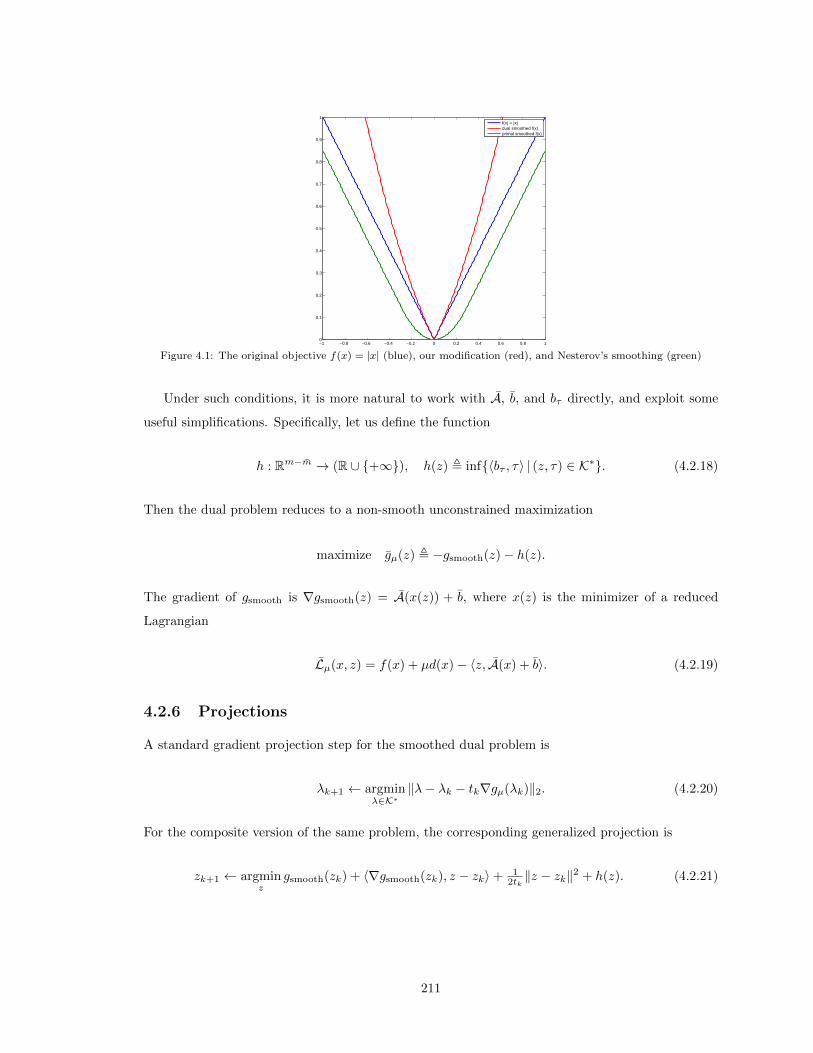
−1 −0.8 −0.6 −0.4 −0.2 0 0.2 0.4 0.6 0.8 10

0.1

0.2

0.3

0.4

0.5

0.6

0.7

0.8

0.9

1

f(x) = |x|dual smoothed f(x)primal smoothed f(x)

Figure 4.1: The original objective f(x) = |x| (blue), our modification (red), and Nesterov’s smoothing (green)

Under such conditions, it is more natural to work with A, b, and bτ directly, and exploit some

useful simplifications. Specifically, let us define the function

h : Rm−m → (R ∪ {+∞}), h(z) , inf{〈bτ , τ〉 | (z, τ) ∈ K∗}. (4.2.18)

Then the dual problem reduces to a non-smooth unconstrained maximization

maximize gµ(z) , −gsmooth(z)− h(z).

The gradient of gsmooth is ∇gsmooth(z) = A(x(z)) + b, where x(z) is the minimizer of a reduced

Lagrangian

Lµ(x, z) = f(x) + µd(x)− 〈z, A(x) + b〉. (4.2.19)

4.2.6 Projections

A standard gradient projection step for the smoothed dual problem is

λk+1 ← argminλ∈K∗

‖λ− λk − tk∇gµ(λk)‖2. (4.2.20)

For the composite version of the same problem, the corresponding generalized projection is

zk+1 ← argminz

gsmooth(zk) + 〈∇gsmooth(zk), z − zk〉+ 12tk‖z − zk‖2 + h(z). (4.2.21)

211

Integrating the definition of∇gsmooth(z) into (4.2.21) and simplifying yields a two-sequence recursion:

xk ← argminx

f(x) + µd(x)− 〈A∗(zk), x〉

zk+1 ← argminz

h(z) + 12tk‖z − zk‖2 + 〈A(xk) + b, z〉.

(4.2.22)

Note the similarity in computational structure of the two formulae. This similarity is even more

evident in the common scenario where d(x) = 12‖x− x0‖2 for some fixed x0 ∈ Rn.

Let Σ be the matrix composed of the first m − m rows of the m ×m identity matrix, so that

Σλ ≡ z for all λ = (z, τ). Then (4.2.21) can also be written in terms of K∗ and gµ:

zk+1 ← Σ · argmaxλ∈K∗

gµ(λk) + 〈∇gµ(λk), λ− λk〉 − 12tk‖Σ(λ− λk)‖2, (4.2.23)

where λk , (zk, h(zk)). If m = 0 and the norm is Euclidean, then Σ = I and the standard projection

(4.2.20) is recovered. So (4.2.21) is indeed a true generalization, as claimed in §4.1.3.4.

The key feature of the composite approach, then, is the removal of the linear variables τ from

the proximity term. Given that they are linearly involved to begin with, this yields a more accurate

approximation of the dual function, so we might expect a composite approach to yield improved

performance. In fact, the theoretical predictions of the number of iterations required to achieve a

certain level of accuracy are identical; and in our experience, any differences in practice seem minimal

at best. The true advantage to the composite approach is that generalized projections more readily

admit analytic solutions and are less expensive to compute.

4.3 A novel algorithm for the Dantzig selector

We now weave together the ideas of the last two sections to develop a novel algorithm for the Dantzig

selector problem (4.1.2).

4.3.1 The conic form

We use the standard conic formulation (4.1.9) with the mapping (4.1.10) as discussed in the intro-

duction, which results in the model

minimize ‖x‖1subject to (A∗(y −Ax), δ) ∈ Ln∞,

(4.3.1)

212

where Lm∞ is the epigraph of the `∞ norm. The dual variable λ, therefore, will lie in the dual cone

(Ln∞)∗ = Ln1 , the epigraph of the `1 norm. Defining λ = (z, τ), the conic dual (4.2.5) is

maximize −I`∞(−A∗Az)− 〈A∗y, z〉 − δτsubject to (z, τ) ∈ Ln1 ,

(4.3.2)

where f∗ = I`∞ is the indicator function of the `∞ norm ball as before. Clearly the optimal value

of τ must satisfy ‖z‖1 = τ ,6 so eliminating it yields

maximize −I`∞(−A∗Az)− 〈A∗y, z〉 − δ‖z‖1. (4.3.3)

Neither (4.3.2) nor (4.3.3) has a smooth objective, so the smoothing approach discussed in §4.2.4

will indeed be necessary.

4.3.2 Smooth approximation

We augment the objective with a strongly convex term

minimize ‖x‖1 + µd(x)

subject to (A∗(y −Ax), δ) ∈ K , Ln∞.(4.3.4)

The Lagrangian of this new model is

Lµ(x; z, τ) = ‖x‖1 + µd(x)− 〈z,A∗(y −Ax)〉 − δτ.

Letting x(z) be the unique minimizer of Lµ(x; z, τ), the dual function becomes

gµ(z, τ) = ‖x(z)‖1 + µd(x(z))− 〈z,A∗(y −Ax(z))〉 − τδ.

Eliminating τ per §4.2.5 yields a composite form gµ(z) = −gsmooth(z)− h(z) with

gsmooth(z) = −‖x(z)‖1 − µd(x(z)) + 〈z,A∗(y −Ax(z))〉, h(z) = δ‖z‖1.

The gradient of gsmooth is ∇gsmooth(z) = A∗(y −Ax(z)).

The precise forms of x(z) and ∇gsmooth depend of course on our choice of proximity function

d(x). For our problem, the simple convex quadratic

d(x) = 12‖x− x0‖22,

6We assume δ > 0 here; if δ = 0, the form is slightly different.

213

for a fixed center point x0 ∈ Rn, works well, and guarantees that the gradient is Lipschitz continuous

with a constant at most µ−1‖A∗A‖2. With this choice, x(z) can be expressed in terms of the soft-

thresholding operation which is a common fixture in algorithms for sparse recovery. For scalars x

and s ≥ 0, define

SoftThreshold(x, s) = sgn(x) ·max{|x| − s, 0} =

x+ s, x ≤ −s,

0, |x| ≤ s,

x− s, x ≥ s.

When the first input x is a vector, the soft-thresholding operation is to be applied componentwise.

Armed with this definition, the formula for x(z) becomes

x(z) = SoftThreshold(x0 − µ−1A∗Az, µ−1).

If we substitute x(z) into the formula for gsmooth(z) and simplify carefully, we find that

gsmooth(z) = − 12µ−1‖ SoftThreshold(µx0 −A∗Az, 1)‖22 + 〈A∗y, z〉+ c,

where c is a term that depends only on constants µ and x0. In other words, to within an additive

constant, gsmooth(z) is a smooth approximation of the non-smooth term I`∞(−A∗Az)+〈A∗y, z〉 from

(4.3.2), and indeed it converges to that function as µ→ 0.

For the dual update, the generalized projection is

zk+1 ← argminz

gsmooth(zk) + 〈∇gsmooth(zk), z − zk〉+ 12tk‖z − zk‖22 + δ‖z‖1. (4.3.5)

A solution to this minimization can also be expressed in terms of the soft thresholding operation:

zk+1 ← SoftThreshold(zk − tkA∗(y −Ax(zk)), tkδ).

4.3.3 Implementation

To solve the model presented in §4.3.2, we considered first-order projected gradient solvers. After

some experimentation, we concluded that the Auslender and Teboulle first-order variant [AT06,

Tse08] is a good choice for this model. We discuss this and other variants in more detail in §4.5, so

for now we will simply present the basic algorithm in Listing 1 below. Note that the dual update

used differs slightly from (4.3.5) above: the gradient ∇gsmooth is evaluated at yk, not zk, and the step

size in the generalized projection is multiplied by θ−1k . Each iteration requires two applications of

both A and A∗, and is computationally inexpensive when a fast matrix-vector multiply is available.

214

Listing 1 Algorithm for the smoothed Dantzig selector

Require: z0, x0 ∈ Rn, µ > 0, step sizes {tk}1: θ0 ← 1, v0 ← z0

2: for k = 0, 1, 2, . . . do

3: yk ← (1− θk)vk + θkzk

4: xk ← SoftThreshold(x0 − µ−1A∗Ayk, µ−1).

5: zk+1 ← SoftThreshold(zk − θ−1k tkA

∗(y −Axk), θ−1k tkδ)

6: vk+1 ← (1− θk)vk + θkzk+1

7: θk+1 ← 2/(1 + (1 + 4/θ2k)1/2)

It is known that for a fixed step size tk , t ≤ µ/‖A∗A‖22, the above algorithm converges in the

sense that gµ(z∗)−gµ(zk) = O(k−2). Performance can be improved through the use of a backtracking

line search for zk, as discussed in §4.5.3 (see also [BT09]). Further, fairly standard arguments in

convex analysis show that the sequence {xk} converges to the unique solution to (4.3.4).

4.3.4 Exact penalty

Theorem 3.1 in [CCS10] can be adapted to show that as µ→ 0, the solution to (4.3.4) converges to

a solution to (4.1.2). But an interesting feature of the Dantzig selector model in particular is that if

µ < µ0 for µ0 sufficiently small, the solutions to the Dantzig selector and to its perturbed variation

(4.3.4) coincide; that is, x? = x?µ. In fact, this phenomenon holds for any linear program (LP).

Theorem 4.3.1 (Exact penalty). Consider an arbitrary LP with objective 〈c, x〉 and having an

optimal solution (i.e., the optimal value is not −∞) and let Q be a positive semidefinite matrix.

Then there is a µ0 > 0 such that if 0 < µ ≤ µ0, any solution to the perturbed problem with objective

〈c, x〉 + 12µ〈x − x0, Q(x − x0)〉 is a solution to LP. Among all the solutions to LP, the solutions to

the perturbed problem are those minimizing the quadratic penalty. In particular, in the (usual) case

where the LP solution is unique, the solution to the perturbed problem is unique and they coincide.

The theorem is not difficult to prove, and first appeared in 1979 due to Mangasarian [MM79].

The special case of noiseless basis pursuit was recently analyzed in [Yin10] using different techniques.

More general results, allowing a range of penalty functions, were proved in [FT07]. Our theorem is a

special case of [FT07] and the earlier results, but we present the proof in Appendix 4.11 since it uses

a different technique than [FT07], is directly applicable to our method in this form, and provides

useful intuition. The result, when combined with our continuation techniques in §4.5.5, is also a new

look at known results about the finite termination of the proximal point algorithm when applied to

linear programs [PT74,Ber75].

As a consequence of the theorem, the Dantzig selector and noiseless basis pursuit, which are

215

10−2

10−1

100

10−10

10−9

10−8

10−7

10−6

10−5

10−4

10−3

10−2

10−1

100

µ

Err

or

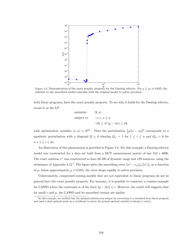
Figure 4.2: Demonstration of the exact penalty property for the Dantzig selector. For µ ≤ µ0 ≈ 0.025, thesolution to the smoothed model coincides with the original model to solver precision.

both linear programs, have the exact penalty property. To see why it holds for the Dantzig selector,

recast it as the LP

minimize 〈1, u〉subject to −u ≤ x ≤ u

−δ1 ≤ A∗(y −Ax) ≤ δ1,

with optimization variables (x, u) ∈ R2n. Then the perturbation 12µ‖x − x0‖2 corresponds to a

quadratic perturbation with a diagonal Q � 0 obeying Qii = 1 for 1 ≤ i ≤ n and Qii = 0 for

n+ 1 ≤ i ≤ 2n.

An illustration of this phenomenon is provided in Figure 4.2. For this example, a Dantzig selector

model was constructed for a data set built from a DCT measurement matrix of size 512 × 4096.

The exact solution x? was constructed to have 60 dB of dynamic range and 129 nonzeros, using the

techniques of Appendix 4.12.7 The figure plots the smoothing error ‖x? − xµ‖2/‖x?‖2 as a function

of µ; below approximately µ ≈ 0.025, the error drops rapidly to solver precision.

Unfortunately, compressed sensing models that are not equivalent to linear programs do not in

general have the exact penalty property. For instance, it is possible to construct a counter-example

for LASSO where the constraint is of the form ‖y−Ax‖ ≤ ε. However, the result still suggests that

for small ε and µ, the LASSO and its smoothed version are similar.

7In this example, we verified that the optimal solution was unique by converting to a standard form linear programand used a dual optimal point as a certificate to prove the primal optimal variable is always a vertex.

216

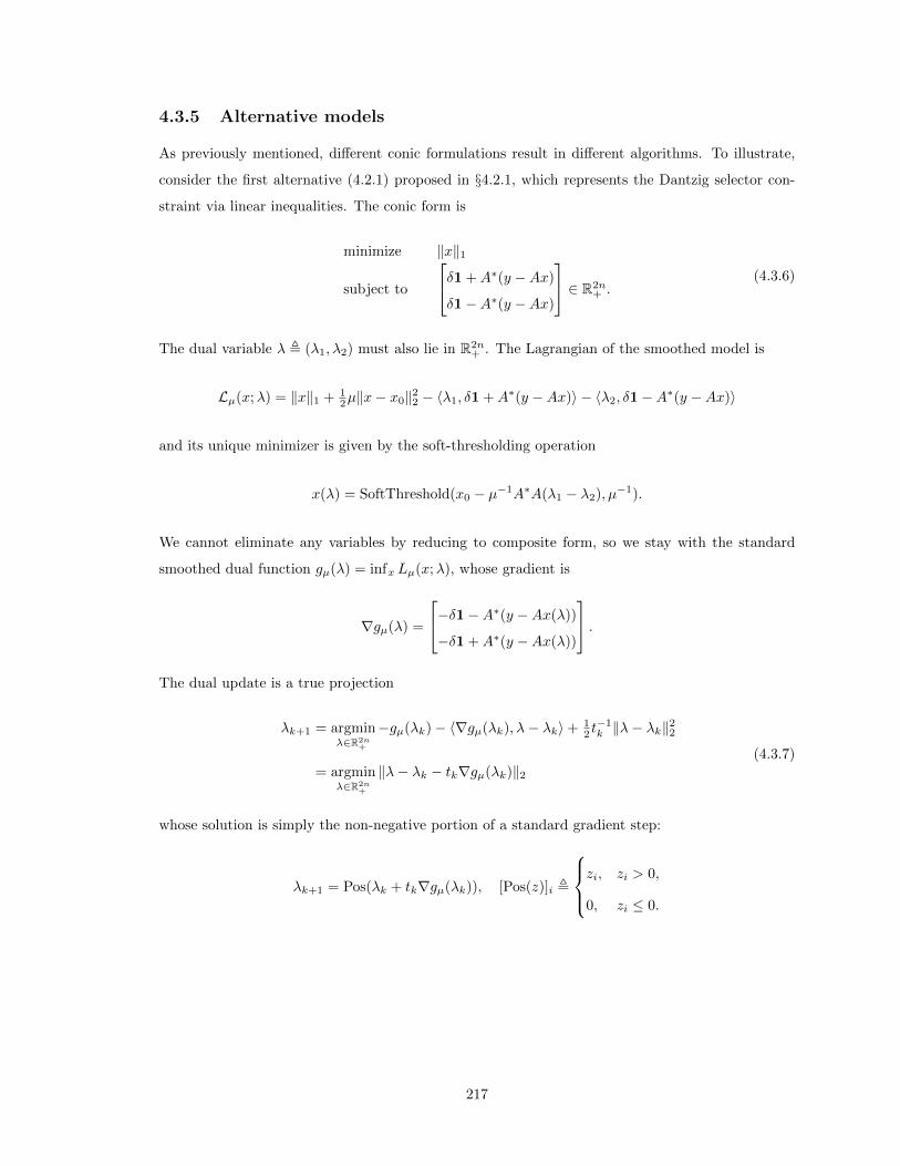
4.3.5 Alternative models

As previously mentioned, different conic formulations result in different algorithms. To illustrate,

consider the first alternative (4.2.1) proposed in §4.2.1, which represents the Dantzig selector con-

straint via linear inequalities. The conic form is

minimize ‖x‖1

subject to

δ1 +A∗(y −Ax)

δ1−A∗(y −Ax)

∈ R2n+ .

(4.3.6)

The dual variable λ , (λ1, λ2) must also lie in R2n+ . The Lagrangian of the smoothed model is

Lµ(x;λ) = ‖x‖1 + 12µ‖x− x0‖22 − 〈λ1, δ1 +A∗(y −Ax)〉 − 〈λ2, δ1−A∗(y −Ax)〉

and its unique minimizer is given by the soft-thresholding operation

x(λ) = SoftThreshold(x0 − µ−1A∗A(λ1 − λ2), µ−1).

We cannot eliminate any variables by reducing to composite form, so we stay with the standard

smoothed dual function gµ(λ) = infx Lµ(x;λ), whose gradient is

∇gµ(λ) =

−δ1−A∗(y −Ax(λ))

−δ1 +A∗(y −Ax(λ))

.The dual update is a true projection

λk+1 = argminλ∈R2n

+

−gµ(λk)− 〈∇gµ(λk), λ− λk〉+ 12 t−1k ‖λ− λk‖22

= argminλ∈R2n

+

‖λ− λk − tk∇gµ(λk)‖2(4.3.7)

whose solution is simply the non-negative portion of a standard gradient step:

λk+1 = Pos(λk + tk∇gµ(λk)), [Pos(z)]i ,

zi, zi > 0,

0, zi ≤ 0.

217

In order to better reveal the similarities between the two models, let us define z , λ1 − λ2 and

τ , 1∗(λ1 + λ2). Then we have ‖z‖1 ≤ τ , and the Lagrangian and its minimizer become

Lµ(x;λ) = ‖x‖1 + 12µ‖x− x0‖22 − 〈z, A∗(y −Ax)〉 − δτ ,

x(λ) = SoftThreshold(x0 − µ−1A∗Az, µ−1),

which are actually identical to the original norm-based model. The difference lies in the dual update.

It is possible to show that the dual update for the original model is equivalent to

zk+1 = Σ · argminλ∈R2n

+

−gµ(λk)− 〈∇gµ(λk), λ− λk〉+ 12 t−1k ‖Σ(λ− λk)‖22 (4.3.8)

for Σ = [+I,−I]. In short, the dual function is linear in the directions of λ1 + λ2, so eliminating

them from the proximity term would yield true numerical equivalence to the original model.

4.4 Further instantiations

Now that we have seen the mechanism for instantiating a particular instance of a compressed sensing

problem, let us show how the same approach can be applied to several other types of models.

Instead of performing the full, separate derivation for each case, we first provide a template for our

standard form. Then, for each specific model, we show the necessary modifications to the template

to implement that particular case.

4.4.1 A generic algorithm

A careful examination of our derivations for the Dantzig selector, as well as the developments in

§4.2.6, provide a clear path to generalizing Listing 1 above. We require implementations of the linear

operators A and its adjoint A∗, and values of the constants b, bτ ; recall that these are the partitioned

versions of A and b as described in §4.2.5. We also need to be able to perform the two-sequence

recursion (4.2.22), modified to include the step size multiplier θk and an adjustable centerpoint x0

in the proximity function.

Armed with these computational primitives, we present in Listing 2 a generic equivalent of the

algorithm employed for the Dantzig selector in Listing 1. It is important to note that this particular

variant of the optimal first-order methods may not be the best choice for every model; nevertheless

each variant uses the same computational primitives.

218

Listing 2 Generic algorithm for the conic standard form

Require: z0, x0 ∈ Rn, µ > 0, step sizes {tk}1: θ0 ← 1, v0 ← z0

2: for k = 0, 1, 2, . . . do

3: yk ← (1− θk)vk + θkzk

4: xk ← argminx f(x) + µd(x− x0)− 〈A∗(yk), x〉5: zk+1 ← argminz h(z) + θk

2tk‖z − zk‖2 + 〈A(xk) + b, z〉

6: vk+1 ← (1− θk)vk + θkzk+1

7: θk+1 ← 2/(1 + (1 + 4/θ2k)1/2)

In the next several sections, we show how to construct first-order methods for a variety of models.

We will do so by replacing lines 4–5 of Listing 2 with appropriate substitutions and simplified

expressions for each.

4.4.2 The LASSO

The conic form for the smoothed LASSO is

minimize ‖x‖1 + 12µ‖x− x0‖22

subject to (y −Ax, ε) ∈ Ln2 ,(4.4.1)

where Ln2 is the epigraph of the Euclidean norm. The Lagrangian is

Lµ(x; z, τ) = ‖x‖1 + 12µ‖x− x0‖22 − 〈z, y −Ax〉 − ετ.

The dual variable λ = (z, τ) is constrained to lie in the dual cone, which is also Ln2 . Eliminating τ

(assuming ε > 0) yields the composite dual form

maximize infx ‖x‖1 + 12µ‖x− x0‖22 − 〈z, y −Ax〉 − ε‖z‖2.

The primal projection with f(x) = ‖x‖1 is the same soft-thresholding operation used for the Dantzig

selector. The dual projection involving h(z) = ε‖z‖2, on the other hand, is

zk+1 = argminz

ε‖z‖2 + θk2tk‖z − zk‖22 + 〈x, z〉 = Shrink(zk − θ−1

k tkx, θ−1k tkε),

219

where x , y −Axk and Shrink is an `2-shrinkage operation

Shrink(z, t) , max{1− t/‖z‖2, 0} · z =

0, ‖z‖2 ≤ t,

(1− t/‖z‖2) · z, ‖z‖2 > t.

The resulting algorithm excerpt is given in Listing 3.

Listing 3 Algorithm excerpt for LASSO

4: xk ← SoftThreshold(x0 − µ−1A∗yk, µ−1)

5: zk+1 ← Shrink(zk − θ−1k tk(y −Axk), θ−1

k tkε)

4.4.3 Nuclear-norm minimization

Extending this approach to the nuclear-norm minimization problem

minimize ‖X‖∗subject to ‖y −A(X)‖2 ≤ ε

(4.4.2)

is straightforward. The composite smoothed dual form is

maximize infX ‖X‖∗ + µd(X)− 〈z, y −A(X)〉 − ε‖z‖2,

and the dual projection corresponds very directly to the LASSO. Choosing d(X) = 12‖X − X0‖2F

leads to a primal projection given by the soft-thresholding of singular values:

Xk = SoftThresholdSingVal(X0 − µ−1A∗(yk), µ−1). (4.4.3)

The SoftThresholdSingVal operation obeys [CCS10]

SoftThresholdSingVal(X, t) = U · SoftThreshold(Σ, t) · V ∗,

where X = UΣV ∗ is any singular value decomposition of Z, and SoftThreshold(Σ) applies soft-

thresholding to the singular values (the diagonal elements of Σ). This results in the algorithm

excerpt presented in Listing 4.

Listing 4 Algorithm for nuclear-norm minimization (LASSO constraint)

4: Xk ← SoftThresholdSingVal(X0 − µ−1A∗(yk), µ−1)

5: zk+1 ← Shrink(zk − θ−1k tk(y −A(Xk)), θ−1

k tkε)

220

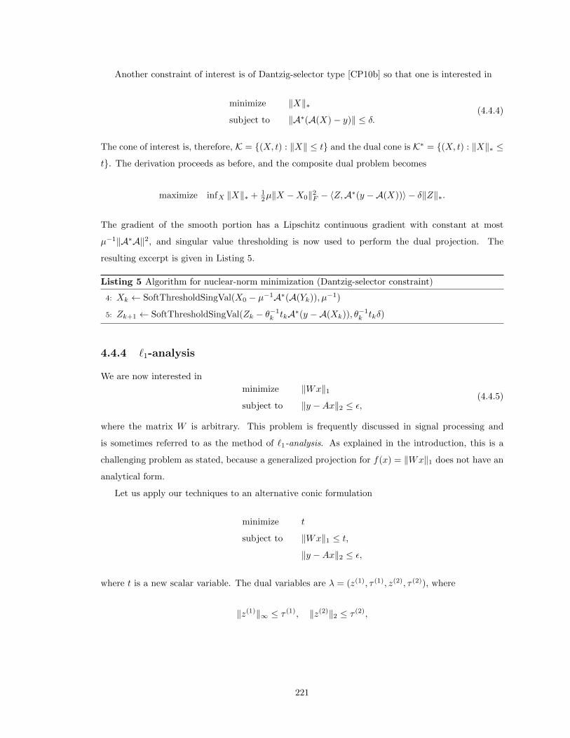
Another constraint of interest is of Dantzig-selector type [CP10b] so that one is interested in

minimize ‖X‖∗subject to ‖A∗(A(X)− y)‖ ≤ δ.

(4.4.4)

The cone of interest is, therefore, K = {(X, t) : ‖X‖ ≤ t} and the dual cone is K∗ = {(X, t) : ‖X‖∗ ≤t}. The derivation proceeds as before, and the composite dual problem becomes

maximize infX ‖X‖∗ + 12µ‖X −X0‖2F − 〈Z,A∗(y −A(X))〉 − δ‖Z‖∗.

The gradient of the smooth portion has a Lipschitz continuous gradient with constant at most

µ−1‖A∗A‖2, and singular value thresholding is now used to perform the dual projection. The

resulting excerpt is given in Listing 5.

Listing 5 Algorithm for nuclear-norm minimization (Dantzig-selector constraint)

4: Xk ← SoftThresholdSingVal(X0 − µ−1A∗(A(Yk)), µ−1)

5: Zk+1 ← SoftThresholdSingVal(Zk − θ−1k tkA∗(y −A(Xk)), θ−1

k tkδ)

4.4.4 `1-analysis

We are now interested in

minimize ‖Wx‖1subject to ‖y −Ax‖2 ≤ ε,

(4.4.5)

where the matrix W is arbitrary. This problem is frequently discussed in signal processing and

is sometimes referred to as the method of `1-analysis. As explained in the introduction, this is a

challenging problem as stated, because a generalized projection for f(x) = ‖Wx‖1 does not have an

analytical form.

Let us apply our techniques to an alternative conic formulation

minimize t

subject to ‖Wx‖1 ≤ t,‖y −Ax‖2 ≤ ε,

where t is a new scalar variable. The dual variables are λ = (z(1), τ (1), z(2), τ (2)), where

‖z(1)‖∞ ≤ τ (1), ‖z(2)‖2 ≤ τ (2),

221

and the Lagrangian is given by

L(x, t; z(1), τ (1), z(2), τ (2)) = t− 〈z(1),Wx〉 − τ (1)t− 〈z(2), y −Ax〉 − ετ (2).

The Lagrangian is unbounded unless τ (1) = 1; and we can eliminate τ (2) in our standard fashion as

well. These simplifications yield a dual problem

maximize 〈y, z(2)〉 − ε‖z(2)‖2subject to A∗z(2) −W ∗z(1) = 0,

‖z(1)‖∞ ≤ 1.

To apply smoothing to this problem, we use a standard proximity function d(x) = 12‖x − x0‖2.

(Setting τ (1) = 1 causes t to be eliminated from the Lagrangian, so it need not appear in our

proximity term.) The dual function becomes

gµ(z(1), z(2)) = infx

12µ‖x− x0‖22 − 〈z(1),Wx〉 − 〈z(2), y −Ax〉 − ε‖z(2)‖

and the minimizer x(z) is simply

x(z) = x0 + µ−1(W ∗z(1) −A∗z(2)).

Now onto the dual projection

zk+1 = argminz: ‖z(2)‖∞≤1

ε‖z(2)‖2 + θk2tk‖z − zk‖2 + 〈x, z〉,

where x = (Wx(z), y −Ax(z)). This will certainly converge if the step sizes tk are chosen properly.

However, if W and A have significantly different scaling, the performance of the algorithm may

suffer. Our idea is to apply different step sizes t(i)k to each dual variable

zk+1 = argminz: ‖z(2)‖∞≤1

ε‖z(2)‖2 + 〈x, z〉+ 12θk

2∑i=1

(t(i)k )−1‖z(i) − z(i)

k ‖22

in a fashion that preserves the convergence properties of the method. The minimization problem

over z is separable, and the solution is given by

z(1)k = Trunc(y

(1)k − θ−1

k t(1)k x(1), θ−1

k t(1)k ) (4.4.6a)

z(2)k = Shrink(y

(2)k − θ−1

k t(2)k x(2), θ−1

k t(2)k ε), (4.4.6b)

222

where the truncation operator is given element-wise by

Trunc(z, τ) = sgn(z) ·min{|z|, τ} =

z, |z| ≤ τ,

τ sgn(z), |z| ≥ τ.

In our current tests, we fix t(2)k = αt

(1)k , where we choose α = ‖W‖2/‖A‖2, or some estimate thereof.

This is numerically equivalent to applying a single step size to a scaled version of the original problem,

so convergence guarantees remain. In future work, however, we intend to develop a practical method

for adapting each step size separately.

The algorithm excerpt is given in Listing 6.

Listing 6 Algorithm excerpt for `1-analysis

4: xk ← x0 + µ−1(Wy(1)k −A∗y

(2)k )

5:z

(1)k+1 ← Trunc(y

(1)k − θ−1

k t(1)k Wxk, θ

−1k t

(1)k )

z(2)k+1 ← Shrink(y

(2)k − θ−1

k t(2)k (y −Axk), θ−1

k t(2)k ε)

4.4.5 Total-variation minimization

We now wish to solve

minimize ‖x‖TV

subject to ‖y −Ax‖2 ≤ ε(4.4.7)

for some image array x ∈ Rn2

where ‖x‖TV is the total-variation introduced in §4.1.1. We can

actually cast this as a complex `1-analysis problem

minimize ‖Dx‖1subject to ‖y −Ax‖2 ≤ ε

where D : Rn2 → C(n−1)2

is a matrix representing the linear operation that places horizontal and

vertical differences into the real and imaginary elements of the output, respectively:

[Dx]ij , (xi+1,j − xi,j) +√−1 · (xi,j+1 − xi,j), 1 ≤ i < n, 1 ≤ j < n.

Writing it in this way allows us to adapt our `1-analysis derivations directly. The smoothed dual

function becomes

gµ(z(1), z(2)) = infx

12µ‖x− x0‖22 − 〈z(1), Dx〉 − 〈z(2), y −Ax〉 − ε‖z(2)‖2,

223

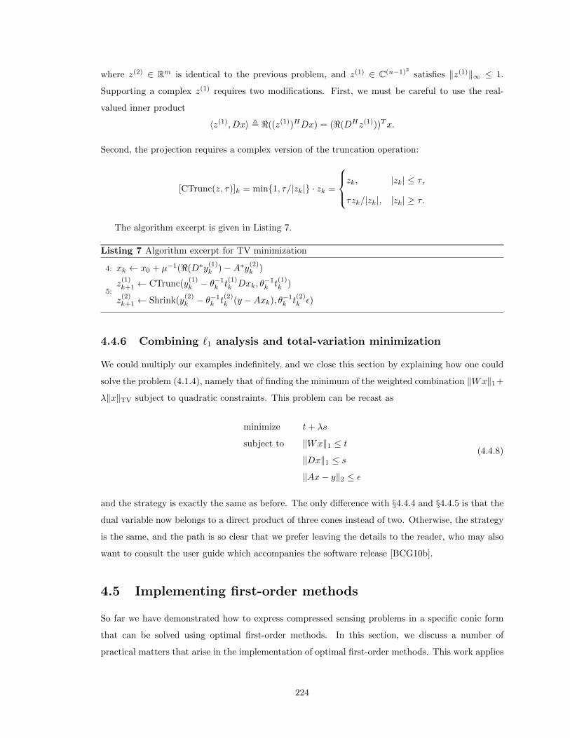
where z(2) ∈ Rm is identical to the previous problem, and z(1) ∈ C(n−1)2

satisfies ‖z(1)‖∞ ≤ 1.

Supporting a complex z(1) requires two modifications. First, we must be careful to use the real-

valued inner product

〈z(1), Dx〉 , <((z(1))HDx) = (<(DHz(1)))Tx.

Second, the projection requires a complex version of the truncation operation:

[CTrunc(z, τ)]k = min{1, τ/|zk|} · zk =

zk, |zk| ≤ τ,

τzk/|zk|, |zk| ≥ τ.

The algorithm excerpt is given in Listing 7.

Listing 7 Algorithm excerpt for TV minimization

4: xk ← x0 + µ−1(<(D∗y(1)k )−A∗y(2)

k )

5:z

(1)k+1 ← CTrunc(y

(1)k − θ−1

k t(1)k Dxk, θ

−1k t

(1)k )

z(2)k+1 ← Shrink(y

(2)k − θ−1

k t(2)k (y −Axk), θ−1

k t(2)k ε)

4.4.6 Combining `1 analysis and total-variation minimization

We could multiply our examples indefinitely, and we close this section by explaining how one could

solve the problem (4.1.4), namely that of finding the minimum of the weighted combination ‖Wx‖1+

λ‖x‖TV subject to quadratic constraints. This problem can be recast as

minimize t+ λs

subject to ‖Wx‖1 ≤ t‖Dx‖1 ≤ s‖Ax− y‖2 ≤ ε

(4.4.8)

and the strategy is exactly the same as before. The only difference with §4.4.4 and §4.4.5 is that the

dual variable now belongs to a direct product of three cones instead of two. Otherwise, the strategy

is the same, and the path is so clear that we prefer leaving the details to the reader, who may also

want to consult the user guide which accompanies the software release [BCG10b].

4.5 Implementing first-order methods

So far we have demonstrated how to express compressed sensing problems in a specific conic form

that can be solved using optimal first-order methods. In this section, we discuss a number of

practical matters that arise in the implementation of optimal first-order methods. This work applies

224

to a wider class of models than those presented in this chapter; therefore, we will set aside our conic

formulations and present the first-order algorithms in their more native form.

4.5.1 Introduction

The problems of interest in this chapter can be expressed in an unconstrained composite form

minimize φ(z) , g(z) + h(z), (4.5.1)

where g, h : Rn → (R∪+∞) are convex functions with g smooth and h non-smooth. (To be precise,

the dual functions in our models are concave, so we consider their convex negatives here.) Convex

constraints are readily supported by including their corresponding indicator functions into h.

First-order methods solve (4.5.1) with repeated calls to a generalized projection, such as

zk+1 ← argminz

g(zk) + 〈∇g(zk), z − zk〉+ 12tk‖z − zk‖2 + h(z), (4.5.2)

where ‖ · ‖ is a chosen norm and tk is the step size control. Proofs of global convergence depend

upon the right-hand approximation satisfying an upper bound property

φ(zk+1) ≤ g(zk) + 〈∇g(zk), zk+1 − zk〉+ 12tk‖zk+1 − zk‖2 + h(zk+1). (4.5.3)

This bound is certain to hold for sufficiently small tk; but to ensure global convergence, tk must be

bounded away from zero. This is typically accomplished by assuming that the gradient of g satisfies

a generalized Lipschitz criterion,

‖∇g(x)−∇g(y)‖∗ ≤ L‖x− y‖ ∀x, y ∈ domφ, (4.5.4)

where ‖ · ‖∗ is the dual norm; that is, ‖w‖∗ = sup{〈z, w〉 | ‖z‖ ≤ 1}. Then the bound (4.5.3) is

guaranteed to hold for any tk ≤ L−1. Under these conditions, convergence to ε accuracy—that

is, φ(zk) − infz φ(z) ≤ ε—is obtained in O(L/ε) iterations for a simple algorithm based on (4.5.2)

known variously as the forward-backward algorithm or proximal gradient descent, which dates to

at least [FM81]. This bound on the iterations improves to O(√L/ε) for the so-called optimal or

accelerated methods [Nes83,Nes88,Nes07,Tse08]. These optimal methods vary the calculation (4.5.2)

slightly, but the structure and complexity remain the same.

4.5.2 The variants

Optimal first-order methods have been a subject of much study in the last decade by many different

authors. In 2008, Tseng presented a nearly unified treatment of the most commonly cited methods,

225

and provided simplified proofs of global convergence and complexity [Tse08]; this paper was both

an aid and an inspiration for the modular template framework we present.

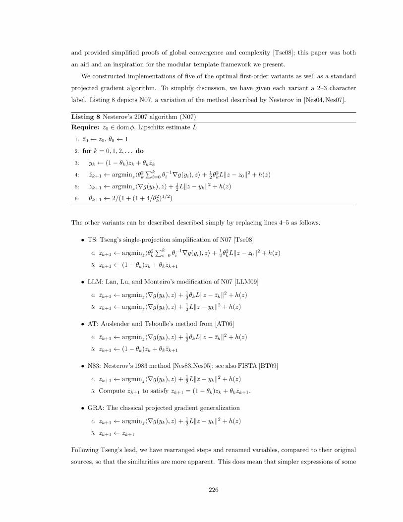
We constructed implementations of five of the optimal first-order variants as well as a standard

projected gradient algorithm. To simplify discussion, we have given each variant a 2–3 character

label. Listing 8 depicts N07, a variation of the method described by Nesterov in [Nes04,Nes07].

Listing 8 Nesterov’s 2007 algorithm (N07)

Require: z0 ∈ domφ, Lipschitz estimate L

1: z0 ← z0, θ0 ← 1

2: for k = 0, 1, 2, . . . do

3: yk ← (1− θk)zk + θkzk

4: zk+1 ← argminz〈θ2k

∑ki=0 θ

−1i ∇g(yi), z〉+ 1

2θ2kL‖z − z0‖2 + h(z)

5: zk+1 ← argminz〈∇g(yk), z〉+ 12L‖z − yk‖2 + h(z)

6: θk+1 ← 2/(1 + (1 + 4/θ2k)1/2)

The other variants can be described described simply by replacing lines 4–5 as follows.

• TS: Tseng’s single-projection simplification of N07 [Tse08]

4: zk+1 ← argminz〈θ2k

∑ki=0 θ

−1i ∇g(yi), z〉+ 1

2θ2kL‖z − z0‖2 + h(z)

5: zk+1 ← (1− θk)zk + θkzk+1

• LLM: Lan, Lu, and Monteiro’s modification of N07 [LLM09]

4: zk+1 ← argminz〈∇g(yk), z〉+ 12θkL‖z − zk‖2 + h(z)

5: zk+1 ← argminz〈∇g(yk), z〉+ 12L‖z − yk‖2 + h(z)

• AT: Auslender and Teboulle’s method from [AT06]

4: zk+1 ← argminz〈∇g(yk), z〉+ 12θkL‖z − zk‖2 + h(z)

5: zk+1 ← (1− θk)zk + θkzk+1

• N83: Nesterov’s 1983 method [Nes83,Nes05]; see also FISTA [BT09]

4: zk+1 ← argminz〈∇g(yk), z〉+ 12L‖z − yk‖2 + h(z)

5: Compute zk+1 to satisfy zk+1 = (1− θk)zk + θkzk+1.

• GRA: The classical projected gradient generalization

4: zk+1 ← argminz〈∇g(yk), z〉+ 12L‖z − yk‖2 + h(z)

5: zk+1 ← zk+1

Following Tseng’s lead, we have rearranged steps and renamed variables, compared to their original

sources, so that the similarities are more apparent. This does mean that simpler expressions of some

226

of these algorithms are possible, specifically for TS, AT, N83, and GRA. Note in particular that

GRA does not use the parameter θk.

Given their similar structure, it should not be surprising that these algorithms, except GRA,

achieve nearly identical theoretical iteration performance. Indeed, it can be shown that if z? is an

optimal point for (4.5.1), then for any of the optimal variants,

φ(zk+1)− φ(z?) ≤ 12Lθ

2k‖z0 − z?‖2 ≤ 2Lk−2‖z0 − z?‖2. (4.5.5)

Thus the number of iterations required to reach ε optimality is at most d√

2L/ε‖z0 − z?‖2e (again,

except GRA). Tighter bounds can be constructed in some cases but the differences remain small.

Despite their obvious similarity, the algorithms do have some key differences worth noting. First

of all, the sequence of points yk generated by the N83 method may sometimes lie outside of domφ.

This is not an issue for our applications, but it might be for those where g(z) may not be differentiable

everywhere. Secondly, N07 and LLM require two projections per iteration, while the others require

only one. Two-projection methods would be preferred only if the added cost results in a comparable

reduction in the number of iterations required. Theory does not support this trade-off, but the

results in practice may differ; see §4.7.1 for a single comparison.

4.5.3 Step size adaptation

All of the algorithms involve the global Lipschitz constant L. Not only is this constant often difficult

or impractical to obtain, the step sizes it produces are often too conservative, since the global

Lipschitz bound (4.5.4) may not be tight in the neighborhood of the solution trajectory. Reducing L

artificially can improve performance, but reducing it too much can cause the algorithms to diverge.

Our experiments suggest that the transition between convergence and divergence is very sharp.

A common solution to such issues is backtracking: replace the global constant L with a per-

iteration estimate Lk that is increased as local behavior demands it. Examining the convergence

proofs of Tseng reveals that the following condition is sufficient to preserve convergence (see [Tse08],

Propositions 1, 2, and 3):

g(zk+1) ≤ g(yk) + 〈∇g(yk), zk+1 − yk〉+ 12Lk‖zk+1 − yk‖2. (4.5.6)

If we double the value of Lk every time a violation of (4.5.6) occurs, for instance, then Lk will satisfy

Lk ≥ L after no more than dlog2(L/L0)e backtracks, after which the condition must hold for all

subsequent iterations. Thus strict backtracking preserves global convergence. A simple improvement

to this approach is to update Lk with max{2Lk, L}, where L is the smallest value of Lk that would

satisfy (4.5.6). To determine an initial estimate L0, we can select any two points z0, z1 and use the

227

formula

L0 = ‖∇g(z0)−∇g(z1)‖∗/‖z0 − z1‖.

Unfortunately, our experiments reveal that (4.5.6) suffers from severe cancellation errors when

g(zk+1) ≈ g(yk), often preventing the algorithms from achieving high levels of accuracy. More

traditional Armijo-style line search tests also suffer from this issue. We propose an alternative test

that maintains fidelity at much higher levels of accuracy:

|〈yk − zk+1,∇g(zk+1)−∇g(yk)〉| ≤ 12Lk‖zk+1 − yk‖22. (4.5.7)

It is not difficult to show that (4.5.7) implies (4.5.6), so provable convergence is maintained. It is a

more conservative test, however, producing smaller step sizes. So for best performance we prefer a

hybrid approach: for instance, use (4.5.6) when g(yk) − g(zk+1) ≥ γg(zk+1) for some small γ > 0,

and use (4.5.7) otherwise to avoid the cancellation error issues.

A closer study suggests a further improvement. Because the error bound (4.5.5) is proportional

to Lkθ2k, simple backtracking will cause it to rise unnecessarily. This anomaly can be rectified by

modifying θk as well as Lk during a backtracking step. Such an approach was adopted by Nesterov

for N07 in [Nes07]; and with care it can be adapted to any of the variants. Convergence is preserved

if

Lk+1θ2k+1/(1− θk+1) ≥ Lkθ2

k (4.5.8)

(see [Tse08], Proposition 1), which implies that the θk update in Line 6 of Listing 8 should be

θk+1 ← 2/(1 + (1 + 4Lk+1/θ2kLk)1/2). (4.5.9)

With this update the monotonicity of the error bound (4.5.5) is restored. For N07 and TS, the

update for zk+1 must also be modified as follows:

zk+1 ← argminz〈θ2kLk

∑ki=0(Liθi)

−1∇g(yi), z〉+ 12θ

2kLk‖z − z0‖2 + h(z). (4.5.10)

Finally, to improve performance we may consider decreasing the local Lipschitz estimate Lk

when conditions permit. We have chosen a simple approach: attempt a slight decrease of Lk at each

iteration; that is, Lk = αLk−1 for some fixed α ∈ (0, 1]. Of course, doing so will guarantee that

occasional backtracks occur. With judicious choice of α, we can balance step size growth for limited

amounts of backtracking, minimizing the total number of function evaluations or projections. We

have found that α = 0.9 provides good performance in many applications.

228

4.5.4 Linear operator structure

Let us briefly reconsider the special structure of our compressed sensing models. In these problems,

it is possible to express the smooth portion of our composite function in the form

g(z) = g(A∗(z)) + 〈b, z〉,

where g remains smooth, A is a linear operator, and b is a constant vector (see §4.2.5; we have

dropped some overbars here for convenience). Computing a value of g requires a single application

of A∗, and computing its gradient also requires an application of A. In many of our models, the

functions g and h are quite simple to compute, so the linear operators account for the bulk of the

computational costs. It is to our benefit, then, to utilize them as efficiently as possible.

For the prototypical algorithms of Section 4.5.2, each iteration requires the computation of the

value and gradient of g at the single point yk, so all variants require a single application each of Aand A∗. The situation changes when backtracking is used, however. Specifically, the backtracking

test (4.5.6) requires the computation of g at a cost of one application of A∗; and the alternative test

(4.5.7) requires the gradient as well, at a cost of one application of A. Fortunately, with a careful

rearrangement of computations we can eliminate both of these additional costs for single-projection

methods TS, AT, N83, and GRA, and one of them for the two-projection methods N07 and LLM.

Listing 9 AT variant with improved backtracking

Require: z0 ∈ domφ, L > 0, α ∈ (0, 1], β ∈ (0, 1)1: z0 ← z0, zA0, zA0 ← A∗(z0), θ−1 = +∞, L−1 = L2: for k = 0, 1, 2, . . . do3: Lk ← αLk−1

4: loop5: θk ← 2/(1 + (1 + 4Lk/θ

2k−1Lk−1)1/2) (θ0 , 1)

6: yk ← (1− θk)zk + θkzk, yA,k ← (1− θk)zA,k + θkzA,k7: gk ← ∇g(yA,k), gk ← Agk + b8: zk+1 ← argminz〈gk, z〉+ h(z) + θk

2tk‖z − yk‖2, zA,k+1 ← A∗(zk+1)

9: zk+1 ← (1− θk)zk + θkzk+1, zA,k+1 ← (1− θk)zA,k + θkzA,k10: L← 2 |〈yA,k − zA,k+1,∇g(zA,k+1)− gk〉| /‖zk+1 − yk‖2211: if Lk ≥ L then break endif12: Lk ← max{Lk/β, L}

Listing 9 depicts this more efficient use of linear operators, along with the step size adaptation

approach, using the AT variant. The savings come from two different additions. First, we maintain

additional sequences zA,k and zA,k to allow us to compute yA,k = A∗(yk) without a call to A∗.Secondly, we take advantage of the fact that

〈yk − zk+1,∇g(zk+1)−∇g(yk)〉 = 〈yA,k − zA,k+1,∇g(zA,k+1)−∇g(yA,k)〉,

229

which allows us to avoid having to compute the full gradient of g; instead we need to compute only

the significantly less expensive gradient of g.

4.5.5 Accelerated continuation

Several recent algorithms, such as FPC and NESTA [HYZ08, BBC11], have empirically found that

continuation schemes greatly improve performance. The idea behind continuation is that we solve the

problem of interest by solving a sequence of similar but easier problems, using the results of each sub-

problem to initialize or warm start the next one. Listing 10 below depicts a standard continuation

loop for solving the generic conic problem in (4.1.14) with a proximity function d(x) = 12‖x− x0‖22.

We have used a capital X and loop count j to distinguish these iterates from the inner loop iterates

xk generated by a first-order method.

Listing 10 Standard continuation

Require: Y0, µ0 > 0, β < 1

1: for j = 0, 1, 2, . . . do

2: Xj+1 ← argminA(x)+b∈K f(x) +µj2 ‖x− Yj‖22

3: Yj+1 ← Xj+1 or Yj+1 ← Yj

4: µj+1 ← βµj

Note that Listing 10 allows for the updating of both the smoothing parameter µj and the prox-

imity center Yj at each iteration. In many implementations, Yj ≡ X0 and only µj is decreased, but

updating Yj as well will almost always be beneficial. When Yj is updated in this manner, the algo-

rithm is known as the proximal point method, which has been studied since at least [Roc76]. Indeed,

one of the accelerated variants [AT06] that is used in our solvers uses the proximal point framework

to analyze gradient-mapping type updates. It turns out we can do much better by applying the

same acceleration ideas already mentioned.

Let us suggestively write

h(Y ) = minx∈C

f(x) +µ

2‖x− Y ‖22, (4.5.11)

where µ > 0 is fixed and C is a closed convex set. This is an infimal convolution, and h is known as

the Moreau-Yosida regularization of f [HUL93]. Define

XY = argminx∈C

f(x) +µ

2‖x− Y ‖22. (4.5.12)

The map Y 7→ XY is a proximity operator [Mor65].

We now state a very useful theorem.

230

Theorem 4.5.1. The function h (4.5.11) is continuously differentiable with gradient

∇h(Y ) = µ(Y −XY ). (4.5.13)

The gradient is Lipschitz continuous with constant L = µ. Furthermore, minimizing h is equivalent

to minimizing f(x) subject to x ∈ C.

The proof is not difficult and can be found in Proposition I.2.2.4 and §XV.4.1 in [HUL93]; see

also exercises 2.13 and 2.14 in [BNO03], where h is referred to as the envelope function of f . The

Lipschitz constant is µ since XY is a proximity operator P , and I − P is non-expansive for any

proximity operator.

The proximal point method can be analyzed in this framework. Minimizing h using gradient

descent, with step size t = 1/L = 1/µ, gives

Yj+1 = Yj − t∇h(Yj) = Yj −1

µµ(Yj −XYj ) = XYj ,

which is exactly the proximal point algorithm. But since h has a Lipschitz gradient, we can use the

accelerated first-order methods to achieve a convergence rate of O(j−2), versus O(j−1) for standard

continuation. In Listing 11, we offer such an approach using a fixed step size t = 1/L and the

accelerated algorithm from Algorithm 2 in [Tse08]. This accelerated version of the proximal point

algorithm has been analyzed in [G92] where it was shown to be stable with respect to inexact solves.

Listing 11 Accelerated continuation

Require: Y0, µ0 > 0

1: X0 ← Y0

2: for j = 0, 1, 2, . . . do

3: Xj+1 ← argminA(x)+b∈K f(x) +µj2 ‖x− Yj‖22

4: Yj+1 ← Xj+1 + jj+3 (Xj+1 −Xj)

5: (optional) increase or decrease µj

Figure 4.3 provides an example of the potential improvement offered by accelerated continuation.

In this case, we have constructed a LASSO model with a 80 × 200 i.i.d. Gaussian measurement

matrix. The horizontal axis gives the number of continuation steps taken, and the vertical axis

gives the error ‖Xj − x?‖2/‖x?‖2 between each continuation iterate and an optimal solution to

the unsmoothed model; empirically, the optimal solution appears to be unique. Both simple and

accelerated continuation have been employed, using a fixed smoothing parameter µj ≡ µ0.8 A clear

advantage is demonstrated for accelerated continuation in this case.

8If µ is fixed, this is not continuation per se, but we still use the term since it refers to an outer iteration.

231

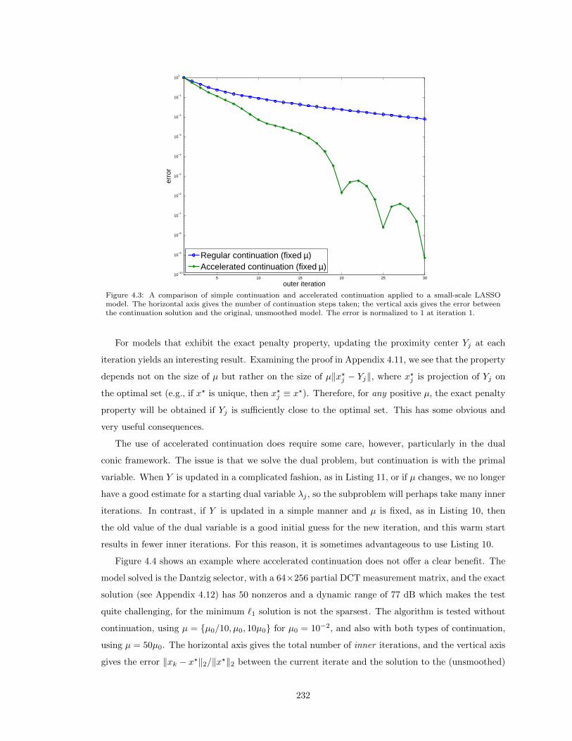
5 10 15 20 25 3010

−10

10−9

10−8

10−7

10−6

10−5

10−4

10−3

10−2

10−1

100

outer iteration

erro

r

Regular continuation (fixed µ)Accelerated continuation (fixed µ)

Figure 4.3: A comparison of simple continuation and accelerated continuation applied to a small-scale LASSOmodel. The horizontal axis gives the number of continuation steps taken; the vertical axis gives the error betweenthe continuation solution and the original, unsmoothed model. The error is normalized to 1 at iteration 1.

For models that exhibit the exact penalty property, updating the proximity center Yj at each

iteration yields an interesting result. Examining the proof in Appendix 4.11, we see that the property

depends not on the size of µ but rather on the size of µ‖x?j − Yj‖, where x?j is projection of Yj on

the optimal set (e.g., if x? is unique, then x?j ≡ x?). Therefore, for any positive µ, the exact penalty

property will be obtained if Yj is sufficiently close to the optimal set. This has some obvious and

very useful consequences.

The use of accelerated continuation does require some care, however, particularly in the dual

conic framework. The issue is that we solve the dual problem, but continuation is with the primal

variable. When Y is updated in a complicated fashion, as in Listing 11, or if µ changes, we no longer

have a good estimate for a starting dual variable λj , so the subproblem will perhaps take many inner

iterations. In contrast, if Y is updated in a simple manner and µ is fixed, as in Listing 10, then

the old value of the dual variable is a good initial guess for the new iteration, and this warm start

results in fewer inner iterations. For this reason, it is sometimes advantageous to use Listing 10.

Figure 4.4 shows an example where accelerated continuation does not offer a clear benefit. The

model solved is the Dantzig selector, with a 64×256 partial DCT measurement matrix, and the exact

solution (see Appendix 4.12) has 50 nonzeros and a dynamic range of 77 dB which makes the test

quite challenging, for the minimum `1 solution is not the sparsest. The algorithm is tested without

continuation, using µ = {µ0/10, µ0, 10µ0} for µ0 = 10−2, and also with both types of continuation,

using µ = 50µ0. The horizontal axis gives the total number of inner iterations, and the vertical axis

gives the error ‖xk − x?‖2/‖x?‖2 between the current iterate and the solution to the (unsmoothed)

232

0 1000 2000 3000 4000 5000 6000 7000 8000 9000 1000010

−10

10−8

10−6

10−4

10−2

100

iterations

erro

r

no continuation, µ/10no continuation, µno continuation, 10 µregular continuationaccelerated continuation

Figure 4.4: Comparing fixed smoothing and continuation strategies for a Dantzig selector model. The horizontalaxis gives the number of inner iterations of each first-order method. For the two continuation strategies, the circlesdepict the completion of each continuation step.

model. When no continuation is employed, the trade-off between solution accuracy (small µ) and

the number of iterations to converge (large µ) is evident. Continuation helps drastically, and high

levels of accuracy can be obtained quickly. In this example, both forms of continuation perform

similarly.

In our experience, accelerated continuation usually matches or outperforms regular continuation,

but the matter requires further study. In particular, performance is affected by the stopping criteria

of the inner iteration, and we plan to investigate this in future work. The experiments in Figure 4.4

decreased the tolerance by a factor of two every iteration, with the exception of the final iteration

which used a stricter tolerance.

4.5.6 Strong convexity

Suppose that our composite function φ is strongly convex; that is,

φ(z) ≥ φ(z0) + 12mφ‖z − z0‖22 ∀z ∈ domφ

for some fixed mφ > 0. It is well known that a standard gradient method will achieve linear

convergence in such a case. Unfortunately, without modification, none of the so-called optimal

methods will do so. Thus in the presence of strong convexity, standard gradient methods can

actually perform better than their so-called optimal counterparts.

If the strong convexity parameter mφ ≤ Lφ is known or can be bounded below, the N83 al-

gorithm can be modified to recover linear convergence [Nes05, Nes07], and will recover its superior

233

0 500 1000 1500 2000 2500 3000

10−12

10−10

10−8

10−6

10−4

10−2

100

iterations

erro

r

GRA, backtrackingAT, backtrackingAT, restart every 5AT, restart every 10AT, restart every 50AT, restart every 100N83, using m

Figure 4.5: First-order methods applied to a strongly convex problem: GRA, AT without restart, AT with restart,and N83 tuned with knowledge of the strong convexity parameter. The y-axis is ‖xk − x?‖2/‖x?‖2.

performance compared to standard gradient methods. The challenge, of course, is that this param-

eter rarely is known. In [Nes07], Nesterov provides two approaches for dealing with the case of

unknown mφ, one of which is readily adapted to all of the first-order variants here. That approach is

a so-called restart method: the algorithm is restarted after a certain number of iterations, using the

current iterate as the starting point for the restart; or, equivalently, the acceleration parameter θk is

reset to θ0 = 1. In theory, the optimal number of iterations between restarts depends on mφ/Lφ, but

linear convergence can be recovered even for sub-optimal choices of this iteration count [GLW09].

To illustrate the impact of strong convexity on performance, we constructed a strongly quadratic

unconstrained function with mφ = 0.07 and Lφ = 59.1, and minimized it using the gradient method

(GRA), the AT first-order method with and without restart, and the N83 method tuned to the

exact values of (mφ, Lφ). Backtracking was employed in all cases; we have verified experimentally

that doing so consistently improves performance and does not compromise the exploitation of strong

convexity. As can be seen in Figure 4.5, while AT without restart initially performs much better than

GRA, the linear convergence obtained by GRA will eventually overtake it. The N83 method is clearly

superior to either of these, achieving linear convergence with a much steeper slope. When restart is

employed, AT recovers linear convergence, and achieves near parity with N83 when restarted every

100 iterations (the optimal value predicted by [GLW09] is every 112 iterations).

The benefits of exploiting strong convexity seem clearly established. In fact, while proofs of

linear convergence assume global strong convexity, our experiments in §4.7 show that applying

234

these methods to models with local strong convexity can improve performance as well, sometimes

significantly. Unfortunately, the restart method requires manual tuning on a case-by-case basis to

achieve the best performance. This is certainly acceptable in many applications, but further research

is needed to develop approaches that are more automatic.

4.6 Dual-function formulation

Instead of a conic viewpoint, where the main requirement was the ability to project onto a cone

(often an epigraph cone), we may also view the problem in a dual function framework. The resulting

algorithm is identical; the new derivation is presented because it may be more natural for some

problems. A similar framework is presented in [CDV10], which uses proximal splitting methods

instead of gradient-based methods.

4.6.1 Background

In this section, convex functions are allowed to take values in (−∞,+∞]. The domain of a convex

function f is the set of points dom f = {x : f(x) < +∞} and the epigraph is epi f = {(x, η) : f(x) ≤η}. A convex function is proper if it is not the constant function f = +∞, and it is called lower

semi-continuous (lsc) if epi f is closed. Let Γ0(Rn) be the set of proper, lsc, convex functions f on

Rn. As a shorthand, we write “f is convex” to mean f ∈ Γ0(Rn), since we will not discuss convex

functions that are not in Γ0. If the reader is not familiar with subgradients and standard convex

analysis, then [Roc70] is recommended as the classic reference, or [BC11] for a modern perspective.

The convex dual function (also known as the Fenchel or Fenchel-Legendre dual) of a convex

function f is given by:

f∗(z) = supx〈z, x〉 − f(x).

The dual f∗ is also convex, and since f is lsc, f∗∗ = f .

We re-introduce the Moreau proximity operator [Mor62, Mor65] (first discussed in §4.5.5) using

slightly different notation. This Moreau proximity operator is also known as a proximity func-

tion, or a “proximation” in [Roc70], and the Moreau envelope is also known as the Moreau-Yosida

regularization.

Definition 4.6.1 (Moreau proximity operator). The Moreau envelope of a convex function f is

ef (z) = minx

f(x) +1

2‖x− z‖22 (4.6.1)

235

and the Moreau proximity operator

proxf (z) = argminx

f(x) +1

2‖x− z‖22. (4.6.2)

Define

ef,µ(z) = argminx

f(x) +µ

2‖x− z‖22

and define proxf,µ analogously.

Theorem 4.5.1 shows ef,µ(z) is continuously differentiable with gradient

∇zef,µ(z) = µ(z − proxf,µ(z)). (4.6.3)

and Lipschitz constant µ.

The classical orthogonal projection theorem states that for any subspace V ⊂ Rn, then x ∈ Rn

can be decomposed x = x‖ + x⊥ where x‖ ∈ V and 〈x‖, x⊥〉 = 0. Using the Moreau proximity

operator, it is possible to prove a more general projection theorem which includes the classical

projection theorem as a subcase.

Lemma 4.6.2 (Moreau’s decomposition [CW05]). Let f be a convex function, x ∈ Rn, and µ > 0.

Then

x = x‖ + x⊥ where (4.6.4)

x‖ = µproxf,µ−1(x), x⊥ = proxf∗,µ(x/µ) (4.6.5)

and f(x‖) + f∗(x⊥/µ) = µ−1〈x‖, x⊥〉. (4.6.6)

If particular, if µ = 1, then

x‖ = proxf (x), x⊥ = proxf∗(x), f(x‖) + f∗(x⊥) = 〈x‖, x⊥〉.

4.6.2 Fenchel dual formulation

Consider the problem

minxf(x) +

µ

2‖x− x0‖2 +

K∑i=1

φi(Aix+ bi) (4.6.7)

where f and φi are convex functions. This allows the case when φi may be the indicator function ι

to a set C:

ιC(x) =

0 x ∈ C

+∞ x /∈ C.

236

The set C must be closed in order for f = ιC to be lsc. We apply the dual formulation to (4.6.7).

The first step is introducing slack variables yi = Aix+ bi, so that (4.6.7) is equivalent to

minx,yi

f(x) +µ

2‖x− x0‖2 +

K∑i=1

φi(yi) such that yi = Aix+ bi ∀i ≤ K. (4.6.8)

Let z(λ) = µ−1∑iA

Ti λi, where λi ∈ Rmi if Ai ∈ Rmi×n, and λ represents λ1, . . . , λK . The dual

function is

g(λ) = infx,yi

(f(x) +

µ

2‖x− x0‖2 +

∑i

φi(y) + 〈λi, Aix+ bi − yi〉)

=∑i

〈λi, bi〉+ infx

(f(x) +

µ

2‖x− x0‖2 + µ〈z(λ), x〉

)+∑i

infyi

(φ(yi)− 〈λi, yi〉)

=∑i

〈λi, bi〉 −µ

2‖z(λ)‖2 + µ〈z(λ), x0〉+ inf

x

(f(x) +

µ

2‖x− (x0 − z(λ))‖2

)−∑i

φ∗(λi)

=∑i

〈λi, bi〉 −µ

2‖z(λ)‖2 + µ〈z(λ), x0〉+ ef,µ(x0 − z(λ))︸ ︷︷ ︸

gsmooth(λ)

−∑i

φ∗(λi)︸ ︷︷ ︸h(λ)

. (4.6.9)

The dual function is always concave. Using (4.6.3),

∇λigsmooth(λ) = bi +Aix(λ), x(λ) = proxf,µ(x0 − z(λ)).

Let A = [A1;A2; . . . ;AK ] and b = [b1; b2; . . . ; bK ] (both with∑Ki=1mi rows), then the total deriva-

tive is

∇λgsmooth(λ) = b +Ax(λ).

Since x(λ) is computed via a proximity operator, it is a non-expansive function of its inputs x0−z(λ),

where z(λ) = µ−1ATλ, so ∇gsmooth is Lipschitz continuous with bound

L = µ−1‖AAT ‖ ≤ µ−1K∑i=1

‖ATi Ai‖.

If, say, ‖AT1 A1‖ is very large but ‖AT2 A2‖ is small, then the Lipschitz bound is large and the λ2

variable will converge slowly due to the presence of the variable λ1 with a very different scale. It is

best if all λi have the same scale. This can be enforced by introducing the scaling αi = ‖ATi Ai‖−1/2,

and modifying (4.6.8) as follows:

minx,yi

f(x) +µ

2‖x− x0‖2 +

K∑i=1

φi(yi) such that yi = α−1i (Aix+ bi) ∀i ≤ K

237

and φi(y) = φi(αiy). Computing the proximity operator of φi is no more difficult than computing

the proximity operator of φi. From now on, we assume this scaling has already been performed.

The dual problem is

maxλi,i=1,...,K

gsmooth(λ)− h(λ) (4.6.10)

The dual function is an unconstrained problem (other than any implicit constraints in φ∗), and

it can be solved with the composite formulation previously discussed. The composite formulation

requires the gradient of gsmooth and the ability to solve the generalized projection with h; the

generalized projection can be rewritten in terms of the Moreau proximity function of h. Furthermore,

this is separable in λi. Thus (4.6.10) is easy to solve when

1. proxf is efficient to calculate, and

2. proxφ∗i is efficient to calculate for all i.

For many functions, such as norms, the proximity operator is O(n) to compute. For a list of functions

with known proximity operators, see [CW05].

There are three especially salient points:

1. φ∗i is the dual function of φi(x), and not the dual function of φi(x) ≡ φi(Aix + b). The dual

function of φi may be much more difficult to compute. This is the same observation made

earlier that it is easy to project onto the set {x : ‖x‖2 ≤ 1} but it can be difficult to project

onto the set {x : ‖Ax‖2 ≤ 1}. This observation has been made many times in the history of

optimization; see, for example, the discussion of Uzawa’s algorithm in [Cia89].

2. Using Moreau’s decomposition (4.6.4) and (4.6.5), it’s clear that computing proxf and proxf∗

are equally easy or difficult, since one can be computed via the other.

3. It is possible to define φK+1 ← f , AK+1 ← I, bK+1 ← 0, and f ← 0. That is, f can be

treated specially and kept in the primal, or we can introduce one more dual variable λK+1 and

think of f as another φi. The result algorithms are different, although they will solve the same

problem at convergence. The complexity per iteration stays nearly the same since proxf∗ has

the same cost as proxf , and the proximity operator of the zero function is trivial to compute.

We note that the convergence properties of the two methods need not be the same, but one

version may sometimes be used to bound the convergence of the other, as we show in §4.6.3.2.

This dual-function viewpoint is especially useful for problems considered in this chapter, since f

and φi are typically norms or indicator functions of norm balls. Define the dual norm of any norm

‖ · ‖ to be ‖ · ‖∗ where

‖y‖∗ , sup‖x‖≤1

〈y, x〉.

238

Then

h(y) = s‖y‖ ⇐⇒ h∗(z) = ι{z:‖z‖∗≤s}. (4.6.11)

If projection onto the dual-norm ball is efficient, then the dual smoothing algorithm has cheap per-

iteration cost. Many signal processing problems involve only the `1, `2, and `∞ norms, for which

projection onto the norm ball is O(n) or O(n log n), and hence any minimization problem with

convex combinations of these norms (with possibly affine scalings) is cheap to solve.

4.6.3 Convergence

Via the dual-function framework, it is possible to prove the convergence rate of the algorithm. There

are three major steps: first, we show in §4.6.3.1 that the iterates xk converge when solving a special

variant of (4.6.7). Secondly, §4.6.3.2 extends this to cover the generic case, and thirdly, in §4.6.4.1

we incorporate continuation and prove that the value of the outer function converges.

4.6.3.1 Convergence when f is smooth

The problem in (4.6.7) allows a number of functions φi, but for simplicity let us restrict to the case

of K = 1, so the problem of interest is

minxf(x) +

µ

2‖x− x0‖2 + φ1(Ax+ b). (4.6.12)

As discussed above, it is possible to treat f as one of the φi, e.g.,

minx

0 +µ

2‖x− x0‖2 + φ1(y1) + φ2(y2) such that y1 = Ax+ b, y2 = x (4.6.13)

where φ2(x) = f(x). In this case, gsmooth is a quadratic function, so it is both smooth and strongly

convex (with parameter µ). The dual function is

g(λ1, λ2) = gsmooth(λ1, λ2)− φ∗1(λ1)− φ∗2(λ2)

and x(λ) is a linear function of λ1 and λ2.

When solving the dual problem via an accelerated method, the dual objective converges at the

rate

g? − g(λ) ≤ Cµ−1

k2.

While the objective value converges, the dual variable λ need not converge, and there may not be a

unique maximizer λ?.

Since we now think of f as φ2, which acts as a “constraint” in a generalized projected-gradient

algorithm, the primal objective function is just the smoothing term µ2 ‖x − x0‖2, which is strongly

239

convex. Hence it is not unreasonable to expect that the primal variable x does converge. Indeed,

this is the case. A recent result in [FP11], using a Bregman distance technique, gives

‖x(λk)− x?‖2 ≤ 2

µ(g? − g(λk)). (4.6.14)

See Theorem 1 and Theorem 2 in [FP11]; it is also mentioned in [CP10c].

A broad class of models, such as solving the `1-analysis problem and TV-minimization, fall into

this category, so this result is useful in itself.

4.6.3.2 Convergence of inner iteration

Consider again (4.6.12). It seems unlikely that convergence is dependent on the “interpretation” of

f , so we are inclined to believe that the model

minxf(x) +

µ

2‖x− x0‖2 + φ1(y1) such that y1 = Ax+ b (4.6.15)

should converge at the same rate. This intuition is correct, and we show how to obtain the bound.

Using the special case just discussed in (4.6.13) (refer to this as case “A”), the dual function

depends on λ1 and λ2. Write this dual function as gA:

gA(λ1, λ2) = infxLA(λ1, λ2, x) = LA(λ1, λ2, xA(λ)) (4.6.16)

LA(λ1, λ2, x) = 〈λ1, b1〉+(

0 +µ

2‖x− x0‖2 + 〈ATλ1 + λ2, x〉

)− φ∗1(λ1)− f∗(λ2)

xA(λ) = argminx

µ

2‖x− x0‖2 + 〈ATλ1 + λ2, x〉. (4.6.17)

Using the new case (4.6.15) (case “B”), we keep f in primal form, and the dual function, written

as gB to distinguish it from the other case, is only a function of λ1:

gB(λ1) = infxLA(λ1, x) = LB(λ1, xB(λ)) (4.6.18)

LB(λ1, x) = 〈λ1, b1〉+(f(x) +

µ

2‖x− x0‖2 + 〈ATλ1, x〉

)− φ∗1(λ1)

xB(λ) = argminx

f(x) +µ

2‖x− x0‖2 + 〈ATλ1, x〉. (4.6.19)

Our strategy is as follows. Solve “B” and bound the objective g? − gB(λ1) ≤ C (using standard

convergence results on Nesterov’s method and variants) for some λ1 (really, this is λ(k)1 since it

depends on the iteration, but we drop the dependence on k for simplicity). Using λ1, we generate

λ2 so that xA(λ1, λ2) = xB(λ1) and gA(λ1, λ2) = gB(λ1). Thus we can apply existing results from

the previous section that give us the bound on xA, and hence xB , in terms of g? − gA(λ1, λ2) ≤ C.

We start with a known λ1 and xB calculated via method “B”. In the proximity calculation

240

(4.6.19), we know that xB must satisfy the first-order condition

0 ∈ ∂f(xB) + µ(xB − x0) +ATλ1.

Define

λ2 = −µ(xB − x0)−ATλ1,

so λ2 ∈ ∂f(xB). By examining (4.6.17) with this value of λ2 (and the same value of λ1), it’s clear

that xA = xB , since (4.6.17) is the minimization of an unconstrained differentiable function and has

a unique minimizer characterized by

0 = λ2 + µ(xA − x0) +ATλ1

which is certainly also satisfied by xB .

The remaining question is whether LA(λ1, λ2, xB) = LB(λ1, xB). This is verified by an applica-

tion of Fenchel’s equality [Roc70]

LB(λ1, xB)− LA(λ1, λ2, xB) = f(xB)− 〈λ2, xB〉+ f∗(λ2)

= 0

since λ2 ∈ ∂f(xB). Hence any sequence generated by method “B” has the same bounds that method

“A” enjoys.

4.6.4 Convergence of outer iteration

Let F (x) = f(x) +∑i φi(Aix+ bi), so the primal problem is

minxF (x).

The accelerated continuation scheme solves this by solving a problem of the form

minY

minxF (x) +

µ

2‖x− Y ‖2︸ ︷︷ ︸

ψ(Y )

(4.6.20)

by using the method in Listing 11. When the outer iteration uses an accelerated method, we call this

the accelerated proximal point algorithm; if the outer iteration is gradient descent with fixed step

size, this reduces to the proximal point algorithm. Let ψj = ψ(Yj) be the value of the outer iteration

at step j. If ψj is known exactly, then because accelerated continuation is an optimal method, the

value of ψ will converge to the optimal value ψ(Y ?) at rate O( µj2 ).

241

The calculation of ψj is done with an inner iteration, and this will never be exact. The inner

iteration is solved in the dual smoothing framework, and so the dual function g(λk) converges to

g(λ?j ) = minF (x) + µ2 ‖x − Yj‖2 at rate O(µ

−1

k2 ). There is a trade off in the value of µ, since a

small µ will speed up the outer iteration but slow down the inner iteration; it is also possible to

vary µ every outer-iteration. Is it possible to make precise this trade off, and thus suggest the best

value of µ to use? To what accuracy should the sub-problems be solved? On linear programs, does

this accelerated proximal-point algorithm converge in a finite number of iterations, as the regular

proximal-point algorithm does [PT74, Ber75]? Using very recent results, we begin to answer these

questions in §4.6.3 and §4.6.4.1; this work has not appeared in the preprint version of this chapter.

Below, we review existing results, and set the stage for the final convergence proof.

In 1992, Guler [G92] analyzed an accelerated variant of the proximal point algorithm and provided

the first robust convergence analysis. Let X?j = argminF (x) + µ/2‖x − Yj‖2. Guler proved that if

every inner iteration is solved to an iterate xk satisfying an inexact criteria, it can still be possible to

recovery accelerated convergence. In the case F is a Lipschitz function and finite, then his inexact

criteria simplifies to

‖xk −X?j ‖2 ≤

C

j1.5(4.6.21)

and still guarantees that the outer iteration converges in O(µ/j2). His variant of the accelerated

first-order method is not identical to the accelerated continuation scheme we present, but it is trivial

to adapt the accelerated continuation to use his version.

A recent paper by Combettes et al. [CDV10] considers a similar problem and proves convergence

of a similar scheme but using splitting methods instead of gradient-based methods, and does not

obtain any convergence rate bounds. Using the special form of a smoothed problem like ours,

[CDV10] shows that a bound on either ‖λk − λ?j‖, or ‖∇gsmooth(λk)−∇gsmooth(λju?)‖ is sufficient

to bound ‖xk − X?j ‖. The accelerated composite methods used to solve the dual will guarantee

that the generalized gradient mapping converges, but this does not imply that ∇gsmooth converges.

For unconstrained dual problems, such as noiseless basis pursuit and noiseless matrix completion,

the generalized gradient mapping is just the gradient, and hence we can bound the rate at which

xk → X?j for these specific problems. This result covers some previously known special cases.

For example, [COS09] proves convergence of linear Bregman and provides a rate of convergence;

linear Bregman is the same as our dual smoothing approach applied to noiseless basis pursuit, with

x0 = 0 and using fixed step-size gradient descent. The work of [MZ09] considers a situation similar

to [CDV10] but does not prove convergence of the primal variables.

Another known case is when the dual problem is solved via proximal gradient descent. Beck

and Teboulle [BT10] prove the strong convergence of variables in proximal gradient descent, though

without a known rate. Using the Combettes result, this gives a bound on the rate of the convergence

242

of the primal variable. Unfortunately, the strong convergence does not apply when using accelerated

proximal gradient descent methods.

An alternative approach is to avoid dealing with the primal variable and use either the function

value or gradient of the smoothed problem to provide a bound on the sub-optimality of the outer

step.

4.6.4.1 Overall analysis

It is possible to prove the convergence of the inner iteration; see §4.6.3, which is based on a theorem

of [FP11]. We assume that for a fixed j, the inner iteration converges

‖xk −X?j ‖22 ≤

cjµ2k2

.

To get this, combine (4.6.14) with the O(µ−1

k2 ) convergence rate of the dual function. We also need

that the constants can be uniformly bounded

cj ≤ c ∀j.

The only iteration-dependent aspect of the constant cj is ‖x0 −X?j ‖ (e.g., for FISTA; see [BT10]),

where x0 is the initialization of the jth step, and is naturally chosen to be the last iterate from

the j − 1 step. It is reasonable to expect that this bound does not grow with j, since otherwise

(X?j ) is not a Cauchy sequence, but we leave the proof for future work and for now consider it an

assumption.

A full analysis for general F is not yet available, but below we present a basic analysis that holds

if F is Lipschitz continuous since then we use the condition (4.6.21) to imply Guler’s theorem. We

need the error at every outer iteration j to satisfy

‖xk −X?j ‖2 ≤

c

j1.5

for some constant c. This can be ensured by taking

kj = cj1.5/µ

steps (for a new constant c—in this section, we allow the value of c to change, but it is always

independent of j and µ).

Via the accelerated continuation scheme, convergence of the outer objective function ψ is at rate

Cµj2 , so for any level of accuracy ε, it takes J = C

√µ/ε outer iterations to reach an ε-solution—that

243

is, a solution such that ψ(Yj)− ψ(Y ?) ≤ ε. Hence the total number of inner iterations is

J∑j=1

kj =c

µ

J∑j=1

j1.5 ≤ c

µ

∫ J+1

0

j1.5dj =c′

µ(J + 1)2.5 . c′′

µ1/4

ε5/4. (4.6.22)

This is only slightly worse than the O(1/ε) bound used in [Nes07] which relied on a very special

form of the primal function. The dependence on µ is weak, but it suggests that smaller values of µ

are preferred. However, these bounds are not necessarily tight, so taking a very small µ may improve

the bounds but will not necessarily improve the actual performance of the algorithm.

4.7 Numerical experiments

The templates we have introduced offer a flexible framework for solving many interesting but pre-

viously intractable problems; for example, to our knowledge, there are no first-order algorithms

that can deal with non-trivially constrained problems with complicated objectives like f(x) =

‖Wx‖1 + ‖x‖TV for an over-complete dictionary W . This section shows the templates in use to

solve such real-world problems. It also describes some of the details behind the numerical experi-

ments in previous sections.

4.7.1 Dantzig selector: comparing first-order variants

Other than Tseng’s paper [Tse08], there has been little focus on comparing the various accelerated

methods. Tseng’s paper itself presents few simulations that differentiate the algorithms. Since

our software uses interchangeable solvers with otherwise identical setups, it is easy to compare the

algorithms head-to-head applied to the same model.

For this comparison, we constructed a smoothed Dantzig selector model similar to the one em-

ployed in §4.3.4 above. The model used a partial DCT measurement matrix of size 512 × 2048, a

signal with 128 nonzero values, and an additive noise level of 30 dB SNR. The smoothing parameter

was chosen to be µ = 0.25, and we then employed the techniques of Appendix 4.12 to perturb the

model and obtain a known exact solution. This reference solution had 341 nonzeros, a minimum

magnitude of 0.002 and a maximum amplitude 8.9. The smoothed model was then solved using

the 6 first-order variants discussed here, using both a fixed step size of t = 1/L = µ/‖A‖2 and our

proposed backtracking strategy, as well as a variety of restart intervals.

The results of our tests are summarized by two plots in Figure 4.6. The cost of the linear operator

dominates, so the horizontal axes give the number of calls to either A or A∗ taken by the algorithm.

The vertical axes give the relative error ‖xk − x?µ‖/‖x?µ‖. Because this is a sparse recovery problem,

we are also interested in determining when the algorithms find the correct support; that is, when

244

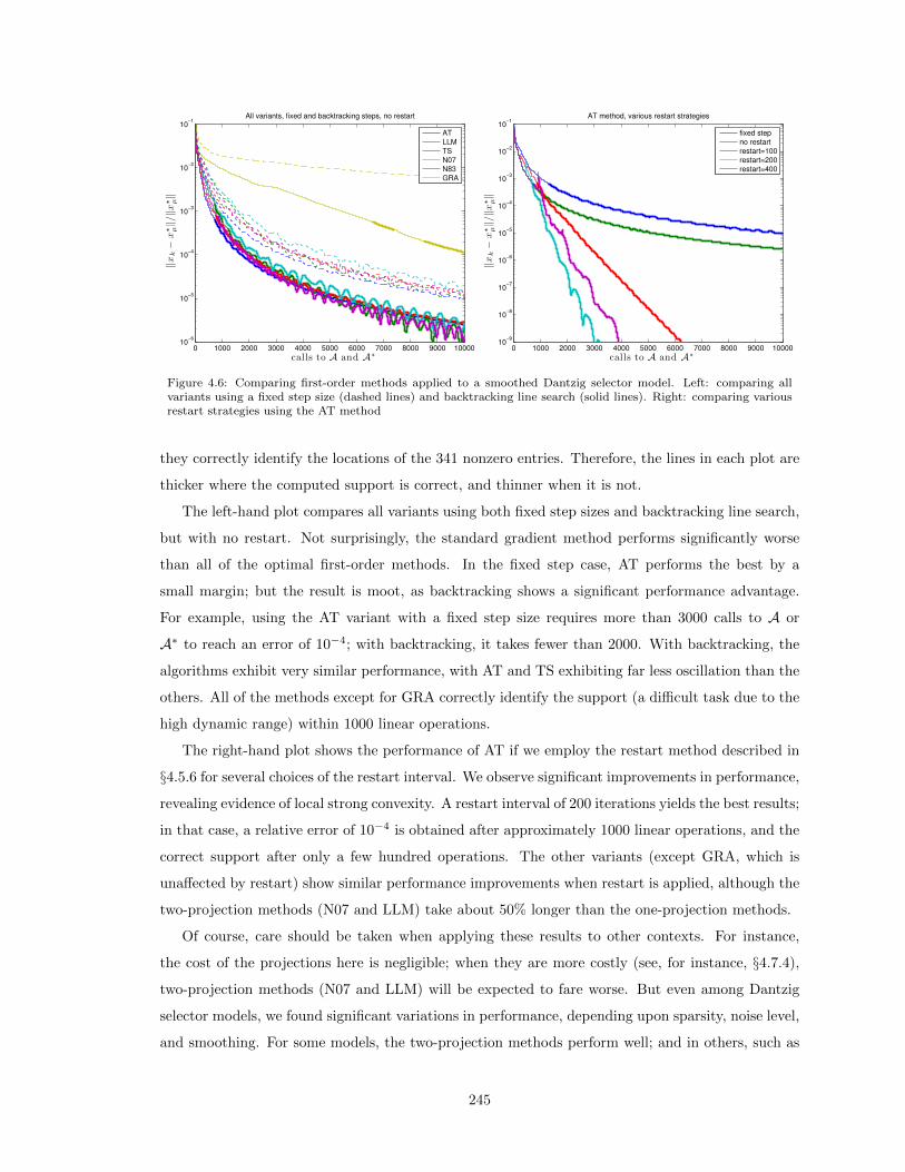
0 1000 2000 3000 4000 5000 6000 7000 8000 9000 1000010

−6

10−5

10−4

10−3

10−2

10−1

calls to A and A∗

‖xk−

x⋆ µ‖/

‖x⋆ µ‖

All variants, fixed and backtracking steps, no restart

AT

LLM

TS

N07

N83

GRA

0 1000 2000 3000 4000 5000 6000 7000 8000 9000 1000010

−9

10−8

10−7

10−6

10−5

10−4

10−3

10−2

10−1

calls to A and A∗

‖xk−

x⋆ µ‖/

‖x⋆ µ‖

AT method, various restart strategies

fixed step

no restart

restart=100

restart=200

restart=400

Figure 4.6: Comparing first-order methods applied to a smoothed Dantzig selector model. Left: comparing allvariants using a fixed step size (dashed lines) and backtracking line search (solid lines). Right: comparing variousrestart strategies using the AT method

they correctly identify the locations of the 341 nonzero entries. Therefore, the lines in each plot are

thicker where the computed support is correct, and thinner when it is not.

The left-hand plot compares all variants using both fixed step sizes and backtracking line search,

but with no restart. Not surprisingly, the standard gradient method performs significantly worse

than all of the optimal first-order methods. In the fixed step case, AT performs the best by a

small margin; but the result is moot, as backtracking shows a significant performance advantage.

For example, using the AT variant with a fixed step size requires more than 3000 calls to A or

A∗ to reach an error of 10−4; with backtracking, it takes fewer than 2000. With backtracking, the

algorithms exhibit very similar performance, with AT and TS exhibiting far less oscillation than the

others. All of the methods except for GRA correctly identify the support (a difficult task due to the

high dynamic range) within 1000 linear operations.

The right-hand plot shows the performance of AT if we employ the restart method described in

§4.5.6 for several choices of the restart interval. We observe significant improvements in performance,

revealing evidence of local strong convexity. A restart interval of 200 iterations yields the best results;

in that case, a relative error of 10−4 is obtained after approximately 1000 linear operations, and the

correct support after only a few hundred operations. The other variants (except GRA, which is

unaffected by restart) show similar performance improvements when restart is applied, although the

two-projection methods (N07 and LLM) take about 50% longer than the one-projection methods.

Of course, care should be taken when applying these results to other contexts. For instance,

the cost of the projections here is negligible; when they are more costly (see, for instance, §4.7.4),

two-projection methods (N07 and LLM) will be expected to fare worse. But even among Dantzig

selector models, we found significant variations in performance, depending upon sparsity, noise level,

and smoothing. For some models, the two-projection methods perform well; and in others, such as

245

0 100 200 300 400 500 600 700 800 90010

−14

10−12

10−10

10−8

10−6

10−4

10−2

100

number of calls to A and A∗

rela

tive

erro

r

AT w/o continuationAT w/ accel. continuationSPGL1

0 200 400 600 800 1000 1200 1400 1600 1800 2000

10−10

10−8

10−6

10−4

10−2

100

number of calls to A and A∗

rela

tive

erro

r

AT w/o continuationAT w/ continuationSPGL1

Figure 4.7: Comparisons of the dual solver with SPGL1. The plot on the left involves a noiseless basis pursuitmodel, while the plot on the right represents a noisy image model.

when we have local strong convexity, gradient descent performs well (when compared to the other

algorithms without restart). Overall, it seems there is no best algorithm, but we choose the AT

algorithm as our default, since in our experience it is consistently one of the best and only requires

one projection per iteration.

4.7.2 LASSO: comparison with SPGL1

As mentioned in the introduction, there are numerous algorithms for solving the LASSO. Yet the

algorithm produced by our dual conic approach is novel; and despite its apparent simplicity, it is

competitive with the state of the art. To show this, we compared the AT first-order variant with

SPGL1 [vdBF08], chosen because recent and extensive tests in [BBC11] suggest that it is one of the

best available methods.

The nature of the SPGL1 algorithm, which solves a sequence of related problems in a root-

finding-scheme, is such that it is fastest when the noise parameter ε is large, and slowest when ε = 0.

To compare performance in both regimes, we constructed two tests. The first is an “academic”

test with an s-sparse signal and no noise; however, we choose s large enough so that the LASSO

solution does not coincide with the sparse solution, since empirically this is more challenging for

solvers. Specifically, the measurement matrix A is a 213 × 214 partial DCT, while the optimal value

x? was constructed to have s = 212 nonzeros. The second test uses Haar wavelet coefficients from

the “cameraman” test image (Figure 4.8 (a)) which decay roughly according to a power law, and

adds noise with a signal-to-noise ratio of 30 dB. The measurement matrix is also a partial DCT, this

time of size 0.3 · 216 × 216.

Figure 4.7 shows the results from both tests, each plot depicting relative error ‖xk − x?‖/‖x?‖versus the number of linear operations. We see that both methods achieve several digits of accuracy

246

in just a few hundred applications of A and its adjoint. SPGL1 outperforms a regular AT solver

in the left-hand “academic” test; however, AT with accelerated continuation solves the problem

significantly faster than SPGL1. The noiseless case exploits our method’s strength since the exact

penalty property holds.

For the wavelet test, SPGL1 outperforms our method, even when we use continuation. Although

AT with continuation achieves high levels of accuracy in fewer than 1000 operations, other tests

confirmed that SPGL1 is often a little better than our method, especially for large ε. But the dual

conic approach is competitive in many cases, and can be applied to a wider class of problems9.

4.7.3 Wavelet analysis with total-variation

The benefit of our approach is highlighted by the fact that we can solve complicated composite

objective functions. Using the solver templates, it is easy to solve the `1-analysis and TV problem

from §4.4.6. We consider here a denoising problem with full observations; i.e., A = I. Figure 4.8 (a)

shows the original image x0, to which noise is added to give an image y = x0 + z with a signal-to-

noise ratio of 20 dB (see subplot (b)). In the figure, error is measured in peak-signal-to-noise ratio

(PSNR), which for an n1 × n2 image x with pixel values between in [0, 1] is defined as

PSNR(x) = 20 log10

( √n1n2

‖x− x0‖F

)

where x0 is the noiseless image.

To denoise, we work with a 9/7 bi-orthogonal wavelet transformW (similar to that in JPEG-2000)

with periodic boundary conditions (the periodicity is not ideal to achieve the lowest distortion). A

simple denoising approach is to hard-threshold the wavelet coefficientsWx and then invert withW−1.

Figure 4.8 (c) shows the result, where the hard-threshold parameter was determined experimentally

to give the best PSNR. We refer to this as “oracle thresholding” since we used the knowledge of x0

to determine the threshold parameter. As is common with wavelet methods [SNM03], edges in the

figure induce artifacts.

Figures 4.8 (d), (e), and (f) are produced using the solvers in this chapter, solving

minimize α‖Wx‖1 + β‖x‖TV + µ2 ‖x− y‖2F

subject to ‖Ax− y‖2 ≤ ε.(4.7.1)

Figure 4.8 (d) employs wavelet analysis only (α = 1, β = 0), (e) just TV (α = 0, β = 1), and (f) both

(α = 1, β = 5). For the best performance, the matrix A was re-scaled so that all the dual variables

are of the same order; see [BCG10b] for further discussion of scaling.

9SPGL1 is also flexible in the choice of norm, but notably, it cannot solve the analysis problem due to difficultiesin the primal projection.

247

(a) Original (b) Noisy version (25.6 dB PSNR)

(c) Wavelet thresholded (28.3 dB PSNR) (d) Wavelet `1-analysis (29.0 dB PSNR)

(e) TV minimization (30.9 dB PSNR) (f) Wavelet analysis + TV minimization (31.0 dB PSNR)Figure 4.8: Denoising an n = 2562 image

248

The Frobenius term in (4.7.1) is of course for smoothing purposes, and it is possible to minimize

its effect by choosing µ small or using the continuation techniques discussed. But for denoising, its

presence makes little difference; in fact, it may give more visually pleasing results to use a relatively

large µ. So to determine µ, we started with an estimate like

µ = max(α‖Wy‖1, β‖y‖TV )/c

with c ' 500 and then adjusted to give reasonable results. We ultimately employed µ = 1 for (d),

µ = 50 for (e), and µ = 160 for (f).

The wavelet analysis run took 26 iterations, and was complete in about 5 seconds. As shown in

image (d), it produced boundary effects that are noticeable to the eye, and similar to those produced

by thresholded image (c). The TV model (e) and TV with wavelets model (f) took 37 iterations (3

seconds) and 30 iterations (8 seconds), respectively. Both produced better reconstructions, both by

PSNR and by visual inspection. The additional wavelet analysis term in plot (f) offers only minimal

improvement over TV alone, but this may be due to our simple choice of wavelet transform. For

example, undecimated wavelets are common in denoising and may give better results, but our point

here is simplicity and to point out the flexibility of the framework.

4.7.4 Matrix completion: expensive projections

We consider the nuclear-norm minimization problem (4.4.2) of a matrix X ∈ Rn1×n2 in the conic

dual smoothing approach. For matrix completion, the linear operator A is the subsampling operator

revealing entries in some subset E ⊂ [n1] × [n2]. With equality constraints (ε = 0) and X0 = 0,

gradient ascent on the dual is equivalent to the SVT algorithm of [CCS10], a reference which also

considered non-equality constraints, e.g., of the form (4.4.2).

In addition to our own interest in this problem, one of the reasons we chose it for this article

is that it differs from the others in one key respect: its computational cost is dominated by one of

the projections, not by the linear operators. After all, the linear operator in this case is no more

than a set of memory accesses, while the primal projection requires the computation of at least the

largest singular values of a large matrix. As a result, the considerations we bring to the design of

an efficient solver are unique in comparison to the other examples presented.

There are a number of strategies we can employ to reduce the cost of this computation. The key

is to exploit the fact that a nuclear-norm matrix completion model is primarily of interest when its

optimal value X? is expected to have low rank [CR09]. Recall from §4.4.3 that the update of Xk

takes the form

Xk = SoftThresholdSingVal(X0 − µ−1A∗(λ), µ−1

).

249

0 200 400 600 800 1000 120010

−14

10−12

10−10

10−8

10−6

10−4

10−2

100

calls to SoftThresholdSingVal

erro

r

GRA, backtrackingAT, backtrackingAT, restart every 10AT, restart every 50AT, restart every 100

Figure 4.9: Noiseless matrix completion using various first-order methods

Our numerical experiments show that if µ is sufficiently small, the ranks rk = rank(Xk) will remain

within the neighborhood of r? = rank(X?). In fact, with µ sufficiently small and X0 = 0, the rank

grows monotonically.

There are a variety of ways we can exploit the low-rank structure of the iterates Xk. By storing

Xk = UkΣkVk in factored form, we can reduce the storage costs from O(n1n2) to O(rk(n1 + n2)).

The quantity A(Xk), used in the computation of the gradient of the dual function, can be computed

efficiently from this factored form as well. Finally, using a Lanczos method such as PROPACK

[Lar04], the cost of computing the necessary singular values will be roughly proportional to rk.

By combining these techniques, the overall result is that the cost of singular value thresholding is

roughly linear in the rank of its result. These techniques are discussed in more detail in [BCG10b].

Smaller values of µ, therefore, reduce the ranks of the iterates Xk, thereby reducing the com-

putational cost of each iteration. This leads to a unique trade off, however: as we already know,

smaller values of µ increase the number of iterations required for convergence. In practice, we have

found that it is indeed best to choose a small value of µ, and not to employ continuation.

For our numerical example, we constructed a rank-10 matrix of size n1 = n2 = 1000, and

randomly selected 10% of the entries for measurement—about 5 times the number of degrees of

freedom in the original matrix. We solved this problem using three variations of GRA and five

variations of AT, varying the step size choices and the restart parameter. The smoothing parameter

was chosen to be µ = 10−4, for which all of the methods yield a monotonic increase in the rank

of the primal variable. The pure gradient method took about 1.8 minutes to reach 10−4 relative

error, while the AT method without restart took twice the time; the error is in the Frobenius norm,

comparing against the true low-rank matrix, which is the solution to the unperturbed problem.

250

The results of our experiments are summarized in Figure 4.9. The horizontal axis now gives the

number of SoftThresholdSingVal operations, a more accurate measure of the cost in this case; the

cost of a SoftThresholdSingVal call is not fixed, but we observe that the rank of the iterates quickly

reaches 10 and most SoftThresholdSingVal calls have roughly the same cost. The salient feature of

this figure is that while AT initially outperforms GRA, the linear convergence exhibited by GRA

allows it to overtake AT at moderate levels of precision. Employing a restart method with AT

improves its performance significantly; and for a restart intervals of 50 iterations, its performance

approaches that of GRA, but it does not overtake it.

What accounts for this performance reversal? First, we observe that AT requires two projections

per iteration while GRA requires only one. This difference is inconsequential in our other examples,

but not for this one; and it is due to our use of the backtracking line search. Switching to a fixed

step size eliminated the extra projection, but the overall performance suffered significantly. We hope

to identify a new line search approach that avoids the added cost revealed here.

Second, the similarities of Figures 4.5 and 4.9 suggest the presence of strong convexity. Using

an estimate of the decay rate for gradient descent with step size t = 1/Lf , and comparing with

known decay rate estimates [Nes04] gives an estimate of mf = 0.0024. For this value of mf (and

with Lf = 1), the optimal restart number Kopt from [GLW09] is about 80, which is consistent with

the plot. It is easy to verify, however, that the smoothed dual function is not strongly convex.

The results suggest, then, that local strong convexity is present. The authors in [GLW09] argue

that for compressed sensing problems whose measurement matrices satisfy the restricted isometry

property, the primal objective is locally strongly convex when the primal variable is sufficiently

sparse. The same reasoning may apply to the matrix completion problem; the operator A∗A is

nearly isometric (up to a scaling) when restricted to the set of low-rank matrices. The effect may be

amplified by the fact that we have taken pains to ensure that the iterates remain low-rank. Overall,

this effect is not yet well understood, but will also be explored in later work.

We note that if the underlying matrix is not low-rank, then the local strong convexity effect is not

present, and gradient descent does not outperform the AT method. In this case, our experiments

also suggest that the restart method has little effect. Likewise, when inequality constraints are

added we observe that the unusually good performance of gradient descent vanishes. For both the

non-low-rank and noisy cases, then, it may be beneficial to employ an optimal first-order method

and to use continuation.

Figure 4.10 demonstrates these claims on a noisy matrix completion problem. We constructed

a 50 × 45 matrix of rank 20, sampled 67% of the entries, and added white noise to yield a 30 dB

SNR. By using this small problem size, we are able to use CVX [GB10] to compute a reference

solution; this took 5.4 minutes. The figure depicts three different approaches to solving the problem:

GRA and AT each with µ = 5 · 10−4 and no continuation; and AT with µ = 10−2 and accelerated

251

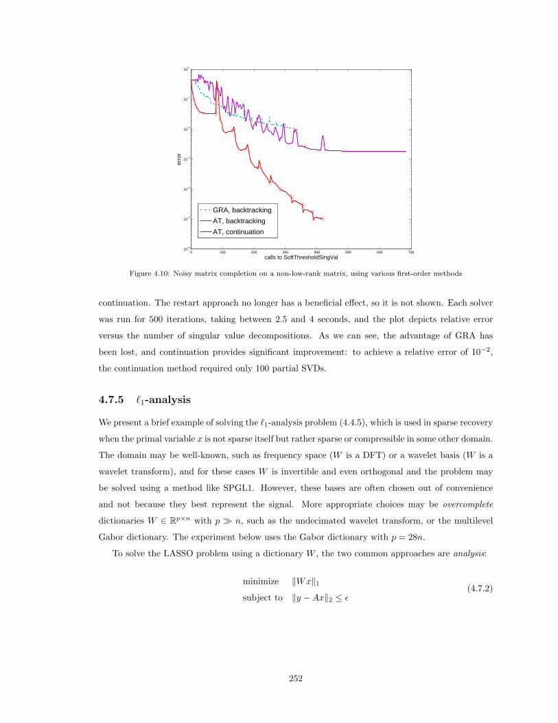
0 100 200 300 400 500 600 70010

−6

10−5

10−4

10−3

10−2

10−1

100

calls to SoftThresholdSingVal

erro

r

GRA, backtracking

AT, backtracking

AT, continuation

Figure 4.10: Noisy matrix completion on a non-low-rank matrix, using various first-order methods

continuation. The restart approach no longer has a beneficial effect, so it is not shown. Each solver

was run for 500 iterations, taking between 2.5 and 4 seconds, and the plot depicts relative error

versus the number of singular value decompositions. As we can see, the advantage of GRA has

been lost, and continuation provides significant improvement: to achieve a relative error of 10−2,

the continuation method required only 100 partial SVDs.

4.7.5 `1-analysis

We present a brief example of solving the `1-analysis problem (4.4.5), which is used in sparse recovery

when the primal variable x is not sparse itself but rather sparse or compressible in some other domain.

The domain may be well-known, such as frequency space (W is a DFT) or a wavelet basis (W is a

wavelet transform), and for these cases W is invertible and even orthogonal and the problem may

be solved using a method like SPGL1. However, these bases are often chosen out of convenience

and not because they best represent the signal. More appropriate choices may be overcomplete

dictionaries W ∈ Rp×n with p � n, such as the undecimated wavelet transform, or the multilevel

Gabor dictionary. The experiment below uses the Gabor dictionary with p = 28n.

To solve the LASSO problem using a dictionary W , the two common approaches are analysis:

minimize ‖Wx‖1subject to ‖y −Ax‖2 ≤ ε

(4.7.2)

252

and synthesis:

minimize ‖α‖1subject to ‖y −AW ∗α‖2 ≤ ε,

(4.7.3)

with decision variable α. Similarly, the Dantzig selector approach would have the same objectives

but constraints of the form ‖A∗(y −Ax)‖∞ ≤ δ (analysis) and ‖A∗(y −AW ∗α)‖∞ ≤ δ (synthesis).

When W is not orthogonal, the two approaches are generally different in non-trivial ways, and

furthermore, the solutions to synthesis may be overly sensitive to the data [EMR07].

The differences between analysis and synthesis are not very well understood at the moment for

two reasons. The first is that the analysis problem has not been studied theoretically. An exception

is the very recent paper [CENR11] which provides the first results for `1-analysis. The second is that

there are no existing efficient first-order algorithms to solve the analysis problem, with the exception

of the recent NESTA [BBC11] and C-SALSA [ABDF11] algorithms, which both work on the LASSO

version, and only when AA∗ = I.

With the dual conic approach, it is now possible to solve the smoothed analysis problem, and by

using continuation techniques, the effect of the smoothing is negligible. To illustrate, we constructed

a realistic test of the recovery of two radio-frequency radar pulses that overlap in time, as depicted

in Figure 4.11. The first pulse is large, while the second pulse has 60 dB smaller amplitude. Both

have carrier frequencies and phases that are chosen uniformly at random, and noise is added so that

the small pulse has a signal-to-noise ratio of 0.1 dB.

The signal is recovered at Nyquist rate resolution for 2.5 GHz bandwidth, and the time period

is a little over 1600 ns, so that n = 8,192. The sensing matrix A is modeled as a block-diagonal

matrix with ±1 entries on the blocks, representing a system that randomly mixes and integrates the

input signal, taking 8 measurements every 100 ns, which is 12.5× below the Nyquist rate. Thus A

is a 648 × 8,192 matrix and W is a 228,864 × 8,192 matrix. We applied both the Dantzig selector

and LASSO models to this problem.

To solve the problems, we employed the AT variant with accelerated continuation. At each

iteration, the stopping tolerance is decreased by a factor of 1.5, and the continuation loop is ended

when it no longer produces significantly different answers, which is usually between 2 and 8 iterations.

The value of µ is set to

µ = 0.1‖WxLS‖212‖xLS‖2

, (4.7.4)

where xLS is the least-squares solution to Ax = y, which is easy to calculate since m � n (and

independent of p).

To enhance the results, we employed an outer reweighting loop [CWB08], in which we replace

the ‖Wx‖1 term with ‖RWx‖1 for some diagonal weight matrix R. Each reweighting involves a

full solve of either the Dantzig selector or the LASSO. This loop is run until convergence, which is

253

0 0.5 1 1.5 2 2.5−220

−200

−180

−160

−140

−120

−100

−80

−60

Frequency (GHz)

Pow

er/fr

eque

ncy

(dB

/Hz)

Original signalRecovered signal

0 0.5 1 1.5 2 2.5−220

−200

−180

−160

−140

−120

−100

−80

−60

Frequency (GHz)

Pow

er/fr

eque

ncy

(dB

/Hz)

Original signalRecovered signal

Figure 4.11: Recovery of a small pulse 60 dB below a large pulse. The first plot employs a Dantzig selector, thebottom employs LASSO.

254

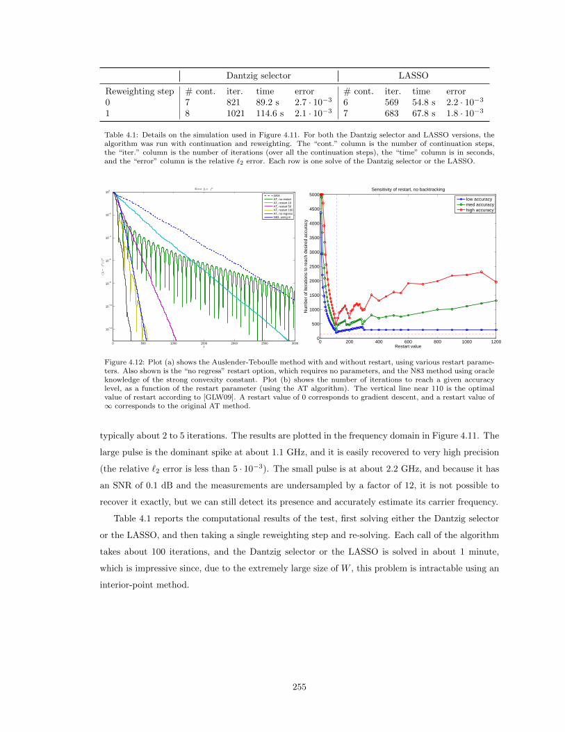
Dantzig selector LASSO

Reweighting step # cont. iter. time error # cont. iter. time error0 7 821 89.2 s 2.7 · 10−3 6 569 54.8 s 2.2 · 10−3

1 8 1021 114.6 s 2.1 · 10−3 7 683 67.8 s 1.8 · 10−3

Table 4.1: Details on the simulation used in Figure 4.11. For both the Dantzig selector and LASSO versions, thealgorithm was run with continuation and reweighting. The “cont.” column is the number of continuation steps,the “iter.” column is the number of iterations (over all the continuation steps), the “time” column is in seconds,and the “error” column is the relative `2 error. Each row is one solve of the Dantzig selector or the LASSO.

0 500 1000 1500 2000 2500 3000

10−12

10−10

10−8

10−6

10−4

10−2

100

k

(fk−−

f?)/

f?

Error fk−− f?

GRAAT, no restartAT, restart 10AT, restart 50AT, restart 100AT, no regressN83, using m

0 200 400 600 800 1000 12000

500

1000

1500

2000

2500

3000

3500

4000

4500

5000

Restart value

Num

ber

of it

erat

ions

to r

each

des

ired

accu

racy

Sensitivity of restart, no backtracking

low accuracymed accuracyhigh accuracy

Figure 4.12: Plot (a) shows the Auslender-Teboulle method with and without restart, using various restart parame-ters. Also shown is the “no regress” restart option, which requires no parameters, and the N83 method using oracleknowledge of the strong convexity constant. Plot (b) shows the number of iterations to reach a given accuracylevel, as a function of the restart parameter (using the AT algorithm). The vertical line near 110 is the optimalvalue of restart according to [GLW09]. A restart value of 0 corresponds to gradient descent, and a restart value of∞ corresponds to the original AT method.

typically about 2 to 5 iterations. The results are plotted in the frequency domain in Figure 4.11. The

large pulse is the dominant spike at about 1.1 GHz, and it is easily recovered to very high precision

(the relative `2 error is less than 5 · 10−3). The small pulse is at about 2.2 GHz, and because it has

an SNR of 0.1 dB and the measurements are undersampled by a factor of 12, it is not possible to

recover it exactly, but we can still detect its presence and accurately estimate its carrier frequency.

Table 4.1 reports the computational results of the test, first solving either the Dantzig selector

or the LASSO, and then taking a single reweighting step and re-solving. Each call of the algorithm

takes about 100 iterations, and the Dantzig selector or the LASSO is solved in about 1 minute,

which is impressive since, due to the extremely large size of W , this problem is intractable using an

interior-point method.

255

4.8 Extensions

4.8.1 Automatic restart

When a function is strongly convex, gradient descent converges linearly. If the strong convexity

constant mf is known, then accelerated methods such as N83 also converge linearly, and with a

better rate than for gradient descent. However, if mf is unknown, the accelerated methods do not

converge linearly. This is shown in Figure 4.12(a). Our proposed solution from §4.5.6 is to restart

the method every R iterations, which then guarantees linear convergence [Nes07]. The optimal rate

of convergence is obtained when R = R(mf ), which is unknown a priori, so R must be estimated.

Figure 4.12(b) shows that as long as R > R(mf ) (R(mf ) is shown as the vertical line), then the

method still converges quickly, and hence R is not an extremely sensitive parameter.

However, R may not be scale-invariant, and estimating R is still an issue. One solution is

an automatic restart, which requires no parameter. Whenever the objective shows non-monotonic

behavior, a restart is forced. Figure 4.12(a) shows this method, called “no regress”, compared

to the N83 method using “oracle” knowledge of mf . The automatic method performs extremely

well. We note that many restart ideas have been explored in the non-linear conjugate-gradient (CG)

literature since the late 1970s [Pow77]. The prevailing intuition for CG, according to [NW06], is that

restart should be performed once the iterate is in an approximately quadratic region surrounding

the minimum, since then the non-linear CG will perform similarly to linear CG, assuming the line

search is good, and convergence will be rapid.

4.8.2 Specialized solvers for certain problems

We consider some specific optimization problems for which there is special structure to exploit. One

of the advantages of TFOCS is that the solver is a module that can be swapped, so it is easy to

implement specialized algorithms.

4.8.2.1 Noiseless basis pursuit

The noiseless basis pursuit problem,

minx‖x‖1 such that Ax = b

has an unconstrained differentiable dual after smoothing is applied; it is also a linear program, so

it enjoys the exact-penalty property. Because the dual is unconstrained, it is easy to use a solver

like SESOP [EMZ07], BFGS or L-BFGS [BLN95], or a non-linear conjugate-gradient algorithm.

Figure 4.13 shows an experiment on a basis pursuit problem with N = 2048 variables and a partial

DCT measurement matrix A with 1024 rows. The original signal has 146 nonzeros. We compare

256

0 200 400 600 800 1000 1200 1400 1600 1800 200010

−14

10−12

10−10

10−8

10−6

10−4

10−2

100

102

number of calls to A and A∗

‖xk−–

x?‖

tfocs (GRA)tfocs (AT)tfocs w/ restarttfocs with CG

Figure 4.13: Noiseless basis pursuit, comparing a non-linear CG method to an optimal first-order method.

gradient descent, Auslender-Teboulle’s (AT) algorithm, the AT algorithm with restart, and a modern

non-linear CG method called CG-851 [HZ06]. All of the AT methods are efficient, but the non-linear

CG method is even faster. This shows the flexibility of TFOCS and suggests that the long history of

work put into CG methods may be applicable to a few special inverse problems. The main difficulty

with CG is that standard CG algorithms do not handle constraints, and that the algorithms need

appropriate line search. The performance of CG is extremely sensitive to the type of line search;

we thank Michael McCoy for providing the line search code used in this experiment. It may also be

possible to use specific exact line search algorithms; for example, it is easy to derive an exact line

search when the objective contains a `1 norm and a quadratic term (see, e.g., [WYGZ10]).

We also note recent work on the performance of BFGS on non-smooth problems [LO09,YVGS10]

(that is, when the objective is differentiable but not second-order differentiable). This is the case

for noiseless basis pursuit (and also for noiseless matrix completion with the nuclear norm).

4.8.2.2 Conic problems in standard form

Consider the conic problem

minimizex

〈c, x〉 such that x ≥K 0, Ax = b (4.8.1)

where x ≥K 0 means x ∈ K. If K = Rn+, then this reduces to x ≥ 0 component-wise, and the problem

is a linear program (LP). If K is the Lorentz cone, then the problem is a second-order cone program

(SOCP). If K is the positive semi-definite cone, in which case x and c are Hermitian matrices and

the inner product 〈c, x〉 = trace cx is the inner product which induces the Hilbert-Schmidt norm,

and then the problem is a semi-definite program (SDP).

257

0 500 1000 1500 2000 2500 300010

−2

10−1

100

101

102

iterations

rela

tive

err

or

AT with restart and continuationL-BFGS-B with continuation

Figure 4.14: Comparison of AT method and L-BFGS-B on a standard form linear program. Both methods behavesimilarly.

The dual problem is

maxν,λ−〈b, ν〉 such that λ ≥K 0, λ = c+A∗ν

which may not be easier to solve than the primal. It is possible to eliminate the variable λ, but we

prefer to keep it since it makes it clear that there is a coupling between the inequality and equality

constraints.

To apply the dual formulation, we smooth the objective by adding a term µ2 ‖x−x0‖2 where ‖ · ‖

is the norm induced by the appropriate inner-product. This has the effect of uncoupling the dual

variables. The dual problem is now

maxν,λ−〈b, ν〉 − 1

2µ‖c− λ+A∗ν‖2 + 〈c− λ+A∗ν, x0〉 such that λ ≥K 0.

The dual is quadratic with no equality constraints and a simple inequality constraint. For K =

Rn+, this is part of a box-constraint, and many algorithms take advantage of its simplicity. Figure 4.14

shows a comparison between TFOCS using the AT method (with restart and continuation) and the

L-BFGS-B method [BLN95,ZBLN97]. L-BFGS-B is a box constrained version of the limited memory

BFGS quasi-Newton method. The BFGS method is well-regarded as one of the fastest methods,

when it is applicable. In the figure, we see that L-BFGS-B performs about the same as the optimal

method, which is slightly discouraging. There may be tweaks or special considerations which can

make L-BFGS-B achieve the same performance as BFGS.

The technique of adding a quadratic term to a linear program has been used since at least

Mangasarian in the early 1980s [Man81].

258

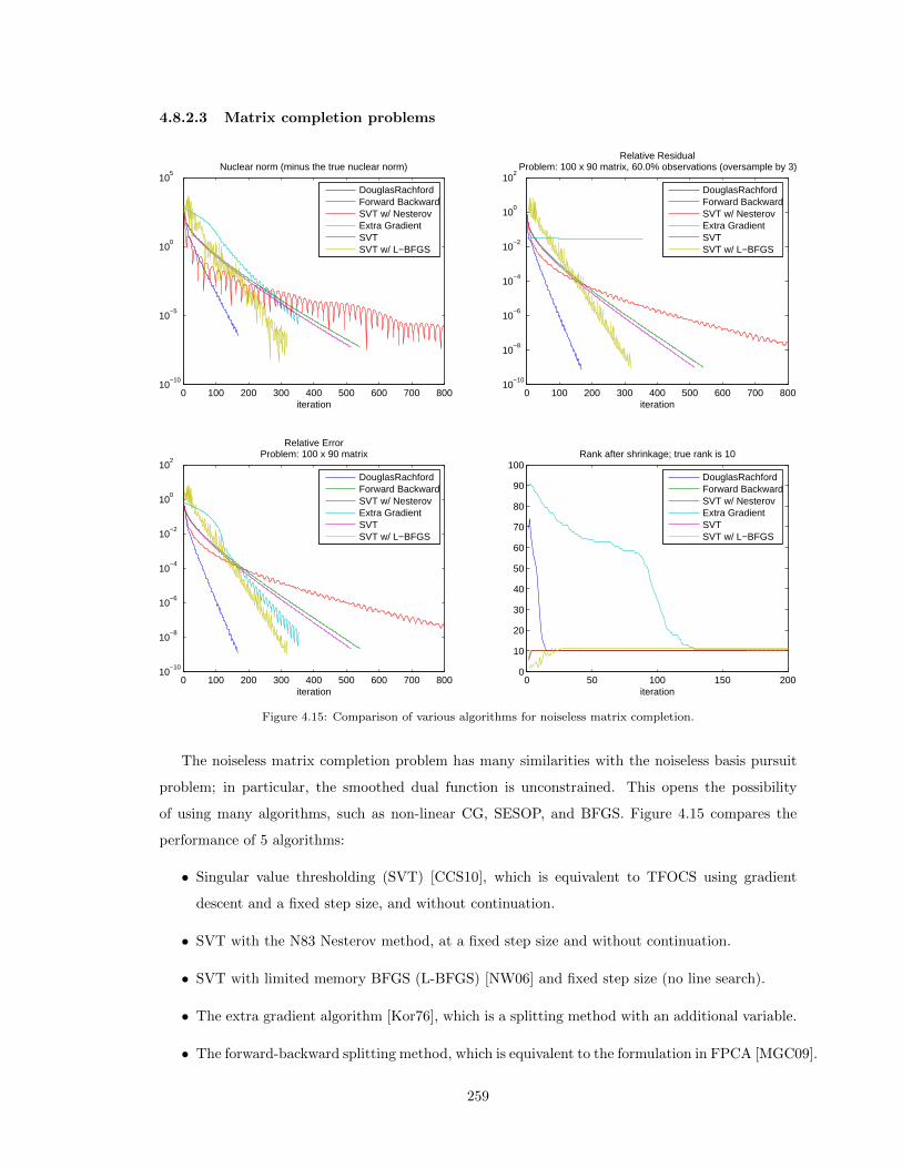
4.8.2.3 Matrix completion problems

0 100 200 300 400 500 600 700 80010

−10

10−5

100

105

Nuclear norm (minus the true nuclear norm)

iteration

DouglasRachfordForward BackwardSVT w/ NesterovExtra GradientSVTSVT w/ L−BFGS

0 100 200 300 400 500 600 700 80010

−10

10−8

10−6

10−4

10−2

100

102

Relative ResidualProblem: 100 x 90 matrix, 60.0% observations (oversample by 3)

iteration

DouglasRachfordForward BackwardSVT w/ NesterovExtra GradientSVTSVT w/ L−BFGS

0 100 200 300 400 500 600 700 80010

−10

10−8

10−6

10−4

10−2

100

102

Relative ErrorProblem: 100 x 90 matrix

iteration

DouglasRachfordForward BackwardSVT w/ NesterovExtra GradientSVTSVT w/ L−BFGS

0 50 100 150 2000

10

20

30

40

50

60

70

80

90

100Rank after shrinkage; true rank is 10

iteration

DouglasRachfordForward BackwardSVT w/ NesterovExtra GradientSVTSVT w/ L−BFGS

Figure 4.15: Comparison of various algorithms for noiseless matrix completion.

The noiseless matrix completion problem has many similarities with the noiseless basis pursuit

problem; in particular, the smoothed dual function is unconstrained. This opens the possibility

of using many algorithms, such as non-linear CG, SESOP, and BFGS. Figure 4.15 compares the

performance of 5 algorithms:

• Singular value thresholding (SVT) [CCS10], which is equivalent to TFOCS using gradient

descent and a fixed step size, and without continuation.

• SVT with the N83 Nesterov method, at a fixed step size and without continuation.

• SVT with limited memory BFGS (L-BFGS) [NW06] and fixed step size (no line search).

• The extra gradient algorithm [Kor76], which is a splitting method with an additional variable.

• The forward-backward splitting method, which is equivalent to the formulation in FPCA [MGC09].

259

• The Douglas-Rachford splitting method [Com04].

To be fair, the comparisons use fixed-step sizes for all algorithms; of course, most of the algorithms

benefit enormously from using line search, as we have shown in this chapter, so these results are not

necessarily “real-world” results.

The special consideration in the matrix completion problem is that the matrix shrinkage step

is expensive to compute; see the discussion in §4.7.4. One method, used in [MGC09], is to use

randomized linear algebra to compute an approximate SVD. Another method is using a Lanczos-

based method such as PROPACK [Lar04]. For a Lanczos-based method, only singular values above

a threshold size are needed; the number of iterations in the SVD computation is directly proportional

to the number of singular values above this threshold. Furthermore, the cost of each matrix-vector

multiply depends on the rank of the previous iterate, since the current iterate is a combination of a

sparse and low-rank matrix.

Figure 4.15 shows results using a dense SVD factorization, but also records the rank. All the

algorithms converge quickly, but Douglas-Rachford and SVT-with-L-BFGS are considerably faster

than the rest. The lower-right plot shows the ranks of the variables at every iteration. The benefit

of SVT-based methods is that the rank typically starts at 0 and increases slowly to a steady-state

value (this need not be true with line search variants). The Douglas-Rachford algorithm, on the

other hand, takes a very aggressive first few steps and the rank is very high, before coming lower. On

a large-scale problem, this means the first few iterations might be too expensive to even compute.

The extra-gradient method has even slower decay toward the true rank.

Despite the issues with rank, the Douglas-Rachford method is promising due to the rapid con-

vergence, so it may be possible to adjust it to keep the ranks smaller. Thanks to Jalal Fadili for

ideas and code regarding these splitting methods.

With matrix completion problems, there is tremendous room for improvement, since high-

accuracy SVDs are unnecessary in the initial steps of the algorithm. There has been some reported

success of using methods from [HMT11] with the matrix completion problem because these types of

approximate SVDs can take advantage of warm-starts. Another recent paper mentions improvements

using warm-started Lanczos methods [LW10].

4.9 Software: TFOCS

The work described in this paper has been incorporated into a software package, Templates for First-

Order Conic Solvers (TFOCS, pronounced tee-fox ), which is publicly available at http://tfocs.

stanford.edu. As its name implies, this package is a set of templates, or building blocks, that can

be used to construct efficient, customized solvers for a variety of models.

To illustrate the usage of the software, let us show how to construct a simple solver for the

260

smoothed Dantzig selector model described in §4.3. We will begin by assuming that we are given

the problem data A, b, delta, and a fixed smoothing parameter mu. The basic solver templates

require two functions to complete their work. The first function computes the value and gradient of

gsmooth, the smooth component of the composite dual:

function [ val, grad, x ] = g_dantzig( A, y, x0, mu, z )

x = SoftThreshold( x0 - (1/mu) * A’ * ( A * z ), 1/mu );

grad = A’ * ( y - A * x );

val = z’ * grad - norm( x, 1 ) - 0.5 * mu * norm( x - x0 ) .^ 2;

The second function computes the generalized projection associated with the nonsmooth component

of the dual, which is in this case h(z) = δ‖z‖1.

h = prox_scale( tfocs_prox( @(z)norm(z,1), @SoftThreshold ), delta );

The tfocs prox function combines h and the proximity operator of h in a fashion that the software

understands, and prox scale adjusts h from ‖z‖1 to δ‖z‖1 and also updates the proximity operator.

The functions h and g depend on the soft-thresholding operator:

function y = SoftThreshold( x, t )

y = sign( x ) .* max( abs( x ) - t, 0 );

Armed with these functions, the following code solves the smoothed Dantzig selector, using the

Auslender/Teboulle first-order variant and the default choices for line search and stopping criteria.

function x = Dantzig_smoothed( A, y, delta, mu )

[m,n] = size(A);

x0 = zeros(n,1); z0 = zeros(n,1);

g_sm = @(z) g_dantzig( A, y, x0, mu, z );

affine = [];

z = tfocs_AT( g_sm_op, affine, h, z0 );

x = SoftThreshold( x0 - (1/mu) * A’ * ( A * z ), 1/mu );

The second-to-last line of code calls the AT solver.

This simple solver is likely to be unnecessarily inefficient if A exhibits any sort of fast operator

structure, but this can be remedied rather simply. Note that the solver itself needs to have no knowl-

edge of A or y above; its interaction with these quantities comes only through calls to g_dantzig.

Therefore, we are free to rewrite g_dantzig in a more numerically efficient manner: for instance,

if A is derived from a Fourier transform, we may substitute fast Fourier transform operations for

matrix-vector multiplications. This simple change will reduce the cost of each iteration from O(mn)

261

to O(n log n), and the storage requirements from O(n2) to O(n). For large-scale problems these

savings can be quite significant.

A further improvement in performance is possible through careful management of the linear

operator calculations as described in §4.5.4. The TFOCS solver templates can perform this manage-

ment automatically. To take advantage of it, we replace g_dantzig with two functions: one which

implements the underlying linear operator, and one which implements the remainder of the smooth

function. The details of how to accomplish this are best left to the user guide [BCG10b].

Of course, as part of the complete package, we have supplied a solver for the Dantzig selector

that exploits each of these efficiencies, and others. Similar solvers have been created for the LASSO,

TV, and other models discussed here. But the flexibility of the lower-level templates will allow

these same efficiencies to be achieved for many models that we have not discussed here. In fact,

evidently the templates are not restricted to our specific conic form (4.1.9) or its dual, and we hope

the software finds application outside of the compressed sensing domain as well.

With the software release is a detailed user guide [BCG10b] that covers the usage, documents

the most popular problem formulations, and provides some examples. We refer the reader to the

user guide for further software details.

4.10 Discussion

We have developed a convenient framework for constructing first-order methods, which is flexible and

handles a variety of convex cone problems, including problems that did not have efficient algorithms

before. On the implementation side, we have introduced ideas which lead to novel, stable, and

efficient algorithms. When comparing our implementation on specific problems such as the LASSO,

which have been intensively studied, our techniques appear surprisingly competitive with the state

of the art.

The templates from this chapter are flexible in a manner that has not yet been seen in sparse

recovery software. Not only are the solvers interchangeable and hence easy to benchmark one

algorithm against another, but they work with a wide variety of formulations which we hope will

greatly enable other researches. It is also our goal that the software will be easy to use for non-

experts, and to this end our future research will be to improve the usability of the software and to

provide sensible default parameters. One major topic to pursue is choosing the smoothing parameter

µ. Further efforts will also be made to improve the line search to take advantage of strong convexity,

to better manage expensive projections, and to use scaled norms so that dual variables are all on

the same scale (this is an issue only for objectives with several additive terms, as in the TV with

analysis problem in §4.4.6 and §4.7.3).

A subsequent paper will cover these issues, as well as further investigating local strong convexity

262

and how to take advantage of this in an optimal manner, and improving the accelerated continuation

scheme by taking into account the inexact solves. The software and user guide [BCG10b] will be

kept up-to-date and supported.

4.11 Appendix: exact penalty

The general approach proposed in this chapter is to add a strongly convex term to the primal

objective function in order to smooth the dual objective. We now draw a parallel with augmented

Lagrangian and penalty function methods that eliminate constraints by incorporating a penalty term

p into the objective, e.g., minx:Ax=b f(x) becomes minx f(x) + λp(Ax − b). For reasonable choices

of p, the two problems become equivalent as λ → ∞. Remarkably, for some special choices of p,

the two problems are equivalent for a large but finite value of λ. Usually, p is a non-differentiable

function, such as p = ‖·‖1 or p = ‖·‖2 (not p = ‖·‖22); see Bertsekas’ book [BNO03] for a discussion.

Our approach uses a different type of perturbation, since our goal is not to eliminate constraints

but rather to smooth the objective. But we use the term “exact penalty” because, for some problems,

we have a similar result: the smoothed and unsmoothed problems are (nearly) equivalent for some

µ > 0. The result below also departs from traditional exact penalty results because our perturbation

12‖x− x0‖22 is smooth.

Below we present the proof of Theorem 4.3.1, which exploits the polyhedral constraint set of

linear programs. This exact proof of the theorem may be original, but the theorem itself is not a

new result, as explained in the text.

Proof of Theorem 4.3.1. We consider the linear program

minimize 〈c, x〉subject to x ∈ P,

(LP)

where P is a convex polyhedron, and its perturbed version

minimize 〈c, x〉+ 12µ〈x− x0, x− x0〉Q

subject to x ∈ P,(QP)

where 〈x, y〉Q , 〈x,Qy〉 for some positive semidefinite Q. Let E? be the solution set of (LP) (E? is a

vertex or a face of the feasible polyhedron) and let x? be any point in E? such that 〈x−x0, x−x0〉Qis minimum. (Note that when Q is the identity, x? is the usual projection onto the convex set E?.)

With fµ(x) , 〈c, x〉+ 12µ〈x−x0, x−x0〉Q, it is of course sufficient to show that x? is a local minimizer

of fµ to prove the theorem. Put differently, let x ∈ P and consider x? + t(x− x?) where 0 ≤ t ≤ 1.

263

Then it suffices to show that limt→0+ fµ(x? + t(x− x?)) ≥ fµ(x?). We now compute

fµ(x? + t(x− x?)) = 〈c, x? + t(x− x?)〉+ 12µ〈x? + t(x− x?)− x0, x

? + t(x− x?)− x0〉Q

= fµ(x?) + t〈c, x− x?〉+ µt〈x− x?, x? − x0〉Q + 12µt

2〈x− x?, x− x?〉Q.

Therefore, it suffices to establish that for all x ∈ P,

〈c, x− x?〉+ µ〈x− x?, x? − x0〉Q ≥ 0,

provided µ is sufficiently small. Now x ∈ P can be expressed as a convex combination of its extreme

points (vertices) plus a non-negative combination of its extreme directions (in case P is unbounded).

Thus, if {vi} and {dj} are the finite families of extreme points and directions, then

x =∑i

λivi +∑j

ρjdj ,

with λi ≥ 0,∑i λi = 1, ρj ≥ 0. The extreme directions—if they exist—obey 〈c, dj〉 ≥ 0 as otherwise,

the optimal value of our LP would be −∞. Let I denote those vertices which are not solutions to

(LP), i.e., such that 〈c, vi − x〉 > 0 for any x ∈ E?. Likewise, let J be the set of extreme directions

obeying 〈c, dj〉 > 0. With this, we decompose x− x? as

x− x? =(∑i/∈I

λi(vi − x?) +∑j /∈J

ρjdj

)+(∑i∈I

λi(vi − x?) +∑j∈J

ρjdj

).

It is not hard to see that this decomposition is of the form

x− x? = α(x− x?) +(∑i∈I

λi(vi − x?) +∑j∈J

ρjdj

),

where x ∈ E? and α is a non-negative scalar. This gives

〈c, x− x?〉 =∑i∈I

λi〈c, vi − x?〉+∑j∈J

ρj〈c, dj〉.

Let αi ≥ 0 (resp. βj ≥ 0) be the cosine of the angle between c and vi − x? (resp. c and dj). Then

for i ∈ I and j ∈ J , we have αi > 0 and βj > 0. We can write

〈c, x− x?〉 =∑i∈I

λiαi‖c‖2‖vi − x?‖2 +∑j∈J

ρjβj‖c‖2‖dj‖2,

264

which is strictly positive. Furthermore,

〈x− x?, x? − x0〉Q = α 〈x− x?, x? − x0〉Q +⟨∑i∈I

λi(vi − x?) +∑j∈J

ρjdj , x? − x0

⟩Q

≥⟨∑i∈I

λi(vi − x?) +∑j∈J

ρjdj , x? − x0

⟩Q

≥ −‖Q(x? − x0)‖2(∑i∈I

λi‖vi − x?‖2 +∑j∈J

ρj‖dj‖2).

The second inequality holds because x? minimizes 〈x − x0, x − x0〉Q over E?, which implies 〈x −x?, x? − x0〉Q ≥ 0. The third is a consequence of the Cauchy-Schwartz inequality. In conclusion,

with µQ , µ‖Q(x? − x0)‖2, we have

〈c, x− x?〉+ µ〈x− x?, x? − x0〉Q ≥∑i∈I

(αi‖c‖2 − µQ)λi‖vi − x?‖2 +∑j∈J

(βj‖c‖2 − µQ)ρj‖dj‖2,

and it is clear that since mini αi > 0 and minj βj > 0, selecting µ small enough guarantees that the

right-hand side is non-negative.

4.12 Appendix: creating a synthetic test problem

It is desirable to use test problems that have a precisely known solution. In some cases, such as

compressed sensing problems in the absence of noise, the solution may be known, but in general this

is not true. A common practice is to solve problems with an interior-point method (IPM) solver,

since IPM software is mature and accurate. However, IPMs do not scale well with the problem

size, and cannot take advantage of fast algorithms to compute matrix-vector products. Another

disadvantage is that the output of an IPM is in the interior of the feasible set, which in most cases

means that it is not sparse.

Below, we outline procedures that show how to generate problems with known exact solutions (to

machine precision) for several common problems. The numerical experiments earlier in this chapter

used this method to generate the test problems. This is inspired by [Nes07], but we use a variation

that gives much more control over the properties of the problem and the solution.

Basis pursuit. Consider the basis pursuit problem and its dual

minimize ‖x‖1subject to Ax = y,

maximize 〈y, λ〉subject to ‖A∗λ‖∞ ≤ 1.

265

At the optimal primal and dual solutions x? and λ?, the KKT conditions hold:

Ax? = y ‖A∗λ?‖∞ ≤ 1 (A∗λ?)T = sign(x?T ),

where T = supp(x?).

To generate the exact solution, the first step is to choose A and y. For example, after choosing

A, y may be chosen as y = Ax for some x that has interesting properties (e.g., x is s-sparse or is

the wavelet coefficient sequence of an image). Then any primal dual solver is run to high accuracy

to generate x? and λ?. These solutions are usually accurate, but not quite accurate to machine

precision.

The idea is that x? and λ? are exact solutions to a slightly perturbed problem. Define T =

supp(x); in sparse recovery problems, or for any linear programming problem, we have |T | ≤ m where

m is the length of the data vector y. The matrix A is modified slightly by defining A← AD where D

is a diagonal matrix. D is calculated to ensure that ‖(DA∗λ?)T c‖∞ < 1 and (DA∗λ?)T = sign(x?).

If the original primal dual solver was run to high accuracy, D is very close to the identity. In practice,

we observe that the diagonal entries of D are usually within .01 of 1.

The primal variable x? is cleaned by solving ATx?T = y; this is unique, assuming AT has full

column rank. Alternatively, x? can be made arbitrary (e.g., hard thresholded, to give it a well-defined

support) and then y redefined as y = Ax?. If the original problem was solved to high accuracy (in

which case D will have all positive entries), then the cleaning-up procedure does not affect the sign

of x?. The vectors x? and λ? are now optimal solutions to the basis pursuit problem using A and y.

The LASSO. The inequality constrained version of basis pursuit, called variously the LASSO or

basis pursuit denoising (BPDN), admits exact solutions in a similar fashion. The problem and its

dual are

minimize ‖x‖1subject to ‖Ax− y‖2 ≤ ε,

maximize 〈y, λ〉 − ε‖λ‖2subject to ‖A∗λ‖∞ ≤ 1.

(4.12.1)

Write z = y −Ax. At optimal solutions x?, λ?, z?, the KKT conditions hold:

‖z?‖2 ≤ ε, ATλ? ∈ ∂‖x?‖1, ‖ATλ?‖∞ ≤ 1, 〈λ?, z〉 = ε‖λ?‖2.

If the sub-gradient condition ATλ? ∈ ∂‖x?‖1 holds for some λ? and x?, then defining z = ε‖λ?‖λ

?

will ensure that all the other KKT conditions hold. Modifying z is equivalent to modifying y.

In practice, given data A, y, and ε for which it is desired to have a known solution, a primal

dual solver runs to high (but not perfect) accuracy to generate λ? and x? so that ATλ? is almost

in ∂‖x?‖1. The primal variable x can be “cleaned-up” to a new version x? (e.g., hard-thresholded),

and then A is modified by a diagonal matrix A← AD so that now ATλ? ∈ ∂‖x?‖1 is exactly true.

266

The variable z is set as above, implicitly defining y.

Unconstrained variants. The unconstrained problem (4.1.7) (which is sometimes referred to as the

LASSO; to keep this distinct from (4.12.1), we call them the unconstrained LASSO and constrained

LASSO, respectively),

minimize 12‖Ax− y‖22 + λ‖x‖1, (4.12.2)

admits exact test problems in a fashion very similar to the BPDN formulation described above.

Here, λ is a fixed parameter, not a dual variable. We note that given an exact unconstrained LASSO

problem with data A, y, and λ, and known exact solution x?, you also have a BPDN problem with

known solution if the ε parameter in BPDN is set ελ = ‖Ax? − b‖2; the converse is also true,

i.e., given a BPDN problem with solution x?, the parameter of the unconstrained LASSO problem

is just ‖z‖∞.

We also remark on the very recent work [Lor11] which appeared a week before this thesis was

submitted. In that work, the author proposes a method for finding exact test problems for the

unconstrained LASSO. Given a desired solution x? and matrix A, the main burden is finding λ?

such that ATλ? ∈ ∂‖x?‖1, and several methods are proposed, such as solving a quadratic program.

One key benefit is that x? and A can be completely specified, but the downside is less control over

y.

One of the proposed methods in [Lor11] is finding a vector w such that ATλ = w and w ∈ ∂‖x?‖1.

Thus w is in the intersection of two convex sets: the range of AT and the subgradient set. The

projection onto convex sets (POCS) algorithm (i.e., alternating projection) method solves this,

provided the intersection is non-empty (which is not guaranteed if x? is chosen arbitrarily). A

suitable λw? can be recovered at the end by λ = A†w.

Using this POCS method, we propose a hybrid method to find a w in the two sets. The idea

is to use w = ATλ? as the initial guess. Thus instead of modifying the columns of A to make a

perturbed matrix, the dual solution λ? is perturbed to λw? . In practice, this works as well as the

initial perturbation idea, but without the drawback of perturbing A to A, and it works better than

using an arbitrary initial value for w since the residual Ax− b is changed less.

Other problems. For basis pursuit and the constrained LASSO, it is possible to obtain exact

solutions to the smoothed problem (with d(x) = 12‖x − x0‖22). For the Dantzig selector, an exact

solution for the smoothed problem can also be obtained in a similar fashion. To find an exact

solution to the unsmoothed problem, we take advantage of the exact penalty property from §4.3.4

and simply find the smoothed solution for a sequence of problems to get a good estimate of x0 and

then solve for a very small value of µ.

267