testing the assumption of sample invariance of item

Brigham Young University Brigham Young University

BYU ScholarsArchive BYU ScholarsArchive

Theses and Dissertations

2007-08-20

Testing the Assumption of Sample Invariance of Item Difficulty Testing the Assumption of Sample Invariance of Item Difficulty

Parameters in the Rasch Rating Scale Model Parameters in the Rasch Rating Scale Model

Joseph A. Curtin Brigham Young University - Provo

Follow this and additional works at: https://scholarsarchive.byu.edu/etd

Part of the Educational Psychology Commons

BYU ScholarsArchive Citation BYU ScholarsArchive Citation Curtin, Joseph A., "Testing the Assumption of Sample Invariance of Item Difficulty Parameters in the Rasch Rating Scale Model" (2007). Theses and Dissertations. 1168. https://scholarsarchive.byu.edu/etd/1168

This Dissertation is brought to you for free and open access by BYU ScholarsArchive. It has been accepted for inclusion in Theses and Dissertations by an authorized administrator of BYU ScholarsArchive. For more information, please contact [email protected], [email protected].

http://home.byu.edu/home/

http://home.byu.edu/home/

https://scholarsarchive.byu.edu/

https://scholarsarchive.byu.edu/etd

https://scholarsarchive.byu.edu/etd?utm_source=scholarsarchive.byu.edu%2Fetd%2F1168&utm_medium=PDF&utm_campaign=PDFCoverPages

http://network.bepress.com/hgg/discipline/798?utm_source=scholarsarchive.byu.edu%2Fetd%2F1168&utm_medium=PDF&utm_campaign=PDFCoverPages

https://scholarsarchive.byu.edu/etd/1168?utm_source=scholarsarchive.byu.edu%2Fetd%2F1168&utm_medium=PDF&utm_campaign=PDFCoverPages

mailto:[email protected],%[email protected]

TESTING THE ASSUMPTION OF SAMPLE INVARIANCE OF ITEM DIFFICULTY

PARAMETERS IN THE RASCH RATING SCALE MODEL

by

Joseph A. Curtin

A dissertation submitted to the faculty of

Brigham Young University

in partial fulfillment of the requirements for the degree of

Doctor of Philosophy

Department of Instructional Psychology and Technology

Brigham Young University

July 2007

ii

Copyright © 2007, Joseph A. Curtin

All Rights Reserved

iii

BRIGHAM YOUNG UNIVERSITY

GRADUATE COMMITTEE APPROVAL

of a dissertation submitted by

Joseph A. Curtin

This dissertation has been read by each member of the following graduate committee and by majority vote has been found to be satisfactory.

Date Richard R Sudweeks, Chair

Date Richard M. Smith

Date Gary M. Burlingame

Date David D. Williams

Date Joseph A. Olsen

iv

BRIGHAM YOUNG UNIVERSITY

As chair of the candidate's graduate committee, I have read the dissertation of Joseph A. Curtin in its final form and have found that (1) its format, citations and bibliographical style are consistent and acceptable and fulfill university and department style requirements; (2) its illustrative materials including figures, tables, and charts are in place; and (3) the final manuscript is satisfactory to the graduate committee and is ready for submission to the university library.

Date Richard R Sudweeks Chair, Graduate Committee

Accepted for the Department

Date Andrew Gibbons Department Chair

Accepted for the College

Date K. Richard Young Dean, David O. McKay School of Education

v

ABSTRACT

TESTING THE ASSUMPTION OF SAMPLE INVARIANCE OF ITEM DIFFICULTY

PARAMETERS IN THE RASCH RATING SCALE MODEL

Joseph A. Curtin

Department of Instructional Psychology and Technology

Doctor of Philosophy

Rasch is a mathematical model that allows researchers to compare data that

measure a unidimensional trait or ability (Bond & Fox, 2007). When data fit the Rasch

model, it is mathematically proven that the item difficulty estimates are independent of

the sample of respondents. The purpose of this study was to test the robustness of the

Rasch model with regards to its ability to maintain invariant item difficulty estimates

when real (data that does not perfectly fit the Rasch model), polytomous scored data is

used. The data used in this study comes from a university alumni questionnaire that was

vi

collected over a period of five years. The analysis tests for significant variation between

(a) small samples taken from a larger sample, (b) a base sample and subsequent

(longitudinal) samples and (c) variation over time with confounding variables. The

confounding variables studied include (a) the gender of the respondent and (b) the

respondent’s type of major at the time of graduation.

The study used three methods to assess variation: (a) the between-fit statistic, (b)

confidence intervals around the mean of the estimates and (c) a general linear model. The

general linear model used the person residual statistic from the Winsteps’ person output

file as a dependent variable with year, gender and type of major as independent variables.

Results of the study support the invariant nature of the item difficulty estimates

when polytomous data from the alumni questionnaire is used. The analysis found

comparable results (within sampling error) for the between-fit statistics and the general

linear model. The confidence interval method was limited in its usefulness due to small

confidence bands and the limitation of the plots. The linear model offered the most

valuable data in that it provides methods to not only detect the existence of variation but

to assess the relative magnitude of the variation from different sources.

Recommendations for future research include studies regarding the impact of

sample size on the between-fit statistic and confidence intervals as well as the impact of

large amounts of systematic missing data on the item parameter estimates.

vii

Acknowledgments

Sincere thanks to the many family, friends, co-workers and professors who

have played a role in bringing this project to a successful conclusion. I am especially

grateful to my wife, Rosalinda, and my four children (Brandon, Wesley, Kimberly,

and Cassidy) who have been the source of my motivation throughout this process.

Without their encouragement, taunting, and sacrifices this project would have never

been brought to a successful completion. The love and support of my parents, H. Roy

and Patricia J. Curtin, along with the rest of my family (David, Ross, Laura, and Matt)

is also greatly appreciated.

Special thanks is given to Danny R. Olsen, whose support as my boss in the

BYU Office of Assessment over the past seven years has made this whole effort

possible. His help along with the help and support of my co-workers, Steve Wygant,

Eric Jensen, and Tracy Keck have made a difficult task a lot easier.

Recognition is given to Dr. Richard R Sudweeks, my committee chair, whose

council and guidance as my mentor was instrumental in my having a successful and

enjoyable educational experience. Last but not least, I thank the time and effort

provided by the members of my committee Dr. Richard M. Smith, Dr. Gary M.

Burlingame, Dr. Joseph A. Olsen, and Dr. David D. Williams. Their expertise and

guidance were relied upon heavily throughout the course of this study.

Finally, I thank all of the many other people not listed who have influenced me

and helped me as I have pursued a goal that was set some 30 years ago as a result of

promptings from a church youth advisor. It took me longer than planned but the goal

has now been completed. Thank you all.

viii

Table of Contents

Chapter 1: Introduction ....................................................................................................... 1

Problem ........................................................................................................................... 1

Rationale ......................................................................................................................... 3

Audience .......................................................................................................................... 8

Definitions ....................................................................................................................... 8

Research Questions ....................................................................................................... 13

Scope ............................................................................................................................. 14

Chapter 2: Literature Review ............................................................................................ 16

Literature Review Findings........................................................................................... 16

Literature Review Discussion ....................................................................................... 20

Chapter 3: Method ............................................................................................................ 23

Instrument ..................................................................................................................... 23

Sample ........................................................................................................................... 24

Analysis ......................................................................................................................... 24

Chapter 4: Results ............................................................................................................. 26

Research Question 1 ..................................................................................................... 26



Chapter 5: Conclusions and Recommendations ............................................................... 57



ix


Method Comparison...................................................................................................... 60

Conclusion .................................................................................................................... 63

Recommendation for Practice ....................................................................................... 65

Recommendations for Further Research ...................................................................... 67

Appendix A ....................................................................................................................... 73

Appendix B ....................................................................................................................... 80

Appendix C ....................................................................................................................... 85

Appendix D ....................................................................................................................... 89

Appendix E ....................................................................................................................... 91

Appendix F........................................................................................................................ 93

Appendix G ....................................................................................................................... 95

Appendix H ....................................................................................................................... 97

Appendix I ........................................................................................................................ 99

Appendix J ...................................................................................................................... 101

Appendix K ..................................................................................................................... 103

x

List of Figures

Figure 1. Item difficulty estimates from different samples compared to a base sample .... 9

Figure 2. Example of between-fit t-statistics for multiple samples. ................................. 11

Figure 3. Between-fit statistics for items on the Lifelong Learning scale. ....................... 28

Figure 4. Between-fit statistics for items on the Physical, Emotional, and Mental Health

scale........................................................................................................................... 29

Figure 5. Between-fit statistics for items on the Relationship with Others scale ............. 30

Figure 6. Between-fit statistics for items on the Thinking Habits scale ........................... 31

Figure 7. Between-fit statistics for items on the Uses Technology Effectively scale ...... 32

Figure 8. Between-fit statistics for the Quantitative Reasoning scale. ............................. 33

Figure 9. Between-fit statistics for the Lifelong Learning scale using 1998 calibrations 35

Figure 10. Confidence interval results for the Lifelong Learning scale ........................... 36

Figure 11. Between-fit statistics for the Physical, Emotional, and Mental Health scale

using 1998 calibrations ............................................................................................. 37

Figure 12. Confidence interval results for the Physical, Emotional, and Mental Health

scale........................................................................................................................... 38

Figure 13. Between-fit statistics for the Relationship with Others scale using 1998

calibrations ................................................................................................................ 39

Figure 14. Confidence interval results for the Relationship with Others scale ................ 40

Figure 15. Between-fit statistics for the Thinking Habits scale using 1998 calibrations . 41

Figure 16. Confidence interval results for the Thinking Habits scale .............................. 42

xi

Figure 17. Between-fit statistics for the Uses Technology Effectively scale using 1998

calibrations ................................................................................................................ 43

Figure 18. Confidence interval results for the Uses Technology Effectively scale ........... 44

Figure 19. Between-fit statistics for the Quantitative Reasoning scale using 1998

calibrations ................................................................................................................ 45

Figure 20. Confidence interval results for the Quantitative Reasoning scale .................. 46

xii

List of Tables

Table 1 Distribution of Respondents by Year, Major Group, and Gender ....................... 26

Table 2 Bonferroni Adjustment to Critical Values for Each Scale .................................. 27

Table 3 Count of Items with Significant Variation .......................................................... 47

Table 4 Probability Estimates Produced by the GLM Model for the Lifelong Learning

Scale .......................................................................................................................... 49

Table 5 Probability Estimates Produced by the GLM Model for the Physical, Emotional

and Mental Health Scale. .......................................................................................... 50

Table 6 Probability Estimates Produced by the GLM Model for the Relationships with

Others Scale. ............................................................................................................. 51

Table 7 Probability Estimates Produced by the GLM Model for the Thinking Habits

Scale. ......................................................................................................................... 52

Table 8 Probability Estimates Produced by the GLM Model for the Technology Use Scale

................................................................................................................................... 53

Table 9 Probability Estimates Produced by the GLM Model for the Quantitative

Reasoning Scale ........................................................................................................ 54

Table 10 Count of Items Where Year or an Interaction with Year was Significant.......... 56

Table 11 Comparison of Methods Used to Identify Variation Between Years ................. 61

Table 12 Variation Between Years Using Confidence Intervals ...................................... 62

Table A1 Distribution of Items by Form for the Lifelong Learning Scale ....................... 74

Table A2 Distribution of Items by Form for the Physical, Emotional & Mental Health

Scale .......................................................................................................................... 75

Table A3 Distribution of Items by Form for the Relationships with Others Scale ........... 76

xiii

Table A4 Distribution of Items by Form for the Thinking Habits Scale .......................... 77

Table A5 Distribution of Items by Form for the Uses Technology Effectively Scale ....... 78

Table A6 Distribution of Items by Form for the Quantitative Reasoning Scale .............. 79

Table B1 Lifelong Learning Between-fit statistics ............................................................ 81

Table B2 Physical, Emotional and Mental Health Between-fit statistics ......................... 82

Table B3 Relationships with Others Between-fit Statistics............................................... 82

Table B4 Thinking Habits Between-fits Statistics ............................................................. 83

Table B5 Uses Technology Effectively Between-fit Statistics ........................................... 83

Table B6 Quantitative Reasoning Between-fit Statistics .................................................. 84

Table C1 Between-fit Statistics for the Lifelong Learning Scale ...................................... 86

Table C2 Between-fit Statistics for the Physical, Emotional, and Mental Health Scale .. 86

Table C3 Between-fit Statistics for the Relationships with Others Scale ......................... 87

Table C4 Between-fit Statistics for the Thinking Habits Scale ......................................... 87

Table C5 Between-fit Statistics for the Uses Technology Effectively Scale ...................... 88

Table C6 Between-fit Statistics for the Quantitative Reasoning Scale ............................ 88

1

Chapter 1: Introduction

Problem

The measurement of personal traits (e.g., thinking habits, appreciation of

literature, etc.) requires consideration of two different kinds of estimates: the difficulty of

the items used to measure the trait and the ability of the person responding to the item on

the measurement instrument. Item difficulty estimates provide a measure of the relative

difficulty of each individual item compared to the other items used to measure the desired

trait. The person ability estimates provide a measure of the degree to which each

examinee possesses or lacks the particular trait being studied.

Classical Test Theory (CTT) has a significant limitation. The person ability

estimates obtained are always dependent on the particular items included in the

instrument. Similarly, the difficulty estimates of the various items depend on the

particular sample of persons who responded to the items. This circular dependency is a

result of CTT not computing a common starting (zero) point for the measurement of a

person’s ability or an item’s difficulty. In CTT the zero point is calculated based on the

sample of items and persons in each administration of the instrument. A person’s ability

score is calculated based on how he/she answered the items included on the instrument.

Changes to the items that make up the instrument will result in a different ability score

for the examinees. Likewise, the difficulty of an item is based on the responses given by

the sample of persons who completed the items. Each item’s difficulty estimate will

reflect the sample of the population being measured. In CTT, the values that represent

person ability and item difficulty change with the population of respondents and the items

2

on the instrument. Hence ability and item estimates depend on each other for their

meanings (Osterlind, 2006). Because the person ability measures depend on selection of

items used on the instrument and the item difficulty measures depend on the sample of

persons responding, comparisons between samples that do not take into account the

dependent nature of the measures can result in inaccurate conclusions.

The Rasch measurement model is a mathematical model that allows researchers

to compare data on a unidimensional trait or ability by eliminating the sample and item

dependencies that exist in CTT (Bond & Fox, 2007). The Rasch model purportedly

overcomes the item and sample dependencies by computing the person ability estimates

and the item difficulty parameter estimates on a scale with a common starting point and

equal interval units. A logistic transformation is used that places both the person ability

estimates and the item difficulty estimates on this common scale. Since the person and

item estimates are expressed on the same scale, they are independent of each other and

are invariant across samples (Wright, 1968).

Sample invariant items are defined as those items in which “the differences

between items do not depend on the particular persons used to compare them”

(Embretson & Reise, 2000, p. 145). In other words, the item difficulty estimates should

be basically the same regardless of the sample of examinees tested when the sample is

taken from a population that shares the trait being measured. A person’s predicted ability

level should be the same (within a reasonably small margin of estimation error) for any

representative sample of items designed to measure the trait.

This study is designed to test the assumption of the invariance of the item

difficulty parameter in the Rasch rating scale model (responses to the items have more

3

than two scoring categories, polytomously scored). In the Rasch models for

polytomously scored items, the item difficulty parameter represents the “easiness” or,

more specifically, the log odds ratio of a positive response to an item. For example,

when using a scale with five response options, the item difficulty parameter represents

the log odds ratio of a respondent choosing a favorable/positive response option on the

item. The invariance of an item is indicated when the item difficulty estimates are not

statistically different when computed from separate random samples of persons taken

from appropriate populations. In other words, any sample-to-sample variability in the

difficulty estimates for a particular item should be smaller than the standard error of

estimate for that item.

To accomplish the purpose of this study, comparisons were made of difficulty

estimates for items on the BYU Alumni Questionnaire (AQ) that have been collected

over a period of five years from a different sample of alumni each year. One set of

comparisons were based on a specific year’s item difficulty parameters (2001- 2005)

compared to the item difficulty parameters calculated by combining all years into one

data set. Additional analyses were performed to compare each of the last four years of

item difficulty estimates (2002-2005) to the base year (2001) estimate.

Rationale

“The overall goal of sample-invariant calibration of items is to estimate the

location of items on a latent variable of interest that will remain unchanged across

subgroups of individuals and also across various subgroups of items” (Engelhard, 1994,

p.78). In order to make accurate comparisons between different samples of participants,

the items on the questionnaire or test need to function similarly (have the same relative

4

difficulty level) for all groups of respondents. “One of the most important of the

properties of the Rasch models is the invariance property. This property states that the

estimated parameters are invariant across different distributions of the incidental

parameters” (Smith & Suh, 2003, p.154). In the case of estimated item parameters, the

incidental parameters are those associated with the sample of persons including

demographic characteristics, such as gender, age, race, or the study occasion (first year,

second year, etc.).

If an item has different difficulty estimates for different groups of respondents

then erroneous conclusions about the ability levels of the respondents will likely be made.

For example, if some of the items in a construct are easier from one sample to another in

the Rasch model, it may be concluded that there are differences in the ability levels of the

samples for the trait being measured. The error in interpretation occurs when the

differences observed are caused by an item that is not invariant across the multiple

samples and not by changes in the ability levels of the respondents. Having different

item difficulty estimates for each sample of respondents would essentially mean that the

data do not adequately fit the Rasch model and that the use of the Rasch model parameter

estimates to make comparisons is inappropriate. In order to avoid misinterpreting

questionnaire or test results, it is important to establish the stability and consistency of the

item parameter estimates across sample populations. “Comparisons require a stable

frame of reference. In order to compare performance across time, all other changes

across time must be eliminated or controlled” (Wright, 1996a, p.506).

The item parameters should be consistent for different subgroups of respondents

(e.g., males and females) as well as for similar subgroups of respondents across multiple

5

administrations (e.g., one year to the next). When item estimates vary from one subgroup

to another (male and females) or from one administration to another (first year to second

year), then the conditions of differential item functioning (DIF) or item parameter drift

(IPD) are considered to be present. Identification of the amount and source (DIF or IPD)

of any variance in item difficulty estimates is necessary for accurate interpretation of the

data gathered from a sample.

Rasch models are based on several requirements. The degree to which the

requirements are met impacts the usefulness and accuracy of the data. These

requirements are as follows: (a) the items being measured should be unidimensional, (b)

unintended factors (e.g., speediness, room conditions, noise) do not influence the

probability of a response, (c) responses to items are independent of one another, and (d)

the probability of a response for a given individual is based solely on the difference

between that person’s ability and the item’s difficulty, and not on any other

characteristics of the item (Tinsley & Dawis, 1975).

Embretson and Reise (2000) provide a mathematical proof for the invariant nature

of the Rasch item difficulty parameter in their text Item Response Theory for

Psychologists. They show how the person trait or ability measure ( )sβ falls out of

comparisons between groups, suggesting that the differences in item difficulty are stable

for any given sample of persons when controlled for the differences in individual ability

level. The first equation shown below is a mathematical expression of the difference

between the difficulty estimates of items 1 and 2. When the expression on the right of the

equals sign is simplified, the β parameter is algebraically eliminated:

6

( )( )

( )( ) ( ) ( )δβδβXP1

XPlnXP1

XPln 2s1s2s

2s

1s

1s −−−=−

−−

,

( )( )

( )( ) ( )δδ XP1

XPlnXP1

XPln 212s

2s

1s

1s −−=−

−−

.

Embretson and Reise (2000) present a similar demonstration of the invariant nature of the

person ability measure across items used to measure a particular trait. Here the item

difficulty measure ( iδ ) falls out of the equation when parentheses are removed and the

terms are aggregated:

( )( )

( )( ) ( ) ( )δβδβXP1

XPlnXP1

XPln i2i1i2

i2

i1

i1 −−−=−

−−

,

( )( )

( )( ) ( )ββXP1

XPlnXP1

XPln 21i2

i2

i1

i1 −=−

−−

.

Thus the log odds difference for comparing any two items is simply the difference

between the two trait levels of the persons from the study population. The differences

between difficulty of items on an instrument should be constant (invariant) from one

sample to another at any given ability level of the respondents.

The Rasch model was originally developed in the 1950’s by the Danish

mathematician Georg and published in his book in 1960 for use with dichotomously

scored data (Wright, 1996b). When the data satisfy the requirements of the Rasch model,

the item difficulty parameter is invariant and independent across samples. The stability

of the Rasch model for dichotomously scored test items has been researched and

7

validated with studies of multiple groups that have differing ability levels (Dong,

Colarelli, Sung, & Rengel, 1983).

In more recent years, the Rasch model has been extended to apply to items that

are scored polytomously. The extension of the Rasch model for use with polytomous

data is in the form of either the Rasch Rating Scale model (Andrich, 1978) or the Rasch

Partial Credit model (Wright & Masters, 1982). Advocates of the Rasch model maintain

that the invariant properties of the dichotomous model hold true for both the rating scale

and partial credit models. While there have been several studies that tested the invariant

nature of the item and person parameters in the dichotomous Rasch model with real data,

literature searches were unable to identify any studies that have tested the invariance of

the item parameter in the rating scale model. In a discussion with Michael Linacre, the

author of the Rasch Winsteps software and host of the Rasch Measurement Transactions

web site, in October of 2004, he stated that he was unaware of any such studies having

been conducted.

Additional research should be conducted to test the theory of the stability of the

item difficulty parameter using polytomously scored data sets. Longitudinal studies

should also be conducted to determine if the polytomous scored items are subject to item

parameter drift. By establishing the invariant nature of the item parameters in the Rasch

Rating Scale model, appropriate comparisons may be made between samples of

respondents since it would provide a stable frame of reference. Failure to establish these

criteria would lead to inappropriate comparisons and faulty conclusions by those using

the data.

8

Audience

The results of this project inform practitioners and end users about data obtained

from polytomously scored items. This includes administrators and researchers in higher

education who develop, analyze, report, or use measures of latent trait variables gathered

from self-report questionnaires and surveys. The results of this study directly benefit and

inform Brigham Young University (BYU) administrators who use the data from the BYU

Alumni Questionnaire. The study also aids other researchers and administrators who use

survey and questionnaire data to determine if items on their instrument also warrant an

investigation of variance in their difficulty estimates. The study provides examples of

processes, methodologies, and recommendations useful to other higher educational

research and assessment offices who wish to conduct similar studies using data gathered

from their own instruments and questionnaires.

Definitions

Invariance. When the item difficulty estimate is not statistically different from one

group of respondents to another then the item difficulty will be considered invariant. For

example, Figure 1 includes a dashed (middle) line fit to the means of the item estimates

obtained from each of the five years. The two outside lines describe the upper and lower

limits of the confidence interval around the mean fit line. The confidence interval is

based on the pooled standard errors of the item parameter estimates. The other characters

(dot, squares, diamond, etc.) respectively represent the item estimates for different yearly

samples of respondents to the items on the construct. The Y-axis represents the item

difficulty measure for each of the individual groups or samples. The X-axis represents the

item difficulty estimates of a base group. When the difficulty estimate for an item,

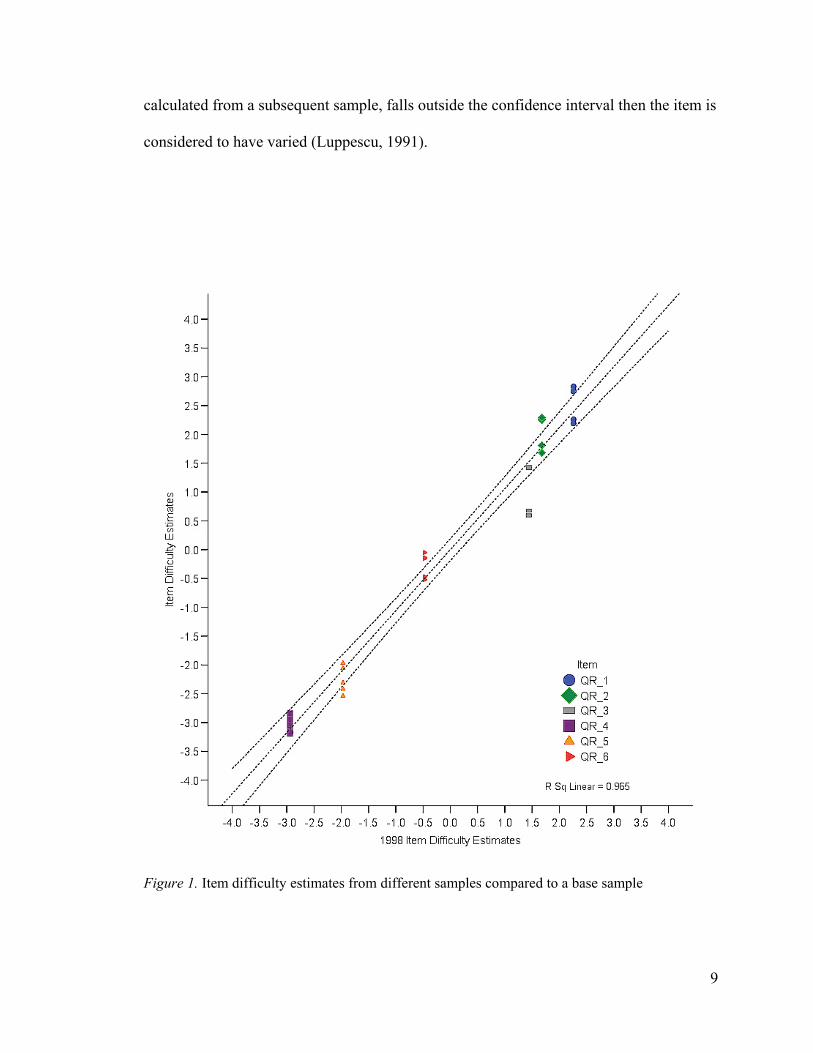
9

calculated from a subsequent sample, falls outside the confidence interval then the item is

considered to have varied (Luppescu, 1991).

Figure 1. Item difficulty estimates from different samples compared to a base sample

10

An example of variation is item QR_6 where several of the yearly item difficulty

estimates fall outside the calculated confidence interval. One shortcoming of this method

is that the standard error is influenced by the size and distribution of the groups being

compared. For this reason an additional comparison was made using the Rasch between-

fit statistics (Smith, 2004).

The second method of comparing multiple samples is performed by calculating the

item difficulty parameters for each distinct sample and computing a t-statistic that

compares the two different difficulty estimates for each item. In the separate calibration

t-test approach for two groups the items are considered invariant if the observed value of

the t-statistic is less than ± 2.0 (Gonin, Cella & Lloyd, 2001). Similarly, the calculation

of the between-fit statistic for multiple groups also creates a t-statistic that would also be

considered invariant when it is less than ± 2.0 (Smith, 2004). In Figure 2, The X-axis

represents the base group measures of the item difficulty parameters and the Y-axis

represents the t-statistic value. None of the items in Figure 2 would be considered to

have varied since they all fall inside the acceptable t-statistic parameter.

Of the two methods proposed (confidence interval and between-fit statistic), the

between-fit approach should provide the most reliable results in that it has more power to

accurately detect differences between the samples (Smith & Suh, 2003). The between-fit

approach results should be less sensitive to large sample sizes than the confidence

interval approach.

11

Figure 2. Example of between-fit t-statistics for multiple samples.

12

Item difficulty estimates. In the dichotomous Rasch model, item difficulty

estimates are calculated by dividing the proportion of people who answered the item

correctly by the percentage of people who answered the item incorrectly and then taking

the natural log of that value. This value then serves as the starting value in the Newton-

Raphson maximum likelihood estimation procedure. As explained by Bond and Fox

(2001),

The Rasch model calculations usually begin by ignoring, or constraining, person

estimates, calculating item estimates, and then using that first round of item

estimates to produce a first round of person estimates. The first round of estimates

then are iterated against each other to produce a parsimonious and internally

consistent set of item and person parameters, so that the B[person ability]-D[item

difficulty] values will produce the Rasch probabilities of success. . . . The iteration

process is said to converge when the maximum difference in item and person

values during successive iterations meets a preset convergence value. This

transformation turns ordinal-level data (i.e., correct/incorrect responses) into

interval-level data for both persons and items, thereby converting descriptive,

sample-dependent data into inferential measures based on probabilistic functions.

(p. 200)

The desirable characteristics of Rasch item and person estimates are valid only to the

degree that the data fit the model.

The Rating Scale model uses the same process as the dichotomous model to

calculate item difficulties except that an additional parameter is added that estimates the

13

probability of a respondent selecting a particular response category (e.g., well versus very

well) over the previous category in the ordinal list. The step or threshold value represents

the point on the ability scale where the conditional probability of choosing one response

category over the previous one is 50/50. The Rating Scale model estimates a step value

for each ordered pair of response categories (e.g., the first and second response

categories, the second and third response categories, etc.) A scale with five response

categories will have four threshold or step values to be estimated (Wright & Masters,

1982). Bond and Fox (2001) provide the following description of the Rasch Rating Scale

model.

The general form of the rating scale model expresses the probability of any person

choosing any given category on any item as a function of the agreeability of the

person and the endorsability of the entire item i (Di) at the given threshold K (Fk).

(p. 203)

Research Questions

This study addressed three research questions:

1. What proportion of the item difficulty estimates for each subscale of the BYU

Alumni Questionnaire are invariant when the estimates obtained from a

single-year are compared to estimates obtained from a combined multi-year

sample (all years are treated as a single administration and a single

population)? Consideration will be made for Type I error rates that may be

influence the results due the multiple comparisons between the years (Smith

2004).

14

2. What proportion of the Rasch difficulty parameters for items on the BYU

Alumni Questionnaire is invariant when a single year’s estimates are

compared to the base year estimates?

3. To what extent are item-difficulty estimates invariant for demographic

subgroups (gender, type of major) of the population across the multiple

administrations of the questionnaire? Curtin, Sudweeks, and Smith (2002)

identified items on the constructs being studied that exhibited DIF for gender,

type of major, and an interaction between gender and type of major. This test

will control for these variables to see if any item differences identified are

due to pre-existing DIF or an indication of variance in the item parameter.

Scope

This study was limited to testing for invariance of Rasch item difficulty parameter

estimates over multiple administrations of the Brigham Young University Alumni

Questionnaire. In addition, the study was limited to analyzing only 6 of 24 scales that

appear on the BYU Alumni Questionnaire. The six selected scales include the following:

1. Quantitative reasoning

2. Technology use

3. Thinking habits

4. Desire and skills needed for life-long learning

5. Physical, emotional and mental health

6. Relationships with others

These scales were chosen due to a previous study (Curtin, Sudweeks, & Smith 2001) and

known information about the presence of DIF for items in the scales.

15

Tests for invariance of the person ability parameter estimates were not examined

in this study. In order to test the invariance of the person ability parameter, each person

would need to complete the questionnaire more than once. Since the existing data sets

include responses from only a single administration to each person, testing of the person

ability estimates was not possible.

16

Chapter 2: Literature Review

This review looks at research done where the Rasch basic model assumptions are

met. It focuses on studies where the data meet the condition that the items are scored

dichotomously. Studies included should address specifically the stability (lack of

significant change) in item difficulty parameter estimates from one sample of respondents

to another. A search of electronic databases including ERIC, EBSCO, ProQuest Digital

Dissertations, SSCI, and Medline containing journal articles, papers, conference

presentations, and dissertations was conducted. In addition to these sources, the search

engine Google was used to search the World Wide Web for any additional sources such

as Rasch Measurement Transactions. The search parameters used consisted of the

keyword Rasch in combination with one or more of the following: item parameter, item

drift, invariance, stability, and person-free. Searches looked for keyword matches in both

the abstracts and the titles of the source. The Social Science Citation Index was used in

attempt to find articles or research that cited the earlier relevant publications.

Literature Review Findings

Example 1. In chapter 5 of their book, Bond and Fox (2007) discuss the

importance of invariance in measurement parameters and why it is a valuable and

necessary trait when conducting research in the human sciences. They use the analogy of

a thermometer in asserting that in order for a measurement device to be useful, the device

(instrument) should be sufficiently (a) appropriate, (b) accurate (c) precise and (d)

consistent. In the analogy of a thermometer, they illustrate the point that the thermometer

should be appropriately designed to measure the temperature of the sample (e.g., air,

17

water, metal). The thermometer should be accurate in that the measured results match the

actual conditions. The thermometer should be sufficiently precise so that it provides

measurement values useful for decision making. Finally, the thermometer should be

consistent in that it provides the same value when measurements are taken under similar

conditions (invariant across samples). Bond and Fox (2007) make the following

statement regarding the problem with measures in the human sciences:

The problem in human sciences is that many measures are not consistent

(invariant) from one data sample to another: Interpretations of results from many

tests must be made exactly in terms of the sample on which the test was normed

and the candidates’ results for tests of common human abilities depend on which

test was actually used for the estimation. This context-dependent nature of

estimate in human science research, both in terms of who was tested and what test

was used, seems to be the complete antithesis of the invariance we expect across

thermometers and temperatures. (p. 70)

Rasch measurement models provide a method that computes item difficulty

estimates that are sample independent and person ability estimates that are item

independent when appropriate samples (samples that meet the intended measurement

purpose or design) are used. The independence of the person and item estimates is

critical in meeting one of measurement goals in human sciences. “An important goal of

early research in any of the human sciences should be the establishment of item difficulty

values for important testing devices such that those values are sufficiently invariant for

their intended purposes” (Bond & Fox, 2007 p.70). The invariant property of the item

difficulty estimates allows for valid comparisons between groups of respondents. Bond

18

and Fox illustrate these measurement principles using data taken from the dichotomously

scored BLOT (Bond’s Logical Operations Test).

Example 2. One of the earliest studies of invariance in Rasch model parameter

estimates was conducted by Wright in 1967 using dichotomously scored items. His study

analyzed the responses of 628 law students participating in a test of reading

comprehension. The students were classified into two contrasting groups. The “dumb”

group consisted of students who scored 23 or below, while the “smart” group consisted of

students who scored 33 and above on the test. This design was created to create a worst

case scenario for test calibration with two very distinct groups of respondents. Using test

scores obtained from these two groups, items were calibrated across the respondents to

estimate item difficulties. These difficulty measures were then applied to all applicants

and it was demonstrated mathematically through log transformation of the log odds ratio

how the items functioned appropriately for all person ability levels. Wright concluded,

“When observations are made in terms of dichotomies like right/wrong, success/failure,

then it is a mathematical fact that this [Rasch model] is the only model which leads both

to person-free test calibration and to item-free person measurement” (1968, p.16). He

further concluded that the item difficulty estimates were invariant across both groups of

students.

Example 3. The second study was conducted by Dong, Colarelli, and Sung from

the Ball Foundation and Elizabeth Rengel (1983) from the University of Minnesota. This

study used the Ball Aptitude Battery of tests administered to three samples of high school

students: (a) 353 freshmen, (b) 112 seniors, and (c) the same 112 seniors four years later.

The Ball Aptitude Battery consists of three sections of questions: (a) inductive reasoning,

19

(b) paper folding, and (c) vocabulary. All of the test areas met the assumptions of the

Rasch model including dichotomous scoring of the items. The authors claimed that the

strength of this study was that it utilized samples of disparate ability levels. They

concluded that their findings confirmed the findings of previous studies by showing that

the Rasch estimates were invariant across groups with different abilities regardless of the

type of knowledge or skill being tested.

Example 4. The study conducted by Tinsley and Dawis (1975) examined data

obtained from four samples. These samples were (a) college students enrolled in an

introductory psychology class who completed 1,404 test booklets (each student had the

option to complete up to three test booklets), (b) high school students enrolled in two

suburban Twin Cities high schools (484 booklets), (c) civil service clerical employees of

the City of Minneapolis (289 booklets), and (d) 90 clients of the Minnesota State

Division of Vocational Rehabilitation. The samples were similar in race, religion, and

sex composition. The tests used included (a) a 60-item word analogy test, (b) a 60-item

number analogy test, (c) a 50-item picture analogy test, and (d) a 40-item symbol analogy

test. The items on each of the tests were all dichotomously scored and met the

requirements of the Rasch model. The data in this study were edited to eliminate

respondents who appeared to be careless or who did not respond to a significant number

of consecutive items. The study also tested the items for goodness of fit. Any misfitting

items were removed from further analysis.

The results of this study were consistent with the previous studies. “It was

hypothesized that Rasch ability estimates are invariant with respect to the ability of the

20

calibrating sample. The results of each of the ten comparisons support this hypothesis”

(Tinsley & Dawis, 1975, p.18).

Example 5. Smith and Suh (2003) compared the ability of Rasch statistics such as

the (a) INFIT statistic, (b) item OUTFIT statistic, (c) separate calibration t-statistic, and

(d) between-fit statistic to tests for violations of the invariance property of the item

parameter estimates. This study utilized data from a dichotomously scored, eighty-item

test that measured mathematical competency. Smith and Suh found that there were large

differences in the ability of the statistics to identify items that were not invariant. In one

case, using the between-fit statistic, they identified 69 of the 80 items on the test as

having significantly different item difficulty calibrations.

They concluded that the between-fit statistic was the most sensitive to items that

violate the invariance property of the Rasch model. They attribute the violation of the

invariance property to data that does not meet the requirements of the Rasch model.

They warn that violations of the invariance properties of item or person estimates can

have severe consequences especially in the areas of test equating or computer adaptive

testing.

Literature Review Discussion

The need and value of invariant item estimates in human science research is

introduced by Bond and Fox (2007) as previously discussed. Chapter 5 makes a

compelling argument for the need to have estimates that are invariant across appropriate

samples so that the resulting values have meaning and context. Items that have variable

difficulty estimates (sample dependent) create confounding effects where the person

ability can only appropriately be compared to others in the same sample. Bond and Fox,

21

like the subsequent studies, use dichotomous test data to illustrate the invariance property

of the Rasch model.

The assumption that item difficulty measures are independent (person-free) and

stable measures has been tested several times using dichotomous data. This was done in

the form of a mathematical proof in the case of Wright’s study and calculations of

correlated Z scores in the case of the Dong, Colarelli, Sung, and Rengel (1983) study and

in the Tinsley and Dawis (1975) study. All three studies demonstrated that the item

parameter estimates are invariant from one sample to another when the data meet the

requirements of the Rasch model. The Embretson and Reise (2000) text also provides a

mathematical argument which supports the claimed invariant nature of the Rasch item

difficulty parameter. The fourth study, Smith and Suh (2003), found that when the data

did not fit the model, item difficulty estimates were not invariant on a high school

mathematical competency test.

In recent years the Rasch model has been extended to include Andrich’s (1978a,

1978b) Rating Scale model and Masters’ (1982) Partial Credit model. These models use

polytomous scoring, such as Likert scales or graduated scoring, in place of dichotomous-

type scoring.

Other studies that have been conducted assess the impact of time when external

factors influence the stability of item parameters. Wells, Subkoviak, and Serlin (2002)

concluded that changes to the content and emphasis of curriculum can result in changes

to the difficulty of the items making some items easier and others more difficult. Stahl,

Bergstom, and Shneyderman, (2002) along with Cizek (1999) found that items may be

overexposed due to heavy usage or cheating. Additionally, Witt, Stahl, Bergstrom, and

22

Muckle (2003) found that changes in laws, policies, or regulations can affect item

difficulties. Finally, Jones, Smith, Jenson, and Peterson (2004) suggested that repeated

exposure and continuous availability of items can lead to item parameter drift over time.

All of these studies used dichotomously scored data in their analysis.

Searches of databases for journal articles, paper presentations and doctoral

dissertations did not reveal any studies investigating the stability of the item difficulty

parameter when dealing with polytomously scored data for different sample populations.

The use of self-report, Likert scale data to measure latent traits of persons creates a need

to verify the extension of the invariance of the Rasch item difficulty estimates to

polytomous scored data.

23

Chapter 3: Method

Instrument

The BYU Alumni Questionnaire consists of 207 polytomously scored items

designed to measure the effectiveness of the institution in achieving the desired student

outcomes defined in the Aims of a BYU education (BYU, 1995). The items on the

questionnaire are grouped into 24 scales. Each scale represents one of 24 unidimensional

traits identified as a desirable outcome of a BYU education. The scales use one of three

different sets of Likert response categories: (a) a five-point, describes me now; (b) a

four-point, confidence; or (c) a four-point, competence response set. Four of the six

scales that were selected for analysis in this study: (a) Uses Sound Thinking Habits;

(b) Physical, Emotional and Mental Health; (c) Possesses the Desire and Skill needed for

Life-Long Learning; and (d) Relationships with Others use the describes me now set of

response categories. The other two constructs, (e) Quantitative Reasoning and (f) Uses

Technology Effectively, are measured using the competence set of response categories.

Two forms of the questionnaire were distributed. Each alumnus was randomly assigned

to complete one of the two forms. Most items on the scales used in the study appear on

both forms of the questionnaire (Appendix A). The exceptions are (a) six of thirteen

items on the Lifelong Learning scale did not appear on both forms (Table A1), (b) one

out of ten items on the Thinking Habits scale did not appear on both forms (Table A4),

and (c) four out of six items on the Quantitative Reasoning scale did not appear on both

forms (Table A6). The distribution of items and the wording of the items were constant

over the five years of data gathered with the exception of Item 5 on the Thinking Habits

scale (Table A4).

24

Sample

The data used for this study were obtained from alumni who received their

undergraduate degree between the years 1998 and 2002 inclusively and responded to the

BYU Alumni Questionnaire. Data from the questionnaire is collected annually from

alumni three years post graduation. Respondents were classified into one of three groups

based on their type of major at the time of graduation: (a) alumni who graduated from

the College of Humanities or the College of Fine Arts and Communications (Liberal

Arts), (b) alumni who graduated from the Colleges of Physical and Mathematical

Sciences, Engineering and Technology, or Biological and Agricultural Sciences (Science)

and (c) all alumni not otherwise classified (Other).

Analysis

Responses to the Alumni Questionnaire were analyzed using Winsteps® to

compute the Rasch item difficulty statistics and IPARM® to compute between-fit

statistics. The preliminary analysis consisted of calculating item difficulty estimates for

three groupings of the data: (a) data from all five years combined, (b) data from first year

(1998), and (c) data for each individual year from 1998 to 2002.

Comparisons were made between Group A (combined years) and Group C

(individual years) and Group B (base year) to Group C. The first comparison (Group A

and Group C) is a test to see if the item difficulty parameter for a sample population is

invariant to an overall population parameter. This comparison assumes that the value for

Group A represents the entire population of BYU undergraduate degree recipients and

each year is a sample of that population. The second comparison (Group B and Group

25

C) uses data from 1998 alumni to compute anchor values. Data from each of the

subsequent years (1999-2002) were then compared against the anchored values. The

second comparison will help to identify the invariant nature of the item parameter over

time (from a base year to the subsequent years). Additional analyses were completed

using sub-grouping of data based on major type (liberal arts versus science, male versus

female). The purpose of these tests was to control for possible differences in items that

were previously identified as being subject to DIF based on gender, type of major or an

interaction of the gender and type of major (Curtin, Sudweeks, & Smith, 2002).

All analyse of the data were conducted using the computer programs Winsteps

and IPARM to calculate item difficulty estimates and between-fit statistics. The between-

fit procedure allows all groups (years) and combinations of groups (e.g., years, type of

major and gender) to be tested simultaneously for differences in the item parameters.

Differences between the groups were classified as significant when the between-fit

statistic (expected value of zero) was greater than 2.0 (Smith, 1991). Analysis of sub-

group data was accomplished using output data files from Winsteps and SPSS statistical

software.

26

Chapter 4: Results

A breakdown of respondents to the BYU Alumni Questionnaire indicates that

the samples are fairly consistent in their gender and type of major breakdown from one

year to another (Table 1).

Table 1 Distribution of Respondents by Year, Major Group, and Gender

Distribution of Respondents by Year, Major Group, and Gender

Cohort year Group Gender 1998 1999 2000 2001 2002 Total Liberal Arts Female 65% 67% 66% 68% 70% 67%

Male 35% 33% 34% 32% 30% 33% Total 505 613 580 584 437 2,719

Science Female 40% 40% 40% 40% 38% 40% Male 60% 60% 60% 60% 62% 60% Total 496 652 611 656 470 2,885

Other Female 67% 67% 68% 63% 61% 66% Male 33% 33% 32% 37% 39% 34% Total 1,202 1,397 1,371 1,404 1,020 6,394

Combined 2,203 2,662 2,562 2,644 1,927 11,998

Research Question 1

Rasch between-fit statistics were used to answer Research Question 1: What

proportion of the item difficulty parameters on each subscale of the BYU Alumni

Questionnaire are invariant when the estimates obtained from a single-year are compared

to estimates obtained when the data from all five years is combined and treated as a

27

single administration and a single population? These statistics were computed through a

number of steps that involved (a) identifying and removing misfitting persons from the

combined data set using Winsteps person fit parameters; (b) computing the item difficulty

measures on the adjusted data set with Winsteps; (c) computing item step parameters for

each of the response categories; and (d) creating an IPARM control file using the item

difficulty measures and step parameters from Winsteps for the between-fit analysis. The

IPARM analysis used five random samples of 2000 alumni to calculate a between-fit

statistic for each item. The between-fit results for each of the five random samples were

averaged to compute the between-fit statistic used for analysis (Appendix B).

The between-fit statistic for the years analysis was considered significant

based on the Bonferroni adjustments for each scale as indicated in Table 2. The

adjustment is based on the number of items in each scale (Smith, 1994). This adjustment

to the significance threshold is necessary to control the overall Type I error rate at .05.

Table 2 Bonferroni Adjustment to Critical Values for Each Scale

Bonferroni Adjustment to Critical Values for Each Scale

Scale Number of Items

Adjusted Significance

New t value

Lifelong Learning 13 .004 2.89

Physical, Emotional, & Mental Health 8 .006 2.73

Relationships with Others 6 .008 2.64

Thinking Habits 10 .005 2.81

Technology Use 6 .008 2.64

Quantitative Reasoning 6 .008 2.64

28

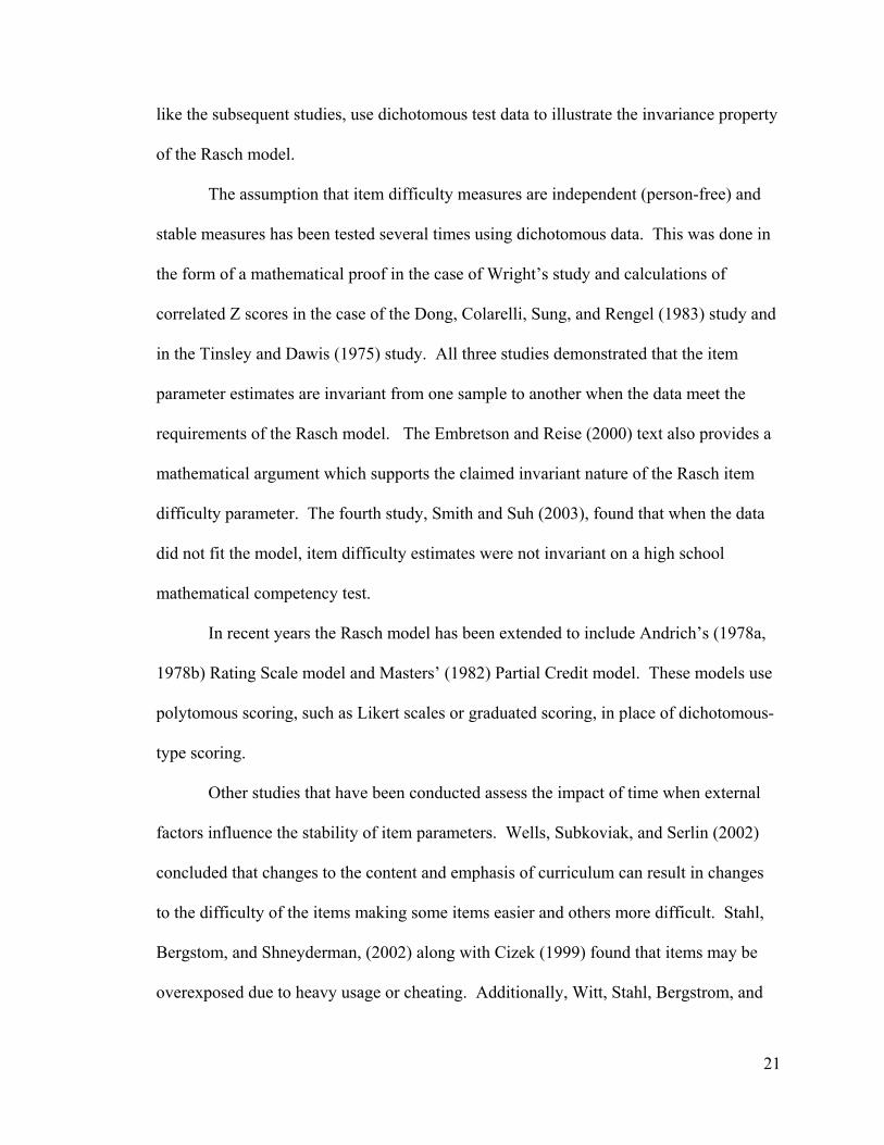
Lifelong Learning. This scale uses 13 items to measure a person’s affinity to

principles of life-long learning. The between fit approach indicates that the items in this

scale did not vary significantly in their difficulty from one year to another when

compared to difficulty estimates that were computed using the responses from all five

years (Figure 3).

Figure 3. Between-fit statistics for items on the Lifelong Learning scale.

Note. T critical = ± 2.89

29

Physical, Emotional & Mental Health. This construct consists of eight

questions that are designed to measure a person’s attitude and practices concerning

personal health. The results of this analysis identified none of the eight items as having

variance between the years estimate and the pooled estimates (Figure 4).

Figure 4. Between-fit statistics for items on the Physical, Emotional, and Mental Health

scale.

Note. t critical = ± 2.73

30

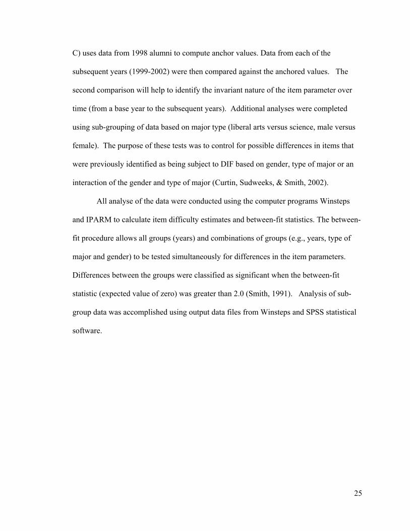
Relationship with Others. This construct has six questions that are designed to

measure how well a person relates to other people. The between-fit approach using item

estimates based on the pooled sample did not identify any of the six items as showing

variance between the individual years (Figure 5).

Figure 5. Between-fit statistics for items on the Relationship with Others scale


31

Thinking Habits. The Thinking Habits scale was developed to measure aspects of

a person’s critical thinking process. The scale contains ten items and uses a five point

“describes me well” set of response options. All of the ten items are invariant between

the individual years and the pooled difficulty estimate (Figure 6.)

Figure 6. Between-fit statistics for items on the Thinking Habits scale


32

Uses Technology Effectively. The Uses Technology Effectively scale uses a four-

point competence scale that asks respondents six questions that evaluate their own

abilities with regards to various types of technology available today. Two of the six

items (33%) indicated variation that exceeded the critical value (Figure 7).

Figure 7. Between-fit statistics for items on the Uses Technology Effectively scale


33

Quantitative Reasoning. The Quantitative Reasoning scale asks respondents to

evaluate their competence in conducting activities in the areas of math and statistics.

This scale displayed the most amount of variation. The between-fit statistic for three out

of six items (50%) exceeded the critical value (Figure 8).

Figure 8. Between-fit statistics for the Quantitative Reasoning scale.


34

Summary. For the six scales analyzed, there were a total of 5 items out of 49

(10%) that indicated significant variation in the Rasch item difficulty estimates.

Conversely, 44 of 49 items (90%) showed no statistically significant variations in their

Rasch difficulty estimates. All five items where significant variation was observed come

from two scales: (a) Technology Use and (b) Quantitative Reasoning. This may be an

indication that the source of variation is due to some issue with the scales and/or changes

in the population over time.

Research Question 2

Two methods were used to answer the second research question: What proportion

of the Rasch difficulty parameters for items on the BYU Alumni Questionnaire is

invariant when a single year’s estimates are compared to a base year estimate? The first

method used the IPARM between-fit statistics that were computed based on item

difficulty estimates and step values calibrated from the 1998 data set. As in Research

Question 1, the IPARM analysis used five random samples of 2000 alumni to calculate a

between-fit statistic for each item. The between-fit results for each of the five random

samples were averaged to compute the between-fit statistic used in the analysis

(Appendix C). The same adjustments made to the critical t values in research Question 1

were applied to this analysis.

For the second method, separate item difficulty estimates were computed for each

of the five years of respondents. The individual year estimates (Y axis) were plotted

against the estimates for the 1998 (X axis) base year. A confidence interval was plotted

around the mean of the item difficulty estimates. The confidence interval around the

estimates was computed at the 99.9% level instead of a 95% level to approximate the

35

same confidence level adjustment to critical values that was used in the between-fit

approach.

Lifelong Learning. The between-fit statistic on the Lifelong Learning scale did

not identify any items where the fit statistic was greater than the ±2.89 critical value

(Figure 9). In contrast, using confidence intervals, 14 of 65 item difficulty estimates

(22%) fall outside of the confidence bands (Figure 10).

Figure 9. Between-fit statistics for the Lifelong Learning scale using 1998 calibrations


36

Figure 10. Confidence interval results for the Lifelong Learning scale

37

Physical, Emotional and Mental Health. This scale has 2 of 8 items (25%)

categorized as showing significant variation between 1998 base year estimates and

subsequent year estimates using the IPARM between-fit statistic (Figure 11). This

compares to 8 of 40 observations (20%) having at least one year’s estimate fall outside

the confidence interval computed around the mean of the item difficulty estimates (Figure

12).

Figure 11. Between-fit statistics for the Physical, Emotional, and Mental Health scale

using 1998 calibrations


38

Figure 12. Confidence interval results for the Physical, Emotional, and Mental Health

scale

39

Relationships with Others. The Relationship with Others scale contains six items.

The between-fit statistic categorizes 1 of the 6 items (17%) as varying significantly from

the 1998 estimates over time (Figure 13.). By comparison, 8 of 30 observations (27%)

fall outside of the confidence interval (Figure 14.).

Figure 13. Between-fit statistics for the Relationship with Others scale using 1998

calibrations


40

Figure 14. Confidence interval results for the Relationship with Others scale

41

Thinking Habits. The results for the Thinking Habits scale indicate none of the 10

items are classified as varying significantly using the between-fit method when the items

are calibrated to 1998 difficulty estimates (Figure 15). This compares to 16 of 50

observations (32%) that fall outside of the 1998 confidence bands (Figure 16).

Figure 15. Between-fit statistics for the Thinking Habits scale using 1998 calibrations


42

Figure 16. Confidence interval results for the Thinking Habits scale

43

Technology Use. None of the items on the Technology Use scale are categorized

as displaying variance using the between-fit statistic (Figure 17) compared to 40% (12 of

30) using confidence intervals (Figure 18).

Figure 17. Between-fit statistics for the Uses Technology Effectively scale using 1998

calibrations


44

Figure 18. Confidence interval results for the Uses Technology Effectively scale

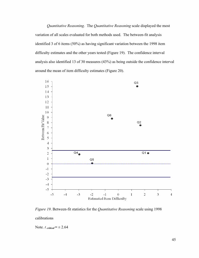
45

Quantitative Reasoning. The Quantitative Reasoning scale displayed the most

variation of all scales evaluated for both methods used. The between-fit analysis

identified 3 of 6 items (50%) as having significant variation between the 1998 item

difficulty estimates and the other years tested (Figure 19). The confidence interval

analysis also identified 13 of 30 measures (43%) as being outside the confidence interval

around the mean of item difficulty estimates (Figure 20).

Figure 19. Between-fit statistics for the Quantitative Reasoning scale using 1998

calibrations


46

Figure 20. Confidence interval results for the Quantitative Reasoning scale

47

Summary. Comparisons of item difficulty estimates of a base year to subsequent

years suggest that the difficulty estimates change over time and can be significantly

different than the base year estimate. The between-fit statistic identified 6 (12%) of 49

items as having item difficulty estimates that significantly varied between the years. The

confidence intervals categorized 71of 245 observations (29%) significantly different item

estimates from the base year estimate (Table 3).

Table 3 Count of Items with Significant Variation

Count of Items with Significant Variation

Scale Number of Items

Confidence Interval

Between Fit

Lifelong Learning 13 14 of 65 0

Physical, Emotional & Mental Health 8 8 of 40 2

Relationships with Others 6 8 of 30 1

Thinking Habits 10 16 of 60 0

Technology Use 6 12 of 30 0

Quantitative Reasoning 6 13 of 30 3

Total 49 71 of 245 6 Note. cFive item estimates (one per years) for each item on the scale.

48

Research Question 3

The General Linear Model (GLM) was used to answer Research Question 3: To

what extent are item-difficulty estimates invariant for demographic subgroups (gender,

type of major [group]) of the population across the multiple administrations of the

questionnaire? The GLM used a model with the variables of gender, type of major

(limited to science and liberal arts majors) and all possible two-way and three-way

interactions as independent variables. The Winsteps residual value for each person on

each item was used as the dependent variable in the model.

The items test for invariance on the subgroups (gender and group) over multiple

administrations focuses on the significance of year and interactions of the other

parameters with year. The assumption is that if the year parameter is not significant then

the previously identified differences between genders or type of major are also invariant

over time.

Lifelong Learning. The GLM identified only one item (Item 13) where the

variable year had a main effect. One item (10) showed an interaction effect due to gender

and year, two items (1 and 10) displayed an interaction effect for year and group, and one

item (6) had an interaction effect for gender, year, and group. Overall, 6 of 13 items

(46%) showed significant variation that could be attributed to the difference in the sample

year or an interaction with the sample year. None of the variables or interactions

accounted for much of the variance in the residuals. The maximum adjusted R-squared

value observed for the variables and interactions between the variables was less than one

percent (.009) of the variance (Table 4).

49

Table 4 Probability Estimates Produced by the GLM Model for the Lifelong Learning Scale Probability Estimates Produced by the GLM Model for the Lifelong Learning Scale f

Item Gender Year Group

Gender by

Year

Gender by

Group

Year by

Group

Gender by

Year by

Group Adjusted

R2 1 .580 .180 .004 .057 .556 .029 .787 .004

2 .132 .377 .293 .610 .601 .318 .116 .000

3 .000 .718 .502 .541 .456 .984 .133 .004

4 .000 .476 .558 .437 .011 .511 .780 .004

5 .522 .490 .951 .463 .890 .102 .527 .000

6 .000 .159 .274 .175 .192 .909 .044 .004

7 .000 .929 .003 .212 .795 .306 .517 .004

8 .000 .112 .072 .757 .319 .935 .509 .009

9 .000 .542 .382 .358 .777 .864 .682 .007

10 .000 .494 .032 .045 .251 .008 .099 .009

11 .938 .641 .226 .178 .646 .138 .673 .000

12 .005 .193 .658 .438 .678 .798 .312 .001

13 .078 .032 .397 .460 .618 .426 .114 .002

A Bonferroni post-hoc analysis indicated that the variance in the residual

attributable to Year for Item 13 was only significant between the mean of the 1998 group

of respondents and the mean of the 2000 respondent group (p = 0.031) (Appendix D).

Physical, Emotional, and Mental Health. The GLM model for the Physical,

Emotional and Mental Health scale did not identify any item where a main effect for

50

years or interactions involving years was significant. The only variables that had a main

effect in predicting the value of the Rasch person residual were gender and group. No

interactions were identified as being significant. The maximum amount of variance

accounted for in the model is found on Item 3 with an adjusted R-squared value of .034

(Table 5).

Table 5 Probability Estimates Produced by the GLM Model for the Physical, Emotional and Mental Health Scale. Probability Estimates Produced by the GLM Model for the Physical, Emotional and

Mental Health Scale


Gender by

Year

Gender by

Group

Year by

Group

Gender by

Year by

Group Adjusted

R2 1 .042 .066 .149 .644 .993 .311 .827 .001

2 .141 .812 .110 .592 .421 .925 .527 -.001

3 .000 .312 .000 .469 .878 .232 .727 .034

4 .042 .805 .044 .131 .482 .283 .396 .002

5 .001 .873 .040 .525 .721 .149 .975 .002

6 .059 .859 .896 .218 .241 .581 .202 .000

7 .000 .281 .000 .652 .932 .697 .059 .005

8 .000 .886 .015 .481 .330 .827 .824 .009

51

Relationships with Others. GLM analysis of the Relationships with Others scale

resulted in only two items (1 and 5) having a significant main effect for Year and one

item with a significant main effect for Year by Group at the .05 level. The maximum

amount of variance in the residual parameter explained by the model using gender, year,

group and their interactions was less than 4% as indicated by a maximum adjusted R

squared value of .038 (Table 6).

Table 6 Probability Estimates Produced by the GLM Model for the Relationships with Others Scale. Probability Estimates Produced by the GLM Model for the Relationships with Others

Scale


Gender by

Year

Gender by

Group

Year by

Group

Gender by

Year by

Group Adjusted

R2 1 .000 .029 .287 .651 .271 .336 .938 .005

2 .000 .356 .750 .733 .571 .485 .757 .029

3 .000 .200 .638 .378 .027 .025 .861 .038

4 .000 .116 .538 .503 .247 .295 .851 .015

5 .000 .021 .455 .677 .063 .729 .901 .019

6 .882 .665 .488 .811 .861 .056 .539 .000

The post-hoc analysis of the item on the Relationship with Others scale

revealed that the variance attributable to Year for Item 1 was only significant different

between the 1998 and 2001 cohorts (p=030) (Appendix E). The variance attributable to

52

Year for Item 5 is only significant between the 1998 and the 2000 cohorts (p = .037)

(Appendix F).

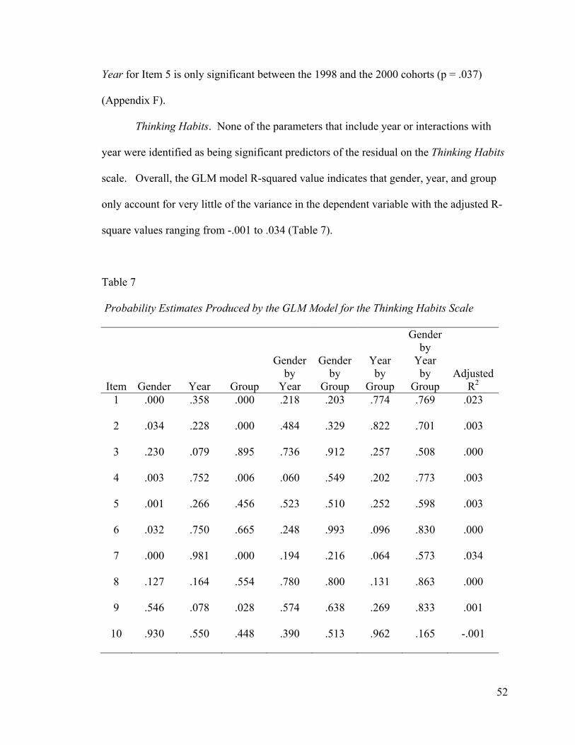
Thinking Habits. None of the parameters that include year or interactions with

year were identified as being significant predictors of the residual on the Thinking Habits

scale. Overall, the GLM model R-squared value indicates that gender, year, and group

only account for very little of the variance in the dependent variable with the adjusted R-

square values ranging from -.001 to .034 (Table 7).

Table 7 Probability Estimates Produced by the GLM Model for the Thinking Habits Scale. Probability Estimates Produced by the GLM Model for the Thinking Habits Scale


Gender by

Year

Gender by

Group

Year by

Group

Gender by

Year by

Group Adjusted

R2 1 .000 .358 .000 .218 .203 .774 .769 .023

2 .034 .228 .000 .484 .329 .822 .701 .003

3 .230 .079 .895 .736 .912 .257 .508 .000

4 .003 .752 .006 .060 .549 .202 .773 .003

5 .001 .266 .456 .523 .510 .252 .598 .003

6 .032 .750 .665 .248 .993 .096 .830 .000

7 .000 .981 .000 .194 .216 .064 .573 .034

8 .127 .164 .554 .780 .800 .131 .863 .000

9 .546 .078 .028 .574 .638 .269 .833 .001

10 .930 .550 .448 .390 .513 .962 .165 -.001

53

Technology Use. The Technology Use scale did not have any items where the year

parameter was significant (either by itself or as part of an interaction parameter) in the

linear model. Gender and the type of major (group) are the parameters in the model that

play the most significant role in predicting the residual value. The values of gender, year,

and group account for less than 1% of the variance in the residual values for five of the

six items and only accounted for 2% of the variance in item 2 based on the adjusted R-

squared statistic (Table 8).

Table 8 Probability Estimates Produced by the GLM Model for the Technology Use Scale Probability Estimates Produced by the GLM Model for the Technology Use Scale


Gender by

Year

Gender by

Group

Year by

Group

Gender by

Year by

Group Adjusted

R2 1 .000 .217 .045 .310 .979 .838 .116 .003

2 .000 .337 .525 .788 .747 .057 .529 .021

3 .000 .340 .006 .369 .986 .207 .149 .007

4 .000 .751 .206 .372 .011 .255 .580 .007

5 .000 .344 .042 .551 .133 .227 .105 .005

6 .003 .745 .001 .132 .975 .557 .887 .002

Quantitative Reasoning. The GLM analysis of the Quantitative Reasoning scale

revealed the most significant variance between subgroups over time based on four of the

six items (1, 2, 3, and 6) having a significant effect for the year parameters and one of the

items (3) also indicating a significant effect for the interaction of gender and year. None

54

of the items in the scale are significant for the interaction between year and group or year,

gender, year and group. While several of the items identified significant relationships

between the year parameter and the dependent (residual) variable. The parameters in the

GLM accounted for less than 3% of the variance with adjusted R-squared values ranging

from .000 to .027 (Table 9).

Table 9 Probability Estimates Produced by the GLM Model for the Quantitative Reasoning Scale Probability Estimates Produced by the GLM Model for the Quantitative Reasoning Scale

Item Gender Year Group Gender by Year

Gender by

Group Year by Group

Gender by Year

by Group

Adjusted R2

1 .000 .008 .000 .149 .234 .070 .736 .022

2 .001 .000 .144 .783 .036 .291 .900 .011

3 .001 .000 .291 .001 .291 .426 .524 .027

4 .000 .065 .105 .171 .021 .185 .281 .007

5 .250 .223 .003 .757 .822 .745 .623 .000

6 .540 .000 .641 .715 .327 .115 .970 .009

The Bonferroni post-hoc tests for Item 1 indicate that the significant differences

for item 1 are between the 1999 and 2000 cohorts ( p=004) (Appendix G). The

differences in Year for Items 2 and 3 are between the 1998 and 2000 (p=.000) cohorts,

the 1998 and 2001 (p=.000) cohorts, and the 1998 and 2002 (p=.000) cohorts (Appendix

H and I). The difference in Year for item 6 were not only between the 1998 and the 2000-

2002 cohorts, but also the 1999 and the 2000-2002 cohorts (p ≤ .001) (Appendix J).

55

Summary. Overall, the interaction of year with the other demographic

subgroups does not appear to be a major contributor of variance in the item estimates.

Only the year by type of major (group) interaction had more than 5% of the items on all

six scales identified as being significant in the linear model. The interaction for the

subgroup gender and year identified only two of the total 49 items (4%) as significant in

predicting the residual value. The interaction of the demographic subgroups gender and

type of major (group) with year was identified only one time out of the 49 items (2%) as a

significant parameter in the linear model (Table 10). Since a 95% confidence level was

used, these results in the GLM fall near or within the range of expected error when

looking at the variance of demographic subgroups over time.

56

Table 10 Count of Items Where Year or an Interaction with Year was Significant

Count of Items Where Year or an Interaction with Year was Significant

Scale Items Year

Gender by

Year

Year by

Group

Gender by

Year by

Group Unique Items

Lifelong Learning 13 1 1 2 1 4

Physical, Emotional, and Mental Health

8 0 0 0 0 0

Relationships with Others 6 2 0 1 0 3 Thinking Habits 10 0 0 0 0 0 Technology Use 6 0 0 0 0 0 Quantitative Reasoning 6 4 1 0 0 4 Total 49 7 2 3 1 11

Percent 14% 4% 6% 2% 22%

57

Chapter 5: Conclusions and Recommendations

Research Question 1

The first research question addresses the robustness of the Rasch model item

difficulty parameter estimates and whether or not the estimates are invariant (do not

change significantly) from one sample to the next when the samples are selected from the

same population of real data. To test this claim, all respondents for the five years were

pooled together to calculate item difficulty calibrations. The yearly administrations of

the AQ were used to identify the distinct samples and the between-fit statistic was used to

identify items that varied from year to year. The results of this analysis indicated that 5

of 49 (10%) items had significant variation in their item difficulty estimates across the

years. While this is higher than the .05 Type I error rate, it is important to note that all 5

items that were identified as variant were contained in two scales. The Quantitative

Reasoning scale contained three of the six items that varied between the years and the

Technology Use scale contained the other two variant items. Three scales did not contain

any items where the item difficulty estimates varied significantly across the years. These

scales included the following:

1. Physical, Emotional, and Mental Health

2. Lifelong Learning

3. Relationships with Others

The fact that some scales had items that varied across years and other scales did not may

be an indication that the observed variance is due to issues within the scales themselves

and not the Rasch model. This test did not consider possible confounding variables such

58

as the impact of gender or type of major. Hence, it is possible that the observed variance

is due to these confounding factors and not differences in the annual sample.

Research Question 2

The second research question was designed to assess the degree of variation in

item difficulty estimates when a base year’s estimate is compared to independently

calibrated estimates from subsequent years. Two methods were used to analyze the data:

a confidence interval around the mean of the estimates and between-fit statistics when

compared to the base year item difficulty estimates.

The results of this analysis indicated that there is more variation in item parameter

estimates when subsequent years are compared to a base year. Using the confidence

interval method, 71 of the 241 item estimates computed (29%) were classified as lying

outside their respective confidence bands. By comparison, the between-fit statistic

identified 6 items (12%) as having variance between the base year and the subsequent

years. Both methods had variance rates larger than can be explained by expected Type I

error rates. The results of this test are an indication of possible item parameter drift (IPD)

in the item estimates.

As in the results computed for the first research question, the confidence intervals

and the between-fit statistic computed did not take into consideration other sources of

variation such as gender and type of major. This approach also assumes that the sample

used in the base year estimates are comparable to the samples used in subsequent years.

Research Question 3

The third research question was designed to assess the degree of variation in the

item difficulty estimates between the yearly samples when the effects of the confounding

59

variables of gender and type of major are taken into consideration. The GLM controlled

for groups of years, gender, major and all possible interactions between these three

independent variables (Appendix K). The dependent variable in the model was the raw

residual (i.e., the observed score minus the expected score) for each respondent on each

item. Linacre (1998) demonstrated the raw residuals are more sensitive to the presence

of multidimensionality than alternatives and states, “The raw score residuals, however,

most directly reflect the presence of any other dimensions” (p. 271).

Compared to the results observed in research questions one and two, the GLM

identified the fewest number of items where there was a significant amount of variance

attributable to the year variable. Of the 49 items on the six scales, seven (14%) had a

significant effect for year. Four of the seven items, where year was a significant

predictor, were on the Quantitative Reasoning scale. Three of the six scales did not have

any items where year or an interaction with year was a significant parameter in the

model. When considering year and the interactions of year, gender, and type of major, a

total of 11 (22%) had some variance that was attributable at least in part to year.

The parameter that is most frequently classified as a significant source of variance

is gender followed by the type of major. The significance of gender and type of major on

the scales was expected due to earlier DIF studies on the 1998 cohort (Curtin, Sudweeks,

& Smith, 2002). The lack of significant interaction effect between gender, type of major

and year would indicate that the item estimates are invariant for subgroups of respondents

over the years.

An advantage of the GLM method is that it computes an estimate of the

proportion of the total variance that is explained by each source of variation. Analysis of

60

the R-squared values indicates that the model parameters never accounted for more than

4% (.038) of the variance in the residuals for any item.

The results of the analysis for the third research question support the claim of the

Rasch model that the item estimates are invariant for different samples of a population.

The amount of variance observed on some scales for gender and type of major supports

the conclusion that for some scales, the different genders or different majors should be

considered distinct populations.

Method Comparison

The three methods, (a) between-fit, (b) confidence intervals, and (c) the general

linear model, used to identify variation in item difficulty estimates all provide useful

information. The between-fit statistics and the GLM both classified approximately the

same proportion of the items as having varied from one sample to another (Table 11).

while proportion of variation for the confidence interval approach was over twice as large

as any of the other methods (Table 12).

61

Table 11 Comparison of Methods Used to Identify Variation Between Years

Comparison of Methods Used to Identify Variation Between Years

Number of items having significant variation

between years

Between Fit General Linear Model

Scale Number of items

Calibrated to pooled estimates

Calibrated to 1998

estimates Year

Year by

gender

Year by

type of

major

Year by

gender by

type of

major Lifelong Learning

13 0 0 1 1 2 1

Physical, Emotional & Mental Health

8 0 2 0 0 0 0

Relationships with Others

6 0 1 2 0 1 0

Thinking Habits

10 0 0 0 0 0 0

Technology Use

6 2 0 0 0 0 0

Quantitative Reasoning

6 3 3 4 1 0 0

Count 49 5 6 7 2 3 1

Percent 10% 12% 14% 4% 6% 2%

62

Table 12 Variation Between Years Using Confidence Intervals

Variation Between Years Using Confidence Intervals

Confidence Interval

Violations

Scale Number of

items

Observations (Items * Years) Count Percent

Lifelong Learning 13 65 14 22%

Physical, Emotional & Mental Health

8 40 8 20%

Relationships with Others

6 30 8 27%

Thinking Habits 10 50 16 32%

Technology Use 6 30 12 40%

Quantitative Reasoning

6 30 13 43%

Total 49 245 71 29%

The between-fit statistic allows for simultaneous comparisons between up to five

separate groups of respondents. Since the between-fit statistic calculated is comparable

to a t-statistic, the researcher is able to make adjustments to the critical value to control

the Type I error rate. One possible disadvantage of the between-fit statistic is an issue of

power. The between-fit statistic is able to identify small differences in groups, the larger

the groups (sample size) the greater the difference. The power of the between-fit statistic

can lead to errors of interpretation of identified differences when large samples are used.

63

Another drawback to the between-fit statistic is that it does not identify changes in

difficulty order between the items.

The confidence interval method using separate calibrations of the item difficulty

estimates for groups provides a quick, visual representation of differences between the

comparison groups. The graphical display of the data also allows for checks to see if

there are changes in the order of the item difficulties from one year to the next. The main

flaw with the confidence interval approach is that it is very easily influenced by sample

size. Large samples result in small confidence intervals which in turn result in a higher

number of items being classified as significantly different. The inflated Type I errors in

the analysis could lead to faulty conclusions. The dependence on visuals can also make

interpretation difficult when the items lie close together and the confidence bands are

narrow. This can lead to different interpretations of the same graph by different

individuals.

The GLM offers the ability to control for more subgroups of respondents than the

between-fit method. Where the between-fit method in the IPARM program allows for a

maximum of five groups, the GLM method allows for an unlimited number of groups.

The GLM also has available to it post-hoc analysis that can aid in identifying sources of

variance. The GLM also provides the adjusted R-squared statistics that are useful when

considering the practical significance of the variance observed.

Conclusion

The results of the three research questions provide insight into the overall

question regarding the assumption of sample invariance of item difficulty parameters in

the Rasch rating scale model. The first research question resulted in 10% of the items

64

classified as variant. The second research question classified between 12% and 29% of

the items as having varied. The GLM had 14% of the item classified as variant based on

the different year samples. These results are all above an expected Type I error rate of

5%. However, in the between-fit and the GLM models the majority of the items

identified as having varied came from the quantitative reasoning scale.

If the Quantitative Reasoning scale is removed, then, only two or three of the

remaining 43 items are classified as not being invariant (4.6 – 6.9%) depending on the

method used. Without the items in the Quantitative Reasoning scale, the number of

items that vary are at or near the expected 5% error rate. The assumption that the

remaining items are due to Type I error is supported in the random nature of the

classification of the remaining items. None of the items that varied on the other scales

were identified in more than one of the methods used to test for invariance. In contrast,

all methods used classified Items 3 and 6 of the Quantitative Reasoning scale as having

varied over years, both the GLM and the between-fit (1998) approach classified Item 2 as

varied and the GLM and the between-fit (all) approaches classified Item 1 on the

Quantitative Reasoning scale as having varied more than what would be expected due to

sampling error. This may be an indication that the variation observed in the Quantitative

Reasoning scale is due to problems with the scale or the administration of the items and

not the Rasch model.

The confidence interval approach is difficult to assess in that identifying items as

varied can be subjective, especially when the intervals are tight around the mean and

significant differences result from small changes in item estimates. Even the size of the

symbol used to identify the measure adds a certain degree of error in the interpretation of

65

the graph. When used with more than two comparison groups, it appears that the

confidence interval method may not yield sufficiently clear results to make accurate

decision about difference in groups. The ambiguity of the results makes any analysis

subject to increased amounts of error due to both errors in the measurements and the

interpretation of the plots.

The GLM method provides insight into the true nature of the variance observed

throughout the study. Neither Research Question 1 nor Research Question 2 controlled

for known differences between respondents based on their gender or type of major. The

GLM controlled for both of these factors and revealed that the interaction between the

year (sample), gender and type of major resulted in only one item (2%) as having varied

significantly. This is below the 5% Type 1 error rate. Further analysis shows that the

most commonly significant factors in the model were gender and type of major. These

findings suggest that on some of these scales there are distinct populations being

measured. When the samples come from the same population (gender and type of major)

then the item estimates are invariant across sample (year). The results from the GLM

support the claim of the Rasch model that item estimates for polytomously scored items

are invariant across samples.

Recommendation for Practice

The results of this study confirm the value of Rasch Rating Scale model when

conducting longitudinal studies using polytomously scored data. This study highlights

the fact that there are often real differences between sub-populations of students and that

these differences can and should be anticipated depending on the construct being

measured. When these differences are anticipated, then comparisons should only be

66

made between samples of these sub-groups when attempting to identify change. When

using the Rasch model it is not only important to make sure that the items are measuring

a unidimensional trait but also are measuring a homogeneous population with respect to

the construct.

The study supports the invariant nature of the Rasch item difficulty parameter

estimates when the data fit the model and come from repeated samples of the population.

The invariant nature of the item difficulty estimates makes them useful in conducting

longitudinal studies. Invariant item difficulties makes it possible to assess the impact of a

new treatment or program on desired traits without the confounding effects of

measurement issues.

Based on the results from the three research questions, the between-fit statistic is a

useful tool when there are five groups or less to compare. Like the GLM, the between-fit

statistic offers limited ability to check for interactions between variables. The confidence

interval approach is useful only for a quick, high level test of variation and provides a

visual check for any changes in the difficulty order of the items. The results of the

confidence interval approach should be used with caution due to the sensitivity of the

critical values to sample size and the propensity of the conclusions to be affected by the

researcher (rater effect). The most versatile approach when testing variation between

samples is the GLM.

The GLM method for detecting variation has several benefits, such as (a) it allows

the researcher to control for as many for variables as they want, (b) it provides post-hoc

analysis to identify the source of the variation and (c) it computes R-squared statistics

that indicate the proportion of the total amount of variance that can be contributed to the

67

variables in the model. The R-squared statistic is a valuable tool for the researcher when

trying to identify which variables, if any, create the greatest amount of variation.

Once the source or cause of any significant variance (variance not due to

sampling error) is identified, then appropriate steps can be taken to create either better

items or more homogeneous populations. For example, the results on the BYU AQ

indicate that males and females should be considered separate populations for some of

the scales and data for these two groups (males and females) should be analyzed

separately. Likewise the problems identified with missing data on the Quantitative

Reasoning scale can be addressed by including all items on the scale on both forms of the

questionnaire.

Recommendations for Further Research

Two additional issues discovered through the course of this study warrant further

investigation. These issues deal with the impact of (a) sample size on between-fit

statistic and the confidence interval bands and (b) the impact of missing data.

The impact of sample size was observed on both the between-fit statistics and the

confidence interval methods. Large samples create small standard errors that resulted in

extremely small confidence bands around the mean if the item estimates. These

extremely small confidence bands result in more items being classified as displaying

variation. Likewise when large sample were used with the between-fit approach,

differences between groups were magnified. Previous studies for between-fit statistics

have typically involved sample sizes smaller than 2,000. In this study the data set

consisted of over 11,000 respondents which resulted in unusually large between-fit

statistics.

68

Research should be conducted that will evaluate the impact of different sample

sizes on both the confidence intervals and the between-fit statistic. The goal of this

research would be to identify the (a) minimum, (b) maximum and (c) optimal sample size

for analysis that will yield dependable and valid results.

A second issue observed in this study dealt with the impact of missing data. The

Quantitative Reasoning scale displayed the most variation of all of the scales studied.

This scale was unique in that a person is only presented with four of the six items on the

scale. Only two of the six items are answered by all respondents (Table A6). The result

of the design for the administration of this scale is that 33% of the item data is missing

for any given person and 50% of the data is missing on four of the six items.

The large amount of systematic missing data on the Quantitative Reasoning scale

that is not present on the other scales may be one reason why the scale performed poorly.

Additional research should be conducted that examines the impact of missing data on the

between-fit statistic, the GLM model and confidence bands. The goal of this research

would be to identify limits to the proportion of acceptable missing data as well as create

measures that identify the overall impact of the missing data on the stability of the item

estimates. The research should also look at the differences on how the available software

(e.g., IPARM, SPSS, Winsteps) handle missing data during the calculation of the various

statistics.

69

References

Andrich, D. (1978a). Application of a psychometric rating model to ordered categories

which are scored with successive integers. Applied Psychological Measurement,

2, 581-594.

Andrich, D. (1978b). A rating formulation for ordered response categories.

Psychometrika, 43, 561-573.

Bond, T.G., & Fox, C.M. (2001). Applying the Rasch model: Fundamental measurement

in the human sciences. Mahwah, NJ: Lawrence Erlbaum Associates

Bond, T.G., & Fox, C.M. (2007). Applying the Rasch model: Fundamental measurement

in the human sciences (Second edition). Mahwah, NJ: Lawrence Erlbaum

Associates

Brigham Young University (1995) Aims of a BYU education. Retrieved November 9,

2006 from http://unicomm.byu.edu/about/aims/?lms=1

Cizek, G.L. (1999). Cheating on tests: How to do it, detect it, and prevent it. Mahwah,

NJ: Lawrence Erlbaum.

Curtin, J.A., Sudweeks, R.R, & Smith, R.M. (2002, April). Analyzing DIF in polytomous

responses of university alumni to a follow-up questionnaire, Paper presented at

the annual meeting of the American Educational Research Association, Chicago,

IL.

Dong, H., Colarelli, S.M., Sung, Y.H., & Rengel E. (1983, August). An empirical

investigation of sample-free calibration claim of the Rasch model. The Ball

Foundation Technical Report, No. 11.

70

Embretson, S.E., & Reise, S.P. (2000). Item response theory for psychologists. Mahwah,

NJ: Lawrence Erlbaum Associates.

Engelhard, G. Jr. (1994). Historical views of the concept of invariance in measurement

theory. In M. Wilson (Ed.), Objective measurement: Theory into practice, (vol. 2,

pp. 73-99), Norwood, NJ: Ablex.

Gonin R., Cella D., & Lloyd S. (2001). Differential item functioning. Rasch

Measurement Transactions, 15(3), 838. Retrieved June 15, 2006, from

http://rasch.rog/rmt/rmt153j.htm

Jones, P., Smith, R., Jenson, E., & Peterson G. (2004, April). Item parameter drift in

small-volume continuously available non-adaptive computerized certification

tests in the information technology industry. Paper presented at the annual

meeting of the National Council of Measurement in Education, San Diego, CA.

Linacre J.M. (1998). Detecting multidimensionality: Which residual data-type works

best? Journal of Outcome Measurement 2. 266-283.

Luppescu, S. (1991). Graphical diagnosis. Rasch Measurement Transactions, 5:(1), 136

Retrieved June 15, 2006 from http://www.rasch.org/rmt/rmt51j.htm

Masters, G.N. (1982). A Rasch model for partial credit scoring. Psychometrika, 47, 149-

174

Osterlind, S.J. (2006). Modern measurement: Theory, principles, and applications of

mental appraisal. Upper Saddle River, NJ: Pearson Merrill Prentice Hall.

Stahl, J.A., Bergstrom, B.A., & Shneyderman. (2002, April). Impact of item drift on test-

taker measurement. Paper presented at the annual meeting of the American

Educational Research Association, New Orleans.

71

Smith, R.M. (1991). IPARM: Item and person analysis with the Rasch model. Chicago:

MESA Press.

Smith, R.M. (1994). A comparison of the power of Rasch total and between-item fit

statistics to detect measurement disturbances. Educational and Psychological

Measurement 54, 42-55.

Smith, R.M. (2004). Fit analysis in latent trait measurement models. In E.V. Smith Jr.

and R.M. Smith (Eds.), Introduction to Rasch measurement: Theory, models and

applications (pp. 73-92). Maple Grove, MN: JAM Press.

Smith, R.M., & Suh, K.K. (2003) Rasch fit statistics as a test of the invariance of item

parameter estimates. Journal of Applied Measurement 4, 153-163.

Tinsley, H. E.A., & Dawis, R.V. (1975). An investigation of the Rasch simple logistic

model: Sample-free item and test calibration. Educational and Psychological

Measurement, 35, 325-339.

Wells, C.S., Subkoviak, M.J., & Serlin, R.C. (2002). The effect of item parameter drift

on examinee ability estimate. Applied Psychological Measurement, 26, 77-87

Witt, E.A., Stahl, J.A., Bergstrom, B.A., Muckle, T. (2003, April). Impact of item drift

with non-normal distributions. Paper presented at the annual meeting of the

American Educational Research Association, Chicago, IL.

Wright B.D. (1996a). Comparisons Require Stability, Rasch Measurement Transactions

10(2), 506. Retrieved June 15, 2006 from http://www.rasch.org/rmt/rmt102p.htm

Wright B.D. (1996b). Key events in Rasch measurement history, Rasch Measurement

Transactions 10(2), 494-496. Retrieved July 28, 2006 from

http://www.rasch.org/rmt/rmt102q.htm

72

Wright B.D., & Masters, G.N. (1982). Rating scale analysis. Chicago, IL: Mesa Press.

Wright, B.D. (1968). Sample-free test calibration and person measurement. Proceedings

of the 1967 Invitational Conference on Testing Problems. Princeton, NJ:

Educational Testing Service. (ERIC Document Reproduction Service No.

ED017810)

73

Appendix A

Item Maps for the Various Alumni Questionnaire Scales

74

Table A1 Distribution of Items by Form for the Lifelong Learning Scale

Distribution of Items by Form for the Lifelong Learning Scale

Item Indicate how well each of the following statements describes you now.

Form A

Form B

LL_1 I regularly explore new interests and ideas. X

LL_2 When I study, I consciously choose or create an environment conducive to learning.

X X

LL_ 3 I persist in searching for solutions to unsolved problems in spite of previous failures.

X

LL_4 I consistently enjoy learning new skills and ideas. X X

LL_5 I accept responsibility for my own learning, including what I have learned incompletely or incorrectly.

X X

LL_6 I correctly assess my own individual learning needs. X

LL_7 I consistently seek to clarify ideas that I don’t understand. X

LL_8 I select and use different learning strategies (e.g. flash cards, practice, study sessions) to match what I am trying to learn.

X X

LL_9 I strive to develop new skills to keep up with change. X

LL_10 I regularly monitor and evaluate the processes I use to study so that I can adjust them in order to learn more effectively.

X X

LL_11 I allocate adequate time for accomplishing learning tasks. X

LL_12 I am willing to consider new information or interpretations, even when they contradict my own position on an issue.

X

LL_13 I consciously try to improve my skills and develop new abilities so that I can serve more effectively.

X

75

Table A2 Distribution of Items by Form for the Physical, Emotional & Mental Health Scale Distribution of Items by Form for the Physical, Emotional & Mental Health Scale


Form A

Form B

PEMH_1 I regularly engage in physical exercise.

X X

PEMH_2 I consistently maintain a health-conscious diet.

X X

PEMH_3 I live by principles of good general health (e.g., regular medical checkups, following sound medical advice, staying informed about healthy lifestyle practices).

X X

PEMH_4 I incorporate sound mental and emotional health practices into my lifestyle (e.g. recreation, adequate sleep).

X X

PEMH_5 I have at least one personal friend in whom I can confide.

X X

PEMH_6 I balance my work with appropriate recreational activities.

X X

PEMH_7 I take time daily for personal reflection or meditation.

X X

PEMH_8 I am generally satisfied with my life.

X X

76

Table A3 Distribution of Items by Form for the Relationships with Others Scale

Distribution of Items by Form for the Relationships with Others Scale

Item Indicate how well each of the following statements describes you now

Form A

Form B

RWO_1 I have positive relationships outside of my family which I have maintained for 3-5 years.

X X

RWO_2 I am confident in my ability to interact with other people in a variety of social situations.

X X

RWO_3 I gain personal, emotional, or spiritual strength from my relationships with other people.

X X

RWO_4 I find personal satisfaction in my relationships with other people.

X X

RWO_5 I make friends easily. X X

RWO_6 I am sensitive to the fact that my choices and actions influence the lives of other people.

X X

77

Table A4 Distribution of Items by Form for the Thinking Habits Scale

Distribution of Items by Form for the Thinking Habits Scale


Form A

Form B

TH_1 I regularly seek and weigh evidence before drawing conclusions.

X X

TH_2 I refrain from taking a strong position on an issue when evidence is insufficient.

X X

TH_3 I give serious and fair-minded consideration to points of view advocated by others.

X X

TH_4 I habitually evaluate my own assumptions, conclusions, and reasoning.

X X

TH_5 When people try to persuade me to change my point of view, I typically analyze their reasoning and question their assumptions and conclusions

X X

TH_6 I try to find relationships between what I am learning and what I already know.

X X

TH_7 I try to relate new things I learn to my own experience. X X

TH_8 I willingly acknowledge my mistakes when my thinking is shown to be flawed or incomplete.

X X

TH_9 I willingly acknowledge biases or inconsistencies in my own thinking.

X X

TH_10 I am willing to consider new information or interpretations, even when they contradict my own position on an issue.

X

Note. The wording for Item 5 changed beginning with the 1999 cohort. The 1998 alumni

responded to Item 5 written as: I regularly question the assumptions, conclusions, and

reasoning offered by others.

78

Table A5 Distribution of Items by Form for the Uses Technology Effectively Scale

Distribution of Items by Form for Uses Technology Effectively Scale

Item How competent are you in your ability to…? Form

A Form

B TU_1 Use information technologies (e.g. CD-ROMs, internet,

electronic library indexes, etc.) to aid your study and learning

X X

TU_2 Stay informed about developments in computing technology (e.g., word processing, graphics, communication, presentations)

X X

TU_3 Use basic office technology (e.g. computer, fax machine, e-mail)

X X

TU_4 Use technology tools to enhance learning, increase productivity, and promote creativity

X X

TU_5 Evaluate and select new information resources and technological innovations based on their appropriateness for specific tasks

X X

TU_6 Use technology resources for solving problems and making informed decisions

X X

79

Table A6 Distribution of Items by Form for the Quantitative Reasoning Scale

Distribution of Items by Form for the Quantitative Reasoning Scale

Item How competent are you in your ability to…? Form

A Form

B QR_1 Compute and use descriptive statistics (means and standard

deviations) to summarize numerical data

X X

QR_2 Recognize misuses of mathematical and statistical reasoning

X

QR_3 Make and test inferences about the characteristics of a population based on information obtained from a sample

X

QR_4 Correctly interpret quantitative information presented in graphs and charts in newspapers, magazines, books, and advertisements, etc.

X X

QR_5 Evaluate the arguments you encounter in newspapers, magazines, books, at work, or elsewhere that are based on analysis of quantitative data

X

QR_6 Construct arguments to support a conclusion you have reached based on analysis of numerical data

X

80

Appendix B

Summary of Between-fit Statistics from 5 Random Samples Anchored to Complete Set of

Respondents

81

Table B1 Lifelong Learning Between-fit statistics

Lifelong Learning Between-fit Statistics

Sample Group

Item 1 2 3 4 5 M SD

1 0.85 0.64 0.35 2.05 - 0.25 0.73 0.85

2 - 0.90 - 1.07 0.56 0.67 0.33 - 0.08 0.84

3 0.43 0.53 0.60 0.42 0.90 0.58 0.20

4 - 1.48 1.49 0.58 - 0.17 1.57 0.40 1.27

5 0.39 - 0.45 0.46 - 0.59 0.63 0.09 0.56

6 - 0.12 0.69 - 1.12 - 0.57 - 0.46 - 0.32 0.67

7 0.00 0.00 0.00 0.00 0.00 0.00 0.00

8 0.93 0.41 - 0.38 - 0.06 0.82 0.34 0.56

9 0.65 1.32 - 0.08 0.84 - 0.22 0.50 0.65

10 - 0.79 1.83 0.65 0.61 - 0.17 0.43 0.99

11 - 0.29 3.01 - 0.55 - 0.68 - 0.13 0.27 1.55

12 0.92 0.06 - 0.67 - 0.69 1.42 0.21 0.95

13 0.60 0.66 - 0.34 0.24 0.08 0.25 0.41

82

Table B2 Physical, Emotional and Mental Health Between-fit statistics

Physical, Emotional and Mental Health Between-fit Statistics

Sample Group

Item 1 2 3 4 5 M SD

1 2.27 1.02 3.42 3.03 1.38 2.22 1.03

2 - 0.88 0.85 0.71 - 1.50 0.94 0.02 1.13

3 1.78 - 0.25 - 0.31 2.18 - 0.86 0.51 1.37

4 - 0.71 - 0.15 - 0.81 0.19 - 0.16 - 0.33 0.42

5 - 0.09 - 1.86 0.48 1.36 - 0.31 - 0.08 1.18

6 - 1.12 0.04 - 0.82 - 0.48 - 1.52 - 0.78 0.60

7 1.56 1.19 1.98 1.65 2.70 1.82 0.57

8 - 1.87 - 0.85 0.26 1.68 - 0.80 - 0.32 1.35

Table B3 Relationships with Others Between-fit Statistics

Relationships with Others Between-fit Statistics

Sample Group

Item 1 2 3 4 5 M SD

1 - 0.61 1.47 2.26 2.24 - 0.21 1.03 1.36

2 0.75 - 0.62 - 0.16 - 0.68 - 1.31 - 0.40 0.76

3 1.10 0.41 0.50 0.63 0.95 0.72 0.30

4 1.77 0.75 1.75 - 1.22 0.87 0.78 1.22

5 2.65 0.67 0.88 4.29 3.25 2.35 1.55

6 0.12 0.76 1.92 0.08 - 0.90 0.40 1.04

83

Table B4 Thinking Habits Between-fits Statistics

Thinking Habits Between-fits Statistics

Sample Group

Item 1 2 3 4 5 M SD

1 0.95 0.24 1.06 1.09 - 0.04 0.66 0.52

2 0.00 1.73 - 0.15 0.52 0.96 0.61 0.76

3 - 0.12 0.71 0.51 0.99 0.22 0.46 0.43

4 1.52 1.92 - 0.36 - 0.72 - 0.05 0.46 1.18

5 - 2.20 0.02 0.01 0.06 2.53 0.08 1.67

6 0.38 - 1.65 - 1.19 0.17 1.46 - 0.17 1.26

7 1.33 - 2.22 0.70 0.56 1.53 0.38 1.51

8 1.89 2.15 - 0.34 2.26 1.11 1.41 1.08

9 0.58 0.86 - 0.47 1.15 - 0.76 0.27 0.84

10 0.57 0.00 - 1.81 0.46 0.85 0.01 1.06

Table B5 Uses Technology Effectively Between-fit Statistics

Uses Technology Effectively Between-fit Statistics

Sample Group

Item 1 2 3 4 5 M SD

1 0.06 0.79 - 1.25 2.73 - 0.60 0.35 1.53

2 4.71 3.30 5.79 4.31 5.02 4.63 0.92

3 0.78 - 0.07 0.84 1.20 0.92 0.73 0.48

4 0.82 1.26 0.51 1.24 - 1.65 0.44 1.21

5 3.30 4.03 3.40 3.36 3.58 3.53 0.30

6 - 0.09 0.54 0.53 0.29 1.91 0.64 0.76

84

Table B6 Quantitative Reasoning Between-fit Statistics

Quantitative Reasoning Between-fit Statistics

Sample Group Item 1 2 3 4 5 M SD

1 2.96 4.12 3.60 3.58

3.32 3.52 0.43

2 2.12 0.91 2.72 3.92

2.47 2.43 1.09

3 6.44 4.14 6.34 5.67

6.98 5.91 1.10

4 - 0.18 1.57 0.92 0.62

1.31 0.85 0.68

5 - 1.30 - 0.60 - 0.48 1.92

0.13 - 0.07 1.22

6 3.74 4.52 4.64 3.34

3.53 3.95 0.59

85

Appendix C

Between-fit Statistics from 5 Random Samples Anchored to 1998 Data

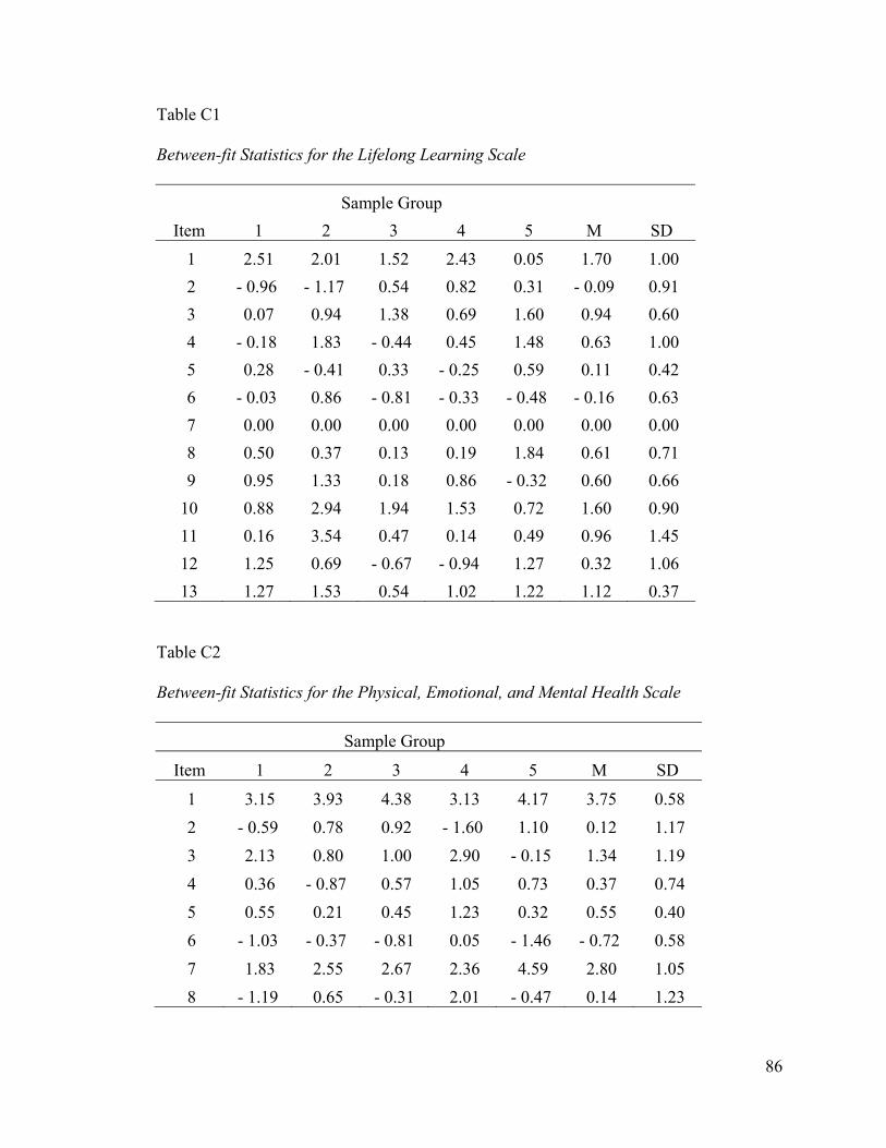
86

Table C1 Between-fit Statistics for the Lifelong Learning Scale

Between-fit Statistics for the Lifelong Learning Scale


1 2.51 2.01 1.52 2.43 0.05 1.70 1.00 2 - 0.96 - 1.17 0.54 0.82 0.31 - 0.09 0.91 3 0.07 0.94 1.38 0.69 1.60 0.94 0.60 4 - 0.18 1.83 - 0.44 0.45 1.48 0.63 1.00 5 0.28 - 0.41 0.33 - 0.25 0.59 0.11 0.42 6 - 0.03 0.86 - 0.81 - 0.33 - 0.48 - 0.16 0.63 7 0.00 0.00 0.00 0.00 0.00 0.00 0.00 8 0.50 0.37 0.13 0.19 1.84 0.61 0.71 9 0.95 1.33 0.18 0.86 - 0.32 0.60 0.66 10 0.88 2.94 1.94 1.53 0.72 1.60 0.90 11 0.16 3.54 0.47 0.14 0.49 0.96 1.45 12 1.25 0.69 - 0.67 - 0.94 1.27 0.32 1.06 13 1.27 1.53 0.54 1.02 1.22 1.12 0.37

Table C2 Between-fit Statistics for the Physical, Emotional, and Mental Health Scale

Between-fit Statistics for the Physical, Emotional, and Mental Health Scale

Sample Group

Item 1 2 3 4 5 M SD

1 3.15 3.93 4.38 3.13 4.17 3.75 0.58 2 - 0.59 0.78 0.92 - 1.60 1.10 0.12 1.17 3 2.13 0.80 1.00 2.90 - 0.15 1.34 1.19 4 0.36 - 0.87 0.57 1.05 0.73 0.37 0.74 5 0.55 0.21 0.45 1.23 0.32 0.55 0.40 6 - 1.03 - 0.37 - 0.81 0.05 - 1.46 - 0.72 0.58 7 1.83 2.55 2.67 2.36 4.59 2.80 1.05 8 - 1.19 0.65 - 0.31 2.01 - 0.47 0.14 1.23

87

Table C3 Between-fit Statistics for the Relationships with Others Scale

Between-fit Statistics for the Relationships with Others Scale


1 0.42 2.70 2.81 2.80 0.93 1.93 1.16 2 0.47 - 1.01 - 1.09 - 0.16 - 0.76 - 0.51 0.66 3 2.32 1.77 2.79 2.38 2.85 2.42 0.43 4 3.45 2.94 4.24 1.54 3.26 3.09 0.99 5 1.03 0.59 1.86 1.87 1.58 1.39 0.56 6 0.05 0.67 2.29 0.35 - 0.09 0.65 0.96

Table C4 Between-fit Statistics for the Thinking Habits Scale

Between-fit Statistics for the Thinking Habits Scale


1 1.39 0.54 1.44 1.18 0.58 1.03 0.44 2 0.05 1.71 0.67 0.87 0.71 0.80 0.60 3 0.62 0.65 1.94 2.91 0.13 1.25 1.14 4 1.94 1.93 1.65 - 0.32 - 0.70 0.90 1.30 5 - 1.81 - 0.46 1.02 0.83 1.80 0.28 1.42 6 1.14 - 0.73 - 0.88 1.27 1.52 0.46 1.17 7 1.44 - 2.51 0.94 0.55 1.65 0.41 1.69 8 3.17 2.24 1.15 1.94 - 0.09 1.68 1.23 9 0.39 0.73 - 0.11 1.21 - 0.72 0.30 0.75 10 0.63 0.00 - 1.79 0.46 0.86 0.03 1.07

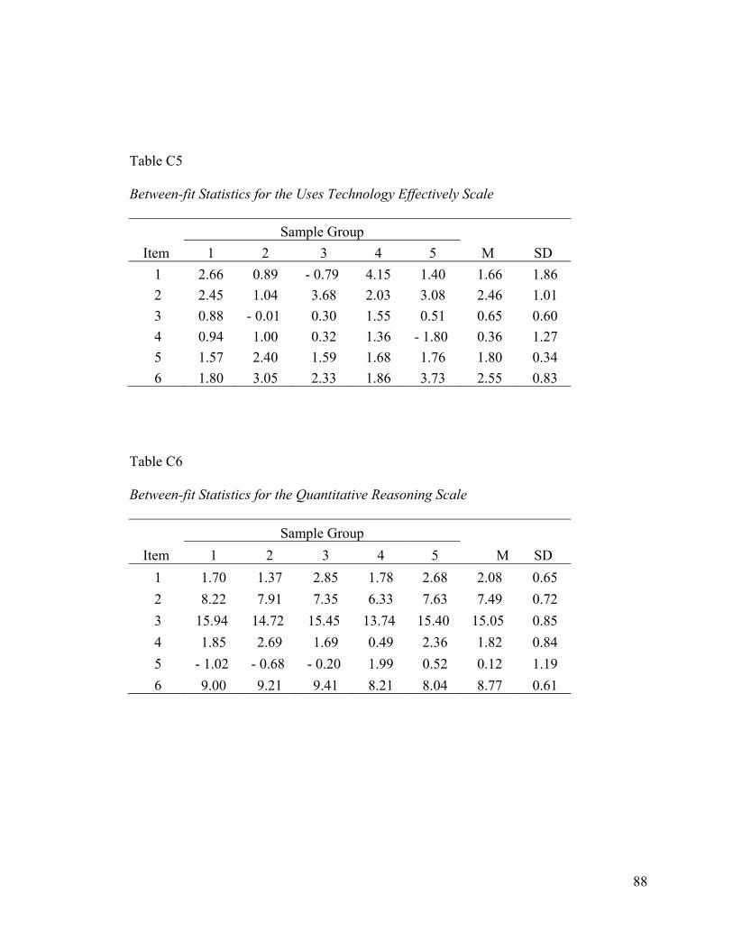
88

Table C5 Between-fit Statistics for the Uses Technology Effectively Scale

Between-fit Statistics for the Uses Technology Effectively Scale


1 2.66 0.89 - 0.79 4.15 1.40 1.66 1.86 2 2.45 1.04 3.68 2.03 3.08 2.46 1.01 3 0.88 - 0.01 0.30 1.55 0.51 0.65 0.60 4 0.94 1.00 0.32 1.36 - 1.80 0.36 1.27 5 1.57 2.40 1.59 1.68 1.76 1.80 0.34 6 1.80 3.05 2.33 1.86 3.73 2.55 0.83

Table C6 Between-fit Statistics for the Quantitative Reasoning Scale

Between-fit Statistics for the Quantitative Reasoning Scale


1 1.70 1.37 2.85 1.78 2.68 2.08 0.65 2 8.22 7.91 7.35 6.33 7.63 7.49 0.72 3 15.94 14.72 15.45 13.74 15.40 15.05 0.85 4 1.85 2.69 1.69 0.49 2.36 1.82 0.84 5 - 1.02 - 0.68 - 0.20 1.99 0.52 0.12 1.19 6 9.00 9.21 9.41 8.21 8.04 8.77 0.61

89

Appendix D

Bonferroni Post Hoc Tests for Item 13 on the Lifelong Learning Scale

90

Year (I)

Year (J)

Mean Difference

(I-J) SE p

95% Confidence Interval

Lower Bound Upper Bound1998 1998

1999 .0181 .01457 1.000 -.0229 .0590 2000 .0438 .01480 0.031 .0022 .0853 2001 .0130 .01466 1.000 -.0282 .0542 2002 .0247 .01583 1.000 -.0198 .0691

1999 1998 -.0181 .01457 1.000 -.0590 .0229

1999 2000 .0257 .01393 0.651 -.0134 .0648 2001 -.0051 .01378 1.000 -.0438 .0336 2002 .0066 .01502 1.000 -.0356 .0488

2000 1998 -.0438 .01480 0.031 -.0853 -.0022

1999 -.0257 .01393 0.651 -.0648 .0134 2000 2001 -.0308 .01403 0.282 -.0702 .0086 2002 -.0191 .01524 1.000 -.0619 .0237

2001 1998 -.0130 .01466 1.000 -.0542 .0282

1999 .0051 .01378 1.000 -.0336 .0438 2000 .0308 .01403 0.282 -.0086 .0702 2001 2002 .0117 .01510 1.000 -.0307 .0541

2002 1998 -.0247 .01583 1.000 -.0691 .0198

1999 -.0066 .01502 1.000 -.0488 .0356 2000 .0191 .01524 1.000 -.0237 .0619 2001 -.0117 .01510 1.000 -.0541 .0307 2002

91

Appendix E

Bonferroni Post Hoc Tests for Item 1 on the Relationships with Others Scale

92

Year (I)

Year (J)

Mean Difference

(I-J) SE p



1999 -.0288 .02331 1.000 -.0943 .0366 2000 -.0582 .02356 0.135 -.1244 .0079 2001 -.0692 .02336 0.030 -.1349 -.0036 2002 -.0232 .02510 1.000 -.0937 .0473

1999 1998 .0288 .02331 1.000 -.0366 .0943 1999 2000 -.0294 .02225 1.000 -.0919 .0331 2001 -.0404 .02203 0.666 -.1023 .0214 2002 .0056 .02387 1.000 -.0614 .0727

2000 1998 .0582 .02356 0.135 -.0079 .1244 1999 .0294 .02225 1.000 -.0331 .0919 2000 2001 -.0110 .02230 1.000 -.0736 .0516 2002 .0350 .02412 1.000 -.0327 .1028

2001 1998 .0692 .02336 0.030 .0036 .1349 1999 .0404 .02203 0.666 -.0214 .1023 2000 .0110 .02230 1.000 -.0516 .0736 2001 2002 .0460 .02392 0.542 -.0211 .1132

2002 1998 .0232 .02510 1.000 -.0473 .0937 1999 -.0056 .02387 1.000 -.0727 .0614 2000 -.0350 .02412 1.000 -.1028 .0327 2001 -.0460 .02392 0.542 -.1132 .0211 2002

93

Appendix F

Bonferroni Post Hoc Tests for Item 5 on the Relationships with Others Scale

94

Year (I)

Year (J)

Mean Difference

(I-J) SE p



1999 .0431 .02176 0.478 -.0180 .1042 2000 .0639 .02200 0.037 .0021 .1256 2001 .0157 .02181 1.000 -.0456 .0769 2002 .0562 .02343 0.165 -.0096 .1220

1999 1998 -.0431 .02176 0.478 -.1042 .0180

1999 2000 .0208 .02077 1.000 -.0375 .0791 2001 -.0274 .02057 1.000 -.0852 .0303 2002 .0131 .02228 1.000 -.0495 .0757

2000 1998 -.0639 .02200 0.037 -.1256 -.0021

1999 -.0208 .02077 1.000 -.0791 .0375 2000 2001 -.0482 .02081 0.206 -.1066 .0103 2002 -.0077 .02251 1.000 -.0709 .0556

2001 1998 -.0157 .02181 1.000 -.0769 .0456

1999 .0274 .02057 1.000 -.0303 .0852 2000 .0482 .02081 0.206 -.0103 .1066 2001 2002 .0405 .02233 0.695 -.0222 .1032

2002 1998 -.0562 .02343 0.165 -.1220 .0096

1999 -.0131 .02228 1.000 -.0757 .0495 2000 .0077 .02251 1.000 -.0556 .0709 2001 -.0405 .02233 0.695 -.1032 .0222 2002

95

Appendix G

Bonferroni Post Hoc Tests for Item 1 on the Quantitative Reasoning Scale

96

Year (I)

Year (J)

Mean Difference

(I-J) SE p



1999 -.0328 .01920 0.876 -.0867 .0211 2000 .0324 .01953 0.972 -.0224 .0872 2001 .0132 .01936 1.000 -.0412 .0675 2002 .0108 .02094 1.000 -.0480 .0696

1999 1998 .0328 .01920 0.876 -.0211 .0867 1999 2000 .0652 .01834 0.004 .0137 .1167 2001 .0460 .01816 0.114 -.0051 .0970

2002 .0436 .01984 0.279 -.0121 .0993 2000 1998 -.0324 .01953 0.972 -.0872 .0224

1999 -.0652 .01834 0.004 -.1167 -.0137 2000 2001 -.0192 .01851 1.000 -.0712 .0327 2002 -.0216 .02016 1.000 -.0782 .0350

2001 1998 -.0132 .01936 1.000 -.0675 .0412 1999 -.0460 .01816 0.114 -.0970 .0051 2000 .0192 .01851 1.000 -.0327 .0712 2001 2002 -.0023 .01999 1.000 -.0585 .0538

2002 1998 -.0108 .02094 1.000 -.0696 .0480 1999 -.0436 .01984 0.279 -.0993 .0121 2000 .0216 .02016 1.000 -.0350 .0782 2001 .0023 .01999 1.000 -.0538 .0585 2002

97

Appendix H


98

Year (I)

Year (J)

Mean Difference

(I-J) SE p



1999 .0336 .01256 0.075 -.0017 .0689 2000 .0640 .01278 0.000 .0281 .0999 2001 .0770 .01267 0.000 .0415 .1126 2002 .0584 .01370 0.000 .0199 .0968

1999 1998 -.0336 .01256 0.075 -.0689 .0017

1999 2000 .0304 .01200 0.115 -.0034 .0641 2001 .0434 .01189 0.003 .0100 .0768 2002 .0247 .01298 0.569 -.0117 .0612

2000 1998 -.0640 .01278 0.000 -.0999 -.0281

1999 -.0304 .01200 0.115 -.0641 .0034 2000 2001 .0131 .01211 1.000 -.0210 .0471 2002 -.0056 .01319 1.000 -.0427 .0314

2001 1998 -.0770 .01267 0.000 -.1126 -.0415

1999 -.0434 .01189 0.003 -.0768 -.0100 2000 -.0131 .01211 1.000 -.0471 .0210 2001 2002 -.0187 .01308 1.000 -.0554 .0181

2002 1998 -.0584 .01370 0.000 -.0968 -.0199

1999 -.0247 .01298 0.569 -.0612 .0117 2000 .0056 .01319 1.000 -.0314 .0427 2001 .0187 .01308 1.000 -.0181 .0554 2002

99

Appendix I


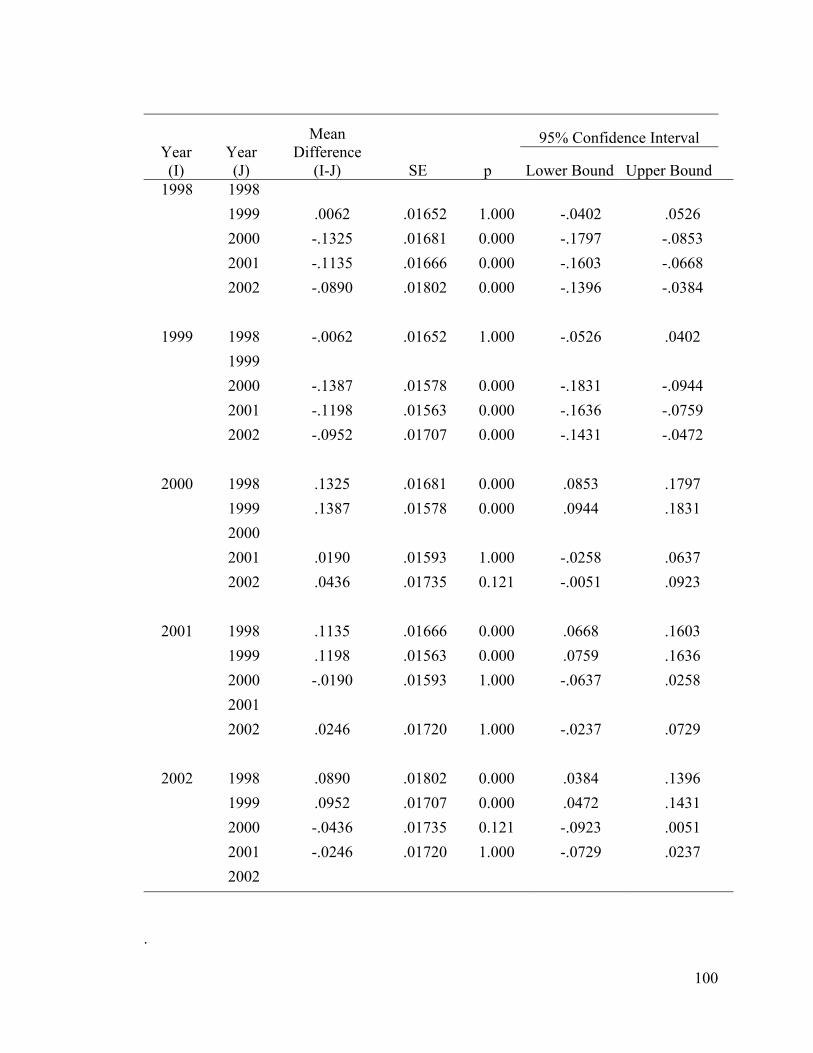
100

Year (I)

Year (J)

Mean Difference

(I-J) SE p



1999 .0062 .01652 1.000 -.0402 .0526 2000 -.1325 .01681 0.000 -.1797 -.0853 2001 -.1135 .01666 0.000 -.1603 -.0668 2002 -.0890 .01802 0.000 -.1396 -.0384

1999 1998 -.0062 .01652 1.000 -.0526 .0402

1999 2000 -.1387 .01578 0.000 -.1831 -.0944 2001 -.1198 .01563 0.000 -.1636 -.0759 2002 -.0952 .01707 0.000 -.1431 -.0472

2000 1998 .1325 .01681 0.000 .0853 .1797

1999 .1387 .01578 0.000 .0944 .1831 2000 2001 .0190 .01593 1.000 -.0258 .0637 2002 .0436 .01735 0.121 -.0051 .0923

2001 1998 .1135 .01666 0.000 .0668 .1603

1999 .1198 .01563 0.000 .0759 .1636 2000 -.0190 .01593 1.000 -.0637 .0258 2001 2002 .0246 .01720 1.000 -.0237 .0729

2002 1998 .0890 .01802 0.000 .0384 .1396

1999 .0952 .01707 0.000 .0472 .1431 2000 -.0436 .01735 0.121 -.0923 .0051 2001 -.0246 .01720 1.000 -.0729 .0237 2002

.

101

Appendix J


102

Year (I)

Year (J)

Mean Difference

(I-J) SE p



1999 -.0053 .01169 1.000 -.0381 .0275 2000 .0534 .01189 0.000 .0200 .0868 2001 .0473 .01178 0.001 .0142 .0803 2002 .0557 .01274 0.000 .0199 .0915

1999 1998 .0053 .01169 1.000 -.0275 .0381

1999 2000 .0586 .01116 0.000 .0273 .0900 2001 .0525 .01105 0.000 .0215 .0836 2002 .0609 .01207 0.000 .0270 .0948

2000 1998 -.0534 .01189 0.000 -.0868 -.0200

1999 -.0586 .01116 0.000 -.0900 -.0273 2000 2001 -.0061 .01127 1.000 -.0378 .0255 2002 .0023 .01227 1.000 -.0322 .0367

2001 1998 -.0473 .01178 0.001 -.0803 -.0142

1999 -.0525 .01105 0.000 -.0836 -.0215 2000 .0061 .01127 1.000 -.0255 .0378 2001 2002 .0084 .01217 1.000 -.0258 .0426

2002 1998 -.0557 .01274 0.000 -.0915 -.0199

1999 -.0609 .01207 0.000 -.0948 -.0270 2000 -.0023 .01227 1.000 -.0367 .0322 2001 -.0084 .01217 1.000 -.0426 .0258 2002

103

Appendix K

SPSS Commands for the GLM model.

104

COMPUTE filter_$=(GroupCode ~= 2).

VARIABLE LABEL filter_$ 'GroupCode ~= 2 (FILTER)'.

VALUE LABELS filter_$ 0 'Not Selected' 1 'Selected'.

FORMAT filter_$ (f1.0).

FILTER BY filter_$.

EXECUTE .

UNIANOVA

RESIDL BY Gender Year GroupCode

/METHOD = SSTYPE(3)

/INTERCEPT = INCLUDE

/POSTHOC = Year ( BONFERRONI )

/CRITERIA = ALPHA(.05)

/DESIGN = Gender Year GroupCode Gender*Year

Gender*GroupCode Year

*GroupCode Gender*Year*GroupCode .

testing the assumption of sample invariance of item

Documents