testing the accuracy of machine guidance in road construction

1

University of Southern Queensland

Faculty of Engineering and Surveying

Testing the Accuracy of Machine Guidance in Road

Construction

A dissertation submitted by

Mr. Said Kiongoli

In fulfilment of the requirements of

ENG 4111/4112, Research Project

towards the degree of

Bachelor of Spatial Science, Surveying

Submitted: October 2010

2

Abstract

3D Machine Control and Guidance Systems first appeared on the market in the late 1990‟s.

These systems put a small computer within the cab of earthwork machines that utilized

Global Positioning System (GPS) satellites to relay position information to the computer (see

figure 1.1). The computer evaluates the actual position relative to its location in the proposed

model. The operator uses the information from the onboard computer to control the

machine‟s equipment. In advanced cases, the onboard computer can be directly linked to the

machine hydraulics, controlling their operation with minimal input from operator.

Automated machine guidance using RTS was the major new application of this advancement

in technology. Robotic Total Stations (RTSs) were first introduced by Geodimeter in 1990.

These instruments incorporated servomotors and advanced tracking sensors which allowed

the instrument to track a target. RTS‟s are now utilized in the construction and extractive

industries for the guidance of major earthworks machinery as well as in agriculture industry

for the guidance of machinery such as tractors and harvesters.

In today‟s world, with the application of RTS, ATSs and now moving into real time AMG.

The accuracies and latency of both operations are still not well understood, it has become

critical to understand the exact accuracies that these instruments are capable of achieving

whilst operating in the field. Thus upon the completion of this project my aim is to have a

better understanding of both operational accuracies of several instruments, as well as their

performances.

The working specification in most of road construction are general requires the tolerance of

±0.02m. In order to achieve this tolerance required for such work we need to determine if

these technologies are capable of meeting such accuracies.

Upon the completion of this project, we will have a better understanding of how the

accuracies of the machine guidance works and under what conditions the contractor,

engineers or surveyors can understand the performance of the AMG works better.

5

AKNOWLEDGEMENT

The author wishes to acknowledge the support and guidance received from Dr. Albert Chong

of the University of Southern Queensland, throughout the course of the research project.

Special thanks must also be made to the following organisations and people for the provision

of equipment, facilities and guidance:

Mark Tranter and Peter Fripp of Abigroup Leightons –ALJV (Gateway Project) for

letting me do the field work and providing all the assistance I needed.

Mr Shane Simon of the University of Southern Queensland for his support and

assistance.

All the Staff and members of the University of Southern Queensland for helping me

to achieve my goals.

Said Kiongoli


October 2010

6

TABLE OF CONTENTS

Contents Page

Abstract 2

Limitation of Use 3

Certification 4

Acknowledgement 5

List of figures 10

List of table 11

List of Appendices 11

Abbreviations 12

CHAPTER 1 - INTRODUCTION

1.1 Background of research 13

1.2 Aim 14

1.3 Objective 14

1.4 Justification 14

1.5 Overview of Dissertation 15

CHAPTER 2 - LITERATURE REVIEW

2.1 Introduction 16

2.1.1 Overview of Machine Control 18

2.2 Real Time Kinematic (RTK), Global Positioning System –GPS 18

2.2.1 RTK GPS surveying 18

2.2.2 RTK receivers 18

7

2.2.3 Radio Signals 19

2.2.4 (VRS) GPS 19

2.2.5 Laser Augmented RTK GPS 19

2.2.6 Accuracy 19

2.2.7 How good is RTK GPS? 20

2.3 Trimble GCS500 and 600 Grade Control System Cross Slope Control 21

2.3.1 GCS500 Grade Control System Cross Slope Control 21

2.3.2 GCS600 Grade Control System Cross-Slope and Elevation Control 21

2.3.2.1 Trimble ST400 Sonic Tracer 21

2.4 Leica TPS 1200 22

2.4.1 Introduction 22

2:4:2 Power search (PS) 22

2:4:3 Angles 23

2.4.4 Distance measurement. 23

2.4.5 ATR 24

2.4.6 Servo Drive. 25

2.5 Trimble 5600 (ATS) Total station 25

2.5.1 ATS (Advanced Tracking Sensor) 25

2.5.2 Synchronization 26

2.5.3 Latency 26

2.5.4 Servo controls. 27

2.5.5 RMT Super Multi Channel 28

2.5.6 Distance meter Calibration. 28

2.5.7 Auto-Search 28

2.5.8 Distance 29

2.5.9 Angle measurement System. 29

2.5.10 Dual Axis Compensator 29

8

2.5.11 Collimation Errors 29

2.5.12 Trunion axis Tilt 29

2.6 Previous Tests Undertaken 30

2.6.1 – Chua 2004. 30

2.6.2 Ceryova 2002 30

2.6.3 Dennis Garget. 31

2.6.4 Conclusion. 31

2.7 RTK GPS latency in Dynamic Environment 32

2.8 Trimble ATS Evolution. 33

2.8.2 3D Positioning Accuracy. 33

CHAPTER 3 - RESEARCH APPROACH AND METHODOLOGY

3.1 Introduction 34

3.2 Data collection and testing. 35

3.2.1 - Equipment used 35

3.2.2 Main components of the instruments: 35

3.2.3 Trimble GCS600 Grade Control System 35

3.3 Project Planning. 35

3.4 Literature Contribution to Research Method 36

3.5 Field Testing. 36

3.6 Operation of RTS (leica1200), ATS (5600s) and RTK GPS 38

3.6.1 RTK GPS 38

3.6.2 Operating on GPS (AMG) 39

3.6.2 Operation of an ATS5600 (Field) 39

3.6.2.1 Setup the instrument 39

3.7 Operation of a Leica 1202 (Field) 40

Conclusion

9

CHAPTER 4 - DATA ANALYSIS AND DISSCUSSION

4.1 Introduction 41

4.2 Data Analysis 42

4.2.1 Raw data collection and Transfer 42

4.2.2 Data transfer to a personal computer 43

4.3 Software utilised and outputting data for analysis 43

4.4 Analysing the Database information 43

4.4.1 Analysing the GCS600 GPS 44

4.4.2 Analysing the Trimble ATS5600 46

4.4.3 Further Analysis for the Trimble ATS5600 and GPS grader 47

4.5 Results 61

4.5.1 CG600 GPS 61

4.5.2 Trimble ATS5600 results 66

4.6 Summary of results 70

4.7 Discussion 71

4.7.1 Reliability 71

4.7.2 Accuracy of Tracking 71

CHAPTER 5 - CONCLUSION AND RECOMENDATIONS

5.1 Introduction 72

5.2 Further Research and Recommendations 72

5.2.1 Testing GCS600 GPS 72

5.2.2 Additional device (Laser augmented RTK GPS) 72

5.2.3 Testing at Speeds 73

5.2.4 Testing Trimble ATS5600 73

10

5.3 Conclusion 73

LIST OF FIGURE

Figure 1.1: Trimble GCS900 on a Motor Grader with Dual GPS 13

Figure 2.1: the new Trimble SPS630, SPS730 and SPS930 Universal Total Stations 16

Figure 2.2: Trimble ATS 600 16

Figure 2.3: Trimble Control Unit 16

Figure 2.4: Trimble GCS900 on a Dozer with Single GPS and Laser Augmentation 16

Figure 2.5: 3D-MILLIMETER GPS+ 17

Figure 2.6: MILLIMETER GPS FOR PAVING 17

Figure 2.7: LPS-900 17

Figure 2.8: Topcon Control Unit 17

Figure 2.10: T400 Sonic Tracer 22

Figure 2.11: Synchronization 26

Figure 2.12: Latency (ATS 5600) 27

Figure 2.13: RMT ATS Multi Channel 28

Figure 3.1 Showing a plan view of the road at Gateway Project 37

Figure 4.1; Analysis process 42

Figure 4.2; Latency errors-50m interval for GPS 61

Figure 4.3 – 4.11; Latency errors-combined GPS machine runs 62 - 66

Figure 4.12, vertical errors during 50m interval check for ATS 67

Figure 4.13 – 4.18; Latency errors-combined ATS Total stations machine runs 67 - 70

11

LIST OF TABLES

Table 2.1 Manufacturer RTK equipment Specifications 20

Table 2.2; PS specifications 22

Table 2.3 TPS 1200 Series angle Accuracies (STD Dev) 23

Table 2.4 TPS Distance measurements with (IR mode) prisms-reflectors 24

Table 2.5: LEICA ATR Specifications 24

Table 2.6: ATR Range 25

Table 4.1 showing an example of database information on spreadsheet. 44

Table 4.2 showing analysis of data for Trimble GCS600, captured by leica instrument 45

Table 4.3 showing readings obtained from GPS machine operator 45

Table 4.4 COMPARISON OF DATA EXTRACTED FROM TABLE (GPS) 45

Table 4.5 showing analysis of data for Trimble ATS5600 46

Table 4.6 showing readings obtaiened from ATS machine operator 46

Table 4.7 COMPARISON OF DATA EXTRACTED FROM TABLE (ATS) 46

Table 4.8 Showing the analysis of data for Trimble GCS600 GPS 47 - 54

Figure 4.9 Showing analysis of data for Trimble ATS 5600 54 - 60

APPENDICES

APPENDIX A; Project Specification

APPENDIX B; Safe Work Method Statement and Risk Assessment

APPENDIX C; Cross Sections

APPENDIX C; Trimble ATS5600 Notes

APPENDIX D: Trimble GC600 Notes

APPENDIX E: Digital Terrain Modal (DTM or TIN

12

ABBREVIATIONS

TIN – Triangular Irregular Network

RTK – Real time Kinematic

USQ - University of Southern Queeensland

VRS – Virtual reference Station

PC – Personal Computer

GNSS – Global Position System

13


FACULTY OF ENGINEERING AND SURVEYING

ENG 4111/4112 Research Project

PROJECT APPRECIATION

CHAPTER 1

INTRODUCTION

1:1 Background of research

Automated Machine Guidance (AMG) is also known as Machine Control (MC). It‟s a

process that uses continually updating measurements from:

Robotic Total Stations (RTS)

Real Time Kinetic (RTK) Global Positioning System (GPS)

Laser System, or

Sonic System

3D Machine Control and Guidance Systems first appeared on the market in the late 1990‟s.

These systems put a small computer within the cab of earthwork machines that utilized

Global Positioning System (GPS) satellites to relay position information to the computer (see

figure 1.1). The computer evaluates the actual position relative to its location in the proposed

model. The operator uses the information from the onboard computer to control the

machine‟s equipment. In advanced cases, the onboard computer can be directly linked to the

machine hydraulics, controlling their operation with minimal input from operator.

Figure 1.1: Trimble GCS900 on a Motor Grader with Dual GPS

(Trimble, 2010)

14

The success 3D Machine control system relies upon several variables, including;

The ability of the operator to accurately apply the design in the field

The ability of the owner to approve and review the design

The quality of proposed construction model.

Automated machine guidance using RTS was the major new application of this advancement

in technology. Robotic Total Stations (RTSs) were first introduced by Geodimeter in 1990.

These instruments incorporated servomotors and advanced tracking sensors which allowed

the instrument to track a target. RTS‟s are now utilized in the construction and extractive

industries for the guidance of major earthworks machinery as well as in agriculture industry

for the guidance of machinery such as tractors and harvesters.



whilst operating in the field. Thus upon the completion of this project my aim is to have a

better understanding of both operational accuracies of several instruments, as well as their

performances.

1.2 Aims

The Aim of this project is to test the accuracy and reliability of Machine Guidance when used

in Road construction.

1.3 Objectives

1. Research the background information in relation to Machine Guidance

2. Review existing literature concerned Real time and conventional or traditional guidance

systems (ATS, RTSs).

3. Establish and conduct a series of testing under various conditions.

4. Undertaking analysis of test results, and

5. Determining the final accuracies of machine guidance systems.

1.4 Justification

In today‟s world, with the application of RTS, ATSs and now moving into real time AMG.



whilst operating in the field.

15

The working specification in most of road construction are general requires the tolerance of

±0.02m. In order to achieve this tolerance required for such work we need to determine if

these technologies are capable of meeting such accuracies.

There will be some conditions to be achieved to meet the accuracies requirements. Such

conditions are:

Distances for ATS, RTS

Angles for ATS, RTS

Speed of moving targets

Environmental obstruction on prism locks.

Number of satellites –RTK GPS

Environmental obstruction on GPS returning false answer

GPS precision

Upon the completion of this project, we will have a better understanding of how the

accuracies of the machine guidance works and under what conditions the contractor,

engineers or surveyors can understand the performance of the AMG works better.

1.5 Overview of Dissertation

The brief overview of each chapter contained in the dissertation is provided below.

Chapter 2 will be mainly used for providing conclusion and comparison with the relevant or

similar research which was investigated by any other part. It does this by providing the

following information:


2. Review existing literature concerning Real time and conventional or traditional guidance

systems (ATS, RTSs), and comment on previous test undertaken.

3. Establish and conduct a series of testing, analyse the result and determining the final

accuracies of machine guidance systems.

Chapter 3 provides detailed information into both the testing regime which has been

implemented and the data analysis methodology.

Chapter 4 will provide analysis and discussion concerning the results obtained on chapter 3.

Chapter 5 is where the conclusion will be drawn and recommendations will be presented.

16

CHAPTER 2

LITERATURE REVIEW

2.1 Introduction

In order to provide some background into the operations of Automated machine guidance, I

would like to describe briefly the mechanical workings of various forms of AMG, two or

three of them will be tested. These instruments or machines are Trimble ATS 5600 and ATS

600 TCS2 Total stations, GCS900 Universal Total Stations, Trimble GCS600 and GCS900:

Dual or single GPS + GLONASS. Topcon‟s 3D-Millimeter GPS+, Millimeter GPS for

paving. (See Figure 2):

TRIMBLE INSTRUMENTS

Figure 2.2: Trimble ATS 600

Figure 2.1: the new Trimble SPS630, SPS730 and SPS930 Universal Total Stations

Figure 2.3: Trimble Control Unit

Figure 2.4: Trimble GCS900 on a Dozer with Single GPS and Laser Augmentation

17

TOPCON INSTRUMENTS

Figure 2.5: 3D-MILLIMETER GPS+ Figure 2.6: MILLIMETER GPS FOR PAVING

Figure 2.7: LPS-900 Figure 2.8: Topcon Control Unit

Throughout history, the construction industry has evolved and become more efficient as a

result of technology. Frequently, engineers, surveyors are required to accommodate these

new innovative construction techniques in their design. Construction techniques have

changed by so much over the past 150 years including the use of network of satellites circling

the earth providing real time position information. The advantage of these innovative

technologies is for completion of projects in a more efficient manner. Efficiency reduces cost

and schedule duration.

It believed to be one of the newest and fastest growing technology in the construction

industry is Machine control and guidance systems.

18

2.1.1 Overview of Machine Control

Various forms of machine control have been around since the late twentieth century, using

relevant forms of technology. The first systems relied on hydraulic valves following string

lines, and subsequently lasers, for control. The technology trend is to make machine more

“intelligent” providing abundant and more easily understood information to the operator.

These procedures, though always improving overall efficiency, had the distinct disadvantage

that they were heavily reliant upon manual survey methods. Surveyors were usually on site

daily placing pegs/stakes and establishing cut and fills information using those pegs. A hard

copy, hand calculated sheet was given to the crew foreman to complete the work. These

technologies required someone to interpret the plans in order for construction to occur.

Automated machine guidance (AMG) links sophisticated design software with construction

equipment to direct the operation of the machinery with a high level of precision, improving

the speed and accuracy of the construction process. Because AMG eliminates much of the

guesswork, manual control, and labour involved in traditional methods, it improves workers

safety and saves agencies and contractor‟s time and money, enhancing their ability to deliver

construction projects better, faster, and cheaper. This technology has the potential to improve

the overall quality and efficiency of transportation project construction.

The second stage of the literature review will be to examine and discuss all literature relating

to the testing of automated machine guidance. This will follow in conjunction with the

Testing results.

2.2 Real Time Kinematic (RTK), Global Positioning System - GPS

2.2.1 RTK GPS surveying is the process of determining and recording three-dimensional

coordinates of unknown points using an RTK GPS system (i.e. instrumentation and

software/firmware) RTK GPS systems comprise a reference receiver and antenna set up over

a point whose three dimensional coordinates (geodetic latitude, longitude and ellipsoidal

height) are known with respect to a geocentric datum. The reference receiver whose antenna

is situated above an unknown point. The coordinates of the unknown point, and associated

internal quality indicator, are computed in „real time‟ by the roving receiver and recorded by

some form of data logging device.

2.2.2 RTK receivers are implicitly of geodetic quality and use dual-frequency carrier phase

measurements as the primary GPS observables to compute positions. Fundamentally, RTK

GPS systems measure the three-dimensional vector (nominally in the WGS84 geocentric

Cartesian coordinate system) from the reference station to the unknown point. The computed

three dimensional vectors are added to the three-dimensional coordinates of the reference

station to the unknown station. Therefore, the determined position of the unknown station is

dependent on:

a) The accuracy of the coordinates of the reference station; b) The accuracy of the computed three-dimensional vector.

The coordinates of the unknown station can be transformed to any local geodetic datum;

provided that the transformation parameters are known. These parameters must be input to

the RTK GPS system in order to perform a „real-time‟ transformation, or applied at a post-

processing stage. (Source; Department of spatial Sciences, Curtin University 2010)

19

2.2.3 Radio Signals

RTK GPS Computes its position based on radio signals received from satellites in orbit

around the earth in relation to a correction signal transmitted from a known positions on the

earth. This is why we have a base unit set on a known station and a rover unit installed on the

machine.

RTK GPS also requires that we have a direct radio communication link between the base and

the rover. Often times this is an internal radio, but can externals as well. (John Dillingham,

P.E. USA)

2.2.4 (VRS) GPS

It is kind of RTK which, in general can be called virtual Reference Station (VRS). GPS VRS

is not widely used in construction, but is being tested. At first glance VRS appears that a

single GPS unit is being used, but in reality, there is a base located off site that is transmitting

the correction via an internet link. The most important thing is that all GPS, no matter what

kind of process we are using requires a base unit and rover unit.

2.2.5 Laser Augmented RTK GPS. There are laser Augmented Systems (on blade) that are

solid based on their ability to increase the vertical precision of RTK GPS.

These new units must be tested by establishing known elevations with procedures that

are trusted by a spatial scientist on specific points, such as points (controls) used by a

stakeout personally.

It‟s important to know the manufacturers specifications, accuracies and procedure to

attain that accuracy during testing the survey control. Control points at the furthest

distance (working distance) must also be checked.

2.2.6 Accuracy.

As a rule of thumb the horizontal precision of RTK is ± 10 mm and the vertical precision is ±

0. 30mm.

● Horizontal precision which stated as 10mm + 1ppm means that for any measurement we

make, the precision is 10mm (for the base) and horizontally, and

● Vertical precision which stated as 15mm + 1ppm means that for any measurement we

make, the precision is 15mm (for the base) and 15mm (for the rover) which add up to 30mm

vertically. The manufacturer will not guarantee any measurement is more precise than the

stated precision.

- ppm is part per million based on the distance from the base to the rover ppm

precision is insignificant for most distances used in construction. The ppm error for 1

mile equals to 0.0053‟ +/: This would be added to the horizontal or vertical precision.

20

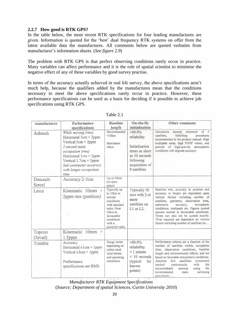
2.2.7 How good is RTK GPS?

In the table below, the most recent RTK specifications for four leading manufactures are

given. Information is quoted for the „best‟ dual frequency RTK systems on offer from the

latest available data the manufactures. All comments below are quoted verbatim from

manufacturer‟s information sheets. (See figure 2.9)

The problem with RTK GPS is that perfect observing conditions rarely occur in practice.

Many variables can affect performance and it is the role of spatial scientist to minimise the

negative effect of any of these variables by good survey practise.

In terms of the accuracy actually achieved in real life survey, the above specifications aren‟t

much help, because the qualifiers added by the manufactures mean that the conditions

necessary to meet the above specifications rarely occur in practice. However, these

performance specifications can be used as a basis for deciding if it possible to achieve job

specifications using RTK GPS.

Table 2.1

Manufacturer RTK Equipment Specifications

(Source; Department of spatial Sciences, Curtin University 2010)

21

2.3 Trimble GCS500 and 600 Grade Control System Cross Slope Control

2.3.1 GCS500 Grade Control System Cross Slope Control

The GCS500 Grade Control System is a cross-slope control system designed to be used on

motor graders for fine grading work. The system uses two AS400 angle sensors and one

RS400 rotational sensor to calculate the cross slope of the blade. The system lets the operator

select which side of the blade is controlled, and switch sides on the return pass. The highly

flexible AS400 has 100% slope capability, making the system ideal for a wide range of

applications, including cutting road slopes, ditches and embankments.

The software with a powerful range of features specifically designed for cross-slope and

blade elevation on motor graders will be provided when using CB420 Control Box with the

combination of GC500. The GCS500 can be upgraded to a GCS600 for cross-slope elevation

control. The applications for GCS500 are for the Road Maintenance, Road Construction,

Sports Fields, Embankments, and Road Ditches. (Trimble, 2010).

2.3.2 GCS600 Grade Control System Cross-Slope and Elevation Control

The GCS600 Grade Control System is a highly flexible, cross slope and elevation control

system designed to be used on motor graders for fine grading work. The GCS600 uses two

AS400 angle sensors and one RS400 rotational sensor to calculate the cross slope of either

side of the blade, as well as an LR410 Laser receiver and ST400 Sonic Tracer to provide

elevation control. Using the ST300, the system allows stringline, previous pass, or curb and

gutter tracing. Using one or two LR410 laser receivers, you can use the system for fine

grading plane surfaces. The GCS600 system is ideal for applications with tight tolerances and

finished grade work. The application for GCS600 are for the; Small-to-Large Housing and

Building Site Pads, Road Construction, Highway Construction and Maintenance, Runways,

Embankments and road ditches (Trimble, 2010).

2.3.2.1 Trimble ST400 Sonic Tracer

The Trimble ST400 Sonic Tracer uses ultra sonic signals to maintain a set distance or

elevation from an object, a design surface, or the ground.

When mounted to a motor grader or dozer blade, the ST400 can be used to reference a string

line, curb and gutter, or previous pass as a grade control reference.

The Trimble ST400 Sonic Tracer offers heavy and highway contractors:

Multicolored integrated grade display - conveys clear grade feedback to the

machine operator for higher productivity

Selectable sensor accuracy - provides typical accuracy of +/- 1mm (0.04") to control

elevation for even the tightest jobsite specifications

The ST400 Sonic Tracer can be used in single or dual configuration and is compatible with

Trimble GCS300, GCS400, GCS600, and GCS900 Control Systems.

22

Figure 2.10, (Trimble, 2010)

2.4 Leica TPS 1200

2.4.1 Introduction Leica TPS 1200 total stations are built up for speed, accuracy, ease to

use and reliability. It‟s better and more efficiently than ever before and they combine

perfectly with GPS and the position can be calculated in the real time.

TPS and GPS have the same operation and they are very user friendly. They have similar

format and data management systems, and cards can be transferred from one to the other and

work in the same way. It‟s also accommodated with software package for visualization,

conversions, quality control, processing, adjustment, reporting and export.

2:4:2 Power search (PS)

Power Search used during complete loss of lock due to obstructions; fast rotating laser fan

finds reflector quickly and ATR fine Points. In lock mode TPS 1200 remains locked onto the

reflector and follow it as it moves. Measurements can be taken at any time and, as software

predicts reflector movements, TPS 1200 continues to track inspite of obstructions and short

interruptions. (Source: Leica Geosystems, 2010)

Table 2.2; PS specifications (Source: Leica Geosystems, 2010)

23

2:4:3 Angles

The TPS 1200‟s angle measurement system consists of a static line-coded glass circle, which

is ready by a linear CCD array. A special algorithm is then used to determine the exact

position of the code lines on the array and thus determine the precise angle measurement.

Angle measurement system operates continuously providing instant horizontal and vertical

circle readings that are automatically connected for any “out of level” by a centrally located

twin axis or dual axis compensator.

The compensator consists of an illuminated the pattern on a prism, which reflected twice by a

liquid mirror. These form the reference horizon. The reflected image of this line pattern is

read by a linear CCD array and then used to mathematically determine both of the tilt

components. These calculated tilt components are the used to correct all angle measurements

in real time.

Table 2.3 TPS 1200 Series angle Accuracies (STD Dev)

TPS 1201 TPS 1202 TPS 1203 TPS 1205

Accuracy(Std dev)

Hz, V: 1‟‟ 2‟‟ 3‟‟ 5‟‟

Display resolution 0.1‟‟ 0.1‟‟ 0.1‟‟ 0.1‟‟

Method Absolute, continuous.

Compensator

Working Range: 4‟ 4‟ „4‟ 4‟

Setting Accuracy: 0.5‟‟ 0.5‟‟ 1.0‟‟ 1.5‟‟

2.4.4 Distance measurement.

TPS 1200 has three measuring modes which are:

1. Infrared laser measurement mode IR

2. Visible red laser measurement mode RL

3. Long range visible red laser measurement mode LO

The TPS 1200 series utilizes a phase shift measurement technique (EDM), which operates in

both the reflector and reflectorless modes.

The EDM works by transmitting an invisible bean (100 MHZ modulated frequency), the

beam is then reflected back by the target or prism. Photo receiver and converted into an

electrical signal. Once this electrical signal is digitized and accumulated, the distance is then

determined via standard phase measurement techniques.

24

Table 2.4 TPS Distance measurements with (IR mode) prisms-reflectors.

EDM measuring

program

Standard deviation

Standard prism

Standard deviation

Tape(targets)

Measurement

Time, typical [s]

Standard 2mm + 2ppm 5mm + 2ppm 1.5

Fast 5mm + 2ppm 5mm + 2ppm 2‟‟ 0.8

Tracking 5mm + 2ppm 5mm + 2ppm <0.8

Averaging 2mm + 2ppm 5mm + 2ppm -

(Source: Leica Geosystems, 2010)

During the measurements, there may be beam interruptions, severe heat shimmer and moving

objects within the beam path can result in deviations of the specified accuracy. The display

resolution is 0.1mm.

2.4.5 ATR

Leica refers ATR as “Automatic Target Recognition” ATR/LOCK. It actively follows the

prism as it moves and automatic fine pointing to prism.

The accuracy with which the position of the prism can be determined with automatic Target

Recognition (ATR) depends on several factors such as internal ATR accuracy, instrument

angle accuracy, prism type, selected EDM measuring program and external measuring

conditions. The ATR has a basic standard deviation level of + 2mm. Above a certain

distance, the instrument angle accuracy predominates and takes over the standard deviation of

the ATR.

The following graph shows the ATR standard deviation based on two different prism types

distance and instrument accuracies.

Table 2.5; (Source: Leica Geosystems, 2010)

LEICA ATR Specifications

25

Table 2.6; (Source: Leica Geosystems, 2010)

2.4.6 Servo Drive.

The TPS1200 is driven by servomotors mechanically. These servomotors‟ are used to rotate

both horizontal and vertical axis. The downside of these motors is that they use a lot more

power than Mag Drive technology and they are only able to rotate at a fraction of the speeds.

2.5 Trimble 5600 (ATS) Total station

2.5.1 ATS (Advanced Tracking Sensor)

The Trimble ATS is a dual mode instrument founded on Geodimeter technology, which

allows increasing productivity on site.

Automatically lock on the active target and continuously measures the target‟s position and

transmits the data to the computer, which then determines the desired elevation and slope for

that position (Trimble Data sheet, 2004).

The Trimble ATS starts with the foundation of the Trimble 5600 Total Stations and has

enhanced features for high performance automatic machine tracking. In advanced tracking

mode for machine tracking. In advanced tracking mode for machine control, the ATS

combines with on machine controllers and operator display to guide and control machinery

and vessels performing construction tasks- without need for stakes in the ground. The ATS

also drives a machine control system, which allows an operator to work single handed with

all design and cut/full information right in the cab.

It‟s designed specifically for the high speed, low latency demands of machine control; the

ATS in Advance tracking made has a latency of less than 200 Kms and selectable output rate

between 1 and 6HZ. Angle and distance data from the instrument are synchronized, providing

26

a machine with precise, up to date information, increasing the accuracy and speed at which a

machine works.

This low level of latency combined with the instruments turning speed enable the ATS to

track a machine driving as close as 30m at a speed of 46 kph without losing a lock (Trimble

2010)

The instrument has built in search intelligence to locate the target if contact is temporarily

interrupted by, for example, a passing vehicle. The programmable target recognition

capability of ATS allows operation of several Instruments on the same site without signal

interference. It can recognize one out of active targets, providing freedom to operate four

machines or surveys in the same part of the construction site without radio or reflective

surface interference. (Trimble 2010)

As a part of the Blade pro ® 3D grade control system, the Trimble ATS robotic total Station

provides precise vertical positioning – accurate to ± 5 mm making it ideal for finished grade

work. The system also gives the machine operator full control over the earth works on a site.

It was display screen in the machine cab that shows the exact 3d position of the blade in

relation to the design at the time.

In addition, value sensors can be added for fully automatic machine control. The slope and

elevation of the blade are therefore controlled by the system, not by the machine operator

reducing errors and avoiding expensive re-work.

2.5.2 Synchronization of data from angle and distance measurements sensors means that

the output data is computed for a single instantaneous location of the moving machines

compared with the standard total station instruments that are optimized for static prism

measurement. This results in higher 3D position accuracy for dynamic measurements or

machine tracking applications. (Source; Trimble 2010).

Figure 2.11, Synchronization; (Source: Trimble, 2010)

27

2.5.3 Latency

The precise position of the machine at any given times is dependent on the age or latency of

the positioning data received. If the age of the data is small and specific, the on board

application software can compensate for the errors associated with the data age giving a more

accurate location of the machine in real time.

Figure 2.12; (Source: (Source: Trimble, 2010)

2.5.4 Servo controls.

The Trimble 5600 series Instruments are equipped with servo controlled motors for

positioning of the unit. The servo is in use when performing a number of different operations,

when turning the motion knobs, when positioning with the servo control keys, for automatic

test and calibration or when using the tracker robotic surveying.

Trimble 5600 series (servo) instrument is equipment with an optional Tracker unit which can

perform Surveying tasks using the Auto lock function, and if the instrument is upgraded with

a radio, a spatial scientist will be able to perform Robot Surveying in conjunctions with

RMT.

2.5.5 RMT Super Multi Channel consists of a prism ring with seven 1‟‟ prisms and an

RMT with a set of active diodes forming a full 360 degree circle. It can be used for distance

up to 1000m. The RMT can be set to four different target channel IDs. The RMT SUPER

Multi channel has been developed for dynamic operation with the Trimble ATS Instruments.

28

Figure 2.13, RMT ATS Multi Channel; (Source: Leica Geosystems, 2010)

The RMT ATS multi channel is designed for operation at distances up to 1000 m (700m in

Robotic and ATS Modes). In dynamic operation at distances less than 3m, signal to distance

meter may be lost depending on the rotation of the prism ring in relation to the instrument. At

distance 3m up to 8m there may be an error in slope distance of up to 15mm at 3m and

decreasing as the distance increases.

2.5.6 Distance meter Calibration.

In order to achieve as high accuracy as possible the distance meter should be calibrated

regularly by application software. These distance meter will be seen as loss of signal for up to

two seconds.

2.5.7 Auto-Search

The Trimble ATS has built in automatic search capability that is activated automatically if the

signal is lost when the system is running in machine control mode. This system has to be

activated by the application software in order to work as intended. If the auto search is active

then it will search for the target. When the target is lost the system will search within the

search sector (window) with a number of horizontal scans at the vertical angle where the

signal was lost. The number of scans is set to five by default but the application software may

exclude them or set any number of scans up to 50 or maximum two minutes.

29

If the target is not found during these horizontal scans then a spiral search will start controlled

by software application. If no target is found then the Trimble ATS will return to the position

where the signal was lost and report to the application software that no target was found.

2.5.8 Distance

The distance module of Trimble 5600 series operates within the infrared area of the

electromagnetic spectrum. It transmits an infrared light beam. The reflected high beam is

received by the instrument and, with the help of a comparator, the phase delay between

transmitted a received signal is measured. The time measurement of the phase delay is

converted and displayed a distance with the mm accuracy.

2.5.9 Angle measurement System.

The Trimble 5600s meets all demands for efficient and accurate angle measurement. The

angle method gives a full compensation for the following:

● Automatic correction for angle sensor errors.

● Automatic correction for collimation error and Trunion Axis Tilt.

● Automatic correction for tracker collimation error.

● Arithmetic averaging for elimination of pointing errors.

The electronic angle measurement system, which eliminates the angle errors that normally

occur in conventional theodolites. The principal of measurement based on reading an

integrated signal over the whole surface of the angle sensor and producing a mean angular

value. In this way, inaccuracies due to eccentricity and graduation are eliminated.

2.5.10 Dual Axis Compensator

The instrument is also equipped with a dual axis compensator which will automatically

correct both horizontal and vertical angles for any deviations in the plumb line. The system

warns immediately of any deviation in excess of ± 10 c (6‟).

2.5.11 Collimation Errors

Horizontal and vertical collimation of the instrument can be quickly measured and stored by

carrying out a simple pre-measurement test procedure. All angles measured thereafter are

automatically corrected. These collimation correction factors remain in the internal memory

until they are measured again.

2.5.12 Trunion axis Tilt

It is also possible to measure and store angular imperfections of the horizontal tilt axis

relative to the horizontal axis during the same pre-measurement test procedure. These tests

are usual carried:

Immediately prior to high precision angle measurement.

After transport where hard handling may have occurred.

When temperature differs by >10C from the previous application

30

2.6 Previous Tests Undertaken

There has been a very little testing besides the manufactures testing (specifications) in

relation to the dynamic accuracy of ATS, RTS and RTK GPS latencies.

Some previous tests carried out in order to „„determine the dynamic accuracy and reliability

of RTSs” were carried out by:

● Ceryova in 2002

● Chua in 2004, and

● Dennis Garget 2005

Other testing for RTK GPS latency were done and described in the following pages.

2.6.1 – Chua 2004.

Chua used the Trimble 5603 to perform the following testing:

Simple testing of a fixed circular path with various speeds. He used a bar with a known radius

and the distance between the RTS and pillar was fixed. The bar (prism) was then rotated in a

circular path at a very low speed whilst the RTS stored dynamic measurements directly to a

PC.

Straight line testing: He set up a prism on a fixed bench and moved the prism horizontally

along the bench. Using a CAD package, he determined that would be necessary to smooth his

results using the Kalman Filter. He then used the filtered results to produce final outputs

which he then used to draw his conclusion.

He concluded that; the reliability of RTS is greatly related to the speeds of the prism and

measurement distances (Chua, 2004). Furthermore, Chua elaborated that the dynamic

accuracy of an RTS is better at longer distances than at shorter distances.

He also attributes much of the results deviation to the shape of the prism, and that the tracked

reflected reading is not always a true indication of the centre of prism. This consequently

results in point positioning errors.

2.6.2 Ceryova 2002

Ceryova performed two separate tests similar to Chua except he utilized several different

types of RTS in order to obtain his result. The instruments used were Leica TCA 1800, Leica

TCRA 1101, and Zeiss Elta s10.

Fixed circular path test: He used a simulator for testing sensors of the circular path

measurement systems. The main arm would rotate in a horizontal plane and at the end of the

arm was a fixed measuring board that would rotate in the opposite direction to the spinning

arm. Measurement board and prism were always facing the observer. The platform was

31

rotated through a 0.5m radius at several speeds. The resulting measurements were then stored

to a pc.

Straight line test: He incised a line with an accuracy of o.1mm) into the middle of the metal

block. They then observed measurements from three separate stations all with different

relationships to this line (i.e. distance and angle)

He concluded that, as the speed of rotation increased the subsequent point deviation also

increased. He suggested that „„measurement of the cinematic target is influenced by a certain

systematic influence which is probably a result of the time slide between angular and length

measurement‟‟

Ceryora also went further and suggest that by increasing the speed of rotation you are also

increasing the mean error in the RTS automated pointing system.

2.6.3 Dennis Garget.

Garget performed tow similar tests which was previously done by Chua and Ceryova the only

difference is that, he extended the straight line for various speeds testing.

1. Fixed circular path testing at various speeds.

2. Extended straight line testing at various speeds.

This testing was performed at several target distance and at several target speeds.

2.6.4 Conclusion.

There are some distinct similarities between the results obtained by Chua, Ceryova and

Garget was all parties concluded that the overall accuracy of an RTS is dependent on two

main factors:

1. The speed of moving target: and

2. the distance from the RTS to the target. They also concluded that, the dynamic

accuracy of an RTS is improved as the target distance is increased.

They also concluded that, the dynamic accuracy of an RTS is improved as the target distance

is increased.

Furthermore, Garget concluded that both the accuracy and reliability of a given instrument is

further influenced by the speed at which an instrument is capable of reading distance

measurements. This is evident by the fact that the Leica instrument is far more accurate and

reliable than the Trimble instrument. This can be attributed to the fact that the Leica

instrument is quoted to read distance in generally <0.15 seconds, this opposed to the Trimble

instrument which is quoted to read distance in around 0.4 seconds. This significant difference

in distance measurement time increases the point latency present within the instrument quite

significantly. As a result the Trimble is far less accurate and reliable when compared to the

Leica(Garget, 2005)

32

2.7 RTK GPS latency in Dynamic Environment

The use of machine guidance is becoming so popular in small and large civil

construction sites. Latency is one of the primary factors presently affecting the suitability of

the AMG. In order to achieve the specific requirement of the AMG, the user‟s operators have

a requirement to know how responsive the guidance system is to changes in their spatial

location on the work site.

Latency in general may be defined simply as a measure of temporal delay

(MM Internet, 1999); or

(latency is the ) “Time taken to deliver a packet (of data) from the source to

the receiver. Includes propagation delay (the time taken for the electrical or

optical signals to travel the distance between the two points) and processing

delay” (Interoute,2005)

(Raymond,2005) defines latency as the delay between the time of fix and when

it is available to the use” Hence if the GPS is in motion, the platform on which

the measurements are being made will move some distance during the time

when the measurement is made and the time when it is available to the user.

Latency may be divided into two component described as internal processing latency and

transmission latency.

Internal latency is that quantity of time which the instrument takes to complete its internal

processes and present the data ready for use or transmission. Transmission latency is the

period of time to send the measurement data from the originating source to the user, in the

field (Bouvet et al, 2000)

Given that position error due to latency is a function of the update rate (total latency) and

velocity of the vehicle (Campbell, Carney and Kantowitz, 1998), then for any given latency

period, the dynamic platform position error will increase in a proportion with the platform

speed.

The following relates to hydrographic measurements (sounding equipments as an external

sensor) using GPS. Time lag latency can be experienced between when a sensor record is

measured and when it is recorded by the software. Similarly, a time lag (Latency) may be

experienced between when a GPS position is measured and when is recorded.

Most importantly, these two time lags may not be the same, and consequently the GPS

logged position may not be exactly the same location as the depth sensor when the

hydrographic data is logged. (Gibbings and O’Dempsey, 2005).

Previous studies to investigate the effects of latency in GPS measurements have been

completed. (Smith and Thomson,2003) outlined a method to evaluate GPS position latency in

the guidance system of an agricultural aircraft. The method involved reflecting a beam of sun

light vertically from the ground using two mirrors.

33

A photo–detector circuit under the wing triggered an extra data record to be inserted into the

GPS data log. This position could then be compared with the known position of the light

beam to determine position latency.

The resulting latency determination of less than 9 metres for all runs of testing. The error is

relatively small if you compare with an aircraft was travelling at 58 meters per second

(around 208.8km/h). The authors also report a high level of consistency in their findings,

stating that the differences in consecutive runs were all less than 0.7 meters (7.77℅ of the

error distance due to latency). The use of an optional sensor is seen as a very accurate means

of referencing the dynamic measurements back to the fixed frame of reference and has

therefore been adopted for this research project also.

2.8 Trimble ATS Evolution.

In early 1995, the first tests were performed for a machine control operation using a standard

optical robotic total operation Geodimeter 4400. Immediate test results indicate that, for

kinetic operations compared to standard surveying applications, the instrument had to

improve the way it measured and sent data to the control computer. Specifically, higher

output rate of measurement and synchronized angle and distance reading were required.

Standard total stations are optimized for static prism measurement; in contrast,

synchronization of data from the angle and distance measurement sensors allows output data

to be computed for a single instantaneous location of the moving machine. This results in

higher 3D position accuracy for dynamic measurements or machine tracking application.

Synchronization is a measure of how closely together in time the various polar coordinated

that form the data pocket are measured. If the data is not synchronized, the sensor gives an

incorrect position. The size of the error depends on how far apart in time the various

components (angle and slope distance) are measured, and the speed and direction of the

moving target.

Low latency for complete transmission the precise position of the machine at any given time

depends on the age or latency of the positioning data received, if the age of the data is recent

and specific.

2.8.2 3D Positioning Accuracy.

Total 3D positioning 3D positioning accuracy for the system is less than 2mm at 200mm. The

superior accuracy is based on the high accuracy specifications of a motorized, self tracking

and prism that follows the total station with an extremely precise angle reading system,

accurate in both. Horizontal and vertical to 1 arc second (o.3 mgon). Additionally, the

distance measured provides an accuracy of ±2 mm + 14ppm.

34

CHAPTER 3

RESEARCH APPROACH AND METHODOLOGY

3.1 Introduction

As previous described, the aim of this project is to test the accuracy and reliability of machine

Guidance when used in road construction. In order to achieve the objectives associated with

fulfilling this aim the following steps will need to be performed.

Field – Testing:

Creating the computer modal and give to the grader operator and start trimming on section of

the road of approximately 200-300m. Two layers will be tested and each layer had an

independent check following the approximately 50m intervals observed and checked by the

operator reading on his onboard screen and the surveyor by using a Leica Total station. The

testing procedure will also be explained in the following chapters.

The grader operator will be laying his blade on the ground on top of a piece of timber, he/

she will be checking the level by reading on the screen and will be recorded manual, at the

same time the surveyor will be holding on the same position and the results will be recorded

directly to the internal memory. The raw data will later be exported to the card and then to the

pc. The observation will be observed in static motion and this will be done after the job of

grading has been finished. This will be tested in according to manufacturer‟s specification.

Final check layers will be tested by a Total station TPS 1200 for comparison.

Data Analysis:

● Comparisons between my test and manufactures specifications.

● Comprehensive analysis of the test results.

As described by the literature review in chapter 2, previous testing performed by Ceryova,

Chua and Garget was based on testing the dynamic accuracy and the reliability of the robotic

total stations. Also Gibbings, O‟Dempsey, Raymond, Smith and others did a tremendous

work in testing the RTK GPS Latency in dynamic environment. There isn‟t many testing

measures has been done in the past in regards to the machine guidance, this will be a

challenge and I think, based on the ideas and examples described on chapter 2, the successful

results will be obtained.

35

3.2 Data collection and testing.

3.2.1 - Equipment used.

Three Instruments have been utilized throughout this project.

● Leica TPS 1202.

● Trimble 5600 ATS.

● Trimble GCS600 Grade Control System.

3.2.2 Main components of the instruments:

Leica – Robotic Total Station (Itself) within internal radio.

(1) 360 Prism (target); and

(2) Detachable/Remote keypad.

Trimble 5600 ATS (itself) with internal radio

(1) Grader

(2) 360◦ Trimble prism mounted directly above one side of the blade.

3.2.3 Trimble GCS600 Grade Control System

(1) Grader

(2) GPS Base on site.

(3) GPS antenna mounted directly above one side of the blade. The

GPS Antenna is connected together with Laser receiver underneath and transmitter located on

fixed point (within 1500). A Trimble GCS600 unit was utilized for this testing.

3.3 Project Planning.

They are several stages have been implemented in order to undertake this project:

1. Primary research, initial stage which involves background research and literature reviews

form magazines articles, books and journals. Previous tested accuracy and reliability.

2. Data collection and Testing. It involves collecting data in the field from Leica instrument

after the job being performed by Trimble ATS and Trimble GPS-AMG. The comparison of

Leica 1202 will give us an idea of the accuracy.

3. Analysis. The data collected and tested during stage two of this process will be edited,

plotted, reviewed and reports produced using 12d software. The reports will be printed in

plans and graphical form.

4. Discussion and comparison of the system: Plans, graphs and reports are to be analysed,

critical thinking and subsequent use in the entire project.

36

5. Conclusion: The data which has been analysed have to reflect the manufacturer‟s

specifications and draw conclusion to the various factors upon the accuracy and reliability of

the machines guidance systems.

3.4 Literature Contribution to Research Method

The literature review as described on chapter two has given me a basis of understanding the

RTS, ATS and RTK GPS so as to achieve the best possible results. Consideration must be

taken following the important aspects mentioned below:

(a) According to the manufacturer‟s specifications, each instrument has a different

distance measurement, speed and accuracy for RTS, ATS and RTK GPSs satellites

coverage.

(b) Rotation ability of different instrument is not the same. The RTS maintain a high

accuracy only in the length measurement (Ceryova et al, 2002).

(c) Accuracy of the results are closely associated with the speeds of the moving target

(Ceryova et al., 2002);

(d) Shorter observation ranges have larger standard deviation compared larger distances

(Retscher, 2002)

(e) Circular path testing straight line testing are the key components in determining the

dynamic accuracy of the RTSs (Kopacik, 1998).

(f) Measurements are not always taken to the centre of the target; this is caused by the

shape of the target (Chua, 2004).

3.5 Field Testing.

There were some tests undertaken for fixed circular extended straight line tests and latency on

GPS RTK as described on chapter 2.

To determine the fixed path, straight lines and latency associated with the above testing

equipments the measurements have been made in a dynamic sense. A detailed description of

this method is given in chapter 4 although a brief introduction to the testing method is

provided below.

37

Figure 3.1 Showing a plan view of the road at Gateway Project

The testing regime for this projects requires a section of road way. Chainage 12000 to 12280

was selected for this project (see a view plan above). The signal from the antenna is corrected

by whichever means is been used, when the operator initialize the GPS RTK on his onboard

screen. The fixed points provide a static reference and position data is recoded in conjunction

with the model supplied for travel in each direction past the fixed points at a range of

consistent speeds. By comparing the measured location with the known fixed position the

latency of the system can be calculated.

The testing is conducted over a range of speeds to better determine the relationship between

dynamic platform speed\ and latency error. These can be related to the example given by

Raymond 2005 as described on page 32 chapter 2.7

On ATS and RTS the testing will be conducted as descried on survey operations. During the

check up and pickup survey using a Leica RTS 1202 and cutting and fill operation using ATS

5600, these instruments have a similar operation of a moving targets during a survey

operation as described by (Garget, 2005) during his fixed circular path test. The target 360

38

Leica and 360 Trimble RTS were used for test in accordance to the manufacturer‟s

specifications. All this tests were carried during the day time.

3.6 Operation of RTS (leica1200), ATS (5600s) and RTK GPS

3.6.1 RTK GPS and Machine Controls that can assist in construction accuracies and

efficiencies. The GPS receiver on earth can “triangulate” its position from a minimum

number of 4 satellites. However, the standalone accuracy of any GPS receiver is only about ±

15mm. In this case, at least more than 5 satellites and by using a radio to broadcast

corrections from the base station to other rovers, and accuracy increases to 10mm.

The construction site where the testing has occurred has at least 3 base stations which are

adequate enough to achieve the requirements of the Main roads. According to the company

policies, they have decided to use the GPS grader when they are doing a rough grading (such

as Subgrade layer) and for the excavation purposes.

An RTK base station was set (fixed) near the test site to allow for the RTK correction

information to be obtained. The methodology designed in this research utilizes Trimble GPS

equipments only and no other testing is done using other GPS receivers from other

manufactures.

3.6.2 Operating on GPS (AMG)

Project contractor provided control points (primary or secondary controls) and conventional

grade stakes at critical points such as, but not limited to all PCs, PTs and super elevation

points begin full super, half level plane inclined etc.

The contractor set to utilize (RTK) GPS where the tolerances are within 20mm. a Trimble

GCS 600 GPS unit was utilized for this testing. It features an antenna with built in GPS

receiver and RTK radio. The GCS 600 uses tow AS400 angle sensors and an RS400 rotation

sensor to calculate the cross slope of either side of the blade.

Similar to ATS 5600 processes, but with this is more to be done by the grader operator. The

processed data (DTM in the flash card) from the surveyor will be handed over to the grader

operator who will insert onto on board screen panel. The operator will start – initialize the

GPS system and set the layer he/she is working on. The operator will check the blade by

laying the blade on the piece of timber or stake, and the surveyor will double check the

timber by taking or holding the prism pole on top of it. The results must coincide with the

operator so that everybody is happy with the outcome.

Also, the surveyor may put some benchmarks with relevant RL‟s (Reduced Levels)

close to the working area where by the operator can reach his blade for check without any

problem. Since we were working on the subgrade layer level with GCS 600, hence there was

no requirement for the surveyor to do a random check because of the series of benchmarks

39

installed on site and good enough for the grader operator to check on. Finally, the surveyor

observed or picked up the asbuilt survey and ready for the asbuilt report.

3.6.2 Operation of an ATS5600 (Field)

The ATS5600 operates by creating a new job in the card at anytime prior the data collection.

Scale factor distance unit and coordinate system was set or changed onto the instrument. Pre-

surveyed datum‟s which were done by the surveyors on site was keyed in the instrument.

3.6.2.1 Setup the instrument. The instrument was set on the tripod and observes at least

three known point by resection (free station) normal surveying procedures. The large battery

connected to the instrument usually last longer up to three days when it‟s new. Radio was

connected and turned in conjunction with the grader.

After the instrument was turned on the survey controlled software on data logger was opened

and wait for radios to establish communication, which takes up to three minutes and the level

screen appears after everything goes well. The instruments calibrate itself and rotates two

times and it beeps.

ACTIVE 360 TRACKER and TARGET INDICATION using a special designed prism called

„‟Tracker Target 360 Multi channel‟‟. The Tracker target includes a combination of the set of

standard corner prism which allows distance measuring from 15m to the maximum range.

The active 360 Remote Target sends a special signal to the ATS tracker unit.

The ATS tracker is located below the optical scope of the instrument. The signal is detected

and tracked after the Trimble ATS Tracker automatically indicates its location. The Trimble

ATS Total stations checks the availability of both parts of the tracker target throughout the

complete operation and only tracks the combination of both parts. To ensure that only the

tracker target to the Trimble ATS is continually detected and monitored, the Target features a

channel setting function. Set the ATS total station using the controlling software and the

telemetric link of the specific indication channel.

After surveyors job being completed, i.e. preparing DTM (TIN) modal which would be

handed to the grader operator. The instrument and job operation will be ready to go. The

surveyor will ensure that, the grader operator is happy by checking his levels how they read

on the screen. Surveyors usually use a piece of timber laid on the ground where the operator

can reach his/her blade. The operator will lay a blade on top of the timber or stake and will

read on the screen some levels which will be confirmed by a surveyor. In this case, the

surveyor will set the second set of the instrument (Leica 1202) and ultimately the level which

read by the operators grader screen will be confirmed otherwise adjusted. This is a

traditionally way were most operators follow the same system.

40

Another way, the surveyor would place a couple of Benchmarks near the site on the firm

ground, or stakes were by the operator will reach his/her blade for checks. The levels must be

written clearly on the Benchmarks or stakes. Say RL 10.000m. They also prefer to turn on the

modal and set the layers they are working on, and lay a blade on the road work in order to

compare with the surveyors numbers i.e. CUT/FILL 0.005m and both must read the same

numbers unless otherwise, or else the adjustments must be made. The checks between

operator and surveyor can be done in two to three occasions at different distances, say 10m

20 and 50m. After that the surveyor will not be required, only the machine will be working

and the credibility of the operator.

Walk talkies radios or mobile phones are used for communication between the surveyor and

the operator. The surveyor will be going to the field from time to time, just to check the

Trimble 5600 if it‟s still operating without troubles, flat batteries, and setup a Leica 1202 (for

quick or random) check the layer works if it correspond with the graders operation. If there is

a problem, then the job can be stopped for a while and attend the problem before more

damage occurs. One of the problems which is likely to occur are the instrument being

disturbed by windy, or wrong modal (DTM) or it wasn‟t checked properly, or the grader

operator reset the wrong layer and also a surveyor could contribute to errors or blunder.

Finally, after the whole section has been completed by machine guidance. The duty of spatial

scientist will be to pick up the asbuilts survey check and reporting.

3.7 Operation of a Leica 1202 (Field)

The Leica 1202 was utilized on this operation, and the purpose was to check and compare

with the ATS5600 and GCS 600 equipments.

After the instrument was setup by resection, the first step will be to check the control

benchmarks or existing levels from the benchmark. The reason of doing this is because of the

errors during the setup and also, we are dealing with position verticals (heights) and we need

to be perfect in order to achieve the pavement thickness.

Then the instrument was used during the checks with grader operator, random checks and

finally pickup surveys for asbuilt checks and reporting.

Conclusion

All the tests mentioned in this chapter have been completed successfully and the result will

be discussed in the next chapter.

41

Two instruments were used for testing the accuracies in the form of layers, and instrument

was used to check and record the data. It was difficult to use all the equipments as it was

described in the previous chapter, due to the time constraints.

Following the outcome of the result, the conclusion will be drawn and the recommendations

will be presented.

CHAPTER 4

DATA ANALYSIS AND DISSCUSSION

4.1 Introduction

The previous chapter fully described the method of measuring and how the latency could

occur during field operations. The methods were also providing comparisons between the

measurements observed by the leica1202 instrument with ATS5600 and GSC600.

This chapter is talking about analysis of the data used to obtain useful information resulting

from the information of the testing regime. The result will give a benchmark for this ongoing

research and discussion. It will also, be noted that the data analysis process for ATS5600 data

is exactly the same as GSC600 because they have an identical format and their corrections

are automatically applied before the data is recorded.

As it was described earlier, the RTS Leica is an addition unit required during checks

inspection and record keeping for this project. Majority of analysis is performed using

Microsoft excel spreadsheet program. The program statically analysis and evaluation of the

test result, then reports as shown on the chart below.

42

Figure 4.1; Analysis process

Raw data

Raw data Edited

Import raw data into 12d model 12d model Alignment

Import chainage and offset Produce chainage and offset

Report into Excel

Generate Graphs and Statistics

Draw conclusion and compare to

Manufacturers specifications

4.2 Data Analysis

4.2.1 Raw data collection and Transfer

The initial raw data collected was recorded in the internal memory of Leica 1202 using Leica

formats and code lists according to the Main roads standards. The instrument is capable of

storing atleast one thousand points or shots. Asbuilt survey (survey points) were taken in

chainages by estimating three meters counting in each layer at the exactly position. During

the field operation, the raw data captured was viewed and checked on site to see if whether

are sufficient and well captured, or there some missing points during operation. Leica1202

has a map screen used to check the captured points in real time by scrolling and zooming a

touch screen. All this is done to ensure the data captured is right.

The ATS data transfer and GSC 600 don‟t store any data although they are capable of. Leica

1202 instrument was used to store all the data in all different layers. The data was then

exported to the flash card (Internal memory to the card) using a special formatted files

designed for downloading or exporting data. Inside the flash card, there is a folder called

Data, the folder stores a reduced files in the form of radians or Easting, Northing, Reduced

Levels (RL) and point name or description format.

43

4.2.2 Data transfer to a personal computer

The data was then transferred to a PC for analysis. The Flash card was plugged into the PC

and imported data into 12d software using an ASCII import command. In 12d software, the

data could be seen and edited and changes could be made. Also the 12d software was used to

smooth the data and adjust them.

4.3 Software utilised and outputting data for analysis

Two main software packages below were utilised whilst undertaking the analysis of the test

data.

12d Software; and

Microsoft Excel spreadsheet

12d model received a raw data from the instrument and converted into a spatial format. This

spatial data was then used to produce, E, N chainage and offsets and final reporting. Since the

12d model had an electronic design given by the contractor, the job of obtaining the chainage

and offset was very easy. The 12d software was also doing the TIN (DTM) creation for the

grader operators.

In 12d format there is (file 1/0 –Data output-12da/4a data) facility enables to exchange and

backup complex string data in an open documented manner. 12d ASCII format caters 12d

Model string types including 2d, 3d, 4d, pipeline, roads alignment and super strings.

4.4 Analysing the Database information

The analysis of data is performed using the Microsoft Excel spreadsheet program. Raw data

relating to the measured positions (for both Trimble Total station and GPS was exported to

the 12d for processing before transferred to the Excel), and the example of extracted data

which produces the graph is shown below.

44

Table 4.1 showing an example of database information on spreadsheet.

Point Point Point Design

Chainage Offset Survey Design

Error (m) Design

12020.00 6.669 11.997 12.011 0.014 0

12029.75 6.342 11.877 11.887 0.01 0

12039.77 6.499 11.757 11.763 0.006 0

12049.48 6.068 11.603 11.614 0.011 0

12059.47 6.396 11.467 11.473 0.006 0

12069.3 6.097 11.314 11.305 -0.009 0

12079.38 6.759 11.145 11.149 0.004 0

12089.03 6.194 10.954 10.953 -0.001 0

12099.22 6.074 10.739 10.749 0.01 0

12108.32 6.087 10.55 10.561 0.011 0

12118.69 6.002 10.321 10.331 0.01 0

12127.66 6.147 10.14 10.136 -0.004 0

4.4.1 Analysing the GCS600 GPS

The latency of each run by machine GPS grader can be calculated from the raw position data.

Averages of the distance error can be computed for the run which are made at speed (i.e.

rejecting any outliers) Thus results in average latency distance errors for each run.

To ensure the distance over time is equal to speed. The calculation performed as each run at

each speed share a constant speed. If the majority are at the same speed but one run pair is

significantly different, then the run should be omitted from calculation of average latency for

that speed range. Higher speed observations will show a larger distance error due to latency,

and if the outlying machine run is included, it will distort the average latency computed for

that speed.

The previous pages defined the latency as the “delay between the time of fix and when it‟s

available to the user”. If the GPS is in motion, the platform on which the measured values are

being made will move some distance during the time when it is available to the user.

During the testing regime, they were some selected positions with an interval of 50m. Each

point were tested by the GPS and ATS onboard machine by laying the blade on the ground

and checked by a surveyor (me) with Leica Total station (see Table 4.4), and all this were

done after a very good setup, initialisation for all equipments and the comparisons were made

on site between the grader operator and Surveyor. In general the overall results are shown on

tables (4.8 and 4.9).

45

Table 4.2 showing analysis of data for Trimble GCS600, captured by leica instrument and

compared with levels from machine operator’s readings

GCS600 GPS data

----------------------------------------------------------------

Point Point Point Point Design Point

Desc Chainage Offset Level Level Conformance

UCE 12000.016 13.698 12.015 12.021 -0.006

UCE 12057.920 13.998 11.345 11.326 0.019

UCE 12047.626 14.323 11.512 11.489 0.024

UCE 12097.197 13.970 10.637 10.627 0.010

UCE 12146.973 13.849 9.563 9.537 0.026 > 0.025 ( 0.001)

UCE 12197.815 13.721 8.418 8.403 0.015

UCE 12236.665 13.636 7.547 7.536 0.011

Table 4.3 showing readings from GPS machine operator booked manual in stop and go

motion by laying the blade on the UCE layer after the final trimming.

----------------------------------------------------------------



UCE 12000.016 13.698 12.018 12.021 -0.003

UCE 12057.920 13.998 11.339 11.326 0.013

UCE 12047.626 14.323 11.513 11.489 0.024

UCE 12097.197 13.970 10.637 10.627 0.010

UCE 12146.973 13.849 9.569 9.537 0.032

UCE 12197.815 13.721 8.417 8.403 0.014

UCE 12236.665 13.636 7.553 7.536 0.017

Table 4.4

COMPARISON OF DATA EXTRACTED FROM TABLE 4.2 and 4.3

CHAINAGE OFFSET

From CL

GPS

GRADER(onboard

operator‟s readings)

LEICA TOTAL

STATION

(surveyors

recording)

DIFFERENCE

Vertical Levels Vertical Levels Vertical Levels

12000.016 13.698 12.018 12.015 0.003

12057.920 13.998 11.345 11.339 0.006

12047.626 14.323 11.513 11.512 0.001

12097.197 13.970 10.637 10.637 0.000

12146.973 13.849 9.569 9.563 0.003

12197.815 13.721 8.417 8.418 -0.001

12236.665 13.636 7.553 7.547 0.006

46

4.4.2 Analysing the Trimble ATS5600

The trimble ATS total station were done in a similar fashion as explained in the previous sub

section. Also the interval of 50m were used to check the vertical levels. As described in an

earlier chapters, several softwares were utilised. Among those, 12d were used to remove and

smoother the observation results.

Outliers were taken into consideration during analysis of measured values. Those measured

values which could be analysed due to lose of lock or any other uncertainty of the ATS

grader were eliminated from further analysis. The test of this regime was similar to cirlcular

path test which were done by Chua and Garget. Having a Trimble ATS being setup

somwhere and the observation of the grader movement will obviously give the horizontal and

vertical results. Measurements were observed in various distances at different speeds.

The distance between the setup station and the moving grader was less than 200m of either

side of the road, and the higher speed of the ATS was used which tends not to loose the lock

quite easily. The operator will have a runs up and down until he achieves the results before he

calls the surveyor to check. The analysed results are shown on table -------- below.

Table 4.5 showing analysis of data for Trimble ATS5600, captured by leica instrument and

compared with levels from machine operator’s readings

Trimble ATS5600 data

----------------------------------------------------------------



CTB 12000.095 13.466 12.410 12.413 -0.003

CTB 12049.490 13.477 11.842 11.837 0.005

CTB 12098.919 13.526 10.992 10.979 0.014

CTB 12148.351 13.493 9.898 9.896 0.002

CTB 12197.979 13.515 8.798 8.792 0.006

CTB 12257.391 13.524 7.486 7.472 0.015

Table 4.6 showing readings from ATS machine operator booked manual in static motion by

laying the blade on the CTB layer after the final trimming.

Trimble ATS5600 data

----------------------------------------------------------------



CTB 12000.095 13.466 12.412 12.413 -0.001

CTB 12049.490 13.477 11.842 11.837 0.005

CTB 12098.919 13.526 10.994 10.979 0.015

CTB 12148.351 13.493 9.898 9.896 0.002

47

CTB 12197.979 13.515 8.798 8.792 0.006

CTB 12257.391 13.524 7.489 7.472 0.017

Table 4.7

COMPARISON OF DATA EXTRACTED FROM TABLE 4.5 and 4.6

CHAINAGE OFFSET

From CL

ATS5600

GRADER(onboard

operator‟s readings)

LEICA TOTAL

STATION

(surveyors

recording)

DIFFERENCE

Vertical Levels Vertical Levels Vertical Levels

12000.095 13.466 12.412 12.410 0.002

12049.490 13.477 11.842 11.842 0.000

12098.919 13.526 10.994 10.992 0.002

12148.351 13.493 9.898 9.898 0.000

12197.979 13.515 8.798 8.798 0.000

12257.391 13.524 7.489 7.486 0.003

4.4.3 Further Analysis for the Trimble ATS5600 and GPS grader

Furthermore, both layers were recorded by Leica Total station following the chainages and

offsets to clarify the analysis of results. The reports from table 4.4 and 4.7 show what has

been achieved on the pavement layers when using both equipments.

Table 4.8 Showing the analysis of data for Trimble GCS600 GPS

12D MODEL - SURVEY CONFORMANCE REPORT: PAVEMENT

File: Z2 UCE Ch 12000 to 12260.rpt

Page: 1

----------------------------------------------------------------

Original Survey File : Z2 UCE Ch 12000 to 12260 sk

Lot Number : Ch 12000 to 12260

Instrument : Trimble GPS GC600

Lot Description : UCE 710mm below Comformance check

Project : Gateway student

Control String : "Z2 M2AS GUP FLOG->FLOG"

Design Pavement Tin : "Z2 M2AS GUP FLOG dtm"

Depth From Design : 0.710 (vertical)

Tolerances Measured : vertical

Upper Tolerance : 0.025

Lower Tolerance : -0.025

----------------------------------------------------------------

48



----------------------------------------------------------------

UCE 11999.842 6.158 11.829 11.797 0.033 > 0.025 ( 0.008)

UCE 11999.939 7.969 11.858 11.850 0.007

UCE 12000.005 10.878 11.941 11.937 0.004

UCE 12000.016 13.698 12.015 12.021 -0.006

UCE 11999.965 15.322 12.085 12.070 0.014

UCE 11999.865 18.958 12.163 12.181 -0.018

UCE 11999.947 23.810 12.302 12.325 -0.024

UCE 12000.055 26.576 12.387 12.407 -0.020

UCE 12010.077 6.487 11.727 11.710 0.016

UCE 12009.986 8.900 11.817 11.784 0.033 > 0.025 ( 0.008)

UCE 12009.950 11.582 11.867 11.864 0.003

UCE 12009.840 13.749 11.945 11.931 0.014

UCE 12009.895 15.538 11.997 11.983 0.014

UCE 12009.832 19.020 12.068 12.089 -0.021

UCE 12009.840 23.462 12.234 12.222 0.012

UCE 12009.771 26.586 12.314 12.317 -0.002

UCE 12020.405 6.247 11.626 11.594 0.032 > 0.025 ( 0.007)

UCE 12020.903 9.327 11.715 11.680 0.035 > 0.025 ( 0.010)

UCE 12021.047 11.545 11.778 11.745 0.032 > 0.025 ( 0.007)

UCE 12019.051 15.156 11.855 11.876 -0.021

UCE 12019.344 18.739 11.962 11.980 -0.019

UCE 12019.524 23.802 12.117 12.130 -0.013

UCE 12019.841 26.676 12.200 12.213 -0.013

UCE 12027.262 6.323 11.534 11.516 0.018

UCE 12027.346 8.113 11.592 11.569 0.023

UCE 12027.312 11.177 11.683 11.661 0.021

UCE 12026.860 14.130 11.773 11.755 0.017

UCE 12026.999 15.647 11.821 11.799 0.021

UCE 12029.936 18.781 11.835 11.858 -0.023

UCE 12029.954 23.310 11.972 11.993 -0.022

UCE 12029.852 26.764 12.081 12.098 -0.017

UCE 12037.640 6.250 11.394 11.384 0.011

UCE 12037.717 8.298 11.461 11.444 0.017

UCE 12037.706 11.023 11.535 11.526 0.009

UCE 12037.607 13.674 11.623 11.607 0.017

UCE 12039.127 15.202 11.627 11.633 -0.006

UCE 12039.275 18.917 11.724 11.743 -0.019

UCE 12039.530 23.552 11.868 11.878 -0.010

----------------------------------------------------------------


File: Z2 CTB Ch 12000 to 12260 sk .rpt

Page: 2

49

----------------------------------------------------------------



----------------------------------------------------------------

UCE 12039.608 26.689 11.992 11.971 0.021

UCE 12048.037 6.004 11.253 11.233 0.019

UCE 12047.962 8.043 11.324 11.296 0.028 > 0.025 ( 0.003)

UCE 12047.842 10.754 11.391 11.379 0.013

UCE 12047.626 14.323 11.512 11.489 0.024

UCE 12050.272 15.384 11.473 11.482 -0.009

UCE 12050.276 18.721 11.560 11.582 -0.022

UCE 12050.236 23.437 11.722 11.724 -0.002

UCE 12050.120 26.510 11.803 11.818 -0.016

UCE 12058.084 5.802 11.100 11.077 0.022

UCE 12058.011 8.143 11.171 11.149 0.023

UCE 12057.976 10.938 11.257 11.233 0.024

UCE 12057.920 13.998 11.345 11.326 0.019

UCE 12058.800 15.423 11.352 11.355 -0.003

UCE 12059.308 19.568 11.448 11.471 -0.023

UCE 12059.309 23.930 11.604 11.602 0.003

UCE 12059.456 26.452 11.669 11.675 -0.006

UCE 12066.748 6.074 10.971 10.946 0.025

UCE 12066.673 8.376 11.043 11.017 0.026 > 0.025 ( 0.001)

UCE 12066.547 11.373 11.130 11.109 0.022

UCE 12066.384 14.292 11.218 11.199 0.019

UCE 12066.376 16.087 11.265 11.253 0.012

UCE 12069.556 19.172 11.284 11.292 -0.009

UCE 12069.576 22.927 11.390 11.405 -0.015

UCE 12069.383 26.269 11.492 11.508 -0.016

UCE 12076.496 6.125 10.804 10.781 0.022

UCE 12076.585 8.611 10.879 10.854 0.025

UCE 12076.578 11.181 10.941 10.932 0.010

UCE 12076.603 14.038 11.032 11.017 0.016

UCE 12076.570 16.146 11.093 11.081 0.012

UCE 12078.816 19.137 11.110 11.131 -0.021

UCE 12079.021 23.892 11.246 11.270 -0.024

UCE 12079.096 26.297 11.320 11.341 -0.021

UCE 12087.366 6.352 10.588 10.589 -0.001

UCE 12087.333 8.231 10.676 10.646 0.029 > 0.025 ( 0.004)

UCE 12087.209 10.919 10.751 10.729 0.021

UCE 12087.115 13.746 10.830 10.816 0.014

UCE 12087.076 16.210 10.902 10.891 0.011

UCE 12088.784 18.857 10.921 10.938 -0.017

50

UCE 12088.616 22.568 11.030 11.053 -0.023

UCE 12088.543 26.384 11.157 11.169 -0.012

UCE 12097.411 6.427 10.391 10.396 -0.005

UCE 12097.315 9.002 10.499 10.475 0.024

UCE 12097.250 11.595 10.564 10.554 0.010

UCE 12097.197 13.970 10.637 10.627 0.010

UCE 12097.156 16.186 10.690 10.694 -0.004

UCE 12098.797 19.084 10.728 10.749 -0.021

UCE 12098.838 23.363 10.864 10.876 -0.013

UCE 12098.854 26.348 10.979 10.965 0.014

----------------------------------------------------------------



Page: 3

----------------------------------------------------------------



----------------------------------------------------------------

UCE 12106.557 6.656 10.233 10.215 0.018

UCE 12106.545 8.729 10.296 10.277 0.019

UCE 12106.544 11.347 10.385 10.356 0.029 > 0.025 ( 0.004)

UCE 12106.543 13.771 10.456 10.428 0.028 > 0.025 ( 0.003)

UCE 12108.986 15.586 10.410 10.431 -0.021

UCE 12108.892 18.805 10.505 10.529 -0.025

UCE 12108.842 23.212 10.639 10.662 -0.023

UCE 12108.818 26.212 10.737 10.753 -0.016

UCE 12116.195 6.422 10.027 9.999 0.028 > 0.025 ( 0.003)

UCE 12116.373 8.764 10.069 10.065 0.004

UCE 12116.378 11.566 10.169 10.149 0.020

UCE 12116.362 14.477 10.262 10.237 0.025

UCE 12118.432 15.508 10.203 10.222 -0.019

UCE 12118.683 19.095 10.310 10.323 -0.013

UCE 12118.818 23.222 10.450 10.444 0.006

UCE 12118.756 26.168 10.552 10.534 0.018

UCE 12126.769 6.402 9.790 9.763 0.026 > 0.025 ( 0.001)

UCE 12126.715 8.059 9.835 9.814 0.021

UCE 12126.719 10.884 9.906 9.899 0.007

UCE 12126.737 13.840 10.012 9.987 0.025

UCE 12129.312 15.514 9.960 9.980 -0.020

UCE 12129.256 18.842 10.078 10.081 -0.003

UCE 12129.005 22.870 10.220 10.207 0.013

UCE 12128.815 26.241 10.319 10.312 0.006

51

UCE 12137.033 6.136 9.552 9.527 0.025

UCE 12137.049 8.503 9.622 9.598 0.024

UCE 12136.839 11.238 9.703 9.684 0.019

UCE 12136.773 14.048 9.789 9.770 0.019

UCE 12136.766 16.020 9.854 9.829 0.024

UCE 12138.288 19.081 9.872 9.888 -0.016

UCE 12138.427 23.288 10.022 10.011 0.011

UCE 12138.567 26.213 10.112 10.095 0.018

UCE 12147.081 6.135 9.332 9.304 0.028 > 0.025 ( 0.003)

UCE 12147.086 8.208 9.389 9.366 0.023

UCE 12147.012 11.200 9.474 9.457 0.017

UCE 12146.973 13.849 9.563 9.537 0.026 > 0.025 ( 0.001)

UCE 12146.996 16.088 9.616 9.604 0.012

UCE 12148.351 18.801 9.634 9.655 -0.021

UCE 12148.351 23.092 9.779 9.784 -0.005

UCE 12148.289 26.386 9.863 9.885 -0.022

UCE 12157.162 6.441 9.110 9.089 0.021

UCE 12157.294 9.370 9.194 9.173 0.020

UCE 12157.279 11.518 9.255 9.238 0.017

UCE 12157.168 14.088 9.341 9.318 0.024

UCE 12157.128 15.970 9.397 9.375 0.021

UCE 12158.134 19.697 9.440 9.465 -0.025

UCE 12158.356 23.890 9.560 9.585 -0.025

UCE 12158.325 26.423 9.638 9.661 -0.023

----------------------------------------------------------------



Page: 4

----------------------------------------------------------------



----------------------------------------------------------------

UCE 12167.588 6.638 8.865 8.863 0.003

UCE 12167.528 8.969 8.942 8.934 0.008

UCE 12167.399 11.302 9.026 9.007 0.020

UCE 12167.332 13.594 9.098 9.077 0.021

UCE 12167.381 15.928 9.156 9.146 0.010

UCE 12168.226 18.254 9.174 9.196 -0.022

UCE 12168.276 22.430 9.296 9.320 -0.024

UCE 12168.120 26.290 9.423 9.441 -0.018

UCE 12177.302 6.379 8.657 8.639 0.018

UCE 12177.550 8.782 8.700 8.705 -0.005

UCE 12177.771 11.405 8.784 8.779 0.005

UCE 12177.773 13.861 8.878 8.853 0.025

52

UCE 12177.820 15.798 8.933 8.910 0.023

UCE 12177.958 18.941 8.978 9.001 -0.023

UCE 12178.065 23.125 9.100 9.123 -0.024

UCE 12178.117 26.332 9.203 9.218 -0.015

UCE 12187.804 6.229 8.427 8.401 0.026 > 0.025 ( 0.001)

UCE 12187.756 8.580 8.500 8.472 0.028 > 0.025 ( 0.003)

UCE 12187.685 10.695 8.558 8.537 0.020

UCE 12187.556 13.493 8.651 8.624 0.027 > 0.025 ( 0.002)

UCE 12187.555 15.186 8.651 8.675 -0.024

UCE 12187.509 17.884 8.736 8.757 -0.021

UCE 12187.760 22.471 8.866 8.889 -0.023

UCE 12187.925 26.210 8.980 8.997 -0.017

UCE 12197.860 6.334 8.203 8.180 0.023

UCE 12197.788 8.663 8.261 8.252 0.009

UCE 12197.811 11.160 8.338 8.326 0.011

UCE 12197.815 13.721 8.418 8.403 0.015

UCE 12197.772 15.580 8.465 8.460 0.006

UCE 12198.024 19.433 8.554 8.569 -0.015

UCE 12197.962 23.321 8.671 8.687 -0.016

UCE 12197.952 26.115 8.748 8.771 -0.022

UCE 12207.368 6.314 7.976 7.968 0.008

UCE 12207.345 8.245 8.049 8.027 0.023

UCE 12207.300 10.660 8.105 8.100 0.005

UCE 12207.201 13.318 8.207 8.182 0.025

UCE 12207.035 15.694 8.282 8.257 0.025

UCE 12207.482 18.095 8.300 8.319 -0.020

UCE 12207.414 21.764 8.410 8.431 -0.021

UCE 12207.652 25.882 8.526 8.549 -0.023

UCE 12217.343 6.246 7.738 7.744 -0.006

UCE 12217.260 8.445 7.814 7.812 0.002

UCE 12217.256 11.220 7.901 7.895 0.005

UCE 12217.242 13.884 7.980 7.976 0.004

UCE 12217.217 15.586 8.023 8.027 -0.004

UCE 12217.766 18.438 8.077 8.100 -0.023

UCE 12217.794 22.044 8.183 8.207 -0.024

UCE 12217.734 24.740 8.268 8.290 -0.021

----------------------------------------------------------------



Page: 5

----------------------------------------------------------------



----------------------------------------------------------------

UCE 12226.649 6.316 7.551 7.539 0.011

53

UCE 12226.590 7.904 7.597 7.588 0.008

UCE 12226.557 10.589 7.674 7.670 0.005

UCE 12226.554 13.561 7.767 7.759 0.008

UCE 12226.666 15.619 7.835 7.818 0.017

UCE 12227.500 18.177 7.854 7.876 -0.022

UCE 12227.392 22.063 7.977 7.996 -0.019

UCE 12227.375 25.025 8.070 8.085 -0.015

UCE 12237.001 6.443 7.316 7.313 0.003

UCE 12236.845 8.664 7.389 7.383 0.006

UCE 12236.827 11.276 7.484 7.462 0.022

UCE 12236.665 13.636 7.547 7.536 0.011

UCE 12236.570 15.477 7.594 7.594 0.001

UCE 12237.391 18.056 7.630 7.653 -0.023

UCE 12237.394 22.539 7.765 7.787 -0.022

UCE 12237.394 25.032 7.851 7.861 -0.011

UCE 12246.376 6.714 7.111 7.112 -0.002

UCE 12246.279 8.288 7.157 7.162 -0.005

UCE 12246.310 10.585 7.233 7.230 0.003

UCE 12246.275 12.770 7.306 7.296 0.010

UCE 12247.312 14.728 7.312 7.332 -0.020

UCE 12247.287 17.806 7.406 7.425 -0.019

UCE 12247.220 21.779 7.523 7.546 -0.023

UCE 12247.231 24.930 7.620 7.640 -0.021

UCE 12255.324 7.035 6.945 6.923 0.022

UCE 12255.303 9.287 7.018 6.991 0.027 > 0.025 ( 0.002)

UCE 12255.129 11.489 7.073 7.061 0.012

UCE 12255.197 13.811 7.121 7.129 -0.008

UCE 12255.223 15.063 7.170 7.166 0.004

----------------------------------------------------------------



Page: 6

----------------------------------------------------------------

POINTS PROCESSED : 221

VERTICAL SUMMARY

Points Tested : 212

Within Tolerance : 194 ( 91.5%)

Too High : 18 ( 8.5%)

Too Low : 0 ( 0.0%)

Maximum Conformance: 0.035

Minimum Conformance: -0.025

Average Conformance : 0.003

Standard Deviation : 0.018

54

----------------------------------------------------------------

Signed: _____________________________________

Said Kiongoli

USQ student Final year 2010

Tue 17-Aug-2010 14:45:08

Table 4.9 Showing analyses of data for Trimble ATS 5600

================================================================



Page: 1

----------------------------------------------------------------

Original Survey File : Z2 CTB Ch 12000 to 12260 sk

Lot Number : Ch 12000 to 12260

Instrument : Trimble ATS 5600

Lot Description : CTB 310mm below Comformance check

Project : Gateway student

Control String : "Z2 M2AS GUP FLOG->FLOG"

Design Pavement Tin : "Z2 M2AS GUP FLOG dtm"

Depth From Design : 0.310 (vertical)

Tolerances Measured : vertical

Upper Tolerance : 0.015

Lower Tolerance : -0.015

----------------------------------------------------------------



----------------------------------------------------------------

CTB 12000.473 6.540 12.194 12.202 -0.008

CTB 12000.227 8.040 12.247 12.250 -0.002

CTB 12000.430 10.021 12.320 12.307 0.012

CTB 12000.095 13.466 12.410 12.413 -0.003

CTB 12000.427 17.096 12.523 12.519 0.004

CTB 12000.159 20.964 12.635 12.638 -0.003

CTB 12000.098 24.383 12.752 12.741 0.011

CTB 12000.153 26.743 12.818 12.811 0.006

55

CTB 12009.984 6.548 12.109 12.113 -0.004

CTB 12009.940 8.023 12.169 12.158 0.012

CTB 12010.053 9.985 12.212 12.215 -0.003

CTB 12010.043 13.507 12.326 12.321 0.005

CTB 12010.150 17.150 12.444 12.429 0.014

CTB 12010.030 21.000 12.555 12.546 0.009

CTB 12009.920 24.540 12.653 12.653 0.000

CTB 12009.902 26.738 12.705 12.719 -0.014

CTB 12019.996 6.669 11.997 12.011 -0.014

CTB 12019.934 8.143 12.060 12.056 0.004

CTB 12019.790 10.016 12.128 12.114 0.014

CTB 12019.794 13.499 12.218 12.218 0.000

CTB 12019.852 17.190 12.326 12.328 -0.002

CTB 12019.811 21.024 12.450 12.443 0.007

CTB 12019.817 24.492 12.559 12.547 0.012

CTB 12019.868 26.769 12.611 12.615 -0.004

CTB 12029.751 6.342 11.877 11.887 -0.010

CTB 12029.858 8.073 11.940 11.938 0.002

CTB 12029.956 9.807 11.986 11.988 -0.002

CTB 12029.635 13.547 12.106 12.105 0.001

CTB 12029.785 17.271 12.221 12.214 0.006

CTB 12029.681 21.091 12.341 12.330 0.010

CTB 12029.740 24.496 12.435 12.432 0.004

CTB 12029.738 26.888 12.489 12.503 -0.014

CTB 12039.772 6.499 11.757 11.763 -0.006

CTB 12039.711 8.030 11.814 11.810 0.004

CTB 12039.778 10.111 11.887 11.871 0.016 > 0.015 ( 0.001)

CTB 12039.579 13.502 11.978 11.976 0.002

CTB 12039.619 17.206 12.077 12.086 -0.009

CTB 12039.651 20.878 12.211 12.196 0.016

CTB 12039.474 24.447 12.318 12.306 0.012

CTB 12039.602 26.828 12.376 12.375 0.001

----------------------------------------------------------------


File: Z2 CTB Ch 12000 to 12260 sk

Page: 2

----------------------------------------------------------------



----------------------------------------------------------------

CTB 12049.484 6.068 11.603 11.614 -0.012

CTB 12049.509 8.067 11.673 11.674 -0.001

CTB 12049.542 9.994 11.740 11.731 0.009

CTB 12049.490 13.477 11.842 11.837 0.005

CTB 12049.538 16.431 11.911 11.924 -0.013

56

CTB 12049.496 20.659 12.061 12.052 0.009

CTB 12049.451 24.354 12.176 12.163 0.013

CTB 12049.697 26.612 12.224 12.227 -0.003

CTB 12059.474 6.396 11.467 11.473 -0.007

CTB 12059.429 8.047 11.537 11.524 0.014

CTB 12059.575 10.030 11.597 11.581 0.017 > 0.015 ( 0.002)

CTB 12059.350 13.510 11.698 11.689 0.010

CTB 12059.325 16.159 11.772 11.768 0.004

CTB 12059.421 17.480 11.807 11.807 0.001

CTB 12059.308 20.793 11.907 11.908 -0.001

CTB 12059.360 24.511 12.029 12.018 0.011

CTB 12059.338 26.686 12.070 12.084 -0.014

CTB 12069.301 6.097 11.314 11.305 0.010

CTB 12069.328 8.041 11.377 11.363 0.014

CTB 12069.440 10.006 11.419 11.420 0.000

CTB 12069.202 13.446 11.537 11.527 0.010

CTB 12069.267 17.233 11.631 11.639 -0.008

CTB 12069.187 20.942 11.750 11.752 -0.002

CTB 12069.297 24.571 11.864 11.859 0.006

CTB 12069.389 26.478 11.901 11.914 -0.013

CTB 12079.383 6.759 11.145 11.149 -0.004

CTB 12079.364 8.102 11.200 11.190 0.010

CTB 12079.252 10.148 11.262 11.253 0.009

CTB 12079.319 13.516 11.370 11.353 0.017 > 0.015 ( 0.002)

CTB 12079.487 17.185 11.470 11.460 0.010

CTB 12079.189 20.688 11.569 11.570 -0.001

CTB 12078.967 24.658 11.705 11.694 0.011

CTB 12079.222 26.501 11.732 11.744 -0.012

CTB 12089.030 6.194 10.954 10.953 0.001

CTB 12089.063 8.033 11.012 11.008 0.004

CTB 12089.198 10.021 11.082 11.065 0.017 > 0.015 ( 0.002)

CTB 12088.996 13.550 11.185 11.174 0.010

CTB 12089.092 17.225 11.275 11.283 -0.008

CTB 12089.002 20.714 11.393 11.389 0.004

CTB 12089.133 24.793 11.516 11.509 0.007

CTB 12089.073 26.453 11.561 11.560 0.001

CTB 12099.222 6.074 10.739 10.749 -0.010

CTB 12099.108 8.011 10.818 10.809 0.009

CTB 12099.032 10.071 10.882 10.873 0.009

CTB 12098.919 13.526 10.992 10.979 0.014

CTB 12099.014 16.314 11.074 11.060 0.014

CTB 12099.048 16.731 11.083 11.072 0.011

CTB 12098.942 20.772 11.197 11.195 0.001

CTB 12098.979 24.337 11.316 11.302 0.014

CTB 12099.167 26.290 11.356 11.356 -0.001

57

----------------------------------------------------------------



Page: 3

----------------------------------------------------------------



----------------------------------------------------------------

CTB 12108.315 6.087 10.550 10.561 -0.010

CTB 12108.777 8.091 10.626 10.611 0.015

CTB 12108.777 10.003 10.681 10.668 0.013

CTB 12108.777 13.521 10.783 10.774 0.010

CTB 12109.115 16.492 10.859 10.855 0.004

CTB 12109.062 20.696 10.989 10.982 0.007

CTB 12108.658 24.639 11.123 11.110 0.013

CTB 12108.977 26.388 11.161 11.155 0.006

CTB 12118.689 6.002 10.321 10.331 -0.010

CTB 12118.688 8.010 10.401 10.391 0.010

CTB 12118.670 9.975 10.463 10.451 0.012

CTB 12118.670 13.562 10.571 10.558 0.013

CTB 12119.340 15.462 10.604 10.600 0.004

CTB 12119.271 16.784 10.641 10.641 0.000

CTB 12119.182 20.699 10.762 10.760 0.002

CTB 12118.881 24.525 10.890 10.882 0.008

CTB 12119.013 26.220 10.919 10.930 -0.010

CTB 12127.658 6.147 10.140 10.136 0.004

CTB 12127.599 8.024 10.178 10.194 -0.015

CTB 12127.565 10.030 10.231 10.254 -0.024 < -0.015 (-0.009)

CTB 12127.690 13.511 10.350 10.356 -0.006

CTB 12129.290 15.372 10.384 10.376 0.008

CTB 12129.372 17.152 10.426 10.428 -0.002

CTB 12129.243 20.725 10.548 10.537 0.010

CTB 12129.361 24.409 10.657 10.645 0.011

CTB 12129.313 26.429 10.714 10.707 0.008

CTB 12138.522 6.501 9.900 9.905 -0.005

CTB 12138.472 7.963 9.939 9.950 -0.011

CTB 12138.510 10.049 10.003 10.011 -0.009

CTB 12138.530 13.385 10.093 10.111 -0.018 < -0.015 (-0.003)

CTB 12139.426 16.704 10.203 10.190 0.013

CTB 12139.284 20.423 10.288 10.305 -0.018 < -0.015 (-0.003)

CTB 12139.214 24.974 10.444 10.443 0.001

CTB 12139.185 26.421 10.485 10.487 -0.002

CTB 12139.194 26.438 10.485 10.487 -0.002

CTB 12148.356 6.516 9.677 9.686 -0.009

58

CTB 12148.353 7.975 9.720 9.730 -0.011

CTB 12148.232 9.933 9.781 9.792 -0.011

CTB 12148.351 13.493 9.898 9.896 0.002

CTB 12148.725 17.079 10.003 9.995 0.008

CTB 12148.498 20.806 10.118 10.112 0.006

CTB 12148.351 24.478 10.238 10.225 0.013

CTB 12148.427 26.395 10.271 10.281 -0.009

CTB 12158.509 6.058 9.437 9.447 -0.010

CTB 12158.513 8.079 9.496 9.507 -0.011

CTB 12158.348 10.065 9.562 9.570 -0.009

CTB 12158.385 13.530 9.676 9.674 0.002

CTB 12158.252 16.526 9.772 9.766 0.005

CTB 12158.283 20.481 9.892 9.884 0.008

CTB 12158.324 25.207 10.027 10.025 0.002

CTB 12158.266 26.467 10.050 10.064 -0.014

----------------------------------------------------------------


File: Z2 CTB Ch 12000 to 12260 sk.rpt

Page: 4

----------------------------------------------------------------



----------------------------------------------------------------

CTB 12168.184 6.111 9.225 9.233 -0.008

CTB 12168.200 8.181 9.277 9.295 -0.018 < -0.015 (-0.003)

CTB 12168.189 10.023 9.341 9.350 -0.009

CTB 12168.262 13.558 9.463 9.455 0.008

CTB 12168.548 17.221 9.559 9.558 0.001

CTB 12168.678 20.977 9.658 9.668 -0.010

CTB 12168.704 24.416 9.760 9.770 -0.010

CTB 12168.708 26.506 9.827 9.833 -0.006

CTB 12178.168 6.189 9.021 9.013 0.008

CTB 12178.157 8.159 9.072 9.073 -0.001

CTB 12178.154 10.022 9.122 9.129 -0.007

CTB 12178.112 13.544 9.243 9.235 0.008

CTB 12178.164 17.224 9.350 9.344 0.006

CTB 12178.087 21.018 9.450 9.460 -0.009

CTB 12177.967 24.534 9.558 9.569 -0.011

CTB 12178.077 26.423 9.617 9.622 -0.005

CTB 12188.052 6.051 8.780 8.790 -0.010

CTB 12187.982 8.100 8.835 8.852 -0.018 < -0.015 (-0.003)

CTB 12187.956 10.018 8.909 8.911 -0.002

CTB 12188.056 13.495 9.021 9.013 0.008

CTB 12188.070 17.095 9.130 9.120 0.010

CTB 12188.248 21.016 9.246 9.234 0.012

CTB 12188.548 24.532 9.333 9.333 0.001

59

CTB 12188.656 26.353 9.371 9.385 -0.014

CTB 12198.023 6.961 8.583 8.595 -0.012

CTB 12197.943 8.165 8.627 8.633 -0.006

CTB 12197.840 10.143 8.693 8.694 -0.001

CTB 12197.979 13.515 8.798 8.792 0.006

CTB 12198.079 17.210 8.909 8.901 0.008

CTB 12197.942 20.955 9.011 9.016 -0.005

CTB 12197.819 24.470 9.124 9.125 -0.001

CTB 12197.919 26.343 9.167 9.178 -0.012

CTB 12207.869 6.197 8.341 8.353 -0.013

CTB 12207.855 8.265 8.394 8.415 -0.022 < -0.015 (-0.007)

CTB 12207.864 9.990 8.466 8.467 0.000

CTB 12207.883 13.555 8.585 8.573 0.011

CTB 12207.891 17.214 8.695 8.683 0.012

CTB 12207.911 20.862 8.794 8.792 0.002

CTB 12208.032 24.309 8.888 8.892 -0.004

CTB 12207.952 25.559 8.919 8.932 -0.013

CTB 12217.800 6.236 8.139 8.133 0.006

CTB 12217.734 8.081 8.177 8.190 -0.013

CTB 12217.724 10.008 8.255 8.248 0.007

CTB 12217.677 13.521 8.362 8.355 0.008

CTB 12218.160 17.266 8.472 8.456 0.015

CTB 12217.984 20.773 8.579 8.565 0.014

CTB 12217.715 24.389 8.679 8.679 -0.001

CTB 12217.795 25.508 8.708 8.711 -0.003

----------------------------------------------------------------



Page: 5

----------------------------------------------------------------



----------------------------------------------------------------

CTB 12227.680 6.102 7.900 7.910 -0.010

CTB 12227.615 8.135 7.978 7.972 0.006

CTB 12227.609 10.029 8.038 8.029 0.009

CTB 12227.699 13.492 8.148 8.131 0.017 > 0.015 ( 0.002)

CTB 12227.574 17.301 8.261 8.248 0.013

CTB 12227.573 20.795 8.363 8.352 0.011

CTB 12227.500 24.502 8.471 8.465 0.006

CTB 12227.532 25.802 8.505 8.503 0.001

CTB 12237.642 6.239 7.692 7.692 -0.001

CTB 12237.579 8.216 7.770 7.753 0.017 > 0.015 ( 0.002)

CTB 12237.530 10.095 7.818 7.810 0.007

CTB 12237.406 13.558 7.932 7.917 0.015

60

CTB 12237.626 17.355 8.033 8.026 0.008

CTB 12237.534 20.950 8.144 8.136 0.008

CTB 12237.552 24.421 8.244 8.239 0.004

CTB 12237.562 25.043 8.270 8.258 0.012

CTB 12247.013 6.310 7.476 7.486 -0.010

CTB 12247.291 8.115 7.533 7.534 -0.001

CTB 12247.310 10.002 7.594 7.590 0.004

CTB 12247.399 13.523 7.703 7.694 0.010

CTB 12247.420 17.290 7.816 7.806 0.010

CTB 12247.563 20.971 7.917 7.913 0.004

CTB 12247.705 24.931 8.021 8.029 -0.007

CTB 12257.326 6.275 7.248 7.256 -0.007

CTB 12257.299 8.049 7.319 7.309 0.010

CTB 12257.390 10.001 7.381 7.366 0.015

CTB 12257.391 13.524 7.486 7.472 0.015

CTB 12257.408 15.182 7.535 7.521 0.015

CTB 12257.205 22.195 7.731 7.736 -0.005

CTB 12257.293 23.197 7.744 7.764 -0.020 < -0.015 (-0.005)

----------------------------------------------------------------



Page: 6

----------------------------------------------------------------

POINTS PROCESSED : 223

VERTICAL SUMMARY

Points Tested : 219

Within Tolerance : 206 ( 94.1%)

Too High : 6 ( 2.7%)

Too Low : 7 ( 3.2%)

Maximum Conformance: 0.017

Minimum Conformance : -0.024

Average Conformance : 0.002

Standard Deviation : 0.010

----------------------------------------------------------------

Signed: _____________________________________

Said Kiongoli

USQ student Final year 2010

Frid 20-Aug-2010 14:26:59

61

4.5 Results

4.5.1 GCS600 GPS

Finally, following the hard work by the grader operator and the clarity of surveyor the

pleasant results were obtained. The results can be graphed graphically presentation of the

latency error for machine runs over the range of different speeds (GCS600 GPS). This was

done in 50m intervals as figure 4.2 shows and general result for the whole road section in

both layers are graphically shown on figures 4.3 to 4.11. The figures clearly show the errors

in position vertical due to latency increases with speed.

(Raymond,2005) defines latency as the delay between the time of fix and when it is available

to the use” Hence if the GPS is in motion, the platform on which the measurements are being

made will move some distance during the time when the measurement is made and the time

when it is available to the user. It is clear to see from the graphical representations of the

error which is affecting the vertical (height) solution of these dynamic RTK measurements,

especially when the speed is considered to be higher.

Figure 4.2; Latency errors-50m interval

The graphical results below shows that, a significant errors affecting the position vertical

(heights) measurements during field work. The results raises some important questions which

will become focused of ongoing research projects.

1. Why are we getting some bad errors during machine movement, and we get the same

errors during checks when the machine is not in a motion.

-0.002

-0.001

0

0.001

0.002

0.003

0.004

0.005

0.006

0.007

1 2 3 4 5 6 7

V.e

rro

rs (

m)

50m interval comparison GPS Grader Operator and Surveyors Leica Total Station

Trimble GCS600 Vertical error

Operator

Surveyor

62

2. To what extent does the RTK base station which is fixed in the office somewhere

affect the vertical accuracy at which the machine guidance is measured.

3. How much of this latency error is attributed to the GPS machine guidance component

and how much is accounted for within the road constrution during operation.

The first point could be easier to determine, that when the machine was in motion the number

of factors could have been contributed to the poor accuracy, this factors such as satelites were

elaborated on chapter 2. It could be an operator as well by regrading more material or filling

them. Sometimes the grader operator would follow what reads on the screen, and the screen

would tell the operator either to fill or cut more, but in real fact that could be the less number

of satelites or something else which may affect the tolerance or it could even be machines

itself, tires, width, weight etc.

The second point is also easier to predict. The base station may happen to sink or raise due to

rain or wind, but this is doesnt happen very often and checks are always done before and after

the field operations.

The third part is a bit difficult to determine, it requires more time, however further

investigations will be needed due to time contraints.

Given the results using this methods, it becomes clear that the testing which was conducted

does not really provide a satsifactory means of relating the dynamic measurements from RTK

base in the moving machine. Future testing at a higher speeds will require a better method of

providing this results in a moving machine.

Figure 4.3; Latency errors-combined GPS machine runs

-0.010

-0.005

0.000

0.005

0.010

0.015

0.020

0.025

0.030

0.035

0 5 10 15 20 25 30

V.E

rro

rs (

m)

CH 12000-12255, Offset 6.3 from Control M2AS

Vertical Errors (GCS600)

Error

Design

63



-0.010

-0.005

0.000

0.005

0.010

0.015

0.020

0.025

0.030

0.035

0.040

0 5 10 15 20 25 30

V.E

rro

rs (

m)



Error

Design

0.000

0.005

0.010

0.015

0.020

0.025

0.030

0.035

0 5 10 15 20 25 30

V.E

rro

rs (

m)



Error

Design

64



-0.010

-0.005

0.000

0.005

0.010

0.015

0.020

0.025

0.030

0 5 10 15 20 25 30

V.E

rro

rs (

m)



Error

Design

-0.030

-0.020

-0.010

0.000

0.010

0.020

0.030

0 5 10 15 20 25 30

V.E

rro

rs (

m)



Error

Design

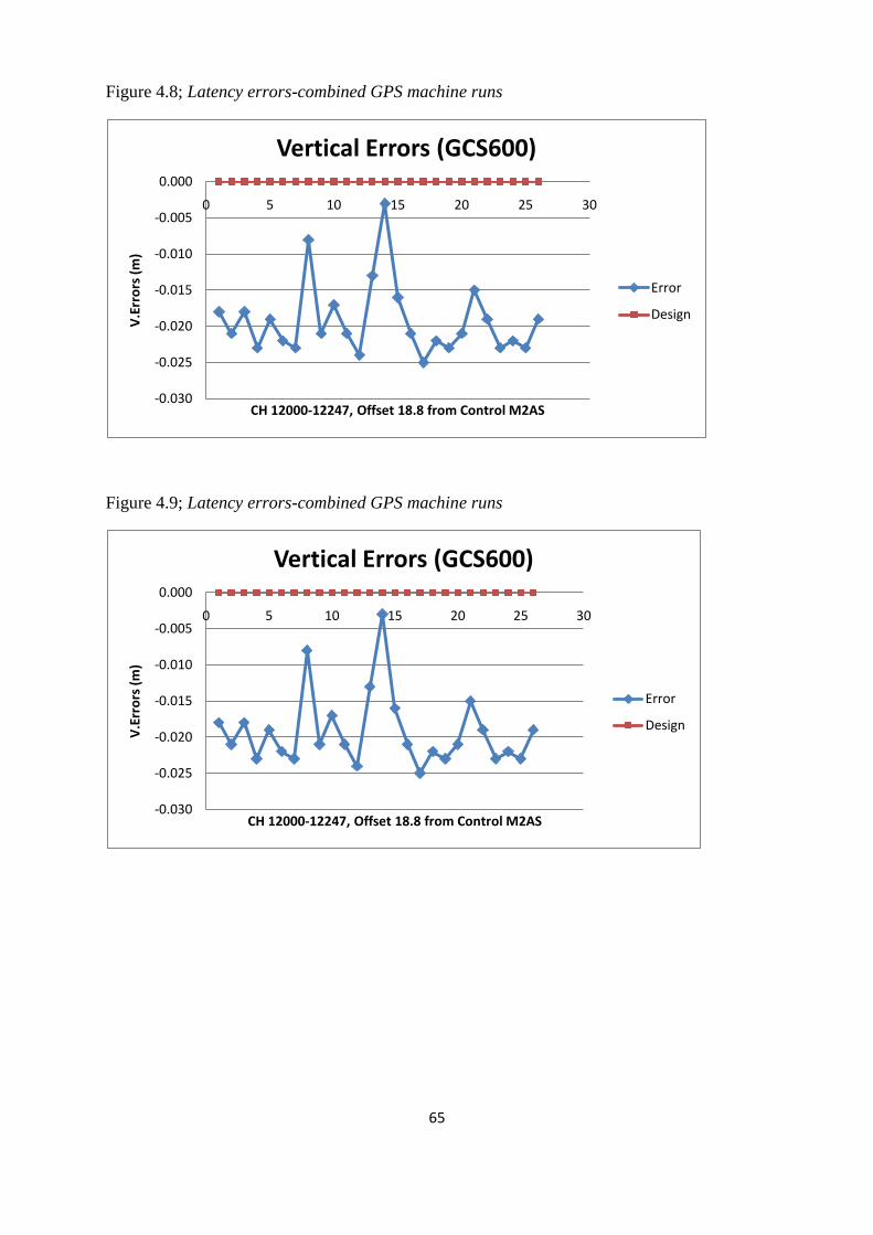
65



-0.030

-0.025

-0.020

-0.015

-0.010

-0.005

0.000

0 5 10 15 20 25 30

V.E

rro

rs (

m)



Error

Design

-0.030

-0.025

-0.020

-0.015

-0.010

-0.005

0.000

0 5 10 15 20 25 30

V.E

rro

rs (

m)



Error

Design

66



4.5.2 Trimble ATS5600 results

Figure 4.12 illustrates the errors associated with each point captured during testing. It

highlights that there is no systematic error present and the data was ranging between 0.000m

to 0.003 as figure 4.12 shows. Also figures 13 to 18 which are general capture, showing the

errors in the whole section.

-0.030

-0.025

-0.020

-0.015

-0.010

-0.005

0.000

0.005

0.010

0.015

0 5 10 15 20 25 30

V.E

rro

rs (

m)



Error

Design

-0.030

-0.025

-0.020

-0.015

-0.010

-0.005

0.000

0.005

0.010

0.015

0.020

0.025

0 5 10 15 20 25 30

V.E

rro

rs (

m)



Error

Design

67





moving target.

The graph also clearly illustrate that, as the tracking speed of the instrument is increased the

accuracy of points captured decreases because of the fact that the instrument is set far away

from the moving machine , although it does not appear to be significant at this stage.

Figure 4.12, vertical errors during 50m interval check.

Figure 4.13; Latency errors-combined ATS Total stations machine runs

-0.0005

0

0.0005

0.001

0.0015

0.002

0.0025

0.003

0.0035

1 2 3 4 5 6

V.e

rro

rs (

m)

50m interval comparison ATS Grader operator and Surveyors Leica Total station

Trimble 5600ATS Vertical error

Operator

Surveyor

-0.015

-0.01

-0.005

0

0.005

0.01

0.015

0.02

1 3 5 7 9 11 13 15 17 19 21 23 25 27

V. E

rro

r (m

)


Vertical Errors (ATS 5600)

Design

68



-0.02

-0.015

-0.01

-0.005

0

0.005

0.01

0.015

0.02

0.025

1 3 5 7 9 11 13 15 17 19 21 23 25 27

V.E

rro

r (m

)



Error

Design

-0.02

-0.015

-0.01

-0.005

0

0.005

0.01

0.015

0.02

0 5 10 15 20 25 30

V. E

rro

rs (

m)



Error

Design

Linear (Design)

69



-0.020

-0.015

-0.010

-0.005

0.000

0.005

0.010

0.015

0 5 10 15 20 25 30

V. E

rro

rs (

m)



Error

Design

-0.02

-0.015

-0.01

-0.005

0

0.005

0.01

0.015

0.02

0 5 10 15 20 25 30

V. E

rro

rs (

m)



Error

Design

70


4.6 Summary of results

A brief summary of GPS and ATS Total station tests are described on this section. Chapter 4

has presented the method of data analysis that has applied to the data captured as a result of

implementation of the methodology and examples outlined on chapter 3. This is the complete

description of the methods required to extract useful information regarding latency, position

vertical errors in dynamic RTK and ATS total station measurements from raw data files

attained in the implementation of the research methodology.

This chapter has also demonstrated that latency is affecting the results that have been

obtained from the testing carried out as an integral component of this research. As such, it

becomes more important that a further investigation of this effect is thoroughly undertaken;

over a greater range of speeds allow potential users to achieve their goals in real time.

As the first chapters elaborated the aim of this project is to determine the accuracy and

reliability of machine guidance. Since this project is dealing with one type of instruments; i.e.

Trimble ATS5600 Total station and GCS600 GPS systems, it‟s hard to draw a final

conclusion of the errors and reliability during and after field operations.

However, based on the above tests it can be concluded that, the reliability of ATS is greatly

related to the speeds of the prism and measurements distances. The ATS tends to lose lock in

the higher speed environment at short distance. Also the ATS may not reflect the true centre

of the target and this may result in false or bad answer.

Chapter 5 summarises the current status of this research and makes recommendations

regarding the continuation of this research project, and also the adaption of methodology

described on chapter 3 to different level of speed application.

-0.015

-0.01

-0.005

0

0.005

0.01

0.015

0.02

0 5 10 15 20 25 30V.E

rro

rs (

m)



Error

Design

71

4.7 Discussion

4.7.1 Reliability

The reliability of ATS is closely associated with the movement speeds and the distance

between setup station and observations area (grader). It has been described earlier that, ATS

tends to lose locks in higher speed environment or shorter distance or any other factor.

The accuracy of the results it depends upon the speed of the prism and the experience of the

grader operator. The accuracy of the observed data will reduce and sometimes may lead to

the dropout signal. The ATS may resume lock to the target within a very short period of time

but the result obtained as the asbuilt survey will be affected as there is a lapse in observation

result caused by loose lock.

Chapter 4 has also outlined the data analysis process required to extract useful information

from the data that collected upon implementation of testing regime developed on this

research project, to quantify the latency error in speed environment when using a moving

GPS. Chapter 4 also demonstrated that there is some latency error in the gathered data.

4.7.2 Accuracy of Tracking

The accuracy of the ATS it‟s widely depends on prism pointing. If the ATS is not pointing

towards the centre of the prism, as described by Stempfhubber at al. (2001), it may lead to

large variations in the observation results. As pointed out by Kopacic, (1998), the ATS

should always be measuring to the centre of the prism, see also figure 2.13 and notes 2.5.7

Auto search.

If the prism is moving along the path and the ATS is not pointing directly to the prism, then

the measured value will have a large variations impact when analysis of results takes place.

Standard total stations are optimized for static prism measurement; in contrast,

synchronization of data from the angle and distance measurement sensors allows output data

to be computed for a single instantaneous location of the moving machine. This results in

higher 3D position accuracy for dynamic measurements or machine tracking application.





moving target.

Low latency for complete transmission the precise position of the machine at any given time

depends on the age or latency of the positioning data received, if the age of the data is recent

and specific.

72

CHAPTER 5

CONCLUSION AND RECOMENDATIONS

5.1 Introduction

Several issues have been arisen during this research project and needs to be addressed in the

future to come. Chapter five provides an outline of the current status of the research, and also

makes the recommendations regarding the continued research and investigation of latency

errors in RTK and ATS.

5.2 Further Research and Recommendations

5.2.1 Testing GCS600 GPS

Following the methodology described in chapter 3, this dissertation has only been possible to

utilise GC600 conventional RTK GPS due to the time constraints. Further research efforts

required in this specific field of Machine guidance latency measurements, to implement this

testing in similar fashion, to analyse the resulting data (in accordance with the practice

described herein) to give potential Machine guidance users and understand the effect of

latency in high and low speed environment. These effects should then be compared to the

results obtained in this research.

5.2.2 Additional device (Laser augmented RTK GPS)

As previously mentioned, this research project has also led to the discovery that it is possible

to utilise the addition devices that are solid based on their ability to increase the vertical

precision of RTK GPS. Such devices are; Laser Augmented Systems (on blade), see also

chapter 2.2.5.

It is therefore that part of future recommendations on this research project is to have a future

version of Laser Augmented RTK GPS which is attached in an onboard software package

than having an external devices which increases the weight of the blade if can (this

information has been passed on to the manufacturer) .

In advanced cases, the onboard computer can be directly linked to the machine hydraulics,

controlling their operation with minimal input from operator.

In addition, value sensors can be added for fully automatic machine control. The slope and

elevation of the blade are therefore controlled by the system, not by the machine operator

reducing errors and avoiding expensive re-work. These methods are still new in the market

and needs more future research because the accuracies and tolerances are still not yet known.

73

5.2.3 Testing at Speeds

According to previous testes described in the previous chapters that, testing is required up to

250km per hour in order to be of use to the precision agricultural community. Therefore

future testing is required to investigate latency‟s and its effect on speeds application to gain

more understanding of the relationship. The use of an optional sensor is seen as a very

accurate means of referencing the dynamic measurements back to the fixed frame of

reference and has therefore been adopted for this research project also.

The methodology and techniques may be used for future testing based on what is described in

this dissertation. But it is recognised that modification of this equipment configuration and

testing regime is required to facilitate this.

5.2.4 Testing Trimble ATS5600

As mentioned earlier in the previous chapters that, due to the time constraints there was only

one type of ATS Total station being tested throughout duration of this project and backed up

by Leica Total station for data recording. The results shown on chapter 4 were based on

Trimble ATS total station.

Similar testes have been conducted before and more research investigations are

recommended should be undertaken in order to obtain more accurate results.

It has been recommended by Trimble (2004), that the minimum distance to the survey

instrument should be atleast 100m for a moving speed of less than 5m/sec. During testing ,

the moving speed was almost the same as stated speed however the ATS seemed to achieve a

great results regardless to the changes of weather.

5.3 Conclusion

These days, the major applications of 3D machines guidance can be found in the construction

and mining industries for the guidance of dozers, rollers, graders, excavators and tractors. As

mentioned earlier, the ATS, RTS have been in the market since 1990s and yet still a little

information‟s available about their real time operations.

It has been pointed out by Retscher, (2002) that for the guidance of road and paving machine,

high precision requirement for the height components are still very challenging for the 3D

machine guidance systems. In order to achieve this level of precision and replace

conventional labour intensive in this type of application, present 3D systems require further

improvement.

There is a limitation of ATS when carrying out measurements. The ATS does not point direct

to the centre of the prism. This could be one of the causes of the errors during field

operations.

74

Approximately 94% of the measured value tests have passed the manufactures specification

for ATS total stations and 91% for the Trimble GPS. The accuracies achieved by ATS5600

Total station and GPS would comply with the majority of construction accuracy

requirements. The reliability of the instruments is also good under these conditions with only

10 percent falling outside the manufactured specifications.

Chapter 5 presents various recommendations regarding possible future direction for ongoing

research into the effect of latency when using machine guidance. The methodology

developed in this dissertation required for future continuation of further research to

investigate the effect of latencies when using machines guidance.

In conclusion, the author believes that the latency caused by distance time measurements in

ATS is the most critical factor associated with an ATS performance in terms of accuracy and

reliability.

BIBLIOGRAPHY

Campbell, J, Carney, C., Kantowiz, B., 1998, Human Factors Design Guidelines For

Advanced Traveler Information Systems (Atis) And Commercial Vehicle Operations (Cvo),

Vehicle Location Accuracy, Battelle Human Factors Transportation Centre 4000 NE 41st

Street Seattle, WA. [online], Available from:

http://www.fhwa.dot.gov/tfhrc/safety/pubs/atis/ch05/ch05_10.html

[Viewed May 01, 2010]

Gibbings P., O‟Dempsey A., 2005, using GPS Asset Mapping Software for Hydrographic

Measurements in Still Water, Journal of the Spatial Sciences Institute (QLD).

Trimble Navigation, 2010, Trimble Virtual Reference Station (VRS) System (data sheet),

Available from:

http://trimble.com/docushare/dsweb/Get/Document-11465/VRS_spec_sheet.pdf

www.trimble.com(ATS_DS_022482112B_09021.pdf

-Trimble 5600 Series User Guide (SECURED)


Geodimeter (2003), Robotic Total Station and Sensor for Machine Control “ One Instrument-

Countless Applications”, Technical Notes, Danderyd, SWEDEN.

Available:

http://www.spectraprecision.com


http://www.fhwa.dot.gov/tfhrc/safety/pubs/atis/ch05/ch05_10.html

http://trimble.com/docushare/dsweb/Get/Document-11465/VRS_spec_sheet.pdf

http://www.trimble.com(ats_ds_022482112b_09021.pdf/

http://www.spectraprecision.com/

75

Gomac (2002): Stringless Guidance System. Technical Notes, Gomaco corporation, Ida

Grove, Iowa, USA.

Available: http://www.gomaco.com/Resources/Leica.html


Gunter Retscher (1995), Three dimensional Surveying of a Railway track using a multi

sensor system and optional linear estimation methods. Vienna University of Technology.

Gunter Retscher (2000), Trajectory Determination for Machine Guidance Systems. Papers

presented at the KIS2001 Symposium, 5-9th

June 2001, Banff, Canada.

Available: http://info.tuwien.ac.at/ingeo/pub/papers/kis.pdf


Iveta Ceryova, Patrick Kubanka, Dr. Alojz Kopaeik and Peter Kyrinovie (2002), Dynamic

Tests of Robotic Stations .Paper presented at International Congress, 19-26 April 2002,

Washington, D.C. USA.

Manufacturer RTK Equipment Specifications and GPS notes.

Department of spatial science, Curtin University.

http://spatial.curtin.edu.au/research/

[Viewed April 10, 2010]

University of Southern Queensland, 2006, Automated Surveying Systems, University of

Southern Queensland, Australia

APPENDICES

APPENDIX A; Project Specification

http://www.gomaco.com/Resources/Leica.html

http://info.tuwien.ac.at/ingeo/pub/papers/kis.pdf

http://spatial.curtin.edu.au/research/

76


FACULTY OF ENGINEERING AND SURVEYING

ENG 4111/4112 Research Project

PROJECT SPECIFICATION

FOR: Said Kiongoli

TOPIC: TESTING THE ACCURACY OF MACHINE GUIDANCE IN ROAD

CONSTRUCTION.

SUPERVISOR: Mr Shane Simmons

SPONSORSHIP: Multi Surveying Company

PROJECT AIM: The aim of this project is to test the accuracy and reliability of Machine

Guidance when used in road construction.

PROGRAMME: (Issue A, 23rd

March 2010)


2. Review existing history concerned Real time and manual guidance systems.

3. Establish and conduct a series of testing under various conditions.

3. Undertaking analysis of test results and determining the final accuracies of machine

guidance systems.

6. Conclusion and submit an academic dissertation on the research.

As time permits:

7. Research a better system (Machine Guidance) that will reduce the errors in road

construction industry.

AGREED:

Said Kiongoli (Student) ________________, ________________ (Supervisors)

23/03/2010 ___/___/______ ___/___/______

Examiner/Co-examiner: _______________________________________

77

APPENDIX B; Safe Work Method Statement and Risk Assessment

80

APPENDIX C; Cross Sections

87

APPENDIX C; Trimble ATS5600 Notes

89

APPENDIX D: Trimble GC600 Notes

91

APPENDIX E: Digital Terrain Modal (DTM or TIN)

Tin or DTM created using 12d software

testing the accuracy of machine guidance in road construction

Documents