testing nutrient ﬂushing hypotheses at the hillslope scale

Testing nutrient flushing hypotheses at the hillslope scale:

A virtual experiment approach

Markus Weiler*, Jeffrey J. McDonnell

Departments of Forest Resources Management and Geography, University of British Columbia,

2037-2424 Main Mall, Vancouver, BC, Canada V6T 1Z4

Received 4 August 2004; revised 30 June 2005; accepted 30 June 2005

Abstract

The delivery mechanisms of labile nutrients (e.g. NO3, DON and DOC) to streams are poorly understood. Recent work has

quantified the relationship between storm DOC dynamics and the connectedness of catchment units and between pre-storm

wetness and transient groundwater NO3 flushing potential. While several studies have shown N and C flushing during storm

events as the important mechanism in the export of DOC and DON in small catchments, the actual mechanisms at the hillslope

scale have remained equivocal. The difficulty in isolating cause and effect in field studies is made difficult due to the spatial

variability of soil properties, the limited ability to detect flow pathways within the soil, and other unknowns. Some hillslopes

show preferential flow behavior that may allow transmission of hillslope runoff and labile nutrients with little matrix

interaction; others do not. Thus, field studies are only partially useful in equating C and N sources with water flow and transport.

This paper presents a new approach to the study of hydrological controls on labile nutrient flushing at the hillslope scale. We

present virtual experiments that focus on quantifying the first-order controls on flow pathways and nutrient transport in

hillslopes. We define virtual experiments as numerical experiments with a model driven by collective field intelligence. We

present a new distributed model that describes the lateral saturated and vertical unsaturated water flow from hypothetical finite

nutrient sources in the upper soil horizons. We describe how depth distributions of transmissivity and drainable porosity, soil

depth variability, as well as mass exchange between the saturated and unsaturated zone influence the mobilization, flushing and

release of labile nutrients at the hillslope scale. We argue that this virtual experiment approach may provide a well-founded

basis for defining the first-order controls and linkages between hydrology and biogeochemistry at the hillslope scale and

perhaps form a basis for predicting flushing and transport of labile nutrients from upland to riparian zones.

q 2005 Elsevier Ltd All rights reserved.

Keywords: Virtual experiments; Hillslope hydrology; Nutrients; Mobilization; Flushing; Runoff generation

0022-1694/$ - see front matter q 2005 Elsevier Ltd All rights reserved.

doi:10.1016/j.jhydrol.2005.06.040

* Corresponding author. Tel.: C1 604 822 3169; fax: C1 604 822

9106.

E-mail address: [email protected] (M. Weiler).

1. Introduction

The hydrological controls on the flushing of labile

nutrients at the hillslope and headwater catchment

scale are still poorly understood. Several studies have

shown that stream DOC concentrations often peak on

Journal of Hydrology 319 (2006) 339–356

www.elsevier.com/locate/jhydrol

http://www.elsevier.com/locate/jhydrol

M. Weiler, J.J. McDonnell / Journal of Hydrology 319 (2006) 339–356340

the rising limb of the snowmelt and rainfall-induced

hydrographs, prior to peak discharge, followed by a

rapid decrease in concentrations following rainfall

cessation or melt decline (Boyer et al., 1997;

Hornberger et al., 1994). Creed and Band (1998a,b)

and Inamdar et al. (2004) found a similar trajectory in

nitrate concentrations for both spring snowmelt and

autumn rainfall events.

These and other studies have attributed the early

peaks in the nutrient concentrations to the Hornberger

et al. (1994) ‘flushing’ hypothesis, which is also based

on earlier studies, for example, by Pinder and Jones

(1969); Anderson and Burt (1982), whereby nutrients

are leached from near-surface layers by a rising water

table (Weyman, 1973) followed by a quick lateral

transport of these leached nutrients to the stream via

near-surface subsurface stormflow on the hillslope or

surface, saturation excess runoff in the riparian zone.

This rapid delivery of nutrients with surface runoff is

often assumed to explain the early expression of these

nutrients on the discharge hydrograph. Hydrologi-

cally, a key feature of this perceptual model is full-

column saturation of the soil profile or at least water

table rise high enough into the soil profile to encounter

near-surface soils with high transmissivity and hence,

potential for significant lateral flow to occur. This so-

called transmissivity feedback is now a common

hypothesis to explain lateral flushing of labile

nutrients (Bishop et al., 2004). A key requirement of

the ‘flushing’ hypothesis biogeochemically, is the

ready availability of excess nutrients in the near

surface soil horizons—now axiomatic of soil biogeo-

chemical environments (Lajtha et al., 2004; Qualls

and Haines, 1991) and labile nutrient concentration

profiles in undisturbed environments.

Notwithstanding these gross generalities, obser-

vations of event-scale hydro-biogeochemical flushing

and draining are highly complex, often contradictory

from catchment to catchment and highly equivocal

overall. Recent work has revealed distinct hillslope

versus riparian control on DOC flushing (McGlynn

and McDonnell, 2003) whereby a rainfall or ante-

cedent wetness threshold is necessary to activate

measurable hillslope contributions to streamwater

DOC concentrations. Some studies have observed

distinct hotspots in and around the hillslope–riparian

zone interface for exfiltration of elevated DOC

concentrations (Hinton et al., 1998). For nitrate,

Burns et al. (1998) observed that deep groundwater

flow from distinct springs controlled summer nitrate

concentrations in the channel. Similarly, Hill et al.

(1999); McHale et al. (2002) did not find any evidence

of nitrate flushing. Hill et al. (1999) identified

throughfall as the principal contributor to stream

nitrate. McHale et al. (2002) found that groundwater

springs, which discharged deep till groundwater,

controlled the stream nitrate chemistry during events.

Moreover, McHale et al. (2002) also observed nitrate

peaks on the rising limb of the stream discharge

hydrographs for some summer/autumn storm events,

but in contrast to Creed and Band (1998b), attributed

the early nitrate expression to the quick displacement

of till water by infiltrating rainwater.

In terms of studies more in line with the classical

flushing hypothesis, the literature is still quite uneven

on cause and effect. Welsch et al. (2001) observed

staggered nitrate and DOC peaks during a summer

storm event—with a nitrate peak on the rising limb

and a delayed DOC peak, which followed the

discharge peak (Fig. 4 in Welsch et al., 2001).

Following the Creed and Band (1998a,b) rationale,

Welsch et al. (2001) speculated that nitrate was

flushed from the hillslope but they did not present any

direct evidence to support this conclusion. Brown

et al. (1999) working in the same Catskill New York

catchments as Welsch et al. (2001); Burns et al.

(1998) reported summer DOC peaks which occurred

after the peak in discharge and DOC concentrations

which were greater on the recession limb than those

on the hydrograph rising limb. Brown et al. (1999)

were not able to explain the lag in DOC concen-

trations but attributed the high DOC concentrations to

hillslope O-horizon soil waters. In a forested

catchment in Germany, Hangen et al. (2001) also

found delayed DOC contributions that occurred after

peak discharge. Hangen et al. (2001) hypothesized

that the delay in DOC expression was due to the time

lag associated with the onset of streamflow, which

displaced DOC rich waters from the hillslope to the

stream via macropores.

So what can be generalized from these studies?

Perhaps, it is the one-dimensional behavior that is

most clear. While the biogeochemistry of DOC, DON

and NO3 is complex and different for each nutrient

form, concentrations are often found to decrease

markedly with depth through the soil profile

M. Weiler, J.J. McDonnell / Journal of Hydrology 319 (2006) 339–356 341

(Bishop et al., 2004; Worrall and Burt, 1999). Results

of the DIRT experiments (Lajtha et al., 2004) suggest

that this decrease is often exponential. At the plot

scale, soil hydraulic conductivity also declines with

depth and soil bulk density increases with depth. This

commonality may drive the response at the plot scale.

Identification of the first-order controls on the flushing

behavior remains highly equivocal in the published

literature. This is further exacerbated by added

complexity in how processes scale from the plot to

the hillslope, from the hillslope to the riparian zone

and at other key ecotonal boundaries elsewhere in the

catchment. Sometimes elevated DOC concentrations

appear to be displaced from the riparian zone (Hinton

et al., 1998). Sometimes preferential flow is argued as

the control on NO3 flushing laterally at the hillslope

scale (Buttle et al., 2001).

In this paper, we argue that for progress to be made

in understanding the hydrological controls on labile

nutrient flushing, we need to worry less about the

complexities of individual hillslopes and need to

concentrate on first-order effects. We use the concept

of virtual experiments (Weiler and McDonnell, 2004)

in this paper as a way to filter out non-essential

elements. We acknowledge that our model is an

extreme simplification of both the hydrological

processes and biogeochemical processes operating.

Therefore, the virtual experiment is not an attempt to

‘model the system’ but is rather a tool to understand a

phenomenon. We use the model as a learning tool and

adhere to Occam’s Razor, whereby the simplest

explanation that can account for the phenomenon is

the best explanation. In this way, the virtual

experiment is therefore another research tool that

can be applied to the problem, in addition to more

traditional field experimental and computer

modelling.

Our overall objective of this paper is to answer the

question “what is the effect of hillslope shape and

antecedent wetness on nutrient mobilization”. Specifi-

cally, we test for planar hillslopes and for concave

hillslopes (where a riparian zone exists at the slope

base) and explore (1) the importance of the

transmissivity feedback hypotheses in flushing nutri-

ent in shallow soils compared to other hypotheses

(e.g. preferential flow), (2) the connection between

hillslope and riparian zone, and (3) the use of

concentration–discharge relationship to understand

nutrient mobilization processes.

2. Theory and methods

2.1. Hill-vi

We use the physically-based hillslope model Hill-

Vi as the framework for performing the virtual

experiments to explore the first-order controls on

nutrient flushing at the hillslope scale. The basic

concepts of Hill-Vi are described in detail in Weiler

and McDonnell (2004). Here, we review only briefly

the basic model structure and then introduce in some

detail the transport modeling component that is new to

this paper. The model is based on the concept that a

saturated and unsaturated zone defines each grid cell,

based on DEM and soil depth information. The

unsaturated zone is defined by the depth from the soil

surface to the water table and time variable water

content. The saturated zone is defined by the depth of

the water table to an impermeable soil–bedrock

interface and the porosity n. Lateral subsurface flow

is calculated using the Dupuit-Forchheimer assump-

tion and is allowed to occur only within the saturated

zone. Routing is based on the grid cell by grid cell

approach (Wigmosta and Lettenmaier, 1999) using

the water table slope as the driving force. The depth

dependence of the hydraulic conductivity in the soil

profile can either be described by an exponential

function or by a power law function (Weiler and

McDonnell, 2004).

We selected the exponential function for soil

hydraulic conductivity depth dependence for these

virtual experiments. While these assumptions and

model implementations are similar to existing models

like DHSVM (Wigmosta et al., 1994) and RHESSys

(Tague and Band, 2001), we also introduced a depth

function for drainable porosity—a parameter shown

to be a key first-order process control on transient

water table development (Weiler and McDonnell,

2004). The drainable porosity is defined by the

difference in volumetric water content between the

saturated water content and the water content at a soil

water tension of 100 cm (approximately field

capacity). Field observations show that the drainable

porosity usually declines with depth due to changes in


the soil structure and macropore development and

presence (see, for example, data in Ranken, 1974;

Rothacher et al., 1967; Weiler, 2001; Yee and Harr,

1977). Thus, a depth function for drainable porosity nd

can be defined as

ndðzÞ Z n0 exp Kz

b

� �(1)

where n0 is the drainable porosity at the soil surface, z

is the soil depth measured from the soil surface and b

is a decay coefficient.

We calculate the water balance of the unsaturated

zone by the precipitation input, the vertical recharge

loss into the saturated zone, and the change in water

content. Recharge from the unsaturated zone to the

saturated zone is controlled by a power law relation of

relative saturation within the unsaturated zone and the

saturated hydraulic conductivity at water table depth

w (measured form the soil surface) and a power law

exponent (Weiler and McDonnell, 2005). The water

balance of the saturated zone is defined by the

recharge input from the unsaturated zone, the lateral

inflow and outflow by lateral subsurface flow and the

corresponding change of water table depth. Evapor-

ation losses from the surface are neglected in this

application. Since drainable porosity is not constant

with depth, the water balance of the saturated zone

was solved for the exponential model of the drainable

porosity (Weiler and McDonnell, 2005).

Hill-Vi includes a relatively simple solute

transport routine as described by Weiler and

McDonnell (2005). We extend this feature in this

paper for exploring the controls on nutrient

flushing. We assume complete mixing within each

grid cell separated for the saturated and unsaturated

zone and only advective transport in and between

the saturated and unsaturated zone and in and

between grid cells. Field data of labile organic

nutrient concentrations in undisturbed soils (e.g.

forest soils) show a distinct decline with depth

(e.g. DOC and DON in Swiss forest soils

(Hagedorn et al., 2001), TOC in Swedish forest

soils (Bishop et al., 2004)). We used this quite

common experimental evidence to define a depth

distribution of nutrient concentration c in soil water

cðzÞ Z c0 exp Kz

bm

� �(2)

where c0 is the nutrient concentration at the soil

surface and bm is the decay coefficient. This

concentration profile defines the initial conditions

and c0 is changing, but bm remains constant

according to the solute mass in the unsaturated

zone (Eq. (8)). We can calculate directly the solute

mass in the unsaturated zone assuming a uniform

moisture content profile depending on the concen-

tration distribution and the water table w, defining

the vertical extent of the unsaturated zone:

Mun Z qc0bm 1Kexp Kw

bm

� �� (3)

When simulating water and solute flux within

Hill-Vi, we assume that the shape of the concen-

tration profile remains essentially constant (bmZconstant). The actual mass in the unsaturated and

saturated zone however, changes depending on the

mass flux, as calculated below. A large preponder-

ance of experimental evidence shows that the

concentration of water draining out of a zero

tension lysimeter is similar to the average concen-

tration in the unsaturated soil (Jemison and Fox,

1994; Murdoch and Stoddard, 1992). Thus, solute

flux in recharge mr depends on the average

concentration in the unsaturated zone and can be

determined by

mrðtÞ Z RðtÞMunðtÞ

SunðtÞ(4)

where R(t) is the recharge in one grid cell at time t

and Sun is the water storage in the unsaturated zone

that is the product of the water table depth and the

water content in the unsaturated zone. The solute

flux in the lateral subsurface flow from one grid

cell to the next is calculated in a similar fashion by

multiplying the subsurface flow with the actual

concentration in the saturated zone.

Weiler and McDonnell (2004) introduced a new

concept to simulate the mass exchange between the

saturated and unsaturated zone under a changing

water table. In this paper, we further developed this

concept by including the depth distribution of

drainable porosity (Eq. (1)) and the depth distribution

of nutrient concentration into the mass exchange

calculation. Weiler and McDonnell (2004) showed

that under a falling water table, solutes are transferred

(Dm) from the saturated to the unsaturated zone


depending on the concentration in the saturated zone,

the water table change (Dw) and the difference

between total porosity and drainable porosity (that is

the proportion of water that is drained by the falling

water table). Since the drainable porosity is variable

with depth (it was assumed to be constant in Weiler

and McDonnell, 2004), we must first calculate the

average drainable porosity �nd between the water table

at time t and the water table in the previous time

step by:

�nd Zn0b

DwðtÞexp K

wðtÞCDwðtÞ

b

� �Kexp K

wðtÞ

b

� ��

(5)

The solute transfer under a falling water table from

the saturated to the unsaturated zone can then be

calculated by

DmðtÞ ZMsatðtÞ

ðDKwðtÞÞneff

DwðtÞðnK �ndÞ (6)

where D is the soil depth and the actual mass of

solutes in the saturated zone is defined by Msat, and the

effective porosity by neff. The effective porosity is a

common simplification describing the porosity avail-

able for fluid flow (Bear, 1972).

If the water table is rising, Weiler and McDonnell

(2004) showed that the mass transfer depends on the

concentration in the unsaturated zone. They assumed

an average concentration in the unsaturated zone to

calculate the mass exchange. However, for using the

model in application to labile nutrients, we introduce a

depth distribution function for nutrient concentration.

To account for this distribution, we must acknowledge

a clear and transparent (and simple) way to

conceptualize the probable hydrobiogeochemical

processes under a rising water table condition. We

assume that the rising water table can only mobilize

the nutrients within the depth of the water table. Thus

the actual nutrient concentration at the water table

defined by the exponential depth distribution deter-

mines the solute exchange

DmðtÞ ZMunðtÞ

SunðtÞexp K

wðtÞ

bm

� �DwðtÞðnK �ndÞ (7)

We can now calculate the solute mass balances

for the unsaturated and saturated zone within each

grid by

MunðtÞ Z MunðtKDtÞKDmðtÞKmrðtÞ (8)

MsatðtÞ Z MsatðtKDtÞCDmðtÞCmrðtÞCmssfðtÞ

(9)

where mssf is the mass flux due to the lateral

subsurface flow.

2.2. Virtual experiment design

Designing a virtual experiment requires much pre-

experimental dialog and interaction between the

experimentalist and the modeler. The exercise is not

one of fitting parameters to an existing experimental

output, but a procedure to explore first-order effects of

model decisions on ‘measured’ response. This often

follows on from intensive field campaigns where

the experimentalist may have a highly complex yet

quantitative view of hillslope runoff generation. The

virtual experiments reported in this paper are based on

the design presented below. While these experimental

design criteria will no doubt change from experiment

to experiment, we present these details as an example

that one might conduct and in doing so, exemplify our

approach for this chosen case.

2.2.1. Hillslope topography and antecedent wetness

conditions

As per our stated objectives in this paper, we test

the effects of hillslope shape and antecedent wetness

conditions on nutrient flushing by defining two

different hillslope shapes and two different antecedent

wetness conditions. Since the main objective vis-a-vis

hillslope shape was to explore the effect of a hillslope

with and without a riparian zone, we simply define a

hillslope by a straight slope profile and a hillslope

with a riparian zone at the slope base by a concave

slope profile, calculated by

zðxÞ Z xatan bxmax

xamax

(10)

where x is the length in direction of the slope, z the

surface elevation, xmax is the maximum hillslope

length, tan b is the slope, and a is the exponent

defining the profile curvature. For the concave

curvature aZ2.0; for the straight profile aZ1.0. The

slope for both hillslopes was set to 30% and the total


length to 100 m. These values are quite typical for

hillslopes in forested headwaters in the USA Pacific

Northwest (e.g. the HJ Andrews Experimental Forest)

and other Pacific Rim sites where we have worked

(e.g. the Maimai watershed, South Island New

Zealand).

In order to account for the different antecedent

wetness conditions, we saturated the two different

hillslopes and simulated drainage without any further

rainfall input for 5 days for the ‘wet antecedent

condition’ and for 20 days for the ‘dry antecedent

conditions’. This procedure created initial conditions

shown in Table 1 for the four different experiments:

straight slope-dry antecedent conditions, straight

slope-wet antecedent conditions, concave slope-dry

antecedent conditions, and concave slope-wet ante-

cedent conditions.

2.2.2. Soil properties

One common problem of transferring the exper-

imental results from one site to another is that either

the soil properties change or the slope geometry is

different. The advantage of the virtual experiment is

that, for example, the hillslope geometry can remain

constant but the soil properties can change and vice

versa. The virtual experiment design in this paper

explores only the effect of hillslope shapes and

antecedent wetness conditions. Thus the soil proper-

ties were held constant from experiment to exper-

iment. The physical soil properties used here are

based on measured data from the H.J. Andrews

Experimental Forest, USA (Ranken, 1974). The

resulting values are for the drainable porosity at the

soil surface n0Z0.09 with a shape parameter bZ1.5.

The saturated hydraulic conductivities at the soil

surface are KsatZ1.7!10K4 m sK1, the total and

effective porosity are 30%, and the transmissivity

Table 1

Initial conditions for the four virtual hillslope experiments

Hillslope

shape

Antecedent

conditions

Average water storage (mm)

Unsaturated

zone

Saturated

zone

Straight Dry 192 105

Wet 189 180

Concave Dry 185 125

Wet 175 205

profile was defined by an exponent of 3.0. For

simplicity, we assumed the soil depth constant within

the hillslope with a depth DZ2.0 m. The boundary

condition at the upper end of the slope was set to ‘no

flow’ and the boundary at the lower end of the slope

was set to a fixed water level, imitating a constant

water level in a stream.

The shape parameter (bmZ0.5) for the concen-

tration depth distribution for a nutrient like DOC was

derived from data of DOC in forest soils (as reported

by Hagedorn et al., 2001 and many others). In order to

avoid any specification of nutrient concentrations in

the soil, we set an arbitrary initial average concen-

tration of 1.0 g/l, resulting in a c0Z4.0 g/l for the 2 m

deep soil profile. The initial mass in the unsaturated

and saturated zone was then calculated assuming

equilibrium conditions (see also Eq. (3)). In this

simplified experiment, we treat the nutrients as a

conservative solute, thus ignoring production, sorp-

tion etc. We can support this rationale by focusing

strictly at the event time scale. If we were to look over

longer time scales, these issues would likely become

important to the coupled hydrobiogeochemcial

behavior.

2.2.3. Precipitation time series

To understand nutrient flushing, draining and

mobilization under natural conditions, we selected a

rainfall time series from a climate station in the Pacific

Northwest (Eugene WSO Airport, Oregon 352709).

We selected a 500 h time window (starting Oct 1st,

1984) with a total rainfall of 236 mm and five

distinctive rainfall events. This time series is typical

for the rainy season during fall/winter in Oregon,

when frontal storms with relative low rainfall

intensity are moving in from the Pacific Ocean.

3. Results

The results from the virtual experiments are

divided into three sections. In the first section, we

present the results from the four experiments by

linking the simulated flow and concentration response

at the base of the hillslope with the internal spatial–

temporal response within the hillslope. These data

are used to provide a general understanding of

event processes. In Section 3.2, we will present


the concentration–discharge data for the same

experiments. These C–Q plots are a well-established

way in the experimental literature to analyze nutrient

behavior in watersheds in relation to streamflow

response (Anderson et al., 1997; Buttle et al., 2001;

Evans and Davies, 1998; Hall, 1970; Lawrence and

Driscoll, 1990). The last section explores more

specifically the time and geographic sources of the

slope base nutrient export, testing different flushing

hypotheses on nutrient flux from the planar hillslope

and its relation and connectedness to the hillslope–

riparian zone interface.

3.1. Flow and concentration response

The simulated flow and concentration response at

the base of the hillslope together with the spatial–

temporal response within the hillslope for the

experiment with a straight hillslope under dry

antecedent soil moisture conditions (straight-dry) is

shown in Fig. 1. The upper panel shows the rainfall

time series together with the simulated average

recharge within the slope and the lateral subsurface

flow at the base of the hillslope. Recharge responds

rapidly to storm rainfall, especially for the last event

under the wetter soil conditions. The resulting

subsurface flow is delayed relative to recharge but

still shows a storm related response. This is in keeping

with how we might conceptualize the sequence of

conversion of vertical to lateral flow on a hillslope

(Tromp-van Meerveld, 2004). The next panel shows

the average concentration in recharge, subsurface

flow and in the saturated and unsaturated zone. It is

important to note that concentrations in the unsatu-

rated and saturated zone change due to cell to cell

import and export of nutrients and also due to volume

change of the zones themselves (i.e. water table rise

and fall in the saturated zone and changing water

content in the unsaturated zone). The concentration

response in the unsaturated zone is significant, and

follows the general pattern of recharge; however, the

concentration response in the subsurface flow is low

by comparison and strongly lagged and damped.

While average concentrations in the unsaturated zone

generally decrease with time, saturated zone concen-

trations remain constant. The lower two panels show

the spatial-temporal response internal to the hillslope:

the horizontal axis shows time and the vertical axis

space (i.e. horizontal distance from the base of the

hillslope). The space axis is represented schematically

by the depicted cross-section of the hillslope on the

right side of the plot (light gray area is the soil, dark

grey area is the impermeable bedrock). These ‘slope

diagrams’ are rotated 908 to the right for ease of

seeing schematically how horizontal distance equates

to distance upslope.

The gray shaded regions in the time-space plots

(Fig. 1) show regions between two concentrations in

the vertical recharge flux (third panel) and the lateral

subsurface flux (fourth panel). The dashed and dotted

contours show lines of equal relative water content

(1.0Zsaturation) in the unsaturated zone (third panel)

and lines of equal relative water table height (0.0Zat

the soil–bedrock interface, 1.0Zat the soil surface).

The third panel for the unsaturated zone shows

relative spatially uniform water content changes, but

higher concentration in the recharge in the lower part

of the hillslope. In the fourth panel for the saturated

zone, water table response is more related to the

hillslope position and more delayed as the water

content response in the unsaturated zone. The

concentrations in the subsurface flow look quite

similar to the concentration in the recharge. In

general, the lateral subsurface stormflow and its

corresponding concentration response to rain are

weak and delayed.

The results for the second virtual experiment for

the straight hillslope under wet antecedent soil

moisture conditions (straight-wet) are shown in

Fig. 2, as per the same types of diagrams for

experiment 1. Not surprisingly, the recharge and

subsurface flow response are much more pronounced,

compared to the straight-dry experiment. The first

storms under the wetter initial conditions result in a

larger response. The concentration time series is also

more variable compared to the straight-dry exper-

iment, in particular for the recharge concentration.

Concentration in the subsurface flow is still constant.

Water content response in the unsaturated zone (third

panel) is strongly dependent on the rainfall intensity.

Also concentration in recharge is more dependent on

time. Nevertheless, there are some concentration

patterns for the first storms where the concentration

in recharge is much higher, especially closer to

the base of the hillslope. The water table response

(fourth panel) is faster and larger compared to the

Fig. 1. Results of the virtual experiment for the straight hillslope under dry antecedent soil moisture conditions (straight-dry). The upper panel

shows the rainfall time series together with the simulated average recharge within the slope and the lateral subsurface flow at the base of the

hillslope. The second panel shows the average concentration in recharge, subsurface flow and in the saturated and unsaturated zone. The lower

two panels show the spatial-temporal response internal to the hillslope: the horizontal axis shows time and the vertical axis space (i.e. horizontal

distance from the base of the hillslope). The space axis is represented schematically by the depicted cross-section of the hillslope on the right-

side of the plot (light gray area is the soil, dark grey area is the impermeable bedrock). These ‘slope diagrams’ are rotated 908 to the right for ease

of seeing schematically how horizontal distance equates to distance upslope. The gray shaded areas in the time-space plots show areas between

two concentrations in the vertical recharge flux (third panel) and the lateral subsurface flux (fourth panel). The dashed and dotted contours show

lines of equal relative water content (1.0: saturation) in the unsaturated zone (third panel) and lines of equal relative water table height (0.0: at

the soil–bedrock interface, 1.0: at the soil surface).


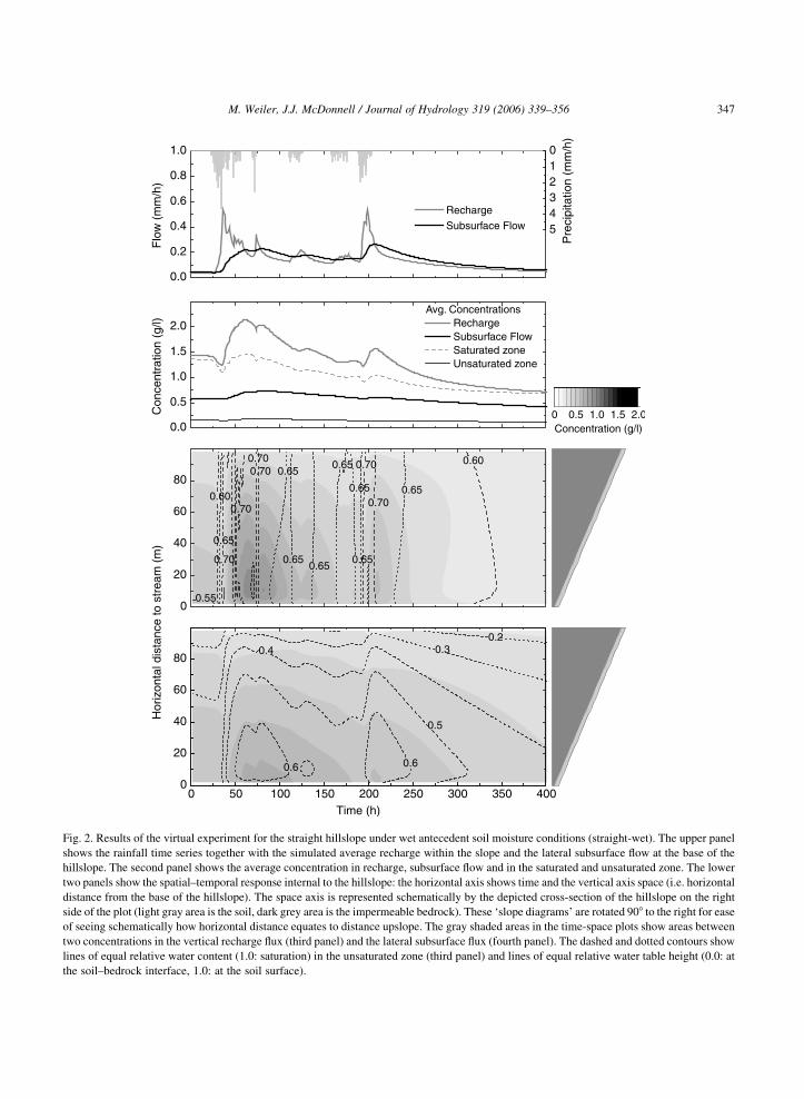
Fig. 2. Results of the virtual experiment for the straight hillslope under wet antecedent soil moisture conditions (straight-wet). The upper panel



two panels show the spatial–temporal response internal to the hillslope: the horizontal axis shows time and the vertical axis space (i.e. horizontal

distance from the base of the hillslope). The space axis is represented schematically by the depicted cross-section of the hillslope on the right








straight-dry experiment. Concentration in subsurface

flow is a somehow smoothed picture of the spatial–

temporal concentration pattern in recharge.

The results for the experiment with a concave

hillslope under dry antecedent soil moisture con-

ditions (concave-dry) are shown in Fig. 3. The

recharge and subsurface flow response in the upper

panel is quite similar to the response of the straight-

dry experiment. However, the concentration response

is quite different compared to the straight-dry

experiment with a more pronounced response of the

concentration in recharge as well as a higher

concentration in subsurface flow. One can observe

the influence of the concave hillslope profile in the

spatial-temporal plots of the lower two panels. Water

content response is higher in the lower, flatter part of

the hillslope than in the upper steeper part. This

response appears to directly influence the concen-

tration response in the recharge (third panel). A high

concentration is observed in the lower part of the

hillslope during the events, especially for the later

rainfall events in the time series. These higher

concentration peaks appear to control the concen-

tration response of the subsurface flow (fourth panel).

Especially for the last event in the series, high

concentration of lateral subsurface flow can be seen

in the lower part of the hillslope. Water table response

is also higher in the lower part of the slope, analogous

to a riparian zone. In general, the spatial–temporal

patterns for the concave slope are more distinct and

pronounced compared to the more muted temporal

pattern of the straight slopes.

We show the results of the fourth experiment at a

concave slope under wet antecedent soil moisture

conditions in Fig. 4. The first rainfall events result in

high recharge (upper panel in Fig. 4) and an associated

high mobilization in the unsaturated zone and

concomitant high concentration in recharge (second

panel). While the lateral subsurface flow response is

much more delayed compared to these 1D changes, it

is high compared to the previous three experiments. In

particular, the subsurface flow concentration response

peak at 80 h is much higher than any of the previous

observations.

The spatial–temporal plots in Fig. 4 reflect the

averaged result for the hillslope. Water content

response in the unsaturated zone is large for the first

event and is followed by very high concentrations in

recharge in the lower part of the hillslope. This high

level of mobilization results in very low concen-

trations in recharge in the lower part of the slope later

in the experiment due to the resulting depletion of the

unsaturated zone tracer store. The water table

response (shown in the fourth panel of Fig. 4) is

rapid and pronounced—so much so that we see the

lower part of the hillslope close to saturation for the

first time. Coincident with this are high concentrations

in the subsurface flow within the lower part of the

hillslope. As per the previous experiments, slope-wide

spatial variations of water table, water content and

concentration responses are quite marked.

3.2. Concentration–discharge relationship

Concentration–discharge relationships (C–Q-

plots) are a well established tool to analyze nutrient

behavior in watersheds in relation to streamflow

response (Bishop et al., 2004). We apply this method

to analyze the results of the four virtual experiments.

When plotting the C–Q relationships for one or

several rainfall–runoff events, hysteresis is commonly

observed since flow response and nutrient response

are frequently out of sync. The hysteresis is

commonly described by its direction of rotation:

clockwise and counterclockwise. If one considers the

probable hysteresis direction for the two different

flushing hypotheses posed earlier in this paper, we

may expect a clockwise direction for the transmissiv-

ity feedback flushing and a counterclockwise direc-

tion for the flushing by the vertical-lateral preferential

flow conceptual model.

Fig. 5 shows the C–Q relationships for the four

experiments. The color coding reflects time and thus

the direction of the looping. For the straight-dry

experiment, the relationship is quite tight and a

counterclockwise loop was detected. The straight-wet

experiment shows a more complex behavior: the first

rainfall events produce a counterclockwise loop,

followed by a very narrow loop through successive

rain inputs. Notwithstanding these complexities, the

overall relationship follows a clockwise loop. For the

concave-dry experiment, the simulations produce a

overall clockwise loop including a small clockwise

loop during the last storm. The C–Q relationships is

tighter compared to the straight-wet experiment,

however, the reader should note that the scale of

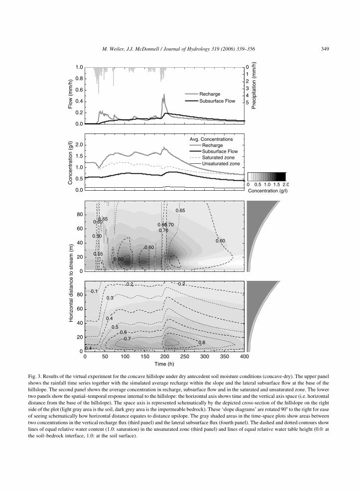
Fig. 3. Results of the virtual experiment for the concave hillslope under dry antecedent soil moisture conditions (concave-dry). The upper panel











Fig. 4. Results of the virtual experiment for the concave hillslope under wet antecedent soil moisture conditions (concave-wet). The upper panel











Fig. 5. Concentration–discharge plots for the four virtual experiments. Lines are color coded to show where on the hydrograph these hysteresis

loops relate. Note the directional changes in looping behavior and differences in loop amplitude, as explained in the text.


the vertical axis in Fig. 5 is different to enable

comparison of this experiment to the results of the

concave-wet experiment. These results, shown in the

lower right corner of Fig. 5, reveal a very wide

clockwise hysteresis including some smaller clock-

wise loops.

Fig. 6. Cumulative mass flux from recharge flow and water table

variations for the four virtual experiments.

3.3. First-order controls of nutrient export

We calculated the solute mass export mobilized

by vertical flow (i.e. recharge, computed via Eq. (4))

and by water table variations (computed via Eqs. (6)

and (7)). Fig. 6 shows the time series of solute

export by recharge and water table variations for the

four experiments. For the whole simulation period,

export by recharge is higher than export by water

table variations. Notwithstanding, during the first


100 h and hence the first two major rainfall events,

export by water table variations is larger for the

experiments with a concave slope profile. Since

recharge is a more continuous process as compared

to the episodic dynamics of the water table, export

by recharge is more continuous than export by water

table variations. In general, the higher the water

table rise (see, for example, the first event (between

40 and 70 h) for the experiments under wet initial

conditions) the greater the solute export. If one

ranks the export mass for the different experiments

and by different mobilization processes, the exper-

iment with wet antecedent conditions export more

mass by recharge than the experiments under dry

antecedent conditions. For export by water table

variations, experiments for concave slope profiles

show a higher total mass flux than for experiments

with straight slopes.

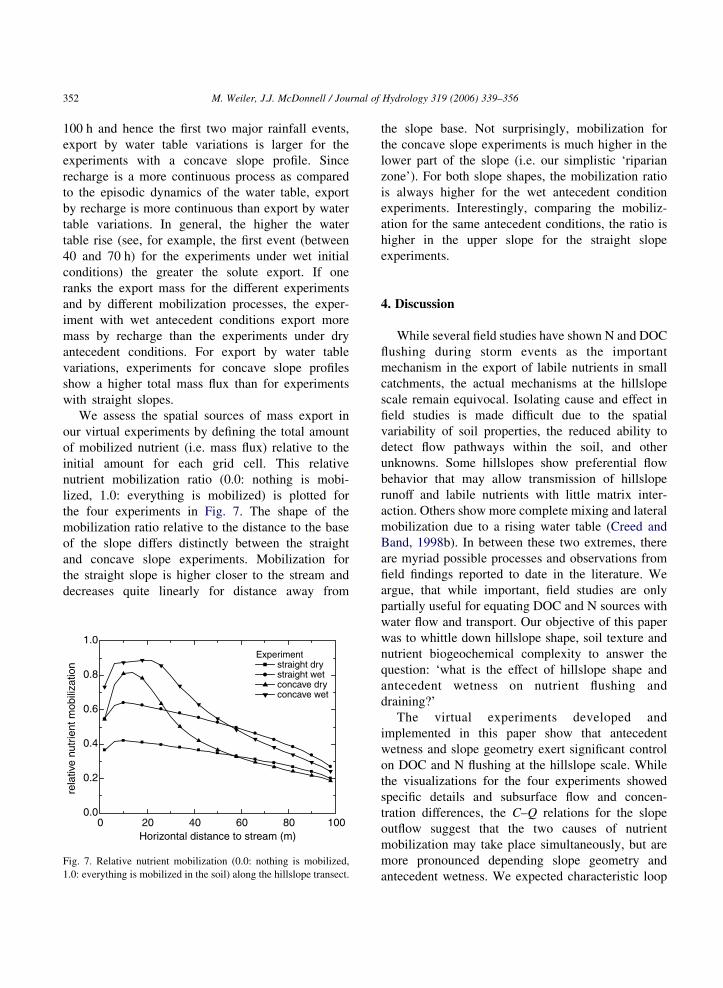
We assess the spatial sources of mass export in

our virtual experiments by defining the total amount

of mobilized nutrient (i.e. mass flux) relative to the

initial amount for each grid cell. This relative

nutrient mobilization ratio (0.0: nothing is mobi-

lized, 1.0: everything is mobilized) is plotted for

the four experiments in Fig. 7. The shape of the

mobilization ratio relative to the distance to the base

of the slope differs distinctly between the straight

and concave slope experiments. Mobilization for

the straight slope is higher closer to the stream and

decreases quite linearly for distance away from

Fig. 7. Relative nutrient mobilization (0.0: nothing is mobilized,

1.0: everything is mobilized in the soil) along the hillslope transect.

the slope base. Not surprisingly, mobilization for

the concave slope experiments is much higher in the

lower part of the slope (i.e. our simplistic ‘riparian

zone’). For both slope shapes, the mobilization ratio

is always higher for the wet antecedent condition

experiments. Interestingly, comparing the mobiliz-

ation for the same antecedent conditions, the ratio is

higher in the upper slope for the straight slope

experiments.

4. Discussion

While several field studies have shown N and DOC

flushing during storm events as the important

mechanism in the export of labile nutrients in small

catchments, the actual mechanisms at the hillslope

scale remain equivocal. Isolating cause and effect in

field studies is made difficult due to the spatial

variability of soil properties, the reduced ability to

detect flow pathways within the soil, and other

unknowns. Some hillslopes show preferential flow

behavior that may allow transmission of hillslope

runoff and labile nutrients with little matrix inter-

action. Others show more complete mixing and lateral

mobilization due to a rising water table (Creed and

Band, 1998b). In between these two extremes, there

are myriad possible processes and observations from

field findings reported to date in the literature. We

argue, that while important, field studies are only

partially useful for equating DOC and N sources with

water flow and transport. Our objective of this paper

was to whittle down hillslope shape, soil texture and

nutrient biogeochemical complexity to answer the

question: ‘what is the effect of hillslope shape and

antecedent wetness on nutrient flushing and

draining?’

The virtual experiments developed and

implemented in this paper show that antecedent

wetness and slope geometry exert significant control

on DOC and N flushing at the hillslope scale. While

the visualizations for the four experiments showed

specific details and subsurface flow and concen-

tration differences, the C–Q relations for the slope

outflow suggest that the two causes of nutrient

mobilization may take place simultaneously, but are

more pronounced depending slope geometry and

antecedent wetness. We expected characteristic loop


directions to be clockwise for the transmissivity

feedback flushing process and counter-clockwise for

the vertical to lateral bypass process. Our virtual

experiment results suggest that the transmissivity

feedback flushing process is more important for the

concave slopes than for the straight slopes.

Furthermore, we would conclude that the transmis-

sivity feedback hypothesis is more important under

wet than under dry antecedent moisture conditions.

To test these assertions, we then analyzed for the

origin of the nutrient mobilization by evaluating the

influence of the two different flushing hypotheses on

nutrient mass export from the hillslope. These

results showed that the transmissivity feedback

flushing process is more important for the concave

slopes than for the straight slopes and more

important under wet than under dry antecedent

moisture conditions. In addition, higher mobilization

for the wet antecedent conditions is supported by

higher mobilization due to recharge compared to the

dryer antecedent conditions.

4.1. The effect of a riparian zone

Following their hypothesis of riparian areas as

source areas of nitrate, McGlynn and McDonnell

(2003) further proposed that the catchment’s

N-flushing response would be strongly regulated

by how, where, and at what rate these riparian areas

function in the catchment. McGlynn and McDonnell

(2003) hypothesized that the rate of change of

riparian saturation and not the total riparian width

would be the key determinant in a catchment’s N

flushing response. We found that the riparian zone

(the lower part in the concave slopes) is the primary

source of nutrient mobilization even though we

assumed a constant initial concentration of nutrients

in the hillslope. The greater flow dynamics, water

table response and water content change in the

riparian zone amplifies nutrient mobilization

compared to a hillslope without riparian zone.

Thus the rate of change of riparian saturation that

we explore in our model may be a key factor as it

may be a surrogate for the dynamics in the riparian

zone. However, the upper slope still mobilized

nutrients that are transported to the stream (for our

set-up). This behavior may change when the volume

of the riparian zone is larger (e.g. deeper soils,

larger riparian zone width) and the mixing ratio

between the hillslope water with the riparian water

is larger. This is consistent with recent experimental

work of Creed and Band (1998b). They showed that

during a storm event, the proportion of riparian

runoff was larger on the rising than falling limb of

the hydrograph while the proportion of hillslope

runoff was smaller on the rising than falling limb of

the hydrograph. The delayed response of hillslope

runoff resulted in a disconnection between hillslope

and riparian areas early in the event and higher

DOC concentrations on the rising limb than the

falling limb of the event hydrograph. Later in the

event, Creed and Band (1998b) showed that

hillslope and riparian areas became connected once

the hillslope soil moisture deficits were satisfied.

They suggested that the relative timing of riparian

and hillslope source contributions, and the connec-

tions and disconnections of dominant runoff con-

tributing areas were the first-order catchment

controls on stream DOC concentrations and mass

export.

In general, the spatial distribution of riparian areas

in the catchment and their connectedness with the

stream network will be a key for delivery of nutrients

and thus regulate the nutrient flushing response.

Although Creed and Band (1998b) had observed

riparian areas as nitrate sources in their catchment,

they acknowledged that riparian zones could also be

potential N sinks due to processes like denitrification

and thus complicate the relationship between riparian

area response and the catchment N flushing response

(Creed et al., 1996; Worrall and Burt, 1999). These

effects remain to be explored in our virtual

experiments.

4.2. On the role of virtual experiments for facilitating

a dialog between hydrologist and biogeochemist

We argue that rather than a systematic examin-

ation of the first-order physical hydrological

controls on nutrient flushing at the hillslope and

catchment scale, field hydro-biogeochemical studies

have become mired in complexity. This has made it

difficult to intercompare different field sites and to

draw out common process behavior that may exist.

Even when major hillslope experiments and

excavations are undertaken to equate flushing


mechanisms with labile nutrient response

and export (e.g. Buttle et al., 2001), their results

are rarely transportable to other catchments. While

many useful individual experimental hillslope and

catchment investigations of nutrient flushing have

been completed recently (Bishop et al., 2004;

McGlynn and McDonnell, 2003), we still lack a

quantitative framework in which to test and

compare first-order controls on water and tracer

mass flux at this scale.

This paper has attempted to improve conceptu-

alization of labile nutrient flushing at the hillslope

scale by quantifying the interaction between water

flow pathways, source, and mixing at the hillslope

scale within a virtual experiment framework. These

numerical experiments with a model, driven by

collective field intelligence, are fundamentally

different to traditional numerical experiments since

the intent is to explore first-order controls in

hillslope hydrology and biogeochemical coupling

where the experimentalist and modeler work

together to collectively develop and analyze the

results. In addition to the traditional scalar output,

visualization has been a key interpretive part of the

approach. As in our previous virtual experiment

applications (Weiler and McDonnell, 2004), our

work is motivated by frustrations that we have had

personally in experiments at various hillslopes

where first-order effects on flushing often seem

difficult to separate from second and third order

effects. The work has been further motivated by

our general philosophy that hillslope models should

be simple, with few ‘tunable parameters’, and

might serve ultimately as useful hypothesis testing

tools. We have shown in this paper how one can

test a number of hypotheses within a virtual

experimental framework to inform a new organiz-

ational structure for labile nutrient flushing at the

hillslope scale.

Finally, this paper has taken a decidedly hydro-

centric view of nutrient flushing. Future experiments

might take a more biogeo-centric view whereby

production, mineralization, etc., are examined on the

timescale of events and seasonally to better under-

stand complex biogeochmical cycling within a

hydrological context. We hope that ultimately,

intercomparison and classification of field exper-

iments and development of hydrobiogeochical

catchment typologies may become common—leading

to new approaches in watersheds.

5. Conclusion

The delivery mechanisms of labile nutrients (e.g.

NO3, DON and DOC) to streams are poorly under-

stood. While several studies have shown N and C

flushing during storm events as the important

mechanism in the export of DOC and DON in small

catchments, the actual mechanisms at the hillslope

scale have remained equivocal. The difficulty in

isolating cause and effect in field studies is made

difficult due to the spatial variability of soil properties,

the reduced ability to detect flow pathways within the

soil, and other unknowns. The virtual experiments

described in this paper have focused on quantifying

the first-order controls on flow pathways and nutrient

transport in hillslopes. These virtual experiments

(numerical experiments with a model driven by

collective field intelligence) used a new distributed

model that describes the lateral saturated and vertical

unsaturated water flow from hypothetical finite and

infinite nutrient sources in the upper soil horizons. We

have shown how depth distributions of transmissivity

and drainable porosity, soil depth variability, as well

as mass exchange between the saturated and

unsaturated zone influence the mobilization, flushing

and release of labile nutrients at the hillslope scale.

Specifically, we found that: (1) the transmissivity

feedback flushing process is more important for the

concave slopes than for the straight slopes, (2)

transmissivity feedback is more important under wet

than under dry antecedent moisture conditions and (3)

the riparian zone (the lower part our virtual concave

slope) is the primary source of nutrient mobilization

even though we assumed a constant initial concen-

tration of nutrients over the entire hillslope. The

greater flow dynamics, water table response and water

content change in the riparian zone amplifies nutrient

mobilization compared to a (straight) hillslope with-

out riparian zone. Finally, while not a replacement for

field work, we argue that this new virtual experiment

approach provides a well-founded basis for defining

the first-order controls and linkages between hydrol-

ogy and biogeochemistry at the hillslope scale.


References

Anderson, M.G., Burt, T.P., 1982. The contribution of throughflow

to storm runoff: an evaluation of a chemical mixing model.

Earth Surface Processes and Landforms 33 (1), 211–225.

Anderson, S.P., Dietrich, W.E., Torres, R., Montgomery, D.R.,

Loague, K., 1997. Concentration-discharge relationships in

runoff from a steep, unchanneled catchment. Water Resources

Research 33 (1), 211–225.

Bear, J., 1972. Dynamics of Fluids in Porous Media. American

Elsevier Pub. Co., New York p. 764.

Bishop, K., Seibert, J., Kohler, S., Laudon, H., 2004. Resolving the

double paradox of rapidly mobilized old water with highly

variable responses in runoff chemistry. Hydrological Processes

18 (1), 185–189.

Boyer, E.W., Hornberger, G.M., Bencala, K.E., McKnight, D.M.,

1997. Response characteristics of DOC flushing in an alpine

catchment. Hydrological Processes 11 (12), 1635–1647.

Brown, V.A., McDonnell, J.J., Burns, D.A., Kendall, C., 1999. The

role of event water, a rapid shallow flow component, and

catchment size in summer stormflow. Journal of Hydrology 217,

171–190.

Burns, D.A., et al., 1998. Base cation concentrations in subsurface

flow from a forested hillsope: the role of flushing frequency.

Water Resources Research 34 (12), 3535–3544.

Buttle, J.M., Lister, S.W., Hill, A.R., 2001. Controls on runoff

components on a forested slope and implications for N transport.

Hydrological Processes 15, 1065–1070.

Creed, I.F., Band, L.E., 1998a. Exploring functional similarity in the

export of nitrate-N from forested catchments: a mechanistic

modeling approach. Water Resources Research 34 (11),

3079–3093.

Creed, I.F., Band, L.E., 1998b. Export of nitrogen from catchments

within a temperate forest: evidence for a unifying mechanism

regulated by variable source area dynamics. Water Resources

Research 34 (11), 3105–3120.

Creed, I.F., et al., 1996. Regulation of nitrate-N release from

temperate forests: a test of the N flushing hypothesis. Water

Resouces Research 32, 3337–3354.

Evans, C., Davies, T.D., 1998. Causes of concentration/discharge

hysteresis and its potential as a tool for analysis of episode

hydrochemistry. Water Resources Research 34 (1), 129–137.

Hagedorn, F., Bucher, J.B., Schleppi, P., 2001. Contrasting

dynamics of dissolved inorganic and organic nitrogen in soil

and surface waters of forested catchments with gleysols.

Geoderma 100, 173–192.

Hall, F.R., 1970. Dissolved solids-discharge relationships. Water

Resources Research 6 (3), 845–850.

Hangen, E., Lindenlaub, M., Leibundgut, C., von Wilpert, K.,

2001. Investigating mechanisms of stormflow generation by

natural tracers and hydrometric data: a small catchment study

in the Black Forest, Germany. Hydrological Processes 15,

183–199.

Hill, A.R., Kemp, W.A., Buttle, J.M., Goodyear, D., 1999. Nitrogen

chemistry of subsurface storm runoff on forested canadian

shield hillslopes. Water Resources Research 35, 811–821.

Hinton, M.J., Schiff, S.L., English, M.C., 1998. Sources and

flowpaths of dissolved organic carbon during storms in two

forested watersheds of the precambrian shield. Biogeochemistry

41, 175–197.

Hornberger, G.M., Bencala, K.E., McKnight, D.M., 1994. Hydro-

logical controls on dissolved organic carbon during snowmelt in

the Snake River near Montezuma, Colorado. Biogeochemistry

25 (3), 147–165.

Inamdar, S.P., Christopher, S. and Mitchell, M.J., 2004. Flushing

of DOC and nitrate from a forested catchment: Role of

hydrologic flow paths and water sources. Hydrological

Processes 18, 2651–2661.

Jemison Jr.., J.M., Fox, R.H., 1994. Nitrate leaching from nitrogen-

fertilized and manured corn measured with zero-tension pan

lysimeters. Journal of Environmental Quality 23 (2).

Lajtha, K. et al., 2004. Detrital controls on SOM dynamics and soil

solution chemistry: an experimental approach. Geoderma,

in press

Lawrence, G.B., Driscoll, C.T., 1990. Longitudinal patterns of

concentration-discharge relationships in stream water draining

the hubbard brook experimental forest. Journal of Hydrology

116, 147–165.

McGlynn, B.L., McDonnell, J.J., 2003. Role of discrete landscape

units in controlling catchment dissolved organic carbon

dynamics. Water Resources Research 39 (4).

10.1029/2002WR001525.

McHale, M.R., McDonnell, J.J., Mitchell, M.J., Cirmo, C.P., 2002.

A field-based study of soil water and groundwater nitrate release

in an adirondack forested watershed. Water Resouces Research

38 (4). 10.1029/2000WR000102.

Murdoch, P.S., Stoddard, J.L., 1992. The role of nitrate in the

acidification of streams in the Catskill Mountains of New York.

Water Resouces Research 28 (10), 2707–2720.

Pinder, G.F., Jones, J.F., 1969. Determination of the ground-water

component of peak discharge from the chemistry of total runoff.

Water Resources Research 5 (2), 438–445.

Qualls, R.G., Haines, B.L., 1991. Geochemistry of dissolved

organic nutrients in water percolating through a forest

ecosystem. Soil Science Society of American Journal 55,

1112–1123.

Ranken, D.W., 1974. Hydrologic properties of soil and subsoil on a

steep, forested slope. M.S. Thesis, Oregon State University,

Corvallis, p.114.

Rothacher, J., Dyrness, C.T. and Fredriksen, R.L., 1967. Hydrologic

and related characteristics of three small watersheds in the

Oregon Cascades, U.S. Department of Agriculture, Forest

Service, Pacific Northwest Forest and Range Experiment

Station, Portland, OR.

Tague, C.L., Band, L.E., 2001. Evaluating explicit and implicit

routing for watershed hydro-ecological models of forest

hydrology at the small catchment scale. Hydrological Processes

15, 1415–1440.

Tromp-van Meerveld, H.J., 2004. Hillslope hydrology: From

patterns to processes. Ph. D. dissertation, Oregon State

University, Corvallis, 270 pp.

Weiler, M., 2001. Mechanisms controlling macropore flow during

infiltration—dye tracer experiments and simulations. ETHZ,

urich, Switzerland p. 151.


Weiler, M., McDonnell, J.J., 2004. Virtual experiments: a new

approach for improving process conceptualization in hillslope

hydrology. Journal of Hydrology 285, 3–18.

Weiler, M. and McDonnell, J.J., 2005. Virtual isotope hydrograph

separation: Examining the effects of pre-event water variability

on estimated runoff components. Journal of Hydrology, in

review.

Welsch, D.L., Kroll, C.N., McDonnell, J.J., Burns, D.A., 2001.

Topographic controls on the chemistry of subsurface stormflow.

Hydrological Processes 15, 1925–1938.

Weyman, D.R., 1973. Measurements of the downslope flow of

water in a soil. Journal of Hydrology 20, 267–288.

Wigmosta, M.S., Lettenmaier, D.P., 1999. A comparison of

simplified methods for routing topographically driven subsur-

face flow. Water Resources Research 35, 255–264.

Wigmosta, M.S., Vail, L.W., Lettenmaier, D.P., 1994. A distributed

hydrology-vegetation model for complex terrain. Water

Resources Research 30 (6), 1665–1679.

Worrall, F., Burt, T.P., 1999. The impact of land-use change on

water quality at the catchment scale: the use of export coefficient

and structural models. Journal of Hydrology 221 (1–2), 75–90.

Yee, C.S., Harr, R.D., 1977. Influence of soil aggregation on slope

stability in the oregon coast ranges. Environmental Geology and

Water Sciences 1 (6), 367–377.

testing nutrient ﬂushing hypotheses at the hillslope scale

Documents