testing intertemporal models of the current … · testing intertemporal models of the current...

Testing Intertemporal Models of the

Current Account for Australia

King Pong Tam

Bachelor of Commerce

(Honours in Business Economics)

The University of New South Wales

6 June 2008

1

Declaration

I hereby declare that this thesis is my original work and citations of other authors have been

properly referenced in the text. This thesis contains no material which has been submitted to

any other institutions as part of the requirements for a degree or other award.

King Pong Tam

6 June 2008

2

Acknowledgements

I would like to express my gratefulness to have the guidance and support from my supervisor

Glenn Otto throughout the Honours year. His extensive economics knowledge has deeply

inspired my passion towards macroeconomics and this thesis would not be possible without

his generous assistance. I also wish to thank Garry Barrett and Lance Fisher who kindly

offered me advice and suggestions on my econometrics methods. I am thankful to those

present at my final thesis presentation and their helpful comments are highly appreciated.

I am grateful to be awarded with the scholarships from the Centre of Applied Economic

Research, the Australian School of Business and the University of New South Wales which

provided me great encouragement in my Honours year.

I would also like to thank my Honours fellows for their cheerful support. Thank you to my

girlfriend Wing Ng for her precious care and tremendous assistance. My special thanks to my

family and friends especially my mother and father for their invaluable love and

encouragement.

3

Abstract

This thesis investigates the ability of three versions of the intertemporal model of the current

account to account for fluctuations in Australia’s current account. The intertemporal

framework attributes an economy’s current account to the outcome of rational consumption

and investment decisions by various agents in the economy. The basic intertemporal model

emphasizes consumption smoothing as a determinant of the current account, with a key role

played by the expectation of the future changes in national cash flow. In a generalized version

of the intertemporal model due to Bergin and Sheffrin (2000), the current account does not

solely driven by the movements in net cash flow but also by the real exchange rate and world

real interest rate. Bergin and Sheffrin’s model is extended by Bouakez and Kano (2008) who

also incorporate a role for the terms of trade into the intertemporal model.

All of the intertemporal models considered give rise to a present-value relationship for the

current account. An implication of the models is that the current account should anticipate

and consequently forecast the forcing variables. Using the Granger-causality tests and long

horizon tests, it is found that Australia’s current account is able to forecast changes in net

cash flows over horizons of one to two years. However there is little support for any

relationship between the current account and other variables implied by either of the

generalized models. A formal (orthogonality) test of the basic model indicates that it is not

rejected by the Australian data. Interestingly, no improvement is found for the fit of the

intertemporal model in the financial deregulated environment from 1980 and this differs from

previous findings (Cashin and McDermott, 1998)

4

Table of Contents

Declaration ................................................................................................................................. 1

Acknowledgements .................................................................................................................... 2

Abstract ...................................................................................................................................... 3

Chapter 1: Introduction ................................................................................................................. 8

Chapter 2: Intertemporal Models of the Current Account ...................................................... 15

2.1 Basic Intertemporal Model of the Current Account ................................................................. 15

2.2 Generalized Intertemporal Model of the Current Account ...................................................... 18

2.3 Extension of the Intertemporal Model for the Current Account .............................................. 23

Chapter 3: Data ............................................................................................................................ 31

3.1 Data Sources ............................................................................................................................ 31

3.2 Construction of Variables ........................................................................................................ 31

3.3 Unit Root Tests ........................................................................................................................ 34

Chapter 4: Tests of the Intertemporal Models .......................................................................... 37

4.1 Granger-causality Tests ........................................................................................................... 37

4.2 Long Horizon Regressions ....................................................................................................... 38

4.3 Orthogonality Tests .................................................................................................................. 39

4.4 Results ...................................................................................................................................... 42

Full sample Result ...................................................................................................... 42

Sub-samples Results ................................................................................................... 47

Chapter 5: Conclusion ................................................................................................................. 60

5

Appendix A: Data Set ....................................................................................................................... 64

Appendix B: Graphs of the Main Variables ..................................................................................... 66

Bibliography ......................................................................................................................................... 69

6

Lists of Figures

Figure 1: Australia’s Current Account as a Share of GDP

Figure 2: Australia’s Current Account Series (1960-2007)

Figure 3: Australia’s Movements in National Cash Flow Series (1960-2007)

Figure 4: World Real Interest Rate Series (1960-2007)

Figure 5: Australia’s Movements in Real Exchange Rate Series (1960-2007)

Figure 6: Australia’s Consumption-based Interest Rate Series (1960-2007)

Figure 7: Australia’s Terms of Trade Variations Series (1960-2007)

7

Lists of Tables

Full Sample (1960 – 2007)

Table 1: Unit Root Tests

Table 2: Granger-Causality Tests of the Intertemporal Models for Australia

Table 3: Long Horizon Tests of the Intertemporal Models for Australia

Table 4: Orthogonality Tests of the Intertemporal Models for Australia

Sub-Sample (1960 – 1980)




Sub-Sample (1981 – 2007)




8

Chapter 1: Introduction

Australia has traditionally been a capital importing country with a long history of large

current account deficits. The sizeable and persistent current account deficits were frequently

raised as a cause of concern in the 1980s, due to their possible adverse effect on the domestic

economy. Countries with large and persistent current account deficits are sometimes

considered to be on a path of insolvency which may eventually increase the chances of a

significant reversal in capital flows and prospects of default. Current account deficits are also

the originator of foreign indebtedness and thus the major influence on the size of external

debts. The rising indebtedness and large current account deficits may leave countries

vulnerable to external shocks if foreign lenders change their willingness to lend for external

debts (Pitchford, 1990). However, Australia has no experience of default on public debt and

there have not been any significant reversal in capital flows.

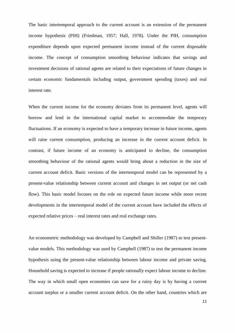
Figure 1 shows the annual current account as a share of nominal gross domestic product

(GDP) from 1960 to 2007. From the mid 1960s to early 1970s, Australia experienced an

investment boom in resources-related industries. It stimulated the Australian economy by

having a real income growth with average of 5 per cent per annum. The increased investment

in the early stages of the boom contributed to the raised current account deficit which implied

the involvement of imported capital in the investment boom. The speculation of devaluation

under the managed exchange rate regime in the late 1970s and early 1980s and the pressure

for a complete liberalization of the capital account eventually led to the development of a

floating exchange rate regime in December 1983. The depreciation of the Australian dollar

that followed immediately after the floating of exchange rate improved the international

competitiveness of domestic firms.

9

The increase in the current account deficit from an average of 4% of GDP in the early 1980s

to figures in the range of 4% to 7% in the late 1980s attracted the attention of many

government authorities, economic commentators and academics. The removal of capital

controls and the development of the floating exchange rate regime allow foreigners to freely

invest in Australia and produced an inflow of foreign capital. Australia’s current account

deficit was viewed as a serious problem in the latter part of the 1980s which required a

remedial policy action. In the late 1990s when the technology boom emerged, Australia was

viewed as a traditional economy which contributed to a large depreciation of Australian

dollar. This improved the trade balance and the associated current account deficit in Australia.

The overall size and level of fluctuations in the current account deficit also declined since the

latter part of 1990s compared to the late 1980s.

-8.00%

-7.00%

-6.00%

-5.00%

-4.00%

-3.00%

-2.00%

-1.00%

0.00%

1.00%

2.00%

3.00%

19

60

19

62

19

64

19

66

19

68

19

70

19

72

19

74

19

76

19

78

19

80

19

82

19

84

19

86

19

88

19

90

19

92

19

94

19

96

19

98

20

00

20

02

20

04

20

06

20

08

Figure 1 Australia's Current Account as a Share of GDPProportion of

GDP

YearSource: Australian Bureau of Statistics

10

Apart from the trend-decline in the size of the current account deficit since the 1980s, the

emergence of the Pitchford’s (1990) argument and the intertemporal approach of the current

account have significantly changed the way in which policy-makers and economists think

about the current account. From the early 1970s to December 1983, prior to the floating

exchange rate regime, Australia’s current account deficit was a concern for policy makers. To

the extent that the deficit was not matched by the capital flows it was required to be financed

by reducing foreign exchange reserve. After the float of the Australian dollar, the view that

current account balance should be regarded as a policy target persisted and there were

increased concerns about the persistent and sizeable deficits in the mid 1980s. The current

account deficit and the associated external debt were viewed as major policy issues and

intervention was considered to be necessary to rein in the large current account deficits.

By the end of 1980s, the view that current account is basically the outcome of rational

decisions by private agents was propounded by several Australian academics (Pitchford,

1990). Policy intervention to reduce the deficit was considered under this view to be

unnecessary and may even reduce social welfare. The relevance of having the current account

as an explicit goal for the monetary policy was also debated within the Reserve Bank of

Australia. The development of models which focus on the intertemporal character of current

account over the previous decade also contributed to the change of perception on current

account (Frenkel and Razin, 1987; Obstfeld and Rogoff, 1996). In the Australian context, the

intertemporal approach to the current account is most closely associated with Pitchford’s

(1990) argument. It is now widely accepted that current account balance should not be a

policy objective, at least to the extent that it reflects the optimal decisions of borrowers and

lenders.

11

The basic intertemporal approach to the current account is an extension of the permanent

income hypothesis (PIH) (Friedman, 1957; Hall, 1978). Under the PIH, consumption

expenditure depends upon expected permanent income instead of the current disposable

income. The concept of consumption smoothing behaviour indicates that savings and

investment decisions of rational agents are related to their expectations of future changes in

certain economic fundamentals including output, government spending (taxes) and real

interest rate.

When the current income for the economy deviates from its permanent level, agents will

borrow and lend in the international capital market to accommodate the temporary

fluctuations. If an economy is expected to have a temporary increase in future income, agents

will raise current consumption, producing an increase in the current account deficit. In

contrast, if future income of an economy is anticipated to decline, the consumption

smoothing behaviour of the rational agents would bring about a reduction in the size of

current account deficit. Basic versions of the intertemporal model can be represented by a

present-value relationship between current account and changes in net output (or net cash

flow). This basic model focuses on the role on expected future income while more recent

developments in the intertemporal model of the current account have included the effects of

expected relative prices – real interest rates and real exchange rates.

An econometric methodology was developed by Campbell and Shiller (1987) to test present-

value models. This methodology was used by Campbell (1987) to test the permanent income

hypothesis using the present-value relationship between labour income and private saving.

Household saving is expected to increase if people rationally expect labour income to decline.

The way in which small open economies can save for a rainy day is by having a current

account surplus or a smaller current account deficit. On the other hand, countries which are

12

optimistic towards future income prospects will tend to run a current account deficit or a

smaller current account surplus.

A number of empirical studies have been conducted to test the intertemporal approach to the

current account, following Campbell’s (1987) method. There are various degrees of formal

statistical support for the intertemporal approach. In an early study for Australia, Milbourne

and Otto (1992) rejected the restrictions of the basic intertemporal model using quarterly data.

The intertemporal approach was also tested by Cashin and McDermott (1998, 2002) and the

basic intertemporal model was strongly rejected. The consumption smoothing model of the

current account was found to be a poor approach to explaining Australia’s current account

behaviour. More recently Otto (2003), however, suggested that the intertemporal model was

able to explain the annual changes in Australia’s current account deficit for the sample dated

from 1980 to 2003.

The basic model in most of the existing studies is statistically rejected for many small open

economies (Obstfeld and Rogoff, 1995). In response, economists sort to include other

variables into the simple intertemporal model and the generalized intertemporal model was

developed. The generalized intertemporal approach allows for small open economies to be

affected by a number of external shocks. These include changes in the world real interest rate

and the real exchange rate. When facing changes in world real interest rate, economic agents

are influenced in how they allocate their consumption expenditure towards the present or the

future. Thus countries will choose to increase or decrease their current account balance in

respond to changes in the interest rate or exchange rate (Bergin and Sheffrin, 2000). There is

some evidence that Bergin and Sheffrin’s generalized intertemporal model provides a better

description of Australia’s current account than does the basic model. .

13

A recent extension of the intertemporal model allows for changes in the terms of trade. The

inclusion of this variable seeks to account for the Harberger-Laursen-Metzler (HLM) effect,

where a temporary rise in terms of trade tends to improve the current account. Bouakez and

Kano (2008) develop an intertemporal model of current account which accounts for the HLM

effect in addition to the traditional consumption smoothing behaviour and the effects of

future changes in exchange rate and time varying interest rate, as highlighted in Bergin and

Sheffrin. The extended intertemporal model illustrates not only the intertemporal substitution

effect but also the income and wealth effects with a change in the world interest rate and the

immediate effect on net foreign interest payments.

The empirical work by Bouakez and Kano finds the generalized intertemporal model which

allows for variations in interest and exchange rate does not improve the fit of the standard

model on Australia’s data which contrasts to the results of Bergin and Sheffrin. Furthermore

their extended model, augmented with terms of trade variations, was strongly rejected by the

Australia’s data and variations in terms of trade did not seem to significantly affect the

current account.

There is mixed evidence about the ability of the intertemporal models to explain Australia’s

current account. The aim of this thesis is to examine and compare the ability of the models

(basic, generalized and extended) to explain fluctuations in Australia’s current account. In

particular it examines whether the inclusion of the world interest rate, the exchange rate and

the terms of trade yield an improvement in the fit of data.

14

The predictions of the intertemporal models are also tested using three methods: Granger-

Causality tests (Granger, 1969); long horizon regressions (Campbell and Shiller, 1988) and a

test of the orthogonality restrictions. The empirical models are estimated using annual data

over a full sample period 1960-2007 and two sub-sample periods 1960-1980 and 1980-2007.

Previous studies on Australian data suggest that there is stronger support for the models

during the post-deregulation period (Cashin and McDermott, 1998, 2002; Otto, 2003).

The results indicate that for the full sample period, allowing for a time-varying real interest

rate, the real exchange rate and the terms of trade does not generate any improvement in the

model to fit the data. The basic intertemporal model seems to provide the best explanation of

the Australian data. Using the data for the two sub-samples; the generalized intertemporal

model is rejected for both periods, while there is some support for the extended intertemporal

model during the later sub-sample period.

The rest of the thesis is structured as follows. Chapter 2 outlines the various intertemporal

models of the current account. Chapter 3 describes the data including; data sources,

construction of variables, choice of parameter values and results of unit root tests. Chapter 4

discusses the methods used to examine the predictions of the models and reports the results

from testing the models on the Australian data. Chapter 5 concludes.

15

Chapter 2: Intertemporal Models of the Current Account

2.1 Basic Intertemporal Model for the Current Account

The basic intertemporal model considers an infinitely lived representative household in a

small open economy. The intertemporal model is similar to the permanent income hypothesis

(Friedman, 1957, Hall, 1978) where the representative agent chooses an optimal consumption

path to maximise the present-value of lifetime utility subject to a budget constraint. The

consumer’s expected lifetime utility function at period t is given as:

max E0 𝛽𝑡𝑈(𝐶𝑡

∞

𝑡=0

) 0 < 𝛽 < 1 (1)

where Ct is the consumption at period t, U(.) is the consumer’s period utility function and β is

the subjective discount factor with a value between 0 and 1. Et is the expectation operator

conditional upon the information set of period t.

The basic intertemporal model specifies the requirement of a small open economy. The real

interest rate for this economy is assumed to be constant over time and determined by the

international financial market. Regarding the above assumption, the consumption decision of

the agent can be made without reference to any production decision and only depends on a

country’s wealth (Sheffrin and Woo, 1990). It is also assumed that only a single good exists

in the small open economy (Sheffrin and Woo, 1990, Otto, 1992, Ghosh, 1995).

The agent’s consumption behaviour is subject to a budget constraint. By defining Bt as the

stock of net external assets at the beginning of period t. Yt is output, It is investment

16

expenditure and Gt is government spending. The consumer’s budget constraint is given as

follows:

𝑌𝑡 − 𝐶𝑡 − 𝐼𝑡 − 𝐺𝑡 + 𝑟𝐵𝑡−1 = 𝐵𝑡 − 𝐵𝑡−1 (2)

The last term on the left hand side of the budget constraint, rBt-1, equals to the interest earned

by the stock of net external assets held in the previous period. Additionally, the right hand

side of the budget constraint, Bt - Bt-1, equals to the change in the stock of net external assets

held from previous period to current period. Bt - Bt-1 is also equivalent to the current account

in current period. Thus, equation (2) can be represented in this form

𝑍𝑡 − 𝐶𝑡 + 𝑟𝐵𝑡−1 = 𝐶𝐴𝑡 , (3)

To obtain an optimal consumption path, the representative household has to maximize

equation (1) subject to constraint equation (2). The following Euler equation is obtained from

the first-order conditions of the optimization problem:

𝑢′ 𝐶𝑡 = 𝛽𝐸𝑡 1 + 𝑟 𝑢′ 𝐶𝑡+1 , 4

where 𝛽 = 1

1 + 𝑟

The following transversality condition is also imposed:

lim𝑖→∞

1

1 + 𝑟 𝑖

𝐵𝑡+𝑖 = 0 , 5

By summing the consumer’s budget constraint (2) over the infinite future and using the

transversality condition (4), the consumer’s intertemporal budget constraint is obtained where

the present value of consumption equals to the present value of net income and net external

assets in the initial period:

17

1

1 + 𝑟 𝑖+1

𝐶𝑡+𝑖 =

∞

𝑖=0

1

1 + 𝑟 𝑖+1

𝑍𝑡+𝑖 + 𝐵𝑡

∞

𝑖=0

, (6)

Assuming a quadratic form for the utility function and using the equations (4) and (6), the

following present-value model for the current account cat can be obtained (Obstfeld and

Rogoff, 1996):

𝐶𝐴𝑡 = −𝐸𝑡 𝛽𝑖∞

𝑖=1

∆𝑍𝑡+𝑖 (7)

Equation (7) shows that a country’s current account is equivalent to (minus) the present

discounted value of the infinite sum of expected future changes in national (net) cash flow, Zt.

This equation implies that a country will run a current account deficit if agents expect

changes in national cash flow to rise in the future and increase their current consumption. In

order to finance the temporary short-fall in current income, a country will smooth

consumption by borrowing in world capital markets and therefore running a current account

deficit. This mechanism is consistent with Campbell’s (1987) analogy where the permanent

income model can be illustrated by households’ decisions to save when the future labour

income is expected to decline. In the basic intertemporal model, net cash flow substitutes for

labour income and current account substitutes for saving. The current account has a major

function for consumption smoothing behaviour when the net cash flow is temporarily

deviated from its permanent level.

The basic intertemporal model also implies that current values of current account contain

information which is useful to forecast agents’ expectations of future changes in net cash

18

flows. Thus, the current value of current account is deemed to be a predicator of future

changes in national cash flows.

A number of previous empirical studies have found that the basic intertemporal model is

quite restrictive and fails for many small open economies. This result is surprising as it is

anticipated that the basic model to be most appropriate for small open economies where they

can borrow from the rest of the world without imposing any changes in variables such as the

equilibrium world interest rate.

However in light of these findings, a number of studies have sort to relax the assumption that

the world real interest rate is constant over time and only one good is produced in the

economy (which ignores the role of real exchange rate in affecting the current account).

Bergin and Sheffrin (2000) develop a generalized model in which current account depends

not only on net cash flow but also on the world real interest rate and country’s real exchange

rate.

2.2 Generalized Intertemporal Model for the Current Account

Bergin and Sheffrin (2000) extended the basic intertemporal model by assuming a small

country producing both traded and non-traded goods. The country can also borrow and lend

in the world capital market at a time-varying real interest rate. In the model, changes in both

real interest rate and real exchange rate stimulate consumption substitution between periods

and therefore it generates an intertemporal effect on a country’s current account. A

representative household chooses a consumption path that maximizes their discounted life

time utility:

19

max E0 𝛽𝑡∞

𝑡=0

𝑈 𝐶𝑇,𝑡 ,𝐶𝑁,𝑡 8

where 𝑈 𝐶𝑇,𝑡 ,𝐶𝑁,𝑡 =1

1 − 𝜍 (𝐶𝑇,𝑡

𝛼 𝐶𝑁,𝑡1−𝛼)1−𝜍

𝜍 > 0, 𝜍 ≠ 1, 0 < 𝜍 < 1

The functional form of the household’s utility is specified as above, where σ is equivalent to

the concavity of the utility function and α represents the share of traded goods in total

consumption. The utility function is assumed to exhibit the constant relative risk aversion.

Total consumption in the economy is now separated into consumption of traded goods, CT,t

and consumption of non-traded goods CN,t. The household utility maximization decision is

again subject to a budget constraint:

𝑌𝑡 − 𝐶𝑇,𝑡 + 𝑃𝑡𝐶𝑁,𝑡 − 𝐼𝑡 − 𝐺𝑡 + 𝑟𝑡𝐵𝑡−1 = 𝐵𝑡 − 𝐵𝑡−1 (9)

The relative price of non-traded to traded goods at time t is denoted Pt. It can be calculated as

PN,t divided by PT,t. Based on the assumption that the economy has both traded and non-

traded goods, the total consumption expenditure in terms of traded goods is equal to CT,t +

PtCN,t. Other variables in equation (9) are equivalent to those in equation (2) respectively. A

major difference between the budget constraint in basic and generalized model is that rt in

equation (9) represents the world real interest rate in terms of traded goods, which may be

time varying rather than a constant.

The right hand side of the budget constraint represents the current account in the present

period and thus equation (9) can be written as following:

𝑍𝑡 − 𝐶𝑡 + 𝑟𝐵𝑡−1 = 𝐶𝐴𝑡 (10)

20

The national cash flow Zt is defined as Yt – It – Gt. By summing up the budget constraint over

an infinite horizon and imposing the transversality condition:

lim𝑡 → ∞

E0(𝑅𝑡𝐵𝑡+𝑖) = 0 (11)

where 𝑅𝑖 = 1 (1 +

𝑖

𝑗=1

𝑟𝑗 )

the following intertemporal budget constraint is obtained (where B0 is the net foreign assets

in the initial period):

E0

∞

𝑖=0

𝑅𝑖𝐶𝑡+𝑖 = E0(𝑅𝑖𝑍𝑡+𝑖

∞

𝑖=0

) + 𝐵0 (12)

Based on the functional form of utility illustrated in equation (8), Bergin and Sheffrin (2000,

Appendix A) derived the first-order conditions for the problem of household utility

maximization and the optimal consumption profile can be defined as follow:

1 = E𝑡 𝛽𝛾(1+𝑟𝑡+1)𝛾 𝐶𝑡𝐶𝑡+1

𝑃𝑡𝑃𝑡+1

𝛾−1 1−𝛼

(13)

where γ is the intertemporal elasticity of substitution and equals to 1 / σ, which is the

reciprocal of the concavity of the utility function. Bergin and Sheffrin (2000) followed the

methodology adopted by Dornbusch (1983) and Obstfeld and Rogoff (1996) to derive the

optimal consumption profile in equation (13). This method involves specifying the Cobb-

Douglas consumption index with regards to the utility function and defining a related price

index. The intertemporal Euler equation is then constructed as equation (13) which is

expressed in terms of total consumption expenditure and the relative price of non-traded

goods.

21

By assuming joint log normality with constant variances and covariances, equation (13) can

be expressed in logs as follow:

E𝑡∆𝑐𝑡+1 = 𝛾E𝑡𝑟𝑡+1∗ 14

where 𝑟∗ = 𝑟𝑡 + 1 − 𝛾

𝛾(1 − 𝛼) ∆𝑝𝑡 + constant

∆𝑐𝑡+1 = log 𝐶𝑡 + 1 – log 𝐶𝑡 and ∆𝑝𝑡+1 = log 𝑃𝑡+1 – log 𝑃𝑡

The optimal consumption profile is thus influenced by the world varying interest rate, rt, and

the change in the relative price of non-traded goods, Δpt. Consumption based interest rate, r*

is then computed by integrating the above two variables. Movements in the consumption

based interest rate will affect households’ consumption decisions in the economy.

The main difference between basic intertemporal model and generalized intertemporal model

is the inclusion of consumption based interest rate (which is composed of time varying

interest rate and change in the relative price of non-traded goods). Considering the permanent

income hypothesis (Friedman, 1957, Hall, 1978), the basic intertemporal model proposes that

the agents’ consumption is subject to permanent income only where they borrow and lend

over time in the world financial market to smooth their consumption. The expected change in

consumption is thus zero. Contrary to the above proposition, the generalized intertemporal

model allows households to change their consumption profile when facing changes in terms

of borrowing and lending. The expected change in consumption is no longer zero in the

generalized model and the consumption smoothing behaviour will also be altered.

The intertemporal substitution of consumption can be analysed through the movements in

real interest rate and the changes in the relative price of non-traded goods. A rise of the

conventional interest rate, r, causes the current consumption to become more costly in terms

22

of future consumption forgone and thus creates an incentive for household to switch towards

future consumption with elasticity γ. An expected fall in the relative price of non-traded

goods can bring a similar intertemporal effect as above. The price of traded goods is therefore

expected to rise and it will cost more in future to repay the loan in traded goods in terms of

the consumption basket. Consumption based interest rate, r*, will be higher than the

conventional interest rate, r, and thus the current consumption will be decreased by elasticity

γ (1 – α).

The intratemporal substitution between traded and non-traded goods is also induced due to

the changes to their relative prices. Households will substitute towards traded goods by

intratemporal elasticity if the price of non-traded goods is temporarily high relative to traded

goods. The current consumption expenditure will then be raised by elasticity (1- α).

A present-value relationship for the current account is developed by using the optimal

consumption profile in equation (14) together with the intertemporal budget constraint in

equation (12). The present-value relationship for the current account in the generalized model

depends upon not only the national cash flow but also the consumption based interest rate.

Bergin and Sheffrin (2000) log linearised the intertemporal budget constraint in equation (12)

and assumed the net foreign assets are zero. The resulting present value relationship of the

current account is presented as follows in log terms:

𝑐𝑎𝑡∗ = −E𝑡 𝛽𝑖 ( ∆𝑧𝑡+𝑖

∞

𝑖=1

− 𝛾𝑟𝑡+𝑖∗ ) (15)

where 𝑐𝑎𝑡∗ ≡ 𝑛𝑜𝑡 − 𝑐𝑡

23

Comparing the present value relationship between basic and generalized models, the addition

of the consumption based interest rate in the generalized intertemporal model in equation (15)

is the major difference between the models. If net cash flow is expected to decrease in future

periods, the current account will increase due to the households’ consumption smoothing

behaviours. Apart from any changes in the expected national cash flow, an increase in the

consumption based interest rate will induce the agents in the economy to defer current

consumption. Thus, the current account will improve.

Bergin and Sheffrin (2000) indicated that an intertemporal model which allows for varying

interest rates and distinction between tradable and non-tradable goods substantially improves

the fit of the model over the basic intertemporal model. The modification of the basic model

helps the prediction of the model to fit the volatility of current account better and thus

improved the ability of the model to explain the current account fluctuations.

2.3 Extension of the Intertemporal Model for the Current Account

Bouakez and Kano (2008) developed an intertemporal model which has similar assumptions

as the generalized model above where representative households can consume both tradeable

and non-tradeable goods in a small open economy. Three kinds of goods (exportable goods,

importable goods and non-tradable goods) are now assumed to exist in the economy. In order

to measure the present-value relationship between variations in terms of trade and the current

account, a stochastic infinite horizon model have to be constructed with the following

household’s lifetime utility:

𝑈𝑡 = 𝐸𝑡 𝛽𝑖∞

𝑖=0

𝐶𝑡+𝑖1−1/𝜍

1 − 1/𝜍 , 0 < 𝛽 < 1, 𝜍 > 0, (16)

24

Similar notations as previous models have used; where β is the subjective discount factor and

σ is the elasticity of the intertemporal substitution. Et is the expectation operator conditional

on the information set available at time t. The consumption index, Ct, is a Cobb-Douglas

aggregator of tradeable goods and non-tradable goods as follow:

𝐶𝑡 = 𝜔1(𝐶𝑡𝑇)𝜖(𝐶𝑡

𝑁)1−𝜖 , 0 < 𝜖 < 1 , (17)

The total consumption expenditure is now separated in to 𝐶𝑡𝑇 and 𝐶𝑡

𝑁 which are consumption

of tradeable goods and consumption of non-tradeable goods respectively. represents the

weight of tradeable goods in the consumption bundle and 1

1 (1 ) is a positive

parameter. The price of tradable goods is then normalized to 1 (Bouakez and Kano, 2008)

and the consumption based price index, c

tP , is constructed as follow where the price of non-

tradable goods is denoted tQ :

𝑃𝑡𝑐 = 𝑄𝑡

1−𝜖 (18)

Obstfeld (1996) and Obstfeld and Rogoff (1996) defined the consumption of tradable goods

is a mix of exportable and imported goods in an economy. Assuming the tradeable good is

also a Cobb-Douglas aggregator of domestic exportable goods and domestic imported goods,

the tradable good consumption can be interpreted as follow,

𝐶𝑡𝑇 = 𝜔2𝑋𝑡

𝛾𝑀𝑡

1−𝛾 , 0 < 𝛾 < 1 , (19)

where the consumption of exportable goods and consumption of imported goods at period t

are denoted Xt and Mt respectively. Parameter 𝜔2 is positive and equals to 𝛾−𝛾(1 − 𝛾)𝛾−1.

25

Since the price of tradable goods is normalized to 1, the following condition regarding the

prices of domestic exportable goods, 𝑃𝑡𝑥 , and the price of imported goods, 𝑃𝑡

𝑚 , must hold:

1 = (𝑃𝑡𝑥)𝛾(𝑃𝑡

𝑚)1−𝛾 (20)

The terms of trade which is the price of export divided by the price of imports can then be

constructed as follow:

𝑃𝑡 = 𝑃𝑡𝑥

𝑃𝑡𝑚 − (𝑃𝑡

𝑥)1

1−𝛾 (21)

Suppose an economy with initial endowment of exportable and non-tradable net outputs at

the beginning of period t. The representative households then distribute the allocated income

to the consumption of exportable, non-tradable and imported goods. Part of the income is also

spent on purchasing the international bonds. Thus, the households have to face the following

budget constraint in each period:

𝐵𝑡+1 = 1 + 𝑟𝑡 𝐵𝑡 + 𝑃𝑡𝑥𝑁𝑌𝑡

𝑥 + 𝑄𝑡𝑁𝑌𝑡𝑛 − 𝑃𝑡

𝑐𝐶𝑡 (22)

where exportable net output is denoted by 𝑁𝑌𝑡𝑥 and non-tradable net output is denoted by

𝑁𝑌𝑡𝑛 . In order to maximize household’s lifetime utility function in equation (16) subject to

the budget constraint in equation (22) where a Ponzi scheme is not allowed, the first order

condition of this problem yields the following Euler equation:

1 = 𝛽𝐸𝑡 1 + 𝑟𝑡+1 𝑃𝑡𝑐

𝑃𝑡+1𝑐

𝐶𝑡𝐶𝑡+1

1/𝜍

(23)

By imposing the following transversality condition on international bond holdings where Rt,i

is the market discount factor:

26

lim𝑖 → ∞

E𝑡 𝑅𝑡 ,𝑖𝐵𝑡+1+𝑖 = 0 , (24)

where 𝑅𝑡 ,𝑖 =

1

1 + 𝑟𝑗 𝑡+𝑖𝑗=𝑡+1

, if 𝑖 ≥ 1 ,

1, if 𝑖 = 0

The intertemporal budget constraint is then yielded by considering both the transversality

condition in equation (24) and the budget constraint in equation (22):

𝐸𝑡𝑅𝑡 ,𝑖𝐶𝑡+𝑖𝑇

∞

𝑖=𝑜

= 1 + 𝑟𝑡 𝐵𝑡 + 𝐸𝑡𝑅𝑡 ,𝑖𝑃𝑡+𝑖𝑥 𝑁𝑌𝑡+𝑖

𝑥

∞

𝑖=0

25

The intertemporal budget constraint is linearly approximated by having a first-order Taylor

expansion around the unconditional means (Bouakez and Kano, 2008). The consumption-

output ratio, 𝐶𝑡/𝑌𝑡 , is denoted by 𝜏𝑡 . The ratio of exportable net output to total output,

𝑃𝑡𝑥𝑁𝑌𝑡

𝑥/𝑃𝑡𝑐𝑌𝑡 , is denoted by 𝜂𝑡 . The ratio of foreign debt to total output, 𝐵𝑡/𝑃𝑡

𝑐𝑌𝑡 , is denoted

by 𝑏𝑡 . The linearly approximated intertemporal budget constraint is then constructed as below:

𝜖𝜏 𝑡– 1 − 𝛼

1 − 𝜅𝜂 𝑡 ≈ 1 − 𝛼 exp 𝑟 𝑏 𝑡 + 1 − 𝛼 exp 𝑟 𝑏𝑟 𝑡 − 𝜖𝜏 𝛼𝑖𝐸𝑡

∞

i=1

∆𝑐𝑡+𝑖𝑇 − 𝑟 𝑡+𝑖

+ 𝜂1 − 𝛼

1 − 𝜅 κ𝑖𝐸𝑡

∞

𝑖=1

∆𝑛𝑦𝑡+𝑖𝑥 − ∆𝑝𝑡+𝑖

𝑥 − 𝑟 𝑡+𝑖 (26)

where ∆𝑐𝑡𝑇 = ln𝐶𝑡

𝑇 − ln𝐶𝑡−1𝑇 ,∆𝑛𝑦𝑡

𝑥 = ln𝑁𝑌tx − ln𝑁𝑌𝑡−1

𝑥 and ∆𝑝𝑡𝑥 = lnPt

x − lnPt−1x . The

variables, 𝜏𝑡 ,𝜂𝑡 , 𝑏𝑡 ,∆𝑐𝑡𝑇 ,∆𝑛𝑦𝑡

𝑥 ,∆𝑦𝑡 , 𝑟𝑡 ,∆𝑝𝑡𝑥 ,are all assumed to be stationary and have the

following unconditional means 𝜏,𝜂, 𝑏,𝑔𝑐 ,𝑔𝑛𝑦 ,𝑔𝑦 , 𝑟,𝑔𝑝 respectively. Both α and β are

assumed to be less than 1 where 𝛼 = exp(𝑔𝑐 − 𝑟) and 𝛽 = exp (𝑔𝑝 + 𝑔𝑛𝑦 − 𝑟).

27

By assuming joint conditional homoscedasticity and log-normality for the world real interest

rate, rt, the consumption price index, 𝑃𝑡𝑐 , and the consumption bundle, Ct , the linearised

representation of the Euler equation in equation (23) can be expressed in log forms as follow

(Campbell and Mankiw, 1989, Campbell, 1993 and Campbell et al., 1997):

𝐸𝑡∆𝐶𝑡+1 = 𝜍𝐸𝑡𝑟 𝑡+1 − 𝜍 1 − 휀 𝐸𝑡∆𝑞𝑡+1 , (27)

From the above equation and the demand function of tradable goods where 𝐶𝑡𝑇 = 𝜖𝑃𝑡

𝑐𝐶𝑡 , the

Euler equation for the tradable consumption bundles is estimated by:

𝐸𝑡∆𝑐𝑡+1𝑇 = 𝜍𝐸𝑡𝑟 𝑡+1 − (1 − 𝜍) 1 − 휀 𝐸𝑡∆𝑞𝑡+1 , (28)

The present value relationship of the current account output ratio is built by aggregating the

intertemporal budget constraint in equation (26) and the Euler equation for tradable goods

consumption basket in equation (28):

𝑐𝑎𝑡 = 𝑏𝑟 𝑡 + 𝜂 + 𝜖𝜏 𝜍 − 1 𝜅𝑖∞

𝑖=1

𝐸𝑡𝑟 𝑡+𝑖 − 𝜂 𝜅𝑖𝐸𝑡Δ𝑛𝑦𝑡+𝑖𝑥

∞

𝑖=1

+ 𝜖𝜏 1 − 𝜍 1 − 𝜖 𝜅𝑖𝐸𝑡Δ𝑞𝑡+𝑖

∞

𝑖=1

− 𝜂 1 − 𝛾 𝜅𝑖𝐸𝑡Δ𝑝𝑡+𝑖

∞

𝑖=1

(29)

where current account output ratio 𝑐𝑎𝑡 = 𝐶𝐴𝑡 𝑃𝑡𝑐𝑌𝑡 . The above condition involves the effects

of the changes in the world real interest rate, the consumption behaviour, the real exchange

rate, and the terms of trade on the current account. These effects can be analysed by

segregating equation (29) into five components.

The instant effect on the current account of a change in the world real interest rate can be

represented by the first term in the right hand side of equation (29), 𝑏𝑟 𝑡 . An increase in the

28

world real interest rate rt will raise the interest payments for the net foreign asset immediately

if the economy is a net borrower with Bt < 0. The current account will therefore worsen.

This present value model also measures the effect of expected changes in the future world

real interest rate on the current account at present period. The effect can be illustrated by the

second term, 𝜂 + 𝜖𝜏 𝜍 − 1 𝜅𝑖∞𝑖=1 𝐸𝑡𝑟 𝑡+𝑖 . The impact can be separated into substitution

effect, income effect and wealth effect which are measured by ϵτσ, -ϵτ and η respectively. An

increase in the expected world real interest rate in future periods raises the consumption

based real interest rate. The current consumption is then more expensive relative to future

consumption and representative households will tend to defer their consumption to future

periods. Since consumers save more in the current period, the current account is thus

improved by this intertemporal effect. The increase of consumption based real interest rate,

on the other hand, reduces the cost for future consumption. The lifetime feasible consumption

set is then extended and households are prompted to save less and increase their current

consumption expenditure. This income effect thus deteriorates the current account. The

negative wealth effect can be illustrated by a rise in the world real interest rate which reduces

the discount factor and the present value of lifetime income. The wealth effect induces

households to consume less and save more in present period and therefore current account

improves.

The third term, −𝜂 𝜅𝑖𝐸𝑡Δ𝑛𝑦𝑡+𝑖𝑥 ∞

𝑖=1 , represents the consumption smoothing behaviours of the

households. When agents in the economy expect the future national cash flow/national

income to change, they will smooth consumptions by tuning the current account.

29

The impact of the expected changes in the future real exchange rate on the current account

can be captured by the forth term, 𝜖𝜏 1 − 𝜍 1 − 𝜖 𝜅𝑖𝐸𝑡Δ𝑞𝑡+𝑖 ∞

𝑖=1 . This impact is separated

into intertemporal substitution effect and income effect which are measured by - ϵτσ(1-ε) and

ϵτ(1-ε) respectively. Both effects are similar to those illustrated in the impact of the expected

future changes in world real interest rate on the current account.

The effect of the expected changes in the terms of trade on the current account is measured

by the last term in equation (29), −𝜂 1 − 𝛾 𝜅𝑖𝐸𝑡Δ𝑝𝑡+𝑖 ∞

𝑖=1 . Since an improvement of terms

of trade increases the relative price of exports in term of imports, the present value of

representative households’ lifetime income will also be raised and induces consumers to

increase current consumption expenditure. The marginal propensity to consume is always less

than one and thus the increase of current consumption must be less than the increase of

current income. The current account is therefore improved by this HLM effect. On the other

hand, a permanent shock to the terms on trade has no impact of the current account since the

permanent income hypothesis indicated that households are unable to adjust to the permanent

shocks.

The extension of the generalized intertemporal model identified by Bouakez and Kano (2008)

decomposes the impact of consumption based interest rate (Bergin and Sheffrin, 2000) into

the effects of time varying world interest rate and the expected future fluctuation in real

exchange rates. This approach can separate and evaluate the effect of both variables rather

than investigating a single composited variable. The generalized model (Bergin and Sheffrin,

2000) illustrated the intertemporal substitution effect of the expected changes in future world

real interest rate on the current account while the extended model demonstrated the

intertemporal substitution effect as well as the income and wealth effects of the change in the

30

world varying interest rate. The immediate effect on the net foreign interest payment

regarding the change in world real interest rate is also reflected by the extensions of the

generalized model.

31

Chapter 3: Data

3.1 Data Sources

The time series data applied on the basic intertemporal model are obtained from Australian

Bureau of Statistics (ABS). On the other hand, the data for additional variables for the

generalized intertemporal model are from International Financial Statistics (IFS). Appendix

A contains the details of the time series used and Appendix B graphs the major time times

adopted in the models.

The data used to estimate the parameters of the models are annual observation for the period:

1960 to 2007. Australia’s quarterly data were found to be problematic to fit into the

intertemporal models by Milbourne and Otto (1992) and Cashin and McDermott (1998,

2002). In light of the above findings, Australia’s annual data is tested in this thesis to see if it

yields an improvement on the fit of the models.

3.2 Construction of Variables

Current Account and Net Cash Flow

The nominal current account is constructed as CA = Y – C – I – G where Y is gross national

product, C is household final consumption expenditure, I is investment expenditure which

consists of gross fixed capital formation and change in inventories, G is government spending.

Nominal Net cash flow is constructed as Z = Q – I – G where Q equals to gross domestic

product (GDP). Both nominal variables are converted to constant prices by using the GDP

price deflator. The GDP price deflator is obtained by dividing nominal GDP by chain volume

measure of GDP each year. Since the models in this thesis are based on rational agents in the

32

economy, both real current account and real national cash flow are divided by population to

obtain per-capita series cat and zt respectively. The time series for the change in net cash flow,

Δzt, is the first difference of series zt.

The current account as a share of national cash flow, ca/zt, and the growth rate in net cash

flow, %Δzt, are constructed to reduce the possible effects of heteroscedasticity. The variable

ca/zt is simply the series of real current account divided by the series of real national cash

flow and the variable %Δzt is the first difference of the log of zt.

Consumption based Real Interest Rate and Real Exchange Rate

The consumption based interest rate is comprised of the world real interest rate and the

change in the relative price of non-trades goods.

Nominal interest rates for the United States are used as a proxy for the world interest rate. A

series for real interest rates are constructed using the Treasury-bill rate. In order to obtain the

world real interest rate, rt, the nominal interest rate has to be adjusted by inflationary

expectations which are proxied by past inflation levels. Inflation is measured by using by

the CPI data provided by the IFS. The nominal world interest rate is then adjusted by

inflationary expectations to compute the real world interest rate.

By following the methodology adopted by Rogoff (1992) and Bergin and Sheffrin (2000), a

measure of the real exchange rate from the IFS can be used as a proxy of the change in

relative price of non-traded and traded goods. The Australia’s nominal exchange rates from

the IFS are converted to real terms by multiplying the nominal rates with the ratio of the

United States consumer price index to Australia’s consumer price index. In order to apply

the Australia’s real exchange rate into the generalized intertemporal model, the real

33

exchange rate is logged and differenced to obtain Δqt , the change in Australia’ real exchange

rate.

The consumption based interest rate, r*t, can be calculated by combining both world real

interest rate and the change in Australia’s real exchange rate as indicated by the generalized

intertemporal model. In order to generate the consumption based interest rate, r*t, the

parameters α and β are assumed to have certain values. The values of the parameters will be

further discussed below.

Terms of Trade

The terms of trade are computed as the ratio of export price index to import price index and

these indices are collected from IFS. The terms of trade series are logged and expressed in

first differences, Δpt, the change in Australia’s terms of trade.

Parameter values

In order to compute the consumption based interest rate, the generalized intertemporal model

also includes the following parameters, β, α and γ. The test of the model is also based on the

values of these parameters.

The discount factor, β, is derived from the world real interest rate. By obtaining the sample

mean for the real interest rate in the data set, 𝑟 , the discount factor is calculated as 1/(1 + 𝑟 ).

The discount factor is computed to be equal to approximately 0.986 in this empirical study.

In order to obtain the share of traded goods in private final consumption, α, Bergin and

Sheffrin (2000) has applied the methods adopted by Stockman and Tesar (1995) and Kravis

34

et al. (1982) to compute the value of this parameter. The estimates of α by both papers are

one-half and two-thirds respectively. Bergin and Sheffrin (2000) used mainly one-half as the

value of the share parameter, α, in their empirical study. They have also conducted the

calculation by using the value found by Kravis et al. (1982), where α is found to be close to

two-thirds. The results are similar with both values of the share parameter and thus α = 0.5 is

chosen for this empirical study.

Due to various views regarding the intertemporal elasticity of substitution in different

literatures, there is certain difficultly to provide a specific value for the parameter, γ. Hall

(1988) estimated the intertemporal elasticity is likely to be in the range of 0 to 0.1 because

consumption expenditure tends to have little response to real interest rate. Bergin and

Sheffrin (2000) obtained the resulting estimate of γ = 0.087 for Australia’s data which is

comparatively lower to other estimates such as γ is greater than 0.5 which was estimated by

Mehra and Prescott (1985). In respect to all these findings, a value of 0.1 for γ is used in this

thesis which is within the range of Hall’s (1998) estimate and closes to the estimate of Bergin

and Sheffrin (2000).

3.3 Unit Root Tests

One of the underlying assumptions of the intertemporal model is that the current account and

its fundamental drivers are stationary. However, in practice variables may not be stationary

due to the existence of a unit root and the use of non-stationary data can lead to spurious

regressions.

35

In order to test the presence of a unit root in the variables, augmented Dickey-Fuller (ADF)

tests are conducted for all the variables included in the empirical study. The regression for the

ADF test is as follows:

∆𝑦𝑡 = 𝜃 + 𝜓𝛾𝑡 + 𝜌𝑦𝑡−1 + 𝛿𝑖

𝑛

𝑖=1

∆𝑦𝑡−𝑖 + 𝑒𝑡 (30)

where y represents the variable being tested. All the variables are tested by using one lagged

difference term and the regression is estimated over the full sample of data. Since current

accounts can display local trends, a linear time term is then added to the ADF test for the

current account. The null hypothesis of the ADF test is that the coefficient of the lagged

dependent variable is zero, H0: ρ = 0. If the coefficient is not statistically different from zero

based on a t-test, this would indicate that yt contains a unit root and is non-stationary.

The results in Table 1 indicates the presence of unit root in Δzt and %Δzt are strongly rejected

at the one percent level of significance and hence changes in (or the growth rate of) net cash

flow is stationary. According to the basic intertemporal model, the current account is

expressed as the present discounted value of the infinite sum of a country’s expected changes

in national cash flow. Since Δzt appears to be stationary, cat should also be considered as a

stationary series. From Table 1 it is confirmed that the null hypothesis of a unit root in the

current account can be rejected at five per cent level for the cat series when the ADF test

includes an intercept and trend term. However, the test statistics fail to provide any evidence

against the unit root in current account in the ADF test with intercept term only. This may be

due to the low power of the Dickey Fuller test if the process is stationary but with a root close

to the non-stationary boundary.

36

The test statistics also rejects the unit root hypothesis for Δqt and rt at one per cent and ten per

cent level respectively. But it is not possible to reject the presence of a unit root in the r*t

series which is computed as a combination of Δqt and rt. There is some weak evidence against

a unit root in r*t at around the fifteen per cent significance level. Finally, Δpt and rlt are found

to be stationary at one per cent and ten per cent level respectively.

Table 1

Unit Root Tests

Variables ADF test with

intercept

ADF test with

intercept and trend

Current account (cat) -1.6239 -3.5687 **

Current account as a share of GDP (ca/zt) -2.4883 -

Change in net cash flow (Δzt) -4.8552 ***

-

Percentage change in net cash flow (%Δzt) -4.2094 ***

-

World real interest rate (rt) -2.6089 * -

Change in exchange rate (Δqt) -5.0654 ***

-

Consumption based interest rate (r*t) -2.5209 -

Change in terms of trade (Δpt) -5.4408 ***

-

Notes:

- ADF tests are conducted at the level of 1 lag.

- Critical values for the ADF test statistics are from Fuller (1976).

- To compute for the r*t series, α = 0.5, γ = 0.1 and β = 0.986

- ‘***’, ‘**’ and ‘*’ imply significance at the 1,5 and 10 per cent levels respectively

37

Chapter 4: Tests of the Intertemporal Models

4.1 Granger-causality Tests

Granger-causality tests have been extensively adopted in recent decades to investigate

possible causal relationships between economic variables (Granger, 1969). The present-value

models discussed above imply that today’s current account should reflect households’

expectations of future movements in national cash flow, world varying interest rate, real

exchange rate and the terms of trade. Unless there is an exact linear relationship between

current account and the current and lagged values of the above variables, today’s current

account will contain information about the expected future changes in the other variables

identified in the intertemporal models. Therefore, current account should possess the ability

to forecast these macroeconomic variables. The following regression model is estimated to

test the above implication of the present-value relationship:

𝑋𝑡 = 𝜋 + 𝜃𝑋𝑡−1 + 𝛼𝑐𝑎𝑡−1 + 휀𝑡 (31)

where Xt includes variables indentified in the present-value models which are changes in net

cash flow (Δzt), time varying world real interest rate (rt), changes in Australia’s real exchange

rate (Δqt), the consumption-based interest rate (r*t), and the changes in Australia’s terms of

trade (Δpt).

As an alternative to the above model where the current account enters in levels, a second

specification is considered where the above variables are regressed against the current

38

account as a share of national cash flow (cat / zt) and thus the following regression model is

estimated:

𝑌𝑡 = 𝛾 + 𝜗𝑌𝑡−1 + 𝛽 𝑐𝑎𝑡−1

𝑧𝑡−1 + 𝑣𝑡 32

where Yt includes the growth rate in national cash flow, (%Δzt) which is obtained by first

difference of the log terms of national cash flow, time varying world real interest rate (rt),

changes in Australia’s real exchange rate (Δqt), the consumption-based interest rate (r*t) and

the changes in Australia’s terms of trade (Δpt).

The focus of (31) and (32) is on whether the current account Granger-causes the other

macroeconomic variables. The sign and significance of α and β are examined to check the

economic and statistical significance for the current account to forecast the variables

indicated in the intertemporal models.

Although equation (31) and (32) contain only one lag of each variable, the Granger-Causality

test can be generalized to allow for p lags and an F-test can be conducted to examine the joint

significance of the lagged values of the current account to forecast the future changes in the

other macroeconomic variables.

4.2 Long Horizon Regressions

Long horizon regressions have been widely used in financial economics. One important

application is in looking at whether the dividend ratio can predict long horizon changes in

stock prices (Campbell and Shiller, 1988; Fama and French, 1988). This methodology can be

applied on the intertemporal models to evaluate whether the current account has the long

39

horizon predictability for other macroeconomic variables by estimating the following

regression model:

𝑋𝑡+𝑖 − 𝑋𝑡 = 𝛼 + 𝛽𝑐𝑎𝑡 + 휀𝑡+𝑖 (33)

where Xt represents each of the variables identified in the intertemporal models and i is equal

to 1,2 and 3 respectively. The coefficient of today’s current account, β, is then checked by t-

test to examine whether it has the appropriate sign as indicated by the present value models

and whether it is statistical significant. If these conditions are met, then today’s current

account is considered to be able to forecast the long horizon changes in other variables. The

long run and short run predictability of the current account can be tested by conducting the

Granger-Causality test and estimating the long horizon regression.

4.3 Orthogonality Tests

The Granger-Causality test and the long horizon test can effectively analyse the ability of the

current account to predict other financial variables but they do not test all the restrictions that

the present-value models impose on the data. The present value relationships derived in

Chapter 2 have the effects of imposing restrictions on the relationships between the time

series. The orthogonality test can formally examine the restrictions implied by the models and

evaluate whether the data are consistent with the present value models (Campbell and Shiller,

1987; Otto, 1992).

The test can be derived by using the basic intertemporal model in the following steps:

𝑐𝑎𝑡 = − 𝜓𝐸𝑡Δ𝑧𝑡+1 + 𝜓2𝐸𝑡Δ𝑧𝑡+2 + 𝜓3𝐸𝑡Δ𝑧𝑡+3 … (34)

40

where ψ = 1/(1 + r) and r is the world real interest rate and thus equation (34) for period t + 1

can be constructed as follow:

𝑐𝑎𝑡+1 = − 𝜓𝐸𝑡+1Δ𝑧𝑡+2 + 𝜓2𝐸𝑡+1Δ𝑧𝑡+3 + 𝜓3𝐸𝑡+1Δ𝑧𝑡+4 … (35)

By taking expectations conditional on information at time t on both sides of the above

equation, the following can be obtained:

𝐸𝑡𝑐𝑎𝑡+1 = − 𝜓𝐸𝑡Δ𝑧𝑡+2 + 𝜓2𝐸𝑡Δ𝑧𝑡+3 + 𝜓3𝐸𝑡Δ𝑧𝑡+4 … (36)

The law of iterated expectations has been applied to construct the above equation where

Et(Et+1Xt+k) = EtXt+k . Multiplying both sides of equation (36) by ψ and subtracting that from

equation (34) yields

𝑐𝑎𝑡 =1

1 + 𝑟𝐸𝑡 𝑐𝑎𝑡+1 − Δ𝑧𝑡+1 (37)

Assuming rational expectations, the conditional expectation in equation (37) can be

substituted by the realized expectation plus a random forecast error. The following equation

can then be obtained with the innovation term, μt+1:

𝑐𝑎𝑡+1 − Δ𝑧𝑡+1 − 1 + 𝑟 𝑐𝑎𝑡 = 𝜇𝑡+1 (38)

If agents in the economy have rational expectation, the forecast error in equation (38) will be

orthogonal to any information dated period t or earlier. Thus, the expected value of the error

team at period t+1 conditional on agent’s information set available at period t will be equal to

zero, E(μt+1|It) = 0.

41

The data are consistent with the intertemporal model if the linear combination of the current

account and change in net cash flow on the left hand side of equation (38) is uncorrelated

with any other variables in the models dated period t or earlier. The following variable can be

formed by assuming a certain value of the real interest rate:

𝑋𝑡 = 𝑐𝑎𝑡 − ∆𝑧𝑡 − 1 + 𝑟 𝑐𝑎𝑡−1 (39)

In order to test the orthogonality restrictions derived from the intertemporal models, the

following regressions are estimated for each model:

𝑏𝑎𝑠𝑖𝑐 𝑚𝑜𝑑𝑒𝑙: 𝑋𝑡 = 𝜋𝑡 + 𝜃1𝑐𝑎𝑡−1 + 𝜃2∆𝑧𝑡−1 + 𝜇𝑡 (40)

𝑔𝑒𝑛𝑒𝑟𝑙𝑖𝑧𝑒𝑑 𝑚𝑜𝑑𝑒𝑙: 𝑋𝑡 = 𝜋𝑡 + 𝜃1𝑐𝑎𝑡−1 + 𝜃2∆𝑧𝑡−1 + 𝜃3𝑟𝑡−1∗ + 𝜇𝑡 (41)

𝑒𝑥𝑡𝑒𝑛𝑑𝑒𝑑 𝑚𝑜𝑑𝑒𝑙: 𝑋𝑡 = 𝜋𝑡 + 𝜃1𝑐𝑎𝑡−1 + 𝜃2∆𝑧𝑡−1 + 𝜃3𝑟𝑡−1∗ + 𝜃4∆𝑝𝑡−1 + 𝜇𝑡 42

F tests are then conducted to test the hypothesis that the coefficients for the lagged variables,

θi, are jointly insignificant. If the null hypothesis for the basic model, θ1 = θ2 = 0, cannot be

statistically rejected, the data are considered to be consistent with the basic present value

model. The difference between the forecast and the actual current account is thus

unpredictable, given the relevant information set.

42

4.4 Results

The tests of the present value models are conducted over three sample periods: the full

sample (1960 to 2007) and the sub-samples (1960-1980) and (1980-2007). The tests on the

sub-samples are conducted as robustness checks for the results in the full sample and the

choice of sub-sample periods is based on Cashin and McDermott (1998, 2002) who found

stronger support for the basic intertemporal model since the deregulation of the Australia’s

financial system in the early 1980s.

Full sample Result

The basic present value model implies that the current account is the present discounted sum

of expected future changes in a country’s national cash flow. This implies that cat should

Granger-cause Δzt because current account contains information to predict future movements

in net cash flow (not because of a structural relationship between cat and Δzt.) The upper half

of Table 1 below reports the Granger-Causality tests of the intertemporal models (lag-length

equal one) for the full sample period. For the basic model, the coefficient on cat-1 in the

equation of Δzt and the coefficient of ca/zt-1 in the equation of %Δzt are both negative, which

is consistent with the basic intertemporal model. This implies an increase in the current

account deficit predicts a rise in the growth rate of future national cash flow. Both

coefficients are also highly statistically significant at the five per cent and the one per cent

levels respectively. Thus, there is strong evidence that the cat does Granger-cause Δzt. The

results in lower half of Table 2 confirm these results for the models based on two lags.

The long horizon test is also implemented to examine whether the current account possess

any long run ability to forecast changes in future net output. Table 3 summarizes the results

for the long horizon tests of intertemporal models for the full sample period. There is strong

43

evidence that cat can predict both Δzt - Δzt-1 and Δzt - Δzt-2. The coefficients on cat are both

negative and statically significant at one per cent level which implies that today’s current

account anticipates changes in national cash flow over a horizon of two years. However, there

is little evidence that the current account forecasts changes in national cash flow over longer

horizons than two years.

Although the ability of current account to forecast changes in net cash flow is consistent with

the basic intertemporal model, it does not provide a comprehensive test of all of the

restrictions imposed on the data by the basic model. The orthogonality test discussed in the

previous chapter is implemented to test the restrictions. The annual real interest rate is

assumed to be 5 per cent and as indicated from the results in Table 4, the variable Xt = cat -

Δzt - (1+r)cat-1 is found to be uncorrelated with lagged values of ca and Δz. The associated p-

value for the orthogonality test of basic present value model is 0.9145 for the full sample. The

results from the orthogonality test indicate that the annual Australian data is consistent with

the restrictions imposed by the basic intertemporal model.

Bergin and Sheffrin (2000) suggested that the inclusion of the consumption-based interest

rate improves the fit of the intertemporal model to the Australia’s quarterly data. This

additional variable seems particularly relevant to a small open economy like Australia as it

can potentially capture external shocks to the economy. However according to Table 2, there

is no support for the hypothesis of Granger-causality from cat to rt, cat to Δqt and cat to r*

t.

The current account has no short run predictability for the future world real interest rate,

changes in real exchange interest rate or the consumption-based real interest rate. Similarly,

the Australian current account is found to have no ability to predict these variables over

longer horizons. None of the coefficients on cat in Table 3 are statistically different from zero

44

for the generalized present value model. These findings are inconsistent with the prediction of

the generalized intertemporal model where world real interest rate, real exchange rate and

consumption based interest rate are relevant to the optimal investment and saving decisions

by the agents in an economy.

Since there is also a close relationship between movements in terms of trade and the

fluctuation of business cycle in small open economies, the terms of trade shocks maybe an

important factor in explaining the current account changes in these countries (Mendoza,

1995). Bouakez and Kano (2008) extended the intertemporal model by allowing variations of

terms of trade and investigate whether this will improve the fit of the present value model.

From the results in Table 2 the current account is found to have no ability to predict any

future changes in the terms of trade. The coefficients on the lagged values of cat and ca/zt are

statistically insignificant in both the one lag and two lag Granger-causality tests. The current

account also fails to forecast changes in the terms of trade in the long horizon test (see Table

3). Thus, there no evidence in the full sample data to support Bouakez and Kano’s extended

model for Australia.

The above empirical findings provide support for the basic model and the inclusion of the

interest rate, exchange rate and terms of trade fail to improve the ability of the present value

model to explain the current account. As further confirmation of this finding, the

orthogonality test is generalized by including as additional independent variable (r*t-1 and Δpt-

1). If either of these variables dated at time t-1 is correlated with the linear combination of the

current account and net cash flow, the restrictions that the basic present value model imposes

on the data would be rejected. Results in Table 4 indicate that the lagged values of cat, Δzt and

r*

t are jointly insignificant and the null hypothesis of θ1 = θ2 = θ3 = 0 is not rejected (p-value

45

of 0.8712). Further extending the orthogonality test to include Δpt-1, the lagged values of all

the independent variables are still uncorrelated with the dependent variable, Xt, with the

reported p-value of 0.5831. These results imply that the linear combination of current account

and national cash flow is orthogonal and uncorrelated with these additional variables. It

provides further evidence to support that the basic present value model is consistent with the

data and capable of explaining current account movements in Australia.

The findings in the full sample period are summarized as follows. There is strong evidence

that the basic intertemporal model can reasonably explain the current account fluctuations in

Australia during 1960 – 2007. The current account has short run ability to forecast the future

changes in the national cash flow. On the other hand, the generalized and the extended

present value models are both statistically rejected by the full sample data and the current

account is found to have no significant ability to explain any of the variables implied by both

models. Thus, the world real interest rate, changes in exchange rate and the terms of trade

variations are not important in explaining the current account movements in Australia during

the full sample period.

The above result provides certain support for the view that current account deficit is simply

the outcome of the forward looking decisions by Australians to smooth their consumption

paths. This general result is fairly contrasts with the findings of Milbourne and Otto (1992)

who investigated the Australian current account from 1961-1989. Although the findings that

the current account does Granger-causes the changes in national cash flow are consistent with

their results in the full sample, the results of the orthogonality test in this thesis differ from

the findings of Milbourne and Otto that the validity of the basic present value model to

explain the Australia’s current account behaviour is strongly rejected. The positive support

46

for the basic intertemporal model in this empirical study also differs to the results by Cashin

and McDermott (1998), and Belkcar, Cockerell and Kent (2007) who find that Australian

data are not consistent with the basic intertemporal model.

The empirical findings also suggest that allowing movements in exchange rate and interest

rate does not help to explain current account fluctuations in Australia. This contrasts with the

finding in Bergin and Sheffrin (2000) where the generalized model is found to perform better

on quarterly Australian data than the basic model. However, the result in this thesis is

consistent with Bouakez and Kano (2008), who find that the generalized intertemporal model

does not improve the fit of the basic intertemporal model on Australian quarterly data.

Cashin and McDermott (2002) adopted a structural VAR approach and suggested that the

terms of trade variations have the ability to explain a large proportion of current account

movements in Australia. Again this differs from the empirical results presented in this thesis

where current account is shown not to predict terms of trade variations.

47

Sub-samples Results

Prior to the early 1980s, the existence of capital controls may have resulted in restricted

consumption smoothing behaviour in Australia. Since the beginning of the 1980s, the

Australian financial system became increasingly deregulated and the implementation of a

floating exchange rate regime in December 1983 saw the removal of any remaining

restrictions on the overseas capital transactions. It is reasonable that the intertemporal models

of current account may have better performance in the post-deregulation period (Cashin and

McDermott, 1998).

Table 5 and Table 8 present the results from estimating the Granger-causality tests for both

sub-samples of data. In the earlier sub-sample 1960-1980, the estimate for the lagged value of

cat provides strong support that cat does Granger-cause Δzt. Coefficients on cat-1 and ca/zt-1

are statistically significant and have negative signs. The coefficients of the lagged values of

cat and ca/zt in the two lag Granger-causality test are statistically insignificant as indicated

from Table 5. Comparing the results in the period 1981-2007 with those from the earlier sub-

sample, the coefficients in both Granger-causality tests are apparently more significant

indicating an increase of the ability of current account to predict future changes in national

cash flow, under the deregulated financial system. Today’s current account is also capable to

foreshadow the average changes in national cash flow in both sub-samples as illustrated the

long horizon tests in Table 6 and Table 9

The orthogonality tests can be conducted to determine whether the sub-sample data are

consistent with the basic present value model. It is noted from Table 7 and Table 10 that cat -

Δzt – (1+r)cat-1 is orthogonal to the lagged values of ca and Δz in the earlier sub-sample with

the p-value of 0.7220 while the lagged values of ca and Δz in latter sub-sample 1981-2007 are

48

jointly correlated with the dependent variable, Xt, with the reported p-value of 0.0475. This

provides some support that the basic intertemporal model is consistent with the earlier sub-

sample data but surprisingly is rejected during the later sub-sample.

It is interesting to examine whether the generalized model has a more significant support in

the later sub-sample period 1981-2007. However similar results to the full sample emerge.

There is no evidence that the current account has any ability to forecast the future changes in

the variables of the generalized model either in sub-sample 1960-1980 or sub-sample 1981-

2007.

The extension of the generalized intertemporal model with variable terms of trade is

statistically rejected in Bouakez and Kano (2008) paper and the empirical finding for the full

sample period in this thesis. However, this finding generally contrasts from the empirical

results in the later sub-sample where the current account is found to have some ability to

forecast changes in terms of trade. From Table 8, the coefficient of the lagged cat in the one

lag Granger-causality test are estimated to be statistical significant at one per cent level with

the appropriate negative sign as implied by the extension of the generalized model. In the two

lag model cat-1 and cat-2 are also jointly significant (p-value of 0.0134). Therefore, there is

strong support in the latter sub-sample data that current account has short run capability to

forecast the changes in terms of trade. Despite the positive result in the latter sub-sample

period, the current account is found to have no ability to predict variations in the terms of

trade in the earlier sub-sample period (see Table 5).

The orthogonality tests are generalized by the inclusion of the additional explanatory

variables r*t-1 and Δpt-1. Adding the consumption based interest rate into the orthogonality

49

test in sub-sample 1960-1980, indicates the dependent variable is still uncorrelated with the

explanatory variables. However including the terms of trade in the orthogonality test in the

earlier sub-sample period causes the dependent variable cat - Δzt - (1+r)cat-1 to be significantly

correlated with the lagged value of current account and changes in terms of trade at five per

cent level. The reported value of the joint significance of the explanatory variables is

0.000004 for the earlier sub-sample. As illustrated above, since the lagged value of ca and Δz

are jointly correlated with the dependent variable in the latter sub-sample, the inclusion of

additional variables in the right hand side of the orthogonality test does not effectively alter

the result. The reported values of the orthogonality test by adding r*t-1 and Δpt-1 are 0.0898

and 0.1523 respectively. Thus, the orthogonality tests suggest that the basic present value

model is not significantly rejected by the data in earlier sub-sample while there is some

evidence against the basic model in the latter sub-sample.

The results from both sub-sample periods are summarized as follows. There is strong support

that the current account has short run ability to forecast the changes in national cash flow in

both sub-sample periods. There is also evidence that the current account has some

predictability to the terms of trade variations in the latter sub-sample period. Nevertheless,

the current account has again found to possess no relationship with any of the other variables

implied by generalized and the extension of the generalized model. The basic intertemporal

model is estimated to be consistent with sub-sample data in 1960-1980 while it is statistically

rejected in latter sub-sample 1981-2007. The deregulation of the financial system and the

liberalization of the capital controls since the early 1980s are thus unable to provide a

stronger support for the basic intertemporal model. This may due to the large fluctuations in

the current account and the terms of trade in recent years. Comparing with the full-sample

results in the orthogonality tests, weaker support for the basic present value model is found in

50

both sub-sample periods. These results interestingly contrasts with the views of Olekalns

(1997), Cashin and McDermott (1998, 2002) and Otto (2003) which they suggest the

deregulation of the Australia’s financial system plays an important role to improve the fit of

the basic intertemporal model and the consumption smoothing behaviour of the consumers

where current account deficit has raised because the forward-looking decisions are made

correctly by the Australians.

51

Table 2

Granger-Causality Tests of the Intertemporal Models for Australia (Full sample: 1960-2007)

Granger-Causality Test (1 lag)

Regressor Basic Generalized Extended

Δzt %Δzt rt Δqt r*t Δpt

cat-1 -0.1838*

(-2.3045)

- -0.0002

(-0.8333)

0.000003

(0.1340)

-0.0002

(-0.9883)

-0.00003

(-1.3369)

ca/zt-1

-0.2620**

(-2.9324)

-8.6875

(-1.1017)

0.0092

(0.0203)

-8.2435

(-1.2794)

-0.4752

(-0.9056)




cat-1 -0.4639***

(-2.7920)

- 0.00002

(0.0423)

0.00002

(0.6601)

0.0001

(0.1330)

-0.00001

(-0.4568)

cat-2 0.3238*

(1.8251)

-

-0.0003

(-0.8992)

-0.00003

(-0.6580)

-0.0004

(-0.8204)

-0.00003

(1.1919)

ca/zt-1 - -0.6862***

(-4.3258)

-4.2668

(-0.5094)

0.3130

(0.6279)

-2.5268

(-0.3390)

-0.0748

(-0.1406)

ca/zt-2 -

0.4395***

(2.6526)

-9.0101

(-1.3269)

-0.4894

(-0.8335)

-10.8591

(-1.3889)

-0.4701

(-1.1532)

Notes:

- α = 0.5, γ = 0.1, β = 0.986 to computer the series r*t

- cat-1 and cat-2 are jointly significant to forecast Δzt with p-value: 0.0075


- Lags of cat and ca/z t are jointly insignificant to forecast the other variables (rt, Δqt , r*t

and Δpt)

- Numbers in round brackets are White (1980) t-statistics

- ‘***’, ‘**’ and ‘*’ imply significance at the 1, 5 and 10 per cent levels respectively

52

Table 3

Long Horizon Tests of the Intertemporal Models for Australia (Full sample: 1960-2007)

Long Horizon Test

Dependent Variable Basic Generalized Extended

cat cat cat

Δzt+1 - Δzt -0.2304**

(-2.0834)

- -

Δzt+2 - Δzt -0.1829***

(-2.4348)

- -

Δzt+3 - Δzt -0.0811

(-1.2994)

- -

rt+1 - rt - -0.00002

( -0.0584)

-

rt+2 - rt - -0.0001

(-0.1020)

-

rt+3 - rt - 0.0003

(0.4539)

-

Δqt+1 – Δqt - 0.000004

(0.1540)

-

Δqt+2 - Δqt

- 0.000002

(0.0473)

-

Δqt+3 - Δqt - 0.00002

(0.5387)

-

r*t+1 - r*t - 0.000002

(0.0078)

-

r*t+2 - r*t - -0.00005

(-0.0957)

-

r*t+3 - r*t - 0.0004

(0.5424)

-

Δpt+1 - Δpt - - -0.00002

(-0.7035)

Δpt+2 - Δpt - - -0.00003

(0.5298)

Δpt+3 - Δpt - - -0.00002

(0.4267)

Notes:




53

Table 4

Orthogonality Tests of the Intertemporal Models for Australia (Full sample: 1960-2007)

Orthogonality Test


Xt Xt Xt

cat-1 -0.0217

(-0.4026)

-0.0348

(-0.6117)

-0.0220

(-0.4498)

Δzt-1 -0.0176

(-0.2057)

-0.0101

(-0.1101)

0.0331

(-0.3302)

r*t-1 - -14.5931

(-0.7191)

-16.4170

(-0.7995)

Δpt-1 - - 682.2495

(1.6258)

Basic Model: Joint significance of lags : p-value = 0.9145

Generalized Model: Joint significance of lags : p-value = 0.8712

Extended Model: Joint significance of lags : p-value = 0.5831

Notes:


- Series Xt in the Orthogonality Test is constructed as (cat - Δzt – (1+r)cat-1-)

- Results in Orthogonality Test is based r = 0.05


- ‘***’, ‘**’ and ‘*’ indicate rejection of null at the 1, 5 and 10 per cent significance

levels respectively

54

Table 5

Granger-Causality Tests of the Intertemporal Models for Australia (Sub-sample: 1960-1980)




cat-1 -0.3172*

(-2.4865)

- -0.0007

(-0.7482)

0.000003

(0.0878)

-0.0005

(-0.6886)

-0.00004

(-0.3905)

ca/zt-1 -

-0.4797*

(-4.0992)

-11.7805

(-0.9436)

-0.0781

(-0.2017)

-9.7058

(-1.0347)

-0.3961

(-0.5022)




cat-1 -0.0811

(-0.4014)

- -0.0010

(-0.9062)

-0.000001

(-0.0257)

-0.0007

(-0.8816)

0.00006

(0.8515)

cat-2 -0.3204

(-1.2115)

-

0.0006

(1.1418)

0.00001

(0.2871)

0.0005

(0.8977)

-0.00006

(-1.0062)

ca/zt-1 - -0.3140

(-1.1647)

-11.8540

(-0.9388)

-0.0663

(-0.1632)

-9.133

(-0.9127)

0.5646

(0.6600)

ca/zt-2 -

-0.2094

(-0.6103)

1.9372

(0.2930)

0.0742

(0.1731)

2.2760

(0.3380)

-0.7429

(-1.0574)

Notes:


- Lags of cat and ca/z t are jointly insignificant to forecast any of the variables (Δzt,

%Δzt, rt, Δqt, r*t and Δpt)



55

Table 6

Long Horizon Tests of the Intertemporal Models for Australia (Sub-sample: 1960-1980)

Long Horizon Test


cat cat cat

Δzt+1 - Δzt -0.7348**

(-2.4085)

- -

Δzt+2 - Δzt -0.5103**

(-2.3534)

- -

Δzt+3 - Δzt -0.5847*

(-1.8795)

- -

rt+1 - rt - -0.0005

(-0.6915)

-

rt+2 - rt - -0.0001

(-0.1048)

-

rt+3 - rt - 0.0007*

(1.7202)

-

Δqt+1 – Δqt - 0.00006

(0.9373)

-

Δqt+2 - Δqt

- 0.00005

(0.7220)

-

Δqt+3 - Δqt - 0.00007*

(1.7847)

-

r*t+1 - r*t - -0.0002

(-0.3459)

-

r*t+2 - r*t - 0.00008

(0.0810)

-

r*t+3 - r*t - 0.0010**

(2.2941)

-

Δpt+1 - Δpt - - -0.00007

(-0.7495)

Δpt+2 - Δpt - - -0.0001

(-0.8031)

Δpt+3 - Δpt - - -0.0001

(-1.7978)

Notes:




56

Table 7

Orthogonality Tests of the Intertemporal Models for Australia (Sub-sample: 1960-1980)

Orthogonality Test


Xt Xt Xt

cat-1 -0.0942

(-0.7998)

-0.0708

(-0.6094)

-0.1342

(-2.4405)

Δzt-1 0.0253

(0.1787)

0.0069

(0.0502)

-0.0416

(-0.2545)

r*t-1 - 14.8612

(0.8648)

-17.7587

(-0.6897)

Δpt-1 - - 991.3768

(2.0782)

Basic Model: Joint significance of lags : p-value = 0.7220

Generalized Model: Joint significance of lags : p-value = 0.7095

Extended Model: Joint significance of lags : p-value = 0.000004***

Notes:






levels respectively

57

Table 8

Granger-Causality Tests of the Intertemporal Models for Australia (Sub-sample: 1981-2007)




cat-1 -0.3190*

(-1.7905)

- -0.00008

(-0.1801)

0.00002

(0.7716)

-0.0001

(0.8292)

-0.0001***

(-2.6018)

ca/zt-1 -

-0.4257***

(-4.3396)

-3.4114

(-0.3569)

0.1075

(0.9268)

-4.8618

(-0.4011)

-0.3895

(-1.0289)




cat-1 -0.5124***

(-2.6730)

- 0.0002

(0.4779)

0.00005

(0.8879)

0.0002

(0.2633)

-0.00004**

(-2.1664)

cat-2 0.4101**

(2.0648)

-

-0.0004

(-0.9479)

-0.00003

(-0.5082)

-0.0004

(-0.7478)

-0.00002

(-0.5780)

ca/zt-1 - -0.6261***

(-3.3278)

2.0548

(0.2323)

0.9553

(0.9608)

3.33821

(0.2759)

-0.4450

(-1.2164)

ca/zt-2 -

0.3251*

(1.6663)

-11.1563*

(-1.6461)

-1.0838

(-0.8650)

-15.7726

(-1.5282)

0.0994

(0.1644)

Notes:



- ca/zt-1 and ca/zt-2 are jointly significant to forecast Δzt with p-value: 0.0022

- Lags of cat and ca/z t are jointly insignificant to forecast other variables (rt, Δqt, r*t)

- cat-1 and cat-2 are jointly significant to forecast Δpt with p-value: 0.0134

- ca/zt-1 and ca/zt-2 are jointly insignificant to forecast Δpt with p-value: 0.4156



58

Table 9

Long Horizon Tests of the Intertemporal Models for Australia (Sub-sample: 1981-2007)

Long Horizon Test


cat cat cat

Δzt+1 - Δzt -0.5238***

(-2.7633)

- -

Δzt+2 - Δzt -0.3801

(-1.5245)

- -

Δzt+3 - Δzt 0.0096

(0.0379)

- -

rt+1 - rt - -0.0002

(-0.5059)

-

rt+2 - rt - -0.0007

(-0.7375)

-

rt+3 - rt - -0.0003

(-0.1962)

-

Δqt+1 – Δqt - -0.00003

(-0.4117)

-

Δqt+2 - Δqt

- -0.00006

(-1.2560)

-

Δqt+3 - Δqt - 0.0000005

(0.0067)

-

r*t+1 - r*t - -0.0003

(-0.6071)

-

r*t+2 - r*t - -0.0009

(-1.1890)

-

r*t+3 - r*t - -0.0003

(-0.1775)

-

Δpt+1 - Δpt - - -0.00002

(-0.8461)

Δpt+2 - Δpt - - -0.00003

(-0.7361)

Δpt+3 - Δpt - - 0.00002

(0.5400)

Notes:




59

Table 10

Orthogonality Tests of the Intertemporal Models for Australia (Sub-sample: 1981-2007)

Orthogonality Test


Xt Xt Xt

cat-1 -0.2774

(-2.4437)

-0.2851

(-2.5480)

-0.2812

(-2.5167)

Δzt-1 0.1161

(0.8199)

0.1203

(0.9020)

0.1187

(0.8577)

r*t-1 - 6.2580

(0.2578)

6.7670

(0.2692)

Δpt-1 - - 91.9938

(0.0965)

Basic Model: Joint significance of lags : p-value = 0.0475**

Generalized Model: Joint significance of lags : p-value = 0.0898*

Extended Model: Joint significance of lags : p-value = 0.1523

Notes:






levels respectively

60

Chapter 5: Conclusion

The deterioration of Australia’s current account deficits and the rise of the associated national

debt have caused a lot of debate in Australia during the latter half of the 1980s. The above

concerns suggest that the sizeable current account deficit and external debt were considered

as a serious problem which required remedial policy for adjustment. Since the intertemporal

approach to the current account emerged in the early 1990s, government intervention to

reduce the high level of foreign debt was seen to be redundant. The intertemporal approach

was originated from the permanent income hypothesis which was developed by Milton

Friedman in 1957. The intertemporal model implies an optimal intertemporal path for the

current account where the current borrowing of the agents in an economy is based on the

expectation of future income at time which the debt is repaid.

This thesis aimed to compare the efficiencies of the three different versions of the

intertemporal models to explain the current account behaviour in Australia. The basic model

was developed on the basis of the consumption smoothing behaviour of the agents where a

country will borrow and lend in the global capital market in order to deal with the temporary

movements in national income. Thus, current account simply reflects the outcome of the

rational investment and saving decisions of the agents.

The generalized model was developed by Bergin and Sheffrin (2000) which aimed to

improve the fitness of the intertemporal models and match the fluctuation of the current

account data better. The basic model tends to fail for many small open economies like

Australia where the world real interest rate and exchange rate are considered to be relevant

61

for agents’ investment and saving decision makings. The generalized model also suggests an

intratemporal substitution between the tradable and non-tradable goods rather than the

intertemporal substitution is responsible to improve the fitness of the present value model.

The relationship between variations in terms of trade and the current was initially studied by

Harberger (1950) and Laursen and Metzler (1950) where a rise in terms of trade will

eventually lead to an improvement in the current account balance. The extended model

investigated by Bouakez and Kano (2008) attempts to incorporate the HLM effect in addition

to the normal consumption smoothing behaviour and the effects of variations of exchange

rate and interest rate into the intertemporal approach to the current account. The extension of

the generalized present value model aims to investigate whether the inclusion of the terms of

trade changes improves the ability of the intertemporal model to explain the current account.

This thesis employs the Granger-causality tests and long horizon tests to examine the

predictability of the current account and test whether the current account Granger-causes

other variables in Australia. Since the above tests do not investigate all the restrictions that

the intertemporal model imposes on the data, the orthogonality test is also adopted to

investigate whether the present value model is consistent to the Australian data.

The results from the above tests generally show that the basic intertemporal model is able to

explain the annual variations of the current account deficit in Australia from 1960 to 2007.

But the involvement of interest rate, exchange rate and the terms of trade in the present value

models have found to yield no improvement to explain the current account behaviour in

Australia. The basic intertemporal model may be considered as the best fit for the Australian

62

data. In addition, the current account has found no long run predictability for most of

variables implied by the present value models. This suggests that the intertemporal approach

to the current account may not be able to explain the middle and long run current account

fluctuations. Moreover, the deregulation of the financial system and the opening of the

Australia capital market since the early 1980s do not provide stronger support for the basic

present value model which differs to the prediction of other Australian based economists

(Olekalns, 1997, Cashin and McDermott, 1998, 2002, Otto, 2003). Their papers suggest that

the presence of the liquidity constraints with the regulated Australia financial system is the

major reason to explain the failure of the basic intertemporal model to explain the current

account variations in Australia prior to the early 1980s. The contrasts in the results between

previous tests and the empirical study in this thesis may due to the presence of large current

account deficits and vast variations in the terms of trade in recent years that the preceding

studies has not accounted for.

An interesting result has been that the current account does have some ability to forecast the

terms of trade variations in the later sub-sample period. Thus, there is some evidence that

relationship between the current account and the changes in terms of trade do exist during the

post-deregulation period and the HLM effect seems to exhibit some power to explain the

dynamics of the Australia’s current account since the early 1980s. Although the results of this

empirical study generally do not support the generalized intertemporal model over the basic

model, the acceleration of the external trade and the variations in the terms of Australia in

coming years may lead to a better fit for the model which allows for terms of trade

movements to be applied on the Australian data.

63

When considering the suitable interest rate to be adopted in the orthogonality tests, a range of

real interest rate from 3% to 5% has been used to estimate whether the independent variables

is orthogonal to the dependent variable cat - Δzt – (1+r)cat-1. The results do not differ

significantly on whether to reject the present value model. The real interest rate of five per

cent was chosen due to its highest power to reject the basic intertemporal model. Even so, the

basic model is estimated to be generally consistent with the full sample data and the earlier

sub-sample data.

Despite of the mixed support of the intertemporal models and the difficulties to establish a

particular model to account for all the effects on the current account, the intertemporal

approach still remains to be the most explanatory framework to illustrate the current account

fluctuations. The methodology in this thesis can be expanded to apply on other countries to

examine the abilities of the present value models to explain the current account behaviours in

other countries. Engel (2006) introduced a share approach in attempt to improve the fit of the

intertemporal model by specifying the optimal consumption path as a function of discounted

current and future sum of the country’s share of world output. This approach allows us to test

the model without modelling the world real interest rate because the shares model implicitly

captures the effects of real interest rates. The share approach can be investigated in future to

examine whether it is applicable on Australian data and whether it yields a better explanation

on Australia’s current account behaviour.

64

Appendix A: Data Set

The construction of the variables, current account and change in national cash flow, are

illustrated in chapter 3. All the data required to computer these variables are on annual basis

and are extracted from Table 5206.0 Australian National Accounts: National Income,

Expenditure and Product (September 2007) and Table 3201.0 Population by Age and Sex,

Australian States and Territories from the Australian Bureau of Statistics. The sample period

covers from June 1960 to June 2007.

Changes in National Cash Flow, Δ z

Data Description Units Series ID

Gross Domestic Product $ Millions A2304617J

Gross Fixed Capital Formation $ Millions A2304594C

Change in Inventories $ Millions A2304594C

General Government Final Consumption Expenditure $ Millions A2304588J

Gross Domestic Product: Chain Volume Measures $ Millions A2304755F

Population Units -

Notes:

- The GDP deflator is calculated as Gross Domestic Product (GDP) divided by the

Gross Domestic Product: Chain volume measures (GDP: CVM)

Current account is computed as changes in national cash flow, plus the following:

Current Account, ca

Data Description Units Series ID

Households Final Consumption Expenditure $ Millions A2304591W

65

The time series required to form the consumption-based interest rate and the terms of trade

are from the International Financial Statistics (IFS). The IFS codes for the time series used to

construct these variables are listed below:

Consumption-based Interest Rate, r*

Data Description Units IFS Code

United States Treasury Bill Rate % per annum 11160C..ZF...

United States Government Bond Yield: 3 Year % per annum 11161A..ZF...

Australia Market Exchange Rate AUD/USD 193..AE.ZF...

United States Consumer Price Index Index number 11164...ZF...

Australia Consumer Price Index Index number 19364...ZF...

Notes:

- Inflation rates of United States and Australia are calculated as the first difference of

the log of the Consumer Price Indices

- The base year for the Consumer Price Index of both United States and Australia is

year 2000

Changes in terms of trade, dq

Data Description Units IFS Code

Export prices

Import prices

Index number

Index number

19376...ZF...

19376.X.ZF...

Notes:

- The terms of trade is calculated as the export price index divided by the import price

index

- The base year for the export and import price index is year 2000

66

Appendix B: Graphs of the Main Variables

Notes:

- Series start in 1961 due to the constructions of the variables

-3000

-2500

-2000

-1500

-1000

-500

0

500

19

60

19

62

19

64

19

66

19

68

19

70

19

72

19

74

19

76

19

78

19

80

19

82

19

84

19

86

19

88

19

90

19

92

19

94

19

96

19

98

20

00

20

02

20

04

20

06

20

08

Figure 2 Australia's Current Account Series (1960-2007)$ Millions

Year

-750

-500

-250

0

250

500

750

1000

1250

1500

19

61

19

63

19

65

19

67

19

69

19

71

19

73

19

75

19

77

19

79

19

81

19

83

19

85

19

87

19

89

19

91

19

93

19

95

19

97

19

99

20

01

20

03

20

05

20

07

Figure 3 Australia's Movements in National Cash Flow Series (1960-2007)

Year

$ Millions

67

Notes:


Notes:


-4.00%

-3.00%

-2.00%

-1.00%

0.00%

1.00%

2.00%

3.00%

4.00%

5.00%

6.00%1

96

1

19

63

19

65

19

67

19

69

19

71

19

73

19

75

19

77

19

79

19

81

19

83

19

85

19

87

19

89

19

91

19

93

19

95

19

97

19

99

20

01

20

03

20

05

20

07

Figure 4 World Real Interest Rate Series (1960-2007)Interest rateInterest rate

Year

-0.4

-0.3

-0.2

-0.1

0

0.1

0.2

0.3

19

61

19

63

19

65

19

67

19

69

19

71

19

73

19

75

19

77

19

79

19

81

19

83

19

85

19

87

19

89

19

91

19

93

19

95

19

97

19

99

20

01

20

03

20

05

20

07

Figure 5 Australia's Movements in Real Exchange Rate Series (1960-2007)Exchange Rate

Year

68

Notes:


Notes:


-4.00%

-3.00%

-2.00%

-1.00%

0.00%

1.00%

2.00%

3.00%

4.00%

5.00%

6.00%

7.00%1

96

1

19

63

19

65

19

67

19

69

19

71

19

73

19

75

19

77

19

79

19

81

19

83

19

85

19

87

19

89

19

91

19

93

19

95

19

97

19

99

20

01

20

03

20

05

20

07

Figure 6 Australia's Consumptione -based Interest Rate Series (1960-2007)Interest rate

Year

-0.25

-0.2

-0.15

-0.1

-0.05

0

0.05

0.1

0.15

0.2

0.25

0.3

19

61

19

63

19

65

19

67

19

69

19

71

19

73

19

75

19

77

19

79

19

81

19

83

19

85

19

87

19

89

19

91

19

93

19

95

19

97

19

99

20

01

20

03

20

05

20

07

Figure 7 Australia's Terms of Trade Variations Series (1960-2007)Changes in

Terms of Trade

Year

69

Bibliography

Belkar, R., Cockerell, L. and Kent.C, 2007, Current Account Deficits: The Australian Debate.

RBA Research Discussion Paper 2007-02

Bergin, P.R., Sheffrin, S.M., 2000, Interest rates, exchange rates and present value models of

the current account. Economic Journal, vol. 110, pp. 535–558.

Bouakez, H., Kano, T., 2008, Terms of trade and current account fluctuations: The

Harberger-Laursen-Metzler effect revisited. Journal of Macroeconomics, vol. 30, pp.

260 – 281.

Campbell, J. 1987, Does saving anticipate declining labour demand? An alternative test of

the permanent income hypothesis. Econometrica, vol. 55, pp. 1249–1273.

Campbell, J. and Shiller, R. 1987, Cointegration and tests of present value models.

Journal of Political Economy, vol. 95, pp. 1062–1088.

Campbell, J. and Shiller, R. 1988, Stock prices, earnings, and expected dividends

The Journal of Finance, vol. 43, pp. 661 - 676.

Cashin, P. and McDermott, J. 1998, Are Australia’s current account deficits excessive?.

Economic Record, vol. 74, pp. 346–361.

Cashin, P., McDermott, C.J., 2002, Terms of trade shocks and the current account: Evidence

from five industrial countries. Open Economies Review, vol. 13, pp. 219–235.

Dornbusch, Rudiger, 1983, Real interest rates, home goods, and optimal external borrowing.

Journal of Political Economy, vol. 91, pp. 141 – 153.

Engel, C., 2005, The US current account deficit: A re-examination of the role of private

saving, RBA Research Discussion Paper 2005-09

70

Fama , E.F., French,K.R. Permanent and Temporary Components of Stock Prices. Journal of

Political Economy, vol. 96, pp. 246 - 273.

Frenkel, J. and Razin, A. 1987, Fiscal Policies and the World Economy, MIT Press,

Cambridge, Massachusetts.

Friedman, M. 1957, A Theory of the Consumption Function, Princeton University Press,

Princeton.

Fuller, W.A. 1976, Introduction to Statistical Time Series, Wiley, New York

Ghosh, A.R., 1995, International capital mobility amongst the major industrialised

countries: Too little or too much?. Economic Journal, vol. 105, pp. 107–128.

Granger, C.W.J., 1969, Investigating causal relation by econometric and cross-sectional

method. Econometrica, vol. 37, pp. 424–438.

Hall, R. 1978, Stochastic implications of the life cycle-permanent income hypothesis:

Theory and evidence. Journal of Political Economy, vol. 86, pp. 971–988.

Hall, R. 1988, Intertemporal substitution in consumption. Journal of Political Economy, vol.

96, pp. 339 - 357

Harberger, A.C., 1950, Currency depreciation, income, and the balance of trade. Journal of

Political Economy, vol. 58, pp. 47–60.

Kravis, I.B., Heston, A. and Summers, R., 1982, World Product and Income: International

Comparisons and Real GDP, John Hopkins University Press, Baltimore, MD.

Laursen, S., Metzler, L.A., 1950, Flexible exchange rates and the theory of employment.

Review of Economic and Statistics, vol. 32, pp. 281–299.

71

Mehra, R., Edward, C.P., 1985, The equity premium: A puzzle. Journal of Monetary

Economics, vol. 15, pp. 145 – 161.

Mendoza, E.G., 1995, The terms of trade, the real exchange rate, and economic fluctuations.

International Economic Review, vol. 36, pp. 101–137.

Milbourne, R. and Otto, G. 1992, Consumption smoothing and the current account.

Australian Economic Papers, vol. 31, pp. 369–383.

Obstfeld, M., 1996, Intertemporal price speculation and the optimal current-account deficit:

Reply and clarification. Journal of International Money and Finance, vol. 15, pp.

141–147.

Obstfeld, M. and Rogoff, K. 1995, The intertemporal approach to the current account. in

Handbook of International Economics, vol.3, eds G. Grossman and K. Rogoff, North-

Holland, Amsterdam.

Obstfeld, M., Rogoff, K., 1996, Foundations of International Macroeconomics. MIT Press,

Cambridge, MA.

Olekalns, N. 1997, Has financial deregulation revived the permanent income/life cycle

hypothesis?. Australian Economic Review, vol. 30, pp. 155–166.

Otto, G., 1992, Testing a present-value model of the current account: Evidence from US and

Canadian time series. Journal of International Money and Finance, vol. 11, pp. 414-

430.

Otto, G., 2003, Terms of trade shocks and the balance of trade: There is a Harberger-

Laursen-Metzler effect. Journal of International Money and Finance, vol. 22, pp.

155–184.

72

Pitchford, J. 1990, Australia’s Foreign Debt: Myths and Realities, Allen and Unwin, Sydney.

Rogoff, K., 1992, Traded goods consumption smoothing and the random walk behavior of

the real exchange rate. Bank of Japan Monetary and Economic Studies, vol. 10, pp.

1–29.

Sheffrin, S.M., Woo, W.T., 1990, Present value tests of an intertemporal model of the current

account. Journal of International Economics, vol. 29, pp. 237–253.

Stockman, A.C., Tesar, L.L., 1995, Tastes and technology in a two-country model of the

business cycle: Explaining international comovements. American Economic Review,

vol. 85, pp. 168–185.

White, H. 1980, A heteroscedasticity-consistent covariance matrix estimator and a direct test

for heteroscedasticity. Econometrica, vol. 48, pp. 817–838.

testing intertemporal models of the current … · testing intertemporal models of the current...

Documents