testing in vector autoregressions with possibly seasonally ... · testing in vector autoregressions...
TRANSCRIPT

Testing in vector autoregressions with possibly seasonallyand non-seasonally (co-)integrated processes
Stephane Gregoir∗
EDHEC Business School
January 2010
Abstract
To avoid possible distortions introduced by seasonal adjustment, econometricians maywant to work with non seasonally adjusted data. Without a prioris on the DGP ofthe seasonal features, this involves numerous seasonal and non seasonal unit root andcointegration rank tests that may imply pretest biases. Drawing on Toda and Yamamoto(1995) lag-augmented approach, we show how we can estimate VAR’s formulated in levelsand test for general restrictions on the matrix parameters when the processes may beintegrated or cointegrated at various frequencies and of various orders. When introducingin a levels VAR for each variable at least as many additional lags as the number of unitroots present in its individual data generating process, we show that the Wald test statisticassociated to nonlinear constraints on the initial VAR parameters is asymptotically chi-squared distributed. Size and power properties of this approach are illustrated with aMonte Carlo exercise
Key-words : test, seasonal unit roots, seasonal cointegration, seasonal adjustmentJEL code :C12, C32, E32
1 Introduction
Many macroeconomic and financial intra-annual time series present regular patterns associatedto seasonal causes (biological, meteorological or institutional ones). In their attempt to modelthese time series and test for hypotheses about their Data Generating Process, econometricianscan adopt two approaches. They can seasonally adjust them to remove the seasonal patternsfrom the data or they can try to explicitly model the seasonal features. Both approaches havetheir limits and advantages, particularly when the econometrician wants to model simultane-ously a set of variables with VAR-type models.
Most practitioners use seasonally adjusted data. They pile up in a vector separately sea-sonally adjusted components since the usual seasonal adjustment statistical procedures areunivariate. This treatment nevertheless may have altered the original relationships between
∗I thank participants to EC2-2007 conference (Faro, University of Algarve), ESEM2008 (Milan), ToulouseUniversity seminar for their useful comments. Remaining errors are my sole responsibility.
1

the variables. This is a long-standing issue. It was a subject of research in the seventies (Porter(1975), Geweke (1979), Plosser (1979) and Wallis (1976)) but then sank into oblivion. Todayseasonal adjustment softwares offer a large number of optional statistical treatments that areapplied independently on each time series as well as several different or data-dependent filters.For instance, seasonally adjusted data in the middle of the sample are obtained by variouslinear combinations of past and future values. According to the selected statistical approach,the choice of these linear combinations can be data driven or data dependent. Sims (1974) andWallis (1974) pleaded for the use of the same linear filter to all series appearing in a multipleregression to avoid distortion in their relationships. Similarly, occurrence of outliers at the samedates or around the same dates in different time series is an informative feature that may notbe preserved by automatic statistical detection and correction of outliers implemented in thesesoftwares. At last, most of the filters that are used in this statistical treatment can lead to overdifferenced processes at the seasonal frequencies and may lead to the non-existence of finiteorder VAR approximation (Maravall (1993)).
When the econometricians work on non-seasonally adjusted data, they have to model theirseasonal features. They can resort to a deterministic modeling of the intra-annual movementsor a periodic stochastic accumulation of shocks, in other words, the introduction of unit-roots atseasonal frequencies related to the observation frequency. Specification tests have been designedto discriminate situations in which one approach is more in concordance with the data than theother one (Canova and Hansen (1995), Caner (1998), Hasza and Fuller (1982), Said and Dickey(1984), Hylleberg, Engle, Granger and Yoo (1990), Smith and Taylor (1998) among others).In practice from empirical studies, it seems that numerous time series can be parsimoniouslydescribed as integrated ones but at a subset of the eligible frequencies. Unfortunately, thesetests as well as tests for unit root at zero frequency (Dickey and Fuller (1979), Phillips andPerron (1988) inter alios) are known to have a low power against their respective alternativehypothesis. These power properties can be improved (Elliott, Rothenberg and Stock (1996),Ng and Perron (2001), Gregoir (2006), Rodrigues and Taylor (2007)), but the gain remainslimited. When working simultaneously with several seasonally integrated processes in a multi-variate set-up, the practitioner is naturally confronted to the problem of cointegration (Granger(1983)) and seasonal cointegration (Engle, Granger and Hallman (1989)). (S)He must deter-mine the presence of seasonal cointegration at each possible and reasonable frequency and thedimension of each cointegration space to be able to specify and estimate a VECM that involvesvarious error correction terms. Tests and estimations procedure have been developed (e.g.Johansen (1988,1991), Harris (1997), Phillips and Ouliaris (1990), Stock and Watson (1989),Lee (1992), Johansen and Schaumburg (1999), Gregoir (1999), Cubbada (2001)). Simulationstudies (Reimers (1992) and Toda (1995) inter alios), have shown that at frequency 0, thesetests for cointegrating ranks in the maximum likelihood framework are sensitive to the valuesof nuisance parameters in sample sizes that are typical for economic time series. This meansthat standard approach consisting of testing for economic hypotheses conditionally on tests forthe presence of various unit roots and cointegration ranks may suffer from pretest biases.
However the alternative of working directly on level VAR model is not straightforward.Sims, Stock and Watson (1990) and Toda and Phillips (1993) have shown that the Wald teststatistic of linear constraints based on levels estimation may have non-standard asymptoticdistributions and may depend on nuisance parameters. Toda and Yamamoto (1995), Doladoand Lutkepohl (1996) and Yamamoto (1996) have proposed a simple way to overcome these
2

problems in hypothesis testing when working with levels VAR for VAR processes that may haveunit roots at frequency 0. Toda and Yamamoto (1995) propose to introduce at least as manyadditional lags as the highest order of integration at frequency 0 in the model at hand. Thisallows for testing for linear and nonlinear restrictions with standard Wald test statistic on thecoefficients by estimating a levels VAR. This is nevertheless at the cost of a possible inefficientuse of the information and may have consequences in terms of size and power of the hypothesistests in finite samples (Kurozumi and Yamamoto (2000) ).
We propose to extend their approach to the situation of a DGP with possibly different rootson the unit circle and cointegration. We first give a simple example with seasonal unit rootswhich leads to a situation similar to those illustrated by Sims, Stock and Watson (1990) andToda and Phillips (1993). This motivates our interest in a procedure that extends Toda andYamamoto (1995) approach to more general DGPs. We then state an algebraic property thatallows us to rewrite a levels VAR model in terms of covariance stationary variables and a setof integrated variables at each frequency involved in the DGP. This allows us to derive theasymptotic distribution of a Wald test statistic of non linear restriction on the VAR matrixcoefficients in a lag-augmented regression. As soon as the number of lags is larger than theoriginal one augmented for each component of the number of unit roots present in their individ-ual generating process, the Wald statistic is asymptotically chi-squared distributed. This thusallows the practitioner to run test in a VAR model of non seasonally adjusted data withouttesting for the presence of seasonal and non-seasonal unit roots and seasonal and non-seasonalcointegrating relationships.
2 Introductory example
We first illustrate that the Wald test statistic of linear constraints based on levels estimationmay have non-standard asymptotic distribution and depend on nuisance parameters when someseasonal unit roots are present in the Data Generating Process. This is quite similar to Sims,Stock and Watson (1990) and Toda and Phillips (1993) results. We focus on a simple case. Letus consider the following bivariate VAR(1) model:
yt = φαyt−1 + εt (1)
=
(0 α− 1α
0
)yt−1 + εt
where α 6= 0 and εt is a bivariate strong white noise with V εt = I2. φα (L) = I2−φαL is suchthat detφα (L) has two unit roots i,−i . It can be shown that the process yt is integratedof order 1 at the two frequencies π
2and -π
2and cointegrated at these frequencies (cf. section
6). We are interested for instance in testing for H0 : φα,12 = α and propose to consider theassociated Student test statistic. We have the following result:
Lemma 1 Let φα,12 be the OLS estimate of φα,12 in (1) , then
T(φα,12 − α
)=⇒
<(
α 0) ∫
dW (s)W (s)′ ds
(1−αi
)12
(1 αi
) ∫W (s)W (s)′ ds
(1−αi
)3

and
φα,12 − α√Vφα,12
=⇒<(
α 0) ∫
dW (s)W (s)′ ds
(1−αi
)√
12
(1 αi
) ∫W (s)W (s)′ ds
(1−αi
)where W (s) = WR (s) + iWI (s) with WR (s) and WI (s) two independent bivariate real Wienerprocesses whose variance-covariance matrix is equal to I2.
The OLS estimator is superconsistent but its asymptotic distribution is not Gaussian anddepends on the value of α. The Student test statistic is not asymptotically normally distributedand depends on the value of α. In section 6, we give the form of the VECM satisfied by thisprocess and use it to study the small sample properties of the test procedure we are nowintroducing.
3 General objective
In this section, we introduce the general objective of this paper as well as our framework. Thisrequires stating some definitions and introducing some notations and assumptions. We startfrom the well-known definition of integratedness, then describe the data generating process ofthe process under study and the problem we are interested in. We work with complex processes,this simplifies the notations. The case of real processes is derived in this framework by addingconstraints that will be detailed in a set of footnotes when necessary as we go along.
A purely non deterministic process integrated of order d at the only frequency ω is suchthat when we apply the first difference operator at this frequency raised at the power d, weget a covariance-stationary process (that is not overdifferenced). We denote this first differenceoperator δω (L) = (1− e−iωL). This is a complex operator. The definition of a univariateintegrated of order d process at the only frequency ω takes then the following form:
Definition 2 A univariate purely non deterministic process ztt∈Z is said to be integrated oforder d ∈ N at the only frequency ω ∈ ]−π, π], if it is such that
(1− e−iωL)dzt = ηt
where ηtt∈Z is a (complex) purely non deterministic covariance stationary process such thatits spectral density is strictly positive at frequency ω.
In practice, univariate processes can be integrated of various orders at various frequencies,in particular non-seasonally adjusted processes may parsimoniously be described as processessimultaneously integrated at various seasonal frequencies. This is the framework used in stan-dard seasonal adjustment procedure such as X12 or TRAMO-SEATS. The appropriate set offirst difference operators must then be applied to get a covariance stationary process that isnot overdifferenced1.
1When the process under study is real, if ω /∈ 0, π is a frequency of integration of order d, then necessaryso is −ω with the same order d (see Gregoir (1999a)). In these circumstances, to obtain a stationary processwe must apply to the integrated process the first difference operator at both frequencies raised at the power d.The corresponding real first difference operator is equal to δω(L)δ−ω(L) =
(1− 2 cos ωL + L2
).
4

In this paper, we consider a n-dimensional process ytt∈Z whose data generating process isgiven by: for t > −p,
yt = d (t) + xt (2)
where
(i) d (t) is a deterministic function that involves trend and sinusoidal polynomials of variousdegrees at D different frequencies: for each frequency ωj in ω1, . . . , ωD ∈ ]−π, π]D wedenote qj the degree of its polynomial,
d (t) =D∑j=1
(qj∑k=0
βjktke−iωjt
)(3)
with
(βjk)k∈0,...,qj
j∈1,...,D
a set of n-dimensional vectors
(ii) xtt∈Z is a n-dimensional process that satisfies a pth-order vector autoregression
xt = φ (L)xt + εt (4)
=
p∑j=1
φjxt−j + εt
where p is supposed to be known, we initialize (4) at t = −p+1, . . . , 0 with Op (1) randomvectors and the process εtt∈Z satisfies the following property:
Assumption 3 : εtt∈Z is n-dimensional martingale difference satisfying E (εt |Ft−1 ) = 0,
E (εtε′t |Ft−1 ) = Ω > 0 and suptE
(maxa∈1,..,n |εa,t|2+δ |Ft−1
)< +∞ a.s. for some δ > 0,
where Ft−1 is the σ-field generated by εt−τ , τ = 1, 2, ... .
(iii) xtt∈Z is integrated of various orders at S different frequencies ω1, . . . , ωS ∈ ]−π, π]S
and may be cointegrated at each frequency. This means that the polynomial det (I − φ (u))has several roots on the unit circle.
For sake of simplicity, we assume that all the components of xt are integrated of the sameorder at the same frequency. It is possible to consider situations in which each component isintegrated of different orders at each frequency, this makes the notations more cumbersome. Inthe sequel, we detail in a set of remarks how the results can be generalized to this situationsince we refer to this situation in the introduction and abstract. For each frequency ωj ∈]−π, π] , we denote dj the order of integration common to all the components. The integrationstructure is therefore summarized by the set Ix = (ωj, dj) ∈ ]−π, π]× N,j = 1, ..., S . For theprocess xtt∈Z characterized by Ix, we introduce the generalized difference operator ∆x (L) =∏S
j=1 δdjωj (L) that is such that ∆x (L)xt is a n-dimensional covariance stationary process whose
spectral density of each component at each frequency ωj, j = 1, . . . , S is strictly positive. We
denote dx =∑S
j=1 dj the degree of this polynomial ∆x (L) .Substituting xt = yt − d (t) into (4) , we get
yt = d (t) + φ (L) yt + εt (5)
5

where the vector coefficients of d (t) are functions of βjkk∈0,...,qj , j ∈ 1, . . . , D and φl,
l ∈ 1, . . . , p . Note that if some frequency ωj in the deterministic part d (t) is a frequency of
integration of xtt∈Z , the degree qj in d (t) of the associated deterministic sinusoidal polynomialmight be lower than the degree qj in (3) . For instance, when D = 1, S = 1, ω1 = ω1 and theprocess is integrated of order d1, but not cointegrated at this frequency, we have In − φ (L) =δd1ω (L) (In − φ1 (L)) and the degree of the deterministic function at this frequency is q1 = q1−d1
(when q1−d1 ≥ 0). In the sequel, we denote q =∑D
j=1 qj the number of the linearly independent
deterministic functions that span the vector space in which d (t) takes its values
d (t) =D∑j=1
qj∑k=0
βjktke−iωjt
Our interest does not lie in whether the process ytt∈Z is integrated or cointegrated at the
different frequencies, but in testing the following hypothesis:
H0 : f (vecφ) = 0 (6)
where vecφ is the vector obtained in stacking the columns of the (n× np) matrix(φ1 . . . φp
)from equation (5) and f (.) is a m-vector valued function satisfying the following assumptions
Assumption 4 : f (.) is a twice continuous differentiable function which is such that in theneighborhood of the true value of vecφ, the jacobian matrix ∂f
∂vecφis full rank.
Drawing on Toda and Yamamoto (1995) lag-augmented VAR approach, we consider esti-mating by ordinary least squares (OLS) a levels VAR
yt = d (t) +
p∑j=1
φjyt−j +
pa∑k=p+1
φkyt−k + εt (7)
where pa ≥ p + dx to test for H0 with the p OLS estimates of the φjj=1...p in (7) . Our mainobjective is therefore to show that the standard Wald statistic of H0 based on OLS estimates in(7) is asymptotically chi-square distributed with m degrees of freedom as soon as pa ≥ p+ dx.Our result relies on algebraic and statistical properties. The next section is devoted to algebraicproperties of matrix polynomials that allow us to reformulate the test problem under study andthe following one deals with statistical properties of the OLS estimators. For sake of simplicity,in this latter section, we limit our attention to at most I (1) processes at a set of a prioriknown frequencies with linear trend and seasonal dummies. I (2) processes at frequency 0were considered by Toda and Yamamoto (1995) as they sometimes are used to describe somemacroeconomic nominal variables, but I (2) processes at seasonal frequencies do not seem tobe used in practice.
4 Algebraic results and reformulation of the null hypoth-
esis
We first work on a reparameterization of the matrix polynomial associated to the VAR(p) modeland then illustrate this reparameterization in some standard examples. Finally, we show that
6

the Wald statistic of H0 can take two equivalent forms, one of them involving matrix coefficientsassociated to covariance stationary regressors, which is an indication that standard asymptoticsapplies.
4.1 Polynomial factorization
We first rewrite the matrix polynomial φ (L) under a form that involves p lagged values ofcovariance-stationary processes and a set of dx processes that are integrated at each frequencyand each intermediate order of integration of the data generating process. Furthermore, we showthat the p matrix coefficients associated to the covariance-stationary processes obtained in thisreparameterization are in a one-to-one correspondence with the p initial matrix coefficientsφjj=1,...,p , so that it is possible to translate a set of constraints on the latter in an equivalentone on the former. These results are presented in a Theorem and a Lemma. Their proofs aregiven in Appendix. Toda and Yamamoto (1995) approach corresponds to a particular case ofthis algebraic framework.
Theorem 5 Let φ (L) be a (n× n) matrix polynomial of degree p
φ (L) = φ1L+ . . .+ φpLp
where the (φj)j=1,...,p are (n× n) possibly complex matrices. There exist two (n× n) matrixpolynomials ψ (L) (the quotient) and R (L) (the remainder) of respective degree p and dx − 1such that
φ (L) = ∆x (L)ψ (L) + Lp+1R (L)
ψ (L) = ψ1L+ . . .+ ψpLp
and there exists M a full-rank upper triangular (p× p) matrix such that(ψ1 . . . ψp
)=(φ1 . . . φp
)M ⊗ In
We emphasized that the matrix coefficients ψjj=1,...,p are linear functions of the initialmatrix coefficients φjj=1,...,p , but this also holds for the matrix coefficients of R (L). Therelationship between the two sets of parameters is linear.
Remark 6 When the components of xtt∈Z have various orders of integration at variousfrequencies, we have to introduce the sets Ix,a, a ∈ 1, . . . n , associated to the integrationstructure of each component xa,ta∈1,...,n,t∈Z and the related generalized difference operators
∆(a)x (L)
a∈1,...,n
such that ∆(a)x (L)xa,t is a univariate covariance stationary process with
a nonzero spectral density at the associated frequencies. We note d(a)x the degree of ∆
(a)x (L).
We then apply the above Theorem when n = 1 on each polynomial coefficient of the matrixpolynomial φ (L) = [φba (L)](b,a)∈1,...,n2 in the following way:
φba (L) = ψba (L) ∆(a)x (L) + Lp+1Rba (L)
7

where ψba (L) and Rba (L) are of respective degree p and d(a)x − 1. We set all these equations
in a matrix equation where ∆(0)x (L) stands for the diagonal matrix whose elements are equal to
∆(a)x (L) as follows
φ (L) = ψ (L) ∆(0)x (L) + Lp+1R (L)
where the degree of the polynomials in the ath column of R (L) is d(a)x − 1.
We now introduce a set of difference operators that when applied on xtt∈Z give integrated
processes at a single frequency. For j = 1, . . . S, we put ∆x,−j (L) =∏S
k=1,k 6=j δdkωk
(L) , thatis such that ∆x,−jxtt∈Z is Iωj
(dj). An algebraic result allows us to decompose the remain-der R (L) into the sum of polynomials that when applied on ytt∈Z involve processes thatare integrated at an only frequency and are therefore constructed with the set of operators
∆x,−jj∈1,...S. This corresponds to the property that
(∆x,−j (L) δωj
(L)k)k=0,...dj−1
j=1,...S
is a basis of the polynomials of degree at most dx − 1. We state a general result.
Lemma 7 For any polynomial matrix Q (L) of degree dx − 1, there exist S unique matrixpolynomials of respective degree (dj − 1), j = 1, ..., S
Qj (L) =
dj−1∑k=0
Qj,kLk
such that the matrix polynomial Q (L) can be rewritten under the following form:
Q (L) =S∑j=1
Qj
(δωj
(L))∆x,−j (L)
It follows from Lemma 7 that the polynomial matrix R (L) introduced in Theorem 5 can berewritten under the following form:
R (L) =S∑j=1
Rj
(δωj
(L))∆x,−j (L)
where the Rj’s are polynomial matrices of respective degree dj − 1. When R (L) is appliedto yt, the vector space spanned by yt and the dx − 1 lagged variables can be decomposed intothe direct sum of S subspaces, each of them generated by processes integrated at one of thefrequencies under study, say ωj, with orders from 1 to dj.
Remark 8 When the components of xtt∈Z have various orders of integration at various fre-quencies, we have to complete the notations introduced in Remark 6 . Let Sa the number ofintegration frequencies of the ath component and d
(a)j their respective order of integration, j ∈
1, ...Sa . We then introduce the sets of operators
(∆
(a)x,−j (L) =
∏Sa
k∈Ix,a,k 6=j δdkωk
(L))j∈Ix,a
a∈1,...n
8

, that is such that
∆(a)x,−jxa,t
t∈Z
is Iωj
(d
(a)j
). Lemma 7 can be used but on the column struc-
ture of R (L) . For the ath column, there exist Sa unique vector polynomials of respective degree(d
(a)j − 1
), j = 1, ..., Sa
Rj,a (L) =
d(a)j −1∑k=0
Rj,kaLk
such that the ath column of the matrix polynomial R (L) can be rewritten under the followingform:
R.,a (L) =∑j∈Ix,a
Rj,a
(δωj
(L))∆
(a)x,−j (L)
4.2 Examples
We illustrate the above results with simple examples associated to quarterly and monthlydata. First, we consider a real n-dimensional process whose components are supposed to beintegrated of order 1 at each seasonal frequencies associated to quarterly observations, namely0, π
2,−π
2, π
= ω1, ω2, ω3, ω4. We limit the deterministic terms to seasonal dummies and aconstant term. It is well-known that the space generated by these deterministic functions is alsospanned by the four real functions
1, cos π
2t, sin π
2t, cos πt
. Using the relationships cos π
2t =
12
(ei
π2t + e−i
π2t)
and sin π2t = 1
2i
(ei
π2t − e−i
π2t), we parameterize the deterministic function as
followsd (t) = β0 + β−π
2ei
π2t + βπ
2e−i
π2t + βπ (−1)t
with β−π2
= βπ2
to ensure that d (t) is real. We start from
yt = d (t) + xt
xt =
p∑j=1
φjxt−j + εt
The generalized first difference operator is the usual seasonal first difference operator
∆x (L) = (1− L)(1− e−iπL
) (1− ei
π2L) (
1− e−iπ2L)
=(1− L2
) (1 + L2
)=
(1− L4
)It is such that ∆x (L) d (t) = 0. Equation (5) takes the following form
yt = (I − φ (L)) d (t) +
p∑j=1
φjyt−j + εt
Theorem 5 and Lemma 7 can be applied to φ (L) and (I − φ (L)) . We keep to the notationsintroduced above for φ (L) and set
I − φ (L) = ζ (L) ∆x (L) + Lp+1
4∑j=1
Qj∆x,−j
9

It is such that Qj∆x,−j (e−iωj) = I − φ (e−iωj) and therefore
(I − φ (L)) d (t) = (I − φ (1)) β0 + (I − φ (−1)) βπ (−1)t−p−1
+ (I − φ (i)) β−π2ei
π2(t−p−1) + (I − φ (−i)) βπ
2e−i
π2(t−p−1)
= d (t)
This allows us to rewrite the DGP equation as follows
yt =
p∑j=1
ψj (yt−j − yt−j−4) +(R1
(1 + L+ L2 + L3
)yt−p−1
+R2
(1− iL− L2 + iL3
)yt−p−1 +R3
(1 + iL− L2 − iL3
)yt−p−1
+ R4
(1− L+ L2 − L3
)yt−p−1
)+ εt + d (t)
where(1 + L+ L2 + L3) ytt∈Z,(1− iL− L2 + iL3) ytt∈Z,(1 + iL− L2 − iL3) ytt∈Zand(1− L+ L2 − L3) ytt∈Z
are respectively integrated of order 1 at frequencies 0, π2, −π
2and π. For instance, when p = 1,
we have
yt = φyt−1 + d (t) + εt
= φ (yt−1 − yt−5) + φyt−5 + d (t) + εt
= φ (yt−1 − yt−5) + εt + d (t)
+1
4φ (yt−2 + yt−3 + yt−4 + yt−5)
− i4φ (yt−2 − iyt−3 − yt−4 + iyt−5)
+i
4φ (yt−2 + iyt−3 − yt−4 − iyt−5)
−1
4φ (yt−2 − yt−3 + yt−4 − yt−5)
10

and when p = 4, we have
yt =4∑j=1
φj (yt−j − yt−j−4) +4∑j=1
φjyt−j−4 + d (t) + εt
=4∑j=1
φj (yt−j − yt−j−4) + d (t) + εt
+1
4
(4∑j=1
φj
)(yt−5 + yt−6 + yt−7 + yt−8)
+1
4
(4∑j=1
ei(j−1)π2 φj
)(yt−5 − iyt−6 − yt−7 + iyt−8)
+1
4
(4∑j=1
e−i(j−1)π2 φj
)(yt−5 + iyt−6 − yt−7 − iyt−8)
+1
4
(4∑j=1
ei(j−1)πφj
)(yt−5 − yt−6 + yt−7 − yt−8)
Second, we consider a real n-dimensional process whose components are supposed to beintegrated of order 1 at each seasonal frequencies associated to monthly observations, namely−5π
6,−2π
3,−π
2,−π
3,−π
6, 0, π
6, π
3, π
2, 2π
3, 5π
6, π
= ωjj=1,...,12. We limit our attention to a DGPwithout deterministic terms
yt =
p∑j=1
φjyt−j + εt
The generalized first difference operator is the usual seasonal first difference operator
∆x (L) =12∏j=1
(1− e−iωjL
)=
(1− L12
)and the family of difference operators that define processes integrated of order 1 at each par-ticular frequency, say ωj, is given by
∆x,−j (L) =11∑k=0
e−ikωjLk
Theorem 5 and Lemma 7 allow us to rewrite this equation as follows
yt =
p∑j=1
ψj (yt−j − yt−j−12) +12∑j=1
Rj
(11∑k=0
e−ikωjLk
)yt−p−1 + εt
=
p∑j=1
ψj (yt−j − yt−j−12) + Lp+1
11∑j=0
(12∑k=1
e−i(j−1)ωkRk
)Ljyt + εt
11

When p = 12, we get
yt =12∑j=1
φj (yt−j − yt−j−12) +12∑j=1
1
12
(12∑l=1
ei(l−1)ωjφl
)(11∑k=0
e−ikωjLk
)yt−13 + εt
4.3 General test procedure
Testing for H0 with OLS estimates derived from (7) will correspond to testing with stan-dard Wald statistic ignoring the under the null zero matrix coefficients introduced in thelag augmented regression. The Wald test statistic can be derived from iterative applica-tions of Frisch-Waugh Theorem. It is convenient to write (7) with matrix notations as fol-
lows: Let τ be the d × T matrix whose columns τt are equal to(τ1,t . . . τD,t
)′where
τj,t =(e−iωjt te−iωjt . . . tdje−iωjt
)for j = 1, ...D, y−1 the np × T matrix whose columns
are equal to(y′t−1 . . . y′t−p
)′and y−pa the n (pa − p) × T matrix whose columns are equal
to(y′t−p−1 . . . y′t−p−pa
)′and y and ε the n× T matrices whose columns are equal to yt and
εt, theny = βτ + φy−1 + Φy−pa + ε (8)
with β(n×d)
=(β10 . . . βDdD
), φ
(n×np)=(φ1 . . . φp
)and Φ
(n×n(pa−p))=(φp+1 . . . φpa
).
Let Pτ = IT − τ ′ (ττ ′)−1 τ and
Py−pa= Pτ − Pτy−pa
′ (y−paPτy−pa
′)−1y−paPτ
the Wald statistic is equal to
ξW = f(vecφ
)′ [ ∂f
∂vecφ′
(y−1Py−pa
y′−1
)−1 ⊗ Ωε
∂f
∂vecφ
′]−1
f(vecφ
)(9)
with φ = yPy−pay′−1
(y−1Py−pa
y′−1
)−1and Ωε = 1
Tεε
′.
From Theorem 5, we know that we can rewrite (5) under the form
yt = d (t) + ψ (L) ∆xyt +R (L) yt−p−1 + εt
where ψ (L) = ψ1L+ . . .+ ψpLp and(
ψ1 . . . ψp)
=(φ1 . . . φp
)M ⊗ In
with M a full ranked matrix. It follows that f (vecφ) = 0 can be expressed with this new set ofparameters under the form f
(((M−1)
′ ⊗ In)⊗ Invecψ
)= g (vecψ) = 0. In the neighborhood
of the true value of vecφ, the jacobian matrix ∂f∂vecφ
is assumed to be full rank which ensures
that the jacobian matrix ∂g∂vecψ
= ∂f∂vecφ
(((M−1)
′ ⊗ In)⊗ Invecψ
) ((M−1)
′ ⊗ In)⊗ In is also full
rank.From Lemma 7, we can rewrite (5) under the form
yt = d (t) + ψ (L) ∆xyt +S∑j=1
Rj
(δωj
)∆x,−jyt−p−1 + εt (10)
12

which we also write with matrix notations as follows : Let ∆xy be the np × T matrix whosecolumns are equal to ∆xy
t−1t−p =
(∆xy
′t−1 . . . ∆xy
′t−p
)′and z−p the ndx × T matrix whose
columns zt are equal to(z1,t . . . zS,t
)′with
zj,t =(
∆x,−jy′t−p−1 ∆x,−jδωj
y′t−p−1 . . . ∆x,−jδdj−1ωj y′t−p−1
),
theny = βτ + ψ∆xy +Rz−p + ε (11)
with ψ(n×np)
=(ψ1 . . . ψp
)and R
(n×ndx)=(R1 . . . RS
)with Rj
(n×ndj)
=(Rj,0 . . . Rj,dj−1
).
When pa ≥ p + dx, we apply the algebraic reparameterization of Theorem 5 and Lemma 7 toa matrix polynomial of degree pa − dx ≥ p obtained by introducing pa − p− dx additional lagswith zero matrix coefficients. Equation (10) takes the following form
yt = d (t) + ψ (L) ∆xyt + Lp+1ξ (L) ∆xyt +S∑j=1
Rj
(δωj
)∆x,−jyt−pa−1 + εt (12)
where ξ (L) is a polynomial matrix of degree (pa − p− dx − 1) . Since the matrix M in The-orem 5 is an upper triangular matrix, the linear relationship between
(ψ1 . . . ψp
)and(
φ1 . . . φp)
is preserved. Similarly, the space spanned by the regressors in (7) is the sameone as that spanned by the regressors in (12) , it follows that the OLS residuals and the esti-
mate Ωε are equal in both regressions. With obvious matrix notations, equation (11) takes thefollowing form
y = βτ + ψ∆xy + ξ∆xy−p +Rz−pa + ε
or equivalentlyy = βτ + ψ∆xy + Rz + ε (13)
with z =(
∆xy′−p z′−pa
)′and R =
(ξ R
).
We can now show that testing for H0 : f (vecφ) = 0 is equivalent to testing for H ′0 :
g (vecψ) = 0. The Wald test statistic can again be derived from iterative applications of Frisch-Waugh Theorem. This gives:
Lemma 9 Let Pτ = IT − τ ′ (ττ ′)−1 τ and Pz = Pτ − Pτ z′ (zPτ z
′)−1
zPτ , we get that the
standard Wald test statistic in (9) is such that
g(vecψ
)′ [ ∂g
∂vecψ′
(∆xyPz∆xy
′)−1
⊗ Ωε
∂g
∂vecψ
′]−1
g(vecψ
)= ξW (14)
with ψ = yPz∆xy′(∆xyPz∆xy
′)−1
.
We now turn to the analysis of the asymptotic distribution of (14) which is also that of (9) .
13

5 Asymptotic analysis
The formal asymptotic analysis of H0 testing in VAR’s relies on the asymptotic behavior of thepartial sums of the process
zt =(
∆xy′t−p−1 . . . ∆xy
′t−pa
z′t−pa+p
)′introduced in (13) and its cross-product. We limit our attention to processes that are at mostintegrated of order one at the various frequencies present in the DGP, possibly cointegratedat each frequency in presence of a deterministic trend and a set of seasonal dummies. Todaand Yamamoto (1995) consider VAR processes that are integrated at most of order two atfrequency 0, which allows for polynomial cointegration and makes the analysis more workedout. Empirically, cases of polynomial seasonal cointegration introduced by Gregoir (1999) donot seem frequent and for sake of simplicity we do not consider this situation. The basicarguments are nevertheless quite similar and could be extended to deal with this situation. Westart by describing the DGP of the multivariate process under study, we then introduce someoperators that allow us to summarize under a convenient form in three Lemmata the asymptoticproperties of regressor cross-products. At last, we establish that as soon as pa ≥ p+S, the Waldtest statistic (14) is χ2−distributed with the usual degrees of freedom, invariant to whether theprocess is covariance stationary, integrated of order one or cointegrated at the set of frequenciesunder scrutiny.
5.1 The data generating process
The DGP we deal with in this section is given by (3) with D = S, ω1, . . . , ωD = ω1, . . . , ωS,ω1 = 0, q1 = 1, ∀j 6= 1, qj = 0
d (t) = β10 + β11t+S∑j=2
βj0e−iωjt
where d (t) is real so that ∀ωj ∈ ]0, π[ ,∃k ∈ 2, ..., S , such that ωk = −ωj and βk0 = βj0 and(4) where the real process xtt∈Z may be I (0), integrated and cointegrated at the frequenciesω1, . . . , ωS, technically speaking we write
xt =
pa∑j=1
φjxt−j + εt (15)
where the roots of the polynomial det(In −
∑pa
j=1 φjuj)
have moduli larger than one or are in
eiωjj=1,...S. This last equation can be written in a VECM format in applying Theorem 5 to
the matrix polynomial I −∑pa−S
j=1 φjLj = ψ (L) ∆x + Lpa−S+1R (L) with ∆x = 1 − LS. This
gives
∆xxt = ψ (L) ∆xxt + Lpa−S+1R (L)xt +
pa∑j=pa−S+1
φjxt−j + εt
with
Lpa−S+1R (L) +
pa∑j=pa−S+1
φjLj = Lpa−S+1Π (L)
14
where Π (L) is a matrix polynomial of degree S − 1 than can be decomposed by Lemma 7 intothe basis of polynomials ∆x,−jj=1,...S . This gives the following VECM equation:
∆xxt =
pa−S∑j=1
ψj∆xxt−j +S∑k=1
πk∆x,−kxt−pa+S−1 + εt
where all the matrix coefficients ψjj=1,...pa−S are real and some matrices πk associated tofrequencies different from 0 and π are complex and such that if πk is associated to ωk then πkis associated to −ωk. This equation is similar to those proposed by Johansen and Schaumburg(1999) or Gregoir (1999a) with different notations. In particular, since the last equation is justa rewriting of (15) , we have
πk = −e−i(pa−S+1)ωk
∆x,−k (eiωk)
(In −
pa∑j=1
φjeijωk
)
When eiωk is a root of the polynomial det(In −
∑pa
j=1 φjuj), the rank of πk or equivalently that
of(In −
∑pa
j=1 φjeijωk
)is necessarily less than n. The matrix πk is such that πk = αkβ
′k for
some αk and βk that are n × rk matrices of rank rk. Notice that πk can be equal to 0; in thiscase, we set rk = 0 and there is no cointegration at this frequency. To ensure that the orderof integration is at most 1 at each frequency, we must rule out polynomial cointegration, thiscorresponds to the following set of conditions (Johansen and Schaumburg (1999)): for all k
α′k,⊥
(pa∑j=1
jφjeijωk
)βk,⊥ is full rank
where αk,⊥ and βk,⊥ are full rank (n× n− rk) matrices such that α′k,⊥αk = 0 and β′k,⊥βk = 02.
In the sequel, we assume that the above conditions are satisfied. In the matrix notations of (13) ,
for the DGP under study, we have z =(
∆xy′−p z′−pa
)′where columns of ∆xy−p are equal to(
∆xy′t−p−1 ... ∆xy
′t−pa+S
)′and those of z−pa to
(∆x,−1y
′t−pa−1+S . . . ∆x,−Sy
′t−pa−1+S
)′.
5.2 Invariance principle and asymptotic distributions of cross-products
To present the asymptotic convergence of the regressor cross-products, we introduce now anintegral operator which plays the role of the inverse of the first difference operator at frequencyω, namely δω = (1− e−iωL) .
Definition 10 The integral operator Sω associates to any sequence εt = (εt, t = ...− 1, 0, 1, ....)of real numbers a (complex) sequence Sωεt defined by :
Sωεt =
∑t
τ=1 ετe−iω(t−τ) for t > 0
0 for t = 0
−∑t+1
τ=0 ετe−iω(t−τ) for t < 0
2This can also be characterized in this case by assuming that the order of multiplicity of each unit root eiωj
in det(In −
∑pa
j=1 φjuj)
is equal to n− rank (πj) (Gregoir (1999a)).
15

Its algebraic properties are summed up in the following statement (Gregoir (1999a)):
Corollary 11(i)δωSω = Id, (16)
(ii)∀ (yt)t , Sωδωyt = yt − y0e−iωt (17)
We stress that the operator δω and Sω do not commute. The constant term which appearsin (ii) in the above Corollary is due to our definition of the integral operator that constructsintegrated of order 1 processes that are always equal to 0 at t = 0. Alternative definitions withdifferent conventions are possible.
Under assumption 3, Chan and Wei (1988) and Tsay and Tiao (1990) have shown that whenT goes to infinity and ω /∈ 0, π, the following multivariate convergence in distribution holds :
1√T
[Tt]∑τ=1
eiωτετ =eiω[Tt]
√TSωε[Tτ ] =⇒ 1√
2Wω (t)
where [Tt] is equal to the integer part of Tt and Wω (t) = Wω,R (t) + iWω,I (t) and Wω,R (t)and Wω,I (t) are two real independent Wiener processes whose variance-covariance matrix is Ω.This presentation with complex number is a convenient way to state the joint convergence of
1√T
∑[Tt]τ=1 ετ cosωτ and 1√
T
∑[Tt]τ=1 ετ sinωτ. When ω ∈ 0, π , we have
1√T
[Tt]∑τ=1
eiωτετ =eiω[Tt]
√TSωε[Tτ ] =⇒ Wω (t)
where Wω (t) is a real Wiener process whose variance-covariance matrix is Ω.We now partition the set of regressors z in two sets, the first one is composed of covariance
stationary processes, the second one of integrated of order one processes: for each frequency,we have
∆x,−jxt =(βj
(β′jβj
)−1
βj,⊥
(β′j,⊥βj,⊥
)−1 )( β′j∆x,−jxt
β′j,⊥∆x,−jxt
)
= Aj
(β′j∆x,−jxt
β′j,⊥∆x,−jxt
)
= Aj
(w0,j,t
w1,j,t
)where ∆x,−jxt is integrated of order one at the frequency ωj, β
′j∆x,−jxt is a complex rj-dimensional
covariance stationary process and β′j,⊥∆x,−jxt is integrated of order one at ωj. When the process
is not cointegrated, the covariance-stationary term collapses. Let A be a n (pa − p)×n (pa − p)block diagonal matrix whose pa− p− S first (n× n) blocks are equal to In and for j = 1, ..., S,the pa − p + jth one to Aj, P be a n (pa − p) × n (pa − p) matrix that reorders the rows of
z to collect in the n (pa − p− S) +∑S
j=1 rj first positions the covariance-stationary compo-
nents, i.e.(
∆xx′t−p−1 ... ∆xx
′t−pa+S
)′and the w0,j,t , and in the nS−
∑Sj=1 rj last ones, the
non-stationary components w1,j,t. We note
PAzt =
(w0,t
w1,t
)16

It is relatively cumbersome to work with this vector completed with(
∆xx′t−1 ... ∆xx
′t−p
)′to get the set of regressors. We propose in the statement of the properties used in the derivationof the asymptotic distribution to work with a set of S covariance stationary processes composedof the n (pa − p− S) +
∑Sj=1 rj + n− rk-dimensional processes
uk,t =(
∆xxt−1′t−p w′0,t δωk
w′1,k,t)′
for k = 1, ...S. These processes satisfy a FCLT as follows (cf. Gregoir (2010)): when ωk /∈ 0, π
eiωk[Tt]
√T
Sωkuk,[Tτ ] =⇒ 1√
2Bk (t)
where Bk is a complex Wiener process and when ωk ∈ 0, π
eiωk[Tt]
2√T
Sωkuk,[Tτ ] =⇒ Bk (t)
where Bk is a real Wiener process. In both cases, the variance of Bk is equal to the spectraldensity matrix of uk,t at frequency ωk
dk (ωk) =1
2π
+∞∑j=−∞
e−ijωEuk,tu′k,t+j
=1
2π
(Σk + Λk,ωk
+ Λ′k,ωk
)with Σk = Euk,tu
′k,t and Λk,ωk
=∑+∞
j=1 e−iωjEuk,tu
′k,t+j . We partition Bk,Σk, Λk,ωk
et dk (ωk)conformally with uk,t with indexes x, 0 and 1, for instance
Bk =(B′k,x B′
k,0 B′k,1
)′Furthermore, from Chan and Wei (1988), an orthogonality property between two integratedprocesses at two different frequencies
1
T 2
∑w1,k,tw
′1,j,t → 0
allows us to derive the asymptotic behavior of the regressor cross-products.We now summarizethe asymptotic behavior of the sample moment matrices that appear in the Wald test statisticin three lemmata. The first one is similar to Lemma 2 in Toda and Yamamoto (1995).
Lemma 12 Under assumption 3, for the DGP under study, for all k ∈ 1, ..., S
1
T
T∑t=1
(∆xx
t−1t−p
w0,t
)(∆xx
t−1t−p
w0,t
)′→P Σx0,x0 ≡
(Σxx Σx0
Σ0x Σ00
)and when ωk /∈ 0, π eiωk[Tt]
√TSωk
ε[Ts]
1√T
∑Tt=1
(∆xx
t−1t−p
w0,t
)⊗ εt
=⇒
1√2Wωk
(t)
ζxζ0
17

and when ωk ∈ 0, π eiωk[Tt]√TSωk
ε[Ts]
1√T
∑Tt=1
(∆xx
t−1t−p
w0,t
)⊗ εt
=⇒
Wωk(t)
ζxζ0
where ζ is a normal random vector with mean zero and covariance matrix Σx0,x0 ⊗ Ω and ζ,Wωk
and Wωj(j 6= k) are independent.
The second Lemma is a restatement of a particular case of Theorem 6 in Gregoir (2010).
Lemma 13 Under assumption 3, for the DGP under study, for all k ∈ 1, ..., S , when ωk /∈0, π
1
T
T∑t=1
w1,k,tw′0,t =⇒ 1
2
∫ 1
0
Bk,1 (t) dBk,0 (t) + Σk,10 + Λk,10
and when ωk ∈ 0, π
1
T
T∑t=1
w1,k,tw′0,t =⇒
∫ 1
0
Bk,1 (t) dBk,0 (t) + Σk,10 + Λk,10
The third Lemma summarizes the asymptotic behavior of the sample moments.
Lemma 14 Under assumption 3, for the DGP under study,
• (i) when ωj /∈ 0, π,
– 1T 1/2
∑Tt=1 e
iωjtw0,t =⇒ 1√2Bj,0 (1)
– 1T 3/2
∑Tt=1 e
iωjtw1,j,t =⇒ 1√2
∫ 1
0Bj (s) ds
– j 6= k, 1T 3/2
∑Tt=1 e
iωktw1,j,t =⇒ 0
– 1T 2
∑Tt=1w1,j,tw
′1,j,t =⇒ 1
2
∫ 1
0Bj (s)Bj (s)′ ds
– j 6= k, 1T 2
∑Tt=1w1,j,tw
′1,k,t =⇒ 0
• (ii) when ωj ∈ 0, π,
– 1T 2
∑Tt=1w1,j,tw
′1,j,t =⇒
∫ 1
0Bj (s)Bj (s)′ ds
– j 6= k, 1T 2
∑Tt=1w1,j,tw
′1,k,t =⇒ 0
• (iii) for ω1 = 0,
– 1T 3/2
∑Tt=1 tεt =⇒
∫sdW0 (s)
– 1T 3/2
∑Tt=1 tw0,t =⇒
∫sdB0 (s)
– 1T 5/2
∑Tt=1 tw1,1,t =⇒
∫ 1
0sB1 (s) ds
– j 6= 1, 1T 5/2
∑Tt=1 tw1,j,t =⇒ 0
18

5.3 Asymptotic distribution of the Wald statistic
We now turn to the analysis of the asymptotic distribution of ξW in (14). We first note that
∆xyt = Sβ11 + ∆xxt
∆x,−1yt = S
[β10 + β11
(t− S − 1
2
)]+ ∆x,−1xt
∆x,−jyt = Sβj,0e−iωjt + β11
S−1∑k=0
ke−iωjk + ∆x,−jxt
whence ∆xyPτ = ∆xxPτ and ∀j ∈ 1, ..S ,∆x,−jyPτ = ∆x,−jxPτ . From usual algebra and thestandard OLS estimator definition in a complex number framework
ψ = yPz∆xy′ (∆xyPz∆xy
′)−1
= yP˜z∆xx′ (∆xxP˜z∆xx
′)−1
with ˜z =(
∆xx′−p z′x,−pa
)′and
zx,−pa =(
∆x,−1x′t−pa−1+S . . . ∆x,−Sx
′t−pa−1+S
)′we get that
ψ − ψ = εP˜z∆xx′ (∆xxP˜z∆xx
′)−1
and
Pz = P˜z= Pτ − Pτ ˜z′(˜zPτ ˜z′)−1 ˜zPτ= Pτ − Pτ ˜z′A′
P ′(PA˜zPτ ˜z′A′
P ′)−1
PA˜zPτwhere PA˜z is the T × n (pa − p) matrix whose elements are
(w′0,t w′1,t
)′. To obtain the
limit distribution of the OLS estimator of ψ we use the limits described in the previous setof lemmata. We introduce two block diagonal matrices with the rates of convergence of thedifferent terms, D1,T is associated to the deterministic terms and D2,T to the stochastic ones:
D1,T =
(T−1 00 T−1/2IS
)and
D2,T =
(T−1/2In(pa−p−S)+
∑Sj=1 rj
0
0 T−1InS−∑S
j=1 rj
)We have
D1,T ττ′D1,T −→
(12
00 IS
)Relying on the three previous lemmata, we can state the following convergences
19

Lemma 15 Under assumption 3, for the DGP under study,
D2,TPA˜zPτ ˜z′A′P ′D2,T =⇒
(Σ00 0
0 diag(∫ 1
0B∗jB
∗′j ds) )
where diag(∫ 1
0B∗jB
∗′j ds)
is a(nS −
∑Sj=1 rj
)×(nS −
∑Sj=1 rj
)block diagonal matrix whose
blocks are equal to 12
∫ 1
0B∗j (s)B∗
j (s)′ ds when ωj /∈ 0, π and to∫ 1
0B∗j (s)B∗
j (s)′ ds when
ωj ∈ 0, π with B∗j (s) = Bj (s) −
∫ 1
0Bj when j 6= 1 and B∗
1 (s) = B1 (s) − (4− 6s)∫B1 −
6 (2s− 1)∫tB1
T−1/2vec (εPτ∆xx′) =⇒ ζx
vec
(εPτ ˜z′A′
P ′D2,T
)=⇒
(ζ0
vec(∫
dWkB∗′k
) )
where∫dWkB
∗′k is a nS ×
(nS −
∑Sj=1 rj
)block matrix whose the kth block is a n × (n− rk)
matrix equal to 12
∫dWk (s)B
∗k (s)′ ds when ωj /∈ 0, π and to
∫dWk (s)B∗
k (s)′ ds when ωj ∈0, π
T−1∆xxPτ∆xx′ −→ Σxx
T−1∆xxP˜z∆xx′ −→ Σxx − Σx0Σ
−100 Σ0x
T−1/2∆xxPτ ˜z′A′P ′D2,T −→
(Σx0 0
)We now can derive the asymptotic distribution of ψ :
√Tvec
(ψ − ψ
)=
√Tvec
[εP˜z∆xx
′ (∆xxP˜z∆xx′)−1
]=
(1
T
(∆xxP˜z∆xx
′)−1 ⊗ In
)1√Tvec(εP˜z∆xx
′)=⇒
((Σxx − Σx0Σ
−100 Σ0x
)−1 ⊗ In
) (In2p −Σx0Σ
−100 ⊗ In
)( ζxζ0
)=⇒ N
(0,(Σxx − Σx0Σ
−100 Σ0x
)−1 ⊗ Ω)
We use the standard argument of applying a Taylor expansion to g (.) in the neighborhood ofvecψ under the null H ′
0 : g (vecψ) = 0. This gives
√Tg(vecψ
)=⇒ N
(0,
∂g
∂vecψ′
[(Σxx − Σx0Σ
−100 Σ0x
)−1 ⊗ Ω] ∂g
∂vecψ
′)From Lemma 15, we conclude that ψ is consistent and so is Σε. It follows that
ξW =⇒ χ2 (dim g (.))
From Lemma 9, we can claim that testing H0 with a Wald test statistics based on OLS estimatesin levels VAR is χ2 (dim f (.)) as soon as pa ≥ p+ S.
20
Remark 16 This result can be extended to situations in which the variables are integrated ofdifferent orders at different frequencies. If we introduce for a given variable at least as manyadditional lags as the number of unit roots present in its individual data generating process, wepreserve the fact that the Wald statistic is asymptotically chi-squared distributed.
We can now turn to the finite sample properties of this test procedure.
6 Finite-sample properties
We propose to illustrate the size and power properties of this approach on a particular DGP.We first consider the size and power properties of a standard lag order test procedure and thenturn to the size and power properties of Student and Fisher test statistics to test for linearconstraints. The lag selection procedure we consider is based on the usual sequence of nestedFisher tests for the nullity of the matrices associated to the largest lags. In our approach, thesetests are carried out in a model in which for each variable, additional lags equal to the numberof unit roots present in their individual data generating process have been introduced. In amodel of order p, we first test for null hypothesis that the pth matrix is equal to 0, then whenaccepted, we test for the null hypothesis that the pth and (p − 1)th matrices are jointly equalto zero and so on.
We consider a particular case of the DGP introduced in the second section, we set α = 1 :(1 −LL 1
)(y1t
y2t
)=
(ε1t
ε2t
)The determinant of the matrix polynomial associated to this VAR process is equal to 1 + L2,whose roots are the two unit roots i,−i . Theorem 5 and Lemma 7 allow us to rewrite theDGP as follows(
1 −LL 1
)=
(1 −LL 1
)(1 + L2 0
0 1 + L2
)+ L2
(−1 LL −1
)=
(1 −LL 1
)(1 + L2 0
0 1 + L2
)+L2
1
2
(−1 −ii −1
)(1 + iL) +
1
2
(−1 i−i 1
)(1− iL)
Since (
−1 −ii −1
)=
(−1i
)(1 i
)and (
−1 i−i −1
)=
(−1−i
)(1 −i
)this last matrix polynomial corresponds to the VECM representation of yt whose componentsare integrated of order 1 at frequencies π
2and −π
2and cointegrated at these frequencies:(
1 −LL 1
)((1 + L2) y1t
(1 + L2) y2t
)=
1
2
(1−i
)(1 i
)( (1 + iL) y1,t−2
(1 + iL) y2,t−2
)21

+
(1i
)(1 −i
)( (1− iL) y1,t−2
(1− iL) y2,t−2
)+ εt
In short, the unconstrained VAR representation of this DGP involves one lag. Its VECMrepresentation shows that the associated processes are integrated of order 1 at frequency π
2and
−π2
and cointegrated. There are two unit roots in their individual DGP and two additional lagsmust be introduced in the model to test for the lag length of the VAR representation.
Starting from a lag order equal at most to 8, we run a Monte Carlo exercise to measurethe size of each Fisher tests involved in the sequential testing (i.e. sequence of null hypotheses:H0,k : ∀j ∈ k, k + 1, ..., 8 , Φj = 0, ; Ha,k : ∃ j ∈ k, k + 1, ..., p , Φj 6= 0. We considerGaussian innovations with a variance-covariance matrice equal to(
1 0.50.5 1
)and various specifications without or with deterministic terms (constant, sine and cosine func-tions at frequency π
2, both). Results are presented in Table 1. When the sample size is small
(T=50), the size of each test is significantly larger than the nominal level (5%) and this distor-tion is larger when deterministic terms are introduced in the specification. When the samplesize gets larger, the empirical size gets closer to the nominal one. The empirical size is close tothe nominal one when T is larger than 250. We can also in this exercise produce the empiricaldistribution of the lag lengths obtained in this iterative procedure. They are given in Table 2.When the sample size is small, we observe that we obtain the correct lag order in at most 75%of the simulations when there is no deterministic term in the regression. Due to the dependenceof the tests, the decisions we take at various steps of the procedure lead to an underrepresen-tation of the correct lag length. When the sample size is larger, the correct lag order is morefrequently selected (about 87% when T=500).
We then propose to test for the following set of null hypotheses on this DGP for varioussample sizes and values of the variance-covariance matrix of the error terms:
H01 : φ12 = 1
H02 : φ21 = −1
H03 : φ12 = 1 and φ21 = −1
We first simulate the size of these tests in the same situations as those considered aboveand then move to the power properties. The empirical sizes are given in Table 3. They havebeen computed without imposing the lag length but with the lag length selected with the aboveiterative procedure. We observe that the empirical size is larger than the nominal one when T issmall and in this case, it is more over-sized in presence of deterministic terms in the regressions.When T gets larger, the empirical size gets closer to the nominal one. It can be over or underthe nominal one.
We then turn to the analysis of the power properties when the lag length has been selectedwith the above iterative procedure. Nevertheless to keep to a finite order VAR representation,we keep to processes that are cointegrated at frequencies π
2and −π
2but change the value of the
cointegrating vector. To do so, we consider the DGPs introduced in the introductory example
22

Table 1: Lag selection procedure (pmax = 8, 5000 simulations)H0,2 H0,3 H0,4 H0,5 H0,6 H0,7 H0,8
T=500no deterministic term 0.0478 0.0476 0.0524 0.0520 0.0518 0.0516 0.0546
constant term 0.0488 0.0476 0.0532 0.0510 0.0530 0.0512 0.0532sine and cosine functions 0.0502 0.0494 0.0542 0.0528 0.0534 0.0520 0.0552
all terms 0.0512 0.0510 0.0540 0.0534 0.0540 0.0522 0.0538T=250
no deterministic term 0.0592 0.0558 0.0498 0.0498 0.0510 0.0498 0.0512constant term 0.0620 0.0588 0.0546 0.0538 0.0528 0.0540 0.0504
sine and cosine functions 0.0612 0.0578 0.055 0.0548 0.0540 0.0516 0.0532all terms 0.0614 0.0606 0.0596 0.0568 0.0558 0.0538 0.0578T=100
no deterministic term 0.0754 0.0710 0.0688 0.0660 0.0606 0.0586 0.0616constant term 0.0786 0.0746 0.0714 0.0686 0.0634 0.0616 0.0642
sine and cosine functions 0.0906 0.0876 0.0822 0.0762 0.0670 0.0640 0.0690all terms 0.0876 0.0852 0.0822 0.0770 0.0666 0.0668 0.0770
T=50no deterministic term 0.1526 0.1412 0.1324 0.1210 0.1010 0.0892 0.0830
constant term 0.1634 0.1502 0.1452 0.1320 0.1140 0.1006 0.0890sine and cosine functions 0.2246 0.2088 0.1886 0.1708 0.1432 0.1220 0.1034
all terms 0.2190 0.2024 0.1880 0.1720 0.1352 0.1254 0.1238
23
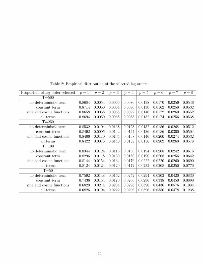
Table 2: Empirical distribution of the selected lag orders.
Proportion of lag order selected p = 1 p = 2 p = 3 p = 4 p = 5 p = 6 p = 7 p = 8T=500
no deterministic term 0.8684 0.0054 0.0066 0.0086 0.0138 0.0170 0.0256 0.0546constant term 0.8714 0.0050 0.0064 0.0090 0.0130 0.0162 0.0258 0.0532
sine and cosine functions 0.8658 0.0058 0.0068 0.0092 0.0140 0.0172 0.0260 0.0552all terms 0.8694 0.0050 0.0068 0.0088 0.0132 0.0174 0.0256 0.0538T=250
no deterministic term 0.8532 0.0104 0.0138 0.0128 0.0132 0.0186 0.0268 0.0512constant term 0.8492 0.0096 0.0142 0.0144 0.0136 0.0186 0.0300 0.0504
sine and cosine functions 0.8466 0.0110 0.0134 0.0138 0.0146 0.0200 0.0274 0.0532all terms 0.8422 0.0076 0.0140 0.0158 0.0156 0.0202 0.0268 0.0578T=100
no deterministic term 0.8344 0.0124 0.0116 0.0156 0.0194 0.0208 0.0242 0.0616constant term 0.8296 0.0118 0.0130 0.0160 0.0190 0.0208 0.0256 0.0642
sine and cosine functions 0.8144 0.0154 0.0134 0.0176 0.0222 0.0220 0.0260 0.0690all terms 0.8124 0.0124 0.0120 0.0172 0.0232 0.0208 0.0250 0.0770
T=50no deterministic term 0.7592 0.0148 0.0162 0.0252 0.0294 0.0302 0.0420 0.0830
constant term 0.7436 0.0154 0.0170 0.0266 0.0296 0.0338 0.0450 0.0890sine and cosine functions 0.6820 0.0214 0.0234 0.0296 0.0390 0.0436 0.0576 0.1034
all terms 0.6826 0.0194 0.0222 0.0296 0.0396 0.0350 0.0478 0.1238
24

Table 3: Empirical Size.tα t1/α F
T=500no deterministic term 0.0518 0.0550 0.0500
constant term 0.0528 0.0542 0.0500sine and cosine functions 0.0514 0.0544 0.0496
all terms 0.0514 0.0532 0.0506T=250
no deterministic term 0.0534 0.0586 0.0584constant term 0.0532 0.0584 0.0558
sine and cosine functions 0.0518 0.0578 0.0572all terms 0.0562 0.0614 0.0576T=100
no deterministic term 0.0632 0.0690 0.0686constant term 0.0640 0.0682 0.0686
sine and cosine functions 0.0594 0.0662 0.0662all terms 0.0674 0.0760 0.0786
T=50no deterministic term 0.0846 0.0940 0.1026
constant term 0.0878 0.0940 0.1104sine and cosine functions 0.0790 0.0860 0.0948
all terms 0.0992 0.1044 0.1230
25

in Section 2 associated to various values of α and test for the capacity to reject the null thatα = 1. The results are given in Figure 1. The results are not size-adjusted. We observe thatthe power properties are relatively satisfactory, increasing with the size sample and somewhatasymmetric.
7 Conclusion
We extend the lag-augmented approach introduced by Toda and Yamamoto (1995), Dolado andLutkepohl (1996) and Yamamoto (1996) to the situation in which seasonal unit roots are presentin the data generating process. This allows the econometrician to test in a VAR frameworkfor linear constraints such as for instance Granger-Causality relationships with non-seasonallyadjusted data. This is of practical interest as we know that separate seasonal adjustmentmay introduce some distortion in the relationships between the variables the economist wantssimultaneously study. The rule we obtain is that if we introduce for a given variable at leastas many additional lags as the number of unit roots present in its individual data generatingprocess, we preserve the fact that the Wald statistic is asymptotically chi-squared distributed.The simulation exercise illustrates that as soon as the sample size is large enough (more than250), size and power properties are satisfactory.
8 References
ANDERSON T.W. [1971], The Statistical Analysis of Time Series, J. Wiley.CANOVA F. and B.E. HANSEN [1995], ‘Are Seasonal Patterns Constant over time? A
Test for Seasonal Stability’, Journal of Business and Economic Statistics, 13, 237-252.CHAN N.H. and C.Z. WEI [1988], ‘Limiting Distribution of Least Squares Estimates of
Unstable Auto regressive Processes’, The Annals of Statistics, 16 (1), 367-401.CUBADDA G. [2001], ‘Complex Reduced Rank models for seasonally cointegrated time
series’, Oxford Bulletin of Economics and Statistics, 63, 497-511.DICKEY D.A. and W. FULLER [1979], ’Distribution of the estimators for autoregres-
sive time series with a unit root’, Journal of the American Statistical Association, 74, 427-431DICKEY D.A., D.P. HASZA and W. FULLER [1984], ‘Testing for Unit Roots in
Seasonal Time Series’, Journal of the American Statistical Association, 79, 355-367.DOLADO J.J and H. LUTKEPOHL [1996], ‘Making Wald tests work for cointegrated
VAR systems’, Econometric Reviews15, 369-386ENGLE R.F , C.W.J. GRANGER and J.HALLMAN [1989], ‘Merging short- and
long-run forecasts: An application of seasonal co-integration to monthly electricity sales fore-casting’, Journal of Econometrics, 40, 45-62.
ENGLE R.F , C.W.J. GRANGER, S.HYLLEBERG and H.S.LEE [1993], ‘Seasonalcointegration: The Japanese consumption function’, Journal of Econometrics, 55, 275-298.
GEWEKE, J. [1979], ‘The Temporal and Sectoral Aggregation of Seasonally AdjustedTime Series’, in Seasonal Analysis of Economic Time Series, Ed. A. Zellner, Washington D.C.,U.S. Bureau of Census, 411-427
GOODMAN N.R. [1963], ‘Statistical analysis based on a multivariate complex Gaussiandistribution (an introduction)’, Annals of Statistics, 34, 152-177.
26

Figure 1: Non adjusted power curves of t and F tests (σ1 = σ2 = 1, ρ = 0.5)
27

GREGOIR S. [1999a], ’Multivariate Time Series with Various Hidden Unit Roots: Part I: Integral Operator Algebra and Representation Theory’, Econometric Theory,15, 435-468.
GREGOIR S. [1999b], ’Multivariate Time Series with Various Hidden Unit Roots: PartII : Estimation and Testing’, Econometric Theory,15, 469-518.
GREGOIR S. [2006], ’Efficient tests for the presence of a pair of complex conjugate unitroots in real time series’, Journal of Econometrics, 130 (1) , 45-100.
GREGOIR S. [2010], ’Fully Modified Estimation of Seasonally cointegrated processes’,Econometric Theory, forthcoming.
HANSEN B.E. [1992], ‘Convergence to Stochastic Integrals for Dependent HeterogeneousProcesses’, Econometric Theory, 8,(4),489-500.
HARRIS D. [1997], ‘Principal components analysis of cointegrated time series’, Econo-metric Theory, 13, 529-557
HYLLEBERG S., R.F.ENGLE, C.W.J.GRANGER and B.S.YOO [1991], ‘SeasonalIntegration and Cointegration’, Journal of Econometrics, 44, 215-238.
JOHANSEN S. [1988], ‘Statistical analysis of cointegration vectors’, Journal of EconomicsDynamics and Control, 12, 231-254
JOHANSEN S. [1991], ‘Estimation and hypothesis testing of cointegration vectors inGaussian vector autoregressive models’, Econometrica, 59, 1551-1580
JOHANSEN S. and E.SCHAUMBURG [1999] ’Likelihood Analysis of Seasonal Coin-tegration’, Journal of Econometrics, 88(2), 301-339
KUROZUMI E. and T.YAMAMOTO [2000], ‘Modified lag augmented vector autore-gressions’, Econometric Reviews, 19, 207-231
LEE J.H. [1992], ‘Maximum likelihood inference on cointegration and seasonal cointegra-tion’, Journal of Econometrics, 54, 1-48
PHILLIPS P.C.B. and P. PERRON [1988], ‘Testing for a unit root in time series re-gression’, Biometrika, 75 (2), 971-1001.
PORTER R.D. [1975] ‘Multiple time series containing unobserved components’, SpecialStudies Paper, n65, Federal Reserve Board
REIMERS H-E [1992] ’Comparisons of tests for multivariate cointegration’, StatisticalPapers, 33, 335-346
RODRIGUES P.M.M. and A.M.R. TAYLOR [2007], ’Efficient test of the seasonalunit root hypothesis’, Journal of Econometrics
SIMS, C.A. [1974], ‘Seasonality in Regression’, Journal of the American Statistical Asso-ciation, 69, 618-626.
SIMS, C.A. , J.H. STOCK and M.W.WATSON [1990], ’Inference in linear time serieswith some unit roots’, Econometrica, 58, 113-144
STOCK J.H and M.W. WATSON [1988], ’Testing for common trends’, Journal of theAmerican Statistical Association, 83, 1097-1107.
TODA H.Y. [1995] ’Finite sample performance of likelihood ratio tests for cointegratingranks in vector autoregressions’, Econometric Theory, 11, 1015-1032
TODA H.Y. and P.C.B. PHILLIPS [1993], ’Vector autoregressions and causality’, Econo-metrica, 61, 1367-1393
TODA H.Y. and T. YAMAMOTO [1995], ’Statistical infrence in vector autoregressionswith possibly integrated processes’, Journal of Econometrics, 66, 225-250
28
TSAY R.S. and G.C. TIAO [1990],‘Asymptotic properties of multivariate nonstationaryprocesses with applications to auto regressions’, Annals of Statistics, 18, 220-250.
WALLIS, K.F. [1974], ‘Seasonal Adjustment and the Relation between Variables’, Journalof the American Statistical Association, 69, 18-32.
WALLIS, K.F. [1976], ‘Seasonal Adjustment and Multiple Time Series Analysis’,in Sea-sonal Analysis of Economic Time Series, Ed. A.Zellner, Washington D.C., U.S. Department ofCommerce, Bureau of Census, 366-397
YAMADA Y. and H.Y.TODA [1998], ’Inference in possibly integrated vector autore-gressive models: some finite sample evidence’, Journal of Econometrics, 86, 55-95
YAMAMOTO T. [1996], ‘A simple approach to the statistical inference in linear timeseries models which may have some unit roots’, Hitotsubashi Journal of Economics, 37, 87-100
9 Appendix
Proof of Theorem 5: The proof is by induction and relies on a polynomial division by ascendingorder. We denote ∆x,j the coefficients of the polynomial ∆x (L)
∆x (L) =dx∑j=0
∆x,jLj
where ∆x,0 = 1. By convention, when the index j is larger than dx, ∆x,j = 0. We set φ(1) (L) =φ (L) and R(1) (L) = 0. The first step consists of computing the first order polynomial remainderdefined by
φ (L)− φ1∆ (L)L =
p∑j=1
φjLj − φ1
dx∑l=0
∆x,lLl+1
=
p∑j=1
(φj − φ1∆x,j−1)Lj −
dx+1∑l=p+1
φ1∆x,l−1Ll
=
p∑j=2
(φj − φ1∆x,j−1)Lj − Lp+1
(dx−p∑l=0
φ1∆x,p+lLl
)where the second term in the right-hand side of the last equation is equal to 0 if dx ≤ p . Letus denote
φ(2) (L) =
p∑j=2
(φj − φ1∆x,j−1)Lj
=
p∑j=2
φ(2)j Lj
a polynomial matrix whose minimal degree is equal to 2 and maximal one to p, and
R(2) (L) = −
(dx−p∑l=0
φ1∆x,p+lLl
)29

a polynomial matrix of degree at most dx − p− 1, we have
φ (L) = φ(1) (L) + Lp+1R(1) (L)
= φ(1)1 ∆ (L)L+ φ(2) (L) + Lp+1R(2) (L)
and (φ
(1)1 φ
(2)2 . . . φ
(2)p
)=(φ
(1)1 φ
(1)2 . . . φ
(1)p
)N (1) ⊗ In
where
N (1)
(p×p)=
1 −∆x,1 −∆x,p−1
0 1 0 0...
. . ....
0 · · · 0 1
We now define (i) a sequence of polynomial matrices
φ(j) (L)
j=2,...,p
whose matrix coefficients
are given by the following recurrence equation
φ(j)k = 0 for 1 ≤ k ≤ j − 1
φ(j)k = φ
(j−1)k − φ
(j−1)j−1 ∆x,k−j+1 for j ≤ k ≤ p
or similarly(φ
(j−1)j−1 φ
(j)j . . . φ
(j)p
)=(φ
(j−1)j−1 φ
(j−1)j . . . φ
(j−1)p
)N (j−1) ⊗ In
where
N (j−1)
(p−j+2×p−j+2)=
1 −∆x,1 −∆x,p−j+1
0 1 0 0...
. . ....
0 · · · 0 1
(ii) a sequence of polynomial matrices
R(j) (L)
j=2,...,p
given by the following recurrence equa-tion
R(j) (L) = R(j−1) (L)−dx+j−p−2∑
k=0
φ(j−1)j−1 ∆x,p−j+kL
k
where the degree of the second term of the right-hand side of the last equation is at mostdx + j − p− 2, which is increasing with j.
We claim that for j = 1, . . . , p
φ (L) =
j−1∑k=1
φ(k)k ∆ (L)Lk + φ(j) (L) + Lp+1R(j) (L)
30

This holds for j = 1 and j = 2. Let assume that it holds up to order j < p− 1. We then have
φ(j) (L)− φ(j)j ∆x (L)Lj =
p∑k=j
φ(j)k Lk − φ
(j)j
dx∑l=0
∆x,lLl+j
=
p∑k=j
(φ
(j)k − φ
(j)j ∆x,k−j
)Lk −
dx+j∑l=p+1
φ(j)j ∆x,l−jL
l
=
p∑k=j
φ(j+1)k Lj − Lp+1
(dx+j−p−1∑
l=0
φ(j)j ∆x,p+l+1−jL
l
)
= φ(j+1) (L) + Lp+1
(−
dx+j−p−1∑l=0
φ(j)j ∆x,p+l+1−jL
l
)
therefore
φ (L) =
j∑k=1
φ(k)k ∆ (L)Lk + φ(j+1) (L)
+Lp+1
(R(j) (L)−
dx+j−p−1∑l=0
φ(j)j ∆x,p+l+1−jL
l
)
=
j∑k=1
φ(k)k ∆ (L)Lk + φ(j+1) (L) + Lp+1R(j+1) (L)
When j = p, since φ(p+1) = 0, we get
φ (L) =
p∑k=1
φ(k)k ∆ (L)Lk + Lp+1
(R(p) (L)−
dx−1∑l=0
φ(p)p ∆x,l+1L
l
)
We set ψ (L) =∑p
k=1 φ(k)k Lk and R (L) = R(p) (L)−
∑dx−1l=0 φ
(p)p ∆x,l+1L
l whose degree is dx− 1.If we denote M (1) = N (1) and for j > 2
M (j) =
(Ij−1 00 N (j−1)
)we set M = M (1)...M (p−1), so that(
φ(1)1 φ
(2)2 . . . φ
(p)p
)=(φ1 φ2 . . . φp
)M ⊗ In
where M is a full rank matrix as a upper triangular matrix with diagonal terms equal to 1.Q.E.D.
Proof of Lemma 7: The proof amounts to show that the set of dx polynomials(∪Sj=1
∆x,−j, δωj
∆x,−j, δ2ωj
∆x,−j, . . . δdj−1ωj
∆x,−j
)31

is a basis of the polynomials of degree less or equal to dx − 1. Indeed, if this is true, anypolynomial q (L) of degree less or equal to dx − 1 can be decomposed in these basis elements,
i.e. there exists a set of numbers
(qjk)k=0,...dj−1
j=1,...S
such that
q (L) =S∑j=1
dj−1∑k=0
qjkδkωj
∆x,−j
=
S∑j=1
dj−1∑k=0
qjkδkωj
∆x,−j
This is true for each coefficient of a polynomial matrix, so it holds for the polynomial matrixitself. To show that the above set of polynomials is a basis we establish it is a set of linearlyindependent elements that generates polynomials of degree less or equal to dx − 1. We start
with the independence property. Let us consider a set of numbers
(qjk)k=0,...dj−1
j=1,...S
such
that q (L) = 0. We partition the set 1, ..., S into subsets of index related to frequencies thathave the same order of integration:
1, ..., S =
maxj dj⋃k=1
Jk
withJk = j ∈ 1, ..., S |dj = k
and
q (L) =
maxj dj∑k=1
∑j∈Jk
(k−1∑l=0
qjlδlωj
)∆x,−j
We denote Kj = ∪jk=1Jk. We proceed by induction on k. First, we compute the value of q (L)at each unit root and get ∀j ∈ 1, . . . , S
q(eiωj)
= qj0∆x,−j(eiωj)
= 0
=⇒ qj0 = 0
since ∀k 6= j, ∆x,−k (eiωj) = 0, then
q (L) =
maxj dj∑k=2
∑j∈Jk
(k−1∑l=1
qjlδl−1ωj
)δωj
∆x,−j
If we compute the derivative of this polynomial, we get
q′ (L) =
maxj dj∑k=2
∑j∈Jk
(k−1∑l=2
(l − 1) qjlδl−2ωj
)δωj
∆x,−j+
maxj dj∑k=2
∑j∈Jk
(k−1∑l=1
qjlδl−1ωj
)[δωj
∆′x,−j − eiωj∆x,−j
]
32

which is equal to zero. We compute the value of q′ (L) at each unit root whose index is in J\K2
we get that ∀j ∈ J\K2
q′(eiωj)
= −qj1eiωj∆x,−j(eiωj)
= 0
=⇒ qj1 = 0
and then
q (L) =
maxj dj∑k=3
∑j∈Jk
(k−1∑l=2
qjlδl−2ωj
)δ2ωj
∆x,−j
+∑j∈J2
qj1δωj∆x,−j
This result holds because the value of the derivative of ∆x,−k at eiωj when j is in J\K2 is zerodue to fact that the monomial associated to this unit root is raised at a power strictly largerthan 1 in ∆x,−k. Let us assume that when we repeat this kind of operations h times, we getthe following form for q (L) :
q (L) =
maxj dj∑k=h+1
∑j∈Jk
(k−1∑l=h
qjlδl−hωj
)δhωj
∆x,−j (18)
+h∑k=2
∑j∈Jk
qj,k−1δk−1ωj
∆x,−j
We compute the derivative of order h. We take in turn each polynomial in this sum and start bythose in the second term. We use the property that when j ∈ J\Kh, the value of the derivativeof order h of ∆x,−k at eiωj for any k 6= j is zero due to fact that the monomial associated tothis unit root is raised at a power strictly larger than h in ∆x,−k. By Leibnitz rule, we get thatfor j ∈ Kh,
dh
dLh
(qj,k−1δ
k−1ωj
∆x,−j
)= qj,k−1
h∑l=0
(h
l
)dl
dLlδk−1ωj
dh−l
dLh−l∆x,−j
and conclude that its value at each unit root whose index is in J\Kh is 0 by the above property.For j ∈ J\Kh, we get
dh
dLh
dj−1∑g=h
qjgδg−hωj
δhωj∆x,−j
=h∑l=0
(h
l
)dl
dLl
dj−1∑
g=h
qjgδg−hωj
δhωj
dh−l
dLh−l∆x,−j
When we compute the value of the term at a unit root whose index j′ ∈ J\Kh, by the aboveproperty, the only non zero term is the one when l = h and j′ = j. This implies that forj ∈ J\Kh
dhq (eiωj)
dLh= h! (−1)h eihωj∆x,−j
(eiωj)
= 0
=⇒ qjh = 0
33

This ensures that (18) holds at the order h+ 1. By induction, we conclude that
q (L) =
maxj dj∑k=2
∑j∈Jk
qj,k−1δk−1ωj
∆x,−j
or
q (L) =
maxj dj∑k=1
∑j∈Jk
qj,k−1
∏l 6=j
δωl
∆x
S∏j=1
δωj
= 0
In this product, the second polynomial is different from 0, the first one is therefore exactlyequal to 0. If we compute its value in each unit root ωj we conclude that qj,dj−1 = 0 . Thisfamily is linearly independent. The dimension of the vector space of polynomials of degree lessthat dx − 1 is exactly equal to dx . The above family is composed of dx linearly independentelements, it is therefore a basis of the space of polynomials of degree less that dx − 1.
Q.E.D.Proof of Lemma 9: We start from the equivalent representations of the generating equationwith additional lags written with matrix notations in equations (4.3,13)
y = βτ + φy−1 + Φy−pa + ε
y = βτ + ψ∆xy + ξ∆xy−p +Rz−p + ε
y = βτ + ψ∆xy + Rz−p + ε
where according Theorem 5, Lemma 7 and the attached comment we know there exist twomatrices M and K of respective dimensions (pa − dx − 1× pa − dx − 1) and (p× dx − 1) suchthat (
φ Φ)(M ⊗ In) =
(ψ ξ
)(φ Φ
)(K ⊗ In) = R
and M is upper triangular so that there exists with obvious notations a (p× p) matrix M11
such thatφ (M11 ⊗ In) = ψ
orvecψ = [(M ′
11 ⊗ In)⊗ In] vecφ
The test statistics have the following form
ζW = f(vecφ
)′ [ ∂f
∂vecφ′
((y−1Py−pa
y′−1
)−1 ⊗ Ωε
) ∂f ′
∂vecφ
]−1
f(vecφ
)and
ζ ′W = g(vecψ
)′ [ ∂g
∂vecψ′
((∆xyPz−p∆xy
′)−1
⊗ Ωε
)∂g′
∂vecψ
]−1
g(vecψ
).
On the one hand,∂g
∂vecψ′=
∂f
∂vecφ′[(M−1
11 ⊗ In)⊗ In
]34
on the other hand, with obvious notations
φy−1 + Φy−pa = ψ∆xy + ξ∆xy−p +Rz−p
=(φ Φ
)(M ⊗ In)
(∆xy
∆xy−p
)+(φ Φ
)(K ⊗ In) z−p
= φ (M11 ⊗ In) ∆xy +(
(φ (M12 ⊗ In) + Φ (M22 ⊗ In))(φ Φ
)(K ⊗ In)
)( ∆xy−pz−p
)= φ (M11 ⊗ In) ∆xy +
((φ (M12 ⊗ In) + Φ (M22 ⊗ In))
(φ Φ
)(K ⊗ In)
)z−p
and since each component at date t of z−p is a linear combination of yt−p−1, .. yt−pa , there existsa (dx − 1 + pa − p)× (pa − p) matrix H such that
Hy−pa = z−p,
it follows thatφy−1Py−pa
= φ (M11 ⊗ In) ∆xyPz−p
This holds for any value of φ where y−1Py−pay′−1 and ∆xyPz−p∆xy
′are symmetric definite
positive matrices whence the result.Q.E.D.
Proof of Lemma 15: It is direct application of the joint weak convergences summarized in theLemmata of section 5 and the algebraic results.
35