TESTING FOR GRANGER NON-CAUSALITY

IN COINTEGRATED SYSTEMS

MADE EASY

Alicia N. Rarnbaldi and Howard E. Doran

No. 88- August 1996

ISSN 0 157 0188

ISBN 1 86389 352 0

Testing for Granger Non-Causality in Cointegrated Systems Made Easy.

Alicia N. Rambaldi and Howard E. DoranI

Department of Econometrics

University of New England

Armidale, NSW 2351. Australia

Abstract:

Considerable research has been devoted during the last five years to develop appropriate testsfor Granger-Causality in integrated and cointegrated systems. Despite the existence of severaltests, applied reasearch appears still to be conducted using some form of an F-test in thecontext of a VAR or an ECM. Reasons could be that the appropriate tests have only recentlyappeared in the literature, or that their implementation is relatively complex. This paper showshow to use readily available routines in RATS, SAS and SHAZAM to obtain the WALD testfor Granger non-causality introduced by Toda and Yamamoto (1995).

JEL Classification: C12, C32.

The authors wish to thank Professor tLC.I-rall for valuable help with the SAS routine and ProfessorW.E. Griffiths for useful comments on an earlier version.

2

Testing for Granger Non-causality in Cointegrated Systems Made Easy.

1. Introduction

Testing for Granger non-causality in the context of stable VAR models involves testing

whether some parameters of the model are jointly zero. In the past such testing has involved a

standard F-test in a regression context.

However, recent research (see Toda and Phillips, 1993) has shown that when the

variables are integrated, the F-test procedure is not valid, as the test statistic does not have a

standard distribution.

Many years ago Pierce (1977) discussed the problem of ignoring the effect of

autocorrelation. He concluded that "relatiionships will frequently tend to be ’found’ that don’t

exist ..." A similar problem occurs in this context. If inappropriate tests are used, the

probability of Type I errors may well be (much) larger than the nominal size of the test. Hence,

causal relationships which do not exist may be "discovered".

Toda and Phillips’ result has given rise to the development of several alternative

procedures. First, in cointegrated systems, an Error Correction model (ECM) can be

transformed to its levels VAR form allowing a Wald type test (WALD) for linear restrictions to

the resulting VAR model (WALD), see Ltitkepohl and Reimers (1992) and Toda and Phillips

(1993). Second, Mosconi and Giannini (1992) suggested a likelihood ratio test (LR) for

systems that are cointegrated. Unfortunately, the virtues of simplicity and ease of application

have been largely lost.

3

A third procedure (MWALD) (see Toda and Yamamoto (!995) and Dolado and

Ltitkepohl (1996)) is theoretically very simple, as it involves estimation of a VAR model

augmented in a straightforward way (MWALD). A Monte Carlo experiment which included

these three alternative test procedures, presented in Zapata and Rambaldi (1997), provides

evidence that the MWALD test has comparable performance in size and power to the LR and

WALl3 tests in samples of 50 or more observations. However, as presented in the literature,

the implementation of the test is not entirely straightforward and involves some programming.

Despite the existence of these tests, applied research appears still to be conducted using

some form of an F-test in the context of a VAR or an Error Correction Model (see for

instance: Riezman, Whitman and Summers (1996), Hewarathna and Silvapulle (1996), Shan

and Sun (1996), Erenburg and Wohar (1995), Mizala and Romaguera (1995), Saunders

(1995), and Thorton (1995)). The failure to reach applied economists could be due to the fact

that these tests have only recently appeared in the literature or to the relative complexity of

implementation. Whatever the reason, the purpose of this paper is to show how the theoretical

simplicity of MWALD can be matched by easy computation using the standard facilities of

common computer packages, without the need for programming. Thus, the virtue of the

practical simplicity of the F-test can be re-captured when the variables are integrated or

cointegrated.

The presentation is as follows: Section two sets out the notation and presents the

MWALD test. Section three proves that the quadratic form required to compute the MWALD

test is numerically identical to the chi-squared test obtained by estimating the model as a set of

Seemingly Unrelated Regressions. Section four shows how to use the SUR routines in

SHAZAM, SAS and RATS

summary.

to obtain the MWALD test. Section five provides

4

a brief

2. The MWALD test for non-causality

Toda and Yamamoto (1995) proved that in integrated and cointegrated systems the

Wald test for linear restrictions on the parameters of a VAR(k) has an asymptotic ~2

distribution when a VAR(k + cl~x) is estimated, where d,~ is the maximum order of

integration in the system.

In order to clarify the principle, let us consider the simple example of a bivariate (p=2)

model with one lag (k=l). That is,

xt = At + Alx~.l +et,

or more fully,

LX=,J LC~;oJ Lo~’? °~’~JLx=,,-,, Le~’j

w~e ~ =[e,, ~= 0 ~ ~’~ = ~.J

To test ~t x~ does not Gr~ger cau~ x~, we w~ test the p~eter res~c~on ~) = 0.

now we ~ume ~at x~t ~d x~t ~e I(1), a s~d~d t-test ~ not v~d. Fo~ow~g Dohdo ~d

L~epo~ (1996), we test~,~-(*~ = 0 by com~ct~g ~e usu~ W~d test b~d on ~t ~u~es

es~tes ~ the augmented model:

We will now set down the MWALD test procedure for a general VAR(k) model.

Then,

Let x~ be a vector of p economic variables, x~t .....x~, satisfying a VAR(k) process.

x~ = Ao + &xt.1 +... + Atx~.~ + e~, t=k+l .....T (1)

where ek+l .....eT are ~ iid (0, Z).

Deflrlirlg A = [ Ao A1 ... At] equation (1) can be written in the form:

xt = A xlt + e,t, t - k+l .....T (2)

where,

xl, = [1 x,’_,.., x,’_~]’ (3)

Finally, concatenating observations horizontally by defining

x = [x~+~ x~+2.., xv]

xl= [xlk÷, xlk+2 ... Xlv]

e = [ek+~ ek+2 ... e-r]

equation (2) can be written as

x=Axl +e (4)

The estimate .~ and the variance-covariance, £~,, can be obtained using multivariate least

squares. The estimator of Av, where Av = vec(A), is (see Liitkepohl, 1991):

~.~ = ((xl xl’)"~ ® I~) vec(x)

^

and the estimated variance-covariance of Av is given by

where,

F = (xlxl’)/T*

(5)

6

~ = xMx’/T*

M = IT, - xl’(x! xl’)-1 X!

and,

T*=T-k.

To compute the MWALD test we proceed as follows:

(a) Estimate a VAR(k+c~) process by multivariate least squares2,

(b)

(c)

Then, under the null of non-causality

has an asymptotic Z~j) distribution.

(6)

(7)

where d~,~ is the

maximum degree of integration in the system, to obtain ,~ v, the least squares estimate of

A,.

Estimate Z^ using (5).

Let R be a J × (pk +1) matrix which selects the appropriate ’non-causality’ parameters.

(8)

In the bivariate example presented above, to test that x2 does not Granger cause xl, we

must test:

Ho: -~’- 0

Ho: RAy =0,

or

where R is given by

R=[O000100000]

A likelihood ratio test to empirically determine the value of ’k’ is detailed in Enders (1995) pages 312-315.

~(1) O~ll) ~(1) _(1) ~(2) _(2) _(2) ~(2) "] ¯Av-" Olo 020 ~11 ~12 ~22 ~ll ~21 ~12 ~22 J

7

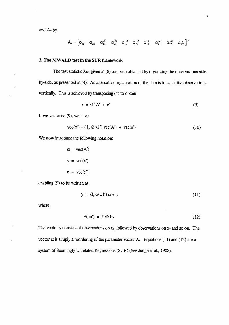
3. The MWALD test in the SUR framework

The test statistic ~.w, given in (8) has been obtained by organising the observations side-

by-side, as presented in (4). An alternative organisation of the data is to stack the observations

vertically. This is achieved by transposing (4) to obtain

x’=xl’A’ + e" (9)

If we vectorise (9), we have

vec(x’) = ( I~, ® xl’) vec(A’) + vec(e’) (10)

We now introduce the following notation:

ot = vec(A’)

y = vec(x¯)

u = vec(e’)

enabling (9) to be written as

y = (Ip®xl’)a+u (11)

where,

E(uu’) = E ® IT, (12)

The vector y consists of observations on xl, followed by observations on x2 and so on. The

vector e~ is simply a reordering of the parameter vector Av. Equations (11) and (12) are a

system of Seemingly Unrelated Regressions (SUR) (See Judge et aL, 1988).

I0

EQUATION YEQ Y# CONSTANT Y{1

EQUATION ZEQ Z# CONSTANT Y{1 9. 3 4 5) Z{1 9. 3 4 5) W{1 9. 3 4 5)

EQUATION WEQ W# CONSTANT Y(1

SUR3# YEQ# ZEQ# WEQTEST (PRINT)#78910#oo o o

~.2. SAS

Assuming the lagged values of y, z and w have been created previously (see Appendix A.2.2for details) the code is:

PROC SYSLIN SUR VARDEF=N;TITLE "WALD TEST USING THE SUR PROCEDURE";Y:MODEL Y = I~LAGI ZLAGI WLAGI YLAG2 ZLAG2 WLAG2 YLAG3 ZLAG3 WLAG3

YLAG4 ZLAG4 WLAG4 YLAG5 ZLAG5 WLAG5;Z :MODEL Z = YLAGI ZLAGI WLAGI YLAGg. ZLAGg. WLAG2 YLAG3 ZLAG3 WLAG3

YLAG4 ZLAG4 WLAG4 YLAG5 ZLAG5 WLAG5;W:MODEL W = YLAGI ZLAGI WLAGI YLAGg. ZLAGg. WLAGg. YLAG3 ZLAG3 WLAG3

YLAG4 ZLAG4 WLAG4 YLAG5 ZLAG5 WLAG5;STEST Y.ZLAGI--0, Y.ZLAGg.=0, Y.ZLAG3=0, Y.ZLAG4=0;RUN;

Note that in SAS the value ofL~, = J × ’numerator’, that is the value labelled ’numerator’multiplied by the number of restrictions (J).

4.3 SHAZAM

Assuming the lagged values of y, z and w have been created previously (see Appendix A.2.3for details) the code is:

sample 6 I00system 3 / dnols y ly Iz lw 12y 12z 12w 13y 13z 13w 14y 14z 14w 15y 15z 15wols z ly Iz lw 12y 12z 19.w 13y 13z 13w 14y l~z 14w 15y 15z 15wols w ly Iz lw 19.y 12z 19.w 13y 13z 13w 14y 14z 14w 15y 15z 15wtesttest iz:l=0

test 12z:l--Otest 13z:l=Otest 14z:l=Oend

11

5. Sulranary

This paper has presented a method for the practical implementation of the Toda and

Yamamoto (1995) Wald test for Ganger non-causality in integrated and cointegrated systems.

We have shown that the numerical value of the required Wald test can be obta~ed by using the

Seemingly Unrelated Regressions routine readily available in econometrics packages. The

codes for RATS, SAS and SHAZAM have been included for the reader’s future reference.

12

6. References

Dolado, J. J. and H. Lt~tkepohl (!996). Making Wald Tests Work for Cointegrated VARSystems. Econometric Reviews, forthcoming.

Enders, W. (1995). Applied Econometric Time Series. (¥v’iley, New York).

Erenburg, S. and M. Wohar (1995). Public and Private Investment: Are there causal linkages?,Journal ofMacroeconomics, Vol. 17, 1-30.

Hewarathna, R. and P. Silvapulle (1996). An Empirical Investigation of the RelationshipsAmong Real, Monetary and Financial Variables: Australian Evidence, in M. McAller, P. Millerand K. Leong Proceddings of the Econometric Society Australasian Meeting, Vol 3, 493-516.

Judge,G. G., R.C. Hill, W.E. Griffiths, H. Ltitkepohl, and T. Lee (1988). The Introduction tothe Theory and Practice of Econometrics, 2nd Edition. (Wiley, New York).

Ltitkepohl, H. (1991). Introduction to Mul~ple Time Series (Springer-Verlag, Berlin).

Ltitkepohl, H. and H. Reimers (1992). Granger-Causality In Cointegrated VAR Processes,Economic Letters, Vol. 40, 263-268.

Mizala, A. and P. Romaguera (1995). Testing for Wage Leadership Processes in the ChileanEconomy, Applied Economics, Vok 27, 303-310.

Mosconi, R and C. Giannini (1992). Non-Causality in Cointegrated Systems: Representation,Estimation and Testing, Oxford Bulletin of Economics and Statistics, Vok 54 No. 3,399-417.

Pierce, D. (1977). Relationships-and the Lack Thereof-Between Economic Time Series, withSpecial Reference to Money and Interest Rates, Journal of the American StatisticalAssociation, Vol. 72, 11-22.

Riezman, R. C. Whiteman and P. Summers (1996). The Engine of Growth or its handmaiden?A Time-Series Assessment of Export-Led Growth, Empirical Economics, Vol. 21, 77-110.

Saunders, P. A Granger Causality Approach to Investigating the impact of Fiscal Policy on theU.S. Economy, Studies in Economics and Finance, Vol. 16, 3-22.

Shan, J. and R. Sun (1996). A Granger-Sims Causality Test for Domestic Savings and ForeignCapital in Indonesia, in McAller, Miller and Leong Proceddings of the Econometric SocietyAustralasian Meeting, Vol 3, 301-320.

Toda, H. Y. and P. C. B. Phillips (1993).Econometrica, Vol. 61 No.6, 1367-1393.

Vector Autoregressions and Causality,

!3

Toda, H. Y. and T. Yamamoto (!995). Statistical Inference in Vector Autoregressions withPossibly Integrated Processes, Journal of Econometrics, Vol. 66, 225-250.

Thorton, J. (1995). Friedman’s Money Supply Volatility Hypothesis: Some IntemationalEvidence, Journal of Money, Credit and Banking, Vol. 27, 288-292.

Zapata, H.O. and A. N. Rambaldi (1997). Monte Carlo Evidence on Cointegration andCausation, Oxford Bulletin of Economics and Statistics, Vol. 59, forthcoming.

14

Appendix

A.1 Computing MWALD using matrix manipulation

(1) Program

/* COMPUTING THE WALD TEST OF TODA AND YAMAMOTO(1995) AND* DOLADO AND LUTKEPOHL (1996).* THIS PROGRAM HAS BEEN WRITTEN IN GAUSS.* LINES BETWEEN "~**~****" AND MARKED "<<<<<" NEED TO BE CHANGED* ACCORDING TO DATA SET

loaddat[100,3] = example.dat;

y = dat[.,l];z = dat[.,2];w = dat[.,3];p = 3;k = 5;t = rows(dat) - k;

x = dat[k+l:rows(dat),l:p]’; /* VECTOR OF DEPENDENT VARIABLES */

ly = zeros(rows(dat),k);iz = zeros(rows(dat),k);lw = zeros(rows(da~),k);

i = I;do while i <= k;

ly[.,i] = lagn(y,i);Iz[.,i] = lagn(z,i);lw[.,i] = lagn(w,i);

i = i + I;endo;

xl = zeros(k*p+l,t);x111,.] = ones(1,t);

i = 1; j = 4;do while i <= k;

xl[i+j:i*p+l,.] = (ly[k+l:rows(dat),i])’ I(iz [k+l :rows (dat), i] ) ’ I(lw[k+l : rows (dat) ,i] ) ’ ;

j --j +~.;i = i + i;

endo;

output file =mwald.out reset;

-++++++++++++WALD TEST IN AUGMENTED VAR +++++++++++++++++++++++";

vahat = ((inv(xl*xl’)*xl) .*. eye(p))*vec(x);

15

(1/T)*(xl*xl’);eye(T);(I/T)* x*(i-xl’*inv(xl*xl’)*xl)*x’;

siwa = inv(g) .* O;

r = zeros(4,48);r[l,7] = 1;r[2,16] = 1;r[3,25] = 1;r[4,34] = I;

/* <<<<<<<<< CHANGE ACCORDINGLY *//* <<<<<<<<< CHANGE ACCORDINGLY *//* <<<<~<<<< CHANGE ACCORDINGLY *//* <<<<<<<<< CHANGE ACCORDINGLY *//* <<<<~<<<< CHANGE ACCORDINGLY */

1 = t*(r*vahat)’*inv(r*siga*r’)*(r*vahat);

VAR ( k+ 1 ) OUTPUT

FORMAT /RD /MI 12,6;"Vector Ahat = " vahat;

"Value of MWALD = " i;

output off;end;

(2) Output

++++++++++++WALD TEST IN AUGMENTED VAR +++++++++++++++++++++++VAR(k+I) OUTPUT

Vector Ahat =-0.135319

0.089166-0.094066

0.6104870.0370540.054125

-0.1081721.1515030.2979940.094815

-0.2625640.553337

-0.119507-0.332908-0.335877-0.436204-0 297336-0 424655

0 4032910 5088310 6481320 1349110 4845710 6673780 0903420 0299460.081160

-0.064501-0.325685-0.461509-0.073140

0.1504210.0919130.122368

16

0.1345180.3090890.120483

-0.0915620.014071

-0.108224-0.326706-0.393981-0.258383-0.088364-0.299372-0.006420

0.2078150.193092

Value of MWALD = 16.965899

A.2 Computing MWALD using the SUR routine

A.2.1 RATS

(1)Program

CAL 1960 1 4ALL i0 1990:4OPEN DATA EXAMPLE.DATDATA(FORMAT=FREE,ORG=OBS)/ YZW

EQUATION YEQ Y# CONSTANT Y{1 2 3 4 5) Z{I 2 3 4 5) W{1 2 3 4 5}

EQUATION ZEQ Z# CONSTANT Y{1 2 3 4 5} Z{1 2 3 4 5} W{1 2 3 4 5}

EQUATION WEQ W# CONSTANT Y{1 2 3 4 5} Z{1 2 3 4 5} W{1 2 3 4

SUR3# YEQ# ZEQ# WEQTEST (PRINT)#78910#ooo o

(2) Output

Dependent Variable Y - Estimation by Seemingly Unrelated RegressionsQuarterly Data From 1961:02 To 1984:04Usable Observations 95Centered R**2 0.961389Uncentered R**2 0.996655Mean of Dependent VariableStd Error of Dependent VariableStandard Error of EstimateSum of Squared ResidualsDurbin-Watson Statistic

Degrees of FreedomR Bar **2 0,954057T x R**2 94.682-4.393564211

1.3603195780.291574095

6.71622079972.018157

79

]7

Variable Coeff Std Error T-Star Signif

123456789i0.II.12.13.14.15.16.

Constant -0.135318861 0.099151193 -1.36477Y{I) 0.610487113 0.163603508 3.73150Y{2} -0.119506609 0.190519196 -0.62727Y{3] 0.134910599 0.190327421 0.70883Y{4} -0.073139742 0.191866565 -0.38120Y{5} -0.108223530 0.150044267 -0.72128Z{I} -0.108172314 0.136079742 -0.79492Z{2} -0.436204028 0.176785837 -2.46742Z{3} 0.090341596 0.185539494 0.48691Z{4) 0.122367785 0.181941134 0.67257Z{5) -0.258382550 0.147597829 -1.75059W{I) 0.094814777 0.153354242 0.61827W{2) 0.403291237 0.182999217 2.20379W{3} -0.064500931 0.189318103 -0.34070W{4] 0.120482716 0.190972147 0.63089W{5} -0.006420483 0.149921769 -0.04283

Dependent Variable Z - Estimation by Seemingly Unrelated RegressionsQuarterly Data From 1961:02 To 1984:04Usable Observations 95Centered R**2 0.963283Uncentered R**2 0.986081Mean of Dependent VariableStd Error of Dependent VariableStandard Error of EstimateSum of Squared ResidualsDurbin-Watson Statistic

Degrees of FreedomR Bar **2 0.956312T x R**2 93.678-2.2553101471.7715357870.370282518

10.8316223122.109382

79

0.172324440.000190340.530483530.478427330.703054050 470738900 426660870 013609250 626319970 501222160 080017420 536395440 027539350 733328430 528111430 96584059

Variable Coeff Std Error T-Star Signif

17. Constant 0.089165972 0,125916376 0.70814 0.4788605418. Y{I} 0.037054231 0.207767150 0.17834 0.8584520419. Y{2} -0.332908069 0.241948543 -1.37595 0.1688384320. Y{3} 0.484570553 0.241705000 2.00480 0.0449842721. Y{4} 0.150420975 0.243659625 0.61734 0.5370101122. Y{5} -0.326706177 0.190547685 -1.71456 0.0864252223. Z{I} 1.151502959 0.172813533 6.66327 0.0000000024. Z{2} -0.297335968 0.224507959 -1.32439 0.1853737425. Z{3} 0.029945732 0.235624605 0.12709 0.8988684926. Z{4} 0.134517663 0.231054893 0.58219 0.5604392527. Z{5] -0.088363661 0.187440849 -0.47142 0.6373397128. w{l] -0.262563512 0.194751166 -1.34820 0.1775940829. W{2} 0.508830552 0.232398597 2.18947 0.0285624530. W{3} -0.325684940 0.240423223 -1.35463 0.1755349031. W{4} -0.091561603 0.242523766 -0.37754 0.7057748532. W{5} 0.207815140 0.190392120 1.09151 0.27504799

Dependent Variable W - Estimation by Seemingly Unrelated RegressionsQuarterly Data From 1961:02 To 1984:04Usable Observations 95Centered R**2 0.973440Uncentered R**2 0.997283Mean of Dependent VariableStd Error of Dependent variableStandard Error of EstimateSum of Squared ResidualsDurbin-Watson Statistic

Degrees of FreedomR Bar **2 0.968397T x R**2 94.742-6.592059684

2.2369878350.397677328

12.4936333012.042989

79

Variable Coeff Std Error T-Star Signif

33. Constant -0.094066184 0.135232115 -0.69559 0.4866852734. Y{I] 0.054124983 0.223138498 0.24256 0.8083445135. Y{2} -0.335877144 0.259848752 -1.29259 0.1961539036. Y{3} 0.667378178 0.259587191 2.57092 0.0101428437. Y{4} 0.091913042 0.261686426 0.35123 0.7254131738. Y{5) -0.393981198 0.204645077 -1.92519 0.0542052639. Z[I} 0.297993701 0.185598889 1.60558 0.1083664240. Z{2} -0.424655472 0.241117851 -1.76119 0.0782054641. Z{3) 0.081159600 0.253056946 0.32072 0.7484250642. Z{4} 0.309088925 0.248149150 1.24558 0.2129196643. Z{5] -0.299372161 0.201308385 -1.48713 0.1369799344. W{I} 0.553336982 0.209159545 2.64553 0.00815641

2O

Model: WDependent variable: w

WALD TEST USING THE SUR PROCEDURE

SYSLIN ProcedureSeemingly Unrelated Regression Estimation

Parameter EstimaSes

Parameter Standard T for H0:Variable DF Estimate Error Parameter=0

INTERCEPYLAGIZLAGIWLAGIYLAG2ZLAG2WLAG2YLAG 3ZLAG3WLAG3YLAG4ZLAG4WLAG4YLAG5ZLAG5WLAG5

1111111111111111

-0 0940660 0541250 2979940 553337

-0 335877-0 4246550 6481320.6673780.081160

-0.4615090.0919130.3090890.014071

-0.393981-0.2993720.193092

Prob > IT1

0.135232 -0.696 0.48870.223138 0.243 0.80900.185599 1.606 0.11240.209160 2.646 0.00980.259849 -1.293 0.19990.241118 -1.761 0.08210.249592 2.597 0.01120.259587 2.571 0.01200.253057 0.321 0.74930.258211 -1.787 0.07770.261686 0.351 0.72630.248149 1.246 0.21660.260467 0.054 0.95710.204645 -1.925 0.05780.201308 -1.487 0.14100.204478 0.944 0.3479

Test:Numerator: 4. 241475 DF: 4 F Value: 3.5271

Denominator: 1.202532 DF: 237 Prob>F: 0.0081

Then, ~w = 4 × 4.241475 = 16.965899

A.2.3 SHAZAM

(1) Program:

read(example.dat) ygenr ly = lag(y)genr 12y = lag(y,2)gent 13y = lag(y,3)gear 14y = lag(y,4)genr 15y = lag(y, 5)gemr iz = lag(z)genr 12z = lag(z,2)genr 13z = lag(z,3)gent 14z = lag(z,4)gear 15z = lag(z,5)gent lw = lag(w)genr 12w = lag(w,2)gent 13w = lag(w, 3)genr 14w = lag(w,4)gear 15w = lag(w,5)

sample 6 I00

z w

21

system 3 / dnols y ly iz lw 12y 12z 12w !3y 13Z 13w 14y 14z 14w 15y 15Z 15wols Z ly iz IW 12y 12Z l~w 13y 13z 13w 14y 14Z 14w 15y 15z 15wOIs w ly IZ IW 12y 12Z 12w 13y 13Z !3w 14y 14Z 14w 15y 15z 15wtest

test iz:l=Otest 12z:l=Otest 13z:l=Otest 14z:l=Oendstop

(2) Relevant Output:

EQUATION 1 OF 3 EQUATIONSDEPENDENT VARIABLE = Y 95 OBSERVATIONS

R-SQUARE = .9614VARIANCE OF THE ESTIMATE-SIGMA**2 = .70697E-01STANDARD ERROR OF THE ESTIMATE-SIGMA = .26589SUM OF SQUARED ERRORS-SSE= 6.7162MEAN OF DEPENDENT VARIABLE = -4.3936LOG OF THE LIKELIHOOD FUNCTION = -11.1823

ASYMPTOTICVARIABLE ESTIMATED STANDARD T-RATIO

NAME COEFFICIENT ERRORLY .61049 .1636 3.732LZ -.10817 .1361 -.7949LW .94815E-01 .1534 .6183L2Y -.11951 .1905 -.6273L2Z -.43620 .1768 -2.467L2W .40329 .1830 2.204L3Y .13491 .1903 .7088L3Z .90342E-01 .1855 .4869L3W -.64501E-01 .1893 -.3407L4Y -.73140E-01 .1919 -.3812L4Z .12237 .1819 .6726L4W .12048 .1910 .6309L5Y -.10822 .1500 -.7213LSZ -.25838 .1476L5W -.64205E-02 .1499CONSTANT -.13532 .9915E-01

PARTIAL STANDARDIZED ELASTICITYP-VALUE CORR. COEFFICIENT AT MEANS

00042753653O014O28478626733703501528471

-1.751 080-.4283E-01 966-1.365 172

.387-.089

.069-.070- .267

.241

.079

.O55-.038-.043

.075

.071-.081-.193-.005-.152

.6026-.1416

.1593-.1172-.5729

.6896

.1314

.118711230709159921311056333701160000

611705451414119921515979135504360950

- 073505771763

-.1087-.1189-.0093

.0308

EQUATION 2 OF 3 EQUATIONSDEPENDENTVARIABLE = Z 95 OBSERVATIONS

R-SQUARE = .9633VARIANCE OF THE ESTIMATE-SIGMA**2 = .11402STANDARD ERROR OF THE ESTIMATE-SIGMA : .33766SUM OF SQUARED ERRORS-SSE: 10.832MEAN OF DEPENDENT VARIABLE = -2.2553LOG OF THE LIKELIHOOD FUNCTION : -11.1823

ASYMPTOTICVARIABLE ESTIMATED STANDARD T-RATIO

NAME COEFFICIENT ERRORLY .37054E-01 .2078 .1783LZ 1.1515 .1728 6.663

PARTIAL STANDARDIZED ELASTICITYP-VALUE CORR. COEFFICIENT AT MEANS

.858 .020 .0281 .0723

.000 .600 1.1574 1.1295

24

An Error Components Model for Prediction of County Crop Areas Using Survey andSatellite Data. George E. Battese and Wayne A. Fuller, No. 15 - February !982.

Networking or Transhipment? Optimisation Alternatives for Plant Location Decisions.H.I. Tof~ and P.A. Cassidy, No. 16 - February 1985.

Diagnostic Tests for the Partial Adjustment and Adaptive Expectations Models.H.E. Doran, No. 17 - February 1985.

A Further Consideration of Causal Relationships Between Wages and Prices.J.W.B. Guise and P.A.A. Beesley, No. 18 - February 1985.

A Monte Carlo Evaluation of the Power of Some Tests For Heteroscedasticity.W.E. Griffiths and K. Surekha, No. 19 - August 1985.

A Walrasian Exchange Equilibrium Interpretation of the Geary-Khamis InternationalPrices. D.S. Prasada Rao, No. 20 - October 1985.

On Using Durbin’s h-Test to Validate the Partial-Adjustment Model. H.E. Dorart, No. 21 -November 1985.

An Investigation into the Small Sample Properties of Covariance Matrix and Pre-TestEstimators for the Probit Model. William E. Griffiths, R. Carter Hill and Peter J.Pope, No. 22 - November 1985.

A Bayesian Framework for Optimal Input Allocation with an Uncertain StochasticProduction Function. William E. Gfiffiths, No. 23 -February 1986.

A Frontier Production Function for Panel Data: With Application to the Australian DairyIndustry. T.J. Coelli and G.E. Battese, No. 24 - February 1986.

Identification and Estimation of Elasticities of Substitution for Firm-Level ProductionFunctions Using Aggregative Data. George E. Battese and Sohail J. Malik, No. 25 -April 1986.

Estimation of Elasticities of Substitution for CES Production Functions Using AggregativeData on Selected Manufacturing Industries in PaMstan. George E. Battese andSohail J. Malik, No. 26 - April 1986.

Estimation of Elasticities of Substitution for CES and VES Production Functions UsingFirm-Level Data for Food-Processing Industries in Pakistan. George E. Battese andSohail J. Malik, No. 27 - May 1986.

On the Prediction of Technical Efficiencies, Given the Specifications of a GeneralizedFrontier Production Function and Panel Data on Sample Firms. George E. Battese,No. 28 - June 1986.

25

A General Equilibrium Approach to the Construction of Multilateral Index Numbers.D.S. Prasada Rao and J. Salazar-Carrillo, No. 29 - August 1986.

Further Results on Interval Estimation in an AR(1) Error Model. H.E. Doran,W.E. Griffiths and P.A. Beesley, No. 30 - August 1987.

Bayesian Econometrics and How to Get Rid of Those Wrong Signs. W’flliarn E. Griffiths,No. 31 - November 1987.

Confidence Intervals for the Expected Average Marginal Products of Cobb-DouglasFactors With Applications of Estimating Shadow Prices and Testing for RiskAversion. Chris M. Alaouze, No. 32 - September 1988.

Estimation of Frontier Production Functions and the Ef-ficiencies of lndian Farms UsingPanel Data from 1CRISAT’s Village Level Studies. G.E. Battese, T.J. Coelli andT.C. Colby, No. 33 -January 1989.

Estimation of Frontier Production Functions: A Guide to the Computer Program,FRONTIER. Tim J. Coelli, No. 34 -February 1989.

An Introduction to Australian Economy-Wide Modelling. Colin P. Hargreaves, No. 35 -February 1989.

Testing and Estimating Location Vectors Under Heteroskedasticity. William Griffiths andGeorge Judge, No. 36 - February 1989.

The Management of Irrigation Water During Drought. Chris M. Alaouze, No. 37 - April1989.

An Additive Property of the lnverse of the Survivor Function and the lnverse of theDistribution Function of a Strictly Positive Random Variable with Applications toWater Allocation Problems. Chris M. Alaouze, No. 38 - July 1989.

A Mixed lnteger Linear Programming Evaluation of Salinity and Waterlogging ControlOptions in the Murray-Darling Basin of Australia. Chris M. Alaouze and CampbellR. Fitzpatrick, No. 39 - August 1989.

Estimation of Risk Effects with Seemingly Unrelated Regressions and Panel Data.Guang H. Wan, William E. Griffiths and Jock R. Anderson, No. 40 - September1989.

The Optimality of Capacity Sharing in Stochastic Dynamic Programming Problems ofShared Reservoir Operation. Chris M. Alaouze, No. 41 - November 1989.

Confidence Intervals for Impulse Responses from VAR Models: A Comparison ofAsymptotic Theory and Simulation Approaches. William Griffiths and HelmutLOtkepohl, No. 42 - March 1990.

26

A Geometrical Expository Note on Hausman’s Specification Test. Howard E. Doran,No. 43 - March 1990.

Using The Kalman Filter to Estimate Sub-Populations. Howard E. Doran, No. 44 - March1990.

Constraining Kalman Filter and Smoothing Estimates to Satisfy Time-VaryingRestrictions. Howard Doran, No. 45 - May 1990.

Multiple Minima in the Estimation of Models with Autoregressive Disturbances.Howard Doran and Jan Kmenta, No. 46 - May 1990.

A Method for the Computation of Standard Errors for Geary-Khamis Parities andInternational Prices. D.S. Prasada Rao and E.A. Selvanathan, No. 47 - September1990.

Prediction of the Probability of Successful First-Year University Studies in Terms of HighSchool Background: With Application to the Faculty of Economic Studies at theUniversity of New England. D.M. Dancer and H.E. Dorart, No. 48 - September 1990.

A Generalized Theil-Tornqvist lndex for Multilateral Comparisons. D.S. Prasada Rao andE.A. Selvanathan, No. 49 - November 1990.

Frontier Production Functions and Technical Efficiency: A Survey of EmpiricalApplications in Agricultural Economics. George E. Battese, No. 50 - May 1991.

Consistent OLS Covariance Estimator and Misspecification Test for Models withStationary Errors of Unspecified Form. Howard E. Dorart, No. 51 - May 1991.

Testing Non-Nested Models. Howard E. Dorart, No. 52 - May 1991.

Estimation of Australian Wool and Lamb Production Technologies: An Error ComponentsApproach. C.J. O~Donnell and A.D. Woodland, No. 53 - October 1991.

Competitiveness Indices and the Trade Performance of the Australian ManufacturingSector. C. Hargreaves, J. Harrington and A.M. Siriwardarna, No. 54 - October 1991.

Modelling Money Demand in Australian Economy-Wide Models: Some PreliminaryAnalyses. Colin Hargreaves, No. 55 - October 1991.

Frontier Production Functions, Technical Efficiency and Panel Data: With Application toPaddy Farmers in lndia. G.E. Battese and T.J. Coelli, No. 56 -November 1991.

Maximum Likelihood Estimation of Stochastic Frontier Production Functions with Time-Varying Technical Efficiency using the Computer Program, FRONTIER Version 2.0.T.J. Coelli, No. 57 - October 1991.

Securities and Risk Reduction in Venture Capital Investment Agreements. BarbaraCornelius and Colin Hargreaves, No. 58 - October 1991.

27

The Role of Covenants in Venture Capital Investment Agreements. Barbara Cornelius andColin Hargreaves, No. 59 - October 1991.

A Comparison of Alternative Functional Forms for the Lorenz Curve. DuangkamonChotikapanich, No. 60 - October 1991.

A Disequilibrium Model of the Australian Manufacturing Sector. Colin Hargreaves andMelissa Hope, No. 61 - October 1991.

Overnight Money-Market lnterest Rates, The Term Structure and The TransmissionMechanism. Colin Hargreaves, No. 62 - November 1991.

A Study of the Income Distribution Underlying the Rasche, Gaffney, Koo and Obst LorenzCurve. Duangkamon Chotikapanich, No. 63 - May 1992.

Estimation of Stochastic Frontier Production Functions with Time-Varying Parametersand Technical Efficiencies Using Panel Data from lndian Villages. G.E. Battese andG.A. Tessema, No. 64 - May 1992.

The Demand for Australian Wool: A Simultaneous Equations Model Which PermitsEndogenous Switching. C.J. OT)onnell, No. 65 -June 1992.

A Stochastic Frontier Production Function Incorporating Flexible Risk Properties.Guang H. Wan and George E. Battese, No. 66 - June 1992.

lncome Inequality in Asia, 1960-1985: A Decomposition Analysis. Ma. Rebecca J.Valenzuela, No. 67 - April 1993.

A MIMIC Approach to the Estimation of the Supply and Demand for ConstructionMaterials in the U.S. Alicia N. Rambaldi, R. Carter Hill and Stephen Farber, No. 68 -August 1993.

A Stochastic Frontier Production Function Incorporating A Model For TechnicalInefficiency Effects. G.E. Battese and T.J. Coelli, No. 69 - October 1993.

Finite Sample Properties of Stochastic Frontier Estimators and Associated Test Statistics.Tim Coelli, No. 70 - November 1993.

Measurement of Total Factor Productivity Growth and Biases in Technological Change inWestern Australian Agriculture. Tim J. Coelli, No. 71 -December 1993.

An Investigation of Stochastic Frontier Production Functions Involving FarmerCharacteristics Using 1CRISA T Data From Three lndian Villages. G.E. Battese andM. Bernabe, No. 72 - December 1993.

A Monte Carlo Analysis of Alternative Estimators of the Tobit Model. Getachew AsgedomTessema, No. 73 - April 1994.

28

A Bayesian Estimator of the Linear Regression Model with an Uncertain InequalityConstraint. W.E. Griffiths and A.T.K. Wan, No. 74 - May 1994.

Predicting the Severity of Motor Vehicle Accident Injuries Using Models of OrderedMultiple Choice. C.J. O’Dormell and D.H. Connor, No. 75 - September 1994.

Identification of Factors which Influence the Technical Inefficiency of Indian Farmers.T.J. Coelli and G.E. Battese, No. 76 - September 1994.

Bayesian Predictors for an AR(1) Error Model. William E. Crriflfiths, No. 77 - September1994.

Small Sample Performance of Non-Causality Tests in Cointegrated Systems. Hector O.Zapata and Alicia N. Rambaldi, No. 78 - December 1994.

Engel Scales for Australia, the Philippines and Thailand: A Comparative Analysis.Ma. Rebecca J. Valenzuela, No. 79 - August 1995.

Maximum Likelihood Estimation of HousehoM Equivalence Scales from an ExtendedLinear Expenditure System: AppBcation to the 1988 Australian HousehoMExpenditure Survey. William E. Gri_ffiths and Ma. Rebecca J. Valenzuela, No. 80 -November 1995.

Bayesian Estimation of the Linear Regression Model with an Uncertain lntervalConstraint on Coefficients. Alan T.K. Wan and William E. Gfiffiths, No. 81 -November 1995.

Unemployment, GDP, and Crime Rate: The Short- and Long-run Relationship for theAustralian Case. Alicia N. Rambaldi, Tony Auld and Jonathan Baldry, No. 82 -November 1995.

Applying Linear Time-varying Constraints to Econometric Models: An Application of theKalman Filter. Howard E. Doran and Alicia N. Rambaldi, No. 83 - November 1995.

An Improved Heckman Estimator for the Tobit Model. Getachew Asgedom Tessema,Howard Doran and William C_a’iffiths, No. 84 - March 1996.

New Guinea GoM or Bust: Detection of Trends in the Quality of Coffee Exports in PapuaNew Guinea. Chai McConnell, Alicia Rambaldi and Euan Fleming, No. 85 - March1996.

On the Estimation of Production Functions Involving Explanatory Variables Which HaveZero Values. George E. Battese, No. 86 - May 1996.

Bayesian Estimation of Some Australian ELES-based Equivalence Scales. WilliamGdffiths and Rebecca Valenzuela, No. 87 - May 1996.