testing for foreign direct investment gravity model for...
TRANSCRIPT
Testing for Foreign Direct Investment Gravity Model for Russian Regions
Svetlana Ledyaeva
Mikael Linden
ISBN 952-458-782-3 ISSN 1795-7885
no 32
Testing for Foreign Direct Investment
Gravity Model for Russian Regions
Svetlana Ledyaeva* & Mikael Linden**
Department of Business and Economics, University of Joensuu
JANUARY 2006
Abstract Gravity model of inward Foreign Direct Investment (FDI) is specified to determine the sources of uneven distribution of FDI across Russian regions in recent years. FDI gravity model specification includes several additional variables, namely, agglomeration effect, natural resources abundance, skilled labor abundance, capital city advantages, dummy variable for cultural closeness and common language. Our data set consists of FDI inflows from six source countries (UK, Germany, Finland, Byelorussia, Ukraine and Kazakhstan) into 76 Russian regions in year 2002. FDI inflow is measured with the number of foreign firms of a particular source country in a particular Russian region. Two estimation techniques have been applied. In OLS estimation we exclude all zero observations, thus the dependent variable reflects the magnitude of foreign firm’s presence. All explanatory variables, except natural resources abundance, have an expected influence on the dependent variable. ML estimation of binary choice models included also all zero observations. Thus the 1/0-valued dependent variable reflects the willingness of foreign direct investors to invest into a particular Russian region. Results imply that only the factors of the crude form of gravity model, namely, gross products of host regions and source countries and distance between them, and agglomeration effect are important for FDI entrant probability in different regions.
Key words: Foreign Direct Investment (FDI), Russian regions, foreign firms, gravity model JEL Classification: E22, F21, P27 ______________________________________ *) Ph.D. student in Economics, University of Joensuu ([email protected]) **) Professor in Economics, University of Joensuu ([email protected]) Contact information: Department of Business and Economics, P.O. Box 111, FIN-80101 Joensuu, The first author gratefully acknowledges funding from CIMO (Grant TM-05-3277).
1. Introduction During the last 15 years – the period while Russian economy have been transferring from
command to market economy and as a consequence liberalizing its international economic
relationship including foreign direct investments (FDI) movement – Russia` s achievements in
attracting FDI have been quite modest. According to Russian Statistical Agency (Goskomstat,
2004), the Russian FDI stock in the end of 2003 was roughly $ 26 billion. The share of Russia in
the world FDI stock in 2002 was 0.3 %, while, for example China got 6.3 % of the world` s total.
If we look at per capita FDI stock in Russia, the picture is even worse. Russia received 24 times
less per capita FDI than Czech Republic and 12 times less than such countries as Estonia,
Slovenia and Hungary (UNCTAD, 2003). In a survey among foreign investors in Russia, most of
the problems mentioned as barriers to investment were of an institutional and legislative nature
(Pan-European Institute Report, 2004).
Besides the small amounts of inward FDI into Russia, the industrial and regional structure of
attracted FDI seems to be inconsistent and ineffective in the context of industrialization and post-
industrial development of economy. This concerns also the more or less unequal regional
development in Russia. The uneven distribution of FDI can partly be explained with Russia’s
large territory but this does not alone explain the distribution problem and the low scale of FDI’ s
in Russia in general. Our research aims to determine the main factors determining the inward
FDI in Russia’s regions. The empirical analysis is based on the popular gravity model approach.
We estimate a specification of gravity model in order to analyze the main determinants of FDI in
Russia’s regions in year 2002.
The structure of paper is the following. Section 2 describes the regional and industrial
composition of FDI’ s in Russia. In the last decades a large amount of literature has been
developed on the theory of FDI flows. Since the empirical part of this paper will be based on the
gravity model of FDI, we briefly review the framework and theoretical foundations of this model
in section 3. Section 4 describes the methodology and data of the study. Section 5 summarizes
the results of empirical estimations, and section 6 concludes the paper.
1

2. Regional and industrial composition of FDI’ s in Russia Russia` s achievements in attracting Foreign Direct Investment (FDI) during its transition period
have been rather modest. Another important but less discussed problem of Russia` s performance
as a host country for FDI is uneven distribution of FDI within country` s territory. The Pan-
European Institute (2004) estimates that the total accumulated FDI inflow to Russia in 1995-
2002 was nearly 30 billion USD and over half of this went to the Central federal district (mostly
to Moscow city).
One way to analyze the unequal distribution of FDI across Russian regions is to use the Index of
Herfindal – Hirshman (Valiullin and Shakirova, 2004):
(1) 2
1
( 100)k
jHH
j
FDII
FDI=
= ⋅∑ ,
where jFDI is FDI in a region j, and FDI is the total FDI into all regions and k is the number of
regions. We calculated the Index for FDI distribution across Russian regions for the period of
1996-2003. The time path of Index is represented in Appendix 1. During the period the Index
was rather high and exceeded its minimum value of perfectly even distribution
( ) from 8 to 16 times. Even for the 20 Russian regions - top receivers
of FDI in Russia (Pan-European Institute Report, 2004) - the Index is more than 4 times higher
than its minimum level for accumulated FDI during the period of 1995-2002. Table 1 illustrates
the division of inward FDI accumulated in 1995-2002 over Russian Federal Districts.
2min 100 / 89 112.4HHI = =
The table indicates that the sparsely inhabited but rich in natural resources Far Eastern federal
district has received the highest FDI per capita. First of all it concerns Sakhalin Oblast, with its
rich oil and natural gas resources. There are several large oil and gas projects operated by a
unique international consortium. Sakhalin received 9% of total Russian accumulated FDI.
Inward FDI accumulated in 1995-2002 per capita in Sakhalin oblast was accounted to 4472
dollars. The second region in the Far East, which is very attractive for resource-seeking FDI, is
2

Magadan oblast with rich stock of non-ferrous metals, such as gold, tin, uranium and silver.
During the discussed period it has accumulated 1124 FDI per capita US dollars.
TABLE 1. Inward FDI accumulated in 1995-2002 over Russian federal districts
Indicators/ Districts
Share of Russian total (%)
Population, % of Russian total
Per capita (US dollars)
Central FD 53 26 427
North-Western FD 10 10 207
Southern FD 11 11 152
Volga FD 6 6 56
Ural FD 5 5 119
Siberian FD 4 4 58
Far Eastern FD 11 5 459
Source: Goskomstat, 2004; Pan-European Institute Report, 2004.
Central district also has a rather high value of accumulated FDI per capita in comparison with
others. The city of Moscow has an evident dominating role in attracting FDI in the district. It
accumulated almost 40 % of total accumulated FDI in Russia and FDI per capita is also very
high, 1146 USD. Moscow is not only the official capital and the biggest city in Russia but also
the business center and the center of foreign trade in Russian Federation. However, since almost
all major companies have their headquarters in Moscow, investments finally targeted to other
Russian regions may be registered as investments to Moscow (Pan - European Institute Report,
2004). Note also as Pan-European Institute indicates that among 20 Russian regions, top-
receivers of FDI, 11 of them have million cities. It indicates that big city advantages like high
level of business infrastructure and large market size are important factors of inward FDI
inflows.
Besides the unequal regional distribution, inward FDI into Russian economy have very uneven
industrial structure. In average in the period of 1998-2003 fuel industry has been receiving 17.2
% of annual FDI inflow, food, beverages and tobacco - 17.7 %, and trade and catering - 19.2 %.
In total they have been receiving more than a half of total FDI inflow (54%).
3

Thus there are at least four evident factors that have great influence on foreign investor’s
decision to invest or not into a particular Russian region. First factor is the availability of natural
resources. Second is the level of agglomeration in a region or, more precisely, the number of big
cities. The third is the market potential of a region (as FDI into food, beverages and tobacco and
trade and catering industries are considered to be market-seeking investment) and the fourth is
the capital city’s advantages. The relative importance of these factors must be confirmed by an
empirical study. The novelty of our approach is to apply the gravity model framework to the
analysis of regional factors of FDI inflows into Russia.
3. Gravity model: theoretical framework and empirical evidence The first version of the model was suggested by Tinbergen (1962) and Pöyhönen (1963). They
concluded that exports are positively affected by income of the trading countries and that the
distance between the countries is likely to affect exports negatively (Kristjansdottir, 2004).
Lately there have been made a number of contributions to this early version. Linnemann (1966)
suggested the model, which describes the flow of goods from one country to another in terms of
supply and demand factors (income and population). Anderson (1979) assumed product
differentiation and Cobb-Douglas preferences. Bergstrand (1985) concluded that price and
exchange rate variation have significant affects on aggregate trade flows. Deardorff (1995)
derived a gravity model in the framework of the Heckscher-Ohlin model.
In recent times gravity model has been intensively used for the analysis of FDI flows`
determinants. In a very simple form gravity approach to FDI suggests that FDI is positively
related to GDP levels both in host and source countries and negatively related to the distance
between them. The use of gravity model in explaining FDI flows is supported theoretically. The
most well known theoretical framework is Dunning` s (1958) eclectic OLI (Ownership, Location,
Internalization) paradigm. In this framework the market size and the proximity of markets are
rather influential factors for FDI decision. Casson (1987), Ethier (1986), Ethier and Markusen
(1991, 1996), Rugman (1986), and Williamson (1981) have focused on OLI. In these studies, the
important determinant of location choice is the destination consumption market. Woodward
(1992), Barrel and Pain (1999), Haufler and Wooton (1999), Yeaple (2001) agreed that market
size is one of the most important factors of FDI inflows (Chakrabarti, 2003).
4

There are few empirical studies based on the regional data. The paper by Broadman and
Recanatini (2005) can be mentioned here. Broadman and Recanatini use as a dependent variable
different variants of net FDI inflow into Russian regions. For explanatory variables they use
different indicators of regional development (mostly taken from Goskomstat) that characterize
economic development, physical infrastructure, policy framework, civic society and institutional
development, geography, and social stability. They use panel data for the period of 1995-2000.
Broadman and Recanatini found with different panel data models that market size, infrastructure
development, policy environment and agglomeration effects appear to explain much of the
observed variation of FDI flows across Russia’s regions.
A number of empirical studies, which analyze bilateral FDI flows through the framework of
gravity model, have appeared also. Frenkel, Funke, Stadtmann (2004) examined the determinants
of FDI flows to emerging economies. They used OLS estimators for panel data of bilateral FDI
flows from the selected developed countries to emerging economies to test the crude form of
gravity model and its several specifications. In order to capture the home and the host countries
effects and the time effects they used two-component model with dummy variables. They found
that while market size and distance play an important role for FDI flows, other economic
characteristics like risk and economic growth in host countries are also crucial for attracting
international investment projects.
Buch, Kokta, Piazolo (2003) investigated FDI redirection from Sourthen Europe to the Central
and Eastern European countries, using also gravity model equation. They used a two-step panel
vector autoregression (VAR) estimation suggested by Breitung (2002) for panel data set of
bilateral outward stocks of FDI of seven OECD countries to 31 recipient countries. As the
cointegration techniques restrict the number of explanatory variables, Buch et al. used only two
variables in their specification of the gravity model. The first one is the volume of bilateral trade
as a proxy for the degree of integration between two countries. The second variable is GDP per
capita. They found no clear evidence that trade and FDI are substitutes or complements, and that
there is a significant and positive impact of GDP per capita. However estimating a specification
for the stock of German FDI abroad using cross-section regressions over 5 years, they found that
market size (measured as GDP of a host country) and economic distance are important factors
5
for FDI decision, but GDP per capita was typically insignificant. Bevan and Estrin (2004) used
gravity approach for studying the determinants of FDI from western countries to Central and
Eastern European. They used also panel dataset of bilateral flows and found that the most
important factors are unit labor costs, market size and distance.
4. Models and Data description 4.1. The dependent variable
Our empirical study is based on cross-sectional dataset. As proxy for FDI flows we use a number
of foreign firms from six source countries, namely Byelorussia, Kazakhstan, Ukraine, Germany,
Great Britain and Finland to 76 Russian regions. Thus the dependent variable jiY is the number
of foreign firms in region j (j=1,…,76)1) from country i (i = 1,…,6) at year-end for the year 2002.
The source of data is Russia’s Regions Yearbook issued on the yearly basis by Russian State
Statistical Agency (Goskomstat, 2004). The introduced dependent variable measures the
magnitude of foreign firms’ presence in a particular Russian region but not the amount of FDI.
This can be considered as a disadvantage of analysis. However the amount of FDI may just
reflect the availability of big natural resources in some regions that might interfere to estimate
the contribution of other important factors.
4.2. Explanatory variables and specification of gravity model
The first equation to be estimated is the crude form of gravity model:
(2) , 1 2 3 4ij j i ij ijY b b GRP b GDP b DIST u= + ⋅ + ⋅ + ⋅ +
where are the parameters to be estimated and are model errors. 'sb iju jGRP is a gross regional
product in each region at year-end as average for the years 1998 to 2002, as calculated by
Goskomstat (2004). is the gross domestic product in each source country at year-end as
average for the years 1998 to 2002 (IMF, 2005). Both indicators have been transformed into
iGDP
1) Actually there are 89 regions in Russia. We exclude from the analysis the autonomous territories which are included in other regions. These are Neneckij, Komi-Permyatckij, Hanty-Mansijskij, Yamalo-Neneckij, Dolgano-Neneckij, Evenkijskij, Ust-Ordynskij and Aginskij Buryatskij, and Koryakskij. Regions for which some data is missing, namely Ingushetiya, Chechnya, Kalmykiya, and unique territory Chukotka, are excluded also.
6

millions of euros in the prices of 2000. is a distance in kilometers between a source
country’s and a region’s capital cities.
ijDIST
Next we add several variables to the model, which are expected to have an important influence
on the dependent variable. The choice of variables is based on the theories of FDI and the
analysis of the current tendencies of FDI movements into Russian economy.
( 3)
1 2 3 4
5 6 7
8 9
ij j i ij
j j
j ij
Y b b GRP b GDP b DIST
b AGGL b NR b DV
b MOSCOW b SKA u
= + ⋅ + ⋅ + ⋅
+ + ⋅ + ⋅
+ ⋅ + ⋅ +
j
The additional variables help us to test several hypotheses. We argue that agglomeration affect
plays an important role in FDI decision between Russian regions. jAGGL is defined as the ratio
of jGRP to the square of region j’s territory (measured in square kilometers). We consider this
indicator to be better than the dummy variable for the presence of a million city in a region.
jAGGL measures the average concentration of business activities in a region’s territory. The
dummy variable does not take into account other big cities (mainly with population from 0.5 to 1
million inhabitants). Actually agglomeration effect also can serve as a proxy of general level of
regional infrastructure’s development as big cities usually have relatively good business
infrastructure (car roads, financial institutions, trade network, etc).
To test the hypothesis that availability natural resources is a crucial factor for foreign firms
presence in a particular region, we use jNR . It equals the ratio of extractive industries’
production to the total industrial production in each region as average at year-end for the period
of 1998-2002, as calculated by Goskomstat (2004). The include industries are fuel, electricity,
black and color metallurgy, chemical and oil-chemical industries.
7
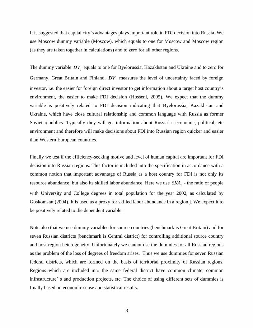
It is suggested that capital city’s advantages plays important role in FDI decision into Russia. We
use Moscow dummy variable (Moscow), which equals to one for Moscow and Moscow region
(as they are taken together in calculations) and to zero for all other regions.
The dummy variable jDV equals to one for Byelorussia, Kazakhstan and Ukraine and to zero for
Germany, Great Britain and Finland. jDV measures the level of uncertainty faced by foreign
investor, i.e. the easier for foreign direct investor to get information about a target host country’s
environment, the easier to make FDI decision (Hosseni, 2005). We expect that the dummy
variable is positively related to FDI decision indicating that Byelorussia, Kazakhstan and
Ukraine, which have close cultural relationship and common language with Russia as former
Soviet republics. Typically they will get information about Russia` s economic, political, etc
environment and therefore will make decisions about FDI into Russian region quicker and easier
than Western European countries.
Finally we test if the efficiency-seeking motive and level of human capital are important for FDI
decision into Russian regions. This factor is included into the specification in accordance with a
common notion that important advantage of Russia as a host country for FDI is not only its
resource abundance, but also its skilled labor abundance. Here we use jSKA - the ratio of people
with University and College degrees in total population for the year 2002, as calculated by
Goskomstat (2004). It is used as a proxy for skilled labor abundance in a region j. We expect it to
be positively related to the dependent variable.
Note also that we use dummy variables for source countries (benchmark is Great Britain) and for
seven Russian districts (benchmark is Central district) for controlling additional source country
and host region heterogeneity. Unfortunately we cannot use the dummies for all Russian regions
as the problem of the loss of degrees of freedom arises. Thus we use dummies for seven Russian
federal districts, which are formed on the basis of territorial proximity of Russian regions.
Regions which are included into the same federal district have common climate, common
infrastructure` s and production projects, etc. The choice of using different sets of dummies is
finally based on economic sense and statistical results.
8

It is obvious that there are a number of other factors that may influence FDI decision into
Russian regions. Especially it concerns regional investment legislation. But as this factor is also
very important for domestic investment and therefore GRP level in regions, its inclusion may
create estimation problems (e.g., multi-collinearity, simultaneity).
4.3. Estimation methods
Our econometric analysis consists of two parts. First we use OLS estimation with parameter
standard errors corrected for heteroskedasticity with White’s heteroskedasticity consistent
covariance estimate. For OLS estimation we exclude from the analysis all zero dependent
observations. Thus our dataset consists only of regions that have at least one firm with FDI from
the mentioned six countries. All the variables in the empirical study (except dummy variables)
appear in natural logarithm form.
Secondly we use Binary Dependent Variable Models for the same specifications. In the model
the dependent variable takes only two values: 1ijY = if there is at least one foreign firm of a
source country i in a region j, and 0ijY = if there are no firms in the region with FDI of the
source country. Thus here all the observations of the sample are present. A simple linear multiple
regression is not now appropriate, since the implied model of the conditional mean places
inappropriate restrictions on the residuals of the model. Furthermore, the fitted value of Y from
OLS regression is not restricted to lie between zero and one. Thus we adopt an estimation
strategy that is designed to handle the specific requirements of binary dependent variables. We
model the probability of observing a value of one as:
(4) Pr( 1 ) ( , ),Y x F x β= =
where x is a vector of explanatory variables, the set of parameters β reflects the impact of
changes in x on the probability to investment. It follows naturally that for Y = 0 we have:
(5) Pr( 0 ) 1 ( , ).Y x F x β= = −
9

F is a continuous, strictly increasing function that takes a real value and returns a value ranging
from zero to one. As Gujarati (2003) notes, the binary choice process has two basic features:
(1) As ix increases, ( 1iP E Y x= = ) increases (decreases) but never steps outside the 0-1 interval,
and (2) the relationship between and iP ix is nonlinear. The choice of the function F determines
the type of binary model. In principle, any proper, continuous probability distribution defined
over the real line will suffice. The most commonly used distributions are the normal cumulative
distribution function and the cumulative logistic function. These give a rise to probit and logit
models, correspondingly (for more technical details see Appendix 2).
5. Results 5.1. Results of OLS estimation
Results of OLS cross-sectional regressions are presented in Table 2. Correlation matrix of the
dependent and explanatory variables is presented in Appendix 3. As jGDP and jAGGL are
highly correlated we use them separately in regression models (3a) and (3b). In regression (3c)
we use dummy variables for Russian districts in order to improve the statistical results of the
model (3b).
All the variables except ln jNR confirm their expected influence on the dependent variable with
statistical significance. However we cannot say much of the unexpected influence of the resource
variable. We note only that resource industries are highly monopolized in Russia and run by one
or few big companies. Thus the total number of foreign firms in such regions depends on some
specific factors.
Results highly support the hypothesis that most FDI into Russian economy at region level are
market seeking as the proxy for market size in a region – ln jGRP – have positive and significant
effect on the dependent variable in all regressions. Secondly, the predictions of gravity model are
supported: gross domestic products of both source countries ( and host regions
( ) and have positive effect on FDI and distance ( ) has negative effect. All
ln ) iGDP
ln iGRP ln ijDIST
10
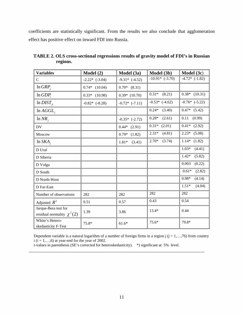
coefficients are statistically significant. From the results we also conclude that agglomeration
effect has positive effect on inward FDI into Russia.
TABLE 2. OLS cross-sectional regressions results of gravity model of FDI’s in Russian regions.
Variables Model (2) Model (3a) Model (3b) Model (3c) C -2.22* (-3.04) -9.31* (-4.52) -10.91* (-3.70) -4.72* (-1.82)
ln jGRP 0.74* (10.04) 0.70* (8.31)
ln iGDP 0.33* (10.98) 0.39* (10.70) 0.31* (8.21) 0.38* (10.31)
ln jiDIST -0.82* (-8.28) -0.72* (-7.11) -0.53* (-4.62) -0.76* (-5.22)
ln jAGGL 0.24* (3.40) 0.47* (5.42)
ln jNR -0.35* (-2.72) 0.28* (2.61) 0.11 (0.99)
DV 0.44* (2.91) 0.31* (2.01) 0.41* (2.92)
Moscow 0.79* (1.82) 2.31* (4.81) 2.23* (5.08)
ln jSKA 1.81* (3.41) 2.70* (3.74) 1.14* (1.82)
D Ural 1.03* (4.41)
D Siberia 1.42* (5.82)
D Volga 0.003 (0.22)
D South 0.61* (2.82)
D North-West 0.98* (4.14)
D Far-East 1.51* (4.04)
Number of observations 282 282 282 282
Adjusted 2R 0.51 0.57 0.43 0.54
Jarque-Bera test for residual normality 2 (2)χ 1.39 3.86 13.4* 0.44
White’s Hetero- skedasticity F-Test
75.8* 61.6* 75.6* 79.8*
Dependent variable is a natural logarithm of a number of foreign firms in a region j (j = 1,…,76) from country i (i = 1,…,6) at year-end for the year of 2002. t-values in parenthesis (SE’s corrected for heteroskedasticity). *) significant at 5% level.
__________________________________________________________________________
11

jDV is also significant and with expected sign. It confirms that common language and culture
ties are positively related to inward FDI. Moscow variable is positive and significant, which
means that the capital city advantage is a rather influential factor of FDI inflows into Russian
economy. Skilled labor abundance variable ln jSKA is also positive and significant and indicates
that FDI into Russian regions are skilled-labor (or human capital) seeking. However according to
the theory of FDI (see, e.g. Markusen, 2002), skilled labor abundant countries tend to have more
outward and less inward FDI in comparison with skilled-labor scarce countries. There are at
least two reasons that help to explain this contradiction. First, it is a well-known fact that labor
force in Russia, including skilled labor, is rather cheap but the theory is based on the fact that
skilled labor is costly and therefore FDI is seeking for cheap unskilled labor. Second, in recent
years there is a FDI tendency in world economy seeking for, instead of cheap resources
(including labor resources), the strategic assets (including human capital). Generally if we look
at the magnitude of coefficients the most important factors are capital city` s advantages, skilled
labor abundance, and the distance between source country and host region.
Almost all regional dummy variables for federal districts are statistically significant. Their
coefficients are called differential intercept coefficients. The coefficients show how the
intercepts differ between federal districts. In equation (3c) the coefficient = -4.7 is the
intercept of the regression for foreign firms in Central district. The intercept of the regression for
foreign firms in the Far Eastern district, for example, equals to (-4.7+1.5), for foreign firms in
the North-Western district – (-4.7+0.98) and so on. If the differential intercept coefficient is
statistically insignificant (like for Volga district in (3c)), than we may accept the hypothesis that
the two regressions (here for foreign firms in Central district and for foreign firms in Volga
district) have the same intercept, that is, the two regressions are concurrent and regional
differences are not present.
1b
4.2. Results of Binary Dependent Variable Models estimation
First, in order to make preliminary conclusions we conduct the dummy variable model for every
explanatory variable. The model is the following:
12
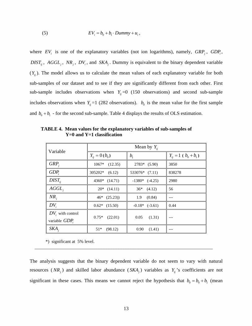
(5) , 0 1i iEV b b Dummy u= + ⋅ +
where is one of the explanatory variables (not ion logarithms), namely, iEV jGRP , ,
,
iGDP
ijDIST jAGGL , jNR , , and iDV jSKA . Dummy is equivalent to the binary dependent variable
( ). The model allows us to calculate the mean values of each explanatory variable for both
sub-samples of our dataset and to see if they are significantly different from each other. First
sub-sample includes observations when =0 (150 observations) and second sub-sample
includes observations when =1 (282 observations). is the mean value for the first sample
and - for the second sub-sample. Table 4 displays the results of OLS estimation.
ijY
ijY
ijY 0b
0b b+ 1
TABLE 4. Mean values for the explanatory variables of sub-samples of Y=0 and Y=1 classification
Mean by ijY
Variable 0ijY = ( ) 0b 1b 1ijY = ( ) 0 1b b+
jGRP 1067* (12.35) 2783* (5.90) 3850
iGDP 305202* (6.12) 533076* (7.11) 838278
ijDIST 4360* (14.71) -1380* (-4.25) 2980
jAGGL 20* (14.11) 36* (4.12) 56
jNR 46* (25.23)) 1.9 (0.84) ---
iDV 0.62* (15.50) -0.18* (-3.61) 0.44
iDV with control
variable iGDP 0.75* (22.01) 0.05 (1.31) ---
jSKA 51* (98.12) 0.90 (1.41) ---
*) significant at 5% level. ________________________________________________________________________
The analysis suggests that the binary dependent variable do not seem to vary with natural
resources ( jNR ) and skilled labor abundance ( jSKA ) variables as ’s coefficients are not
significant in these cases. This means we cannot reject the hypothesis that (mean
ijY
0 0b b b= + 1
13

values for the both sub-samples equal to each other). For the we use also the dummy
variable model with control variable :
iDV
iGDP
(6) . 0 1 2i iDV b b Dummy b GDP u= + ⋅ + ⋅ + i
Without this control variable the just captures the effect of Gross Domestic Product` s
differences between two groups of source countries, namely Post Soviet and West European
countries. Thus the results indicate the preliminary conclusions that all the other factors, namely,
iDV
jGRP , , , iGDP ijDIST jAGGL are important for FDI decision in binary dependent variable
model.
Next we use logit and probit models introduced in Section 4.2 to determine the relative impor-
tance of the factors. We use the same specification of gravity model as for OLS estimation
earlier. However now we use the whole sample. Note that we cannot use Moscow-dummy
variable, as it is always equal to one for all 1ijY = observations. All the explanatory variables
except dummies have been standardized by the following way:
(7) ( )
ist
i
x xx
SD x−
= .
The descriptive summary statistics of the variables used in estimation is presented in
Appendix 4. The results of logit and probit modeling are represented in Table 5.
The results show that the crude form of gravity model’s factors and agglomeration effect play an
important role in FDI decision to invest or not into a particular Russian region as their
coefficients are with expected signs and statistically significant. The coefficients of all the other
factors, namely the stock of natural resources, dummy variable for cultural closeness and skilled
labor abundance, were not statistically significant in most cases as expected from dummy
variable analysis above. Thus we can proceed only with the crude form of gravity model.
14

TABLE 5. Binary Dependent Variable Models for FDI in Russian regions.
Logit Probit Explanatory variables
(2) (3a) (3b) (2) (3a) (3b)
C 2.09* (4.71) 2.10* (3.61) 1.10* (4.62) 0.99* (4.25) 0.91* (3.42) 0.61* ( 4.71) GRPj 6.55* (4.12) 7.42* (3.43) 2.94* (3.24) 3.12 (3.21) GDPi 1.01* (6.74) 1.21* (6.11) 1* (5.4) 0.58* (7.14) 0.67* (6.22) 0.60* (5.62) DISTij -0.41* (-3.23) -0.35* (-2.71) -0.14 (-1) -0.21* (-3.12) -0.21* (-2.60) -0.11 (-0.96) AGGLj 4.11* (4.20) 2.41* (4.42) NRj -0.30 (-1.63) 0.20* (1.93) -0.10 (-1.1) 0.12* (1.92) DV 0.05 (0.42) 0.42 (1.41) 0.24 (1.23) 0.25 (1.34) SKAj 0.53 (1.42) 0.22 (1.62) 0.02 (0.27) 0.12 (1.51) Number of obs. 432 432 432 432 432 432 McFadden R-squared
0.27 0.28 0.16 0.25 0.26 0.16
Akaike IC 0.96 0.96 1.11 0.98 0.99 1.11
LM 2χ -test for Heteroskedasticity
3.14
8.57*
8.55*
7.82*
11.3*
10.8*
Count R-squared 1) 0.18 0.16 0.17 0.19 0.19 0.17
Dependent variable is (no FDI firms) and 0ijY = 1ijY = (at least one FDI firm) in region j (j = 1,…,76) from country i (i = 1,…,6) at year-end for the year 2002. t-values in parenthesis (Huber/White SE). *) significant at 5% level. 1) Count 2R is a measure of goodness of fit in binary regression model which is equal to number of correct predictions / total number of observations (Gujarati, 2003)
________________________________________________________________________________________________
LM test for heteroskedasticity shows that for both cases (logit and probit models) we cannot
reject the hypothesis of heteroskedasticity. Thus we use dummy variables in order to control for
heterogeneity of the source countries. Because the country dummies are highly correlated with
the gross domestic product` s variable of the source countries we exclude the latter from the
equation. We estimate also an Extreme value distribution model as it is a robust alternative that
partly solves heteroskedasticity problem (for details, see Appendix 2). The results are
represented in Table 6.
In all model alternatives all coefficients are statistically significant except the dummy variable
for Germany. LM test rejects the heteroskedasticity alternative. McFadden and Count R-squared
statistics measure the goodness of fit of the model.
15

TABLE 6. Binary Dependent Variable Models for FDI in Russian regions with source countries dummies. Explanatory variables (2a) Logit (2a) Probit (2a) Extreme value C 3.51* (5.61) 1.75* (5.31) 3.11* (7.34) GRPj 7.34* (3.92) 3.32* (3.07) 5.54* (4.81) DISTij -0.42* (-3.22) -0.21* (-3.12) -0.31* (-3.32) D Germany 0.27 (0.54) 0.16 (0.59) 0.24 (0.57) D Byelorussia -1.51* (-3.22) -0.91* (-3.61) -1.10* (-3.01) D Ukraine -1.33* (-3.23) -0.74* (-2.94) -1.12* (-3.21) D Kazakstan -3.32* (-6.22) -1.68* (-6.22) -2.23* (-6.12) D Finland -2.25* (-4.81) -1.28* (-4.91) -1.63* (-4.62) Number of observations 432 432 432 McFadden R-squared 0.31 0.29 0.32 Akaike IC 0.93 0.96 0.92 LM test for Heteroskedasticity 4.78 0.03 2.25 Count R-squared 0.20 0.19 0.19 Dependent variable is (no FDI firms) 0ijY = 1ijY = (at least one FDI firm) in region j (j = 1,…89) from country i (i = 1,…,6) at year-end for the year 2002. t-values in parenthesis (Huber/White SE). *) significant at 5% level. _____________________________________________________________________________________________
We also conclude here (holding other things constant) that Great Britain and Germany tend to
have more firms in Russia than Finland. The Post-Soviet countries Byelorussia and Ukraine tend
to also have more firms in Russia than Kazakhstan. Partly it can be explained by the differences
in gross domestic product of the source countries: large economies tend to make more outward
FDI than small. However Finland, being much larger than Byelorussia and Ukraine, tends to
invest less into Russian economy than Byelorussia and Ukraine. One reason for it is the cultural
closeness of the former Soviet Union republics to Russia. Unfortunately the two variables
employed in the model, gross regional product and distance between host region and source
country, are not directly comparable as they are measured differently.
In order to get a better overview of the marginal effects of independent variables, conditional
predicted probabilities (for more details, see Appendix 4) have been computed using the model
specification 2a-Probit. The results are presented in Table 7. The predicted probabilities tell us
how many regions (in %) may have foreign firms from a particular source country. For instance,
about 99 per cent of those Russian regions, which gross product is about 4500 million euros, will
have German and British firms. Similarly 90% of them will have Finnish firms, 95 % -
16
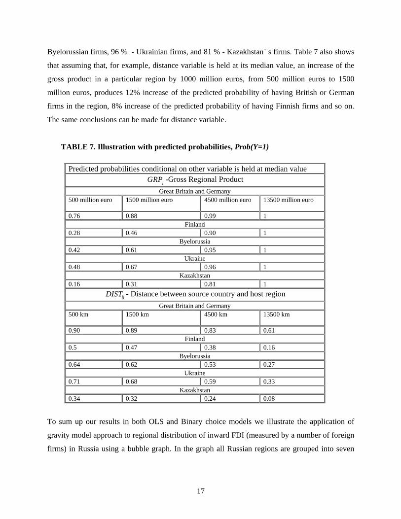
Byelorussian firms, 96 % - Ukrainian firms, and 81 % - Kazakhstan` s firms. Table 7 also shows
that assuming that, for example, distance variable is held at its median value, an increase of the
gross product in a particular region by 1000 million euros, from 500 million euros to 1500
million euros, produces 12% increase of the predicted probability of having British or German
firms in the region, 8% increase of the predicted probability of having Finnish firms and so on.
The same conclusions can be made for distance variable.
TABLE 7. Illustration with predicted probabilities, Prob(Y=1)
Predicted probabilities conditional on other variable is held at median value jGRP -Gross Regional Product
Great Britain and Germany 500 million euro
1500 million euro
4500 million euro 13500 million euro
0.76 0.88 0.99 1 Finland
0.28 0.46 0.90 1 Byelorussia
0.42 0.61 0.95 1 Ukraine
0.48 0.67 0.96 1 Kazakhstan
0.16 0.31 0.81 1
ijDIST - Distance between source country and host region Great Britain and Germany
500 km
1500 km
4500 km
13500 km
0.90 0.89 0.83 0.61 Finland
0.5 0.47 0.38 0.16 Byelorussia
0.64 0.62 0.53 0.27 Ukraine
0.71 0.68 0.59 0.33 Kazakhstan
0.34 0.32 0.24 0.08
To sum up our results in both OLS and Binary choice models we illustrate the application of
gravity model approach to regional distribution of inward FDI (measured by a number of foreign
firms) in Russia using a bubble graph. In the graph all Russian regions are grouped into seven
17

Russian federal districts. The bubbles size reflects the number of foreign firms in each federal
district of the 6 source countries involved in the empirical study.
FIGURE 1. Number of FDI firms, source country distance and level of host region economy activity
Bubble graph of foreign firms presence in Russian Federal Districts in 2002
-10000
100020003000400050006000700080009000
10000
0 2000 4000 6000 8000 10000 12000Average distance from district` s regions to
the source countries of FDI
Ave
rage
GR
P in
the
dist
ricts
Central DistrictNorth-West DistrictSouth DistrictVolga DistrictUral DistrictSiberia DistrictFar Eastern District
In general the graph supports the results of our empirical study. Districts with larger average
gross regional product and smaller average distance from FDI source country tend to have more
foreign firms. The only one evident exception is Ural district where the most FDI is concentrated
in resource industries (Pan-European Institute Report, 2004) that typically have few foreign
firms. Central and North-Western districts have considerably more foreign firms than the other
districts although the differences in the average gross regional product and distance are not so
evident. Agglomeration effects in these districts are evident since the two biggest cities in
Russia – Moscow and Saint Petersburg are located in these district. The relatively large amount
of foreign firms in the Central district can be also explained by the capital city’s advantages.
18
5. Conclusions The paper analyzed the factors affecting the foreign firms presence of six source countries
(namely Great Britain, Finland, Germany, Byelorussia, Ukraine and Kazakhstan) in 76 Russian
regions. The analysis was conducted with a recently compiled cross-sectional data set from the
period of 1998 - 2002 and with different specifications of a gravity model. Two econometric
methods were used: OLS estimation and ML-estimation of Binary Dependent Variable Models.
For OLS estimation we excluded all zero observations. The results suggest that gross products of
host regions and source countries, agglomeration effect, capital city advantages, cultural
closeness and skilled labor abundance are positively related to the number of foreign firms in a
particular Russian region. The distance between host regions and source countries is negatively
related to the dependent variable. As for the resource abundance there is no evidence of an
expected positive influence on the dependent variable. The first possible explanation is the fact
that the resource sector in Russia is highly monopolized. Although it attracts high amounts of
foreign direct investments the number of foreign firms is rather low still in this sector.
In binary choice analysis we include also all zero observations. Thus the dependent variable
equals to one if there is at least one foreign firm in a region of a particular source country and
zero otherwise. The results show that only four factors can be considered to be important in
determining the probability of a foreign firm entering in a particular Russian region. These
factors are gross products of host regions and source countries, distance between them and
agglomeration effect. According to the results the larger is the GDP of a host region and a source
country and the larger is the agglomeration effect of a host region, the higher is the probability of
the region to have foreign firms of this source country. Contrary to this, the larger is the distance
between the host region and the source country the less is this probability.
Thus the major result of the study is that the necessary condition for FDI presence in a particular
Russian region is its economic performance measured by gross regional product. The general
level of regional infrastructure’s development can also be viewed as an important factor of FDI
presence in a region. Regarding the general conclusions we argue that the gravity model
approach can be successfully applied to regional distribution of inward FDI in Russia
irrespectively of the use of a number of foreign firms as a proxy for FDI.
19
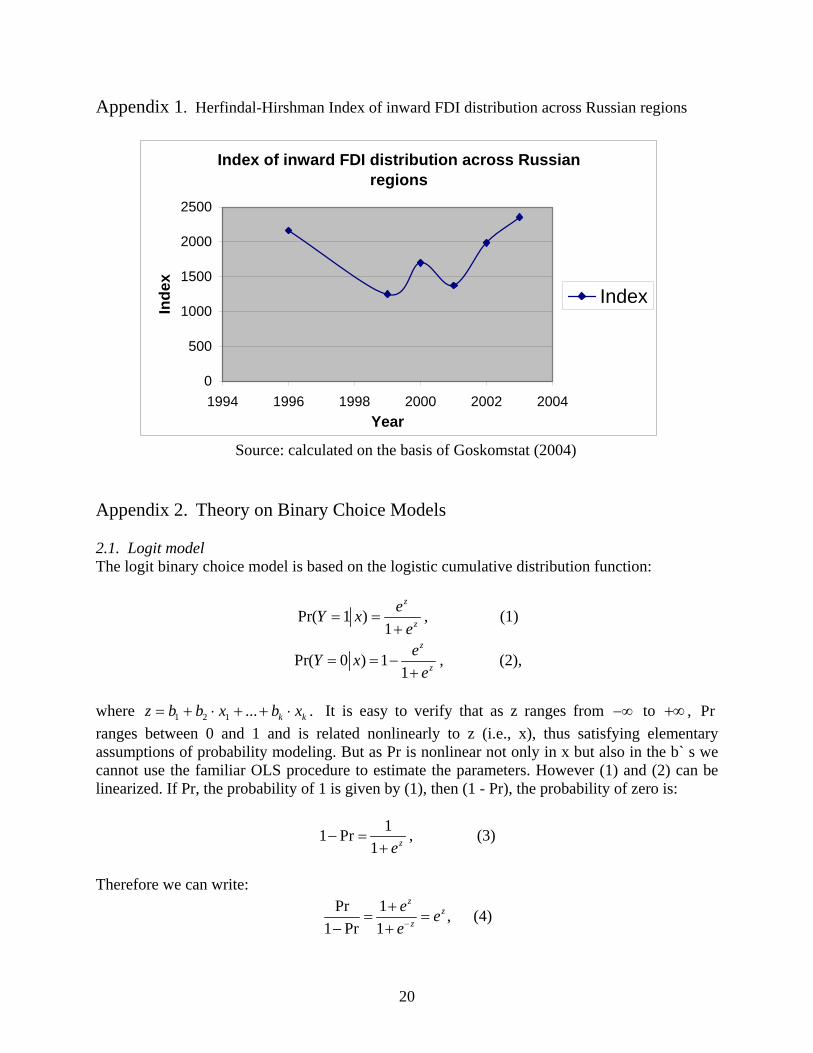
Appendix 1. Herfindal-Hirshman Index of inward FDI distribution across Russian regions
Index of inward FDI distribution across Russian regions
0
500
1000
1500
2000
2500
1994 1996 1998 2000 2002 2004Year
Inde
x
Index
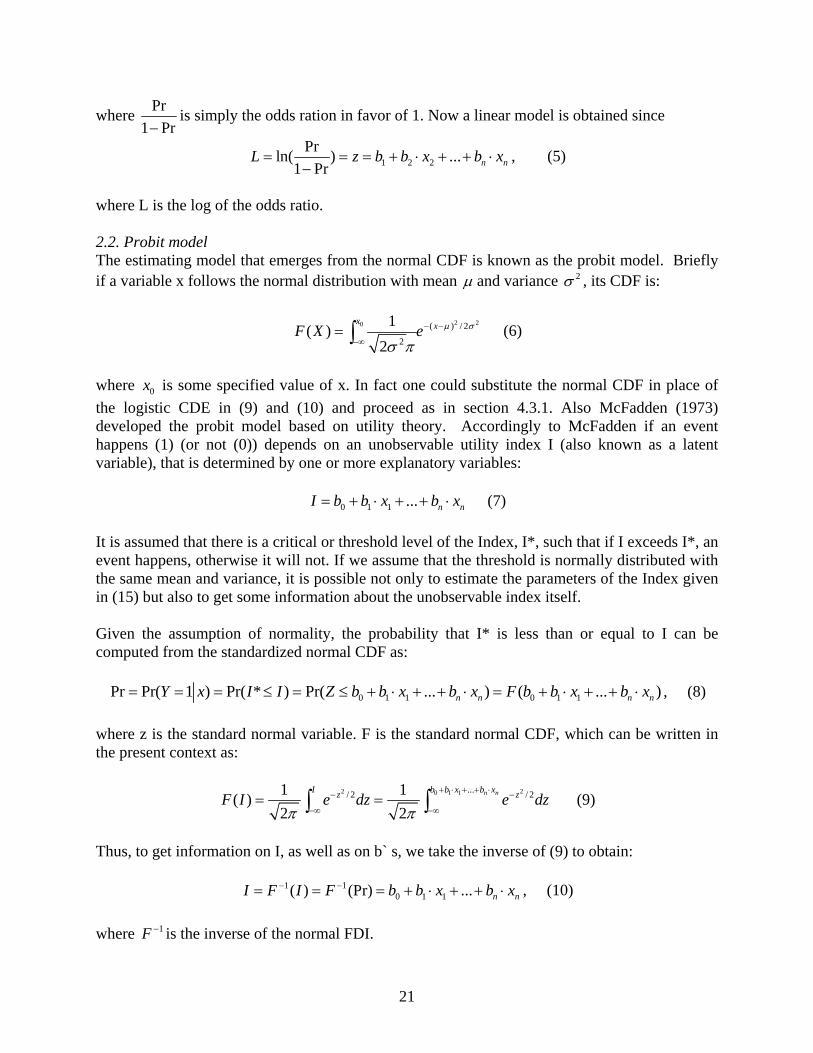
Source: calculated on the basis of Goskomstat (2004) Appendix 2. Theory on Binary Choice Models 2.1. Logit model The logit binary choice model is based on the logistic cumulative distribution function:
Pr( 1 )1
z
z
eY xe
= =+
, (1)
Pr( 0 ) 11
z
z
eY xe
= = −+
, (2),
where . It is easy to verify that as z ranges from to 1 2 1 ... k kz b b x b x= + ⋅ + + ⋅ −∞ +∞ , ranges between 0 and 1 and is related nonlinearly to z (i.e., x), thus satisfying elementary assumptions of probability modeling. But as Pr is nonlinear not only in x but also in the b` s we cannot use the familiar OLS procedure to estimate the parameters. However (1) and (2) can be linearized. If Pr, the probability of 1 is given by (1), then (1 - Pr), the probability of zero is:
Pr
11 Pr
1 ze− =
+, (3)
Therefore we can write:
Pr 1 ,1 Pr 1
zz
z
e ee−
+= =
− + (4)
20
where Pr1 Pr−
is simply the odds ration in favor of 1. Now a linear model is obtained since
1 2 2Prln( ) ...
1 Pr n nL z b b x b x= = = + ⋅ + +−
⋅ , (5)
where L is the log of the odds ratio. 2.2. Probit model The estimating model that emerges from the normal CDF is known as the probit model. Briefly if a variable x follows the normal distribution with mean μ and variance 2σ , its CDF is:
2 20 ( ) / 2
2
1( )2
x xF X e μ σ
σ π− −
−∞= ∫ (6)
where 0x is some specified value of x. In fact one could substitute the normal CDF in place of the logistic CDE in (9) and (10) and proceed as in section 4.3.1. Also McFadden (1973) developed the probit model based on utility theory. Accordingly to McFadden if an event happens (1) (or not (0)) depends on an unobservable utility index I (also known as a latent variable), that is determined by one or more explanatory variables:
0 1 1 ... n nI b b x b x= + ⋅ + + ⋅ (7)
It is assumed that there is a critical or threshold level of the Index, I*, such that if I exceeds I*, an event happens, otherwise it will not. If we assume that the threshold is normally distributed with the same mean and variance, it is possible not only to estimate the parameters of the Index given in (15) but also to get some information about the unobservable index itself. Given the assumption of normality, the probability that I* is less than or equal to I can be computed from the standardized normal CDF as:
0 1 1 0 1 1Pr Pr( 1 ) Pr( * ) Pr( ... ) ( ... )n n n nY x I I Z b b x b x F b b x b x= = = ≤ = ≤ + ⋅ + + ⋅ = + ⋅ + + ⋅ , (8)
where z is the standard normal variable. F is the standard normal CDF, which can be written in the present context as:
2 20 1 1 .../ 2 / 21 1( )2 2
n nI b b x b xz zF I e dz e dzπ π
+ ⋅ + + ⋅− −
−∞ −∞= =∫ ∫ (9)
Thus, to get information on I, as well as on b` s, we take the inverse of (9) to obtain:
1 10 1 1( ) (Pr) ... n nI F I F b b x b x− −= = = + ⋅ + + ⋅ , (10)
where is the inverse of the normal FDI. 1F −
21

2.3. Extreme value model The Extreme value model is based upon the CDF for the Type-I extreme value distribution:
´ `Pr( 1 , ) 1 (1 exp( )) exp( ).i ix xi iy x e eβ ββ − −= = − − − = − (11)
The distribution is skewed. 2.4. Estimating the binary choice models: method of maximum likelihood In all cases for individual data we will have to use a nonlinear estimating procedure based on the method of maximum likelihood. Each observation is treated as a single draw from a Bernoulli distribution (binominal with one draw). The model with success probability F (x` β ) and independent observations leads to the joint probability, or likelihood function:
[ ]1 1 2 20 1
Pr ( , ,..., ) 1 ( ` ) ( ` ),i i
n ny y
ob Y y Y y Y y X F x F xβ β= =
= = = = −∏ ∏ (12)
where X denotes [ ] 1,..., .i i n
x=
The likelihood function for a sample of n observations can be written as:
[ ] [ ]11
( ) ( ` ) 1 ( ` ) .i in
y y
i
L data F x F xβ β −
=
= −∏ β (13)
Taking logs we obtain:
[ ]{ }1
ln ln ( ` ) (1 ) ln 1 ( ` ) .n
i ii
L y F x y F xβ β=
= + − −∑ (14)
The likelihood equation is the following:
1
ln (1 ) 0,(1 )
ni i i
ii i i
y f fL y xF Fβ =
⎡ ⎤−∂= + − ⋅ ⋅⎢ ⎥∂ −⎣ ⎦∑ i = (15)
where if is the density, / ( ` ).idF d x β The choice of a particular form for leads to the empirical model (Gujarati, 2003; Greene, 2003).
iF
2.5. Interpretations of coefficients in logit and probit models In the logit (and in extreme value) model the slope coefficient of a variable gives a change in the log of the odds associated with a unit change in that variable, holding all other variables constant. The slope coefficient for dummy variables indicates a change in the log of the odds associated with the change from 0 to 1 of a variable. In the probit model the slope coefficient of a variable gives a standard deviation change in the predicted probit index associated with a unit change in that variable, holding all other variables
22

constant. For dummy variable, the slope coefficient gives a standard deviation change in the predicted probit index associated with the change from 0 to 1 of a variable. There are several ways of interpreting parameter estimates in probability models (Liao, 1994). In our study we use two of them. First concerns the sign of parameter estimate and its statistical significance. Given a significant statistical test, a positive sign of a parameter estimate suggests the likelihood of the response (event) increases with the level or presence of explanatory variable x, with the other x` s held constant, depending on whether the variable is continuous or dichotomous. Conversely, a negative sign of the estimate suggests that the likelihood of the response decreases with the level or presence of x. Second concerns the predicted probabilities given a set of values in the explanatory variables. Predicted probabilities are intuitively appealing because these give an idea of how likely certain types of events are to affect certain outcomes. Using certain values of the x variables, predicted probabilities are derived by calculating the values of μ :
1
k
k kk
xμ β=
=∑ . (16)
Than we specify η as a linear predictor produced by 1 2, ,..., kx x x . Regardless of the type of model, the set of explanatory variables always linearly produce η , which is a predictor of Y. The relation between η and the x variable is given by:
1
k
k kk
xη β=
= ⋅∑ . (17)
Applying this link function to Equation (16), we specify a logit and probit models:
[ ]log /(1 )η μ μ= − (18) 1( )η μ−= Φ , (19)
where is the inverse of the standard normal cumulative distribution function. 1−Φ Thus we calculate the predicted probabilities e.g. for logit and probit models in the following way:
0 1 1
0 1 1
...
...( 1)1
n n
n n
b b x b x
b b x b x
eProb Ye
+ ⋅ + ⋅
+ ⋅ + ⋅= =+
, (20) 0 1 1Pr ( 1) ( ... )n nob Y b b x b x= = Φ + ⋅ + ⋅ . (21)
If we have many explanatory variables, some of which are categorical, some continuous, it is better to focus on one or two variables of interest and set the values in other variables at their sample means. If one of the two variables that have been selected is discrete and the other is continuous, it is advisable to plot the predicted probability values against the continuous x variable within each category of the discrete variable (Liao, 1994).
23

Appendix 3. Correlation matrix of the dependent and explanatory variables used in OLS estimation
Y GRPj GDPi DISTij AGGLj NRj D1 D2 D3 D4 D5 D6 D7 D8 D9 D10 D11 D12 SKAj DVj MOS Y 1.0 0.6 0.1 -0.1 0.7 -0.2 0.1 0.0 0.0 0.0 -0.1 0.1 0.0 -0.1 -0.1 0.0 0.1 -0.1 0.4 -0.1 0.6 GRPj 0.6 1.0 -0.1 -0.1 0.9 0.1 0.0 0.0 0.0 0.0 0.1 0.1 0.2 -0.1 -0.1 -0.1 -0.1 -0.1 0.5 0.0 0.9 GDPi 0.1 -0.1 1.0 0.3 0.0 0.0 0.7 -0.4 -0.4 -0.3 -0.3 0.0 -0.1 0.0 0.0 0.0 0.0 0.1 0.0 -0.6 0.0 DISTji -0.1 -0.1 0.3 1.0 -0.1 0.2 0.1 -0.2 -0.2 0.0 -0.1 -0.3 0.0 0.3 -0.1 -0.1 -0.2 0.8 0.2 -0.3 -0.1 AGGLj 0.7 0.9 0.0 -0.1 1.0 -0.2 0.0 0.0 0.0 0.0 0.0 0.3 0.0 -0.1 0.0 0.0 -0.1 -0.1 0.4 0.0 1.0 NRj -0.2 0.1 0.0 0.2 -0.2 1.0 0.0 0.0 0.0 0.0 0.1 -0.3 0.4 0.2 -0.1 0.0 0.0 0.0 0.0 0.0 -0.2 D1 Germany 0.1 0.0 0.7 0.1 0.0 0.0 1.0 -0.2 -0.2 -0.2 -0.2 0.0 0.0 0.0 0.0 0.0 0.0 0.0 0.0 -0.4 0.0 D2 Byelorussia 0.0 0.0 -0.4 -0.2 0.0 0.0 -0.2 1.0 -0.2 -0.2 -0.1 0.1 0.0 0.0 0.0 0.0 0.0 0.0 0.0 0.6 0.0 D3 Ukraine 0.0 0.0 -0.4 -0.2 0.0 0.0 -0.2 -0.2 1.0 -0.2 -0.2 0.0 0.0 0.0 0.0 0.0 0.0 0.0 0.0 0.6 0.0 D4 Finland 0.0 0.0 -0.3 0.0 0.0 0.0 -0.2 -0.2 -0.2 1.0 -0.1 -0.1 0.0 0.0 0.0 0.0 0.1 0.0 0.1 -0.3 0.0 D5 Kazakhstan -0.1 0.1 -0.3 -0.1 0.0 0.1 -0.2 -0.1 -0.2 -0.1 1.0 -0.1 0.1 0.1 0.0 0.0 0.0 -0.1 0.0 -0.2 0.0 D6 Central 0.1 0.1 0.0 -0.3 0.3 -0.3 0.0 0.1 0.0 -0.1 -0.1 1.0 -0.2 -0.2 -0.3 -0.2 -0.3 -0.2 -0.1 0.1 0.3 D7 Ural 0.0 0.2 -0.1 0.0 0.0 0.4 0.0 0.0 0.0 0.0 0.1 -0.2 1.0 -0.1 -0.1 -0.1 -0.1 -0.1 0.1 0.0 0.0 D8 Siberia -0.1 -0.1 0.0 0.3 -0.1 0.2 0.0 0.0 0.0 0.0 0.1 -0.2 -0.1 1.0 -0.2 -0.1 -0.2 -0.1 0.0 0.0 -0.1 D9 Volga -0.1 -0.1 0.0 -0.1 0.0 -0.1 0.0 0.0 0.0 0.0 0.0 -0.3 -0.1 -0.2 1.0 -0.2 -0.2 -0.1 -0.3 0.0 -0.1 D10 South 0.0 -0.1 0.0 -0.1 0.0 0.0 0.0 0.0 0.0 0.0 0.0 -0.2 -0.1 -0.1 -0.2 1.0 -0.1 -0.1 0.1 0.0 0.0 D11 North West 0.1 -0.1 0.0 -0.2 -0.1 0.0 0.0 0.0 0.0 0.1 0.0 -0.3 -0.1 -0.2 -0.2 -0.1 1.0 -0.1 0.1 0.0 -0.1 D12 Far East -0.1 -0.1 0.1 0.8 -0.1 0.0 0.0 0.0 0.0 0.0 -0.1 -0.2 -0.1 -0.1 -0.1 -0.1 -0.1 1.0 0.2 -0.1 0.0 SKAj 0.4 0.5 0.0 0.2 0.4 0.0 0.0 0.0 0.0 0.1 0.0 -0.1 0.1 0.0 -0.3 0.1 0.1 0.2 1.0 0.0 0.4 DVj -0.1 0.0 -0.6 -0.3 0.0 0.0 -0.4 0.6 0.6 -0.3 -0.2 0.1 0.0 0.0 0.0 0.0 0.0 -0.1 0.0 1.0 0.0 MOSCOW 0.6 0.9 0.0 -0.1 1.0 -0.2 0.0 0.0 0.0 0.0 0.0 0.3 0.0 -0.1 -0.1 0.0 -0.1 0.0 0.4 0.0 1.0
Appendix 4. Descriptive statistics of the dependent and explanatory variables used in Binary Choice Models
Y DISTji jGRP iGDP jSKA jAGGL jNR
Mean 0.7 3386.4 2887.1 654416.1 51.9 43.4 46.8
Median 1.0 2553.0 1390.2 89638.2 51.5 23.4 40.0
Maximum 1.0 12736.0 51307.9 2110400.0 67.6 1117.1 94.1
Minimum 0.0 323.0 128.8 12965.4 40.4 0.8 9.1
Std. Dev. 0.5 2742.6 6450.8 864068.3 5.8 129.9 21.5
Skewness -0.7 1.5 6.2 0.8 0.2 7.9 0.5
Kurtosis 1.4 4.6 45.4 1.8 2.7 65.2 2.1
Jarque-Bera test 75.3 200.3 35042.6 73.0 4.2 74058.8 28.6
24

References Anderson J.E., 1979, A Theoretical Foundation for the Gravity Equation, American economic Review, 69, 106-116. Barrel R., Pain. N., 1999, Trade restraints and Japanese direct investment flows. European Economic Review, 43, 29-45. Bevan A., Estrin S., 2004, The determinants of foreign direct investment into European transition economics, Journal of Comparative Economics, 32, 775-787. Bergstrand J.H., 1985, The Gravity Equation in International Trade: Come microeconomic Foundations and Empirical Evidence, The Review of Economics and Statistics, 67, 474-481. Breitung J., 2002, A parametric approach to the estimation of cointegration vectors in panel data. Unpublished manuscript. Humboldt University, Berlin. Broadman H., Recanatini F., 2004, Where does all the foreign direct investment go in Russia? Draft paper. Buch C.M., Kokta R.M., Piazolo D., 2003, Foreign direct investment in Europe: Is there redirection from the South to the East? Journal of Comparative economics, 31, 94-109. Deardorff A.V., 1995, Determinants of Bilateral Trade: Does gravity work in a Neoclassical World? The Regionalization of the World Economy, Jeffrey A. Frankel, ed., University of Chicago Press. Dunning J., 1958, American Investment in British Manufacturing Industry. Georg Allen and Unwin, London. Casson M.C., 1987, The firm and the market: studies in multinational enterprises and the scopes of the firm. Oxford: Blackwell. Chakrabarti A., 2003, A theory of the spatial distribution of foreign direct investment. International Review of Economics & Finance, Volume 12, Issue 2, 149-169. Ethier W., 1986, The multinational firm. Quarterly Journal of Economics, 101, 805-833. & Markusen J.R., 1996, Multinational firms, technology diffusion and trade. Journal of International economics, 41, 1-28. & Markusen J.R., 1991, Multinational firms, technology diffusion and trade. NBER Working Paper, No. 3825. Frenkel M., Funke K., Stadtmann G., 2004, A panel analysis of bilateral FDI flows to emerging economies. Economic Systems 28, 281-300. Greene, W.H., 2003, Econometric analysis, 5th ed., prentice-Hall, New Jersey. Gujarati D.N., 2003, Basic Econometrics, McGrawHill, United State Military Academy, West Point. Haufler A., Wooton I., 1999, Country size and Tax competition for foreign direct investment. Scandinavian Journal of economics, 101, 631-649. Hosseini H., 2005, An economic theory of FDI: A behavioral economics and historical approach, The Journal of Socio-Economics 34, 528-541. Kristiansdottir H., 2004, Determinants of Exports and Foreign Direct Investment in a Small Open Economy, Ph. D. Dissertation, University of Iceland, Faculty of Business and Economics. Linnemann H, 1966, An econometric study of international trade flows, Amsterdam: North- Holland. Liao T.F. 1994, Interpreting probability models: logit, probit, and other generalized linear models, SAGE publications.
25

Pöyhönen P., 1963, ”A Tentative Model for the Volume of Trade between Countries”, Weltwirtschaftliches Archiv, 90 (1), pp.93-100. Rugman A.M., 1986, New theories of the multinational enterprisers: an assessment of internalization theory. Bulletin of Economics, 38. Russia` s Regions yearbook, Goskomstat, 2004 Tinbergen J., 1962, Shaping the World Economy: Suggestions for an International Economic Policy, New York, The Twentieth Century Fund. UNCTAD, 2003, Statistical Yearbook UN, New York. . Valiulin X.X., Shakirova E.R., 2004, Heterogeneity of investment space in Russia: regional aspect, Forecasting problems, 1. Williamson O.E., 1981, The modern corporation: origins, evolution, attributes. Journal of Economic Literature, 19, 161-175. Woodward D.P., 1992, Location determinants of Japanese manufacturing start-ups in the United State. Southern Economic Journal, 58, 690-708. Yeaple, S.R., 2001, The determinants of US outward foreign direct investment: market access versus comparative advantage. Working paper. Distance calculator: http://truckmarket.ru/tc.php Foreign Direct Investment into and from Russia: report, 2004, Pan-European Institute: www.tukkk.fi/pei/e
26