testing algorithms and software -...
TRANSCRIPT
NPL REPORT DEM-ES 003
Software Support for Metrology – Good Practice Guide No. 16 Testing Algorithms and Software
R M Barker, P M Harris and L Wright
Not Restricted
December 2005
Version 1.0
National Physical Laboratory | Hampton Road | Teddington | Middlesex | United Kingdom | TW11 0LW
Switchboard 020 8977 3222 | NPL Helpline 020 8943 6880 | Fax 020 8943 6458 | www.npl.co.uk

Software Support for Metrology Good Practice Guide No 16 Testing Algorithms and Software
R M Barker, P M Harris and L Wright National Physical Laboratory
Teddington, Middlesex, United Kingdom. TW11 0LW
December 2005
Abstract
Since their inception, the SSfM programmes have worked on testing of software used in metrology: developing methodologies and applying them to testing our own software and testing packages used in processing measurement data. The success of the testing methodologies is shown by the errors that have been found in widely-used packages, errors that we have been able to trace to errors in the implementations of numerical routines.
This guide consolidates and summarises the methodologies for testing software for discrete and continuous modelling, and for testing the underlying algorithms. This guide draws on a number of guides and reports from the previous SSfM programmes, and uses examples from those documents to illustrate the methodologies.
Version 1.0

© Crown copyright 2005
Reproduced with permission of the Controller of HMSO and Queens Printer for Scotland
ISSN 1744–0475
Extracts from this guide may be reproduced provided the source is acknowledged and the extract is not taken out of context
We gratefully acknowledge the financial support of the UK Department of Trade and Industry (National Measurement System Directorate)
Approved on behalf of the Managing Director, NPL by Jonathan Williams, Knowledge Leader for the Electrical and Software team
National Physical Laboratory
Teddington, Middlesex, United Kingdom. TW11 0LW

Table of Contents 1. Introduction .............................................................................................. 1 1.1 Structure of this Guide .....................................................................................................1 1.2 Rationale for the Guide ....................................................................................................1
1.2.1 Scope ....................................................................................................................1 1.2.2 Effects producing inexactness ..............................................................................2 1.2.3 Mathematical and statistical models .....................................................................2 1.2.4 Fitness for purpose................................................................................................3 1.2.5 Testing framework................................................................................................3 1.2.6 Different issues for discrete and continuous modelling........................................5
1.3 Relationship to other SSfM documents............................................................................6 1.3.1 Best- and Good-Practice Guides and important reports .......................................6 1.3.2 Reports and other SSfM documents......................................................................7
1.4 Resources .........................................................................................................................8 1.5 Acknowledgements ..........................................................................................................8 2. Glossary.................................................................................................... 9 3. Overview of Approach........................................................................... 12 3.1 Understanding the testing problem ................................................................................12 3.2 Applying analysis to the testing problem.......................................................................14 3.3 Applying reference pairs to the testing problem ............................................................14
3.3.1 Specification of reference pairs ..........................................................................14 3.3.2 Calculation of reference pairs .............................................................................15 3.3.3 Specification of quality metrics ..........................................................................18
3.4 Complementary checks ..................................................................................................23 3.4.1 Checking consistency of functions .....................................................................23 3.4.2 Checking continuity of functions........................................................................23 3.4.3 Checking against tabulated or other values ........................................................23 3.4.4 Checking solution characterisations ...................................................................23
3.5 Simulation ......................................................................................................................24 3.6 Presentation and interpretation of results .......................................................................24 4. Discrete Modelling Example: Gaussian Peak Fitting.......................... 26 4.1 Understanding the testing problem ................................................................................26
4.1.1 Target computational aim ...................................................................................26 4.1.2 Test computational aim.......................................................................................26 4.1.3 Implementation of the test software....................................................................27
4.2 Applying analysis to the testing problem.......................................................................27 4.2.1 Mathematical analysis of the computational aims ..............................................27 4.2.2 Numerical analysis of the test software ..............................................................28
4.3 Applying reference pairs to the testing problem ............................................................29 4.3.1 Specification of reference pairs ..........................................................................29 4.3.2 Calculation of reference pairs .............................................................................29 4.3.3 Specification of quality metrics ..........................................................................30
4.4 Simulation ......................................................................................................................30 4.5 Presentation and interpretation of results .......................................................................31
i

5. Continuous Modelling Example: Heat Transfer .................................. 36 5.1 Understanding the testing problem ................................................................................36
5.1.1 Target computational aim ...................................................................................36 5.1.2 Test computational aim.......................................................................................37 5.1.3 Implementation of the test software....................................................................37
5.2 Applying analysis to the testing problem.......................................................................38 5.2.1 Mathematical analysis of the computational aims ..............................................38 5.2.2 Numerical analysis of the test software ..............................................................39
5.3 Applying reference pairs to the testing problem ............................................................39 5.3.1 Specification of reference pairs ..........................................................................41 5.3.2 Calculation of reference pairs .............................................................................42 5.3.3 Specification of quality metrics ..........................................................................43
5.4 Complementary checks ..................................................................................................44 5.5 Simulation ......................................................................................................................44 5.6 Presentation and interpretation of results .......................................................................44 6. References.............................................................................................. 52
ii
Testing Algorithms and Software NPL Report DEM-ES 003
1. Introduction This Guide is produced by the Software Support for Metrology programme, which is a DTI programme giving support to measurement scientists in mathematics and software. Since their inception, the SSfM programmes have included work to support the testing of software used in metrology: developing methodologies and applying them to testing NPL’s own software and software packages developed elsewhere for processing measurement data. The success of the testing methodologies is shown by the poor performance that has been identified in some widely-used packages, a problem that we have been able to trace to poor choices of numerical routine [15].
This Guide consolidates and summarises the methodologies for testing software for discrete and continuous modelling, and for testing the underlying algorithms. This Guide draws on a number of guides and reports from the previous SSfM programmes, and uses examples from those documents to illustrate the methodologies.
1.1 Structure of this Guide This Guide describes a common approach to testing and demonstrates many aspects of the testing approach through two examples. The common techniques for testing are described, and the two examples show how these techniques are applied in discrete and continuous modelling problems. Further details of the testing approach and techniques are referenced in other SSfM documents.
The structure of the Guide is as follows:
• The background and philosophy to the approach in this guide
• A glossary of terms used repeatedly throughout the Guide
• An overview of techniques common to all problems
• An example of testing for discrete modelling problems
• An example of testing for continuous modelling problems
1.2 Rationale for the Guide
1.2.1 Scope The focus of this document is on giving guidance on methods for investigating the fitness for purpose of a software implementation of an algorithm to solve a specified, and well-defined, mathematical model. The software is referred to as the test software1, the algorithm implemented by the test software as the test algorithm, and the (well-defined) specification of the mathematical model as the computational aim. The Guide brings together previous work on techniques for algorithm and numerical software testing, applied to discrete and continuous modelling software.
The Guide is intended for both users and developers of software for solving discrete and continuous modelling problems. It addresses the requirements placed on users and developers to demonstrate that software is fit for its intended purpose. In addition, the Guide is intended to assist Quality Managers by providing information on how to monitor and control the acceptability of software as part of measurement, production and inspection systems.
This Guide should be considered in the context of Software Support for Metrology Best-Practice Guide No 1: Validation of software in measurement systems [32]. That guide describes an overall approach to validation of software, defining a number of techniques that 1 This is to be distinguished from software that may be used to undertake the testing.
Page 1 of 53

NPL Report DEM-ES 003 Testing Algorithms and Software
can be used to ensure the fitness for purpose for a (measurement) system that includes software. The particular techniques to be applied are determined by reference to the complexity of the software and the intended use of the software. Testing is a core element of validation and testing of numerical correctness is important to all measurement software. Therefore, this Guide provides a method of implementing one of the validation techniques defined in Best-Practice Guide No 1.
1.2.2 Effects producing inexactness As part of the process of using software to obtain a solution to a problem in metrology, there are a number of effects that produce inexactness in the (measurement) result delivered by the software. These include:
• Modelling effects, arising from limitations of the chosen mathematical model to represent faithfully the physical problem required to be solved.
• Algorithm effects, arising from limitations of a chosen algorithm to deliver a solution to the mathematical model (above).
• Numerical effects, arising from the use of a software implementation of the algorithm (above) to compute the solution.
• Data effects, arising from inexactness in data values (including measurement data, reference constants, calibration information, initial and boundary data, etc.) that define the particular instance of the physical problem required to be solved.
We use the term Validation for the generic activity that encompasses consideration of all these effects within this process. It is an activity that is important to metrology and is driven by the requirement to demonstrate the correctness and traceability of a measurement result.
Traceability is the documentation of a calibration chain, supported by associated uncertainties, between an instrument and a primary standard. For the software used to deliver a measurement result, traceability is the documentation of all aspects in the process of development, implementation and testing of a model in software so that each stage in the process can be understood, checked and reproduced.
These are the effects that will produce inexactness in the numerical calculation: there are, of course, many other software effect that will cause numerical software to go wrong. The general approach to testing and validation of numerical software in the context of a general (measurement) system is the subject of Software Support for Metrology Best-Practice Guide No 1 [32], referred to above.
1.2.3 Mathematical and statistical models The most difficult effect to investigate is that associated with the mathematical model. Generally, the model is chosen on the basis of the user’s understanding and knowledge of the physical problem. Although there may be established “tried and tested” models available for particular problems, there is often an aspect of subjectivity in choosing the model. Generally, the model can always be expected to incorporate approximations to the physical problem. Sometimes these approximations will be deliberate, and are introduced to generate mathematical models that are tractable or efficient to solve. Examples include assuming linearity, symmetry, homogeneity, exactness of data, etc.
Investigating and quantifying data effects is the subject of uncertainty evaluation, based on a statistical model. The measurement result is obtained by evaluating the mathematical model used to describe the measurement problem for estimates of the values of the data that define the particular instance of the problem required to be solved. The uncertainty associated with the measurement result is evaluated in terms of the model and the uncertainties associated with those estimates (or other information concerning the inexactness of the estimates).
Page 2 of 53

Testing Algorithms and Software NPL Report DEM-ES 003
1.2.4 Fitness for purpose Validation is used to demonstrate that the use of an approximate mathematical model, an approximate algorithm to solve the model, and software as an implementation of the approximate algorithm, are fit for purpose. In this context, fitness for purpose may be described qualitatively, e.g., the solution demonstrates a physical property such as conservation of energy.
Often validation techniques are unable to distinguish the contributions made by the different effects. For example, if it is found that the solution delivered by software for solving a measurement problem fails to satisfy a property expected of a solution to that problem (examples include conservation of energy, asymptotic behaviour, etc.) then it can be difficult to know (without further information) whether the failure is associated with the model, the algorithm, the software implementation or a combination of these.
Fitness for purpose can also mean that the effects arising from the use of the approximate mathematical model, approximate algorithm, etc. are quantitatively small compared to those effects arising from the data, the latter described by an uncertainty. In cases that the use of an approximate mathematical model, approximate algorithm, etc. are shown not to be fit for purpose it is necessary either to correct for these effects, e.g., to use a more sophisticated mathematical model, algorithm, etc., or to quantify the effects and include them as additional contributions in the uncertainty evaluation.
1.2.5 Testing framework The development of software for solving a numerical problem is divided into the development of an algorithm for solving the problem and a translation of the algorithm into code. This subdivision is reflected in testing: if the test algorithm is known, we can perform tests on the algorithm and tests on the software relative to the algorithm. We can also test algorithms on their own, so that algorithms can be seen as fit for purpose for a class of problems, without singling out any particular piece of software.
In circumstances where the test algorithm is known, consideration may be given to answering the questions “how good is the test algorithm for solving the mathematical model?” and “how good is the test software for delivering a result for the test algorithm?” In this work, these are the questions addressed by the activities of, respectively, algorithm testing and numerical software testing.
The framework for algorithm testing used in this Guide is based on comparison within a matrix of different manifestations of the problem/calculation (Figure 1.1). The vertical axis is the degree of abstraction of the calculation from (mathematical) computational aim, through algorithm, to software; the other axis is the degree of approximation with which the calculation solves the problem. The different techniques for algorithm testing can be seen as comparisons along one axis or the other, and some comparisons are “diagonal”, e.g. comparing an implementation of an approximate algorithm with the computational aim.
Page 3 of 53

NPL Report DEM-ES 003 Testing Algorithms and Software
(Test) Algorithm
(Test) Software
(Test) Computation aim
(Reference) Algorithm
(Reference) Software
(Target) Computation aim
Figure 1.1 Framework for algorithm testing.
The key techniques in algorithm testing are peer review of the (documented) algorithm and numerical software testing of implementations based on the algorithm. When testing an algorithm independent of its implementation, numerical software testing may still be useful. A “reference” implementation of the algorithm may be developed that accurately performs the algorithm (but presumably at some cost in terms of efficiency); the reference implementation can then be used for comparison with other implementations or for testing. It may also be possible to analyse the results of numerical software testing to determine errors that are contributed by a poor choice of algorithm and those that are contributed by the implementation.
It is common to use generic algorithms and generic (commercial off the shelf) software implementations of those algorithms to solve a (wide) variety of mathematical models. Examples include using a linear least-squares solver to represent experimental data by a linear calibration curve, and using the boundary element method (with linear elements) to solve the Helmholtz equation. If these generic components can be shown to be fit for purpose, the metrologist is left to concentrate on how modelling effects impact on the solution to the measurement problem.
In circumstances where details of the test algorithm are not known (as can be typical when using commercial off the shelf software), all that can be done is to investigate how good the test software is at delivering a solution to the problem specified by the computational aim. In this case, the software is regarded as a black box, and its testing addresses the question “how good is the test software for solving the mathematical model?” In contrast to black-box testing, testing that uses knowledge of the algorithm or implementation to design the tests, yet only interacts with the software through its inputs and output, is termed grey-box. White-box testing, based on internal access to the software, is not part of the methodology of this guide.
In the case of commercial off the shelf software users may also want to draw some general conclusions about the software, e.g. how well it solves a class of problems, rather than a specific test problem(s). Some techniques for the testing of algorithms can be applied even when the algorithm employed in software is not known; numerical software testing may reveal which algorithm is probably used by the software and, if appropriate, further testing could be used to test that algorithm.
Page 4 of 53
Testing Algorithms and Software NPL Report DEM-ES 003
1.2.6 Different issues for discrete and continuous modelling Although the Guide discusses concepts and techniques that are generic to both discrete and continuous modelling problems, descriptions of particular techniques for the two types of problem are kept mostly separate.
• One reason for this is that the audiences for the material relating to the two types of problem are generally different.
• A second reason is that there are often different considerations for each.
For example, some software for solving continuous modelling problems (particularly commercial off the shelf software) is aimed at solving specific classes of physical problem (e.g., thermal, acoustic, structural, etc.) rather than general models defined by arbitrary (systems of) differential equations. Consequently, reference problems for testing such software must be constructed to represent these classes of physical problem, and indeed it may be difficult to express the reference problems in terms of (systems of) differential equations.
In contrast, software for solving discrete modelling problems is invariably developed to solve general models, e.g., a linear least-squares solver may be used to determine any linear calibration function from measurement data, and the specification of the model in terms of mathematical equations is usually possible.
• A further reason is that the solutions obtained from software for solving continuous modelling problems are (almost) always subject to algorithm error as a consequence of the discretisation of the problem that is a part of the algorithms used by such software.
In contrast, there are many discrete modelling problems for which algorithms exist for delivering (mathematically) correct solutions and the concern is with the numerical properties of implementations of those algorithms.
• A final reason is that challenging reference problems with known solutions are rare for many types of continuous modelling.
In general, if a continuous modelling problem has an analytic solution, the problem is likely to be either simple or far removed from real-world problems. Hence it can be difficult to create reference problems that stretch the software’s capabilities and test its suitability for application to real metrology problems.
The Guide assumes primarily that the software is available as a black box, though consideration is given to how knowledge about the test algorithm and its implementation in the test software can contribute to the testing process. The aim of the testing is, predominantly, to investigate the ability of the software to generate a particular result rather than to check whether the software implements a particular algorithm. This is consistent with the way most proprietary (commercial off the shelf) software for discrete and continuous modelling is used.
Page 5 of 53
NPL Report DEM-ES 003 Testing Algorithms and Software
1.3 Relationship to other SSfM documents
1.3.1 Best- and Good-Practice Guides and important reports The following companion best- and good-practice guides and reports contain relevant material:
SSfM BPG1 Validation of software in measurement systems – Testing of software, and determination of fitness for purpose of software packages, is a major element of software validation. [32]
SSfM BPG4 Discrete modelling and experimental data analysis – Software to solve discrete modelling problems form an important class to be tackled by the software testing methodology. The guide also includes techniques for the validation of discrete models. [5]
In the context of testing, BPG 4 covers validation of discrete model effects.
SSfM GPG5 Guide to EUROMETROS – The EUROMET Repository of Software (EUROMETROS) contains measurement software that has been tested using the methodology in this guide and contains test data sets for testing implementations of data fitting software. [4]
SSfM BPG6 Uncertainty evaluation – Software to support evaluation of uncertainties in measurement problems is also a class of software that can be tackled using the software testing methodology. [19]
In the context of testing, BPG6 covers aspects of fitness for purpose and validation of data effects.
SSfM BPG7 Development and testing of spreadsheet applications – The testing methodology is applicable to the testing of spreadsheet applications; but perhaps more importantly, the testing methodology has revealed some shortcomings in popular spreadsheet packages, emphasising the need for developers of spreadsheet applications to test their applications, partly to ensure the fitness for purpose of the underlying spreadsheet package. [2]
SSfM BPG11 Numerical analysis for algorithms design in metrology – Numerical analysis of the intended computation is a key component in the methodology for testing algorithms and software. [20]
SSfM BPG12 Guide for test and measurement software – Software testing is a key component in the development of measurement software; the methodology in this guide is equally important for determining the fitness for purpose of mathematical library software that is used as the basis for particular measurement software applications. [12]
CMSC 29/03 Model Validation in Continuous Modelling – This report provides general advice about the process of validation and describes methods and techniques that can be used for validating continuous models, many of which have been developed to address problems specific to continuous modelling. [23]
In the context of testing, CMSC 29/03 covers validation of continuous model effects.
Page 6 of 53
Testing Algorithms and Software NPL Report DEM-ES 003
1.3.2 Reports and other SSfM documents This Guide is based on material developed in the first two SSfM programmes:
SSfM-2 2001-2004
• Testing Algorithms in Standards and METROS, CMSC 18/03 [3] • The Comparison of Algorithms for the Assessment of Type A1 Surface Texture
Reference Artefacts, CMSC 33/03 [26]
• Testing the Numerical Correctness of Software, CMSC 34/04 [21]
• Testing Methods of Java Libraries, CMSC 35/04 [8]
• Testing Continuous Modelling Software, CMSC 41/04 [24]
• Testing Continuous Modelling Software: Three Case Studies , CMSC 42/04 [25]
• Testing Algorithms for Free-Knot Spline Approximation, CMSC 48/04 [28]
SSfM-1 1998-2001
• The Design and Use of Reference Data Sets for Testing Scientific Software (paper) [16]
• A Methodology for Testing Spreadsheets and Other Packages Used in Metrology, CISE 25/99 [13]
• Testing Spreadsheets and Other Packages Used in Metrology, a Case Study, CISE 26/99 [14]
• Testing Spreadsheets and Other Packages Used in Metrology – Testing the Intrinsic Functions of Excel, CISE 27/99 [15]
• Testing Spreadsheets and Other Packages Used in Metrology: Testing the Intrinsic Functions of Mathcad, CMSC 05/00 [6]
• Testing Spreadsheets and Other Packages Used in Metrology: Testing the Intrinsic Functions of S-Plus, CMSC 06/00 [7]
• Testing Spreadsheets and Other Packages Used in Metrology: Testing Functions for the Calculation of the Standard Deviation, CMSC 07/00 [17]
• Testing Spreadsheets and Other Packages Used in Metrology: Testing Functions for Linear Regression, CMSC 08/00 [18]
Page 7 of 53
NPL Report DEM-ES 003 Testing Algorithms and Software
1.4 Resources These web-based resources may also provide useful material for numerical software testing.
• Tools for Evaluating Mathematical and Statistical Software math.nist.gov/stssf/
• NIST statistical reference data sets www.itl.nist.gov/div898/strd/
• Resources for Improving Accuracy in Statistical Software www.hmdc.harvard.edu/numerical_issues/
• A Web-Based Library for Testing the Performance of Numerical Software www.polymath-software.com/library/
• NAFEMS benchmarks for finite element calculations http://www.nafems.org/ shop/commerce.cgi?product=Benchmark_Tests&cart_id=3096322.14962
• Tests of the quality of random number generators: TestU01 (including Small Crush, Crush and Big Crush) www.iro.umontreal.ca/~simardr/testu01/tu01.html
There are also on-line resources from NPL and SSfM projects.
• SSfM data generators for calculations in discrete modelling www.npl.co.uk/ssfm/theme2/rds/
• SSfM on-line testing services for calculations in discrete modelling www.npl.co.uk/ ssfm/ssfm3/theme3/numerical_software_testing/project3_2/milestone3/
• EUROMETROS www.eurometros.org/
• SOFTGAUGES website that provides reference software and reference data for testing software for the evaluation of surface texture parameters http://161.112.232.32/softgauges/default.htm
Also useful resources are the books
• Accuracy and Stability of Numerical Algorithms, by Nick Higham [30]
• Statistics Software Qualification: Reference Data Sets, edited by B.P. Butler, M.G. Cox, S.L.R. Ellison, and W.A. Hardcastle [10]
and papers in Quality Of Numerical Software: Assessment And Enhancement – Oxford 1996, including:
• Testing linear algebra software Nick Higham [29]
• A methodology for testing classes of approximation and optimisation software Bernard Butler, Maurice Cox, Alistair Forbes, Simon Hannaby and Peter Harris [9]
1.5 Acknowledgements This Guide was produced under the Software Support for Metrology (SSfM) programme, which is managed behalf of the DTI by the National Physical Laboratory. For more information on the SSfM programme visit the website at www.npl.co.uk/ssfm or contact the programme manager Mr Bernard Chorley (phone +44 20 8943 7050, email: [email protected], National Physical Laboratory, Hampton Road, Teddington, Middlesex, UK TW11 0LW).
This Guide relies heavily on the work that lead to the SSfM documents listed in section 1.3 and we gratefully acknowledge the authors of those documents.
Page 8 of 53

Testing Algorithms and Software NPL Report DEM-ES 003
2. Glossary Absolute error The magnitude of the difference between test and reference
results corresponding to a reference problem.
Algorithm effect Effect on the correctness of a measurement result arising from limitations of a chosen algorithm to deliver a solution to the problem specified by a computational aim.
Algorithm testing Investigating the extent to which using a (test) algorithm to solve the problem specified by a test computational aim delivers a solution to the target problem (as specified by the target computational aim).
Black-box testing Testing of software using solely the inputs and output of the software – not based on knowledge of the algorithm, or the manner in which that algorithm is implemented.
Computational aim An unambiguous specification of the problem solved by software, for example in the form of the inputs to, and outputs from, the software and the mathematical model relating the inputs and the outputs.
Data effect Effect on the correctness of a measurement result arising from the inexactness of data values (including measurement data, reference constants, calibration information, initial and boundary data, etc.).
Discretisation error The error caused by approximating a continuous differential equation with a numerical solution. Usually considered as the difference between an analytic solution and an idealised numerical solution, without considering the effects of finite precision arithmetic.
Domain tests Tests in which the mathematical formulation of the problem is held fixed, but the domain on which the problem is solved is varied.
Fit for purpose Software that satisfies a claim about its numerical performance, for example expressed in terms of an absolute or relative error, or a performance measure.
Grey-box testing Testing of software using the inputs and output of the software – but where the testing strategy is based on a knowledge of the algorithm and how that algorithm is implemented.
Mathematical equivalence (of algorithms)
The algorithms deliver identical results for given data when implemented correctly using infinite precision arithmetic.
Modelling effect Effect on the correctness of a measurement result arising from limitations of the chosen mathematical model to represent faithfully the physical problem required to be solved.
Numerical equivalence (of algorithms)
The algorithms deliver results for given data accurate to within a stated bound (dependent on the problem condition, the input data and the computer arithmetic) when implemented correctly using finite precision arithmetic.
Page 9 of 53
NPL Report DEM-ES 003 Testing Algorithms and Software
Numerical (software) effect Effect on the correctness of a measurement result arising from the use of a software implementation of an algorithm to compute a solution to the problem specified by a computational aim.
Numerical software testing Investigating the extent to which a software implementation delivers a solution to the problem specified by a computational aim.
Performance measure A quality metric that compares the numerical performance of test software against reference software accounting for the conditioning of the problem specified by the target computational aim and the computational precision of the arithmetic used to obtain test and reference results.
Performance parameter A parameter used to describe a property of a reference problem, and hence to parameterise the space of admissible inputs to the test software.
Problem condition A measure that describes the sensitivity of the exact solution to a problem to changes in the problem.
Quality metrics Quantitative measures of the numerical performance of test software, for example the absolute and relative errors between test and reference results and a performance measure.
Reference algorithm An (optimally-stable) algorithm to solve the problem specified by the target computational aim.
Reference data Values of the input data that define part of a reference problem
Reference data generator Software to generate reference data for which the solution to the problem specified by a computational aim is specified a priori.
Reference pair A reference problem together with corresponding reference results consistent with a computational aim.
Reference problem An instance of a problem specified by a computational aim for which the corresponding reference results are known.
Reference result The solution corresponding to a reference problem.
Reference software Software (developed to a very high standard) implementing a reference algorithm to solve the problem specified by the target computational aim.
Relative error The magnitude of the difference between test and reference results corresponding to a reference problem expressed as a proportion of the magnitude of the reference results.
Scalable tests A set of reference problems for continuous modelling software, the results of which have a known dependence on some function f of the inputs. The tests are generated by fixing the value of f and varying the input values individually. Such tests aim to explore the accuracy of the algebraic equation solving process and its sensitivity to the input values.
Simulation Testing using reference problems defined by reference data sampled from the probability distribution describing the available knowledge about the inexactness of the data.
Page 10 of 53

Testing Algorithms and Software NPL Report DEM-ES 003
Small-scale tests Reference problems for continuous modelling software that are defined using only a small mesh. Such tests aim to test the algebraic equation formulation process.
Target computational aim The computational problem that is intended to be solved by test software.
Test algorithm The algorithm implemented by the test software to solve the problem specified by the test computational aim.
Test computational aim The computational problem that is actually solved by test software.
Test result The result corresponding to a reference problem delivered by test software.
Test software The software subject to testing.
Page 11 of 53
NPL Report DEM-ES 003 Testing Algorithms and Software
3. Overview of Approach In this chapter, some of the general considerations arising in algorithm and numerical software testing are discussed. An overview of some techniques for algorithm and numerical software testing is also given. In the chapters following this one, particular examples are used to illustrate the application of these techniques to testing software for solving, respectively, discrete and continuous modelling problems.
The chapter covers:
• Understanding the test problem (section 3.1), in terms of information about
o The target computational aim
o The test computational aim
o The implementation of the test software.
• Applying analysis to the testing problem (section 3.2), including:
o Mathematical analysis applied to the target and test computational aims
o Numerical analysis applied to the test software.
• Applying reference pairs to the testing problem (section 3.3), including:
o The specification of reference pairs
o The calculation of reference pairs
o The specification of quality metrics and deciding fitness for purpose.
• Checking solution characterisations and other checks (section 3.4).
• Simulation (section 3.5).
• The presentation and interpretation of results (section 3.6).
3.1 Understanding the testing problem Knowledge about the problem that the test software sets outs to solve is captured by specifying the target computational aim. Knowledge about how the test software solves that problem involves specifying the test computational aim, which defines the problem the software actually addresses, as well as details of the algorithm used to solve the problem specified by the test computational aim.
Algorithm testing is concerned with investigating the extent to which solving the problem specified by the test computational aim delivers a solution to the problem specified by the target computational aim. It is about comparing mathematics. Numerical software testing is concerned with investigating the extent to which software delivers a solution to the problem specified by a computational aim. It is about investigating the correctness and numerical properties of the software implementation.
Documenting the target computational aim is essential to the software testing activity. The target computational aim provides the basis for the testing, e.g., reference data with corresponding reference results should be generated to be consistent with the problem defined by the target computational aim. Knowing about how the test software solves the problem specified by the target computational aim can help to distinguish between the effects of
i) a test computational aim that is not mathematically equivalent to the target computational aim, and
ii) a poor or incorrect implementation of software to solve the problem specified by the test computational aim.
Page 12 of 53

Testing Algorithms and Software NPL Report DEM-ES 003
If the specification of the target computational aim is inconsistent with the task carried out by the test software, testing the software in accordance with that specification would yield the conclusion that the software was deficient. But, in fact, the software might be an acceptable implementation of the test computational aim, but that computational aim is not a correct approach to the target problem.
The specification of a computational aim may be simple, for example,
“This software calculates the arithmetic mean and standard deviation of a prescribed set of numerical values”.
Even in this simple case, the specification is required to be unambiguous. Hence, it is stated that the arithmetic mean is of concern (rather than, say, the geometric or harmonic mean).
For a continuous modelling problem, the specification will typically include:
• The (system of) differential equations to be solved
• The geometry of the domain
• Material properties within the domain
• Initial, boundary and loading conditions
• Information about the way the geometry is meshed. The concern may be to test the software for a particular choice of mesh, in which case the specification of the mesh is part of the computational aim.
Alternatively, if automated meshing tools are available, the choice of mesh becomes part of the algorithm implemented by the test software and will contribute an algorithm effect that it is necessary to validate.
An appropriate way to provide the specification of a computational aim is to define for a software implementation:
• The inputs, represented by quantities X, including any conditions on the values x of the quantities
• The outputs, represented by quantities Y
• The mathematical model relating the input and output quantities. This may take the form of a functional relationship between X and Y, for example of the form Y = f(X) or g(X, Y) = 0.
For example, for “software to calculate the arithmetic mean and standard deviation of a prescribed set of numerical values”:
• The inputs are the prescribed numerical values denoted by Xi, i = 1, …, m
• The outputs are the mean µ ≡ Y1 and standard deviation s ≡ Y2
• The mathematical model relating the input and output quantities is defined by the formulae:
( ) .1
1,1 2
112
11 ∑∑
==
−−
==m
ii
m
ii YX
mYX
mY
For this sort of problem, the test computational aim will often be the same as the target computational aim. The difference in the software, will arise from different algorithms.
Page 13 of 53

NPL Report DEM-ES 003 Testing Algorithms and Software
3.2 Applying analysis to the testing problem In cases where there is knowledge about the test computational aim, it may be possible to undertake some mathematical analysis to support algorithm testing. Such analysis may provide qualitative information, e.g., by identifying the circumstances under which the two computational aims are mathematically equivalent, and quantitative information, e.g., in the form of an expression for the error between the solutions to the problems specified by them. The approach involves working with the computational aims, and the algorithms for solving the problems specified by them, as mathematical objects independent of any software implementation.
Likewise, in cases where there is knowledge about the algorithms implemented by the test software, it may be possible to undertake some numerical analysis to support numerical software testing. Again, such analysis may provide qualitative information, e.g., by identifying those values of the inputs to the software for which a formula implemented in the software is likely to suffer from subtractive cancellation, and quantitative information, e.g., in the form of a bound on the floating-point error arising from the use of the formula.
3.3 Applying reference pairs to the testing problem The application of analysis (section 3.2) to support algorithm testing and numerical software testing has the disadvantages of generally requiring a high degree of technical skill (and therefore relying on experts), being highly problem-specific, and consequently being difficult (if not impossible) to automate. Perhaps the most common approach to software testing, however, is to use reference pairs to undertake testing of the software.
A reference pair comprises a reference problem (equivalently, a reference data set) with corresponding reference results. A reference problem constitutes a particular instance of a problem specified by the computational aim for the test software, and the reference results are the corresponding solution to that problem. The test software is applied to the reference problem and the results returned by the software (the test results) are compared with the reference results supplied as part of the reference pair.
The approach, which is essentially one of black-box testing, relies on consideration being given to the specification of reference pairs (section 3.3.1), the calculation of reference pairs that are consistent with the computational aim (section 3.3.2), and the comparison of test results with reference results in an objective manner (section 3.3.3).
3.3.1 Specification of reference pairs The specification of a reference pair should include all aspects of the computational aim. For a continuous modelling problem, therefore, the specification includes the geometry of the domain, initial and/or boundary conditions, and possibly information about the way the geometry is meshed. For a computational aim specified in terms of input quantities X, output quantities Y and a mathematical model relating X and Y (section 3.1), a reference problem is specified by values x for X, and the reference results corresponding to the reference problem by values y(ref) for Y.
Some of the main considerations in designing reference pairs for testing software are:
• The identification of possible deficiencies in the test software
• The construction of problems with known properties, e.g., their condition or “degree of difficulty” (Section 3.3.3.1)
• The need to mimic actual measurement problems, i.e., the construction of problems for which the solutions are known and which are “close to” problems arising in a particular application area
Page 14 of 53
Testing Algorithms and Software NPL Report DEM-ES 003
• The need to generate large numbers of problems to ensure adequate coverage of the space of possible inputs to the test software.
Nevertheless, the testing of software using a small number of reference pairs can provide valuable information about the software.
To be useful, reference pairs are chosen to:
• Be representative of problems for which the test software is intended (as defined by the computational aim)
• Be as disparate as possible in terms of their locations in the space of possible data inputs
• Test particular paths through the test software if details of the test algorithm are known (grey-box testing).
Such reference pairs provide “spot checks” of the test software, and are useful in the sense that the software is regarded as deficient it is fails to perform adequately on any one of them. They are less effective for black-box testing for which little can be assumed about the algorithms that have been implemented.
Performance parameters that describe the scope of admissible inputs to the test software may be used to specify reference pairs. Sequences of reference pairs may be defined for which, within a given sequence, different pairs correspond to different choices of a particular performance parameter (or parameters). The performance of the test software is investigated for such sequences of reference pairs. Where a performance parameter can be interpreted as controlling the condition or “degree of difficulty” of the problem represented by the reference pair, the sequence becomes a graded sequence in the sense that each reference pair in the sequence represents a problem that is more difficult than the previous member of the sequence. Use of such graded sequences can help to identify cases where the test software is based on a poor choice of mathematical algorithm.
In addition, the reference pairs may be required to reflect as far as possible problems that would be obtained and used in practical measurement. The specification of the reference pairs should identify such requirements, for example, by identifying performance parameters that capture these requirements and constraining these parameters accordingly.
3.3.2 Calculation of reference pairs In some cases, reference problems may be available for which the corresponding reference solutions are known. For example, certain problems are amenable to an analytic treatment: a solution to the ordinary differential equation
)(22
2
xFykdx
yd=+
is of the general form
,sincos)( kxBkxAxy += when F = 0 with constants A and B determined by initial and/or boundary conditions. Such reference pairs are a useful source of problems for providing “spot checks” but may not be representative of the problems (that do not have analytic solutions, e.g. for other forcing functions, F) to which the test software is to be applied. Consequently, it is necessary to consider other approaches to providing reference pairs.
Page 15 of 53
NPL Report DEM-ES 003 Testing Algorithms and Software
Reference data set Reference problem
Test software Test
software
Reference results
Reference results
Reference software
Reference software
Test results Test
results
Comparison Comparison
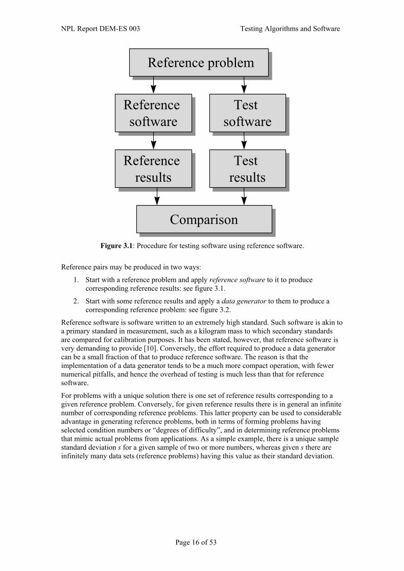
Figure 3.1: Procedure for testing software using reference software.
Reference pairs may be produced in two ways:
1. Start with a reference problem and apply reference software to it to produce corresponding reference results: see figure 3.1.
2. Start with some reference results and apply a data generator to them to produce a corresponding reference problem: see figure 3.2.
Reference software is software written to an extremely high standard. Such software is akin to a primary standard in measurement, such as a kilogram mass to which secondary standards are compared for calibration purposes. It has been stated, however, that reference software is very demanding to provide [10]. Conversely, the effort required to produce a data generator can be a small fraction of that to produce reference software. The reason is that the implementation of a data generator tends to be a much more compact operation, with fewer numerical pitfalls, and hence the overhead of testing is much less than that for reference software.
For problems with a unique solution there is one set of reference results corresponding to a given reference problem. Conversely, for given reference results there is in general an infinite number of corresponding reference problems. This latter property can be used to considerable advantage in generating reference problems, both in terms of forming problems having selected condition numbers or “degrees of difficulty”, and in determining reference problems that mimic actual problems from applications. As a simple example, there is a unique sample standard deviation s for a given sample of two or more numbers, whereas given s there are infinitely many data sets (reference problems) having this value as their standard deviation.
Page 16 of 53

Testing Algorithms and Software NPL Report DEM-ES 003
Reference
results
Reference
results
Reference
data
Reference
problem
Data
generator
Test
software
Test
software Test
results
Test
results
Comparison Comparison
Figure 3.2: Procedure for testing software using a data generator.
To illustrate the design of a data generator, consider the problem specified by the computational aim
“calculate the minimum circumscribed circle for given points in the xy-plane”.
The minimum circumscribed (MC) circle is defined as the circle of minimum radius that circumscribes all the points. Necessary and sufficient conditions for a circle to be the MC circle for given points are as follows:
• There are two points that lie on the circle and form a diameter or there are three points that lie on the circle and form an acute-angled triangle.
• All other points lie on or inside the circle.
These conditions provide a mathematical (and, in this case, geometrical) characterisation of a solution to the problem of calculating the MC circle. We can use the characterisation to design a data generator for this problem in the following way:
1. Start with a circle defined by centre (a, b) and radius R: this is the reference solution.
2. Define three points that lie on the circle and form an acute-angled triangle. For example, the points with co-ordinates
( )αα sin,cos RbRa ++ and
( ))4/3sin(),4/3cos( παπα ±+±+ RbRa will have this property for any choice of angle α.
3. Define all other points to lie on or inside the circle. For example, the points with co-ordinates
( )iiii RbRa θδθδ sin)(,cos)( −+−+
Page 17 of 53

NPL Report DEM-ES 003 Testing Algorithms and Software
will have this property for any choice of angles θi provided 0 ≤ δi ≤ R.
The solution to the MC circle problem for the points generated in this way will be the circle with which we started in step 1. We note that it is easy to generate
• many different reference problems having the same reference solution. This can be done by making different choices for α, δi and θi
• reference problems having particular properties. For example, if we associate the maximum of the deviations δi with “measurement accuracy”, i.e., the “closeness” of the points to the solution circle, we can generate reference problems with different measurement accuracies by assigning the deviations (and their maximum) accordingly.
Most importantly, however, the implementation of a data generator based on the above steps is much more straightforward than implementing reference software for the problem of calculating the MC circle for given points.
There are many computational problems in metrology for which conditions exist to characterise their solution: for such problems it is often possible to design a data generator. A further example of a data generator, in the context of least-squares regression of a model to experimental data, is described in a later chapter.
3.3.3 Specification of quality metrics Quality metrics are used to quantify the performance of the test software for the sequences of reference pairs to which the test software is applied. Furthermore, by specifying the requirements of the user or developer of the test software in terms of these metrics, it is possible to assess objectively whether the test software meets these requirements and is “fit for purpose”. Generally, the metrics measure the departure of the test results returned by the test software from the reference results. The departure may be expressed in terms of the (absolute or relative) difference between the test and reference results, or a performance measure that accounts for factors including the computational precision of the arithmetic used to generate the test and reference results and the conditioning or “degree of difficulty” of the problem defined by a reference pair.
3.3.3.1 Problem condition The condition of a problem is a measure that describes the sensitivity of its exact solution to changes in the problem. If small changes in the problem or its data lead to small changes in the solution, the problem is said to be well-conditioned. Otherwise, if small changes in the data lead to large changes in the solution, the problem is said to be ill-conditioned for the data. Conditioning is an inherent characteristic of the mathematical problem, and is independent of any algorithm or software for solving the problem.
For the very commonly used floating-point arithmetic, the computational precision η is the smallest positive representable number u such that the value 1 + u, computed using the arithmetic, exceeds unity. For the many floating-point processors which today employ IEEE arithmetic, η = 2−52 ≈ 2 × 10⁻¹⁶, corresponding to approximately 16-digit working.
It is unreasonable to expect even software of the highest quality to deliver results for a problem to the full accuracy indicated by the computational precision η. This would only in general be possible for (some) problems that are perfectly conditioned, i.e., problems for which a small change in the data makes a comparably small change in the results. Problems regularly arise in which the ill-conditioning is significant and for which no algorithm, however good, can provide results to the accuracy obtainable for well-conditioned problems.
By using an appropriate performance measure (see below) to quantify the loss of numerical accuracy caused by the test software over and above that which can be explained by the
Page 18 of 53
Testing Algorithms and Software NPL Report DEM-ES 003
problem condition, the type of testing considered here can implicitly identify the use of a poor choice of algorithm or formula from a set of mathematically (but not numerically) equivalent forms. The calculation of the performance measure requires knowledge of the relative condition number κ(x) of the problem specified by values x, defined by
,)(xx
yy
xδδ
κ =
where δx denotes a small perturbation of x and δy the corresponding perturbation of the solution y to the problem, and
∑=
=n
iiv
1
2v
for an n-vector v = (v1, v2, …, vn)T. An analysis of the computational aim specifying the problem is necessary to derive the relative condition number, and such an analysis is often technically demanding. For this reason, it may not always be possible to evaluate the performance measure. However, the performance measure is expected to be more useful for the developer of the test software for whom investigating the numerical properties of the software is important, whereas for users of the software consideration of the (absolute and relative) quality metrics described below is often adequate. Expressions for the relative condition number for some simple problems, including a difference calculation, the calculation of sample standard deviation and the problem of linear least-squares regression, are available [13].
3.3.3.2 Quality metrics Suppose the reference results and test results corresponding to a reference problem defined by values x of the inputs to the test software are expressed as vectors y(ref) and y(test), respectively, of floating-point numbers. Let
.)ref()test( yyy −=∆
Then,
)()( yx ∆= RMSd (1)
is an absolute measure of departure of the test results from the reference results for the reference problem x. Here,
n
RMSv
v =)(
denotes the root-mean-square value of an n-vector v = (v1, v2, …, vn)T. For a scalar-valued result y or when applied to a single component of a vector-valued result, the measure reduces to
.)( )ref()test( yyd −=x (2)
In cases where the components of y are not comparably scaled, some care is required when interpreting the summary measure d(x) defined by (1), and consideration of the component-wise measure (2) is recommended.
The number N(x) of significant figures of agreement between the test results and reference results corresponding to reference data x is calculated from:
If d(x) ≠ 0,
Page 19 of 53

NPL Report DEM-ES 003 Testing Algorithms and Software
.)(
)(1log),(min)()(
10⎭⎬⎫
⎩⎨⎧
⎟⎟⎠
⎞⎜⎜⎝
⎛+=
xyxx
dRMSMN
ref
If d(x) = 0,
).()( xx MN =
Here, M(x) is the number of correct significant figures in the reference results corresponding to x, and is included to account for the fact that, due to the condition of the problem, the reference results may themselves have limited precision. In the same way as for the absolute measures of accuracy described above, N(x) may be applied for the complete vector y or its components.
A performance measure P(x) is calculated, for y(ref) ≠ 0, from
.)(
11log)()(10 ⎟
⎟
⎠
⎞
⎜⎜
⎝
⎛ ∆+=
refP
yy
xx
ηκ
The measure quantifies the performance of the test software and accounts for the following factors:
• the difference between the test and reference results given by ∆y
• the condition of the reference problem defined by x given by the relative condition number κ(x)
• the computational precision η.
The performance measure P(x) indicates, for the reference data set x, the number of significant figures of accuracy lost by the test software over and above the number expected to be lost by an optimally stable algorithm. A value of P(x) close to zero indicates that, for the reference data set x, the test software returns a test result with a relative accuracy that is comparable to that achieved by an optimally stable algorithm. A value of P(x) close to eight, for example, indicates that, for the reference data set x, the test software returns a test result with eight fewer significant figures of accuracy than that returned by an optimally stable algorithm. A related performance measure is used in testing software for evaluating special functions [31].
3.3.3.3 Fitness for purpose If a claim is made about the test software, the claim may be checked for the reference pairs used in the testing. The quality metrics discussed in section 3.3.3.2 are applicable here. For example, if the claim is that the results are accurate to three significant figures, the value of N(x) in section 3.3.3.2 should be three or greater. The claim may originate from the developer of the test software or be a requirement imposed by the user of the software. In either case, testing against the claim can be used as the basis of deciding whether the test software is fit for purpose.
It has been noted in an earlier chapter that the measurement results delivered by software are subject to data effects arising from inexactness in data values (including measurement data, reference constants, calibration information, initial and boundary data, etc.) that define the particular instance of the physical problem required to be solved. Suppose, as in section 3.1, that X and Y denote the input and output quantities, regarded here as random variables, and related by the model Y = f (X), which together define the target computational aim. The inexactness of the input and output quantities is described by the (joint) probability density functions (PDFs) g(X) and g(Y), respectively. The problem addressed in uncertainty evaluation is to determine g(Y) given f and g(X).
Page 20 of 53

Testing Algorithms and Software NPL Report DEM-ES 003
In practice, the computation of the measurement result is undertaken using test software that is an implementation of an algorithm to solve a problem specified by the test computational aim. The output of the test software is denoted by Y(test), also regarded as a random variable, with
).()test()test( XfY =
The inexactness of Y(test) is also described by a PDF, here denoted by g(Y(test)) and determined from f(test) and g(X).
The quality metrics considered in section 3.3.3.2 focus on deciding fitness for purpose using point measures, i.e., by comparing the measurement result y(test) = f(test)(x) delivered by the test software for the reference problem defined by x with the reference result y(ref) = f(x) that would be delivered, for example, by reference software. However, a particular consideration in metrology is to decide fitness for purpose accounting for the inexactness of the input data X. If the difference between the test and reference results is small compared to the possible dispersion of measurement results explained by data effects, then the test software may be regarded as fit for purpose. Such considerations lead us to decide fitness for purpose using statistical measures based on comparing the PDFs g(Y) and g(Y(test)), approximations to which may be obtained using simulation (section 3.5). Such measures allow us to answer questions including, for example:
1. What is the probability of obtaining a solution to the problem specified by the target computational aim that is further from y(ref) than is y(test)?
2. “On average” what is the departure of y(test) from y(ref)?
For simplicity, let us suppose that the output quantity Y is a single scalar quantity. Then, to answer the first question, we wish to evaluate
( ),Pr )ref()test()ref( yyyY −≥−
where “Pr(A)” denotes “probability of A occurring”. This corresponds to finding the area under the curve g(Y) to the left of y(ref) − |y(test) − y(ref)| and to the right of y(ref) + |y(test) − y(ref)| (see figure 3.3), and can therefore be evaluated given knowledge of g(Y). A small probability suggests that y(test), the result delivered by the test software, is not a likely solution to the problem specified by the target computational aim accounting for the inexactness of the input data values.
To answer the second question, we wish to compare the PDFs g(Y ) with g(Y(test)) (see figure 3.4). Particular measures of interest are the differences between the expectation values of the random variables Y and Y(test) and between the variances of those random variables. The difference between the expectation values provides information about any “bias” between the results delivered by the test and reference software. In the example illustrated in figure 3.4we may conclude that (a) there is an appreciable bias between the results, and (b) the dispersion of results delivered by the test software is appreciably greater than that for those delivered by reference software.
Page 21 of 53
NPL Report DEM-ES 003 Testing Algorithms and Software
y(ref)−|y(test)− y(ref)| y(ref) y(ref)+|y(test)− y(ref)|Y
Prob
abili
ty d
ensit
y
Figure 3.3: Measuring the fitness for purpose of test software .
y(test) y(ref)Y
Prob
abili
ty d
ensit
y
Figure 3.4: Probability density functions g(Y), centred on the result y(ref) delivered by reference software, and g(Y(test)), centred on the result y(test) delivered by test software.
Page 22 of 53
Testing Algorithms and Software NPL Report DEM-ES 003
3.4 Complementary checks Examples of tests that do not require the availability of reference pairs are:
• Checking consistency of functions (section 3.4.1)
• Checking continuity of functions (section 3.4.2)
• Checking against tabulated or other values (section 3.4.3)
• Checking solution characterisations (section 3.4.4).
All such checks are to be regarded as complementary to and not alternatives to using reference pairs for algorithm and numerical software testing.
3.4.1 Checking consistency of functions An example of this type of test is the use of a forward followed by an inverse calculation, or vice versa. For example, given test software for sin x and test software for sin−1 x, the values of sin−1sin x can be compared with x for a range of values of x. It is essential to observe that this form of checking alone is insufficient. Two functions could in principle form a near-perfect “inverse pair” but apply to a different mathematical operation.
3.4.2 Checking continuity of functions The algorithms underpinning much mathematical software for special functions such as Bessel functions utilise several mathematical approximations (Chebyshev series, rational functions, etc.), each of which is valid over sub-ranges of the argument(s) of the function. By evaluating the function over suitable ranges of the argument(s), it is possible to gauge the extent to which the returned values are continuous across sub-range boundaries. The presence of discontinuities can have a damaging effect on software that uses these functions as modules, e.g., in adaptive quadrature and optimisation. The documentation accompanying such software may sometimes indicate the sub-range boundaries. Otherwise, they may be inferred from the testing process by graphing the results for a dense set of input-argument values.
3.4.3 Checking against tabulated or other values For certain arguments or ranges of the argument(s) it may be possible to compare the results produced by test software with tabulated values or the results from other software. As an example, functions of a complex variable can be reduced to real functions if the argument is purely real or purely imaginary or through the use of mathematical identities, e.g.,
,sincos xixeix +=
and related formulae. In such cases alternative software may exist which is already well characterised.
3.4.4 Checking solution characterisations In addition to their use as the basis of data generators, solution characterisations can be valuable for checking directly the results returned by test software [1]. For example, we can check whether the circle returned by test software for calculating the minimum circumscribed circle satisfies the (necessary and sufficient) conditions for a solution to this problem (section 3.3.2). The approach requires no knowledge of a reference solution. Instead, we rely on the fact that it is possible to test the properties the solution is supposed to possess using the given characterisation. Such tests constitute post-processing tests of the software and can be applied using simulated test data or data arising in the real world.
Page 23 of 53

NPL Report DEM-ES 003 Testing Algorithms and Software
3.5 Simulation The approaches described in sections 3.3 and 3.4 are focused on testing software using particular reference problems x. It is recommended that the approaches are applied for a range of reference problems typical of those likely to be encountered in practice. This can mean sampling (perhaps uniformly) from the domain of all possible problems that are likely to be encountered, including those close to the boundaries of this domain. In addition, and in order to assess using statistical measures the fitness for purpose of the test software accounting for inexactness in the input quantities X (section 3.3.3.3), it is recommended that the approaches are applied using reference problems sampled from the probability density function g(X) that describes the available knowledge about the inexactness of the input data.
For example, reference and test software for solving, respectively, the problems specified by the target and test computational aims may be combined with simulation in the following manner:
Choose a number M of trials.
1. For r = 1, …, M:
2. Construct the data set xr as a random sample from the PDF g(X).
a. Apply reference software for the target computational aim to the data set xr to obtain reference results yr
(ref).
b. Apply test software for the test computational aim to the data set xr to obtain test results yr
(test).
c. Construct an approximation )(~ Yg to the PDF g(Y) using the set of reference results yr
(ref), r = 1, …, M.
3. Construct an approximation )(~ )test(Yg to the PDF g(Y(test)) using the set of test results yr
(test), r = 1, …, M.
4. Compare g(ref)(Y) with g(test)(Y), for example, in the manner described in section 3.3.3.3.
3.6 Presentation and interpretation of results Having applied the test software to a reference problem to give a test result, the test result is compared with reference results corresponding to the reference problem by computing one or more of the quality metrics described in section 3.3.3. If a sequence of problems is available corresponding to a range of values of a performance parameter (section 3.3.1), the quality metrics may be computed as functions of this parameter. The values of the quality metrics may be presented either in tabular form or as a graph plotted against the performance parameter. It is also convenient to give summary statistics for the computed quality metrics, including their arithmetic means, sample standard deviations, minima and maxima in order to give insight into how the performance of the test software depends on the performance parameter.
A graph of the values of the performance parameter P(x) plotted against the problem condition κ(x) (or some related performance parameter), can provide valuable information about the software. The resulting performance profile can be expressed as a series of points (or the set of straight-line segments joining them). By introducing variability into each data set for each value of the performance parameter, e.g., by using random numbers in a controlled way to simulate observational error, the performance profile will become a swathe of “replicated’’ points, which can be advantageous in the fair comparison of rival algorithms.
Fitness for purpose implies that the test software meets requirements as specified using quality metrics or other appropriate measures (section 3.3.3.3). The user should verify
Page 24 of 53

Testing Algorithms and Software NPL Report DEM-ES 003
whether the reference problem(s) used can be regarded as sufficiently representative of the application in which the software is to be used. It is necessary to decide whether absolute or relative or statistical measures of accuracy are relevant.
The performance measure P(x) indicates the number of figures of accuracy lost by the test software in the computing the test results compared with the reference results (section 3.3.3.2). A large value may indicate the use of an unstable parameterisation of the problem, the use of an unstable algorithm or inappropriate formula, or that the test software is defective. If for graded reference data sets taken in order the corresponding performance measures P(x) have a tendency to increase, it is likely that an unstable parameterisation, formula or numerical method has been employed.
Page 25 of 53
NPL Report DEM-ES 003 Testing Algorithms and Software
4. Discrete Modelling Example: Gaussian Peak Fitting
4.1 Understanding the testing problem The first task is to document what we know about (a) the problem the test software is intended to solve, and (b) how the test software solves that problem.
For test software to solve the problem of fitting a Gaussian peak model to experimental data, we record below (a) the target computational aim (section 4.1.1), (b) the test computational aim (section 4.1.2), and (c) information about how the test software solves the problem specified by the test computational aim (section 4.1.3).
4.1.1 Target computational aim For the example considered here, the following statement may be regarded as sufficient to specify the problem the test software is intended to solve:
“The test software calculates the least-squares best-fit Gaussian peak to data for which the values of the dependent variable are subject to independent and identically distributed random noise.”
Alternatively, the problem may be defined in terms of the inputs to, and outputs from, the software, and an input/output model as follows:
• Inputs: Abscissa values xi, i = 1, …, m, and corresponding ordinate values yi, i = 1, …, m.
• Outputs: Values of the parameters A, x and s in the model
⎟⎟⎠
⎞⎜⎜⎝
⎛ −−= 2
2
2)(exp)(
sxxAxy (1)
for a Gaussian peak, and residual deviations ei, i = 1, …, m, associated with the model, where
).( iii xyye −= (2)
• Input/output model: The outputs are determined from the inputs by solving the following (non-linear) least-squares problem:
( ) ,)(min1
2,, ∑
=
−m
iiisxA xyy
and evaluating the residual deviations (2) associated with the solution model.
4.1.2 Test computational aim We suppose that test software is implemented to solve a problem defined in terms of inputs and outputs as for the target computational aim but with a different an input/output model as follows:
• Input/output model: The outputs are determined from the inputs by solving the following least-squares problem:
( ) ,)(lnlnmin 2,, ∑
∈
−Ii
iisxA xyy
where I = i: yi > 0.
Page 26 of 53
Testing Algorithms and Software NPL Report DEM-ES 003
4.1.3 Implementation of the test software A Gaussian peak model may also be written in the form:
( ) .0,exp)( 22
210 <++= axaxaaxy
The values of the parameters A, x and s in the natural parameterisation (1) of the Gaussian model are then recovered from the values of a0, a1 and a2 using the following relationships:
.21,
2,
4exp
22
1
2
21
0 as
aa
xa
aaA −=−=⎟⎟
⎠
⎞⎜⎜⎝
⎛−=
For reasons of numerical stability, a better representation is the centred form:
( ) ,0,)()(exp)( 22
02010 <−+−+= bxxbxxbbxy (3)
where
,21,
2,
4exp
22
10
2
21
0 bs
bb
xxb
bbA −=−=⎟⎟
⎠
⎞⎜⎜⎝
⎛−= (4)
and x0 is a specified shift in the variable x.
In terms of the parameterisation (3), the test computational aim reduces to the linear least-squares problem:
( )( ) .()(lnmin22
02010∑∈
−+−+−Ii
iii xxbxxbbyb
This is equivalent to finding the least-squares solution to the overdetermined systems of linear equations
,tb =K (5)
where t contains the elements ti = ln yi, i ∈ I, and K is the matrix with rows
( ) .)()(1 200 Iixxxx ii ∈−−
The test software solves the linear least-squares problem (5) using a matrix-factorisation approach [27], uses (4) to obtain values for A, x and s in the Gaussian peak model (1), and (2) to obtain values for the residual deviations ei, i = 1, …, m, associated with the solution model.
4.2 Applying analysis to the testing problem For the problem of fitting a Gaussian peak model to experimental data, we record below some results from mathematical analysis applied to the computational aims (section 4.2.1), and numerical analysis applied to the test software (section 4.2.2).
4.2.1 Mathematical analysis of the computational aims We seek the conditions, i.e., the requirements on the measurement data (xi, yi), i = 1, …, m, for which the problems defined by the target and test computational aims give (a) identical solutions, and (b) comparable solutions. Of course, even if the problems deliver comparable estimates of the values of the parameters for A, x and s, the uncertainties associated with the estimates may be quite different. We do not consider here the conditions under which the problems deliver estimates and associated uncertainties that are comparable.
Page 27 of 53

NPL Report DEM-ES 003 Testing Algorithms and Software
Define
.),(lnln Iixyyf iii ∈−=
Clearly, if the data is such that
,,...,1),( mixyy ii ==
for certain values of A, x and s, i.e., there is no error associated with the measurements of the dependent variable, then the problems will deliver identical solutions, for in this case I = 1, 2, …, m and
,,,1,0 mife ii K===
at the solution.
Now,
( ),)(lnln iii exyy +=
and so by a first order Taylor series expansion
.)(
1)(lnln ii
ii exy
xyy +≈
Therefore,
.)(
1i
ii e
xyf ≈
Only if xi, i = 1, …, m, are such that the values y(xi) are essentially constant can we expect the problems to be approximately equivalent. This is the case, for example, if the measurements are restricted to a tail of the underlying Gaussian peak function. However, in such circumstances, the data will not define the underlying Gaussian peak function very well, and the problem of determining the parameters of this function can be expected to be ill-conditioned.
4.2.2 Numerical analysis of the test software For given values of xi, i = 1, …, m, the matrix K in the overdetermined system of equations (5) and, in particular, the relative condition number κ of the problem defined by those equations, are functions of the value of the shift x0. As an example, let m = 101 and xi be chosen to be uniformly-spaced in the interval from −4 to +4. Table 4.1 lists values (to the nearest integer) of κ corresponding to different choices of the shift x0.
x0 0 1 2 3 4 5 6 7 8 9 10 κ 11 14 20 43 97 198 369 636 1031 1590 2357
Table 4.1: For given shift x0, values (to the nearest integer) of the relative condition κ number of the problem defined by the overdetermined system of equations (5).
As x0 is increased, so the problem defined by the equations (5) becomes increasingly ill-conditioned. Consequently, the numerical performance of any software to solve the problem defined by the equations (5) can be expected to be dependent on the choice of x0. If a matrix-factorisation approach is used to solve the equations (5), as it is stated in section 4.1.3, an upper bound on the number of decimal digits of accuracy that can be expected to be lost by software to solve the equations (5) is log10 κ If an approach based on forming and solving the normal equations was instead used, an upper bound is given by log10 κ2.
Page 28 of 53

Testing Algorithms and Software NPL Report DEM-ES 003
4.3 Applying reference pairs to the testing problem The focus of this example is on applying reference pairs to the testing problem defined in section 4.1. We record below the performance parameters (and their values) used to specify reference pairs (section 4.3.1), the approach to calculating reference pairs (section 4.3.2), and the quality metrics used to compare reference and test results (section 4.3.3).
4.3.1 Specification of reference pairs Performance parameters for the Gaussian peak fitting problem include (i) the peak height A, (ii) the peak location x , (iii) the peak width s, (iv) the data noise σ, (v) the number m of abscissa values xi, (vi) the shift parameter x0 in the Gaussian peak model (7), and (vii) the data width w, i.e., the semi-range of the xi values, given by ½(maxxi − minxi).
Performance parameters (i)−(iii) are used to define the model (1) in the specification of the target computational aim (section 4.1.1), and therefore control the range of solutions returned by the test software. Performance parameter (vi) is a parameter of the algorithm implemented by the test software, and influences the numerical performance of the algorithm (section 4.2.2). The remainder of the performance parameters relate to properties of the input data provided to the test software.
The results described in section 4.4 relate to reference pairs defined by values of the above performance parameters set as follows:
,3,1or0,101,01.00,1,1000,11
0 swxm
xmsxAm
ii ===≤≤=== ∑
=
σ
with xi, i = 1, …, m, uniformly-spaced in the interval from sx 3− from sx 3+ .
4.3.2 Calculation of reference pairs A solution to the problem specified by the target computational aim is characterized by the condition
,T 0e =J
where J is the matrix of partial derivatives
,3,2,1,,...,1),(, ==−=∂∂ jmixyyebe
iiij
i
and both J and e are evaluated at the solution (defined by parameter values b). Based on this condition, a procedure for generating reference data yi, i = 1, …, m, for which the solution to the problem specified by the target computational aim (section 4.1.1) is given a priori takes the following form [3, 13, 26].
Given values for A, x , s, x0, xi: i = 1, …, m:
1. Form values for parameters b from those for A, x and s.
2. Form the model values y(xi), i = 1, …, m.
3. Form the Jacobian matrix J.
4. Form a set of target residual deviations e0,i, i = 1, …, m.
5. Form the null space N for JT.
6. Form the residual vector e = Nu, where u = NTe0.
7. Form the measurement values yi = y(xi) + ei, i = 1, …, m.
Page 29 of 53
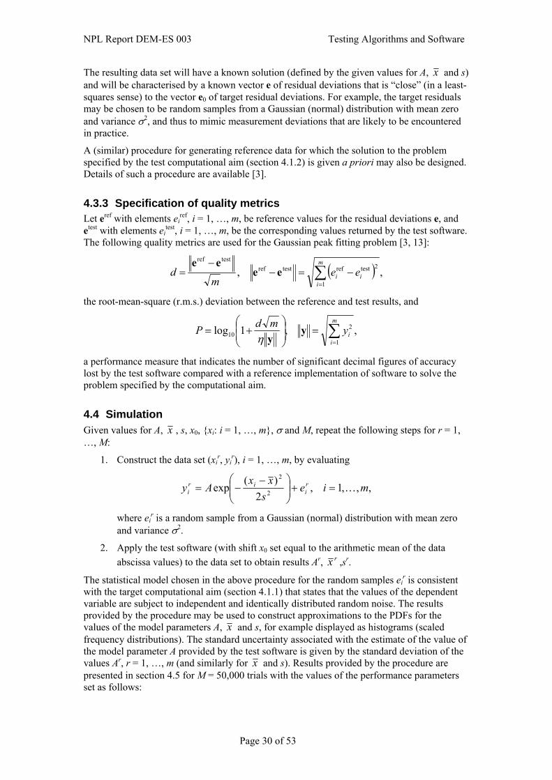
NPL Report DEM-ES 003 Testing Algorithms and Software
The resulting data set will have a known solution (defined by the given values for A, x and s) and will be characterised by a known vector e of residual deviations that is “close” (in a least-squares sense) to the vector e0 of target residual deviations. For example, the target residuals may be chosen to be random samples from a Gaussian (normal) distribution with mean zero and variance σ2, and thus to mimic measurement deviations that are likely to be encountered in practice.
A (similar) procedure for generating reference data for which the solution to the problem specified by the test computational aim (section 4.1.2) is given a priori may also be designed. Details of such a procedure are available [3].
4.3.3 Specification of quality metrics Let eref with elements ei
ref, i = 1, …, m, be reference values for the residual deviations e, and etest with elements ei
test, i = 1, …, m, be the corresponding values returned by the test software. The following quality metrics are used for the Gaussian peak fitting problem [3, 13]:
( ) ,,1
2testreftestreftestref
∑=
−=−−
=m
iii ee
md ee
ee
the root-mean-square (r.m.s.) deviation between the reference and test results, and
,,1log1
210 ∑
=
=⎟⎟⎠
⎞⎜⎜⎝
⎛+=
m
iiymdP y
yη
a performance measure that indicates the number of significant decimal figures of accuracy lost by the test software compared with a reference implementation of software to solve the problem specified by the computational aim.
4.4 Simulation Given values for A, x , s, x0, xi: i = 1, …, m, σ and M, repeat the following steps for r = 1, …, M:
1. Construct the data set (xir, yi
r), i = 1, …, m, by evaluating
,,,1,2
)(exp 2
2
mies
xxAy r
iir
i K=+⎟⎟⎠
⎞⎜⎜⎝
⎛ −−=
where eir is a random sample from a Gaussian (normal) distribution with mean zero
and variance σ2.
2. Apply the test software (with shift x0 set equal to the arithmetic mean of the data abscissa values) to the data set to obtain results Ar, rx ,sr.
The statistical model chosen in the above procedure for the random samples eir is consistent
with the target computational aim (section 4.1.1) that states that the values of the dependent variable are subject to independent and identically distributed random noise. The results provided by the procedure may be used to construct approximations to the PDFs for the values of the model parameters A, x and s, for example displayed as histograms (scaled frequency distributions). The standard uncertainty associated with the estimate of the value of the model parameter A provided by the test software is given by the standard deviation of the values Ar, r = 1, …, m (and similarly for x and s). Results provided by the procedure are presented in section 4.5 for M = 50,000 trials with the values of the performance parameters set as follows:
Page 30 of 53

Testing Algorithms and Software NPL Report DEM-ES 003
,3,1,101,01.0,1,1000,11
0 swxm
xmsxAm
ii ======= ∑
=
σ
with xi, i = 1, …, m, uniformly-spaced in the interval from sx 3− from .3sx +
We would like to compare the standard uncertainties with those that are associated with estimates of the values of the model parameters provided by reference software for solving the problem specified by the target computational aim. This would allow us to investigate whether the quality of the measurement results is unduly affected by the choice of test computational aim and software to solve the problem specified by that computational aim.
If reference software is available, we can use simulation (as above) to provide the standard uncertainties associated with the solution to the problem specified by the target computational aim. Otherwise, analysis of the problem specified by the target computational aim may be used to provide the necessary information (at least approximately). For the problem considered here, the uncertainty (covariance) matrix associated with estimates of the solution to the problem specified by the target computational aim is [5, 19]
( ) ,1T2 −= JJV σ
where J is the matrix of partial derivatives (Jacobian matrix) defined in section 4.3.2. The diagonal elements of this matrix contain the squares of the required standard uncertainties.
4.5 Presentation and interpretation of results Figure 4.1 shows how the values of the quality metrics d and P (section 4.3.3) vary with the performance parameter σ for the case that the shift x0 is set equal to the arithmetic mean of the data abscissa values. The results shown relate to reference data for which the solution to the problem specified by the test computational aim (section 4.1.2) is given a priori. Figure 4.2 shows the same information but for the case that the shift x0 is set equal to zero.
The results indicate that for the reference data sets considered here the test software with x0 equal to the arithmetic mean of the data abscissa values performs almost as well as a reference implementation of software for solving the problem specified by the test computational aim. On the other hand, the test software with x0 equal to zero is losing between five and six significant figures of accuracy compared with reference software for solving this problem. The test software with x0 set equal to zero cannot be regarded as a reference implementation. In both cases there is no strong dependence of the values of the quality metrics d and P on the performance parameter σ.
The results shown in figure 4.1 and figure 4.2, and discussed above, concern numerical software testing of the test software against the test computational aim. In contrast, the results shown in figure 4.3 and figure 4.4 are based on comparing the results returned by the test software with reference results for the problem specified by the target computational aim. The results indicate that the test software, irrespective of the way the shift x0 is set, does not provide accurate solutions to the problem specified by the target computational aim. Because the test software solves the problem specified by the test computational aim to an accuracy that is appreciably greater than that for the problem specified by the target computational aim, we conclude that the results shown in these figures are predominantly a consequence of the difference between the computational aims rather than being attributable to the software implementation. This conclusion applies irrespective of how the shift x0 is set, and we are therefore able, in this example, to deduce useful information about the computational aims from a poor algorithm for solving the problem specified by the test computational aim. The results shown in figure 4.3 and figure 4.4 concern algorithm testing of the test computational aim against the target computational aim.
Figure 4.5 shows approximations to the PDFs for the values of A, x and s constructed using the results returned by the simulation procedure described in section 4.4. Table 4.2 gives, in
Page 31 of 53
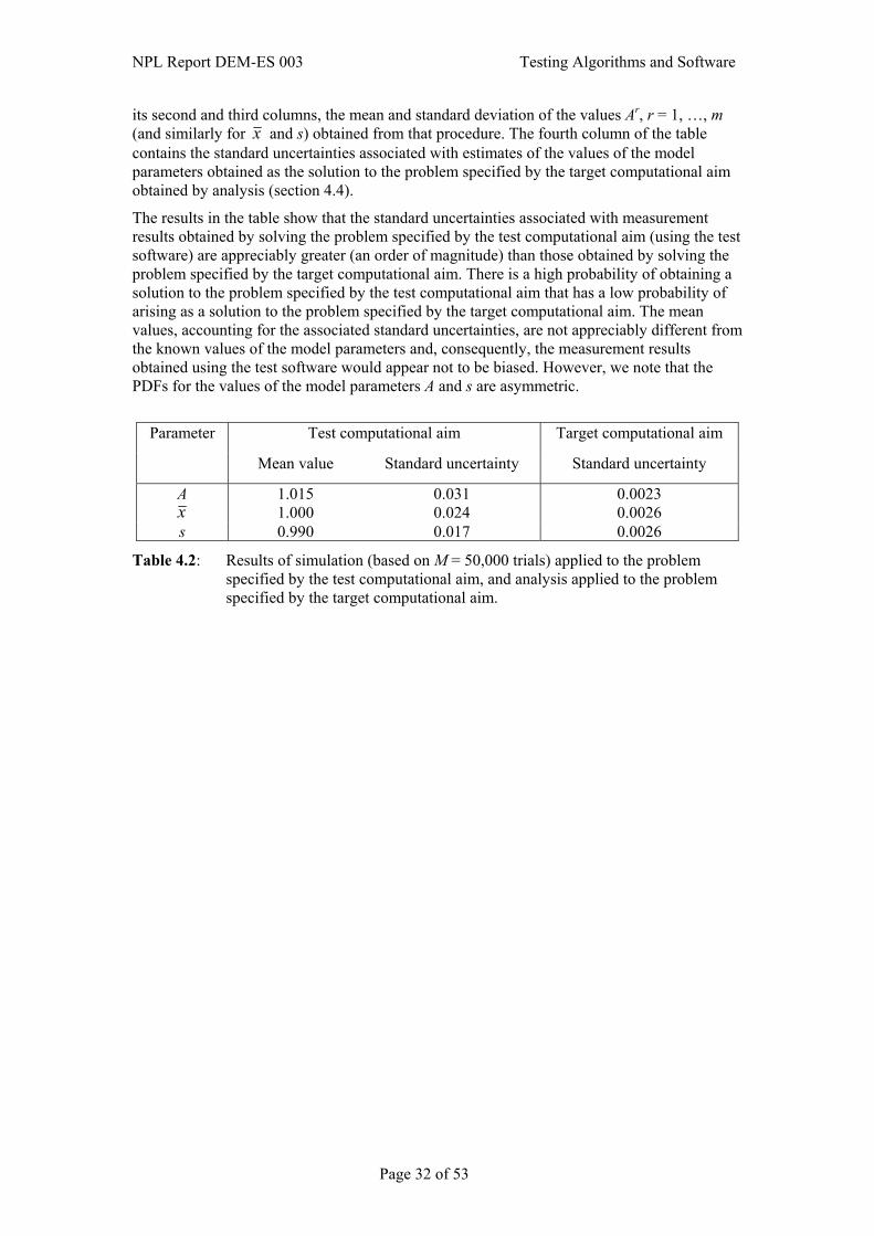
NPL Report DEM-ES 003 Testing Algorithms and Software
its second and third columns, the mean and standard deviation of the values Ar, r = 1, …, m (and similarly for x and s) obtained from that procedure. The fourth column of the table contains the standard uncertainties associated with estimates of the values of the model parameters obtained as the solution to the problem specified by the target computational aim obtained by analysis (section 4.4).
The results in the table show that the standard uncertainties associated with measurement results obtained by solving the problem specified by the test computational aim (using the test software) are appreciably greater (an order of magnitude) than those obtained by solving the problem specified by the target computational aim. There is a high probability of obtaining a solution to the problem specified by the test computational aim that has a low probability of arising as a solution to the problem specified by the target computational aim. The mean values, accounting for the associated standard uncertainties, are not appreciably different from the known values of the model parameters and, consequently, the measurement results obtained using the test software would appear not to be biased. However, we note that the PDFs for the values of the model parameters A and s are asymmetric.
Test computational aim Target computational aim Parameter
Mean value Standard uncertainty Standard uncertainty
A 1.015 0.031 0.0023 x 1.000 0.024 0.0026 s 0.990 0.017 0.0026
Table 4.2: Results of simulation (based on M = 50,000 trials) applied to the problem specified by the test computational aim, and analysis applied to the problem specified by the target computational aim.
Page 32 of 53
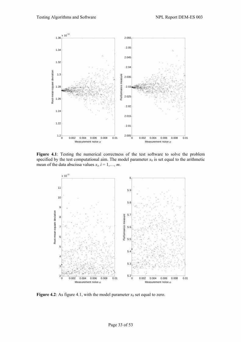
Testing Algorithms and Software NPL Report DEM-ES 003
0 0.002 0.004 0.006 0.008 0.011.2
1.22
1.24
1.26
1.28
1.3
1.32
1.34
1.36x 10⁻¹⁴
Measurement noise σ
Roo
t-mea
n-sq
uare
dev
iatio
n
0 0.002 0.004 0.006 0.008 0.012.005
2.01
2.015
2.02
2.025
2.03
2.035
2.04
2.045
2.05
2.055
Measurement noise σ
Per
form
ance
mea
sure
Figure 4.1: Testing the numerical correctness of the test software to solve the problem specified by the test computational aim. The model parameter x0 is set equal to the arithmetic mean of the data abscissa values xi, i = 1,…, m.
0 0.002 0.004 0.006 0.008 0.012
3
4
5
6
7
8
9
10
11
x 10-11
Measurement noise σ
Roo
t-mea
n-sq
uare
dev
iatio
n
0 0.002 0.004 0.006 0.008 0.015.2
5.3
5.4
5.5
5.6
5.7
5.8
5.9
6
Measurement noise σ
Per
form
ance
mea
sure
Figure 4.2: As figure 4.1, with the model parameter x0 set equal to zero.
Page 33 of 53
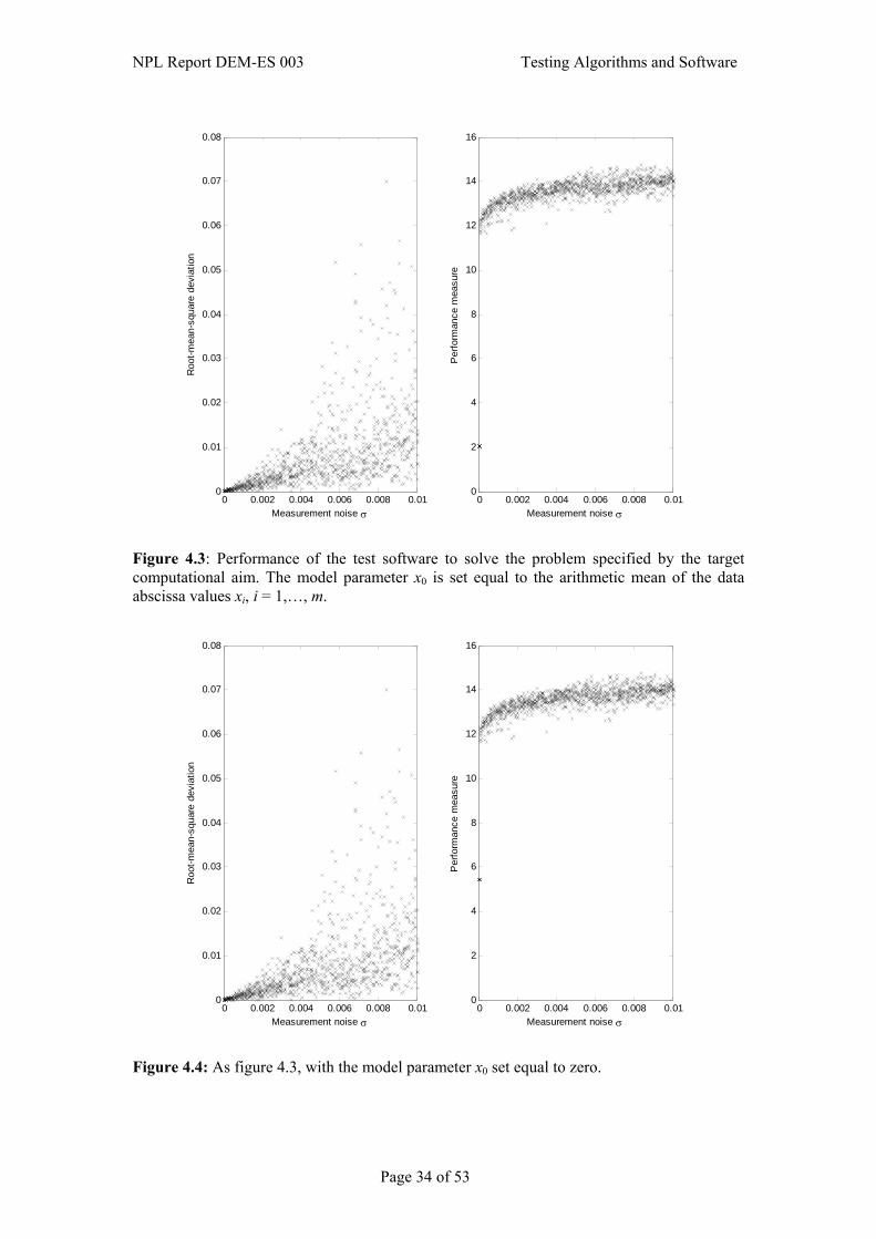
NPL Report DEM-ES 003 Testing Algorithms and Software
0 0.002 0.004 0.006 0.008 0.010
0.01
0.02
0.03
0.04
0.05
0.06
0.07
0.08
Measurement noise σ
Roo
t-mea
n-sq
uare
dev
iatio
n
0 0.002 0.004 0.006 0.008 0.010
2
4
6
8
10
12
14
16
Measurement noise σ
Per
form
ance
mea
sure
Figure 4.3: Performance of the test software to solve the problem specified by the target computational aim. The model parameter x0 is set equal to the arithmetic mean of the data abscissa values xi, i = 1,…, m.
0 0.002 0.004 0.006 0.008 0.010
0.01
0.02
0.03
0.04
0.05
0.06
0.07
0.08
Measurement noise σ
Roo
t-mea
n-sq
uare
dev
iatio
n
0 0.002 0.004 0.006 0.008 0.010
2
4
6
8
10
12
14
16
Measurement noise σ
Per
form
ance
mea
sure
Figure 4.4: As figure 4.3, with the model parameter x0 set equal to zero.
Page 34 of 53
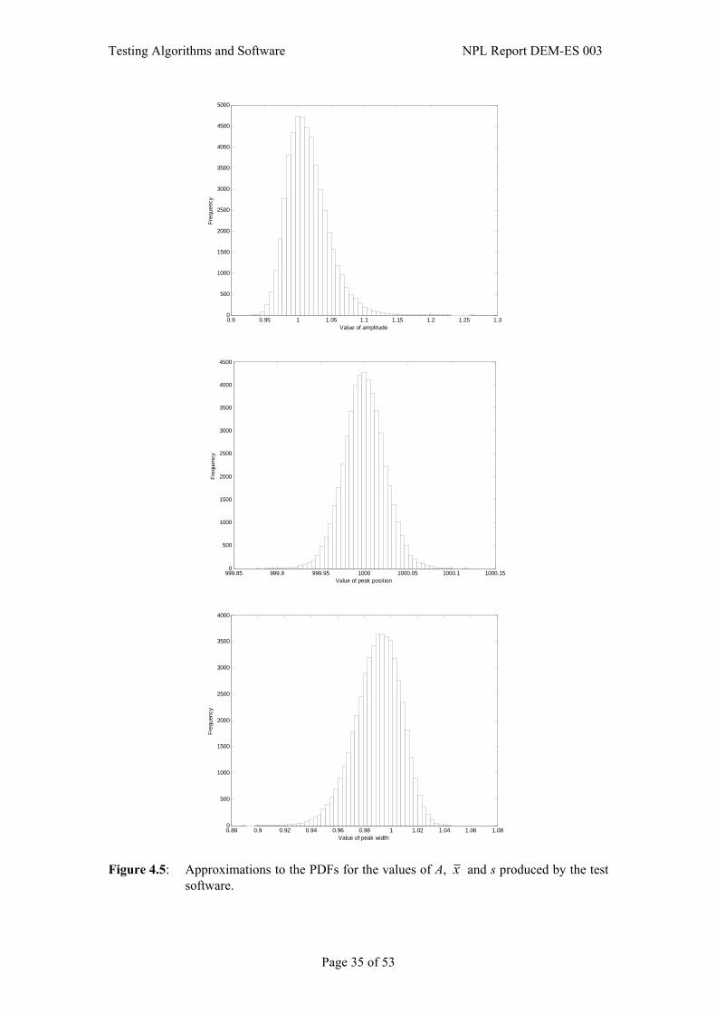
Testing Algorithms and Software NPL Report DEM-ES 003
0.9 0.95 1 1.05 1.1 1.15 1.2 1.25 1.30
500
1000
1500
2000
2500
3000
3500
4000
4500
5000
Value of amplitude
Freq
uenc
y
999.85 999.9 999.95 1000 1000.05 1000.1 1000.150
500
1000
1500
2000
2500
3000
3500
4000
4500
Value of peak position
Freq
uenc
y
0.88 0.9 0.92 0.94 0.96 0.98 1 1.02 1.04 1.06 1.080
500
1000
1500
2000
2500
3000
3500
4000
Value of peak width
Freq
uenc
y
Figure 4.5: Approximations to the PDFs for the values of A, x and s produced by the test
software.
Page 35 of 53

NPL Report DEM-ES 003 Testing Algorithms and Software
5. Continuous Modelling Example: Heat Transfer
5.1 Understanding the testing problem As with any software testing, the first stage in testing continuous modelling software is to define the computational aim. The computational aim of a continuous modelling software package will include some or all of the following:
The (system of) differential equations to be solved
The geometry of the domain
Material properties within the domain
Initial, boundary and loading conditions
Information about the way the geometry is meshed
The first of these points, the specification of the differential equations, must be included. The other four points are less important since most software packages can handle a range of geometries, material properties, and boundary conditions. In some cases it is more straightforward to give a physical description of the computational aim, but the description must still be unambiguous.
The computational aim can be split into two parts: the target computational aim and the test computational aim. For the vast majority of continuous modelling software, the target computational aim is the solution of some set of integral or differential equations, and the test computational aim specifies the method that will be used to generate a numerical approximation to the solution of the equations. The nature of the method is explained more fully in the section on the implementation of the test software, as a thorough understanding of the software can lead to improved test designs.
5.1.1 Target computational aim A physical definition of the target computational aim of the test software could be
“The test software solves the transient heat equation in two dimensions for a prescribed domain, time interval, thermal conductivity, density, specific heat capacity, and set of boundary and initial conditions, giving values of temperature throughout the domain and time interval.”
A full mathematical definition of the same problem could be
“The test software obtains values of T(r, t) by solving
( ) ( )( ) ( )( ) ( )
( ) ( ) ( )( ) ,t,,TT
,tt,,t,T,fT.t,Tt,
tt,,t,T,qTt,T,.Tt,T,ct,T,t p
00
0
0 =Ω∈=
′≤≤Ω∂∈=∇+
′≤≤Ω∈+∇∇=∂∂
rrrrrβr
rrrrr
α
λρ
for specified functions α, β, ρ, cp, λ, q, f, and T0 ,a specified value of t’, and a specified two-dimensional domain Ω”.
The mathematical definition given above is very general but it can be made more relevant to the underlying physical problem by restricting the boundary conditions: not every choice of function for α, β, and f corresponds to a physically meaningful boundary condition. In general, heat transfer boundary conditions model either fixed temperatures, fixed heat fluxes, convective transfer, or radiative transfer. Similarly, realistic assumptions could be made about
Page 36 of 53

Testing Algorithms and Software NPL Report DEM-ES 003
ρ (density), cp (specific heat capacity), and λ (thermal conductivity) as they are physical properties of a material. With this in mind, the computational aim could be written as
“The test software obtains value of T(r, t) by solving
( ) ( ) ( )( ) ( )
( )
( ) ( )
( ) ( ) ( )( )
( ) ( ) ( )( )( ) 0
0
0
0
0
0
0
44
=Ω∈=
′≤≤Ω∂∈−=∂∂
′≤≤Ω∂∈−=∂∂
′≤≤Ω∂∈=∂∂
′≤≤Ω∂∈=
′≤≤Ω∈+∇∇=∂∂
t,,TT
,tt,,t,TTt,nTt,T,
,tt,,t,TTt,hnTt,T,
,tt,,t,qnTt,T,
,tt,,t,TT
,tt,,t,T,qTt,T,.Tt,T,ct,T,t
radambr
convambr
fixqbr
fixtb
p
rr
rrrr
rrrr
rrr
rr
rrrrr
σελ
λ
λ
λρ
for specified functions, λ, ρ, cp, q, Tb, qb, Tamb, h, σ, ε and T0, a specified value of t’, and a specified two-dimensional domain Ω, where ∂Ωfixt, ∂Ωfixq, ∂Ωconv, ∂Ωrad is a partition of the boundary ∂Ω”.
This definition is still not couched in physical terms. For instance, it is not stated that r is position, that T is temperature, or that t is time. However, the expressions used in the definition of the computational aim are all analogous to physical aspects of heat transfer.
5.1.2 Test computational aim The test software used in our examples is finite element software, and the examples use second-order isoparametric elements. The test computational aim is then
“Solve the transient heat equation in two dimensions for a prescribed domain, time interval, thermal conductivity, density, specific heat capacity, and set of boundary and initial conditions, using second-order isoparametric finite elements, to produce temperature values throughout the domain and time interval”
Parameters related to the mesh definition, which have a strong effect on the results, will be defined within each of the tests.
5.1.3 Implementation of the test software Second-order finite elements are either triangles or quadrilaterals which may have curved sides. A discretised version of the differential equations an the boundary conditions is created by mapping the elements in the actual domain to the canonical elements shown in figure 5.1, approximating the temperature by writing
( ) ( )( )( ) ( )( )( )
( )( )( ) ( )( )( )
( )( )( ) ( )( )( )
( )( )( ) ( )( )( )ηξηξξηξ
ξηηξηηξ
ηηξηξηξ
ξηξηξηξηξ
−−++−++−+
−+−+−+−++
+−−++−−+−
+−−+++−−−≈
11141111
21
11141111
21
11121111
41
11121111
41
87
65
43
21
TT
TT
TT
TT,T
Page 37 of 53

NPL Report DEM-ES 003 Testing Algorithms and Software
for quadrilateral elements, or
( ) ( )( ) ( ) ( )( ) ( )ηηξηηξη
ξξξηξηξηξηξ2142214
21142211
654
321
−++−−+−+−−+−−−−≈
TTTTTT,T
for triangular elements, applying this approximation to the heat equation and boundary conditions, and combining all the local approximations in a large matrix of linear equations.
In most cases the temperature is approximated using points that lie within the elements, because certain choices of point provide more accurate approximations for integral calculations, but the user generally requires results to be calculated at the nodal points, so there may be an interpolation stage following the solution of the matrix equations. The approximations above have been written in terms of the nodal points because it is an easier form to write and to understand.
Note that the quadrilateral polynomial’s highest order term is of degree 3. Other finite element formulations exist that preserve continuity of first derivatives at the nodal points, but they are not considered here.
T4
0
η
1
0 ξ1
T1 T2
T3
T5
T6
1
1 -1
-1T1 T2 T3
T4 T5
T6 T7 T8
η
ξ
Figure 5.1: Canonical second-order finite elements.
The most important steps in the software implementation are the formulation of the approximations within the elements and the assembly and solution of the matrix of linear equations. These steps drive the forms of test that are suggested for use with continuous modelling software.
5.2 Applying analysis to the testing problem Applying analysis to the computational aims and implementations of continuous modelling software can indicate forms of test that could be useful. In particular, it may be possible to find analytic solutions to simplified versions of the computational aims, or to exploit features of the software to generate problems with well-understood reference solutions.
5.2.1 Mathematical analysis of the computational aims The test computational aim and the implementation of the software show that the local approximation of the temperature is either a quadratic polynomial or a cubic one, depending on whether the element is a triangle or a quadrilateral. All quadratic functions of x and y obey
Page 38 of 53
Testing Algorithms and Software NPL Report DEM-ES 003
the steady-state heat equation if the material properties are uniform and constant and the x2 and y2 coefficients are of equal magnitude and opposite sign . Hence if a problem is specified such that the boundary conditions are the same quadratic function of position everywhere on the boundary of the domain, and the material properties are constant and uniform, then the test computational aim and the target computational aim will be identical for any shape of domain. This feature can be used to define a set of domain tests.
The most general form for the differential equation used in the target computational aim of the software is
( ) ( )( ) ( )( ) ( ) ,,t,T,qTt,T,.Tt,T,ct,T,t p Ω∈+∇∇=
∂∂ rrrrr λρ
but if the material properties (λ, ρ, and cp) are constant and uniform and there is no internal heat generation (q = 0), the equation can be simplified to
.,Tct
T
pΩ∈∇=
∂∂ r2
ρλ
Hence if a problem can be developed with constant uniform properties and boundary conditions that are independent of the material properties, then any two problems that have the same boundary conditions, the same domain, and the same value of λ/ρcp will have the same solution. This is an example of a property of the computational aim that can be used to define a set of scalable tests.
5.2.2 Numerical analysis of the test software Various numerical techniques and results are available that give an upper bound on the accuracy of finite element methods. In general these techniques are focussed on the differences between a perfectly computed infinite precision numerical solution and the analytic solution (the “discretisation error”), rather than the difference between a real-world finite precision solution and the analytic solution. The techniques usually produce an upper bound on the discretisation error in terms of some property of the mesh.
A set of tests could be defined that took a single example of the target computational aim and solved it using a set of meshes that have known values for the property used in the discretisation error estimate, and the difference between the expected behaviour and the actual behaviour could be examined. This technique is particularly useful for regular meshes within rectilinear geometries, since bounds are generally tightest for such meshes. This technique was discussed as a model validation technique in an SSfM report on continuous model validation [23].
It was mentioned in section 5.1.3 that the two key steps in finite element solution of a problem are element formulation and solution of the matrix of linear equations. Whilst both of these steps will affect the accuracy of the solution to all problems, it is likely that the matrix solution step will be more accurate for problems with a few elements than problems with a large number of elements. It is often straightforward to write down analytic solutions to the test computational aim for problems that only feature a few elements, even for non-linear problems. Hence it can be easy to create sets of reference problems featuring only a small number of elements in order to test element formulation.
5.3 Applying reference pairs to the testing problem The definition of a reference problem for continuous modelling software must contain a definition of the equations, domain, material properties and boundary or loading or initial conditions, as well as the nature of the target results. All of these quantities are required to
Page 39 of 53
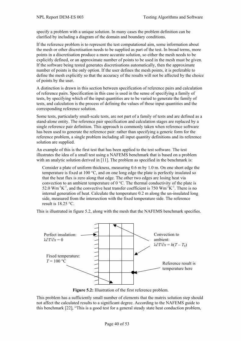
NPL Report DEM-ES 003 Testing Algorithms and Software
specify a problem with a unique solution. In many cases the problem definition can be clarified by including a diagram of the domain and boundary conditions.
If the reference problem is to represent the test computational aim, some information about the mesh or other discretisation needs to be supplied as part of the test. In broad terms, more points in a discretisation produce a more accurate solution, so either the mesh needs to be explicitly defined, or an approximate number of points to be used in the mesh must be given. If the software being tested generates discretisations automatically, then the approximate number of points is the only option. If the user defines the mesh points, it is preferable to define the mesh explicitly so that the accuracy of the results will not be affected by the choice of points by the user.
A distinction is drawn in this section between specification of reference pairs and calculation of reference pairs. Specification in this case is used in the sense of specifying a family of tests, by specifying which of the input quantities are to be varied to generate the family of tests, and calculation is the process of defining the values of those input quantities and the corresponding reference solution.
Some tests, particularly small-scale tests, are not part of a family of tests and are defined as a stand-alone entity. The reference pair specification and calculation stages are replaced by a single reference pair definition. This approach is commonly taken when reference software has been used to generate the reference pair: rather than specifying a generic form for the reference problem, a single problem including all input quantity definitions and its reference solution are supplied.
An example of this is the first test that has been applied to the test software. The test illustrates the idea of a small test using a NAFEMS benchmark that is based on a problem with an analytic solution derived in [11]. The problem as specified in the benchmark is:
Consider a plate of uniform thickness, measuring 0.6 m by 1.0 m. On one short edge the temperature is fixed at 100 °C, and on one long edge the plate is perfectly insulated so that the heat flux is zero along that edge. The other two edges are losing heat via convection to an ambient temperature of 0 °C. The thermal conductivity of the plate is 52.0 Wm-1K-1, and the convective heat transfer coefficient is 750 Wm-2K-1. There is no internal generation of heat. Calculate the temperature 0.2 m along the un-insulated long side, measured from the intersection with the fixed temperature side. The reference result is 18.25 °C.
This is illustrated in figure 5.2, along with the mesh that the NAFEMS benchmark specifies.
Convection to ambient: λ∂T/∂x = h(T – T0)
Fixed temperature: T = 100 °C
Perfect insulation: λ∂T/∂x = 0
Reference result is temperature here
Figure 5.2: Illustration of the first reference problem.
This problem has a sufficiently small number of elements that the matrix solution step should not affect the calculated results to a significant degree. According to the NAFEMS guide to this benchmark [22], “This is a good test for a general steady state heat conduction problem,
Page 40 of 53

Testing Algorithms and Software NPL Report DEM-ES 003
as it specifies a combination of boundary conditions which results in a highly variable temperature field in two dimensions”.
5.3.1 Specification of reference pairs The remaining tests used in this example can have their definitions separated into specification and calculation stages.
The second set of tests is an example of a scalable set of tests. The aim of these tests is to test the ability of the software to solve problems with a wide range of values for the input parameters. The reference problem is an axisymmetric transient problem:
Consider a uniform cylinder of unit radius and unit length. Initially one end of the cylinder is at 20 and the rest of the cylinder is at 0. All sides of the cylinder are perfectly insulated throughout. The mesh to be used is an evenly-spaced array of 10 quadratic elements in the radial direction and 10 quadratic elements in the axial direction, giving a total of 341 nodes. Note that units are not specified as the problem is independent of the choice of units.
If the thermal conductivity is λ, the density is ρ, and the specific heat capacity is cp, find the temperature at the point r = 0, z = 1, at times ti = 0.01i, i = 1, 2, …, 200. The reference results are given by
( ) ( )[ ]⎟⎟
⎠
⎞
⎜⎜
⎝
⎛−−+= ∑
∞
=1
2exp12131
m
m tmtT πα
where α = λ/(ρcp) is the thermal diffusivity. Note that the problem requires initial conditions to be specified because it is a transient model. The problem is illustrated in figure 5.3. The set of tests is generated by varying the individual values of λ, ρ, and cp, whilst holding the ratio λ/(ρcp) fixed. The properties λ, ρ, and cp are being used as performance parameters to parameterise the space of admissible inputs to the test software.
This problem is related to a laser flash heating model that simulates a method used to determine thermal diffusivity experimentally.
Radius = 1
Initial temperature 20
Length = 1
r = 0
r = 1
z = 0 z = 1
Tinit= 20 Tinit= 0 Solution of interest
(a) (b)Figure 5.3: Illustration of the second reference problem.
Page 41 of 53

NPL Report DEM-ES 003 Testing Algorithms and Software
The third set of tests is based on a simple test expressed in a generic mathematical form. The problem is to solve
( ) ( ) ( ) ,y,x,ayaxaxyayxay,xT
,,T
Ω∂∈=++++−=
Ω∈=∇
r
r
543222
1
2 0
for Ω a two-dimensional domain and the ai a set of constants. This specification leads to a family of tests generated by varying Ω, so initially no domain geometry is specified explicitly. The domain lies within the square –0.05 ≤ x, y ≤ 1.05 and consists of 100 elements. The method used for creating the mesh is outlined in the next section. The required results are the values of T at all the points used to calculate the solution, and the reference results are given by
( ) ( ) ,,ayaxayxayxay,xT *iiiiiiiii Ω∈++++−= x5432
221
where Ω* is the set of points that make up the discrete approximation to the domain used in the calculations, not including points that lie on the boundary.
5.3.2 Calculation of reference pairs The second set of tests as specified in the previous section requires calculation of three parameters (λ, ρ, and cp) subject to a constraint (λ/(ρcp) held fixed). The parameter values used in this case were based on initial values
,.c,.,. p322 1008108210011 ×=×=×= −ρλ
giving α ≈ 0.45, a value that is likely to create a well-conditioned problem. Initially λ and α were both held fixed and ρ and cp were varied by factors of 10: ρ was varied between 2.8×10⁻¹⁰ and 2.8×10¹⁰, and hence cp was varied between 8.0×10⁻¹¹ and 8.0×10⁹. Then λ, ρ, and cp were all varied with α held fixed, such that λ varied between 1.01×10⁻¹⁰ and 1.01×10¹⁰, ρ varied between 2.8×10⁻⁶ and 2.8×10⁵, and cp varied between 8.0×10⁻⁵ and 8.0×10⁴ such that the modulus of difference between the exponents of ρ and cp was less than or equal to 1 at all times. A full list of all parameter sets used in the tests can be found in an earlier report [27].
The final set of tests were defined by creating a mesh of 100 second order elements (341 nodes, 121 corner nodes and 220 mid-side nodes) that covered the whole of the square 0 ≤ x, y ≤ 1 and then allowing the nodes to move by different amounts to perturb the mesh. A total of eleven meshes, including the initial regular mesh, were used. The procedure for creating the meshes was:
1. For the ith mesh, set ri = 0.0025 (i – 1), i = 1, 2, …11.
2. Generate the unperturbed corner nodes cj = (xj, yj), j = 1, 2, …, 121 such that they define a uniform 10 by 10 mesh on the unit square.
3. Generate 121 random numbers sj, j = 1, 2, …, 121, from a uniformly distributed random variable on [0, 2π].
4. Generate the ith perturbed corner nodes from (cj)i = (xj + ri cos sj, yj + ri sin sj) and round to five decimal places.
5. Create mid-side nodes half-way along the straight lines connecting cj to cj-1, cj+1, cj-11, and cj+11.
This procedure produces elements with straight sides, rather than elements that require quadratic expressions to describe them accurately. This choice was made so that the element shape could not get too far away from a square (the ideal shape for a quadrilateral finite element). Since the solution to the problem varies quadratically, the second-order elements described in section 5.1.3 are still necessary.
Page 42 of 53
Testing Algorithms and Software NPL Report DEM-ES 003
This mesh generation procedure will lead to an increasingly distorted set of meshes. It is expected that the more distorted the mesh is, the worse will be the results. The maximum and minimum internal angle of all the elements is a reasonable measure of mesh distortion: an ideal mesh has all angles at 90°, and a mesh is generally regarded as acceptable if all its internal angles lie between 45° and 135°. The distribution of internal angles has been calculated for each mesh, and will be discussed further in section 5.4.
For each mesh, six sets of random values of the ak, k =1, 2, …, 5 were chosen by sampling a uniformly distributed random variable on [1,10], and rounding to two decimal places, and each set of values were used with each mesh. All boundary conditions and reference results were truncated to eight decimal places because the software ignores all figures after the eighth. The random values used were:
Test number a1 a2 a3 a4 a5
1 2.04 1.79 2.98 5.54 6.34 2 3.28 8.7 8.29 5.84 8.53 3 1.45 6.96 9.39 9.55 4.68 4 5.61 5.78 7.31 4.53 3.4 5 3.84 3.57 8.15 1.14 3.12 6 5.95 6.06 3.14 6.85 4.47
Table 5.1: Parameters used to define the reference solutions.
All of these values give rise to results between 0 and 40.
The performance parameters in this set of tests are the coefficients ai, and the radius rj used to perturb the nodal positions.
5.3.3 Specification of quality metrics The choice of quality metrics for continuous models is the same as that for discrete models. It should be noted that almost all continuous models produce a large number of results, so the quality metrics that can be applied to vectors of results are usually the most useful.
Under some circumstances, it can be worth using different quality metrics for different sets of the results. In particular, if the model results are close to zero in one region but not another, it may be helpful to apply an absolute metric where the results are small and a relative metric elsewhere.
Condition numbers, as discussed in section 3.3.3.1, can be difficult to obtain for continuous models, because the implicit nature of most continuous models makes obtaining sensitivity coefficients difficult. Condition of the problem has not been considered explicitly for these problems, but all choices of parameters have been restricted to produce “reasonable” values of the results. For instance, the reference results for all the tests all lie between 0 and 100, so there should be little problem with comparative scaling of results in different regions of the domain.
The reference results in all the tests are O(10), and so the quality metrics used for these examples is, for Tref the reference results and Ttest the test results
( ) ( ) ,t,Tt,TM
M
iii∑
=
−1
2reftest
1 xx
where M is the number of nodes of interest and the summation could potentially be extended to average over time as well.
Page 43 of 53

NPL Report DEM-ES 003 Testing Algorithms and Software
The performance measure
( )( )
( ) ( ) ( ) ( )
( ) ( )⎪⎩
⎪⎨
⎧
=−
>−⎪⎭
⎪⎬⎫
⎪⎩
⎪⎨⎧
⎥⎥⎦
⎤
⎢⎢⎣
⎡
−+
=
,t,Tt,T,
,t,Tt,T,t,Tt,T
t,T,
t,N08
01log8min
testref
testreftestref
ref10
xx
xxxx
xx
is also used, where 8 is chosen because the reference results are known to be accurate to 8 figures.
5.4 Complementary checks It is possible to take the discrete results produced by the software, use them to construct an approximation to the second derivatives of T, and check that this approximation obeys the differential equation. This is a consistency check as described in section 3.3.1. However, for non-rectangular meshes this becomes quite tricky. Hence the check has only been carried out for the first mesh used in the third set of tests as this is a two-dimensional rectangular mesh.
On average, the calculated values of the differential lay between 2.7×10T2∇ -3 and 1.2×10⁻³. These values were obtained without attempting to reconstruct the detailed quadratic approximations used in the model. Instead a simple-minded approximation was constructed using the nodal values. Given the approximation used, results were about as good as could be expected.
The transient tests could have their conservation of energy checked to test the solution characterisation. Since the test results were independent of the input parameters (see section 5.6), this was only done for a single test. Values were found to be constant to seven significant figures, which is a good result.
5.5 Simulation Simulation is often avoided for continuous modelling problems, because the necessary repeated runs of the model can be too computationally expensive to justify. However, some software tools now offer automated running and processing of multiple parameterised jobs in order to explore the “design space” of a model, which can be used as a tool for carrying out sensitivity analyses as described in section 3.5. A simulation exercise on a thermal model is being carried out as part of a different SSfM project, and will be reported in the forthcoming SSfM Good Practice Guide to continuous modelling.
The aim of the simulations described in section 3.5 is similar to the aims of the scalable tests described above: to explore the full ranges of the likely input values. Scalable tests aim for coverage of the full range rather than generation of statistical information, but the aims are still similar.
5.6 Presentation and interpretation of results As was mentioned in section 5.3, it is common for continuous models to produce results at a large number of points. Generally the accuracy of the results is likely to vary as a function of position. Hence it is often useful to present the quality metric values as a graph or surface plot. Where possible this has been done in the examples.
As was mentioned in section 5.1.3, results are often calculated at internal integration points and then extrapolated to nodes. Outputting results at the integration points and checking their accuracy can give an indication of the accuracy of the extrapolation algorithm is. This has not been done for any of the tests described here, because the extrapolation algorithm will be exact for the solutions to the only tests where reference results at domain points are available (the domain tests).
Page 44 of 53
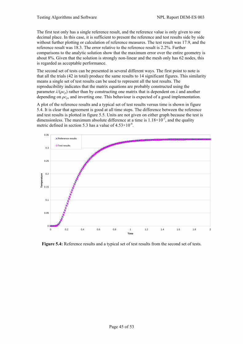
Testing Algorithms and Software NPL Report DEM-ES 003
The first test only has a single reference result, and the reference value is only given to one decimal place. In this case, it is sufficient to present the reference and test results side by side without further plotting or calculation of reference measures. The test result was 17.9, and the reference result was 18.3. The error relative to the reference result is 2.2%. Further comparisons to the analytic solution show that the maximum error over the entire geometry is about 8%. Given that the solution is strongly non-linear and the mesh only has 62 nodes, this is regarded as acceptable performance.
The second set of tests can be presented in several different ways. The first point to note is that all the trials (42 in total) produce the same results to 14 significant figures. This similarity means a single set of test results can be used to represent all the test results. The reproducibility indicates that the matrix equations are probably constructed using the parameter λ/(ρcp) rather than by constructing one matrix that is dependent on λ and another depending on ρcp, and inverting one. This behaviour is expected of a good implementation.
A plot of the reference results and a typical set of test results versus time is shown in figure 5.4. It is clear that agreement is good at all time steps. The difference between the reference and test results is plotted in figure 5.5. Units are not given on either graph because the test is dimensionless. The maximum absolute difference at a time is 1.18×10⁻³, and the quality metric defined in section 5.3 has a value of 4.53×10⁻⁴.
0
0.05
0.1
0.15
0.2
0.25
0.3
0.35
0 0.2 0.4 0.6 0.8 1 1.2 1.4 1.6 1.8 2
Time
Tem
pera
ture
Reference results
Test results
Figure 5.4: Reference results and a typical set of test results from the second set of tests.
Page 45 of 53
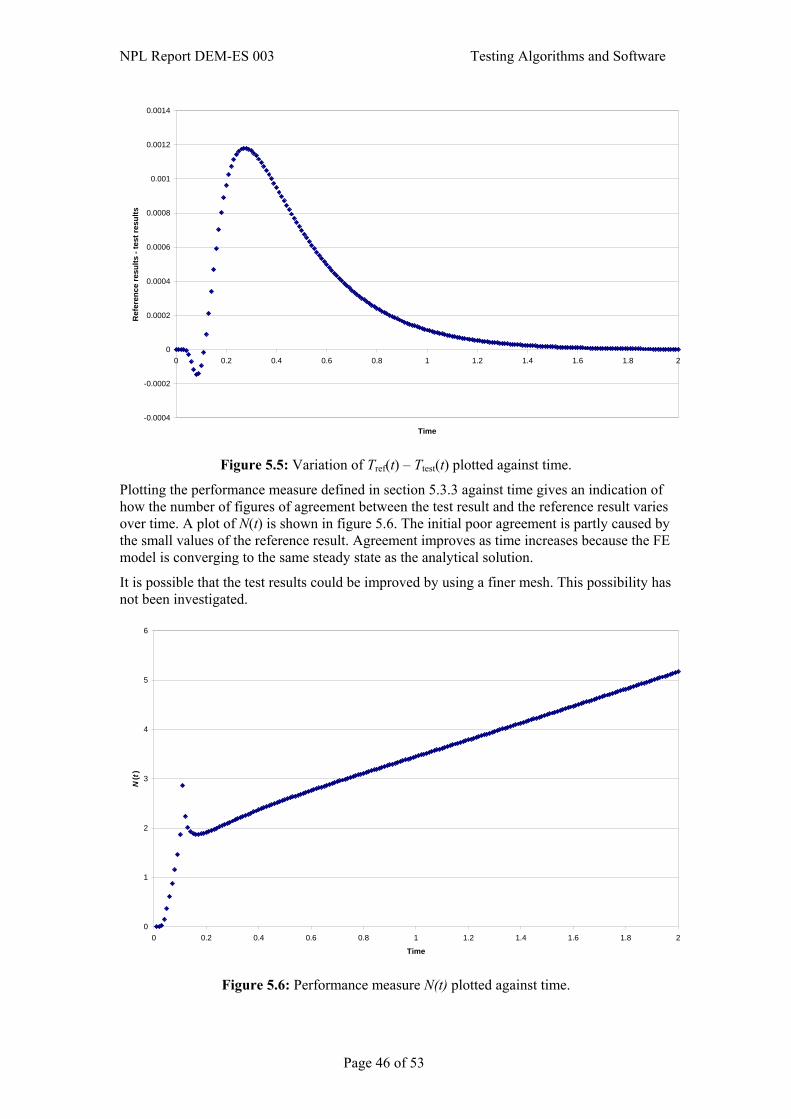
NPL Report DEM-ES 003 Testing Algorithms and Software
-0.0004
-0.0002
0
0.0002
0.0004
0.0006
0.0008
0.001
0.0012
0.0014
0 0.2 0.4 0.6 0.8 1 1.2 1.4 1.6 1.8 2
Time
Ref
eren
ce re
sults
- te
st re
sults
Figure 5.5: Variation of Tref(t) – Ttest(t) plotted against time.
Plotting the performance measure defined in section 5.3.3 against time gives an indication of how the number of figures of agreement between the test result and the reference result varies over time. A plot of N(t) is shown in figure 5.6. The initial poor agreement is partly caused by the small values of the reference result. Agreement improves as time increases because the FE model is converging to the same steady state as the analytical solution.
It is possible that the test results could be improved by using a finer mesh. This possibility has not been investigated.
0
1
2
3
4
5
6
0 0.2 0.4 0.6 0.8 1 1.2 1.4 1.6 1.8 2
Time
N( t
)
Figure 5.6: Performance measure N(t) plotted against time.
Page 46 of 53

Testing Algorithms and Software NPL Report DEM-ES 003
The third set of tests generated six sets of results for eleven different meshes. As was mentioned in section 5.3.2, the quality of the results is likely to depend on the internal angles of the elements in the mesh. The angles for all elements in all meshes were calculated, 400 angles altogether, and the statistics summarising the results are shown in table 5.2. All angles are given in degrees. Note that the range and the standard deviation increase with mesh number, indicating that the mesh is becoming less uniform. Also note that the maximum and minimum angles in meshes 10 and 11 are beyond the recommended values of 135° and 45°.
Mesh number
Average angle
Standard deviation
Maximum angle
Minimum angle
Range
(max – min)
1 90.0 0.00 90.0 90.0 0.0 2 89.9 2.03 94.9 85.1 9.7 3 90.2 4.17 99.3 79.9 19.4 4 90.2 6.05 105.0 75.4 29.6 5 89.8 7.62 110.0 70.0 40.0 6 89.3 10.53 111.6 63.5 48.1 7 89.4 12.60 120.4 59.4 60.9 8 89.9 14.18 126.1 57.0 69.1 9 89.5 17.10 132.6 47.0 85.6
10 90.4 17.48 140.7 40.4 100.4 11 88.2 20.59 142.6 31.6 111.0
Table 5.2: Statistics describing the range of internal angles of the elements within each mesh.
There are several useful ways of looking at the test results. A key point to note is that because the boundary conditions were specified by temperature values at the nodes on the boundary, the accuracy of the test results on the boundary is a measure of the accuracy of the interpolation algorithms and will not be affected by any of the other steps in the calculation. Hence looking at the error in the results at the nodes on the boundary can give an indication of the accuracy of the interpolation algorithms.
As an illustration, compare the first, sixth, and eleventh meshes. RMS absolute differences between the reference and test results averaged over the full, internal, and boundary node sets are shown for each test in table 5.3.
Page 47 of 53
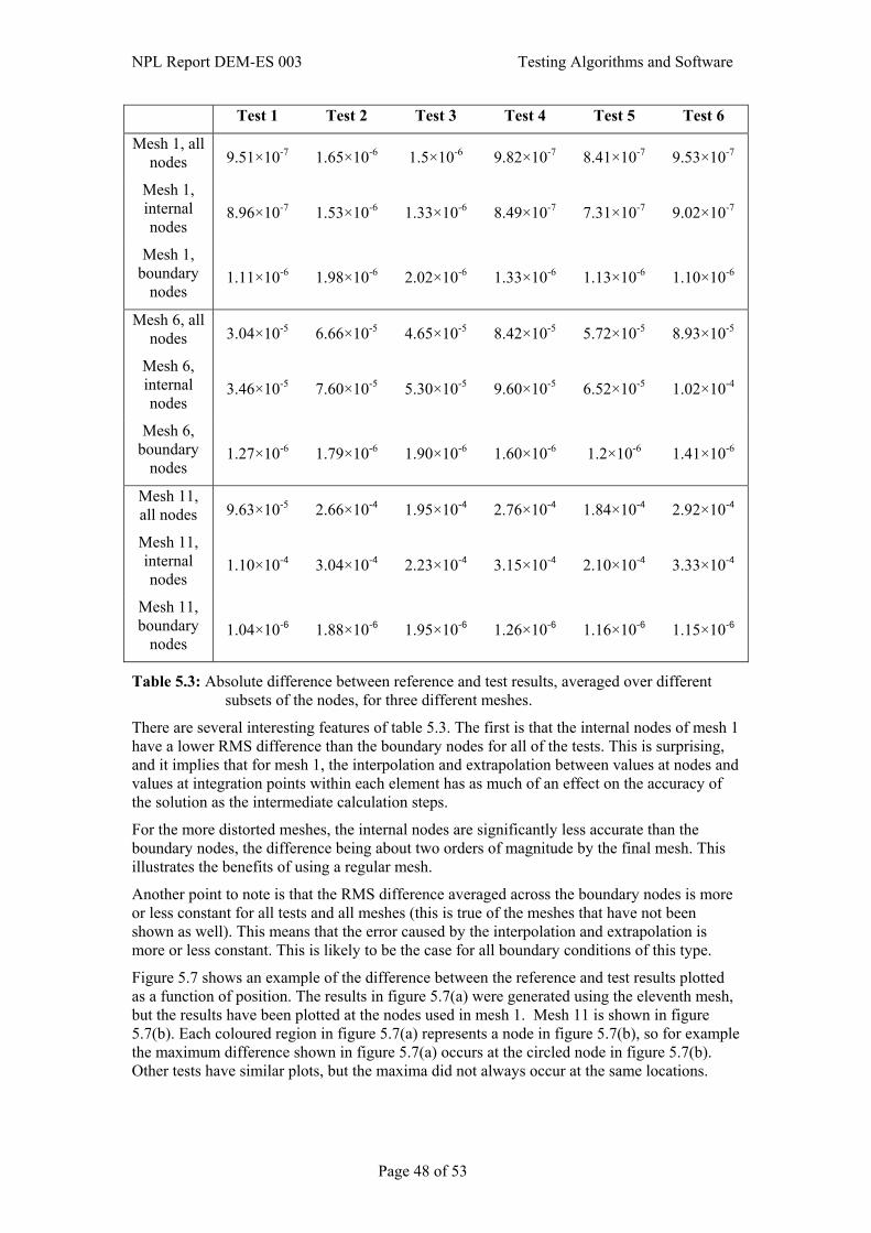
NPL Report DEM-ES 003 Testing Algorithms and Software
Test 1 Test 2 Test 3 Test 4 Test 5 Test 6
Mesh 1, all nodes 9.51×10⁻⁷ 1.65×10⁻⁶ 1.5×10⁻⁶ 9.82×10⁻⁷ 8.41×10⁻⁷ 9.53×10⁻⁷
Mesh 1, internal nodes
8.96×10⁻⁷ 1.53×10⁻⁶ 1.33×10⁻⁶ 8.49×10⁻⁷ 7.31×10⁻⁷ 9.02×10⁻⁷
Mesh 1, boundary
nodes 1.11×10⁻⁶ 1.98×10⁻⁶ 2.02×10⁻⁶ 1.33×10⁻⁶ 1.13×10⁻⁶ 1.10×10⁻⁶
Mesh 6, all nodes 3.04×10⁻⁵ 6.66×10⁻⁵ 4.65×10⁻⁵ 8.42×10⁻⁵ 5.72×10⁻⁵ 8.93×10⁻⁵
Mesh 6, internal nodes
3.46×10⁻⁵ 7.60×10⁻⁵ 5.30×10⁻⁵ 9.60×10⁻⁵ 6.52×10⁻⁵ 1.02×10⁻⁴
Mesh 6, boundary
nodes 1.27×10⁻⁶ 1.79×10⁻⁶ 1.90×10⁻⁶ 1.60×10⁻⁶ 1.2×10⁻⁶ 1.41×10⁻⁶
Mesh 11, all nodes 9.63×10⁻⁵ 2.66×10⁻⁴ 1.95×10⁻⁴ 2.76×10⁻⁴ 1.84×10⁻⁴ 2.92×10⁻⁴
Mesh 11, internal nodes
1.10×10⁻⁴ 3.04×10⁻⁴ 2.23×10⁻⁴ 3.15×10⁻⁴ 2.10×10⁻⁴ 3.33×10⁻⁴
Mesh 11, boundary
nodes 1.04×10⁻⁶ 1.88×10⁻⁶ 1.95×10⁻⁶ 1.26×10⁻⁶ 1.16×10⁻⁶ 1.15×10⁻⁶
Table 5.3: Absolute difference between reference and test results, averaged over different subsets of the nodes, for three different meshes.
There are several interesting features of table 5.3. The first is that the internal nodes of mesh 1 have a lower RMS difference than the boundary nodes for all of the tests. This is surprising, and it implies that for mesh 1, the interpolation and extrapolation between values at nodes and values at integration points within each element has as much of an effect on the accuracy of the solution as the intermediate calculation steps.
For the more distorted meshes, the internal nodes are significantly less accurate than the boundary nodes, the difference being about two orders of magnitude by the final mesh. This illustrates the benefits of using a regular mesh.
Another point to note is that the RMS difference averaged across the boundary nodes is more or less constant for all tests and all meshes (this is true of the meshes that have not been shown as well). This means that the error caused by the interpolation and extrapolation is more or less constant. This is likely to be the case for all boundary conditions of this type.
Figure 5.7 shows an example of the difference between the reference and test results plotted as a function of position. The results in figure 5.7(a) were generated using the eleventh mesh, but the results have been plotted at the nodes used in mesh 1. Mesh 11 is shown in figure 5.7(b). Each coloured region in figure 5.7(a) represents a node in figure 5.7(b), so for example the maximum difference shown in figure 5.7(a) occurs at the circled node in figure 5.7(b). Other tests have similar plots, but the maxima did not always occur at the same locations.
Page 48 of 53
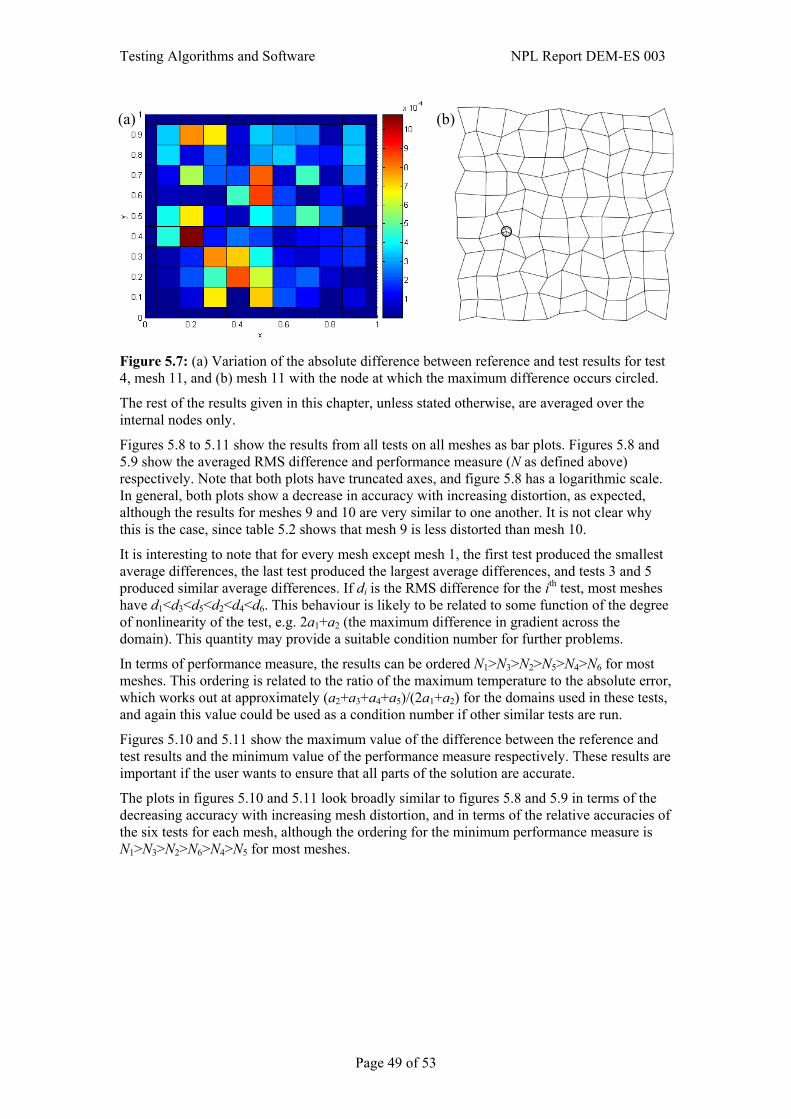
Testing Algorithms and Software NPL Report DEM-ES 003
(a) (b)
Figure 5.7: (a) Variation of the absolute difference between reference and test results for test 4, mesh 11, and (b) mesh 11 with the node at which the maximum difference occurs circled.
The rest of the results given in this chapter, unless stated otherwise, are averaged over the internal nodes only.
Figures 5.8 to 5.11 show the results from all tests on all meshes as bar plots. Figures 5.8 and 5.9 show the averaged RMS difference and performance measure (N as defined above) respectively. Note that both plots have truncated axes, and figure 5.8 has a logarithmic scale. In general, both plots show a decrease in accuracy with increasing distortion, as expected, although the results for meshes 9 and 10 are very similar to one another. It is not clear why this is the case, since table 5.2 shows that mesh 9 is less distorted than mesh 10.
It is interesting to note that for every mesh except mesh 1, the first test produced the smallest average differences, the last test produced the largest average differences, and tests 3 and 5 produced similar average differences. If di is the RMS difference for the ith test, most meshes have d1<d3<d5<d2<d4<d6. This behaviour is likely to be related to some function of the degree of nonlinearity of the test, e.g. 2a1+a2 (the maximum difference in gradient across the domain). This quantity may provide a suitable condition number for further problems.
In terms of performance measure, the results can be ordered N1>N3>N2>N5>N4>N6 for most meshes. This ordering is related to the ratio of the maximum temperature to the absolute error, which works out at approximately (a2+a3+a4+a5)/(2a1+a2) for the domains used in these tests, and again this value could be used as a condition number if other similar tests are run.
Figures 5.10 and 5.11 show the maximum value of the difference between the reference and test results and the minimum value of the performance measure respectively. These results are important if the user wants to ensure that all parts of the solution are accurate.
The plots in figures 5.10 and 5.11 look broadly similar to figures 5.8 and 5.9 in terms of the decreasing accuracy with increasing mesh distortion, and in terms of the relative accuracies of the six tests for each mesh, although the ordering for the minimum performance measure is N1>N3>N2>N6>N4>N5 for most meshes.
Page 49 of 53
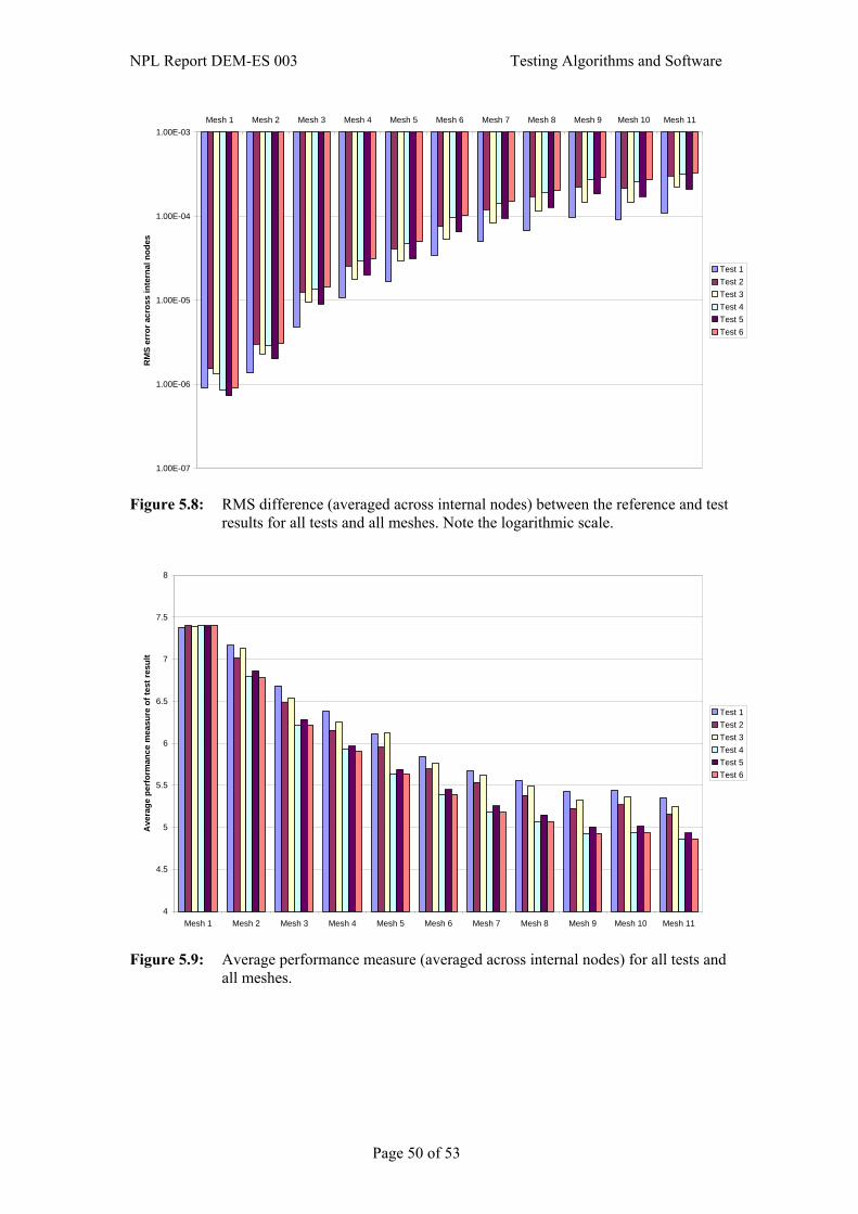
NPL Report DEM-ES 003 Testing Algorithms and Software
1.00E-07
1.00E-06
1.00E-05
1.00E-04
1.00E-03Mesh 1 Mesh 2 Mesh 3 Mesh 4 Mesh 5 Mesh 6 Mesh 7 Mesh 8 Mesh 9 Mesh 10 Mesh 11
RM
S er
ror a
cros
s in
tern
al n
odes
Test 1Test 2Test 3Test 4Test 5Test 6
Figure 5.8: RMS difference (averaged across internal nodes) between the reference and test results for all tests and all meshes. Note the logarithmic scale.
4
4.5
5
5.5
6
6.5
7
7.5
8
Mesh 1 Mesh 2 Mesh 3 Mesh 4 Mesh 5 Mesh 6 Mesh 7 Mesh 8 Mesh 9 Mesh 10 Mesh 11
Ave
rage
per
form
ance
mea
sure
of t
est r
esul
t
Test 1Test 2Test 3Test 4Test 5Test 6
Figure 5.9: Average performance measure (averaged across internal nodes) for all tests and all meshes.
Page 50 of 53

Testing Algorithms and Software NPL Report DEM-ES 003
1.00E-06
1.00E-05
1.00E-04
1.00E-03
1.00E-02Mesh 1 Mesh 2 Mesh 3 Mesh 4 Mesh 5 Mesh 6 Mesh 7 Mesh 8 Mesh 9 Mesh 10 Mesh 11
Max
imum
abs
olut
e er
ror a
cros
s al
l res
ults
Test 1Test 2Test 3Test 4Test 5Test 6
Figure 5.10: Maximum difference between the test results and the reference results. Note the logarithmic scale.
3
3.5
4
4.5
5
5.5
6
6.5
7
Mesh 1 Mesh 2 Mesh 3 Mesh 4 Mesh 5 Mesh 6 Mesh 7 Mesh 8 Mesh 9 Mesh 10 Mesh 11
Min
imum
per
form
ance
mea
sure
of t
est r
esul
t
Test 1Test 2Test 3Test 4Test 5Test 6
Figure 5.11: Minimum value of the performance metric.
Page 51 of 53

NPL Report DEM-ES 003 Testing Algorithms and Software
6. References 1. Anthony, G.T. and M.G. Cox. The design and validation of software for dimensional
metrology. NPL Report DITC 50/84, National Physical Laboratory, 1984.
2. Barker, R.M., P.M. Harris, and G.I. Parkin. Development and Testing of Spreadsheet Applications. Software Support for Metrology Best Practice Guide No. 7, NPL, July 2000. http://www.npl.co.uk/ssfm/download/documents/ssfmbpg7.pdf
3. Barker, R.M., M.G. Cox, P.M. Harris, and I.M. Smith. Testing Algorithms in Standards and METROS. NPL Report CMSC 18/03, NPL, April 2003. http://www.npl.co.uk/ssfm/download/documents/cmsc18_03.pdf
4. Barker, R.M. Guide To EUROMETROS: a manual for users, contributors and testers. Software Support for Metrology Good Practice Guide No. 5, NPL, March 2004. http://www.npl.co.uk/ssfm/download/documents/ssfmgpg5.pdf
5. Barker, R.M., M.G. Cox, A.B. Forbes, and P.M. Harris. Discrete Modelling and Experimental Data Analysis. Software Support for Metrology Best Practice Guide No. 4, NPL, April 2004. www.npl.co.uk/ssfm/download/documents/ssfmbpg4.pdf
6. Barrett, J. and M.P. Dainton. Testing the intrinsic functions of MathCAD. NPL Report CMSC 05/00, September 2000.
7. Barrett, J. and M.P. Dainton. Testing the intrinsic functions of S-PLUS. NPL Report CMSC 06/00, September 2000.
8. Beckett, R.E., M.G. Cox, M.P. Dainton, P.M. Harris, E.G. Johnson, and G.I. Parkin. Testing Methods of Java Libraries. NPL Report CMSC 35/04, NPL, January 2004.
9. Butler, B., M. Cox, A. Forbes, S. Hannaby, and P. Harris. A methodology for testing classes of approximation and optimisation software, in Quality of numerical software: assessment and enhancement. 1996. Oxford: Chapman and Hall.
10. Butler, B.P., M.G. Cox, S.L.R. Ellison, and W.A. Hardcastle, eds. Statistics Software Qualification: Reference Data Sets. Royal Society of Chemistry. 1996: Cambridge.
11. Carslaw, H.S. and J.C. Jaeger, Conduction of Heat in Solids. 1959: Oxford University Press.
12. Clements, T., L. Emmet, P. Froome, and S. Guerra. Test and Measurement Software. Software Support for Metrology Best Practice Guide No. 12, NPL, October 2002. http://www.npl.co.uk/ssfm/download/documents/ssfmbpg12.pdf
13. Cook, H.R., M.G. Cox, M.P. Dainton, and P.M. Harris. A methodology for testing spreadsheets and other packages used in metrology. Report to the National Measurement System Policy Unit, Department of Trade and Industry, from the UK Software Support for Metrology Programme. NPL Report CISE 25/99, NPL, September 1999. http://www.npl.co.uk/ssfm/download/documents/cise25_99.pdf
14. Cook, H.R., M.G. Cox, M.P. Dainton, and P.M. Harris. Testing spreadsheets and other packages used in metrology: A case study. Report to the National Measurement System Policy Unit, Department of Trade and Industry, from the UK Software Support for Metrology Programme. NPL Report CISE 26/99, NPL, September 1999. http://www.npl.co.uk/ssfm/download/documents/cise26_99.pdf
15. Cook, H.R., M.G. Cox, M.P. Dainton, and P.M. Harris. Testing spreadsheets and other packages used in metrology: Testing the intrinsic functions of Excel. Report to the National Measurement System Policy Unit, Department of Trade and Industry, from the UK Software Support for Metrology Programme. NPL Report CISE 27/99, NPL, September 1999. www.npl.co.uk/ssfm/download/docuements/cise27_99.pdf
Page 52 of 53

Testing Algorithms and Software NPL Report DEM-ES 003
16. Cox, M.G. and P.M. Harris, The design and use of reference data sets for testing scientific software. Analytica Chimica Acta, 1999(380): p. 339-351.
17. Cox, M.G., M.P. Dainton, and P.M. Harris. Testing functions for the calculation of standard deviation. NPL Report CMSC 07/00, October 2000.
18. Cox, M.G., M.P. Dainton, and P.M. Harris. Testing functions for linear regression. NPL Report CMSC 08/00, October 2000.
19. Cox, M.G. and P.M. Harris. Uncertainty Evaluation. Software Support for Metrology Best Practice Guide No. 6, NPL, January 2004. http://www.npl.co.uk/ssfm/download/documents/ssfmbpg6.pdf
20. Cox, M.G. and P.M. Harris. Numerical analysis for algorithm design in metrology. Software Support for Metrology Best Practice Guide No. 11, NPL, April 2004. http://www.npl.co.uk/ssfm/download/documents/ssfmbpg11.pdf
21. Cox, M.G., P.M. Harris, E.G. Johnson, P.D. Kenward, and G.I. Parkin. Testing the numerical correctness of software. NPL Report CMSC 34/04, January 2004.
22. Davies, G.A.O., R.T. Fenner, and R.T. Lewis, eds. Background to Benchmarks. 1993, NAFEMS: Glasgow.
23. Esward, T., G. Lord, and L. Wright. Model Validation in Continuous Modelling. CMSC 29/03, NPL, September 2003.
24. Esward, T.J., E.G. Johnson, and L. Wright. Testing Continuous Modelling Software. NPL Report CMSC 41/04, NPL, March 2004.
25. Esward, T.J., K. Lees, D. Sayers, and L. Wright. Testing Continuous Modelling Software: Three Case Studies. NPL Report CMSC 42/04, NPL, June 2004.
26. Forbes, A.B., P.M. Harris, and R.K. Leach. The comparison of algorithms for the assessment of Type A1 surface texture reference artefacts. NPL Report CMSC 33/03, NPL, 2003.
27. Golub, G.H. and C.F. Van Loan, Matrix Computations. third edition ed. 1996, Baltimore: John Hopkins University press.
28. Harris, P.M. and I.M. Smith. Testing algorithms for free-knot spline approximation. NPL Report CMSC 48/04, NPL, March 2004.
29. Higham, N.J. Testing linear algebra software, in Quality of Numerical Software: Assessment and Enhancement. 1996. Oxford: Chapman and Hall.
30. Higham, N.J., Accuracy and Stability of Numerical Algorithms. Second edition ed. 2002: SIAM. xxx+680 pp.
31. Van Snyder, W. Testing functions of one or two arguments, in Quality of Numerical Software: Assessment and Enhancement. 1996. Oxford: Chapman and Hall.
32. Wichmann, B.A., R.M. Barker, and G.I. Parkin. Validation of Software in Measurement Systems. Software Support for Metrology Best Practice Guide No. 1, NPL, March 2004. http://www.npl.co.uk/ssfm/download/documents/ssfmbpg1.pdf
Page 53 of 53