tes characterization for carbon cycle science ppt overview factors that affect co 2 source and sink...

Characterization of Tropospheric Emission Spectrometer (TES) CO2for carbon cycle science

Susan Kulawik, Kevin Bowman, Dylan Jones, Ray Nassar, John Worden, F.W. Irion, Annmarie Eldering, and the TES team

Kevin Bowman – ASSFTS 14

Copyright YEAR California Institute of Technology. Government sponsorship acknowledged.

Talk overview

Factors that affect CO2 source and sink estimates

TES CO2 results and characterization

OSSE to estimate TES CO2 impact on source and sink estimates

Conclusions


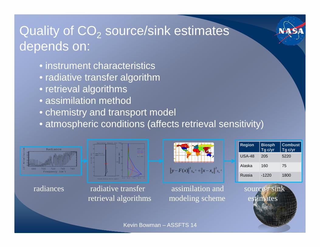
Quality of CO2 source/sink estimates depends on:

Radiance

680 700 720 740 760

Frequency (cm-1)

456789

10

-6 W/cm

2/sr/cm

-1

-1

3

-0.2 0.0 0.2 0.4 0.6

0

10

20

30

40

50

Altitude (km)

100

10

DOFS 1.0

908 hPa511 hPa133 hPa10 hPa0.1 hPa

Retrieval Result for CO2

Volume Mixing Ratio [ppmv]

0

5

10

15

20

25

30

35

Altitude [km] Result

A priori

1000

100

10

Pressure [mb]

1122

)( −− −+− am SaS xxxFy

radiances radiative transfer assimilation and source / sinkretrieval algorithms modeling scheme estimates

• instrument characteristics• radiative transfer algorithm• retrieval algorithms• assimilation method• chemistry and transport model• atmospheric conditions (affects retrieval sensitivity)

Region BiosphTg c/yr

CombustTg c/yr

USA-48 205 5220

Alaska 160 75

Russia -1220 1800


Instrument characteristics- AIRS, IASI, GOSAT, and TES instruments at mid-infrared (700 cm-1):

Native resolution

S/N @native

S/N @ 0.5 cm-1

AIRS 0.5 cm-1 ~525 ~525*

IASI 0.5 cm-1 ~225 ~225**

GOSAT 0.2 cm-1 >300*** >475

TES 0.1 cm-1 ~80 ~200****

* http://airs.jpl.nasa.gov/technology/specifications/ with 0.35K @ 250K; 9 footprint ave** Crevoisier et al., 2009 0.22K error at 700 cm-1*** http://www.jaxa.jp/press/2009/02/20090209_ibuki_e.html, infrared band average**** Shephard et al., 2008 table 2, with 0.3K @250K at AIRS resolution


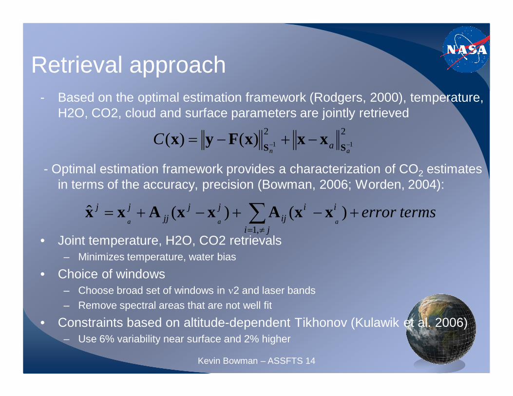
Retrieval approach- Based on the optimal estimation framework (Rodgers, 2000), temperature,

H2O, CO2, cloud and surface parameters are jointly retrieved

- Optimal estimation framework provides a characterization of CO2 estimates in terms of the accuracy, precision (Bowman, 2006; Worden, 2004):

• Joint temperature, H2O, CO2 retrievals– Minimizes temperature, water bias

• Choice of windows– Choose broad set of windows in ν2 and laser bands– Remove spectral areas that are not well fit

• Constraints based on altitude-dependent Tikhonov (Kulawik et al. 2006)– Use 6% variability near surface and 2% higher

2211)()(−−

−+−=an

aCSS

xxxFyx

termserrorji

iiij

jjjj

jj

aaa +−+−+= ∑

≠= ,1

)()(ˆ xxAxxAxx


Radiance

680 700 720 740 760

Frequency (cm-1)

456789

10

-6 W/cm

2/sr/cm

-1

970 975 980 985 990

Frequency (cm-1)

5.86.06.26.46.66.8

10

-6 W/cm

2/sr/cm

-1

1070 1080 1090 1100 1110

Frequency (cm-1)

3.5

4.0

4.5

5.0

10

-6 W/cm

2/sr/cm

-1

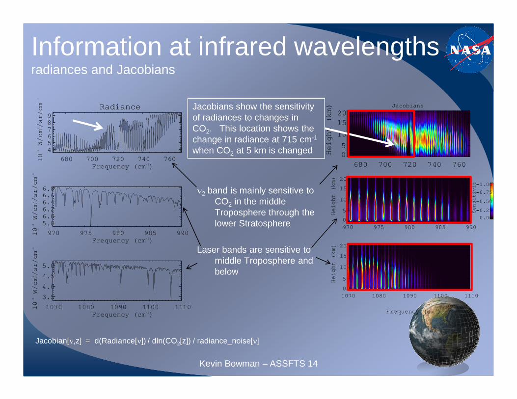
Information at infrared wavelengthsradiances and Jacobians

680 700 720 740 760

0

5

10

15

20

Height (km) Jacobians

970 975 980 985 990

0

5

10

15

20

Height (km)

1070 1080 1090 1100 1110

0

5

10

15

20

Height (km)

Jacobians show the sensitivity of radiances to changes in CO2. This location shows the change in radiance at 715 cm-1

when CO2 at 5 km is changed

10

15

20

0.00

0.25

0.50

0.75

1.00

Sensitivity

----

ν2 band is mainly sensitive to CO2 in the middle Troposphere through the lower Stratosphere

Laser bands are sensitive to middle Troposphere and below

Jacobian[ν,z] = d(Radiance[ν]) / dln(CO2[z]) / radiance_noise[ν]

1070 1080 1090 1100 1110

Frequency (cm-1)


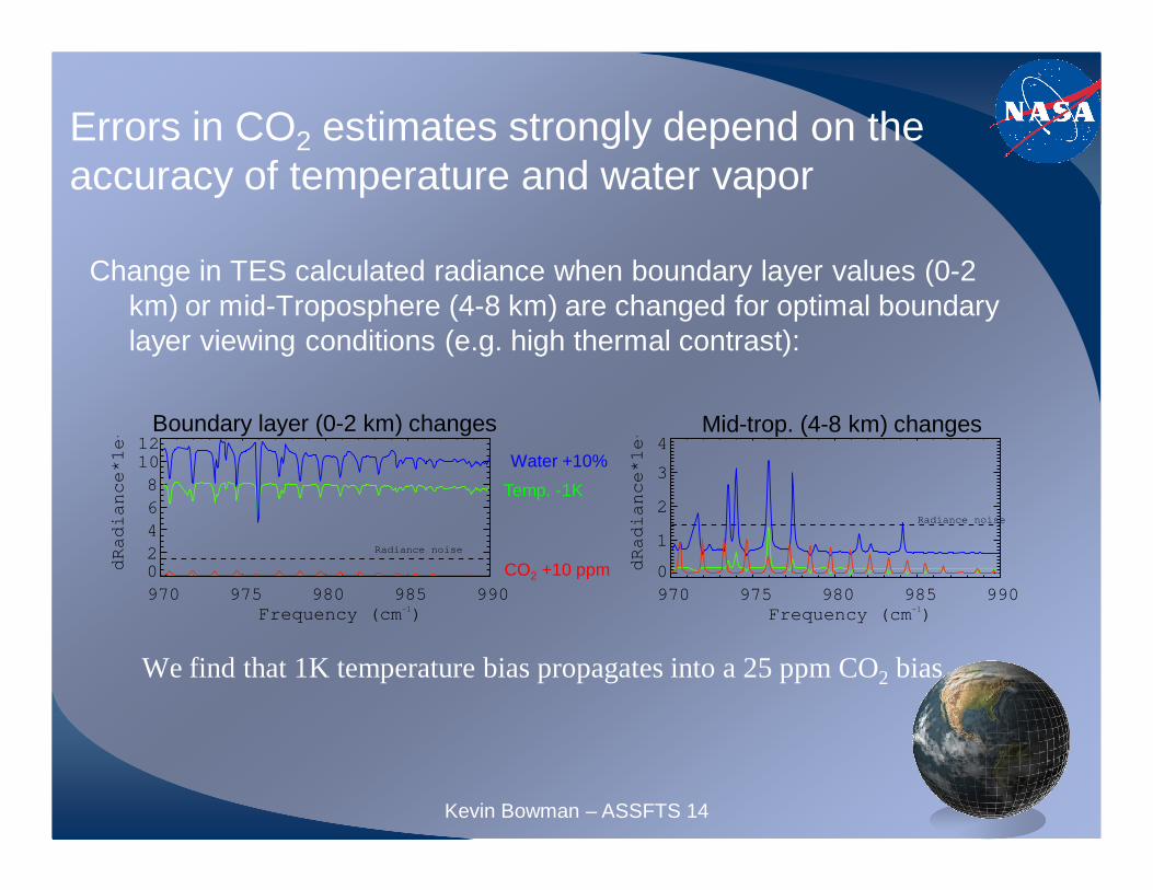
Change in TES calculated radiance when boundary layer values (0-2 km) or mid-Troposphere (4-8 km) are changed for optimal boundary layer viewing conditions (e.g. high thermal contrast):

We find that 1K temperature bias propagates into a 25 ppm CO2 bias

Errors in CO2 estimates strongly depend on the accuracy of temperature and water vapor

970 975 980 985 990

Frequency (cm-1)

0

1

2

3

4

dRadiance*1e-8

Radiance noise

970 975 980 985 990

Frequency (cm-1)

02

4

6

8

1012

dRadiance*1e-8

Radiance noise

Water +10%

Temp. -1K

CO2 +10 ppm

Boundary layer (0-2 km) changes Mid-trop. (4-8 km) changes


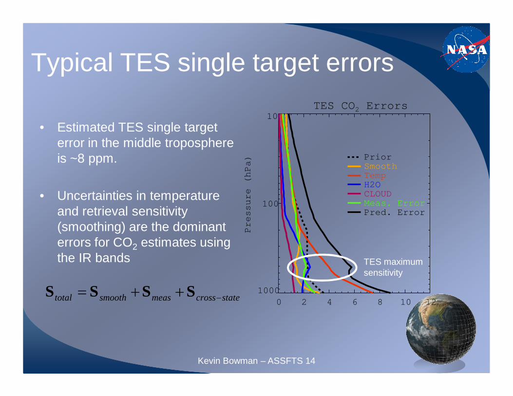
TES CO2 Errors

0 2 4 6 8 10 12

1000

100

10

Pressure (hPa) Prior

SmoothTempH2OCLOUDMeas. ErrorPred. Error

Typical TES single target errors

• Estimated TES single target error in the middle troposphere is ~8 ppm.

• Uncertainties in temperature and retrieval sensitivity (smoothing) are the dominant errors for CO2 estimates using the IR bands TES maximum

sensitivity

statecrossmeassmoothtotal −++= SSSS


Averaging targets

• Averaging more targets (over a larger spatial area) decreases error vs. Mauna Loa

• Progression agrees with 1/sqrt(N) reduction in error for averages

S. Kulawik – March, 2009

CO2 Errors vs. spatial averaging

50 100 150 200

Number of targets

0.0

0.5

1.0

1.5

2.0

Error (ppm)

Error vs. Mauna Loa1/sqrt(n) progression

Tropospheric Emission Spectrometer CO2Observed yearly and seasonal variations are consistent within situ datau

Monthly averages of ~200 targetsMonthly mean error is 0.9 ppm with 5.6 ppm biasBias close to estimated spectroscopic error of ~4 ppm (Devi, 2003)Greatest sensitivity in middle Troposphere (500 mb)Validated for low O.D. cloud, ocean, 40S to 40N

TES CO2 at 511 hPa, 15-30N

2006 2007 2008 2009

Year

365

370

375

380

385

390

395

CO2 VMR (ppm)

TES monthly TES monthly aveave

CONTRAIL aircraft dataCONTRAIL aircraft data Mauna LoaMauna Loa

prior

Highly correlated with Mauna Loa CO2

370 375 380 385 390

TES

370

375

380

385

390

Mauna Loa

corr 0.94

slope 1.02bias -5.6 ppm


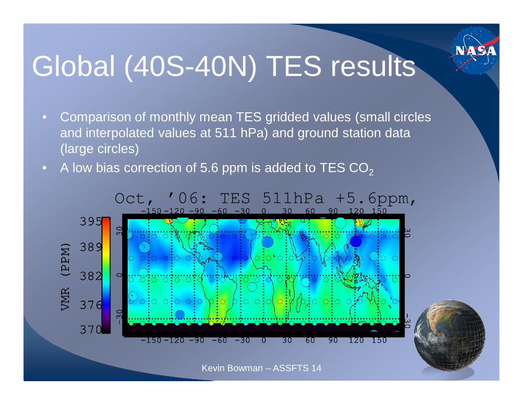
Global (40S-40N) TES results

• Comparison of monthly mean TES gridded values (small circles and interpolated values at 511 hPa) and ground station data (large circles)

• A low bias correction of 5.6 ppm is added to TES CO2


-150 -120 -90 -60 -30 0 30 60 90 120 150

-150 -120 -90 -60 -30 0 30 60 90 120 150

-30

030

-30

030

Oct, ’06: TES 511hPa +5.6ppm, Flasks

370

376

382

389

395

VMR (PPM)

-150 -120 -90 -60 -30 0 30 60 90 120 150

-150 -120 -90 -60 -30 0 30 60 90 120 150

-30

030

-30

030

370

376

382

389

395

VMR (PPM)

-150 -120 -90 -60 -30 0 30 60 90 120 150

-150 -120 -90 -60 -30 0 30 60 90 120 150

-30

030

-30

030

370

376

382

389

395

VMR (PPM)

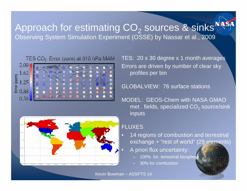
Approach for estimating CO2 sources & sinksObserving System Simulation Experiment (OSSE) by Nassar et al., 2009

TES: 20 x 30 degree x 1 month averages Errors are driven by number of clear sky

profiles per bin

GLOBALVIEW: 76 surface stations

MODEL: GEOS-Chem with NASA GMAO met . fields, specialized CO2 source/sink inputs

FLUXES• 14 regions of combustion and terrestrial

exchange + “rest of world” (29 elements)• A priori flux uncertainty:

– 100% for terrestrial biosphere

– 30% for combustion

Err

or (

ppm

)


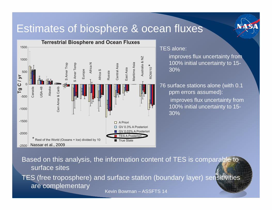
Estimates of biosphere & ocean fluxes

TES alone:improves flux uncertainty from 100% initial uncertainty to 15-30%

76 surface stations alone (with 0.1 ppm errors assumed): improves flux uncertainty from 100% initial uncertainty to 15-30%

Based on this analysis, the information content of TES is comparable to surface sites

TES (free troposphere) and surface station (boundary layer) sensitivities are complementary

Nassar et al., 2009


Conclusions

TES observed yearly and seasonal variations are consistent with in situ data

TES CO2 with error characterization can be used to improve estimates of CO2sources and sinks

Next steps

Using real TES data for source and sink estimates

Examine the use of other sensors for measuring CO2 profiles to improve source and sink estimates

Validation versus aircraft data over land in progress


AcknowledgementsWork at JPL was carried out under contract to NASA with funds from ROSES 2007. Work by

Nassar et al. funded by Natural Sciences and Engineering Research Council (NSERC) of Canada. We acknowledge use of GLOBALVIEW-CO2 and Mauna Loa from NOAA-ESRL and CONTRAIL data from World Data Centre for Greenhouse Gases (WDCGG).

Thanks to H. Worden for S/N calculation help

ReferencesMatsueda, H., H. Y. Inoue, and M. Ishii (2002), Aircraft observation of carbon dioxide at 8-13 km altitude over the western Pacific from 1993 to 1999. Tellus, 54B(1), 1- 21, doi: 10.1034/j.1600-0889.2002.00304.x

Nassar et al, R., D.B.A. Jones, S.S. Kulawik, J.M. Chen. (2009), Use of surface and space-based CO2

observations for inverse modeling of CO2 sources and sinks. (Poster) 2nd North American Carbon Program All-Investigators Meeting, 2009 February 17-20, San Diego, CA.

Palmer, P. I., D. J. Jacob, et al. (2003). "Inverting for emissions of carbon monoxide from Asia using aircraft observations over the western Pacific." Journal of Geophysical Research-Atmospheres 108(D21).

Rodgers, C. (2000). Inverse Methods for Atmospheric Sounding: Theory and Practice. Singapore, World Scientific Publishing Co.

Shephard, M. W., H. M. Worden, et al. (2008). "Tropospheric Emission Spectrometer nadir spectral radiance comparisons." J. Geophys. Res. 113.

U.S. Department of Commerce | National Oceanic and Atmospheric Administration Earth System Research Laboratory | Global Monitoring Division http://www.esrl.noaa.gov/gmd/dv/site/SMO.html

Backup

S. Kulawik – March, 2009

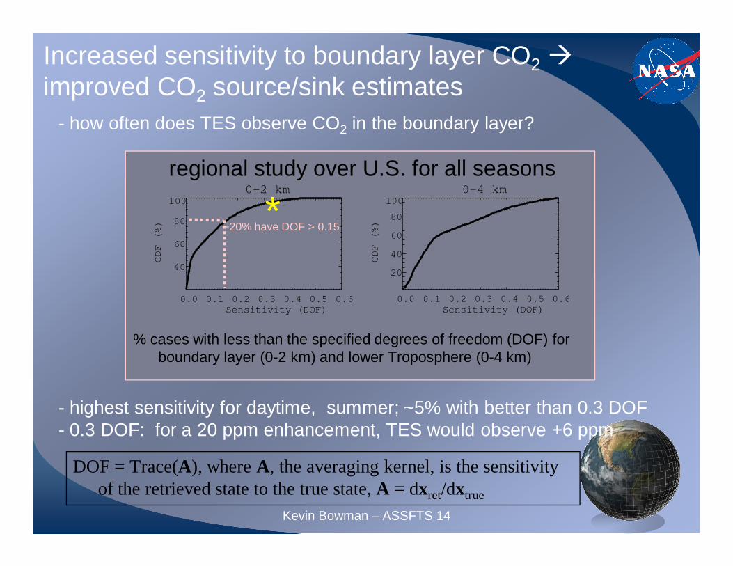
Increased sensitivity to boundary layer CO2�improved CO2 source/sink estimates

- how often does TES observe CO2 in the boundary layer?

0-2 km

0.0 0.1 0.2 0.3 0.4 0.5 0.6

Sensitivity (DOF)

40

60

80

100

CDF (%) ~20% have DOF > 0.15*

% cases with less than the specified degrees of freedom (DOF) for boundary layer (0-2 km) and lower Troposphere (0-4 km)

DOF = Trace(A), where A, the averaging kernel, is the sensitivity of the retrieved state to the true state, A = dxret/dxtrue

0-4 km

0.0 0.1 0.2 0.3 0.4 0.5 0.6

Sensitivity (DOF)

20

40

60

80

100

CDF (%)

- highest sensitivity for daytime, summer; ~5% with better than 0.3 DOF- 0.3 DOF: for a 20 ppm enhancement, TES would observe +6 ppm

regional study over U.S. for all seasons


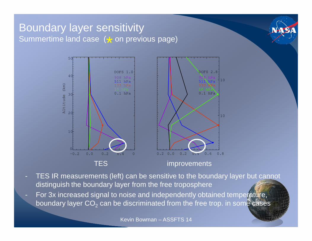
Boundary layer sensitivitySummertime land case ( on previous page)

TES improvements

- TES IR measurements (left) can be sensitive to the boundary layer but cannot distinguish the boundary layer from the free troposphere

- For 3x increased signal to noise and independently obtained temperature, boundary layer CO2 can be discriminated from the free trop. in some cases

3

-0.2 0.0 0.2 0.4 0.6

0

10

20

30

40

50

Altitude (km)

100

10

DOFS 1.0


3

-0.2 0.0 0.2 0.4 0.6 0.8

0

10

20

30

40

50

100

10

DOFS 2.8


*


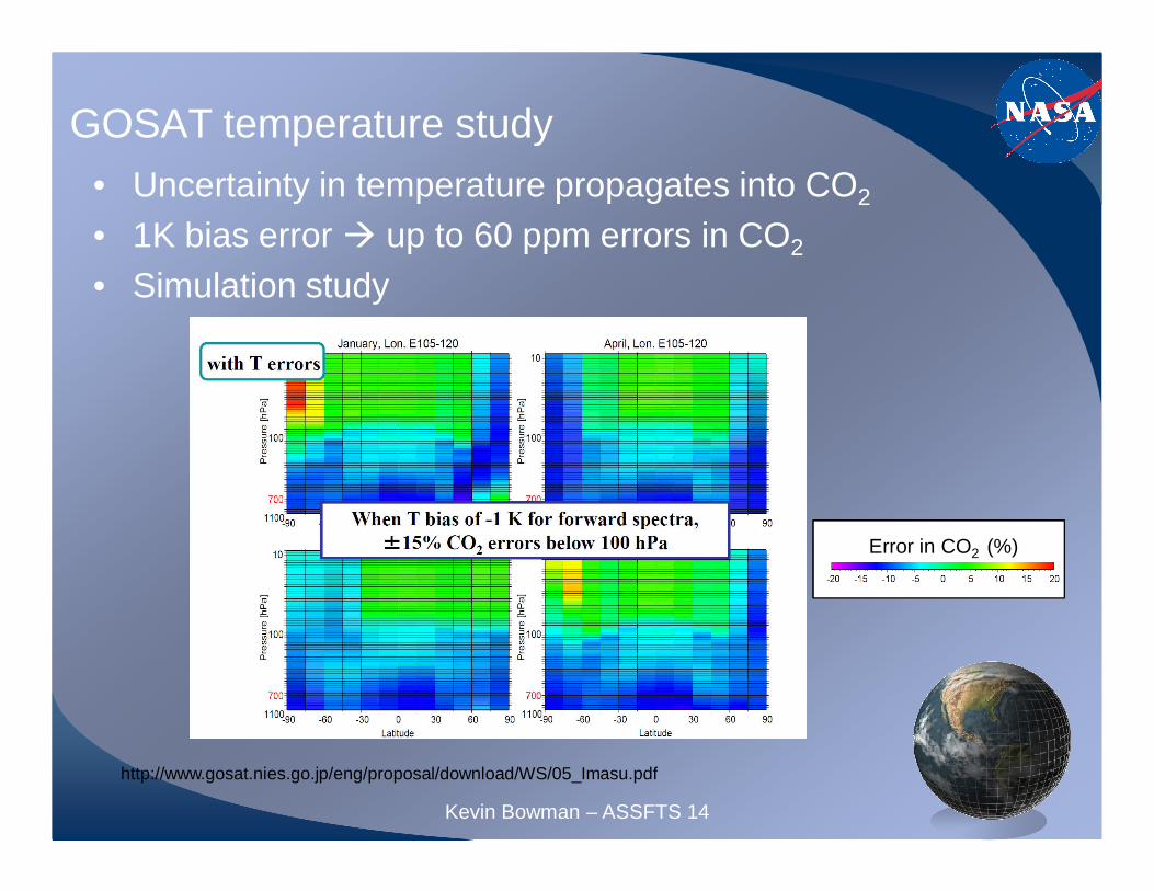
GOSAT temperature study• Uncertainty in temperature propagates into CO2

• 1K bias error � up to 60 ppm errors in CO2

• Simulation study

Error in CO2 (%)

http://www.gosat.nies.go.jp/eng/proposal/download/WS/05_Imasu.pdf


tes characterization for carbon cycle science ppt overview factors that affect co 2 source and sink...

Documents