terminal ballistics of composite panels and verification
TRANSCRIPT

Terminal Ballistics of Composite Panels
and Verification of Finite Element Analysis
by
Jonathan Scott Grupp
A thesis submitted to the Graduate Faculty of
Auburn University
in partial fulfillment of the
requirements for the Degree of
Master of Science
Auburn, Alabama
August 6, 2011
Keywords: ballistic impact, LS-DYNA, composites
Copyright 2011 by Jonathan Scott Grupp
Approved by
David Beale, Chair, Professor of Mechanical Engineering
Royall Broughton, Professor Emeritus of Polymer Fiber Engineering
Pradeep Lall, Thomas Walter Professor of Mechanical Engineering

ii
Abstract
Composite materials are becoming more prevalent in a wider range of applications due to the
inherent advantages afforded by their strength to weight ratio over more traditional engineering
materials such as metals. As such, composite materials are being exposed to a wider range of operating
environments. The aerospace sector has utilized composite materials for several decades to also benefit
from the weight savings such as increased fuel efficiency and vehicle range. These operating
environments for aerospace vehicles are hostile where fragments or projectiles can either penetrate or
perforate the composite material fuselage potentially damaging critical electronic and control
components and leading to catastrophic vehicle failure. Significant research efforts have been made
towards modeling the impact phenomena to develop the energy absorption capabilities of the
composite materials through the use of several different approaches including empirical correlation
through experimental testing, analytical methods, and numerical methods.
The research utilized both experimental and Finite Element methods to establish the energy
absorption capabilities of carbon fiber/epoxy laminate composite panels of different thicknesses to the
impact of a blunt-faced cylindrical 316 Stainless Steel projectile at different angles of obliquity. A total of
4 test matrices were performed which includes 0°, 30°, and 45° obliquity at 0.08” panel thickness, and 0°
obliquity at 0.18” panel thickness. An experimental accelerator was developed to accelerate the
projectile to prescribed velocities or energy levels. The impacting and residual velocities were measured
using a high speed video camera. The experimental data was used to create a correlation between
impacting and residual velocity for each of the test matrices.

iii
At high strain rates and upon the initiation of damage, composite materials exhibit a softening
behavior where the stiffness and rigidity of the composite are reduced successively as damage
propagates. The material model utilized in the Finite Element model is an orthotropic model with
progressive damage using a variation of Hashin’s failure criteria. The damage model is based on the
Matzenmiller (MLT) damage approach and uses damage softening parameters. Since current
experimental methods can yield a wide range of values for the damage softening parameters, a
parametric study was performed to calibrate the parameters using the experimental velocity correlation
of the 0° obliquity, 0.08” panel thickness test matrix. The calibrated material model was then used to
model the other three test matrices. The Finite Element model robustness was validated for the
extrapolated cases and was in good agreement with the experimental data.

iv
Acknowledgements
Special thanks must be made to the following individuals: Our research sponsors Matt Triplett,
Brent Deerman, Devin Chamness, and Dustin Clark. Without their support and advice, this research
would not be possible. Devlin Hayduke and Rich Foedinger at Material Sciences Corporation (MSC) for
providing a license to use the LS-DYNA MAT_COMPOSITE_DMG_MSC material model (MAT_162) and
the associated educational literature and presentation regarding the material model theory and
application. Dr. David Beale and Dr. Royall Broughton for providing the guidance and resources needed
to complete the research. Last but not least my family and friends for their continued support during my
educational pursuit.

v
Disclaimer Statement
This information product has been reviewed and approved for public release. The views
expressed herein are those of the author and do not reflect the official policy or position of the
Department of the Army, Department of Defense, or the U.S. Government.

vi
Table of Contents
Abstract ......................................................................................................................................................... ii
Acknowledgements ..................................................................................................................................... iv
Disclaimer Statement .................................................................................................................................... v
Table of Contents ......................................................................................................................................... vi
List of Figures ............................................................................................................................................... ix
Chapter 1: Introduction ................................................................................................................................ 1
Research Scope ......................................................................................................................................... 1
Impact Dynamics ....................................................................................................................................... 1
Finite Element Method and LS-DYNA ....................................................................................................... 6
Composite Materials Background ........................................................................................................... 10
Chapter 2: Experimental Setup ................................................................................................................... 13
Gas Gun Design ....................................................................................................................................... 13
Sabot Design ........................................................................................................................................... 15
Barrel Design ........................................................................................................................................... 16
Velocity Measurement Systems ............................................................................................................. 16
Gun Design Implementation ................................................................................................................... 17
Gun Design Overview .......................................................................................................................... 17
Performance Characteristics ............................................................................................................... 18
Velocity Measurement System Implementation .................................................................................... 20
High Speed Video Camera System ...................................................................................................... 20
vii
Velocity Measurements ...................................................................................................................... 22
Sabot Design Implementation ................................................................................................................ 24
Design Overview ................................................................................................................................. 24
Sabot Design Validation ...................................................................................................................... 28
Chapter 3: Impact Testing, Material Characterization, and Finite Element Analysis ................................. 31
Impact Testing ......................................................................................................................................... 35
Testing Results ........................................................................................................................................ 36
Experimental Characterization of Composite Panels ............................................................................. 36
Tensile Testing .................................................................................................................................... 37
Tensile Testing: Off-Axis Shear ............................................................................................................ 38
Compressive Testing ........................................................................................................................... 40
Finite Element Model Overview ............................................................................................................. 42
Model Geometry and Mesh Generation ............................................................................................. 42
Contact Elements ................................................................................................................................ 45
Projectile Material Model ................................................................................................................... 47
Composite Material Model ................................................................................................................. 48
Finite Element Simulations ..................................................................................................................... 56
Parametric Study: 5 Layer Panel, 0° Obliquity .................................................................................... 57
5 Layer Composite Panel, 30° Obliquity .............................................................................................. 64
10 Layer Composite Panel, 0° Obliquity .............................................................................................. 64
Qualitative Model Response ................................................................................................................... 65
5 Layer 0° Obliquity, No Perforation – Test Case 5 ............................................................................. 65
5 Layer 0° Obliquity, 20% Velocity Reduction – Test Case 6 ............................................................... 70
Conclusion ............................................................................................................................................... 74

viii
References .............................................................................................................................................. 76
Appendix A: Composite Laminate Orientation Code .................................................................................. 79
Appendix B: Experimental Characterization Data ...................................................................................... 80
Appendix C: S-2 Glass Material Model ........................................................................................................ 82
Appendix D: LS-Dyna Input File ................................................................................................................... 83

ix
List of Figures
Figure 1: Stress-Strain Curve at High Pressures (Nicholas et al, 1990) ......................................................... 2
Figure 2: Wave Effects in Long-Rod Penetration (Wright, 1983) .................................................................. 3
Figure 3: Eight Node Hexahedral Element (LSTC, 2006) ............................................................................... 7
Figure 4: Push vs. Pull Sabot (Stilp, 1990) ................................................................................................... 15
Figure 5: Experimental Gun ........................................................................................................................ 18
Figure 6: Experimental Pressure vs. Velocity Correlation ........................................................................... 19
Figure 7: Projectile Impact Location ........................................................................................................... 20
Figure 8: High Speed Video Camera Used for Velocity Measurements ...................................................... 21
Figure 9: Composite Panel Impact with Spherical Projectile ...................................................................... 22
Figure 10: Metric Board Used for High Speed Video Camera Calibration .................................................. 23
Figure 11: Capturing Pixel Coordinates For Velocity Measurements ......................................................... 24
Figure 12: CAD Representation of Sabot .................................................................................................... 25
Figure 13: Actual Sabot with Spherical Projectile ....................................................................................... 26
Figure 14: Assembled Sabot ........................................................................................................................ 26
Figure 15: Prototype Shear Jig Developed By Author ................................................................................. 27
Figure 16: Prototype Shear Mounted in Drill Press .................................................................................... 27
Figure 17: Projectile Trajectory Deviations (Zukas,1990) ........................................................................... 28
Figure 18: Sabot Validation using Blunt Cylinders ...................................................................................... 29
Figure 19: Sabot Stripper Plates .................................................................................................................. 30
Figure 20: V50 and the Zone of Mixed Results (Silsby, 1987) ..................................................................... 32

x
Figure 21: Non-Perforating Pyramidal Protrusion, Back of Composite Panel ............................................ 33
Figure 22: Close-up of Non-Penetrating Pyramidal Protrusion .................................................................. 34
Figure 23: Non-Penetrating Pyramidal Protrusion, Side View .................................................................... 34
Figure 24: 77.2% Velocity Reduction Pyramidal Protrusion, Back of Composite Panel ............................. 34
Figure 25: Close-up of 77.2% Velocity Reduction Pyramidal Protrusion .................................................... 35
Figure 26: 77.2% Velocity Reduction Pyramidal Protrusion, Side View ...................................................... 35
Figure 27: Impact Test Data Summarization Matrix ................................................................................... 36
Figure 28: Composite Material Directions in the Global Coordinate System (Adams et. al, 2003) ............ 37
Figure 29: Representation of Tabbed Sample (Adams et. al, 2003) ........................................................... 38
Figure 30: D3039 Tensile Test Results Summary (MSC) ............................................................................. 38
Figure 31: {0/90}s D3518 Test, Approximation for Shear Modulus ............................................................ 40
Figure 32: Sketch of CLC test fixture (Adams et al 2003) ............................................................................ 41
Figure 33: CLC test fixture (Adams et al 2003) ............................................................................................ 42
Figure 34: D6641 Compressive Test Results Summary (MSC) .................................................................... 42
Figure 35: Q4 Shell Element Plane Used to Generate Solid Elements ........................................................ 43
Figure 36: Representation of Test Sample Holder with Composite Panel (AMRDEC, 2010) ...................... 44
Figure 37: Boundary Conditions of Composite Panel ................................................................................. 45
Figure 38: Cylindrical Projectile Geometry and Mesh ................................................................................ 45
Figure 39: Projectile/Composite Panel Contact Element ........................................................................... 46
Figure 40: Composite Panel Interface Contact Element ............................................................................. 47
Figure 41: MAT_PLASTIC_KINEMATIC Projectile Material Model .............................................................. 47
Figure 42: MAT_PLASTIC_KINEMATIC Hardening Theory........................................................................... 48
Figure 43: MAT_COMPOSITE_DMG_MSC Composite Panel Material Parameters .................................... 49
Figure 44: Definition of AOPT=2 Material Coordinates (Hayduke, 2010) ................................................... 50
xi
Figure 45: Damage Parameters Baseline Comparison ................................................................................ 58
Figure 46: Baseline Variable Matrix ............................................................................................................ 58
Figure 47: AM1, AM2 Fiber Softening Effects Comparison ........................................................................ 59
Figure 48: Fiber Softening Variable Matrix ................................................................................................. 59
Figure 49: AM3 Fiber Crush, Punch Shear Comparison .............................................................................. 60
Figure 50: Fiber Crush, Punch Shear Variable Matrix ................................................................................. 60
Figure 51: AM4 Matrix, Delamination Comparison .................................................................................... 61
Figure 52: Matrix, Delamination Variable Matrix ....................................................................................... 61
Figure 53: Mesh Comparison ...................................................................................................................... 62
Figure 54: Mesh Comparison Variable Matrix ............................................................................................ 63
Figure 55: 5 Layer Composite 0° Obliquity Model Results .......................................................................... 63
Figure 56: 5 Layer Composite 30° Obliquity Model Results........................................................................ 64
Figure 57: 10 Layer Composite 0° Obliquity Model Results........................................................................ 65
Figure 58: Test Case 5 Damage, Front View ............................................................................................... 66
Figure 59: Test Case 5 Damage Close Up .................................................................................................... 66
Figure 60: Test Case 5 Side View ................................................................................................................. 67
Figure 61: Test Case 5 Video Stills, No Perforation, Projectile Ricochets ................................................... 68
Figure 62: LS-DYNA Video Stills, Side View - Test Case 5 ............................................................................ 69
Figure 63: LS-DYNA Projectile Velocity Plot – Test Case 5 .......................................................................... 69
Figure 64: Measurement Nodes for Deflection, Test Case 5 ...................................................................... 70
Figure 65: Test Case 5 Deflection ................................................................................................................ 70
Figure 66: Test Case 6 Damage ................................................................................................................... 71
Figure 67: Test Case 6 Damage Close Up .................................................................................................... 71
Figure 68: Test Case 6 Video Stills, 20.15% Velocity Reduction ................................................................. 72

xii
Figure 69: LS-DYNA Video Stills, Side and Back Views - Test Case 6 ........................................................... 73
Figure 70: D3039 Tensile Test Data, {0/90}s ............................................................................................... 80
Figure 71: D3039 Tensile Test Data, {0/90/45/-45}s, Quasi-Isotropic ........................................................ 80
Figure 72: D6641 Compressive Test Data, {0/90}s...................................................................................... 81
Figure 73: D6641 Compressive Test Data, {0/90/45/-45}s, Quasi-Isotropic ............................................... 81
Figure 74: S-2 Glass Composite Material Model (Xiao et al, 2005) ............................................................ 82

1
Chapter 1: Introduction
Research Scope The research focus is to establish the energy absorption capabilities of carbon fiber/epoxy
laminate composite materials through the use of both experimental and numerical methods. A single
stage gas gun accelerator was developed to propel the projectile. LS-DYNA Finite Element solver was
used throughout the research for numerical solutions. Chapter 1 establishes the fundamentals of impact
dynamics, Finite Element Methods, and composite material behavior. Chapter 2 establishes
experimental methods used in impact analysis. Chapter 3 presents the experimental test results, the
development of the Finite Element model, and the model agreement to experimental results.
Impact Dynamics Impact dynamics is the study of the phenomena surrounding the collision of two or more bodies
whose deformation is considerable and thus the bodies cannot be considered perfectly rigid. Two
primary features that separate impact events from those of quasi-static mechanics are the inertial
effects and the stress wave propagation in the colliding bodies (1). Typically the experimental means to
study an impact event is through the acceleration of one body, a projectile, at a given body, a target,
that is constrained to be fixed in space. Also important to the accurate modeling of impact dynamics of
deformable bodies is the characterization of the material behavior in both the quasi-static and high
strain regimes, failure criteria at high strain rate, and penetration mechanics.
Penetration mechanics is the study regarding the penetration and perforation of the target, and
the underlying phenomena related to the observed behavior. Penetration is defined as when the
projectile breaks the interface at the contact area on the target and enters without fully punching
through the target (2). Perforation occurs when the projectile completely punches through the target,
exiting the other side (2). Penetration mechanics takes into account the stress wave propagation in both

2
the projectile and the target and the resulting deformations and failure due to the elastic, plastic, and
possible shock waves (1) (2). For low velocities, the pressure exerted on the target may be low enough
to not exceed the yield strength such that only elastic waves are generated moving at the speed of
sound of the material. At higher velocities, sufficient pressure could exceed the yield strength to also
generate plastic waves moving at the speed of sound in the material. Based on the rate-independent
theory of plastic wave propagation, at even higher pressures the stress-strain curve goes from linear to
concave-up as shown in Figure 1 where is the maximum propagating stress (1). As a result higher
stress waves travel faster than lower amplitude waves and a single wave front forms to create a shock
wave (1). An example of the effect that the wave propagation has in both the target and projectile for
metallic material compositions is illustrated in Figure 2 (3).
Figure 1: Stress-Strain Curve at High Pressures (Nicholas et al, 1990)

3
Figure 2: Wave Effects in Long-Rod Penetration (Wright, 1983)
In order to understand and quantify the penetration phenomena, there are three main
approaches to analyzing impact events (2). These approaches include empirical methods through
experimental data, analytical methods involving the fundamental conservation laws with closed form
solutions derived from simplifying assumptions, and numerical methods often employing finite element
and finite difference methods (1). Each method will be explored in further detail in the ongoing
development.
Empirical methods seek to correlate several key factors to the experimental data and thus are
often intensive in the amount of testing required to obtain a good fit to the data (1). In addition the
empirical relationships cannot confidently be extrapolated beyond the bounds which they were formed.
This includes, but is not limited to, the material properties of the bodies, geometry of the overall body
and impact interface, and the relative trajectory and velocity for the collision. A well-known example of
the empirical approach is the THOR equations developed from experiments of various projectile
geometries and various material compositions (2). The THOR equations can be represented as in Eqn 1
and Eqn 2 where and are the residual and striking velocities in feet per second, h is the target
material thickness in inches, A is the impact area in square inches, and are the residual and initial

4
mass of the projectile in grains, and ci and di, i=1 to 5, are correlation coefficients for the variety of test
parameters (2) (4) (5). The coefficients are calculated for specific cases and are tabulated. Due to the
nature of the development of the empirical relationships only very specific combinations of factors are
available with no practical or accurate method to extrapolate beyond the bounds of the coefficients.
Also since only very specific portions of the response are considered in the empirical relations, not much
fundamental understanding can be gained about other contributing factors in the impact event (1).
Eqn 1
Eqn 2
Analytical approaches typically use a combination of the three conservation laws in order to
develop a relation for a particular aspect. Often a single parameter is developed at a time as multiple
parameters in analytical approaches can become difficult to solve (2). The most often referenced is the
Recht-Ipson formula which solves for the residual velocity and is based on Impulse-Momentum and
Work-Energy balances. The development by Recht is included in the aforementioned order in Eqn 3 and
Eqn 4 where the variables are defined in Eqn 7 (6). Eqn 4 can be further simplified by substituting the
relations developed by Recht for and , defined in Eqn 7 (6). The characteristic velocity is often
determined through experimental tests by using the , ballistic limit velocity. is defined as the
velocity at which there is a 50% likelihood that perforation will occur (2). A good agreement can be
obtained to experimental data but a characteristic velocity must be determined (7). Although a good
agreement can be attained using analytical approaches, an incomplete picture of the impact event
results.
Eqn 3

5
Eqn 4
[ ⁄ ]
Eqn 5
[ ⁄ ]
Eqn 6
Where:
– initial projectile mass
– residual projectile mass
m – mass driven from target
– residual velocity of projectile and mass, m Eqn 7
I – impulse transmitted to target
– elastic/plastic deformation energy due to the impact of and m
– elastic/plastic deformation energy due to constraint of mass, m, to the target
– characteristic velocity
Β – change in trajectory angle between pre- and post-impact
Numerical approaches can overcome some of the limitations related to the level of
understanding of the underlying penetration mechanics. Instead of solving for the actual impact event, a
discretized solution is solved which can yield a high level of agreement to experimental data provided
that the model is representative of reality. Finite Element methods are currently the most common
numerical solution in use for penetration modeling. Within the past decade, the advent of increased
computing power alongside the further refinement of the commercial Finite Elements codes has allowed
increasingly complex simulations that are more representative of reality. Finite Element simulations can

6
allow a better level of understanding regarding the penetration mechanics and also some predictive
capabilities. As such, the Finite element approach will be utilized for this research and the
aforementioned assertions will be examined.
Finite Element Method and LS-DYNA The Finite Element Method is a methodology to numerically solve a field problem where a
distribution of dependent variables is mapped in space (8). It is formed on the basis of continuum
mechanics where a body is assumed to be continuous and homogenous and therefore uniform in
material behavior. In the Finite Element method a continuous body is discretized into a finite number of
elements and degrees of freedom where the field quantity is calculated at the nodes. Each of the
elements contains a prescribed number of nodes as demonstrated in the hexahedral element of Figure
3. The array of elements in the continuous body or structure is referred to as the model mesh (8). For
structural problems the displacements of the nodes are used to calculate the strains and stresses at
each of the nodes and elements. The continuity between the elements is provided by approximation or
shape functions (9). There are several available commercial Finite Elements codes available to apply to
an array of problem types that include heat transfer, structural dynamics, wave propagation, and fluid
dynamics. Some of the popular Finite Element solvers include ABAQUS, ANSYS, MSC DYTRAN, MSC
NASTRAN, and LS-DYNA. LS-DYNA will be used in this research due to its’ suitability to solve for highly
dynamic events such as ballistic impact which will be established in the ongoing section.

7
Figure 3: Eight Node Hexahedral Element (LSTC, 2006)
Based on Newton’s 2nd Law, , the Finite Element structure can be represented as that in
Eqn 8 where { } is the nodal degree of freedom matrix, [ ] is the consistent mass matrix, [ ] is the
consistent damping matrix, and { } and { } are external and internal force matrices (8). If linear
stiffnesses occur for the given material of the structure then Eqn 8 can be represented as Eqn 9 where
[ ] is the stiffness matrix (8).
[ ]{ } [ ]{ } { } { } Eqn 8
[ ]{ } [ ]{ } [ ]{ } { } Eqn 9
In order to solve the 2nd order differential equations represented by Eqn 8, several different
integration techniques are commonly used and can be classified as either explicit or implicit (8). The two
main methods are the Newmark method, an implicit method, and the central difference method, an
explicit method (8). As will be outlined, the appropriate integration method selected will depend on the
problem type.
The Newmark method is as follows in Eqn 10 and Eqn 11 where λ and β are factors that control
accuracy, numerical stability, and dampening, and n and n+1 are the current and next time steps (8).

8
{ }
{ } ( { }
{ }
)
Eqn 10
{ } { } { }
( { }
{ }
)
Eqn 11
Typically commercial software codes use implicit methods that are unconditionally stable where Δt can
be as large as desired but at the cost of accuracy (8). LS-DYNA by default uses an explicit integration
method (10). LS-DYNA has evolved over the years and has included the functionality of its’ predecessors
DYNA2D and DYNA3D but has also recently included the implicit integration capabilities of NIKE3D (10)
(11). The general principle of the implicit integration used in LS-DYNA is represented in Eqn 12 (11). Eqn
12 implies that the global stiffness matrix is calculated and inverted to be applied to the nodal force
balance to calculate the displacement at the next time step (12).
[ ]{ }
[ ]{ } { } { } [ ]{ }
Eqn 12
Two problems result from Eqn 12, a non-linear and linear problem (11). The nonlinear problem involves
determining the displacement in which { } { } by utilizing iterative Newton-Raphson methods
(12). The linear problem involves solving the linear system of equations [ ]{ } { } for each
iteration of the nonlinear problem (12). Due to the inversion of the stiffness matrix and solving of the
nonlinear and linear problems for each iteration of the Newton-Raphson method, considerable
computational resources are required for the implicit integration method. As such implicit integration is
better suited to structural dynamics problems which can be classified as either static or quasi-static (8).
The central difference method can be represented as Eqn 13 and Eqn 14 (8).
{ }
{ } { }
Eqn 13

9
{ }
{ } { } { }
Eqn 14
Explicit methods are conditionally stable depending on the size of the time step, Δt. The calculation will
remain numerically stable as long as the time step does not exceed the critical time step, , defined
as the Courant condition (8). The time step should not exceed the amount of time required for a stress
wave to travel through the smallest element in the mesh (13). The critical time step relationship is
shown in Eqn 15 where is the characteristic length or the distance across the smallest element and c
is the speed of sound through the material or the speed of the tensile stress wave (8) (13).
√ ⁄
Eqn 15
LS-DYNA automatically calculates the time step for simulations using the explicit integration algorithm
but also does allow the user some control over the time step (10). The user can either explicitly define
the time step or can utilize the LS-DYNA calculation along with a factor to scale the time step down (10).
As shown in Eqn 16 where TSSF is the time step scale factor (13) (14). The default value for TSSF is 0.9
and the user can further adjust the factor lower to better ensure numerical stability but at a
computational expense for the increased number of computing cycles (13) (14).
Eqn 16
Each time step does not require considerable computational resources but since each time step is small,
many time steps are required to complete the simulation (8). Therefore explicit integration methods are
more suitable to wave propagation problems such as the present problem of ballistic impact. The
general scheme of the explicit integration algorithm used In LS-DYNA can be represented as in Eqn 17
(11) (12). Eqn 17 states that the internal and external forces are summed at each node and the nodal
acceleration is calculated by dividing the summation by the nodal mass (11) (12). The simulation is

10
advanced by integration of the acceleration with respect to time to solve for the nodal velocity and
displacements (12).
[ ]{ } { } { }
Eqn 17
Composite Materials Background Composite materials are defined as a material that incorporates two or more different base
materials to form a third material (15). The resulting material often exhibits different material behavior
from the base materials which is resultant of the formation and interaction of the base materials.
Composite materials cover a wide array of material types that can include fibrous composites,
particulate composites, laminated composites, and a combination thereof (15). Common to all of the
different permutations possible in composites is a binding material which is often referred to as the
matrix material (15). The matrix material serves to hold the fibers, particles, or fabric layers in a specific
orientation to provide the capability to support loads and transfer stress. Oftentimes the matrix serves
as a protection layer against abrasion or material degradation to environmental influences such as
chemical or UV radiation exposure. Common matrix materials include polymers, metals, ceramics, and
carbon (15). Polymers can be classified as a thermoplastic, rubber, or thermoset (15). The major
difference between the different classifications are the level of crosslinking of the molecules that form
the polymer and are listed in ascending order of degree of crosslinking with thermoplastics having the
least (15). As such thermoplastics can be reprocessed because not as many permanent bonds have been
formed while thermosets cannot be reconstituted (15).
Relevant to this research are laminated composites using a thermoset polymer matrix or epoxy.
Laminated composites can be assembled by means of several different methods. Some of these include
filament winding, tape laying, and fabric laying (15). Typically the filament, tape, or fabric is impregnated
with an epoxy that is allowed to enter a semi-cured state and is typically regarded as a prepreg. The use

11
of prepreg allows for easier assemblage of the composite during the winding or laying process and also a
consistent distribution of the epoxy. The winding or laying processes allow for control of the filament or
fiber orientation and is often termed the lay-up pattern (15). As such, the desired stiffness, rigidity, and
strengths can be obtained in the desired material directions as dictated by design criteria. In addition, in
the laying processes either unidirectional or weave fabrics can be used which offers further control over
the material behavior relative to the material directions. Following the assembly of the laminate the
epoxy crosslinking is obtained through a curing process where heat and pressure is applied to the
composite during a designated time period. The curing process also ensures the successful migration of
any trapped air pockets in the epoxy to minimize the possibilities of voids which can cause weak points
or stress concentrations in the composite material.
As mentioned previously the orientation of the fabric or filament dictates the stiffness, strength,
and rigidity in the material coordinate system. Accordingly, laminated composite materials exhibit
anisotropic material behavior (15). For linear elastic composites, the compliance matrix, , from the
strain-stress relations in Eqn 18 consists of 36 terms of which 21 are independent as shown in Eqn 19
(15). Depending on the lay-up pattern, the compliance matrix can be further reduced depending on the
material symmetry which include monoclinic, orthotropic, transversely isotropic, or even isotropic.
Using standard laminate code, which is summarized in Appendix A: Composite Laminate Orientation
Code, a {0/90}s construction of plain weave carbon fiber fabric is used in the present research. The
{0/90}s can be assumed to exhibit orthotropic material behavior since the principal directions of the
lamina are aligned with the resulting principal directions of the composite laminate. By the assumption
of orthotropic material behavior, Eqn 19 reduces to Eqn 20 where 9 independent properties remain. In
later developments, Eqn 20 will be modified to include the softening behavior of composite materials
due to the high strain rates induced from ballistic impact.

12
{
31
23
12
33
22
11
}
[ ]
{
31
23
12
33
22
11
}
Eqn 18
[ ]
[
666564636261
565554535251
464544434241
363534333231
262524232221
161514131211
SSSSSS
SSSSSS
SSSSSS
SSSSSS
SSSSSS
SSSSSS
]
Eqn 19
[ ]
[
31
23
12
32
23
1
13
3
32
21
12
3
31
2
21
1
100000
01
0000
001
000
0001
0001
0001
G
G
G
EEE
EEE
EEE
]
Eqn 20

13
Chapter 2: Experimental Setup
Gas Gun Design There are several different types of projectile accelerators used in impact analysis studies such
as electrostatic and electromagnetic, explosive-based (shape charges), plasma, and gun accelerators
(16). However the most common accelerators are gas guns since the widest range of projectile
geometries, materials, and mass can be utilized. Gas guns operate on the principle that projectile
acceleration is provided from the rapid expansion of gas in a given volume. As the gas expands, a force is
exerted on the projectile which accelerates it to a desired impact velocity or energy level. There are
three primary energy delivery systems commonly used in gas gun design: single stage pressurized gas-
based and propellant-based, and two stage gas guns (16). The operating principle varies slightly for each
of the aforementioned energy delivery systems. Propellant-based systems utilize a given amount of
propellant, typically a powder, to accelerate the projectile. Generally a controlled ignition event starts a
chemical reaction in the propellant which rapidly generates gas. The rapid expansion of the driving gas
accelerates the projectile to a desired impact velocity or energy level. The control mechanisms for the
impact velocity are the amount of propellant used and the rate at which the propellant generates gas. In
practice, propellant-based systems are better suited towards higher velocity regimes. A two stage gas
gun utilizes a propellant-based system in the first stage. The propellant in this system drives a piston
which compresses and heats the driving gas. Once a specific pressure value is reached, a diaphragm
bursts and allows for the driving gas to accelerate the projectile down the barrel (16).
Due to the extra safety requirements surrounding the use of propellant, a single stage
pressurized gas system was utilized for this research. Pressurized gas-based systems rely on a gas at a
given pressure and high speed valve to regulate the pressurized gas. When the valve is opened the
pressurized gas expands to reach equilibrium pressure to the atmosphere and accelerate the projectile.
The effectiveness of the gun is related to the response time of the high speed valve. The impact velocity

14
can be controlled through various means: selection of gas, pressure of gas, temperature of gas, length of
the barrel, and cross-sectional areas of the pressure reservoir and barrel. The impact velocity range can
be controlled by the use of gases of different densities or molecular weight and correspondingly
different speeds of sound (17). The most common gases used are helium, nitrogen, and air (17). Firstly,
the speed at which a projectile can move in a given gas medium is related to its compressibility and
inertia, commonly represented as the Mach number:
Eqn 21
where V is the flow speed and c is the speed of sound (17) (18). The flow of the projectile is often
divided into several regimes based on Mach number (18). Secondly, the impact velocity can further be
controlled by the pressure and temperature at which the gas is released. The initial pressure dictates the
mechanisms that affect the projectile acceleration. Since the gas, pressure, and valve speed can be
controlled, pressurized gas guns offer good control to the end-user for the desired impact energy.
Based on Newton’s Law of Motion, Seigel developed a basic relationship to calculate a
theoretical maximum muzzle speed, , for a given gas gun:
√
Eqn 22
where is the base pressure, A is the cross-sectional area of the barrel, L is the length of the barrel, and
m is the mass of the projectile (17). This relationship is considered an approximation because it does not
include friction effects against the interior barrel wall or the compressibility effects of the gas in front of
the projectile and the base pressure is considered to remain constant during projectile acceleration. As a
guideline the muzzle velocity of an actual gun will not be more than half the theoretical prediction (17) .
15
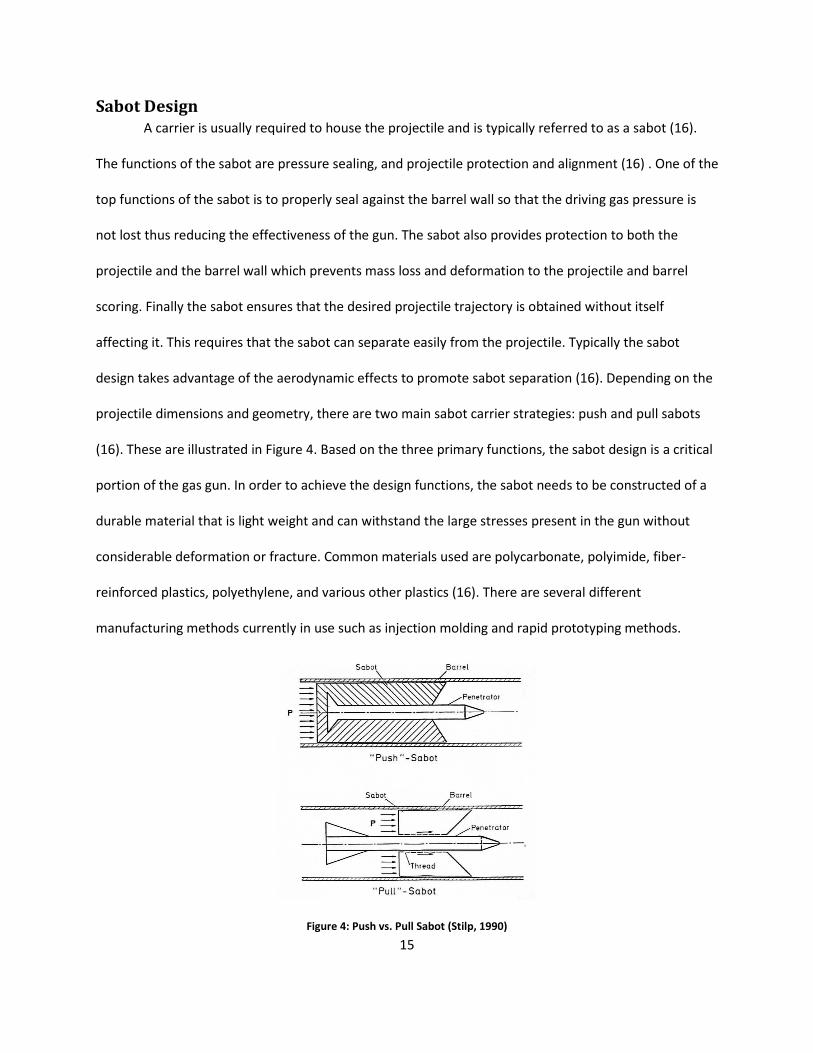
Sabot Design A carrier is usually required to house the projectile and is typically referred to as a sabot (16).
The functions of the sabot are pressure sealing, and projectile protection and alignment (16) . One of the
top functions of the sabot is to properly seal against the barrel wall so that the driving gas pressure is
not lost thus reducing the effectiveness of the gun. The sabot also provides protection to both the
projectile and the barrel wall which prevents mass loss and deformation to the projectile and barrel
scoring. Finally the sabot ensures that the desired projectile trajectory is obtained without itself
affecting it. This requires that the sabot can separate easily from the projectile. Typically the sabot
design takes advantage of the aerodynamic effects to promote sabot separation (16). Depending on the
projectile dimensions and geometry, there are two main sabot carrier strategies: push and pull sabots
(16). These are illustrated in Figure 4. Based on the three primary functions, the sabot design is a critical
portion of the gas gun. In order to achieve the design functions, the sabot needs to be constructed of a
durable material that is light weight and can withstand the large stresses present in the gun without
considerable deformation or fracture. Common materials used are polycarbonate, polyimide, fiber-
reinforced plastics, polyethylene, and various other plastics (16). There are several different
manufacturing methods currently in use such as injection molding and rapid prototyping methods.
Figure 4: Push vs. Pull Sabot (Stilp, 1990)

16
Barrel Design The barrel is another critical component to the gas gun. The barrel is typically constructed from
high strength steel with a sufficient wall thickness to handle the operating pressures. As is demonstrated
from the equation developed by Seigel shown earlier, the cross-sectional area and length of the barrel
play a large role in the maximum muzzle velocity obtained and thus are dependent on the specific
experiment design parameters. Generally a longer barrel is used for higher muzzle velocities. Depending
on the type of projectile, the barrel can utilize either a rifled or smooth bore (16). Rifling is a common
machining technique that adds helical grooves to the bore wall. As the projectile moves through the
barrel, the rifling induces spin onto the projectile which provides for a much straighter trajectory.
However, depending on the projectile, induced spin may not be desirable for the impact event since
orientation to the impact surface may need to be controlled in the experiment. There are several
machining or manufacturing processes used to create a high precision barrel. Generally a barrel is
machined by honing the interior surface to the desired diameter (16). For extremely long barrels, several
tube sections have to be attached due to the limitation of the depth the honing process can occur on a
given section (16).
Velocity Measurement Systems Common empirical analysis techniques utilize impulse-momentum and work-energy balances (6)
(1). As such, velocity is one of the primary outputs for characterizing the energy absorption capabilities
of a given sample. Projectile velocity is measured both pre- and post-impact and typically termed impact
and residual velocity to complete the momentum and energy balances. There are several different
methodologies used to measure velocity which include chronographs, laser interferometry, high speed
photography, and high speed cinematography (16) (19). Common to all techniques is that the velocity is
calculated by using a known distance between points and a known time interval. In terms of cost,
chronographs are the cheapest to implement into an experimental set-up while the other techniques

17
require much more expensive equipment. High speed photography and cinematography give the added
benefit of additional information regarding the impact event such as projectile orientation to the target,
the particle distribution resulting from the impact, and the trajectory of the projectile post-impact. In
addition high speed photography and cinematography can allow for better measurement of the
projectiles residual velocity since the projectile trajectory may change post-impact. However special
consideration must be made regarding the lighting available to obtain proper exposure during the
impact event. For very high velocity impact events, a special trigger system is used to operate a flash
system to provide a very intense light to illuminate the event (16). In the case of high speed video
cameras, a very high velocity requires very fast shutter speeds and frame rates to provide a clear
picture.
Gun Design Implementation
Gun Design Overview
During the course of the research, an experimental accelerator for projectile impact was co-
developed with several Mechanical Engineering undergraduate design project groups. The primary
design directives were true trajectory, high accuracy and precision for impact location, and controllable
projectile speed up to 500 meters per second for a 0.5” diameter steel sphere. Based on current design
practices and the aforementioned design and safety requirements, a single stage pressurized-gas gun
design was selected. Since the composite panels were not expected to require energy levels beyond the
aforementioned design requirements, air pressurized by a compressor is used as the driving gas. The
system consists of a high pressure compressor, high pressure scuba tank, piping manifold, high speed
valve, and a smooth bore barrel as shown in Figure 5. The system is designed around a minimum safety
factor of 2 by using a maximum operating pressure of 1500 psi.

18
Figure 5: Experimental Gun
Performance Characteristics
Currently the usable velocity range is between 100 and 375 meters per second. A relationship
between the tank pressure and the impact velocity was developed experimentally. The velocities were
measured and calculated as documented in the Velocity Measurement System Implementation section.
As is shown in Figure 6, a logarithmic regression was used to best fit the velocity data. Beyond
approximately 600 psi the impact velocity does not increase and plateaus. Although frictional forces and
compressibility effects of the air in front of the projectile play a large role, it is suspected by the author
that the response time of the high speed valve is not fast enough to allow for a shock wave to aid in the
acceleration of the projectile. The current undergraduate design group is implementing a new valve
design that should reduce the current valve’s response time of 100 milliseconds.

19
Figure 6: Experimental Pressure vs. Velocity Correlation
As was mentioned in the Gun Design Overview section, impact location accuracy and precision
are part of the design parameters for the gun and also are highly important in ballistic experiments. By
striking in the center of the target for each of the test shots, the experimentalist can ensure that the
effect that the boundary conditions are comparable between each test and minimizes the chance the
boundary conditions affect the resulting data. In Figure 7, a location plot of the impact is provided for a
test consisting of 13 samples at various velocities in order to simulate an actual test matrix. From visual
inspection, both the precision and accuracy of the gun is high. The standard deviation for the impact
locations in both the x and y coordinates are 0.027” and 0.145” respectively. Reviewing the standard
deviations the y coordinate location is less precise but is expected as the amount the projectile drops is
related to the velocity at which it is traveling. The impact locations are no greater than a 0.14” radius
from center for a maximum striking zone area of . Based on this analysis, the interaction

20
effects between the impact location and the boundary conditions can be considered constant in
experimental testing.
Figure 7: Projectile Impact Location
Velocity Measurement System Implementation
High Speed Video Camera System
A high speed camera was made available for this research by the Polymer and Fiber Engineering
department. As highlighted in the Gas Gun Design section, high speed cinematography or video offers
multiple benefits other than output of velocity data such as particle fields created post impact. However
special considerations must be made regarding lighting for proper illumination of the impact event. For
this study, with the velocity ranges mentioned in the Performance Characteristics subsection, an array of
halogen lights were sufficient to provide the lighting necessary to record the impact event. In addition to

21
the lighting, a white opaque film was applied to the safety enclosure interior walls to increase the
reflectivity and improve the light distribution inside the enclosure.
Figure 8: High Speed Video Camera Used for Velocity Measurements
The camera used throughout the research is a NAC HotShot 512sc. It is capable of resolutions up
to 512 x 512 pixels and frame rates up to 200,000 frames per second (20). The camera is capable of full
resolution frames up to 5,000 frames per second and beyond that frame rate, the vertical resolution is
reduced (20). For the velocities being measured in the study, a frame rate of 10,000 frames per second
and shutter speed of 1/100,000 was found to be suitable settings for the camera. In Figure 9, video stills
from testing composite panels are shown. From the videos, the projectile can be clearly seen as well as
the trajectory pre- and post-impact. In the second still the particle distribution is clearly seen which can
be useful in the evaluation of the impact resistance of a given composite panel construction.

22
Figure 9: Composite Panel Impact with Spherical Projectile
Velocity Measurements
Using a high speed camera is relatively straight forward but additional steps must be taken to
ensure that the velocity measurements are accurate. The first consideration is the camera must be
properly aligned to the impact event which includes positioning the camera perpendicular to the
projectile trajectory, aligning to the impact location, and leveling the camera for no tilt relative to the
impact location. Lastly the camera must be calibrated to obtain the conversion factor for pixels to
distance. A common technique used is the implementation of a metric board as shown in the video still
in Figure 10. The metric board used in this research was a translucent plastic board with gridlines
measuring 2” x 1”, vertically and horizontally. The metric board is placed in the trajectory path and is

23
illuminated from backlighting with a halogen lamp. The camera software allows the user to select the
gridline points on the metric board to calibrate the camera for the position relative to the measurement
plane.
Figure 10: Metric Board Used for High Speed Video Camera Calibration
Once the camera is calibrated, videos can be recorded to collect velocity data. In order to
calculate the impact and residual velocities, data points consisting of pixel x and y coordinates and time
were collected from individual frames in the video and used to calculate the average velocity between
different spans. The pixel coordinates are selected at the leading edge of the projectile as shown in
Figure 11. In order to reduce induced error from the pixel selection process, at least 3 overlapping spans
were used to create an overall average value for each of the velocities.

24
Figure 11: Capturing Pixel Coordinates For Velocity Measurements
Sabot Design Implementation
Design Overview
The sabot developed is a three piece push design consisting of three main parts: the two sabot
halves and the interlocking rod. The design can readily handle solids of revolution such as spheres or
cylinders having various impact geometries such as blunt, conical, parabolic, and hemispherical. An
acetal plastic, trade name Delrin, was selected as the sabot material based on its strength
characteristics, low friction, and machinability. As can be seen in Figure 12 and Figure 13, an angled
ramp is added to promote sabot separation through aerodynamic forces. The interlocking rod maintains
the positioning of the two halves by preventing relative translation and also provides a pivot point for
sabot separation.

25
Figure 12: CAD Representation of Sabot
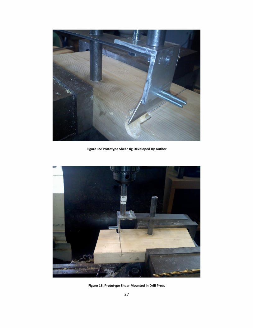
A low cost method, developed by the author, utilizes common machine shop equipment to
create the sabots’ design features. The manufacturing method consists of seven main operations listed
by equipment used and operation description:
1) Lathe - turn down a cylindrical rod of Delrin stock to the appropriate outer diameter
2) Lathe - drill to create the channel to house the projectile
3) Lathe - countersink aerodynamic ramp feature to aid in sabot separation
4) Drill press - drill channel for interlocking rod
5) Miter Saw - precut the sabot to allow for better sabot separation
6) Custom Shear Press - initiate a crack and create two sabot halves
7) Assemble three sabot pieces
The sawing and shear operations are highlighted in Figure 14. The author created a custom shear that
utilizes the mechanical advantage of a drill press to initiate a crack in the Delrin sabot as shown in Figure
15 and Figure 16. By using a shearing process, no material is lost and the sabot retains its cylindrical
cross section which ensures that proper sealing can be achieved against the barrel bore.

26
Figure 13: Actual Sabot with Spherical Projectile
Figure 14: Assembled Sabot
Shear Operation
Miter Saw Operation
27
Figure 15: Prototype Shear Jig Developed By Author
Figure 16: Prototype Shear Mounted in Drill Press

28
Sabot Design Validation
The high speed video camera was utilized to validate the performance of the sabot. For this
research project, blunt faced cylinders are the projectile geometry and validation was performed using
cylinders. Since we were limited to viewing in one plane, we will not consider that the roll and yaw of
the projectile but only the pitch as illustrated in Figure 17. As can be seen in the video stills of Figure 18,
the sabot starts to separate from the projectile at 4 feet from the muzzle and is fully separated from the
projectile. From several rounds of experimentation, the sabot design demonstrated consistent
separation from the projectile without affecting the trajectory or inducing pitch.
Figure 17: Projectile Trajectory Deviations (Zukas,1990)

29
Figure 18: Sabot Validation using Blunt Cylinders
Also evident from the video stills is that although the sabot separates from the projectile, the sabot
maintains the same general trajectory as the projectile and thus additional protection is needed to
protect the test sample. As seen in Figure 19, two sabot stripper plates were placed in front of the
impact location to ‘strip’ the sabot from the projectile. The first stripper plate is constructed of 12 gauge
sheet steel and the second plate is a 0.5” thick Lexan sheet. Lexan was selected for the second stripper
plate to allow for light to illuminate the impact location. Each stripper plate has a hole cut to allow only

30
the projectile to pass through the plate. The first stripper plate blocks most of the sabot but causes a
particle field due to the fracture of the Delrin upon impact. The second stripper plate blocks the sabot
particle field from impacting the test sample.
Figure 19: Sabot Stripper Plates
Steel Stripper Plate
Lexan Stripper Plate

31
Chapter 3: Impact Testing, Material Characterization, and Finite Element
Analysis Carbon fiber composites are currently being adopted into applications where a combination of
light weight and strength are needed. In many applications such as those in the aerospace sector, the
response to errant fragments and the resulting particle debris field is pertinent to evaluate a potentially
critical failure mode. The kinetic energy of resulting debris field can also cause further damage to
internal components such as structural elements and control systems. However experimental testing is
an expensive process to incur on several possible designs. In order to reduce the amount of
experimental testing needed, considerable effort is going towards a better understanding of the
underlying mechanics involved in terminal ballistics and accurately modeling the response using
numerical methods such as Finite Element methods (1).
In order to properly apply a numerical approach to model the impact event, experimental
testing is needed for model evaluation and validation. One of the common performance characteristics
in impact dynamics is the (6) (2) (21) (22). is defined as the velocity at which perforation of the
target occurs 50% of the time and as such is considered to be the threshold for the energy absorption
capabilities. There are several different methodologies to develop experimentally. The most
referenced are the Jonas-Lambert correlation and Recht-Ipson formula as shown in Eqn 23 and Eqn 24,
respectively (23) (24). Both are based on the conservation of energy but the Jonas-Lambert correlation
utilizes a semi-empirical approach through two correlation factors: a and p (7). A minimum of three
experimental data points are needed in the Jonas- Lambert correlation to solve for the three variables
(25). As has been demonstrated by others, these techniques have difficulty due to the fact that as the
is approached, there is a ‘zone of mixed results’ where perforation predictability varies as shown in
Figure 20 (2) (25) (26).
⁄ ⁄ Eqn 23
32
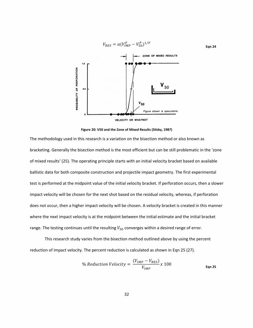
⁄ Eqn 24
Figure 20: V50 and the Zone of Mixed Results (Silsby, 1987)
The methodology used in this research is a variation on the bisection method or also known as
bracketing. Generally the bisection method is the most efficient but can be still problematic in the ‘zone
of mixed results’ (25). The operating principle starts with an initial velocity bracket based on available
ballistic data for both composite construction and projectile impact geometry. The first experimental
test is performed at the midpoint value of the initial velocity bracket. If perforation occurs, then a slower
impact velocity will be chosen for the next shot based on the residual velocity, whereas, if perforation
does not occur, then a higher impact velocity will be chosen. A velocity bracket is created in this manner
where the next impact velocity is at the midpoint between the initial estimate and the initial bracket
range. The testing continues until the resulting converges within a desired range of error.
This research study varies from the bisection method outlined above by using the percent
reduction of impact velocity. The percent reduction is calculated as shown in Eqn 25 (27).
Eqn 25

33
For each test matrix, a minimum of four velocity brackets were formed by five tests where at least one
of the shots had to have either no or partial perforation, another having as little change in impact
velocity as possible and the remaining shots covering at least 20% velocity brackets in between. A non-
perforating shot is considered to be close to the ballistic limit when a small pyramidal protrusion was
formed due to impact damage as shown in Figure 21, Figure 22, and Figure 23. By comparison the
pyramidal protrusion characteristic of a 77.2% velocity reduction is shown in Figure 24, Figure 25, and
Figure 26. The pyramidal protrusion is resultant of the {0/90}s construction panel. By characterizing the
energy absorption capabilities of the composite panels across a range of velocities, a better
understanding can be developed over a span of energy levels and the general correlation can be used to
develop the Finite Element model as demonstrated later.
Figure 21: Non-Perforating Pyramidal Protrusion, Back of Composite Panel

34
Figure 22: Close-up of Non-Penetrating Pyramidal Protrusion
Figure 23: Non-Penetrating Pyramidal Protrusion, Side View
Figure 24: 77.2% Velocity Reduction Pyramidal Protrusion, Back of Composite Panel

35
Figure 25: Close-up of 77.2% Velocity Reduction Pyramidal Protrusion
Figure 26: 77.2% Velocity Reduction Pyramidal Protrusion, Side View
Impact Testing The experimental testing was performed using the experimental accelerator highlighted in
Chapter 2: Experimental Setup. As has been mentioned earlier, the study of impact dynamics hinges on
the three conservation laws: conservation of mass, conservation of momentum, and conservation of
energy (6) (1). As such the experimental data collected during this study are the initial and residual mass
of the projectile and composite panel and the impact and residual velocity of the projectile.
During this research carbon fiber/epoxy {0/90}s Plain Weave composite panels were tested for
the impact response to a 316 stainless steel (SS) cylindrical projectile with a blunt impact face. A total of
four test cases were performed consisting of two panel thicknesses and three obliquity angles to the
normal of the composite panel plane. Obliquity induces bending into the target. As such, the wave

36
propagation in the composite panel is different to those normal to the target plane. For normal impacts,
a two dimensional stress state results whereas at obliquity, asymmetric bending waves form causing a
three dimensional stress state (2). So, by using different obliquity angles, a better understanding of the
performance characteristics of the test panel can be established.
Testing Results The data generated and collected from the impact testing is summarized in Figure 27. All four
test matrices are included for completeness. The velocities are normalized to the highest impact and
residual velocity within each test matrix. The Finite Element Simulations developed later is compared to
this data set.
Figure 27: Impact Test Data Summarization Matrix
Experimental Characterization of Composite Panels The experimental characterization of composite panels often utilizes a macro-mechanics
approach where the underlying assumptions are that the material is homogenous and any material
behavior due to the constituent materials can be represented as bulk properties (15). Due to the lay-up
pattern or construction of the composite panel, many composite materials exhibit orthotropic material
Ini. Wt. (g) Res. Wt. (g) Obliq. (°) Thick. (") Ini. Wt. (g) Res. Wt. (g) Vi Vres % Loss
1 1.55 1.55 0 0.18 149.45 148.95 0.82338 0.72427 35.35% 230 Yes
2 1.55 1.55 0 0.18 149.4 148.95 0.76293 0.56721 45.36% 155 Yes
3 1.55 1.55 0 0.18 150.75 150.75 0.63584 0.19708 77.22% 100.5 Yes
4 1.55 1.55 0 0.18 151.85 150.5 1 1 26.50% 500.4 Yes
5 1.55 1.55 0 0.085 71.95 71.95 0.51463 0 100.00% 100.3 No
6 1.55 1.55 0 0.085 72.95 72.75 1 1 20.15% 99.9 Yes
7 1.55 1.55 0 0.082 70.35 70.3 0.76307 0.60449 36.74% 90.5 Yes
8 1.55 1.55 0 0.087 72.95 72.75 0.94905 0.90645 23.73% 79.9 Yes
9 1.55 1.55 0 0.085 72 71.8 0.63473 0.28284 64.42% 40 Yes
10 1.55 1.55 30 0.087 73.95 73.75 0.59516 0.51622 24.59% 99.7 Yes
11 1.55 1.55 30 0.083 71.05 70.9 0.44793 0.33706 34.58% 95.2 Yes
12 1.55 1.55 30 0.085 73.35 73.15 0.4995 0.3851 32.98% 51 Yes
13 1.55 1.55 30 0.086 73.65 73.45 0.37848 0.06581 84.88% 50.2 Yes
14 1.55 1.55 30 0.084 71.75 71.55 1 1 13.06% 399.6 Yes
15 1.55 1.55 45 0.086 73.25 73.1 0.60167 0.46783 36.32% 70.6 Yes
16 1.55 1.55 45 0.084 71.45 71.25 0.45658 0.25073 55.03% 55.3 Yes
17 1.55 1.55 45 0.085 72.8 72.55 1 1 18.10% 398.8 Yes
18 1.55 1.55 45 0.084 71.95 71.65 0.86504 0.83643 20.81% 200.6 Yes
Penetr.
(Y/N)Test Case
Projectile Composite Panel Normalized Velocity Gun Press.
(psi)

37
behavior (15) (28). As such material properties must be developed in the three material directions and
planes which include Modulus of Elasticity, Modulus of Rigidity, Poisson’s Ratio, and tensile and
compressive strengths. As shown in Figure 28, the material directions we will be considering are in the 1,
2, and 3 directions. Since the construction is a {0/90}s Plain Weave laminate, we will consider the 1 and
2 directions to be in the fill and warp directions of the composite lamina.
Figure 28: Composite Material Directions in the Global Coordinate System (Adams et. al, 2003)
Tensile Testing
For obtaining the Elastic Modulus and Poisson Ratio in both the 1 and 2 material directions,
ASTM D3039 tensile test procedure was performed on the carbon fiber/epoxy panels. It was assumed
that the material behavior in both the 1 and 2 directions would be identical. As outlined in D3039,
sample preparation is critical in that the sample must be symmetric. Asymmetric sample geometry
could induce bending from asymmetric strains (28) (29). Also the sample must be free of any
imperfections due to the cutting process such as matrix cracking or delamination at the sample edges
which may initiate early sample failure (28) (29). Specific sample dimensions are outlined in the standard
in order for St. Venant’s principle to be applicable (28). In order to minimize the effect of compressive
stresses from the cross-head clamps, at each of the sample ends tabs are adhered as illustrated in Figure
29. Generally the tab material consists of a compliant material to reduce the stress concentration due to
the thickness discontinuity at the tab edge (28). It has been suggested that a good source of tab material
is commercially available glass-epoxy printed circuit board (PCB) as it is highly uniform in thickness with
very little warpage (28). The ASTM D3039 standard recommends that the cross-head rate be controlled

38
to a constant strain rate between ⁄ or a constant cross-head rate if constant
strain controls are not available (29). Cross-head speed is calculated by multiplying the recommended
strain rate by the distance between the sample tabs (29). A constant cross-head rate of ⁄
was used for this research.
Figure 29: Representation of Tabbed Sample (Adams et. al, 2003)
The testing was performed by Material Science Corporation (MSC). The test results are summarized in
Figure 30 for two different constructions; six samples were tested for each construction. The complete
test reports are located in Appendix B: Experimental Characterization Data.
Figure 30: D3039 Tensile Test Results Summary (MSC)
Tensile Testing: Off-Axis Shear
There are several available test standards available to establish shear modulus and strength
which include ASTM D5379 (Iosipescu Method), D4255 (Two-Rail Shear Method), D4255 (Three-Rail
Shear Method), and D3518 (45° Off-Axis Tensile Shear Method) (28). However, all of the
aforementioned methods require special test fixtures with the exception of D3518 Tensile Shear test
Stress (ksi) Modulus (msi) Poissons % Strain @ Failure
Avg 94.50 8.14 0.06 1.16
Std Dev 4.88 0.19 0.01 0.11
Avg 56.53 5.36 0.32 1.21
Std Dev 5.39 0.07 0.01 0.36 {0/90/45/-45}s
{0/90}s
D3039 Test Results

39
(30). As such, the D3518 standard is cheaper in that no expensive test fixture is required. As pointed out
by Adams et al, the tradeoff is that since the loading is not pure shear but also has normal in-plane
stresses, that the shear strength value obtained may be slightly lower than the true value (28). Adams et
al postulated that the actual difference may be small because of the softening behavior exhibited by
composite materials (28). The test procedure is essentially the same as that of D3039 with the only
difference in that the sample orientation is 45° off-axis similar to that depicted in Figure 28 with
.
For this research samples were not available to generate shear test data. As such the author
elected to approximate the shear properties using the data available for this research. There are several
micro-mechanics approaches to estimating the elastic properties based on the constituent material
properties and the fiber volume fraction of the composite material. However the approximation of the
shear modulus is often a lower-bound and requires an exact calculation of the fiber volume fraction
(15). Since data was available for the tensile test of a {0/90/45/-45}s quasi-isotropic construction, the
author proposes that the quasi-isotropic case could be used as an upper bound for the shear modulus
and strength of a {0/90}s construction composite. Figure 31 illustrates the aforementioned assumption
where the gray square represents the composite panel, the bidirectional arrows represent the
orientation of the laminates to the panel, the exterior arrows represent the loading direction for the
tensile test, and the dashed line rectangle represents the prepared sample and its relative orientation.
The desired test case for the {0/90}s D3518 test is represented in Figure 31 part a). The {0/90}s D3518
test can be considered identical to Figure 31 part b), {45/-45}s D3039 test, since the only difference is
the orientation that the prepared sample is cut relative to the finished panel. By extension, the
{0/90/45/-45}s D3039 test, Figure 31 part c), can be considered an upper bound since there are
additional layers compared to Figure 31 part b) and , as such, the shear modulus should be higher than
the desired case, {0/90}s D3518 test. As suggested by Adams et al for the D3518 test, the modulus of

40
elasticity and Poisson’s ratio will be treated as the apparent values and Eqn 26 was used to approximate
the shear modulus (28).
Eqn 26
Figure 31: {0/90}s D3518 Test, Approximation for Shear Modulus
Using Eqn 26 and the data from Figure 30 for the {0/90/45/-45}s construction yields Eqn 27.
Eqn 27
Compressive Testing
There are three main standard compressive tests in practice for composite panels which include
the ASTM D3410 (Shear Loading Method), Modified D695 (End Loading Method), and D6641 (Combined
Loading Compression Methods, CLC) (28). The D3410 utilizes a shear loading method in which the
shearing movement of the wedge grips compresses the test sample (28). Due to the size of the required
test fixture, a wide range of test sample sizes can be accommodated by the D3410 (28) (31). Some of the
drawbacks of the D3410 include large compressive forces at the wedge grips may crush the sample and
damage the surface of the sample due to grip roughness and the fixture required is very expensive and

41
large (28). Another method is by end load application in the Modified D695 test. The primary
disadvantage is that some level of buckling may occur (28). In addition the test fixture may cause a
redundant load path which can lead to higher values for the compressive strength and modulus (28).
The D6641 standard uses a combination of shear and end loading. The shear loading is achieved through
the clamping blocks and denotes that compression is provided by the blocks (28). The end loading is
present since the ends of the sample are flush with block ends as shown in Figure 32 (28). The amount
of shear loading is controlled in the amount of clamping force used to retain the sample (28). This
minimizes the possibility of crushing the sample as compared to the D3410 (28). Given the benefits
outlined of the D6641 test and the availability of the test fixture, MSC performed the compression
testing. The data is summarized in Figure 34 and the test reports are included in Appendix B:
Experimental Characterization Data.
Figure 32: Sketch of CLC test fixture (Adams et al 2003)

42
Figure 33: CLC test fixture (Adams et al 2003)
Figure 34: D6641 Compressive Test Results Summary (MSC)
Finite Element Model Overview
Model Geometry and Mesh Generation
In the simulations both the projectile and the composite panel consist of 8 node ‘brick’ solid
elements with a single integration point to reduce the simulation runtimes. Each ply of the composite
panel is represented as a separate part. In order to avoid the creation of tetrahedral elements, a shell
surface was created to generate four node rectangular elements (Q4) as shown in Figure 35. On each of
the twelve lines creating the four quadrants of the sample, an initial number of 30 nodes per line were
used as the basis to generate the quadrilateral mesh. The duplicate nodes on the interior lines were
consolidated to prevent massless, duplicate nodes. Since the loading of an impact event is highly
localized, a much finer mesh is employed surrounding the impact area and gradually becomes more
Stress (ksi) Modulus (msi)
Avg 75.86 7.62
Std Dev 3.49 0.24
Avg 53.10 5.19
Std Dev 1.91 0.08
D6641 Test Results
{0/90}s
{0/90/45/-45}s

43
coarse out towards the free edges of the sample (32). As such, a bias of 5 towards the center of the
composite panel was employed. Each layer was created by performing an element generation sweep
normal to the composite panel plane of one element thick. The process was repeated for each
subsequent layer in the composite panel.
Figure 35: Q4 Shell Element Plane Used to Generate Solid Elements
The clamped perimeter boundary condition of the composite panel holder is shown in Figure 36.
The composite test samples measures 6” H x 6” W while the inner square opening of the panel holder
measures 5” H x 5” W. In the impact testing the samples were centered evenly with respect to the
holder and thus 0.5” of clamping surface was present surrounding the composite panel perimeter. The
panel holder was considered to be much more rigid than the composite panel to where and
deformation or displacement of the holder due to the impact forces was considered negligible. In
consideration of the aforementioned assumption, the 0.5” perimeter of the composite panel is
considered constrained in the X, Y, and Z degrees of freedom as highlighted in Figure 37 by the white
points.

44
The cylindrical projectile was created using a 3-D computer-aided drafting program. After
importing the geometry data a similar process as outlined for the composite panel mesh generation was
followed. A shell element plane was created at the flat base of the cylinder and then mesh generation
sweep was performed into the volume of the projectile. As can be seen from examination of Figure 37
and Figure 38, the mesh of the projectile is much denser than the composite panel. Zukas recommends
that a finer mesh be used in the projectile in order to provide better engagement for the contact
elements (32).
Figure 36: Representation of Test Sample Holder with Composite Panel (AMRDEC, 2010)
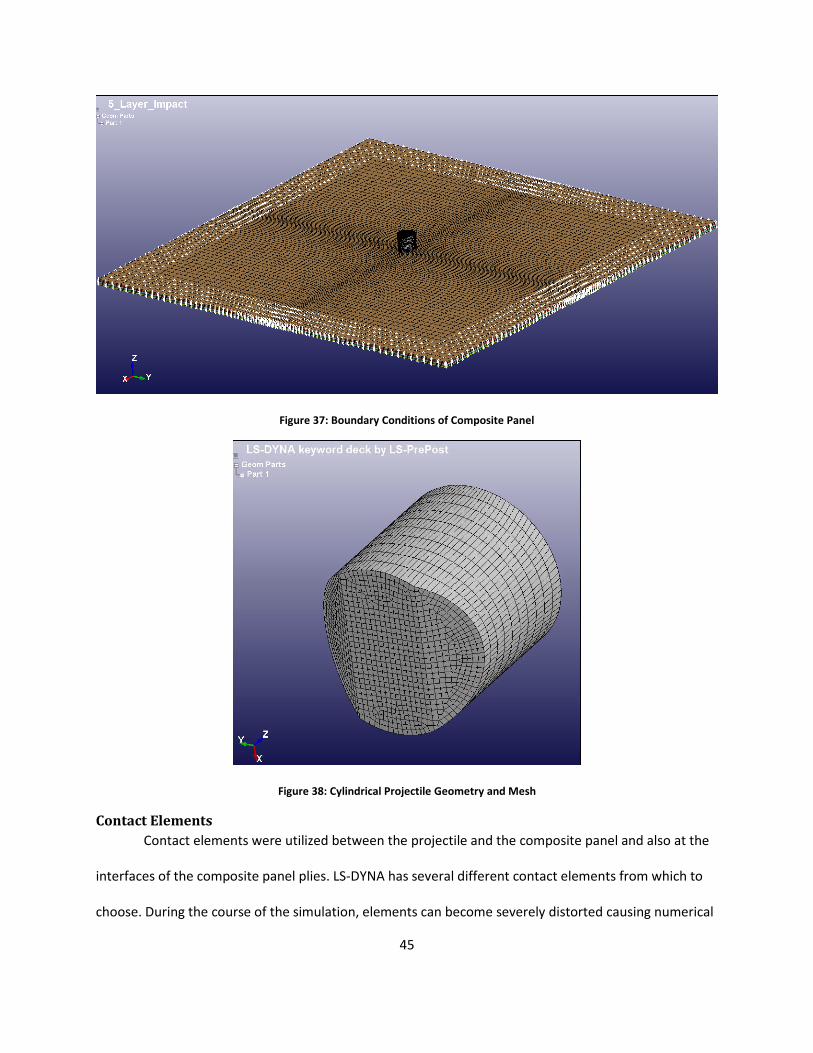
45
Figure 37: Boundary Conditions of Composite Panel
Figure 38: Cylindrical Projectile Geometry and Mesh
Contact Elements
Contact elements were utilized between the projectile and the composite panel and also at the
interfaces of the composite panel plies. LS-DYNA has several different contact elements from which to
choose. During the course of the simulation, elements can become severely distorted causing numerical

46
instabilities. One technique to alleviate the problem of overly distorted elements is deletion or erosion
of elements once specific criteria are met. In order to allow for erosion due to impact of the projectile,
CONTACT_ERODING_SURFACE_TO_SURFACE was added between the projectile and the composite
panel. The default values were used as shown in Figure 39. Since the plies of the composite panel are
treated as separated parts in this research, contact elements are required at the ply interfaces and
CONTACT_AUTOMATIC_SURFACE_TO_SURFACE_TIEBREAK was used. The delamination criteria selected
is shown in Eqn 28 where and are the normal and shear stresses and NFLS and SFLS are the
normal and shear failure stresses, respectively (14). As shown in Figure 40, Option 2 was selected so that
nodes that are initially in contact remained tied, which prohibits tangential motion, until failure occurs
(14). The NFLS and SFLS values were approximated based on the study of S-2 Glass beams by Sevkat et al
(21). Please note in Figure 40 the properties listed below are using the base units of kilograms, meters,
and seconds, thus the stresses are listed in Pascals. This unit convention is used throughout the finite
element model.
(
| |
)
(| |
)
Eqn 28
Figure 39: Projectile/Composite Panel Contact Element

47
Figure 40: Composite Panel Interface Contact Element
Projectile Material Model
The projectile is manufactured from 316 SS. In this model, the 316 SS is considered to be a linear
elastic, plastic isotropic material and thus the MAT_PLASTIC_KINEMATIC material model was used.
Additionally, the model can apply different levels of isotropic or kinematic hardening through the Beta
parameter where Beta=0 is pure kinematic hardening and Beta=1 is pure isotropic hardening as is shown
in Figure 42. Generally, kinematic loading is better suited for cyclic loading conditions such as fatigue
simulations whereas in the case of impact a softening effect is created. From experimental observation,
premature element erosion in the projectile will occur due to interaction with the contact elements if
kinematic hardening is utilized. As such pure isotropic hardening was selected to eliminate any non-
observed material erosion in the projectile.
Figure 41: MAT_PLASTIC_KINEMATIC Projectile Material Model

48
Figure 42: MAT_PLASTIC_KINEMATIC Hardening Theory
Projectile Model Parameter Definitions
The mass density is designated as RO. E is the elastic modulus. PR is Poisson’s ratio. SIGY
denotes the yield stress. ETAN represents the bilinear elastic behavior of steel and is the slope of the
stress/strain curve as illustrated in Figure 42. FS is the failure strain of the steel.
Composite Material Model
As explained earlier due to the composite panel construction the material behavior will be
treated as orthotropic. Damage in composites consists of different fiber and matrix failure modes which
include fiber fracture, fiber-matrix separation, fiber pull-out, epoxy matrix cracks, and delamination (9).
Composite panels also exhibit softening behavior that arises after the initiation of damage (33). In order
to accurately model a dynamic event such as an impact penetration and perforation, the
aforementioned material behavior, in addition to strain rate effects, will need to be considered. There
are several composite material models available to use in LS-DYNA but the
MAT_COMPOSITE_DMG_MSC or MAT_162 material model is the only comprehensive model that takes
into account all of the material behavior effects mentioned (14). MAT_162 is an anisotropic composite

49
material model with progressive damage developed by Material Sciences Corporation (MSC) (14). The
failure criteria is based on Hashin’s failure criteria for unidirectional laminates but has been generalized
for application to plain weave laminates as well (14) (34). The damage model is based on the approach
developed by Matzenmiller, Lubliner, and Taylor or sometimes referred to as the MLT damage model
(35). A treatment of the components to the MAT_162 material model will be outlined in the following
sections that are shown in Figure 43.
Figure 43: MAT_COMPOSITE_DMG_MSC Composite Panel Material Parameters
Material Model Coordinates and Laminate Construction
LS-DYNA allows for the user to define the material coordinate system with respect to the global
coordinate system. There are several different options available for suitability to a wide range of part
geometries. Since the composite panel geometry is rectangular by both geometry and in construction,
AOPT=2 was selected. As illustrated in Figure 44, the user defines both vectors A and D and LS-DYNA will
calculate vectors B and C. A1, A2, A3 and D1, D2, D3 are the global x, y, z components of vectors A and D
respectively. For this research A1=1 and D2=1 in which vectors B and D both equal and C equals . As
such material directions A and B are in the fiber directions , fill and warp, and C is in the thickness
direction. Since the layers of the composite panel are plain weave, AMODEL =2 was selected.

50
AMODEL=2 enable certain failure criteria that are associated with plain weave laminates in the material
model.
Figure 44: Definition of AOPT=2 Material Coordinates (Hayduke, 2010)
Elastic Properties
The elastic properties follow the coordinate convention previously defined. EA, EB, and EC are
the elastic moduli in the A, B, and C material directions respectively. PRBA, PRCA, PRCB are the Poisson’s
ratio in the B-A, C-A, and C-B material planes. The elastic moduli and Poisson’s ratios are taken from the
results of the ASTM testing summarized earlier. GAB, GBC, and GCA are the shear moduli in the A-B, B-C,
and C-A material planes. As mentioned before the shear moduli were developed by the approximating
the value given in Eqn 27.
Strength Properties
SAT and SAC are the tensile and compressive strengths in the A direction. SBT and SBC are the
tensile and compressive strengths in the B direction. The tensile and compressive strengths in the A and
B fiber directions are taken from the ASTM testing results. SAB, SBC, and SCA are defined as matrix
mode shear strengths in the A-B, B-C, and C-A material planes. The matrix mode shear strengths were
approximated by using the D3039 strength results for the quasi-isotropic test case.
SCT and SFC are the tensile (interlaminar) and compressive (crush) strengths in the C direction
(14) (36). SFS is defined as the fiber mode shear (punch shear) strength (14) (36). SCT, SFC, and SFS were
approximated based on a S2-glass model as no experimental data was available (36). As noted by Xiao et

51
al determining SCT is difficult as different methods will yield varying values (36). Material Sciences
Corporation has developed a specialized Laterally Constrained Compressive Testing Fixture to determine
SFC and SFS but no data for carbon fiber laminates are currently available (36).
SFFC is defined as the scale factor for residual compressive strength (14). SFFC=0.3 was used
based on a S-2 glass material model (36). S_DELM is the shear stress concentration at the free edges.
S_DELM=1.6 was used in the research from a unidirectional carbon fiber model developed by MSC (33).
Erosion Parameters
MAT_162 also allows for element erosion of the composite panel. The erosion parameters:
E_LIMT, ECRSH, and EEXPN are based on the maximum strain limit and volume expansion and
compression for the element respectively. Conservative values were selected in order to prevent
premature element erosion in the model simulation and were based on the model by Xiao et al (36).
Strain Rate Coefficients
MAT_162 also requires four strain rate coefficients: CERATE1, CERATE2, CERATE3, and CERATE4
for the strength properties, axial moduli, shear moduli, and transverse moduli respectively. The strain
rate coefficients can be developed using the Split Hopkinson Pressure Bar tests (33). The strain rate
coefficients were approximated by using the S-2 glass material model values since no experimental data
was available for this research.
The strain rate dependent behavior of the composite panel for the strength properties { }
and elastic moduli { } are represented in Eqn 29 and Eqn 31 respectively (14) (33). { } and { } are
the strength and elastic moduli at the reference strain rate (14) .
{ } { } (
{ }
)
Eqn 29
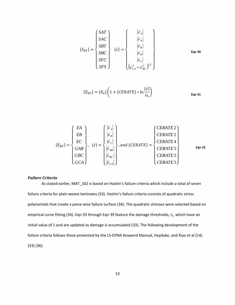
52
{ }
{
SFS
SFC
SBC
SBT
SAC
SAT
}
{ }
{
2122
BCCA
C
B
B
A
A
}
Eqn 30
{ } { } ( { }
{ }
)
Eqn 31
{ }
{
GCA
GBC
GAB
EC
EB
EA
}
{ }
{
CA
BC
AB
C
B
A
}
{ }
{
3
3
3
4
2
2
CERATE
CERATE
CERATE
CERATE
CERATE
CERATE
}
Eqn 32
Failure Criteria
As stated earlier, MAT_162 is based on Hashin’s failure criteria which include a total of seven
failure criteria for plain weave laminates (33). Hashin’s failure criteria consists of quadratic stress
polynomials that create a piece-wise failure surface (34). The quadratic stresses were selected based on
empirical curve fitting (34). Eqn 33 through Eqn 39 feature the damage thresholds, , which have an
initial value of 1 and are updated as damage is accumulated (33). The following development of the
failure criteria follows those presented by the LS-DYNA Keyword Manual, Hayduke, and Xiao et al (14)
(33) (36).

53
Fiber Tensile/Shear Failure Modes
Eqn 33 and Eqn 34 represent the fiber tensile and shear failure modes in both the A and B material
directions respectively. The damage is represented by the quadratic interaction between the axial and
through thickness shear strains (14).
(
)
(
)
Eqn 33
(
)
(
)
Eqn 34
Fiber Compressive Failure Modes
Eqn 35 and Eqn 36 represent the fiber compressive failure modes in the A and B directions. It is based
on the assumption that the damage is given by the maximum strain criterion (14).
(
)
⟨ ⟩
Eqn 35
(
)
⟨ ⟩
Eqn 36
Fiber Crush Failure Mode
Eqn 37 models the crush failure due to compressive forces in the thickness direction (14).
(
)
Eqn 37
Fiber In-Plane Shear Failure Mode
Eqn 38 models the damage that can occur in a plain weave due to in-plane shear stress excluding fiber
fracture (14). This damage can include fiber pull-out (9).
(
)
Eqn 38

54
Delamination Failure Mode
Eqn 39 relates the through thickness normal and shear stress to the through thickness strength and the
interlaminar shear strengths in the through thickness planes B-C and C-A. The relationship also includes
the effect of stress concentrations on the free ends by using the SDELM parameter. According to the
Mohr-Coulomb theory, the interlaminar shear strengths are set to increase under compression and
decrease under tension through the inclusion of from Eqn 40 (36).
{(
)
(
)
(
)
}
Eqn 39
Eqn 40
Damage Model and Parameters
MAT_162 adopts the MLT damage approach by introducing damage variables where j=1,…,6
to model the initiation and progress of damage leading to composite softening (33). The compliance
matrix shown in Eqn 20 now takes the form of Eqn 41. The damage variables are applied to the stiffness
components for both extension and shear responses. The damage parameters, AM1, AM2, AM3, and
AM4, can range from values of 0 to 100. Generally, numerically lower AM values leads to more ductile
material response whereas higher values lead to a more brittle material response (36).

55
[ ]
[
CA
BC
AB
CB
BC
A
AC
C
CB
BA
AB
C
CA
B
BA
A
G
G
G
EEE
EEE
EEE
6
5
4
3
2
1
1
100000
01
10000
001
1000
0001
1
0001
1
0001
1
]
Eqn 41
As proposed by Matzenmiller et al, the growth rate of the damage variables, , are dictated by Eqn 42
where , are the scalar damage functions and are defined in Eqn 43 (35). Eqn 43 defines the damage
coupling functions, , where AM is the damage parameter and is the damage threshold.
∑
Eqn 42
( )
Eqn 43
The damage coupling functions, , for the plain weave model are listed in Eqn 44 (36).
[ ]
[
10111
00100
11111
10100
00100
00111
]
Eqn 44
The preceding development leads to Eqn 45 which represents the reduced elastic and shear moduli,
and , where and represent the initial elastic and shear moduli (14) (36).
, Eqn 45

56
Finite Element Simulations As noted earlier, composites exhibit a softening behavior once damage has initiated. It is
difficult to experimentally develop the damage parameter values as different testing methodologies can
yield a wide range of values (36). A parametric study was performed by Xiao et al for a quasi-static
punch-shear test to develop the damage parameters on the basis that the material behavior in response
to punch-shear is similar to that of impact (36). In this research, a similar approach is taken to develop
the damage softening parameters. A parametric study was performed to compare the predicted finite
element model response with the experimental residual velocity over a range of impact velocities for a
single test matrix. The damage parameters were changed systematically to determine the effects each
of the parameters had on the model behavior. The anticipated advantages to analyzing the FE model
response over a range of impact velocities as opposed to establishing the singular value is that:
1) a more accurate model can be developed for the energy absorption capabilities of the
composite material
2) a better understanding can be gained of the composite materials’ damage mechanics.
The test matrix was developed using a Design of Experiments methodology where three values
were selected for each damage parameter: a low, a mid-range, and a high value. The mid-range values
were treated as the baseline values. The baseline values of AM1=AM2=AM3=AM4=4 were selected
based on literature recommendations (33). A single damage parameter was changed at a time to avoid
any possible interaction effects between the parameters. The only exception to the interaction effects
restriction are AM1 and AM2 since these parameters are the fiber damage in the material A and B
material directions and as such were changed at the same time with the requirement of being equal.
Since each test case actually consists of several impact tests, a FE simulation was ran for each
data point to create the response over the impact velocity range. From the Recht-Ipson formula, a
logarithmic relationship between residual and impact velocity is expected but since such a small portion

57
of the curve is being reviewed these can be approximated to be linear or bi-linear. As such the assumed
residual and impact velocity relationship is approximated to be either a linear or bi-linear relationship
throughout the parametric study. Based on FE model predictions a qualitative curve-fitting evaluation
checking for linearity was employed to select the calibrated material properties. A linear regression was
used in all cases and comparison of the , coefficient of determination, was used for cases that could
not be evaluated solely on a qualitative basis. Once the calibrated damage parameters were established,
the material model was applied to the other three test cases where obliquity angle was changed and
also panel thickness was increased. By applying the FE model to different loading conditions and sample
dimensions, the validity of the FE model can be evaluated for conditions outside the initial bounds for
which the model was developed and give an indication of model robustness.
Parametric Study: 5 Layer Panel, 0° Obliquity
Baseline Comparison
The test matrix selected for model calibration is the 5 layer composite panel, 0° obliquity and
was selected on the basis that the wave propagation would be symmetric. As mentioned before, the
baseline values were selected based on literature recommendations. An initial evaluation of the baseline
was performed to confirm a linear relationship between the Residual and Impact velocities. Figure 45
summarizes the results and Figure 46 documents the parameters used. As can be seen in the plot,
Iteration 4 using the baseline values of 4 exhibits the most linear relationship and will be a good starting
point for calibration. In Figure 46 the green shading denotes the variables being considered. The green
shading convention will used throughout the section.

58
Figure 45: Damage Parameters Baseline Comparison
Figure 46: Baseline Variable Matrix
AM1, AM2 Fiber Softening Effects
The AM1 and AM2 are the fiber softening parameters in the A and B material directions (14). As
Figure 47 shows increasing (Iteration 11) and decreasing (Iteration 12) AM1 and AM2 does not provide a
better fit to the data than the baseline (Iteration 4). The ill fit is most apparent at the data point of
62.5% relative residual velocity for Iteration 11 although a better fit is obtained at 72.5% relative
residual velocity. Figure 48 shows the parameters used.
Iteration Iteration 4 Iteration 13 Iteration 14
Layers/Thickness 5/0.0848" 5/0.0848" 5/0.0848"
Obliquity 0 0 0
Mesh 30 30 30
AM1 (Fiber A dir) 4 2 6
AM2 (Fiber B dir) 4 2 6
AM3 (PunchS/Fiber Shear) 4 2 6
AM4 (Delamination) 4 2 6

59
Figure 47: AM1, AM2 Fiber Softening Effects Comparison
Figure 48: Fiber Softening Variable Matrix
AM3, Fiber Crush/Punch Shear Effects
AM3 is the fiber crush and punch shear parameter (14). AM3 showed the strongest effect on the
overall model response of all of the damage parameters. Iteration 7 (increased AM3) and Iteration 8
(decreased AM3) loses linearity and are most severely affected at 72.5% relative residual velocity as
shown in Figure 49. As such fiber crush and punch shear effects are critical as these failure modes have
the largest effect on the composite materials energy absorption capability. Figure 50 documents the
parameters used.
Iteration Iteration 4 Iteration 11 Iteration 12
Layers/Thickness 5/0.0848" 5/0.0848" 5/0.0848"
Obliquity 0 0 0
Mesh 30 30 30
AM1 (Fiber A dir) 4 6 2
AM2 (Fiber B dir) 4 6 2
AM3 (PunchS/Fiber Shear) 4 4 4
AM4 (Delamination) 4 4 4

60
Figure 49: AM3 Fiber Crush, Punch Shear Comparison
Figure 50: Fiber Crush, Punch Shear Variable Matrix
AM4, Matrix/Delamination Effects
AM4 is defined as the matrix and delamination parameter (14). AM4 had the least dramatic
effect on the model response. However by increasing AM4 (Iteration 9) a better overall fit was obtained
as shown in Figure 51 and an improvement in the linearity as evidenced by a slightly higher regression
value for Iteration 7 versus for Iteration 4 and for Iteration 10.
Figure 52 documents the parameter values used.
Iteration Iteration 4 Iteration 7 Iteration 8
Layers/Thickness 5/0.0848" 5/0.0848" 5/0.0848"
Obliquity 0 0 0
Mesh 30 30 30
AM1 (Fiber A dir) 4 4 4
AM2 (Fiber B dir) 4 4 4
AM3 (PunchS/Fiber Shear) 4 6 2
AM4 (Delamination) 4 4 4
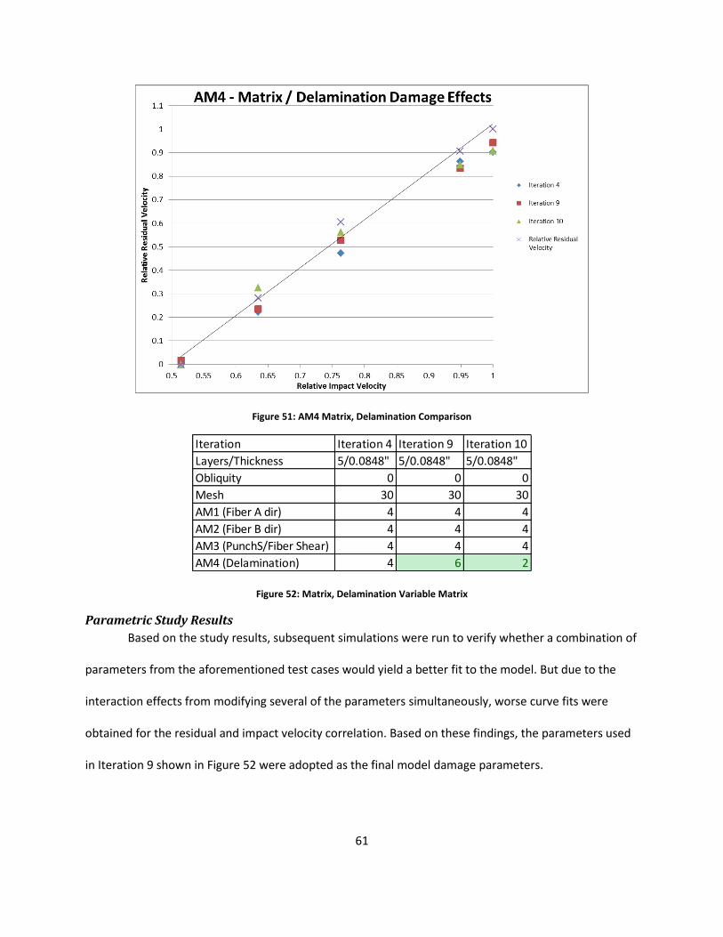
61
Figure 51: AM4 Matrix, Delamination Comparison
Figure 52: Matrix, Delamination Variable Matrix
Parametric Study Results
Based on the study results, subsequent simulations were run to verify whether a combination of
parameters from the aforementioned test cases would yield a better fit to the model. But due to the
interaction effects from modifying several of the parameters simultaneously, worse curve fits were
obtained for the residual and impact velocity correlation. Based on these findings, the parameters used
in Iteration 9 shown in Figure 52 were adopted as the final model damage parameters.
Iteration Iteration 4 Iteration 9 Iteration 10
Layers/Thickness 5/0.0848" 5/0.0848" 5/0.0848"
Obliquity 0 0 0
Mesh 30 30 30
AM1 (Fiber A dir) 4 4 4
AM2 (Fiber B dir) 4 4 4
AM3 (PunchS/Fiber Shear) 4 4 4
AM4 (Delamination) 4 6 2

62
Mesh Comparison
As mentioned in an earlier section the mesh was created with a total of 30 nodes per each
quadrant edge of the composite panel with biasing of 5. In order to verify whether the Finite Element
model still had a dependence on the mesh, a finer mesh was created with which to compare. The nodes
per each quadrant edge was increased to 40 nodes while maintaining a bias of 5 to allow for the finer
mesh in the center of the composite panel as shown in Figure 35.
In Figure 53 the comparison between the 30 node per edge case (Iteration 9) and the 40 node
per edge case (Iteration 18) is plotted. It is evident that at low percent reductions in speed (20%) and
around the ballistic limit almost no change in the predicted residual velocity occurred. But there was a
greater change at the midrange percent reductions. Since there was negligible change at the ballistic
limit, the 40 node per edge case was adopted as the mesh used throughout the remainder of the
research.
Figure 53: Mesh Comparison

63
Figure 54: Mesh Comparison Variable Matrix
Resulting 5 Layer 0° Obliquity Model Comparison to Experimental Data
The resulting Finite Element model results are compared to the experimental data as shown in
Figure 55. Linear regression curve fits were applied to each of the data sets to compare the overall fit
and are color-matched in Figure 55. The two fits are almost identical but have slightly different slopes
but both agree on the prediction of the ballistic limit 0% relative residual velocity. As such there is good
agreement between the Finite Element model and the experimental data.
Figure 55: 5 Layer Composite 0° Obliquity Model Results
Iteration Iteration 9 Iteration 18
Layers/Thickness 5/0.0848" 5/0.0848"
Obliquity 0 0
Mesh (Nodes/Edge) 30 40
AM1 4 4
AM2 4 4
AM3 4 4
AM4 6 6

64
5 Layer Composite Panel, 30° Obliquity
The model for the preceding 0° obliquity case was modified to verify model accuracy for the 30°
obliquity case. As is evidenced from the plot shown in Figure 56, a bi-linear response was obtained in
this test case. Again a good agreement between the FE model and the experimental data was attained
throughout the velocity range. Since there was a large velocity span in the experimental data, three
interpolation points were added which also exhibit good agreement to the overall residual versus
impact velocity correlation.
Figure 56: 5 Layer Composite 30° Obliquity Model Results
10 Layer Composite Panel, 0° Obliquity
A new model was created to simulate the 10 layer thick 0° obliquity test case. The mesh density
and softening parameters are the same as Iteration 18 in Figure 54. As is shown in Figure 57, the FE
model prediction does not as closely match the experimental data compared to the test cases where the
model was created with the same thickness. Based on the findings, it is evident that the damage
mechanics are different for thicker panels as compared to thinner panels. It is suspected that the fiber
crush and punch shear damage effects may play a larger role in the thicker case.

65
Figure 57: 10 Layer Composite 0° Obliquity Model Results
Qualitative Model Response The finite element simulations involved with both the parametric study and the extrapolated
models created to verify model robustness focused primarily on the development of the ballistic limit
velocity to establish the energy absorption capabilities of the composite panels. However no attention
was paid to other model response characteristics such as the level of deflection of the composite panel,
the propagation of damage, or the damage incurred. Several test cases will now be reviewed for the
aforementioned qualitative model responses.
5 Layer 0° Obliquity, No Perforation – Test Case 5
The video stills shown in Figure 61 are from the 5 layer, 0° obliquity test case 5 as shown in
Figure 27. The stills show that the projectile does not perforate and ricochets. There is no creation of a
particle field from the impact and no measureable difference in mass. The damage incurred from the
actual panel is shown in Figure 58, Figure 59, and Figure 60 where little damage is incurred in the test
panel. In the LS-DYNA postprocessor, the model predicts a greater level of penetration and damage

66
incurred than observed experimentally. This is readily apparent in Figure 62 where the postprocessor
video stills show penetration that can be classified as a partial perforation. The LS-DYNA velocity plot in
Figure 63 shows that the projectile is bouncing back going from an impact velocity of negative 100 to
positive 14.80 meters per second in the global Z direction. Also evident from Figure 61 is that there is
relatively little deflection of the panel. Although no measurement system was in place to directly
measure the deflection, the target frame thickness of 6.35 mm can be used as a reference. Since the
panel deflection is not seen in the video stills, the deflection is expected to be less than 6.35 mm. In
Figure 64 and Figure 65 the nodes used to measure the amount of deflection and the deflection over
time are shown respectively. From the plot, maximum deflection is approximately 10 mm for the three
nodes selected which exceeds the experimental observation.
Figure 58: Test Case 5 Damage, Front View
Figure 59: Test Case 5 Damage Close Up

67
Figure 60: Test Case 5 Side View

68
Figure 61: Test Case 5 Video Stills, No Perforation, Projectile Ricochets

69
Figure 62: LS-DYNA Video Stills, Side View - Test Case 5
Figure 63: LS-DYNA Projectile Velocity Plot – Test Case 5

70
Figure 64: Measurement Nodes for Deflection, Test Case 5
Figure 65: Test Case 5 Deflection
5 Layer 0° Obliquity, 20% Velocity Reduction – Test Case 6
The video stills shown in Figure 68 are for the 5 Layer 0° obliquity test case 6 which resulted in a
20.15% velocity reduction. As shown in the video stills, a large particle field results from the impact. The
resulting damage can be examined in Figure 66 and Figure 67. From Figure 67 evidence of fiber fracture,
matrix cracking, and delamination are apparent but the propagation of damage is not obvious. After
reviewing the LS-DYNA simulation video stills in Figure 69, fiber fracture occurred first then matrix

71
cracking and delamination. Also the damage incurred on the panel is qualitatively similar to that
observed in Figure 67. However no particle field is created in the LS-DYNA video stills. In addition, less
delamination occurs in the LS-DYNA model than that observed experimentally. This suggests that the
delamination failure parameters in the contact elements between the layers may be approximated too
high a value.
Figure 66: Test Case 6 Damage
Figure 67: Test Case 6 Damage Close Up

72
Figure 68: Test Case 6 Video Stills, 20.15% Velocity Reduction

73
Figure 69: LS-DYNA Video Stills, Side and Back Views - Test Case 6

74
Conclusion A successful Finite Element model simulating the ballistic impact of a composite panel was
created. The model was able to model the energy absorption capabilities of the composite panel by
accurately predicting the residual projectile velocity over a range of impact velocities. The parametric
study allowed for calibration of the material model damage softening parameters using a single test
matrix. Extrapolation beyond the original boundaries of the parametric study demonstrated that once
the material model is calibrated, the model is able to predict the residual velocity for different projectile
trajectory obliquities and to some extent different panel thicknesses. The model agreement to
experimental data for the increased panel thickness case was lower. It is expected that due to the extra
thickness, the damage mechanics varies from that of the thinner panel.
Although the residual velocity predictions were in good agreement, other model responses did
not exactly match the observed experimental behavior. The incurred level of damage and the damage
characteristics did not always match. None of the simulations were able to reproduce the pyramidal
protrusion shown in Figure 24. The author suspects that the model is overly elastic and thus is not able
to reproduce the plastic behavior evident of the pyramidal protrusion. This suspicion is confirmed due to
the higher than observed level of deflection summarized by Figure 65. The overly elastic behavior is
likely due to the fact that the shear moduli and strengths were estimated based on the quasi-isotropic
construction composite. The model also over-predicted the level of damage in test case 5 with no
perforation. The damage over-prediction is likely resultant of both the contact and MAT_162 material
model’s erosion parameters.
Based on the findings outlined, several recommendations can be made regarding future study.
The Finite Element model used in the research utilized a macro-scale modeling technique where the
bulk properties are represented through the material model and the actual composite geometry is
simplified. As such, extensive material characterization is needed to develop a Finite Element model

75
and, as was the case with this research, characterization data may not be readily available to propagate
the MAT_162 material model. In order to reduce the amount of experimental characterization needed,
meso-scale modeling representation can be used where more sophisticated geometries are utilized.
Meso-scale modeling includes the weave geometry of the yarns so that effects caused by behavior such
as the friction between yarns in the weave or tension in the yarns due to crimping caused by the weave
pattern. Also further study is needed to better develop the contact elements between the composite
layers to simulate delamination. The amount of delamination resulting in the simulations was less than
experimentally observed which could also be linked to the resulting increase in the delamination
softening parameter, AM4, for the MAT_162 material model.

76
References 1. Nicholas, Theodore and Recht, Rodney F. Introduction to Impact Phenomena. [book auth.] Jonas A.
Zukas. High Velocity Impact Dynamics. s.l. : John Wiley & Sons, Inc., 1990.
2. Zukas, Jonas A. Introduction to Penetration Mechanics. High Velocity Impact Dynamics. s.l. : John
Wiley & Sons, Inc., 1990.
3. Wright, Thomas, W. A Survey Of Penetration Mechanics For Long Rods. Aberdeen Proving Ground,
Maryland : Ballistic Research Laboratory, 1983. ARBRL-TR-02496.
4. John Hopkins University. Project THOR, The Resistance of Various Metallic Materials to Perforation by
Steel Fragments; Empirical Relationships for Fragment Residual Velocity and Residual Weight. s.l. :
Ballistics Analytics Laboratory, 1961. Technical Report No. 47.
5. —. Project THOR, The Resistance of Various Non-Metallic Materials to Perforation by Steel Fragments;
Empirical Relationships for Fragment Residual Velocity and Residual Weight. s.l. : Ballistic Analytics
Laboratory, 1963. Technical Report No.51.
6. Recht, Rodney F. High Velocity Impact Dynamics: Analytical Modeling of Plate Penetration Dynamics.
[book auth.] Jonas A. Zukas. High Velocity Impact Dynamics. s.l. : John Wiley & Sons, Inc., 1990.
7. On the Lambert-Jonas approximation for ballistic impact. Ben-Dor, G., Dubinsky, A. and Elperin, T. 29,
s.l. : Elsevier Science Ltd., 2002, Vol. Mechanics Research Communications.
8. Cook, Robert D., et al., et al. Concepts And Applications Of Finite Element Analysis. s.l. : John Wiley &
Sons. Inc., 2002. ISBN: 0-471-35605-0.
9. Ochoa, O. O. and Reddy, J. N. Finite Element Analysis of Composite Laminates. s.l. : Kluwer Academic
Publishers, 1992. ISBN: 0-7923-1125-6.
10. (LSTC), Livermore Software Technology Corporation. LS-DYNA Theory Manual. s.l. : (LSTC),
Livermore Software Technology Corporation, 2006.
11. Tabiei, Ala. LS-DYNA Implicit Notes. s.l. : Livermore Software Technology Corporation (LSTC), 2003.
12. Mohan, Pradeep. Vehicle Crashworthiness, CE264 - Implicit Analysis Lecture. George Washington
University. [Online] 2010. [Cited: November 10, 2010.]
http://crash.ncac.gwu.edu/pradeep/CE264/lecture_5/lecture_5.pdf.
13. Finite-element modeling of the ballistic impact of fabric armor. Lim, C.T., Shim, V.P.W. and Ng, Y.H.
s.l. : International Journal Of Impact Engineering, 2002, Vol. 28.
14. (LSTC), Livermore Software Technology Corporation. LS-DYNA Keyword User's Manual Version 971.
s.l. : (LSTC), Livermore Software Technology Corporation, 2007.

77
15. Jones, Robert M. Mechanics Of Composite Materials. s.l. : Taylor & Francis, 1999. ISBN: 1-56032-
712-X.
16. Stilp, A. J. and Hohler, V. Experimental Methods for Terminal Ballistics and Impact Physics. [book
auth.] Jonas A. Zukas. High Velocity Impact Dynamics. s.l. : John Wiley & Sons, Inc., 1990, pp. 515-592.
17. Seigel, Arnold E. The Theory of High Speed Guns. s.l. : United States Naval Ordinance Laboratory,
1965.
18. Fox, Robert W. and McDonald, Alan T. Introduction to Fluid Mechanics. s.l. : John Wiley & Sons, Inc.,
1998. ISBN 0-471-12464-8.
19. A combined experimental and numerical approach to study ballistic response of S2-glass
fiber/toughened epoxy composite beams. Sevkat, E., et al., et al. 2009, Composites Science and
Technology.
20. NAC Image Technology. NAC HotShot 512sc User's Manual. 2010.
21. Estimation Of Ballistic Limit Velocities For Woven Composite Beams. Sevkat, E., et al., et al. s.l. :
ASME, 2009. ASME International Mechanical Engineering Congress & Exposition.
22. A new membrane model for the ballistic impact response and V50 performance of multi-ply fibrous
systems. Phoenix, S. Leigh and Porwal, Pankaj K. 40, s.l. : Elsevier Ltd., 2003, Vol. International Journal
of Solids and Structures.
23. Ballistic Perforation Dynamics. Recht, R.F. and Ipson, T.W. s.l. : Journal of Applied Mechanics, 1963,
Vol. 30.
24. Lambert, J. P. and Jonas, G. H. Towards Standardization in Terminal Ballistics Testing: Velocity
Represention. Aberdeen Proving Grounds, MD : Ballistic Research Laboratories, 1975.
25. Ferriter, E. Andrew, McCulloh, Ian A. and DeRosset, William. Techniques Used to Estimate Limit
Velocity in Ballistics Testing with Small Sample Size. s.l. : U.S. Army Aviation School.
26. Silsby, G. Penetration Mechanics of Anti-Armor Kinetic Energy Penetrators. s.l. : LAB-R-GFS871, 1987.
27. Chamness, Devin and Deerman, Brent. Huntsville, AL : U.S. Army Aviation and Missile Research
Development and Engineering Center (AMRDEC), 2010.
28. Adams, Donald F., Carlsson, Leif A. and Pipes, R. Byron. Experimental Characterization of Advanced
Composite Materials. s.l. : CRC Press, 2003. ISBN: 1-58716-100-1.
29. American Society for Testing and Materials (ASTM). D3039-76: Tensile Properties Of Fiber-Resin
Composites. [book auth.] ASTM. ASTM Committee D-30 on High Modulus Fibers and Their Composites.
s.l. : ASTM, 1987.

78
30. —. D3518-76: Inplane Shear Stress-Strain Response Of Unidirectional Reinforced Plastics. [book
auth.] ASTM. ASTM Committee D-30 on High Modulus Fibers and Their Composites. s.l. : ASTM, 1987.
31. American Society for Testing Materials (ASTM). D3410-75: Compressive Properties Of
Unidirectional Or Crossply Fiber-Resin Composites . [book auth.] ASTM. ASTM Committee D-30 on High
Modulus Fibers and Their Composites. s.l. : ASTM, 1987.
32. Zukas, Jonas A. Introduction to Hydrocodes. s.l. : Elsevier Science, 2004. ISBN: 0-08-044348-6.
33. Hayduke, Devlin. MAT 162 Material Model Users Manual Version 1.0. s.l. : Material Sciences
Corporation (MSC), 2010.
34. Failure Criteria for Unidirectional Fiber Composites. Hashin, Z. s.l. : Journal of Applied Mechanics,
1980, Vol. 47.
35. A constitutive model for anisotropic damage in fober-composites. Matzenmiller, A., Lubliner, J. and
Taylor, R. L. s.l. : Mechanics Of Materials, 1995, Vol. 20.
36. Progressive damage and delamination in plain weave S-2 glass/SC-15 composites under quasi-static
punch-shear loading. Xiao, J.R., Gama, B.A. and Gillespie, J.W. Jr. 2005, Composite Structures.
37. Neff, R.M. Advanced Composites Design Guide. Dayton, OH : Flight Dynamics Laboratory, Wright-
Patterson Air Force Base, 1973.

79
Appendix A: Composite Laminate Orientation Code The following explanation of the Laminate Orientation code is as presented by Adams et al and is based
on the Advanced Composites Design Guide by Neff (28) (37).
1) The laminae are listed in the same order of the lay-up sequence. Brackets are used to denote
both the beginning and the end of the code.
2) Several subscripts can be used following the ending the bracket to denote different information.
a. The subscript T in combination with a number denotes the total number of lamina.
b. S denotes a symmetric lay-up sequence about the thickness plane and only one side of
the symmetry plane is listed.
c. Q refers to an asymmetrical lay-up sequence.
3) Each of the laminae are listed in the number of degrees from the geometric x direction to the
principal direction of the lamina as shown in Figure 28.
4) In the event that two or more adjacent laminae are the same in material composition and
orientation, a single angle reference is used with a numerical reference subscript denoting the
number of identical lamina.
5) In the event that the identical adjacent lamina orientations are different, the angle references
are separated by backslashes.
6) In the event that the identical adjacent lamina orientations are of the same magnitude but
different directions, the use of plus and minus signs are used in the appropriate order following
the lay-up sequence.
7) Recurring lay-up sequences in the overall sequence are called sets and are enclosed in
parenthesis within the overall brackets.
8) If a laminate contains several different lamina types a super-or subscript can be used to denote
the different defining characteristic of each lamina.

80
Appendix B: Experimental Characterization Data
Figure 70: D3039 Tensile Test Data, {0/90}s
Figure 71: D3039 Tensile Test Data, {0/90/45/-45}s, Quasi-Isotropic
MATERIALS SCIENCES CORP REPORT NO.
LABORATORY REPORTREQUESTED BY CONDUCTED BY DATE
R. Foedinger D. Mirto 11/30/2010JOB NO. TYPE TEST SPECIFICATION
Tension ASTM D3039
JOB TITLE: TESTING MACHINE
EM22/D2
MATERIAL: INSTRUMENTATION
Carbon Fiber/Epoxy {0/90}s Bi-axial Strain gage
CEA-06-125UT-350TEST CONDITIONS Modulus taken from 0.1 - 0.3% strain
RTDCrosshead rate = 0.05 in/min
Panel Orient Spec Fail P/y Stress Modulus Poissons % Test Failure
ID No Thick Width Load Strain Date Mode
in in lbs ksi msi @ Fail
MSC939 0° -1 0.143 0.501 7191 100.20 8.18 0.05 1.36 11/30/10 near tab
-2 0.143 0.497 6846 96.36 8.33 0.07 1.15 11/30/10 gage
-3 0.143 0.500 6476 90.48 7.90 0.05 1.13 11/30/10 gage
-4 0.144 0.501 6297 87.21 8.31 0.05 1.02 11/30/10 near top tab
-5 0.146 0.486 6695 94.54 7.92 0.06 1.17 11/30/10 gage
-6 0.141 0.495 6868 98.22 8.17 0.05 1.15 11/30/10 tab area
Avg 94.50 8.14 0.06 1.16
Std Dev 4.88 0.19 0.01 0.11
Spec Dimens
MATERIALS SCIENCES CORP REPORT NO.
LABORATORY REPORTREQUESTED BY CONDUCTED BY DATE
R. Foedinger D. Mirto 11/30/2010JOB NO. TYPE TEST SPECIFICATION
Tension ASTM D3039
JOB TITLE: TESTING MACHINE
EM22/D2
MATERIAL: INSTRUMENTATION
Carbon Fiber/Epoxy {0/90/45/-45}s Bi-axial Strain gage
CEA-06-125UT-350TEST CONDITIONS Modulus taken from 0.1 - 0.3% strain
RTDCrosshead rate = 0.05 in/min
Panel Orient Spec Fail P/y Stress Modulus Poissons % Test Failure
ID No Thick Width Load Strain Date Mode
in in lbs ksi msi @ Fail
MSC940 0° -1 0.147 0.499 3906 53.08 5.36 0.31 0.99 11/30/10 upper gage
-2 0.149 0.501 3853 51.73 5.42 0.32 0.92 11/30/10 gage
-3 0.148 0.489 3650 50.23 5.24 0.30 0.96 11/30/10 lower gage
-4 0.149 0.501 4573 61.47 5.41 0.31 1.38 11/30/10 gage
-5 0.148 0.489 4465 61.61 5.39 0.34 1.14 11/30/10 lower gage
-6 0.147 0.501 4500 61.08 5.35 0.32 1.85 11/30/10 gage
Avg 56.53 5.36 0.32 1.21
Std Dev 5.39 0.07 0.01 0.36
Spec Dimens

81
Figure 72: D6641 Compressive Test Data, {0/90}s
Figure 73: D6641 Compressive Test Data, {0/90/45/-45}s, Quasi-Isotropic
LABORATORY REPORTREQUESTED BY CONDUCTED BY DATE
R. Foedinger D. Mirto 12/1/2010JOB NO. TYPE TEST SPECIFICATION
Compression ASTM D6641
JOB TITLE: TESTING MACHINE
EM22/D2
MATERIAL: INSTRUMENTATION Back to Back Axial Gages
Carbon Fiber/Epoxy {0/90}s CEA-06-G1336-350
TEST CONDITIONS
Room temperature dryCrosshead rate = 0.05 in/min
Panel Spec Fail Stress Modulus Test Failure
ID No Thick Width Load Date Mode
in in lbs ksi msi
MSC939 -1 0.145 0.750 7930 73.16 7.38 12/1/10 gage
-2 0.144 0.749 8076 74.69 7.52 12/1/10 gage
-3 0.144 0.749 7723 71.73 7.37 12/1/10 gage
-4 0.141 0.750 8385 79.03 7.66 12/1/10 gage
-5 0.140 0.750 8517 80.88 7.93 12/1/10 gage
-6 0.140 0.749 7915 75.66 7.84 12/1/10 gage
Avg 75.86 7.62
Std Dev 3.49 0.24
Spec Dimens
MATERIALS SCIENCES CORP REPORT NO.
LABORATORY REPORTREQUESTED BY CONDUCTED BY DATE
R. Foedinger D. Mirto 12/1/2010JOB NO. TYPE TEST SPECIFICATION
Compression ASTM D6641
JOB TITLE: TESTING MACHINE
EM22/D2
MATERIAL: INSTRUMENTATION Back to back Axial Strain gages
Carbon Fiber/Epoxy {0/90/45/-45}s CEA-06-G1336-350
TEST CONDITIONS
Room temperature dryCrosshead rate = 0.05 in/min
Panel Spec Fail Stress Modulus Test Failure
ID No Thick Width Load Date Mode
in in lbs ksi msi
MSC940 -1 0.145 0.750 5628 51.80 5.23 12/1/10 gage
-2 0.147 0.750 6087 55.37 5.04 12/1/10 gage
-3 0.147 0.750 5533 50.19 5.21 12/1/10 gage
-4 0.147 0.750 5880 53.50 5.26 12/1/10 gage
-5 0.147 0.749 5829 53.01 5.18 12/1/10 gage
-6 0.147 0.750 6044 54.75 5.21 12/1/10 gage
Avg 53.10 5.19
Std Dev 1.91 0.08
Spec Dimens

82
Appendix C: S-2 Glass Material Model
Figure 74: S-2 Glass Composite Material Model (Xiao et al, 2005)

83
Appendix D: LS-Dyna Input File $# LS-DYNA Keyword file created by LS-PrePost 3.1 (Beta) - 08Feb2011(15:50)
$# Created on Mar-06-2011 (17:53:49)
*KEYWORD
*TITLE
5_Layer_Impact
*MAT_COMPOSITE_DMG_MSC_TITLE
Carbon_Epoxy_Layer_0_deg_PW
$# mid ro ea eb ec prba prca prcb
2 1448.7700 56.13E+9 56.13E+9 52.54E+9 0.060 0.320 0.320
$# gab gbc gca aopt
14.00E+9 14.00E+9 14.00E+9 2.000000
$# xp yp zp a1 a2 a3
0.000 0.000 0.000 1.000 0.000 0.000
$# v1 v2 v3 d1 d2 d3 beta
0.000 0.000 0.000 0.000 1.000 0.000 0.000
$# sat sac sbt sbc sct sfc sfs sab
651.58E+6 523.06E+6 651.58E+6 523.06E+6 58.0E+6 850.0E+6 300.0E+6 389.78E+6
$# sbc sca sffc amodel phic e_limt s_delm
389.78E+6 389.78E+6 0.300000 2.000000 20.000000 0.200000 1.600000
$# omgmx ecrsh eexpn cerate1 ertrf am1
0.999000 0.001000 4.000000 0.110000 0.000 4.000000
$# am2 am3 am4 cerate2 cerate3 cerate4
4.000000 4.000000 6.000000 1.0000E-5 1.0000E-5 0.010000
*INITIAL_VELOCITY_GENERATION
$#nsid/pid styp omega vx vy vz ivatn icid
1 2 0.000 0.000 0.000 -195.67 0 0
$# xc yc zc nx ny nz phase iridid
0.000 0.000 0.000 0.000 0.000 0.000 0 0
*CONTROL_CONTACT
$# slsfac rwpnal islchk shlthk penopt thkchg orien enmass
0.100000 0.000 0 0 0 0 0 0
$# usrstr usrfrc nsbcs interm xpene ssthk ecdt tiedprj
0 0 0 0 0.000 0 0 0
$# sfric dfric edc vfc th th_sf pen_sf
0.000 0.000 0.000 0.000 0.000 0.000 0.000
$# ignore frceng skiprwg outseg spotstp spotdel spothin
0 0 0 0 0 0 0.000
$# isym nserod rwgaps rwgdth rwksf icov swradf ithoff
0 0 0 0.000 1.000000 0 0.000 0
$# shledg
0
*CONTROL_HOURGLASS
$# ihq qh
6 0.100000
*CONTROL_TERMINATION
$# endtim endcyc dtmin endeng endmas
4.2000E-4 0 0.000 0.000 0.000
*DATABASE_BINARY_D3PLOT
$# dt lcdt beam npltc psetid
3.0000E-5 0 0 0 0
$# ioopt
0
*DATABASE_EXTENT_BINARY
$# neiph neips maxint strflg sigflg epsflg rltflg engflg
36 0 1 1 1 1 2 1
$# cmpflg ieverp beamip dcomp shge stssz n3thdt ialemat
1 0 0 1 1 1 2 1
$# nintsld pkp_sen sclp unused msscl therm intout nodout
0 0 1.000000 0 0 0STRESS STRESS

84
*CONTACT_ERODING_SURFACE_TO_SURFACE_ID
$# cid title
10
$# ssid msid sstyp mstyp sboxid mboxid spr mpr
1 1 3 2 0 0 0 0
$# fs fd dc vc vdc penchk bt dt
0.000 0.000 0.000 0.000 0.000 0 0.0001.0000E+20
$# sfs sfm sst mst sfst sfmt fsf vsf
1.000000 1.000000 0.000 0.000 1.000000 1.000000 1.000000 1.000000
$# isym erosop iadj
1 1 1
*CONTACT_AUTOMATIC_SURFACE_TO_SURFACE_TIEBREAK_ID
$# cid title
11
$# ssid msid sstyp mstyp sboxid mboxid spr mpr
11 10 3 3 0 0 0 0
$# fs fd dc vc vdc penchk bt dt
0.000 0.000 0.000 0.000 0.000 0 0.0001.0000E+20
$# sfs sfm sst mst sfst sfmt fsf vsf
1.000000 1.000000 0.000 0.000 1.000000 1.000000 1.000000 1.000000
$# option nfls sfls param eraten erates ct2cn cn
2 1.0E+50 0.065E+9 0.000 0.000 0.000 0.000 0.000
*CONTACT_AUTOMATIC_SURFACE_TO_SURFACE_TIEBREAK_ID
$# cid title
12
$# ssid msid sstyp mstyp sboxid mboxid spr mpr
12 11 3 3 0 0 0 0
$# fs fd dc vc vdc penchk bt dt
0.000 0.000 0.000 0.000 0.000 0 0.0001.0000E+20
$# sfs sfm sst mst sfst sfmt fsf vsf
1.000000 1.000000 0.000 0.000 1.000000 1.000000 1.000000 1.000000
$# option nfls sfls param eraten erates ct2cn cn
2 1.0E+50 0.065E+9 0.000 0.000 0.000 0.000 0.000
*CONTACT_AUTOMATIC_SURFACE_TO_SURFACE_TIEBREAK_ID
$# cid title
13
$# ssid msid sstyp mstyp sboxid mboxid spr mpr
13 12 3 3 0 0 0 0
$# fs fd dc vc vdc penchk bt dt
0.000 0.000 0.000 0.000 0.000 0 0.0001.0000E+20
$# sfs sfm sst mst sfst sfmt fsf vsf
1.000000 1.000000 0.000 0.000 1.000000 1.000000 1.000000 1.000000
$# option nfls sfls param eraten erates ct2cn cn
2 1.0E+50 0.065E+9 0.000 0.000 0.000 0.000 0.000
*CONTACT_AUTOMATIC_SURFACE_TO_SURFACE_TIEBREAK_ID
$# cid title
14
$# ssid msid sstyp mstyp sboxid mboxid spr mpr
14 13 3 3 0 0 0 0
$# fs fd dc vc vdc penchk bt dt
0.000 0.000 0.000 0.000 0.000 0 0.0001.0000E+20
$# sfs sfm sst mst sfst sfmt fsf vsf
1.000000 1.000000 0.000 0.000 1.000000 1.000000 1.000000 1.000000
$# option nfls sfls param eraten erates ct2cn cn
2 1.0E+50 0.065E+9 0.000 0.000 0.000 0.000 0.000
*SECTION_SOLID_TITLE
Section_Solid
$# secid elform aet
1 1 0

85
*MAT_PLASTIC_KINEMATIC_TITLE
Stainless_Steel_316
$# mid ro e pr sigy etan beta
1 8000.0000 1.93E+11 0.30 1.030E+9 6.9000E+9 1.000000
$# src srp fs vp
0.000 0.000 1.200000 0.000
*PART
$# title
Cylindrical_Projectile
$# pid secid mid eosid hgid grav adpopt tmid
1 1 1 0 0 0 0 0
*PART
$# title
Layer_1
$# pid secid mid eosid hgid grav adpopt tmid
10 1 2 0 0 0 0 0
*PART
$# title
Layer_2
$# pid secid mid eosid hgid grav adpopt tmid
11 1 2 0 0 0 0 0
*PART
$# title
Layer_3
$# pid secid mid eosid hgid grav adpopt tmid
12 1 2 0 0 0 0 0
*PART
$# title
Layer_4
$# pid secid mid eosid hgid grav adpopt tmid
13 1 2 0 0 0 0 0
*PART
$# title
Layer_5
$# pid secid mid eosid hgid grav adpopt tmid
14 1 2 0 0 0 0 0
*SET_PART_LIST_TITLE
Composite_Plate
$# sid da1 da2 da3 da4 solver
1 0.000 0.000 0.000 0.000MECH
$# pid1 pid2 pid3 pid4 pid5 pid6 pid7 pid8
10 11 12 13 14
*BOUNDARY_SPC_NODE
$# nid cid dofx dofy dofz dofrx dofry dofrz
10770 0 1 1 1 0 0 0
.
.
50294 0 1 1 1 0 0 0
*ELEMENT_SOLID
$# eid pid n1 n2 n3 n4 n5 n6 n7 n8
1 1 2665 2591 5172 5838 2592 2592 5181 5181
.
.
41310 14 43623 38998 39434 43593 47675 47494 47495 47879
*NODE
$# nid x y z tc rc
1 -0.0031750 -1.6653346e-019 0.0063500 0 0
.
.
50297 -0.0163626 -0.0761960 -0.0021550 0 0
*END