Federal Reserve Bank of Minneapolis

Research Department Staff Report 502

August 2014

Term Structures of Inflation Expectationsand Real Interest Rates: The Effects ofUnconventional Monetary Policy∗

S. Boragan Aruoba

University of Maryland

and Federal Reserve Bank of Minneapolis

ABSTRACT

Inflation expectations have recently received increased interest because of the uncertainty created

by the Federal Reserve’s unprecedented reaction to the Great Recession. The effect of this reaction

on the real economy is also an important topic. In this paper I use various surveys to produce a term

structure of inflation expectations — inflation expectations at any horizon from 3 to 120 months —

and an associated term structure of real interest rates. Inflation expectations extracted from this

model track actual (ex-post) realizations of inflation quite well, and in terms of forecast accuracy

they are at par with or superior to some popular alternatives obtained from financial variables.

Looking at the period 2008—2013, I conclude that the unconventional policies of the Federal Reserve

kept long-run inflation expectations anchored and provided a large level of monetary stimulus to

the economy.

Keywords: Inflation expectations; Real interest rate; Unconventional policies

JEL Classification: E31, E43, E58, C22

∗The author is grateful to Tom Stark for extensive discussions about the Survey of Professional Forecasters,

and to Frank Diebold, Frank Schorfheide, and Jonathan Wright for helpful comments. The views expressed

herein are those of the author and not necessarily those of the Federal Reserve Bank of Minneapolis or the

Federal Reserve System.

1 Introduction

After almost two decades of being well anchored (and low), in�ation expectations in the

United States have recently received increased interest because of the uncertainty created by

the Federal Reserve�s unprecedented reaction to the Great Recession.1 Moreover, given that

nominal interest rates are near zero, management of in�ation expectations is a key component

of the policies of the Federal Reserve. Thus, it seems more important than ever to track

in�ation expectations. Another important development since the Great Recession is the

temporary end of conventional monetary policy, in which the Federal Reserve targets short-

term interest rates, due to the federal funds rate reaching the zero lower bound (ZLB). Much

of the aforementioned reaction to the Great Recession was in the form of unconventional

monetary policy, in which the Federal Reserve purchased various assets. Also of interest,

then, is analyzing the e¤ect of these policies on the term structure of real interest rates,

which is a key part of the transmission mechanism of monetary policy.

In this paper I combine in�ation expectations at various horizons from several surveys,

to obtain a term structure of in�ation expectations. Further combining this term structure

of in�ation expectations with the term structure of nominal interest rates, I obtain a term

structure of real interest rates. In particular, I use in�ation expectations from the Survey

of Professional Forecasters (SPF), the Blue Chip Survey, and the Reuters/University of

1Many economists, especially in the popular press, have expressed wildly di¤erent views aboutthe impact of the expansion of the Federal Reserve�s balance sheet on in�ation. For exam-ple, in an open letter to the Federal Reserve Chairman Ben Bernanke, 23 economists warnedabout the dangers of this expansion (see �Open Letter to Ben Bernanke,� Real Time Economics(blog), Wall Street Journal, November 15, 2010, http://blogs.wsj.com/economics/2010/11/15/open-letter-to-ben-bernanke/). A number of other economists,argued that this expansion is not aproblem (see, e.g., Paul Krugman, �The Big In�ation Scare,� New York Times, May 28,2009, http://www.nytimes.com/2009/05/29/opinion/29krugman.html?ref=paulkrugman). This divideis also apparent within the Federal Open Market Committee. For a doveish view, see var-ious 2010 speeches by president and CEO Charles Evans (Federal Reserve Bank of Chicago,http://www.chicagofed.org/webpages/publications/speeches/2010/index.cfm), which predict that in�ationlower than 1.5% in three years� time is a distinct possibility. For a hawkish view, see vari-ous 2010 speeches by president and CEO Charles Plosser (Federal Reserve Bank of Philadelphia,http://www.philadelphiafed.org/publications/speeches/plosser/), which call for the winding down of spe-cial Fed programs to prevent an increase in in�ation in the medium term.

1

Michigan Survey of Consumers. I use the structure of the Nelson-Siegel model of the yield

curve, which summarizes the yield curve with three factors (level, slope and curvature),

and adapt it to the context of in�ation expectations. Although no explicit restriction is

imposed on how in�ation expectations at di¤erent horizons are linked, the Nelson-Siegel

model implicitly imposes a certain degree of smoothness. The end result is a monthly in�ation

expectations curve �in�ation expectations at any horizon from 3 to 120 months �and, once

combined with a nominal yield curve, an associated real yield curve from 1992 to the present.

I compare the forecasts that come out of these in�ation expectations curves with various

alternatives, including those obtained from �nancial markets. Finally, I focus on the period

2008�2013 and use these in�ation expectations and real yield curves to study the e¤ects of

various Federal Reserve actions during and following the �nancial crisis of 2008, including

the initial quantitative easing (QE1), QE2, Operation Twist, and the announcement of an

explicit in�ation target. The results in this paper, and the technology that produces them,

will be useful to policy makers and other observers in describing how in�ation expectations

and real interest rates evolve and respond to policy, both over time and across horizons. The

methodology will also be useful to market participants who want to price securities with

returns linked to in�ation expectations of an arbitrary horizon.

In this paper I combine a number of survey-based in�ation expectations in a reduced-form

predictive model, the Nelson-Siegel model, as opposed to using a structural �nance or macro-

�nance model that uses �nancial measures related to in�ation expectations to back out the

market�s in�ation expectations. I choose the speci�c path in this paper for at least three

reasons. First, survey-based in�ation expectations are known to be superior to those that

come from models with �nancial variables.2 As such, combining surveys, all of which have

some forecasting error, would in principle improve forecasting performance. Second, because

of their nature, available surveys cover the in�ation expectations curve very sparsely �at

2See, for example, Ang, Bekaert, and Wei (2007) and Faust and Wright (2013). The latter is an excellentsurvey of forecasting in�ation in general.

2

any point in time, a survey �lls only a handful of points on this curve, and often these points

are at nonstandard horizons. Combining these surveys to obtain a smooth curve that shows

in�ation expectations at any arbitrary horizon seems to be a useful exercise. The Nelson-

Siegel yield curve model is a parsimonious way of obtaining such a smooth curve. Third,

the quality of the output of �nance or macro-�nance models depends crucially on how well

the model captures the key links between asset prices and in�ation expectations. Thus, any

misspeci�cation or structural breaks in the data would lead to an incorrect assessment of

in�ation expectations. One way to view the exercise in this paper, then, is as a test of the

models that use �nancial variables.

Turning to the results, I show that the model can accurately summarize the information in

surveys with small measurement errors, except for the Reuters/University of Michigan Sur-

vey, which di¤er signi�cantly from other surveys. Long-run expectations, which are given by

the level factor in the model, have a downward trend in the early 1990s and settle down to

around 2:4% starting in 1998. There are also signi�cant changes in the slope of the in�ation

expectations curve during this period. I �nd that in�ation expectations for the model track

actual (ex-post) realizations of in�ation quite well, indicating that combining various mea-

sures of expectations is a useful approach. More speci�cally, with a few minor exceptions, the

forecasts from the model outperform alternatives, including those obtained using �nancial

variables, and in some cases the di¤erence in forecast accuracy is statistically signi�cant.3

Finally, turning to the �nancial crisis of 2008 and the Federal Reserve�s subsequent response,

there is only a minor decline of around 14 basis points in 10-year in�ation expectations after

2008. Moreover, much of this decline seems to come from lower in�ation expectations in

the short to medium run (up to two years), because the 3-year-to-10-year forecast does not

show a discernible di¤erence before and after 2008. Thus, to a good approximation, the level

3It is important to point out that all my model is designed to do is combine survey forecasts. If thesesurvey forecasts were biased, for example, it would not be surprising to �nd that the output of my modeldoes not line up well with realized in�ation. Thus, these positive results show the joint success of the modelthat I employ, as well as the survey inputs that go into the model.

3

of the in�ation expectations curve remains unchanged. In other words, long-run in�ation

expectations remain anchored after the crisis and in response to (or despite) various Federal

Reserve policies. Other parts of the in�ation expectations curve and the entire real yield

curve show signi�cant declines after 2008. I �nd that in�ation expectations for short to

medium horizons recover after QE1 and QE2, but that these policies still lead to substantial

declines in real interest rates, with the short-term real interest rate reaching �2% by the end

of 2012. Operation Twist, although not changing in�ation expectations, reduces long-term

real interest rates to a low of �0:8% in the summer of 2012. As a result, the whole real yield

curve is below zero starting in September 2011, an unprecedented event in the sample I cover.

In short, I conclude that these unconventional policies of the Federal Reserve, combined with

the zero short-term policy rate, kept long-run in�ation expectations anchored and provided

a large level of monetary stimulus to the economy.

This paper is related to a number of recent studies, all but two of which use struc-

tural relationships to link asset prices with in�ation expectations. Chernov and Mueller

(2012) employ a no-arbitrage macro-�nance model with two observed macro factors (output

and in�ation) and three latent factors. They estimate their model using nominal yields,

in�ation, output growth, and in�ation forecasts from various surveys as well as Treasury

In�ation-Protected Securities (TIPS) starting in 2003. In�ation expectations also have a

factor structure, but unlike the model I use, the factors in their model are related to the

yield curve and macroeconomic fundamentals, except for one factor that the authors loosely

label as the �survey factor�, the only one that a¤ects the level of in�ation expectations.

D�Amico, Kim, and Wei (2010) use a similar multifactor no-arbitrage term structure

model estimated with nominal and TIPS yields, in�ation, and survey forecasts of interest

rates. Their explicit goal is to remove the liquidity premium that existed in the TIPS market

for much of its existence in order to obtain a clean break-even in�ation rate that may be

useful for identifying real yields, in�ation expectations, and the in�ation risk premium.

4

Their results clearly show the problem of using raw TIPS data due to the often large and

time-varying liquidity premium. Haubrich, Pennacchi, and Ritchken (2012) use a model

that has one factor for the short-term real interest rate, another for expected in�ation rate,

another factor that models the changing level to which in�ation is expected to revert, and

four volatility factors. They estimate their model using data that include nominal yields,

survey forecasts, and in�ation swap rates. I compare the forecasts produced by the latter

two papers with the forecast generated by my model.4 I consider these two forecasts as

cleaned versions of the TIPS data (for D�Amico, Kim, and Wei, 2010) and swap rates (for

Haubrich, Pennacchi, and Ritchken, 2012). My results show that although these cleaned

versions outperform their raw counterparts, the forecast from my model still outperforms

them. Much of the improvement in forecast accuracy from my model comes from the lack

of volatility in the model forecast relative to that of the �nancial variable-based forecasts.

Ajello, Benzoni, and Chyruk (2012) take a somewhat di¤erent route. They use the

nominal yields at a given point in time to forecast in�ation at various horizons using a

dynamic term structure model that has in�ation as one of the factors. The important

distinction of this paper relative to some others is that they separately model the changes

in core, energy, and food prices since, as they show, each of these components have di¤erent

dynamics. They forecast in�ation based on nominal yields and other data, and show that

the model forecast is at par with survey forecasts in terms of accuracy. Mertens (2011)

sets out to extract trend in�ation (long-run in�ation) from �nancial variables and surveys.

His data consists of long-horizon surveys, realized in�ation measures, and long-term nominal

yields. He uses a reduced-form factor model with a level and uncertainty factor that captures

stochastic volatility in the trend process. My results regarding long-run in�ation expectations

are similar to his.

4The forecasts of D�Amico, Kim, and Wei (2010) are graciously provided by the Federal Reserve Board.The forecasts of Haubrich, Pennacchi, and Ritchken (2012) are available from the website of the FederalReserve Bank of Cleveland, http://www.clevelandfed.org.

5

Finally, perhaps the two papers closest to this one are Christensen, Lopez and Rudebusch

(2010) and Gürkaynak, Sack, and Wright (2010). The former estimates a variant of the

arbitrage-free Nelson-Siegel model using both nominal and real (TIPS) yields. As a result

of their estimation, they can calculate the model-implied in�ation expectations and the risk

premium. Although the model they use and the overall reduced-form �avor are similar to

my paper, I model in�ation expectations directly and do not use any �nancial data. The

latter paper uses nominal yield data to estimate a nominal term structure and TIPS data to

estimate a real term structure, both by using a generalization of the Nelson-Siegel structure

(the so-called Nelson-Siegel-Svensson form). They then de�ne in�ation compensation as

the di¤erence between these two term structures. By comparing in�ation compensation

with survey expectations, they show that it is not a good measure of in�ation expectations

because it is a¤ected by the liquidity premium and an in�ation risk premium. I take the

opposite route in this paper, in that I construct a term structure of in�ation expectations

solely from surveys and compare them with measures from �nancial variables.

The paper is organized as follows. In Section 2.1, I describe the model used in the

estimation, and in Section 2.2 I provide details about the surveys used as inputs in the

estimation. Section 2.3 provides a summary of the full state-space model and its estimation.

Section 3.1 discusses the estimation results, and Section 3.2 compares the resulting in�ation

expectations curve to some alternatives. Section 4 focuses on the period 2008-2013, and

discusses how in�ation expectations and real yield curves evolve in this period, focusing on

the e¤ects of some key Federal Reserve policies. Section 5 provides some concluding remarks.

An online appendix contains additional results.

6

2 Model

2.1 Term Structure of In�ation Expectations

The Nelson and Siegel (1987) yield curve model (henceforth the NS model) is frequently used

both in academic studies and by practitioners. As restated in Diebold and Li (2006), the

model links the yield of a bond with � months to maturity, yt (�) ; to three latent factors,

labeled level, slope, and curvature, according to

yt (�) = Lt ��1� e�����

�St +

�1� e�����

� e����Ct + "t; (1)

where Lt; St and Ct are the three factors, � is a parameter and "t is a measurement error.5

The factors evolve according to a persistent process, inducing persistence on the yields across

time. Numerous studies show that the NS model is a very good representation of the yield

curve both in the cross section and dynamically.6 This model is very popular for at least

three reasons. First, the factor loadings for all maturities are characterized by only one

parameter, �. This makes scaling up by adding more maturities relatively costless. Second,

the speci�cation is very �exible, capturing many of the possible shapes the yield curve can

take: (1) can lead to an upward or downward sloping yield curve, which has at most one

peak, whose location depends on the value of �:7 Third, it imposes a degree of smoothness

on the yield curve that is reasonable; wild swings in the yield curve at a point in time are

not common.

Many of the properties of the yield curve, such as smoothness and persistence, are also

shared by the term structure of in�ation expectations. Thus, modelin the latter by the NS

5The original NS model starts with the assumption that the forward rate curve is a variant of a Laguerrepolynomial, which results in the function in (1) when converted to yields. As such it has no economicfoundation, unlike some of the papers cited in the introduction that contain asset-pricing models.

6For a extensive survey, see Diebold and Rudebusch (2013).7The slope factor in Diebold and Li (2006) is de�ned as �St: The three factors are labeled as such

because, as Diebold and Li (2006) demonstrate, Lt = yt (1) ; St = yt (1) � yt (0) (with the de�nitionadopted in this paper), and the loading on Ct starts at zero and decays to zero a¤ecting the middle of theyield curve where the maximum loading is determined by the value of �:

7

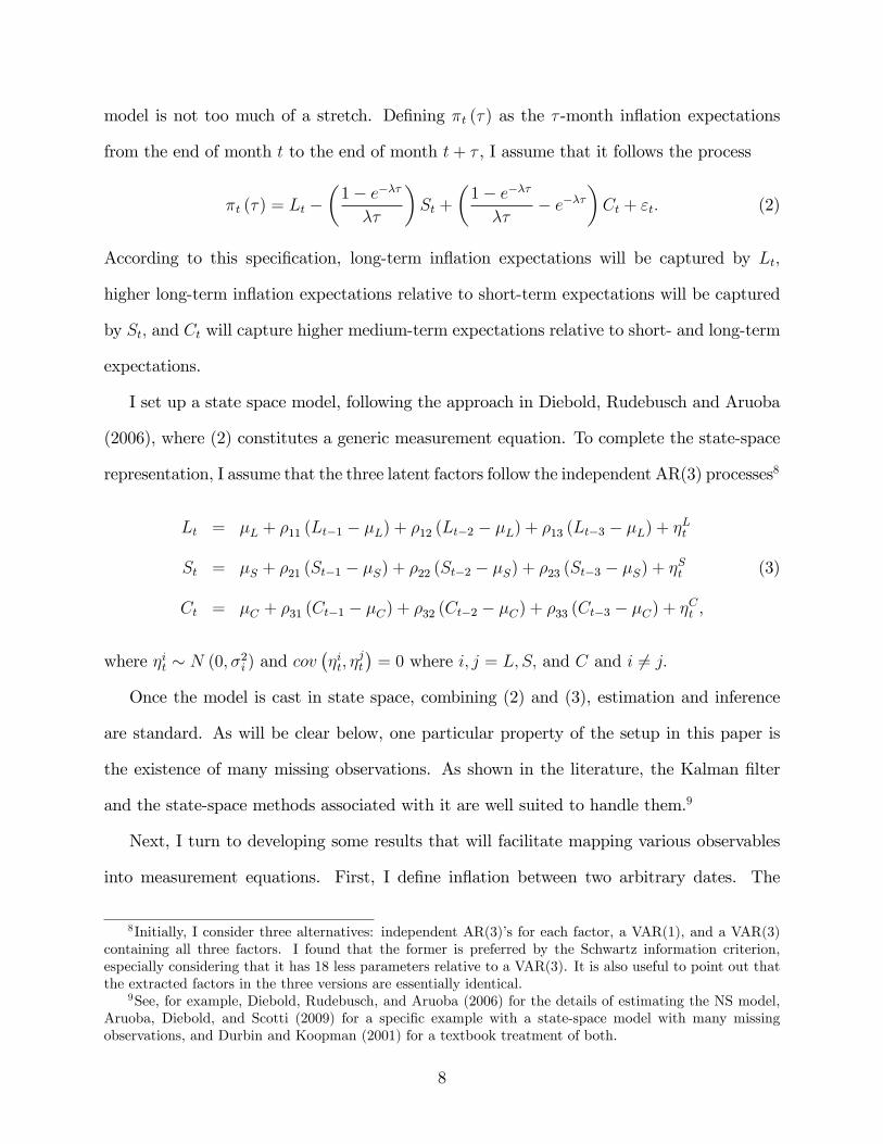
model is not too much of a stretch. De�ning �t (�) as the � -month in�ation expectations

from the end of month t to the end of month t+ � , I assume that it follows the process

�t (�) = Lt ��1� e�����

�St +

�1� e�����

� e����Ct + "t: (2)

According to this speci�cation, long-term in�ation expectations will be captured by Lt;

higher long-term in�ation expectations relative to short-term expectations will be captured

by St; and Ct will capture higher medium-term expectations relative to short- and long-term

expectations.

I set up a state space model, following the approach in Diebold, Rudebusch and Aruoba

(2006), where (2) constitutes a generic measurement equation. To complete the state-space

representation, I assume that the three latent factors follow the independent AR(3) processes8

Lt = �L + �11 (Lt�1 � �L) + �12 (Lt�2 � �L) + �13 (Lt�3 � �L) + �Lt

St = �S + �21 (St�1 � �S) + �22 (St�2 � �S) + �23 (St�3 � �S) + �St (3)

Ct = �C + �31 (Ct�1 � �C) + �32 (Ct�2 � �C) + �33 (Ct�3 � �C) + �Ct ;

where �it � N (0; �2i ) and cov��it; �

jt

�= 0 where i; j = L; S; and C and i 6= j:

Once the model is cast in state space, combining (2) and (3), estimation and inference

are standard. As will be clear below, one particular property of the setup in this paper is

the existence of many missing observations. As shown in the literature, the Kalman �lter

and the state-space methods associated with it are well suited to handle them.9

Next, I turn to developing some results that will facilitate mapping various observables

into measurement equations. First, I de�ne in�ation between two arbitrary dates. The

8Initially, I consider three alternatives: independent AR(3)�s for each factor, a VAR(1), and a VAR(3)containing all three factors. I found that the former is preferred by the Schwartz information criterion,especially considering that it has 18 less parameters relative to a VAR(3). It is also useful to point out thatthe extracted factors in the three versions are essentially identical.

9See, for example, Diebold, Rudebusch, and Aruoba (2006) for the details of estimating the NS model,Aruoba, Diebold, and Scotti (2009) for a speci�c example with a state-space model with many missingobservations, and Durbin and Koopman (2001) for a textbook treatment of both.

8

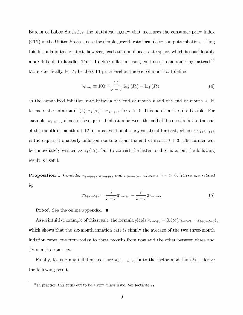
Bureau of Labor Statistics, the statistical agency that measures the consumer price index

(CPI) in the United States�uses the simple growth rate formula to compute in�ation. Using

this formula in this context, however, leads to a nonlinear state space, which is considerably

more di¢ cult to handle. Thus, I de�ne in�ation using continuous compounding instead.10

More speci�cally, let Pt be the CPI price level at the end of month t: I de�ne

�t!s � 100�12

s� t [log (Ps)� log (Pt)] (4)

as the annualized in�ation rate between the end of month t and the end of month s: In

terms of the notation in (2), �t (�) � �t!t+� for � > 0. This notation is quite �exible. For

example, �t!t+12 denotes the expected in�ation between the end of the month in t to the end

of the month in month t + 12; or a conventional one-year-ahead forecast, whereas �t+3!t+6

is the expected quarterly in�ation starting from the end of month t + 3: The former can

be immediately written as �t (12) ; but to convert the latter to this notation, the following

result is useful.

Proposition 1 Consider �t!t+s, �t!t+r; and �t+r!t+s where s > r > 0: These are related

by

�t+r!t+s =s

s� r�t!t+s �r

s� r�t!t+r: (5)

Proof. See the online appendix.

As an intuitive example of this result, the formula yields �t!t+6 = 0:5�(�t!t+3 + �t+3!t+6) ;

which shows that the six-month in�ation rate is simply the average of the two three-month

in�ation rates, one from today to three months from now and the other between three and

six months from now.

Finally, to map any in�ation measure �t+�1!t+�2 in to the factor model in (2), I derive

the following result.

10In practice, this turns out to be a very minor issue. See footnote 27.

9

Proposition 2 An in�ation measure �t+�1!t+�2 where � 2 > � 1 � 0 can be written as

�t+�1!t+�2 = Lt +e���1 � e���2� (� 2 � � 1)

(Ct � St) +�� 1e

���1 � � 2e���2� 2 � � 1

�Ct: (6)

Proof. See the online appendix.

As should be clear from inspecting (6), using continuous compounding, I preserve the

linearity of the state-space system, which would not be possible with a simple growth formula.

2.2 Measurement Equations

With the result of Proposition 2 in hand, all that remains to be done is to map observed

measures of in�ation expectations into the framework described so far. Letting xit be a

generic observable, this amounts to writing

xit =�f iL f iS f iC

�0@ LtStCt

1A+ "it;where ff iL; f iS; f iCg are the loadings on the three factors and "it � N (0; �2i ) is an idiosyncratic

error term, which accounts for deviations from the factor model. Survey-speci�c details are

provided in the online appendix.

2.3 State-Space System and Methodology

The preceding section and the details in the appendix showed the measurement equations of

the observable variables I use in my analysis �all in all, 37 variables. It is important to note

that the matrix of observables is considerably sparse due to the quarterly frequency of the

SPF and the fact that I used multiple observable variables for a given forecast. Combining

all the measurement equations and the transition equation for the three factors, I obtain a

state-space system

xt = Z�t + "t (7)

(�t � �) = T (�t�1 � �) + �t (8)

10

with

"t � N (0;H) and �t � N (0;Q) ; (9)

where the notation follows the standard notation in Durbin and Koopman (2001). The

vector xt is a 37 � 1 vector containing all observed variables in period t; and �t is a 9 � 1

vector that collects the three in�ation expectation factors and their two lags in period t :

�t =�Lt St Ct Lt�1 St�1 Ct�1 Lt�2 St�2 Ct�2

�0: (10)

The "t are the measurement errors, and thus H is a diagonal matrix with

H = diag��21; �

22; :::; �

237

�: (11)

The measurement matrix Z collects the factor loadings described in the online appendix and

is given by

Z =

26664f 1L f 1S f 1C 0 0 0 0 0 0f 2L f 2S f 2C 0 0 0 0 0 0...

......

..................

f 37L f 37S f 37C 0 0 0 0 0 0

37775 : (12)

The transition matrix T takes the form

T =

26666666666664

�11 0 0 �12 0 0 �13 0 00 �21 0 0 �22 0 0 �23 00 0 �31 0 0 �32 0 0 �331 0 0 0 0 0 0 0 00 1 0 0 0 0 0 0 00 0 1 0 0 0 0 0 00 0 0 1 0 0 0 0 00 0 0 0 1 0 0 0 00 0 0 0 0 1 0 0 0

37777777777775; (13)

and the constant � is given by

� =��L �S �C 0 0 0 0 0 0

�0: (14)

11

Finally, Q is a diagonal matrix with

Q = diag��Lt ; �

St ; �

Ct ; 0; 0; 0; 0; 0; 0

�: (15)

The model is estimated using maximum likelihood via the prediction-error decomposition

and the Kalman �lter. A total of 53 parameters are estimated, where all but 16 of these

parameters are measurement error variances. The smoothed estimates of the level, slope,

and curvature factors are obtained using the Kalman smoother.

2.4 Term Structure of Real Interest Rates

The Fisher equation links the nominal interest rate to the real interest rate and expected

in�ation. Generalizing to a generic maturity, I can write it as

yt (�) = rt (�) + �t (�) ; (16)

where yt (�) and rt (�) are the nominal and real continuously compounded interest rates or

yields for a bond that is purchased in period t and matures in period t+� : It is important to

note that by decomposing the nominal rate as above, I implicitly include the in�ation risk

premium in rt (�) : In Section 4.2 I discuss how this approach may a¤ect my �ndings.

Since I already obtained �t (�) above, all I need to do to obtain the term structure of

real interest rates is to obtain the term structure of nominal interest rates. To that end, I

could simply use (1) along with data on yields. Instead, I use the estimated yield curve as

computed by the Board of Governors of the Federal Reserve System, following Gürkaynak,

Sack, and Wright (2007). This yield curve is estimated using a generalized speci�cation of

the Nelson-Siegel model, the so-called Nelson-Siegel-Svensson speci�cation, which adds one

more factor to the original Nelson-Siegel model. More speci�cally, the measurement equation

12

becomes

yt (�) = Lyt ��1� e��1;t��1;t�

�Syt +

�1� e��1;t��1;t�

� e��1;t��Cy1;t (17)

+

�1� e��2;t��2;t�

� e��2;t��Cy2;t;

which simpli�es to (1) when �2;t = 0: Unlike the dynamic approach I take in this paper, or the

approaches in Diebold and Li (2005) or Diebold, Rudebusch, and Aruoba (2006), Gürkaynak,

Sack and Wright (2007) treat Lyt ; Syt ; C

y1;t; C

y2;t; �1;t; �2;t as parameters and estimate (17) every

period. These parameters are reported for every day since June 1961, which enables me to

compute yt (�) for any arbitrary maturity � : In turn, I compute the continuously compounded

real interest curve, rt (�) ; using (16).

3 In�ation Expectations Curve

The state-space model presented in the previous section is estimated on a sample that covers

the period from January 1992 through July 2013. The starting point of the sample is dictated

by the availability of the 10-year forecast from the SPF. All raw data are converted to

annualized percentage rates.11

3.1 Estimation Results

Table 1 presents the estimated parameter values. Panel (a) shows the estimated transition

equation parameters. The level factor is a near unit root (but covariance stationary), with the

smallest root of the characteristic polynomial slightly above unity. The slope and curvature

factors are also covariance stationary, and all three factors have both imaginary and real

roots. The long-run average of the level factor is just above 3%: The level factor captures

the very long-run in�ation expectations, and the estimated value re�ects the higher in�ation

expectations in the early 1990s due to the high levels of in�ation in the 1980s. The average

11When I carried out the estimation using a longer sample, the results for the post-1992 period werevirtually identical to the results presented here.

13

slope of the in�ation expectations curve, which is de�ned as the di¤erence between long-term

and short-term expectations, is mildly positive at 36 basis points. The curvature factor has

roughly a zero mean. The variances of the transition equation innovations are very small.

Panel (b) of Table 1 shows that � is estimated as 0:16; which means that the loading on the

curvature factor is maximized at just over 11 months. Two broad conclusions emerge from

looking at the measurement error variances. First, as the forecast horizon of the variable

increases, the measurement error variances become smaller, indicating a better �t of the

model. Second, the Michigan Survey variables display measurement error variances that

are about two orders of magnitude bigger than those for other sources at similar forecast

horizons. This means that there is a signi�cant mismatch between Michigan Survey variables

and other forecasts, which is apparent when one plots, for example, the one-year Michigan

Survey and the SPF forecasts.12

Given these estimated parameters, I obtain estimates of the three factors using the

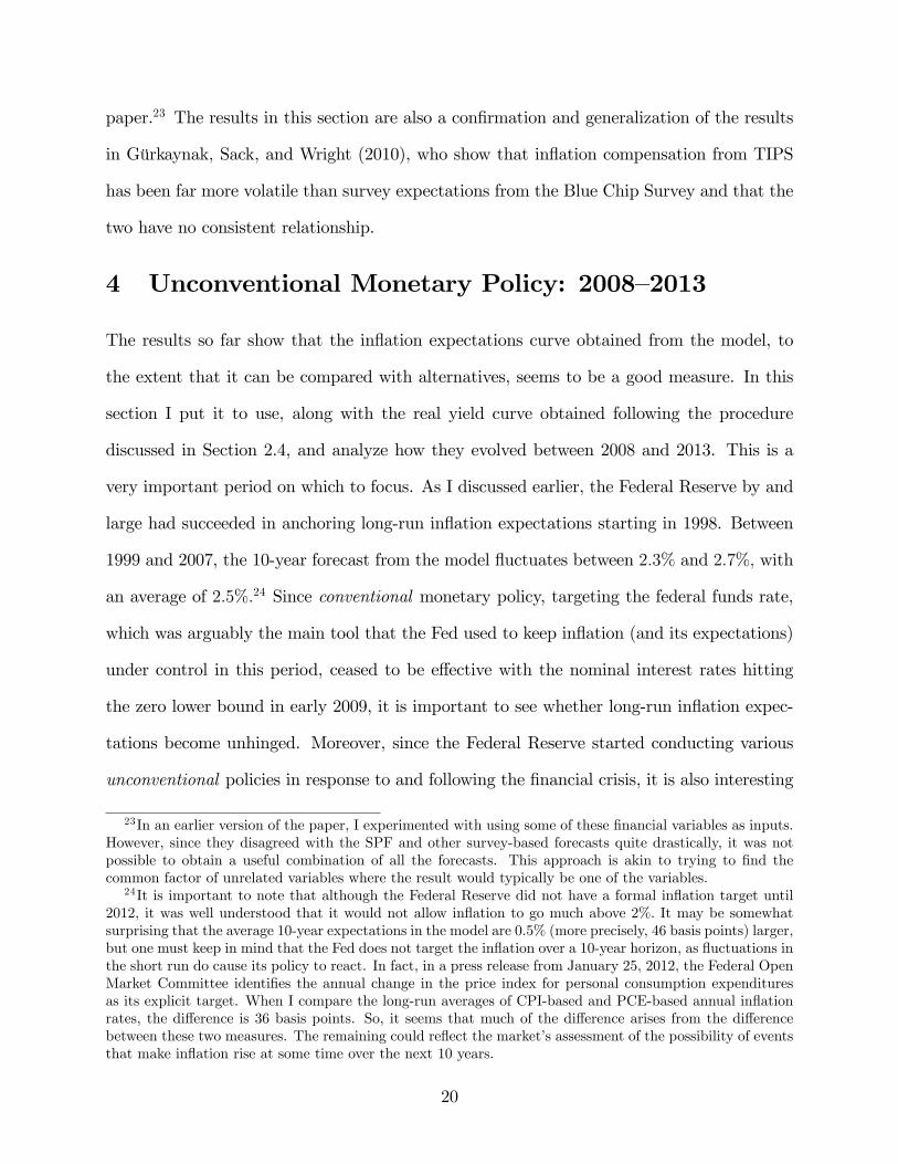
Kalman smoother, which are presented in Figure 1.13 As expected, the level factor (long-

run in�ation expectations) has a downward trend that �attens out by the early 2000s, after

which point it stays around 2.4%. The slope factor is positive for much of the sample, falling

below zero just before the 2001 recession, in 2006, and during the Great Recession, prior to

the �nancial crisis of 2008. As I show in detail in Section 4.1, during the �nancial crisis the

in�ation expectations curve sharply steepens, with much of the movement coming from the

short end. This is also visible in this �gure as the sharp increase in the slope near September

2008. The curvature factor has smaller �uctuations, and except for 2003 and the time fol-

lowing the �nancial crisis, where it was negative, it remains near zero for extended periods.

In fact, it seems that the curvature factor is negative in the early parts of recoveries after

12This is in line with the �ndings of Ang, Bekaert, and Wei (2007), who conclude that the professionalsuniformly beat the consumers in forecasting in�ation.

13In all �gures the two NBER recessions in the sample are shown with gray shading, and September 2008is shown with a vertical line. The latter is arguably the height of the �nancial crisis, and signi�cant changesoccur in both the in�ation forecasts and the �nancial variables introduced below. Also, where relevant, I usered dashed lines to denote pointwise 95% con�dence bands.

14

recessions, indicating that the in�ation expectations curve is U-shaped.

The main output from the estimation that is of interest is the in�ation expectations curve

itself. I focus on the post-2008 period in Section 4.1. In Figure 2, I show the time series of

some selected in�ation expectations: those at a 6-month and at 1-, 5-, and 10-year horizons.

In addition to the decline since the 1990s in all horizons, it is also apparent that as the

forecast horizon increases, the forecasts become smoother.

3.2 Comparison of Forecasts

In this section I compare the forecasts from the model with some alternatives. First, I

present results that compare the model�s forecasts with some of the survey inputs that enter

the model. This approach will demonstrate the bene�t of combining multiple forecasts,

which goes beyond the standard result where combining multiple forecasts improves forecast

accuracy. The inputs of the model provide information about various parts of the in�ation

expectations curve, with very few overlaps. In that sense, combining them will not be the

same as combining forecasts of the same object; rather it will be combining the information

in nearby forecast horizons. Second, I compare them with measures obtained from �nancial

variables. These variables are followed widely and considered by many as gauges of the

market�s in�ation expectations.

I present two sets of results. Figures 3, 4, and 5, each with two panels, show plots of the

forecasts from the model, the actual in�ation that was realized, and a number of alternative

measures. Table 2 presents formal forecast comparison test results using realized in�ation.

The latter is a useful exercise, since the ultimate goal of the technology developed in this

paper is to construct good forecasts of in�ation at various horizons.14 To remind the readers,

in what follows an N -month forecast refers to the in�ation expectations between the present

14One may take the point of view that if the underlying in�ation forecasts are not good in a forecastaccuracy sense, then the resulting combination would not be good either, and this is not necessarily aproblem. I want to demonstrate, however, that the resulting in�ation forecasts indeed have good forecastingproperties.

15

and N months from now. The �rst panel of Table 2 shows that the model forecast is superior

to a random walk (no-change) forecast and is statistically signi�cant for all but the 10-year

forecast.

3.2.1 Comparison with Inputs

The top panel of Figure 3 shows the one-year forecast and various alternative measures. As

inputs, it shows the implied Blue Chip forecast and a variable from the SPF.15 As expected,

the model forecast closely follows the inputs and is much less volatile than actual in�ation.16

The mean model forecast is identical to that of actual in�ation, a property it shares with

the Blue Chip forecast. The top panel of Figure 4 shows the 10-year model forecast and

the approximate forecast from the SPF, but since there is only ten common observations, it

is di¢ cult to reach any conclusions.17 The top panel of Figure 5 shows the ten-year model

forecast and the approximate forecast from the SPF. In the earlier part of the sample, roughly

until 1998, the SPF forecast and the model forecast are signi�cantly above actual in�ation.

As is well known, this result is due to the overhang from the high-in�ation period of the

1980s. After 1998 long-run in�ation expectations start to get anchored near the Federal

Reserve�s implicit target of 2%:18 The model forecast closely follows the approximate SPF

forecast, but it also uses the long-term Blue Chip forecasts (not shown) that have information

about nearby horizons.

15The implied Blue Chip forecast is simply the average of the t! t+ 3; t+ 3! t+ 6; t+ 6! t+ 9; andt+9! t+12 forecasts and is available quarterly. For the SPF I use the Annual �B�forecast for the fourthquarter of every year which corresponds to t+ 1! t+ 13 forecast and is available annually.

16The actual in�ation measure is the appropriate di¤erence of the natural logarithm of CPI, as extractedfrom FRED in December 2013, with the FRED code CPIAUCSL.

17The forecast from the SPF is approximate since it combines three of the 5-year forecasts which are fromperiod t to t+52; t+55; and t+58: A similar comment applies to the approximate 10-year forecast in Figure5.

18The Federal Reserve emphasizes the in�ation rate based on personal consumption expenditures (PCE)and since January 2012 it has an explicit target of 2% based on this measure. Although PCE in�ation uses thesame underlying source data, it uses weights di¤erent from the CPI in�ation. Their levels are also somewhatdi¤erent, with CPI in�ation being slightly larger than PCE in�ation on average. The analysis in this paperis done using CPI in�ation, since historical forecasts for PCE are not available at multiple frequencies. Seealso footnote 23.

16

The �rst panel of Table 2 shows the forecast comparison results versus some of the

inputs. The �rst column reports the root-mean-squared error (RMSE) of the model forecast,

the second column reports the RMSE of the alternative measure considered and the third

column shows the number of observations available for each comparison. Boldface in a given

column indicate the rejection of the null of equal forecast accuracy in favor of the forecast in

that column using the Diebold and Mariano (1995) test with the squared-error loss function.

The results show that the model forecast is a better forecast in terms of RMSE relative to

the three inputs considered, though this is not statistically signi�cant at the 5% signi�cance

level.

3.2.2 Comparison with Measures Derived from Financial Variables

It is well understood that many �nancial variables contain information about the market

participants� in�ation expectations. Perhaps the two �nancial instruments that have the

most information are in�ation swaps and Treasury In�ation-Protected Securities (TIPS).

An in�ation swap is an agreement in which one party makes periodic payments to another

party, which are linked to in�ation realized in the future, in exchange for a �xed payment up

front. In a perfect world, one without risk premia, and one in which all assets are arbitrarily

liquid, this �xed payment will be a good estimate of the two participants�in�ation forecasts.

TIPS, on the other hand, are bonds issued by the U.S. Treasury, with yields that are linked

to future realized in�ation rates. Again, in a perfect world, the di¤erence between the yield

on a TIPS at a certain maturity and the U.S. Treasury nominal yield at the same maturity,

the so-called break-even rate (or in�ation compensation), will be a good estimate for the

in�ation expectations of the market.19

As it turns out, we do not live in such a perfect world �one without risk premia and

arbitrarily liquid asset markets. The liquidity of the TIPS market has changed signi�cantly

19The TIPS rate is linked explicitly to seasonally adjusted CPI. Swap rates are linked to seasonallyunadjusted CPI. Although there does not seem to be any discernible seasonality in swap rates, this certainlycomplicates models in which swap rates are used.

17

since its inception, which makes it very di¢ cult to use the break-even rate as a direct

estimate of in�ation expectations. Similar problems also plague the in�ation swaps market.20

D�Amico, Kim, and Wei (2010) utilize a no-arbitrage asset pricing model to produce market

in�ation expectations using the TIPS break-even rate, as well as nominal U.S. Treasury

yields. This measure is widely used as a clean version of the TIPS break-even rate. Haubrich,

Pennacchi, and Ritchken (2012) follow an approach that is broadly similar, in that they

consider an asset pricing model that has implications for nominal yields and swap rates, and

the model is estimated using these observables, as well as some forecasts from the Blue Chip

Economic Indicators and the SPF.21

The bottom panel of Figure 3 shows the one-year swap rate and the results from Haubrich,

Pennacchi, and Ritchken (2012), labeled as �Cleveland Fed.�Two things are very clear. The

Cleveland Fed forecast and the swap rate, when it is available, are signi�cantly more volatile

than the model forecast. Also, the swap rate takes a signi�cant dive near the �nancial crisis,

falling to nearly �4%; while the SPF and model forecasts remain slightly above 1%: It is

quite clear that the raw swap rate su¤ers from the problems I list above. Although not as

extreme as the swap rate, the Cleveland Fed forecast also displays similar behavior, falling

below zero in early 2009.

Figure 4 shows the �ve-year swap rate, TIPS break-even rate, and the results from

D�Amico, Kim, and Wei (2010), labeled �DKW In�ation Expectation.�Also shown is the

Cleveland Fed forecast, with TIPS-related variables in the top panel and the swap-rate-

related variables in the bottom panel. The TIPS break-even rate clearly displays very di¤er-

20David Lucca and Ernst Schaumburg provide a good summary of these problems and some others thatmake TIPS and swap rates noisy indicators of in�ation expectations. See David Lucca and Ernst Schaumburg,�What to Make of Market Measures of In�ation Expectations?�Liberty Street Economics (blog), FederalReserve Bank of New York, August 15, 2011, http://libertystreeteconomics.newyorkfed.org/2011/08/what-to-make-of-market-measures-of-in�ation-expectations.html.

21Both D�Amico, Kim, and Wei (2010) and Haubrich, Pennacchi, and Ritchken (2012) start their esti-mation prior to the introduction of TIPS and swaps, respectively, using nominal yields as the only �nancialasset. As such, their reported in�ation expectations can be considered as cleaned TIPS and swaps only after1999 for TIPS and 2004 for swaps.

18

ent behavior before 2003 and again after the �nancial crisis in 2008 relative to both actual

in�ation and the model forecast. A similar conclusion also applies for the swap rate, which

is available for a shorter sample. Both rates fall below zero during the �nancial crisis. Both

DKW and the Cleveland Fed forecasts behave much better relative to the raw �nancial vari-

ables, although especially after 1998, when the long-run in�ation expectations start to settle,

they are more volatile relative to the model forecast. Figure 5 shows the same variables for

the 10-year horizon, and by and large the same conclusions apply.

The rest of Table 2 shows forecast comparison results for the variables discussed in

this section. The raw �nancial variables, shown in the third and fourth panels, produce

substantially worse forecasts relative to the model forecast, with improvements in the RMSEs

of the latter as large as 67% for the 10-year TIPS break-even rate. Looking deeper to

the source of the large RMSE for this particular variable, it is twice as volatile as the

model forecast and that the bias is �0:3% versus 0:1% for the model forecast. The DKW

and Cleveland Fed forecasts produce results that are much better, with RMSEs that are

roughly half of the raw �nancial variables and near the values attained by the model forecast.

The model forecast comes out signi�cantly more accurate than the two-year Cleveland Fed

forecast, with the model forecast producing better RMSEs in all other cases. The model

forecast is signi�cantly more accurate than the 5-year and 10-year DKW forecast, whereas

for the 2-year forecast the DKW forecast produces a lower RMSE, although the di¤erence

in forecast accuracy is not statistically signi�cant.22

I view the results of this section as making a strong case for the usefulness of the model

forecast relative to a number of alternatives related to the �nancial markets. This strong

case is also why I chose not to use any �nancial variables in the model developed in this

22For the DKW forecast, I restrict the results to the sample starting in 1999, when actual TIPS dataare available. If I start the forecast comparison in 1992, the DKW forecast produces a lower RMSE withan insigni�cant di¤erence in forecast accuracy. In the very early part of the sample, the model forecastsigni�cantly overshoots the longer-term forecasts due to the overhang I mentioned above. When I redo thecomparison starting in 1994 instead of 1992, the model forecast has lower RMSE than the DKW forecast forall three horizons considered.

19

paper.23 The results in this section are also a con�rmation and generalization of the results

in Gürkaynak, Sack, and Wright (2010), who show that in�ation compensation from TIPS

has been far more volatile than survey expectations from the Blue Chip Survey and that the

two have no consistent relationship.

4 Unconventional Monetary Policy: 2008�2013

The results so far show that the in�ation expectations curve obtained from the model, to

the extent that it can be compared with alternatives, seems to be a good measure. In this

section I put it to use, along with the real yield curve obtained following the procedure

discussed in Section 2.4, and analyze how they evolved between 2008 and 2013. This is a

very important period on which to focus. As I discussed earlier, the Federal Reserve by and

large had succeeded in anchoring long-run in�ation expectations starting in 1998. Between

1999 and 2007, the 10-year forecast from the model �uctuates between 2:3% and 2:7%; with

an average of 2:5%:24 Since conventional monetary policy, targeting the federal funds rate,

which was arguably the main tool that the Fed used to keep in�ation (and its expectations)

under control in this period, ceased to be e¤ective with the nominal interest rates hitting

the zero lower bound in early 2009, it is important to see whether long-run in�ation expec-

tations become unhinged. Moreover, since the Federal Reserve started conducting various

unconventional policies in response to and following the �nancial crisis, it is also interesting

23In an earlier version of the paper, I experimented with using some of these �nancial variables as inputs.However, since they disagreed with the SPF and other survey-based forecasts quite drastically, it was notpossible to obtain a useful combination of all the forecasts. This approach is akin to trying to �nd thecommon factor of unrelated variables where the result would typically be one of the variables.

24It is important to note that although the Federal Reserve did not have a formal in�ation target until2012, it was well understood that it would not allow in�ation to go much above 2%: It may be somewhatsurprising that the average 10-year expectations in the model are 0.5% (more precisely, 46 basis points) larger,but one must keep in mind that the Fed does not target the in�ation over a 10-year horizon, as �uctuations inthe short run do cause its policy to react. In fact, in a press release from January 25, 2012, the Federal OpenMarket Committee identi�es the annual change in the price index for personal consumption expendituresas its explicit target. When I compare the long-run averages of CPI-based and PCE-based annual in�ationrates, the di¤erence is 36 basis points. So, it seems that much of the di¤erence arises from the di¤erencebetween these two measures. The remaining could re�ect the market�s assessment of the possibility of eventsthat make in�ation rise at some time over the next 10 years.

20

to analyze the impact of these policies on the in�ation expectations curve.25 Finally, some, if

not most of these unconventional policies were aimed at providing additional stimulus for the

real side of the economy, and by looking at the real yield curve, we can investigate whether

these policies they succeeded.26

I focus on �ve speci�c events in this period: the �nancial crisis, the initial quantitative

easing (QE1), QE2, Operation Twist, and the Federal Reserve�s explicit adoption of an

in�ation target.27 Although determining the start of the �nancial crisis is di¢ cult, I use

September 2008, which is when much of the major events happened. QE1, which consists of

a number of large-scale asset purchase programs, started in December 2008 and concluded

by August 2010, after having increased the balance sheet of the Fed by some $1.75 trillion.

QE2, which consisted of a plan to purchase $600 billion of long-term Treasury securities,

was put in place between November 2010 and June 2011. Operation Twist (formally known

as the Maturity Extension Program) aimed at increasing the maturity of the Fed�s assets

and was in e¤ect between September 2011 and December 2012. Finally, the Federal Reserve

announced a formal in�ation target of 2% on January 25, 2012. Below, I look at how the

in�ation expectations and real interest rate curves change around these dates. One small

caveat to note: it is conceivable that some other events, in addition to and unrelated to

the Fed programs, may have an impact on in�ation expectations and real interest rates.

However, it is di¢ cult to argue that events other than actions by the Federal Reserve may

have as large an impact on in�ation expectations, especially during the period I consider. A

25Some (perhaps all) of this analysis can be conducted by looking at the survey forecasts I use in my modeland at some �nancial variables. However, the previous section showed that based on historical forecastingperformance, both sets of measures are expected to be inferior to the model forecast. Also, the surveyvariables for the long-horizon forecasts are only available quarterly, which severely restricts their use for thispurpose.

26Here I have in mind a very general model where the real interest rate is one of the key determinantsof current economic activity. A decline in the real interest rate stimulates private consumption demand bymaking consumption cheaper today as opposed to the future, and it also boosts investment by reducing theopportunity cost of funds used for investment.

27In�ation expectations and real interest rates at various key horizons are shown in Tables 3 and 4 in theonline appendix for every month starting in January 2008.

21

similar albeit less strong case can be made for the real interest rate.

4.1 In�ation Expectations Curve

Figure 6 plots in�ation expectations obtained from the model for some key horizons, and

Figure 8 in the online appendix shows the same information, but with the whole in�ation

expectations curve plotted for various key dates. In Figure 6 the �nancial crisis is shown with

a vertical line in September 2008, the three Fed programs are shown with yellow shading and

the announcement of the formal in�ation target is denoted with a dashed-dotted vertical line.

The �nancial crisis causes drastic changes in in�ation expectations in the short and medium

horizons but not as much in the long horizons. In March 2008 the in�ation expectations

curve is �at at around 2:4%: In the summer, the short end (e.g., the six-month horizon)

edges up to almost 3%; re�ecting the concern about rising energy prices. After the onset of

the crisis and the decline of energy prices in September, the short end of the curve takes a

big plunge, falling to just above 1% in December. Throughout the crisis, the long end of the

curve remains relatively stable, especially compared with the short end: the 10-year forecast

decreases from 2:5% in July 2008 to 2:4% in December 2008.

When viewed in a low frequency, the 10-year forecast does not seem to be a¤ected signif-

icantly by the �nancial crisis: in the period September 2008-July 2013, it �uctuates between

2:2% and 2:4%;with an average of 2:3%, a decline of only 14 basis points. Using the model, I

am able to compute the 3-year-to-10-year (starting in year 3, ending in year 10) and 6-year-

to-10-year forecasts, which are shown as dashed lines in this �gure. These forecasts remain in

the pre-crisis levels of around 2:4%: Thus, much of the (already small) decline in the 10-year

expectations arises from the expected decline during the �rst 2 to 5 years. It is also worth

mentioning that as the size of the Fed�s balance sheet grew rapidly and continuously for

much of this period, which could possibly lead to higher in�ation, the long-run expectations

show no upward trend. My results are in line with Merten�s (2011) results, which show that

22

trend in�ation does not change by much during the crisis.

Turning to the e¤ects of QE1 and QE2, they have similar and large e¤ects on the slope

of the in�ation expectations curve, and small but opposite e¤ects on the level of the in�ation

expectations curve. In particular, QE1 increases the six-month expectations from around 1%

in December 2008 to over 1:5% in August 2010 while mildly reducing longer horizons. QE2,

on the other hand, increases the six-month expectations from around 1:5% in November 2010

to around 2:1% in June 2011; with milder increases in all other horizons. Figure 8 shows

that the e¤ect of QE1 on the curve is a �attening with a slight shift downward in the long

end, while QE2 also �attens the curve but shifts it upward. None of these changes, however,

bring the in�ation expectations curve close to its pre-crisis shape, despite the strong level of

mean reversion that is built into the model. One way to see this e¤ect is by computing a

counterfactual where the model evolves without shocks starting in December 2008 and then

comparing it with the actual evolution. This approach reveals that in�ation expectations of

all horizons are consistently below the counterfactual, even though they increase relative to

the onset of the crisis.

Operation Twist, whose goal was to increase the maturity structure of the Fed balance

sheet via purchases of long-term securities and the sale of short-term securities, did not a¤ect

in�ation expectations in any signi�cant way. Figure 8 shows that the announcement of the

formal in�ation target in January 2012 seems to shift the level of the in�ation expectations

curve upward by about 10 basis points and reduce the slope by about 50 basis points. Figure

6 shows, however, that the �attening of the curve is part of a longer-term trend that covers

the �rst half of 2012. We can thus conclude that the announcement of the formal in�ation

target does not lead to much change in in�ation expectations.

23

4.2 Real Interest Rate Curve

Paralleling the analysis in the previous section, Figure 7 plots some key real interest rates

over the period 2008-2013, and Figure 9 in the online appendix shows the full real interest

rate curve at various key points in time.

Before turning to the results, I want to explain how I handle the issue I pointed out in

Section 2.4. The real interest rate that I compute via (16) in principle inherits the in�ation

risk premium from nominal yields. Identifying and removing the risk premium requires a

�nancial model. Fortunately, as I explained above, the goal of D�Amico, Kim, and Wei

(2010) is precisely to identify the risk premium and liquidity premium components of the

TIPS in�ation compensation to arrive at in�ation expectations. These components are

available for the 2-year, 5-year, and 10-year measures. In Figure 7 the dashed lines for these

horizons show the real interest rate with the in�ation risk premium removed. Although this

concern is valid ex ante, the �gure shows that for the conclusions I reach below, the risk

premium is small enough not to matter.

In January 2008, as the U.S. economy was already slowing down but before the peak of

the �nancial crisis, all real interest rates were positive with a U-shaped real interest curve.

As the Fed was reducing the short end of the nominal yield curve throughout 2008, the whole

real yield curve also shifts downward signi�cantly. As of December 2008, the real interest rate

for horizons up to seven years is negative, with the two-year rate around �1:4%: Thus, the

combination of the �nancial crisis and the Fed�s conventional response leads to a downward

shift of the real yield curve, with the short end of the curve remaining higher than the middle.

QE1 reduces the short end of the curve, bringing the six-month rate to around �1:3%

by the end of the program, at its peak leading to a decline of almost a full percentage point.

Despite �uctuations throughout the program, real interest rates of longer maturities remain

largely the same after the program ends, although at lower levels relative to those before the

�nancial crisis. QE2 further reduces the short end of the curve by another 0:6%; with the

24

longer maturities behaving the same way as they did during QE1. Since the end of QE2, the

six-month real interest rates hover just above �2%: Considering that the average six-month

real interest rate in the period 1992-2007 is 1:5% with a minimum of �0:8% obtained in

December 2003, this very low level seems to be highly stimulative.

With Operation Twist, the Fed seems to bring the long end of the real interest rate curve

from around 0% to around �0:6%: Once again, the average and minimum of this rate in

the period 1992-2007 are 2:8% and 1:2%; respectively, and the long real rates are also highly

stimulative. Since the end of 2012, medium- and long-term real rates have been rising but

are still signi�cantly below their pre-crisis levels.

4.3 Summary

Here is a summary of the �ndings in this section:

� The �nancial crisis and the Fed�s conventional response reduced both in�ation ex-

pectations and real interest rates signi�cantly, with the distinct exception of in�ation

expectations of long horizons where the decline was very mild. Real interest rates

hit unprecedented negative levels for short and medium maturities, indicating that

the decline in nominal rates was transmitted to real rates by a less than one-to-one

response of in�ation expectations.

� Long-run in�ation expectations decline by 14 basis points in the 2008-2013 period

relative to the pre-crisis average. This small decline can be almost fully attributed to

changes in the short-term expectations as the 3-year-to-10-year and 6-year-to-10 year

expectations remain constant.

� As a reaction to QE1, and to some extent mean reversion, in�ation expectations of

short maturities rise by about 0:5% and by another 0:5% following QE2. Short-term

real rates continue to fall, reaching a low of �2% by the end of 2012. This rate is about

3:5% below the pre-crisis average.

25

� In reaction to QE1, longer-horizon in�ation expectations fall by about 0:1%; and in re-

action to QE2, they rise by about 0:2%: Despite some �uctuations during the programs,

the long-term real rates do not change as a result of these programs.

� Operation Twist does not lead to a change in in�ation expectations and reduces the

long-term real interest rates by about 0:6%; reaching �0:8% in the summer of 2012.

This rate is about 3:6% below the pre-crisis average.

� The announcement of the formal in�ation target does not a¤ect in�ation expectations

or real interest rates in any signi�cant way.

5 Conclusions

Starting in 2008, the Federal Reserve enacted unprecedented policies in response to the

biggest decline in economic activity since the Great Depression. The impact of these policies

on medium- to long-term in�ation are yet to be seen. In this paper I provide a statistically

e¢ cient and accurate way of aggregating survey-based in�ation expectations into an in�ation

expectations curve. I also compute a term structure of real interest rates, combining the

in�ation expectations curve with a nominal yield curve.

The resulting term structure of in�ation expectations proves capable of providing superior

forecasts relative to some of the popular alternatives that use �nancial variables, as well as

relative to some of the inputs used in the estimation. Thus, moving forward, this approach

seems to be a useful tool to gauge in�ation expectations at any arbitrary horizon.

I �nd that neither the �nancial crisis of 2008 nor the Federal Reserve policies that were

put in place during and after it a¤ected the long-run in�ation expectations, despite large

changes in shorter horizons. The Federal Reserve�s unconventional policies, especially QE1

and QE2, had a large e¤ect on the slope of the in�ation expectations curve, increasing

short-term expectations. As a result, these same policies reduced short-term real rates to

26

unprecedented levels. Operation Twist, on the other hand, reduced long-term real rates. All

in all, real interest rates of all horizons are about 3:5% lower than their pre-crisis averages,

indicating a massive stimulus to the economy.

From here, a number of further directions are possible. First, a reasonable approach may

be to consider non-Gaussian errors or stochastic volatility (or both) in the model. Second,

although the model in this paper explicitly excludes �nancial variables, there may be ways

of introducing them without worsening performance. For example, similar to but distinctly

di¤erent from what Christensen, Lopez, and Rudebusch (2012) do, one could model in�ation

expectations as I do here and add nominal yields that follow a Nelson-Siegel structure with

di¤erent factors. Finally, one could introduce information from various online prediction

markets. I leave these directions for future work.

References

[1] Ajello, A., L. Benzoni, and O. Chyruk (2012), �Core and �Crust�: Consumer Prices and

the Term Structure of Interest Rates,�mimeo, Federal Reserve Bank of Chicago.

[2] Ang, A., G. Bekaert, and M. Wei (2007), �Do Macro Variables, Asset Markets, or

Surveys Forecast In�ation Better?�Journal of Monetary Economics, 54(4), 1163-1212.

[3] Aruoba, S.B., F.X. Diebold and C. Scotti (2009), �Real-Time Measurement of Business

Conditions,�Journal of Business and Economic Statistics, 27(4), 417-427.

[4] Chernov, M., and P. Mueller (2012), �The Term Structure of In�ation Expectations,�

Journal of Financial Economics, 106(2), 367-394.

[5] Christensen, J.H.E., J.A. Lopez, and G.D. Rudebusch (2010), �In�ation Expectations

and Risk Premiums in an Arbitrage-Free Model of Nominal and Real Bond Yields,�

Journal of Money, Credit and Banking, 42(s1), 143-178.

27

[6] Christensen, J.H.E., J.A. Lopez, and G.D. Rudebusch (2012), �Extracting De�ation

Probability Forecasts from Treasury Yields,�International Journal of Central Banking,

8(4), 21-60.

[7] D�Amico, S., D.H. Kim, and M. Wei (2010), �Tips from TIPS: The Informational Con-

tent of Treasury In�ation-Protected Security Prices,�Board of Governors of the Federal

Reserve System Finance and Economics Discussion Series, 2010-19.

[8] Diebold, F.X., and C. Li, (2006), �Forecasting the Term Structure of Government Bond

Yields,�Journal of Econometrics, 130(2), 337-364.

[9] Diebold, F.X., and R.S. Mariano (1995), �Comparing Predictive Accuracy,�Journal of

Business and Economic Statistics, 13(3), 253-263.

[10] Diebold F.X., and G.D. Rudebusch (2013), Yield Curve Modeling and Forecasting: The

Dynamic Nelson-Siegel Approach, Princeton University Press.

[11] Diebold, F.X., G.D. Rudebusch, and S.B. Aruoba (2006), �The Macroeconomy and the

Yield Curve: A Dynamic Latent Factor Approach,�Journal of Econometrics, 131(1-2),

309-338.

[12] Durbin, J., and S.J. Koopman (2001), Time Series Analysis by State Space Methods,

Oxford University Press.

[13] Faust, J., and J.H. Wright (2013), �Forecasting In�ation,� in Handbook of Economic

Forecasting, vol. 2 pt. A, ed. G. Elliott and A. Timmermann, 2-56, Elsevier.

[14] Gürkaynak, R.S., B. Sack, and J.H. Wright (2007), �The U.S. Treasury Yield Curve:

1961 to the Present,�Journal of Monetary Economics, 54(8), 2291-2304.

[15] Gürkaynak, R.S., B. Sack, and J.H. Wright (2010), �The TIPS Yield Curve and In�ation

Compensation,�American Economic Journal: Macroeconomics, 2(1), 70-92.

28

[16] Haubrich, J.G., G. Pennacchi, and P. Ritchken (2012), �In�ation Expectations, Real

Rates, and Risk Premia: Evidence from In�ation Swaps,�Review of Financial Studies,

25(5), 1588-1629.

[17] Mertens, E. (2011), �Measuring the Level and Uncertainty of Trend In�ation,�Board

of Governors of the Federal Reserve System Finance and Economics Discussion Series,

2011-42.

[18] Nelson, C.R., and A.F. Siegel (1987), �Parsimonious Modeling of Yield Curves,�Journal

of Business, 60(4), 473-489.

[19] Stark, T. (2010), �Realistic Evaluation of Real-Time Forecasts in the Survey of Profes-

sional Forecasters,�Federal Reserve Bank of Philadelphia Research Rap Special Report.

29

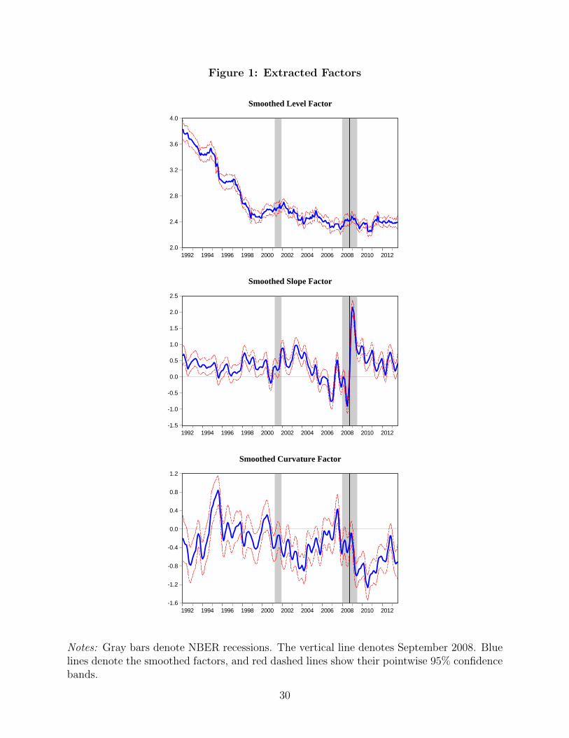
Figure 1: Extracted Factors

2.0

2.4

2.8

3.2

3.6

4.0

1992 1994 1996 1998 2000 2002 2004 2006 2008 2010 2012

Smoothed Level Factor

-1.5

-1.0

-0.5

0.0

0.5

1.0

1.5

2.0

2.5

1992 1994 1996 1998 2000 2002 2004 2006 2008 2010 2012

Smoothed Slope Factor

-1.6

-1.2

-0.8

-0.4

0.0

0.4

0.8

1.2

1992 1994 1996 1998 2000 2002 2004 2006 2008 2010 2012

Smoothed Curvature Factor

Notes: Gray bars denote NBER recessions. The vertical line denotes September 2008. Bluelines denote the smoothed factors, and red dashed lines show their pointwise 95% confidencebands.

30

Figure 2: Selected Inflation Expectations

1.0

1.5

2.0

2.5

3.0

3.5

4.0

92 94 96 98 00 02 04 06 08 10 12

6-Month Forecast

1.0

1.5

2.0

2.5

3.0

3.5

4.0

92 94 96 98 00 02 04 06 08 10 12

1-Year Forecast

1.0

1.5

2.0

2.5

3.0

3.5

4.0

92 94 96 98 00 02 04 06 08 10 12

5-Year Forecast

1.0

1.5

2.0

2.5

3.0

3.5

4.0

92 94 96 98 00 02 04 06 08 10 12

10-Year Forecast

Notes: Gray bars denote NBER recessions. The vertical line denotes September 2008. Bluelines denote the forecasts, and red dashed lines show their pointwise 95% confidence bands.

31

Figure 3: Comparison of One-Year Inflation Expectations with Inputs,Financial Variables, and Actual

-2

-1

0

1

2

3

4

5

92 94 96 98 00 02 04 06 08 10 12

Model Forecast Blue Chip Implied 0-->12SPF 1-->13 Actual

(a) Model, Inputs, and Actual

-2

-1

0

1

2

3

4

5

92 94 96 98 00 02 04 06 08 10 12

Model Forecast Cleveland FedSwap Actual

(b) Model, Financial Variables, and Actual

Notes: Gray bars denote NBER recessions. The vertical line denotes September 2008. Theswap rate (orange line) falls to -3.83% in December 2008, but the graph is truncated at -2%.

32

Figure 4: Comparison of Five-Year Inflation Expectations with Inputs,Financial Variables, and Actual

1.0

1.5

2.0

2.5

3.0

3.5

4.0

92 94 96 98 00 02 04 06 08 10 12

Model Forecast SPF Approximate 0-->60DKW Inflation Expectation TIPS Break-Even InflationActual

(a) Model Forecast, Input, Financial Variables, and Actual

1.0

1.5

2.0

2.5

3.0

3.5

4.0

92 94 96 98 00 02 04 06 08 10 12

Model Forecast Cleveland FedSwap Actual

(b) Model Forecast, Financial Variables, and Actual

Notes: Gray bars denote NBER recessions. The vertical line denotes September 2008. TheTIPS break-even rate (purple line) falls to −1.33%, and the swap rate (orange line) falls to−0.19% in December 2008, but the graph is truncated at 1%.

33

Figure 5: Comparison of 10-Year Inflation Expectations with Inputs, FinancialVariables, and Actual

1.0

1.5

2.0

2.5

3.0

3.5

4.0

92 94 96 98 00 02 04 06 08 10 12

Model Forecast SPF Approximate 0-->120DKW Inflation Expectation TIPS Break-Even InflationActual

(a) Model Forecast, Input, Financial Variables, and Actual

1.0

1.5

2.0

2.5

3.0

3.5

4.0

92 94 96 98 00 02 04 06 08 10 12

Model Forecast Cleveland FedSwap Actual

(b) Model Forecast, Financial Variables, and Actual

Notes: Gray bars denote NBER recessions. The vertical line denotes September 2008. TheTIPS break-even rate (purple line) falls to 0.52%, and the swap rate (orange line) falls to1.49% in December 2008, but the graph is truncated at 2%.

34

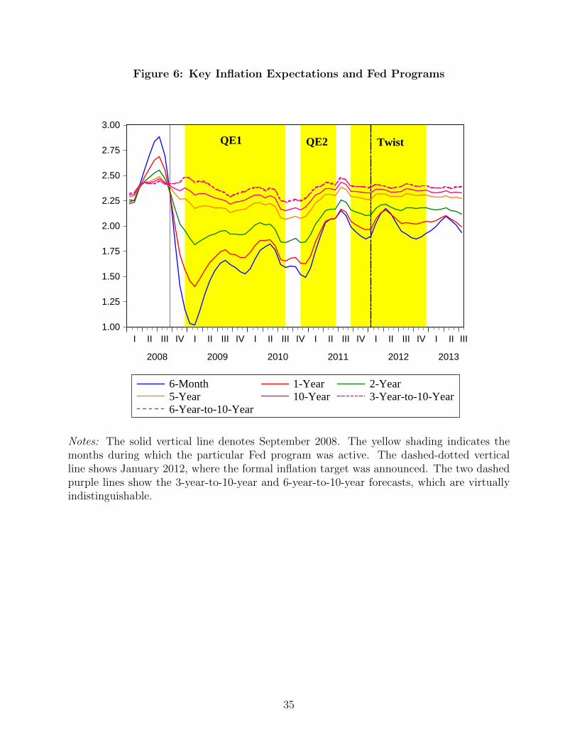
Figure 6: Key Inflation Expectations and Fed Programs

1.00

1.25

1.50

1.75

2.00

2.25

2.50

2.75

3.00

I II III IV I II III IV I II III IV I II III IV I II III IV I II III

2008 2009 2010 2011 2012 2013

6-Month 1-Year 2-Year5-Year 10-Year 3-Year-to-10-Year6-Year-to-10-Year

QE1 QE2 Twist

Key Inflation Expectations and Fed Programs

Notes: The solid vertical line denotes September 2008. The yellow shading indicates themonths during which the particular Fed program was active. The dashed-dotted verticalline shows January 2012, where the formal inflation target was announced. The two dashedpurple lines show the 3-year-to-10-year and 6-year-to-10-year forecasts, which are virtuallyindistinguishable.

35

Figure 7: Key Real Interest Rates and Fed Programs

-2

-1

0

1

2

I II III IV I II III IV I II III IV I II III IV I II III IV I II III

2008 2009 2010 2011 2012 2013

6-Month 1-Year 2-Year5-Year 10-Year

QE1 QE2 Twist

Key Real Interest Rates and Fed Programs

Notes: The solid vertical line denotes September 2008. The yellow shading indicates themonths during which the particular Fed program was active. The dashed-dotted verticalline shows January 2012, where the formal inflation target was announced. Dashed linesshow the real interest rate for the same horizon as the solid line, cleaned from the inflationrisk premium using the measure computed by D’Amico, Kim, and Wei (2010).

36

Table 1: Estimation Results

(a) Transition Equation

Level Slope Curvature

ρ11 1.00 ρ21 2.24 ρ31 2.13ρ12 -0.09 ρ22 -1.88 ρ32 -1.71ρ13 0.09 ρ23 0.60 ρ33 0.55

Roots of the Characteristic Polynomials

0.01 ± 3.34i, 1.00 0.99 ± 0.67i, 1.18 1.01 ± 0.81i, 1.09

µ1 3.02 µ2 0.36 µ3 -0.33

σ2L 0.002 σ2

S 0.004 σ2C 0.004

(b) Measurement Equation

λ = 0.16

SPF Quarterly Blue Chip Short-Run Blue Chip Long-Run

σ21 0.014 σ2

16 0.061 σ228 0.009

σ22 0.009 σ2

17 0.008 σ229 0.008

σ23 0.006 σ2

18 0.008 σ230 0.005

SPF Annual σ219 0.004 σ2

31 0.003σ24 0.009 σ2

20 0.016 σ232 0.001

σ25 0.009 σ2

21 0.010 σ233 0.002

σ26 0.005 σ2

22 0.008 σ234 0.003

σ27 0.016 σ2

23 0.003 σ235 0.002

SPF Five-Year σ224 0.006

σ28 0.043 σ2

25 0.013 Michiganσ29 0.031 σ2

26 0.006 σ236 0.787

σ210 0.016 σ2

27 0.004 σ237 0.201

σ211 0.034

SPF Ten-Yearσ212 0.010σ213 0.024σ214 0.016σ215 0.012

Notes: Boldface indicates significance at the 5% level.

37

Table 2: Forecast Comparison Results

Forecast RMSE - Model RMSE - Alternative T

Random Walk 1y 1.16 1.64 258Random Walk 2y 0.83 1.43 246Random Walk 5y 0.61 1.13 210Random Walk 10y 0.62 0.69 150

Blue Chip 1y 1.19 1.20 86Michigan 1y 1.16 1.50 258

SPF 10y 0.63 0.67 38

TIPS BE 2y 0.96 1.51 102TIPS BE 5y 0.43 1.02 126TIPS BE 10y 0.14 0.43 66

SWAP 1y 1.52 2.00 108SWAP 2y 0.94 1.36 95SWAP 5y 0.45 0.82 59

DKW (TIPS sample) 2y 0.96 0.89 102DKW (TIPS sample) 5y 0.43 0.58 126DKW (TIPS sample) 10y 0.14 0.43 66

Cleveland 1y 1.16 1.23 258Cleveland 2y 0.83 0.91 246Cleveland 5y 0.61 0.69 210Cleveland 10y 0.62 0.64 150

Notes: The first panel shows results for inputs to the estimation. The rest of the panelsshow results using forecasts obtained from financial variables. Boldface for RMSEs indicatesrejection of the null of equal accuracy versus the benchmark forecast at the 5% level using theDiebold-Mariano (1995) test with squared errors in favor of the model that has the boldfaceRMSE.

38

A Online Appendix

A.1 Proof of Proposition 1

Using the de�nition of in�ation in (4), we can write

s

s� r�t!t+s �r

s� r�t!t+r =s

s� r � 10012

s[log (Pt+s)� log (Pt)]

� r

s� r � 10012

r[log (Pt+r)� log (Pt)]

= 100� 12

s� r f[log (Pt+s)� log (Pt)]� [log (Pt+r)� log (Pt)]g

= 100� 12

s� r [log (Pt+s)� log (Pt+r)]

= �t+r!t+s:

A.2 Proof of Proposition 2

First, using Proposition 1 I can write

�t+�1!t+�2 =� 2

� 2 � � 1�t (� 2)�

� 1� 2 � � 1

�t (� 1) ;

and then using (2) I get

�t+�1!t+�2 =� 2

� 2 � � 1

�Lt �

�1� e���2�� 2

�St +

�1� e���2�� 2

� e���2�Ct

�� � 1� 2 � � 1

�Lt �

�1� e���1�� 1

�St +

�1� e���1�� 1

� e���1�Ct

�= Lt +

e���1 � e���2� (� 2 � � 1)

(Ct � St) +�� 1e

���1 � � 2e���2� 2 � � 1

�Ct:

A-1

A.3 Measurement Equations

All the data I use in estimation come from surveys. In some rare cases the forecasters are

asked to forecast exactly �t (�) for some � > 0; and I use these forecasts directly. In many

other cases, the question asked of the forecasters does not correspond exactly to a simple

� -month-ahead forecast, so I do some transformations as I explain in detail below. I convert

all raw data to annualized percentage points to conform with the notation above. Unless

otherwise noted, all data start in 1992. In all cases, the forecasters are asked to forecast the

seasonally adjusted CPI in�ation rate.

A.3.1 Survey of Professional Forecasters

The Survey of Professional Forecasters (SPF) is a quarterly survey that has been conducted

by the Federal Reserve Bank of Philadelphia since 1990. The forecasters are asked to make

forecasts for a number of key macroeconomic indicators several quarters into the future, and

in the case of CPI in�ation, they are also asked to make 5-year and 10-year forecasts.28 I

use the median of these forecasts. The forecasts are normally made around the midpoint

of the middle month of a quarter. Since the highest frequency I have is months, and the

convention I use is that forecasts are done at the end of a month, I assume instead that these

forecasts are made at the end of the middle month of the quarter. The information in Figure

1 in Stark (2010) con�rms that, in most cases, the forecasters do not have access to data

regarding the previous month when they submit their forecasts; as such, my assumption is

innocuous.

SPF Quarterly Forecasts The SPF reports six quarterly forecasts ranging from �minus

1 quarter� to �plus 4 quarters� from the current quarter. The forecasts labeled �4,��5,�

and �6� are forecasts for two, three, and four quarters after the current quarter. More

28Federal Reserve Bank of Philadelphia also maintains the Livingston Survey, but since it is based onseasonally unadjusted in�ation, I do not use it in this paper.

A-2

speci�cally, the forecasters are asked to forecast the annualized percentage change in the

quarterly average of the CPI price level. Using our notation, the �4�forecast is

SPF4 = 100

"�Pt+5 + Pt+6 + Pt+7Pt+2 + Pt+3 + Pt+4

�4� 1#;

where the numerator is the average CPI price level in the second quarter following the

current one and the denominator is the average CPI price level for the next quarter. Using

continuous compounding and geometric averaging, this forecast can be written as29

SPF4 � 400nlogh(Pt+5Pt+6Pt+7)

1=3i� log

h(Pt+2Pt+3Pt+4)

1=3io

=400

3flog [(Pt+5Pt+6Pt+7)]� log [(Pt+2Pt+3Pt+4)]g

=400

3[log (Pt+5)� log (Pt+2) + log (Pt+6)� log (Pt+3) + log (Pt+7)� log (Pt+4)]

=�t+2!t+5 + �t+3!t+6 + �t+4!t+7

3;

which is the arithmetic average of three quarterly in�ation rates.30 Using similar derivations

for the �5�and �6� forecasts, the measurement equations for the quarterly SPF forecasts

are

x1t =�t+2!t+5 + �t+3!t+6 + �t+4!t+7

3+ "1t

x2t =�t+5!t+8 + �t+6!t+9 + �t+7!t+10

3+ "2t

x3t =�t+8!t+11 + �t+9!t+12 + �t+10!t+13

3+ "3t :

29The correlation of actual in�ation computed using the exact formula and the approximation I use is0.9993.

30Since the �1,��2,�and �3� forecasts contain at least some realized in�ation rates, I do not use themsince I want to focus on pure forecasts.

A-3

Once stated as combinations of �t+�1!t+�2 ; it is straightforward, though somewhat tedious,

to write the full measurement equations for these forecasts using Proposition 2.31

SPF �B�Annual Forecast The SPF provides two annual forecasts, one for the current

calendar year, and one for the next calendar year. I use the latter, the �B�forecast, since it

is purely a forecast into the future. More speci�cally, in every quarter of the current year the

forecasters are asked to forecast the following year�s in�ation rate. As such, as we progress

further into the current year, the forecast horizon becomes shorter. For example, in the �rst

quarter of the current year, the forecast is made at the end of February and forecasts the

in�ation rate from the end of December of the current year to the end of December next

year. As such, it is a forecast of in�ation from between 10 months from February and 22

months from February. I treat forecasts in a particular quarter as a separate variable and

de�ne x4t ; x5t ; x

6t ; and x

7t as �t+10!t+22; �t+7!t+19; �t+4!t+16; and �t+1!t+13; respectively, plus

measurement errors and directly apply Proposition 2 to get the measurement equations.32

SPF 5-year and 10-year Forecasts Although much of the SPF contains short- to

medium-term forecasts, the forecasters are asked to provide 5-year and 10-year forecasts

for in�ation as well. In particular, they are asked to forecast 5 and 10 years into the future,

starting from the beginning of the current year. Similar to the �B� forecast, I divide the

10-year and the 5-year forecasts into four separate variables, taking into account the di¤erent

forecast horizons at each quarter. The 10-year forecast has been a part of the SPF since

1991Q4, and the 5-year forecast was added in 2005Q3.

Focusing on the 10-year forecast for now, the forecast released in the �rst quarter of a year

31For example, the �rst measurement equation will be

y1t = Lt +

�e�2� � e�5� + e�3� � e�6� + e�4� � e�7�

3�

�(Ct � St) (18)

+

�2e�2� � 5e�5� + 3e�3� � 6e�6� + 4e�4� � 7e�7�

3

�Ct + "

1t : (19)

32To be clear, I split the quarterly variable into four variables, each of which is observed only once a year.

A-4

covers the period from the end of December of the previous year until the end of December

in 10 years. This forecast is done around February 15. The �rst quarter is special in that the

in�ation rate for January is released after February 15, hence after the forecasts are made.

Since I assume that the forecasts are done at the end of the month, this forecast will be a

combination of an 118-month-ahead forecast and the forecast for in�ation in January and

February. I assume that the latter is simply equal to the in�ation rate in December of the

previous year. This means that I can convert the observed SPF to the objects I de�ned

above as

SPF-10YR-Q1 =2

120�December +

118

120�t!t+118;

which is a weighted average of the annualized in�ation rate of December of the previous year

and the 118-month annualized in�ation forecast as of the end of February.33 I use Archival

Federal Reserve Economic Data (ALFRED) at the Federal Reserve Bank of St. Louis to

obtain the exact in�ation rate the forecasters would have observed in real time.34

Applying a similar logic to the 5-year forecasts, the measurement equations are

x8t = �t!t+58 + "8t =

60

58

�SPF-5YR-Q1� 2

60�December

�+ "8t

x9t = �t!t+55 + "9t =

60

55

�SPF-5YR-Q2� 5

60�January!March

�+ "9t

x10t = �t!t+52 + "10t =

60

52

�SPF-5YR-Q3� 8

60�January!June

�+ "10t

x11t = �t!t+49 + "11t =

60

49

�SPF-5YR-Q4� 11

60�January!September

�+ "11t

33This is obviously an ad hoc assumption. Making alternative assumptions, for example, assuming thatthe forecasters observe or otherwise have a good idea about the January in�ation, does not change the resultssince its weight in the averaging is only 2=120 = 0:017:

34The data are available at http://alfred.stlouisfed.org/series?seid=CPIAUCSL.

A-5

and

x12t = �t!t+118 + "12t =

120

118

�SPF-10YR-Q1� 2

120�December

�+ "12t

x13t = �t!t+115 + "13t =

120

115

�SPF-10YR-Q2� 5

120�January!March

�+ "13t

x14t = �t!t+112 + "14t =

120

112

�SPF-10YR-Q3� 8

120�January!June

�+ "14t

x15t = �t!t+109 + "15t =

120

109

�SPF-10YR-Q4� 11

120�January!September

�+ "15t :

The full measurement equations follow from applying Proposition 2.

A.3.2 Blue Chip Forecasts

I use various forecasts published in Blue Chip Financial Forecasts and Blue Chip Economic

Indicators. First, every month the forecasters are asked to make between �ve to eight short-

term forecasts, up to eight quarters ahead. Dropping any forecast that contains some realized

in�ation and dropping forecasts further than four quarters, since fewer of these are available

because of the unbalanced structure, I use four forecasts. These forecasts are of di¤erent

horizons depending on the month of the quarter the forecast is made, yielding 12 di¤erent

observed series. For example, in the �rst month of the �rst quarter, forecasts for the Q4 of

the previous year, Q1-Q4 of the current year, and Q1-Q4 of the next year are available. Of

these, I use the forecasts for Q2-Q4 of the current year and Q1 of the next year. According

to the timing conventions adopted in this paper, these are �t+2!t+5; �t+5!t+8; �t+8!t+11

and �t+11!t+14: Similarly, in the second month of a quarter, I observe �t+1!t+4; �t+4!t+7;

�t+7!t+10; and �t+10!t+13 and in the third month of a quarter, I observe �t!t+3; �t+3!t+6;

�t+6!t+9 and �t+9!t+12: The variables, labeled xit for i = 16; 18; :::; 27, have measurement

equations directly obtained from Proposition 2 with measurement errors "it:

Second, every three months, in the March and October issues of the Blue Chip Economic

Indicators and the June and December issues of the Blue Chip Financial Forecasts, the fore-

casters are asked about their long-term forecasts, up to the next 11 years. More speci�cally,

A-6

they are asked for forecasts of in�ation during �ve calendar years (typically the �ve years

starting from the next one, but sometimes starting from the one after that), the �ve-yearly

forecast covering the same calendar years, and the �ve years immediately following those.

It is straightforward to combine the latter �ve-yearly forecasts to obtain a 10-year fore-

cast. Expressing these forecasts using the notation so far, these are �t+13!t+73; �t+13!t+133;

�t+15!t+75; �t+15!t+135; �t+19!t+79; �t+19!t+139; �t+22!t+82; and �t+22!t+142; and labeled xit

for i = 28; 29; :::; 35. The measurement equations are directly obtained from Proposition 2

with measurement errors "it:

A.3.3 University of Michigan In�ation Expectation

As a part of the Reuters/University of Michigan Survey of Consumers, respondents are

asked to forecast in�ation in the next 12 months. The median values of these responses are

obtained from Federal Reserve Economic Data (FRED) hosted by the Federal Reserve Bank

of St. Louis. This �ts exactly in the notation above as

x36t = �t!t+12 + "36t ;

and the measurement equation directly follows from (2).

In addition to this short-term forecast, the Michigan survey has another question that

asks for �in�ation expectations over the next 5-10 years.�I interpret this to mean the average

of in�ation expectations over horizons starting from 60 months until 120 months (5-, 6-, 7-,

8-, 9-, and 10-year in�ation expectations).35 Thus, the measurement equation is

x37t =1

6(�t!t+60 + �t!t+72 + �t!t+84 + �t!t+96 + �t!t+108 + �t!t+120) + "

37t ;

to which the results from Proposition 2 are applied.

35Unfortunately the documentation of the survey is not very clear about the exact meaning of �over thenext 5-10 years.�

A-7

Figure 8: Inflation Expectations Curves

0.8

1.2

1.6

2.0

2.4

2.8

3.2

10 20 30 40 50 60 70 80 90 100 110 120

March 2008 June 2008August 2008 October 2008December 2008 (start QE1) August 2010 (end QE1)

Before and During the Financial Crisis and QE1

1.4

1.6

1.8

2.0

2.2

2.4

10 20 30 40 50 60 70 80 90 100 110 120

October 2010 November 2010 (start QE2) June 2011 (end QE2)

Before and After QE2

1.8

1.9

2.0

2.1

2.2

2.3

2.4

2.5

10 20 30 40 50 60 70 80 90 100 110 120

August 2011 September 2011 December 2012

Before and After Operation Twist

1.8

1.9

2.0

2.1

2.2

2.3

2.4

10 20 30 40 50 60 70 80 90 100 110 120

January 2012 February 2012

Before and After Announcement of Formal Inflation Target

Notes: The x-axis is in months, and each figure starts with the 3-month forecast and goesup to the 10-year forecast.

A-8

Figure 9: Real Interest Rate Curves

-1.5

-1.0

-0.5

0.0

0.5

1.0

1.5

2.0

10 20 30 40 50 60 70 80 90 100 110 120

September 2008 November 2008December 2008 (start QE1) August 2010 (end QE1)

Before and During the Financial Crisis and QE1

-2.0

-1.5

-1.0

-0.5

0.0

0.5

1.0

10 20 30 40 50 60 70 80 90 100 110 120

October 2010 November 2010 (start QE2) June 2011 (end QE2)

Before and After QE2

-2.4

-2.0

-1.6

-1.2

-0.8

-0.4

0.0

0.4

10 20 30 40 50 60 70 80 90 100 110 120

August 2011 September 2011 December 2012

Before and After Operation Twist

Notes: The x -axis is in months, and each figure starts with the 3-month forecast and goesup to the 10-year forecast.

A-9

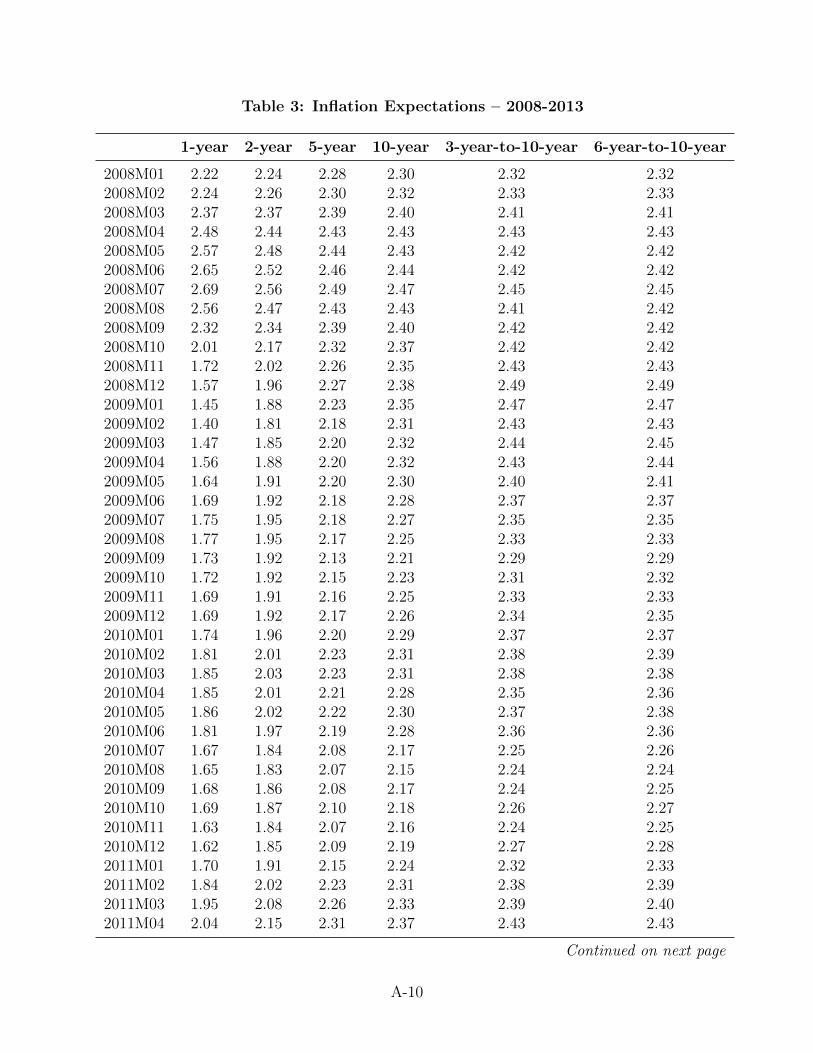
Table 3: Inflation Expectations – 2008-2013

1-year 2-year 5-year 10-year 3-year-to-10-year 6-year-to-10-year

2008M01 2.22 2.24 2.28 2.30 2.32 2.322008M02 2.24 2.26 2.30 2.32 2.33 2.332008M03 2.37 2.37 2.39 2.40 2.41 2.412008M04 2.48 2.44 2.43 2.43 2.43 2.432008M05 2.57 2.48 2.44 2.43 2.42 2.422008M06 2.65 2.52 2.46 2.44 2.42 2.422008M07 2.69 2.56 2.49 2.47 2.45 2.452008M08 2.56 2.47 2.43 2.43 2.41 2.422008M09 2.32 2.34 2.39 2.40 2.42 2.422008M10 2.01 2.17 2.32 2.37 2.42 2.422008M11 1.72 2.02 2.26 2.35 2.43 2.432008M12 1.57 1.96 2.27 2.38 2.49 2.492009M01 1.45 1.88 2.23 2.35 2.47 2.472009M02 1.40 1.81 2.18 2.31 2.43 2.432009M03 1.47 1.85 2.20 2.32 2.44 2.452009M04 1.56 1.88 2.20 2.32 2.43 2.442009M05 1.64 1.91 2.20 2.30 2.40 2.412009M06 1.69 1.92 2.18 2.28 2.37 2.372009M07 1.75 1.95 2.18 2.27 2.35 2.352009M08 1.77 1.95 2.17 2.25 2.33 2.332009M09 1.73 1.92 2.13 2.21 2.29 2.292009M10 1.72 1.92 2.15 2.23 2.31 2.322009M11 1.69 1.91 2.16 2.25 2.33 2.332009M12 1.69 1.92 2.17 2.26 2.34 2.352010M01 1.74 1.96 2.20 2.29 2.37 2.372010M02 1.81 2.01 2.23 2.31 2.38 2.392010M03 1.85 2.03 2.23 2.31 2.38 2.382010M04 1.85 2.01 2.21 2.28 2.35 2.362010M05 1.86 2.02 2.22 2.30 2.37 2.382010M06 1.81 1.97 2.19 2.28 2.36 2.362010M07 1.67 1.84 2.08 2.17 2.25 2.262010M08 1.65 1.83 2.07 2.15 2.24 2.242010M09 1.68 1.86 2.08 2.17 2.24 2.252010M10 1.69 1.87 2.10 2.18 2.26 2.272010M11 1.63 1.84 2.07 2.16 2.24 2.252010M12 1.62 1.85 2.09 2.19 2.27 2.282011M01 1.70 1.91 2.15 2.24 2.32 2.332011M02 1.84 2.02 2.23 2.31 2.38 2.392011M03 1.95 2.08 2.26 2.33 2.39 2.402011M04 2.04 2.15 2.31 2.37 2.43 2.43

Continued on next page

A-10

Table 3 – Inflation Expectations, 2008–2013 (continued)

1-year 2-year 5-year 10-year 3-year-to-10-year 6-year-to-10-year

2011M05 2.07 2.17 2.31 2.37 2.42 2.432011M06 2.08 2.17 2.30 2.36 2.40 2.412011M07 2.17 2.26 2.38 2.43 2.48 2.482011M08 2.14 2.24 2.36 2.41 2.46 2.462011M09 2.04 2.16 2.29 2.35 2.39 2.402011M10 2.01 2.14 2.29 2.34 2.39 2.402011M11 1.99 2.12 2.28 2.34 2.39 2.392011M12 1.96 2.11 2.27 2.33 2.38 2.392012M01 1.97 2.11 2.27 2.33 2.38 2.382012M02 2.07 2.18 2.31 2.36 2.41 2.422012M03 2.13 2.21 2.32 2.36 2.40 2.412012M04 2.16 2.22 2.32 2.35 2.39 2.392012M05 2.12 2.19 2.29 2.33 2.37 2.382012M06 2.07 2.17 2.29 2.34 2.38 2.392012M07 2.03 2.15 2.29 2.34 2.39 2.392012M08 2.03 2.18 2.32 2.37 2.42 2.422012M09 2.03 2.18 2.31 2.36 2.41 2.412012M10 2.02 2.17 2.30 2.35 2.39 2.392012M11 2.03 2.18 2.31 2.35 2.39 2.402012M12 2.05 2.18 2.31 2.35 2.40 2.402013M01 2.04 2.16 2.29 2.34 2.38 2.382013M02 2.05 2.16 2.28 2.33 2.37 2.382013M03 2.08 2.17 2.29 2.34 2.38 2.382013M04 2.10 2.18 2.30 2.35 2.39 2.392013M05 2.07 2.15 2.28 2.33 2.37 2.372013M06 2.04 2.15 2.28 2.34 2.39 2.392013M07 1.99 2.12 2.27 2.33 2.38 2.39

A-11

Table 4: Real Interest Rates, 2008–2013

6-month 1-year 2-year 5-year 10-year

2008M01 0.63 0.36 0.19 0.70 1.662008M02 -0.15 -0.31 -0.30 0.54 1.712008M03 -0.81 -0.84 -0.75 0.09 1.432008M04 -0.85 -0.69 -0.42 0.40 1.532008M05 -0.77 -0.49 -0.10 0.75 1.712008M06 -0.58 -0.24 0.20 1.03 1.902008M07 -0.76 -0.43 -0.02 0.83 1.772008M08 -0.65 -0.41 -0.08 0.70 1.692008M09 -0.48 -0.42 -0.27 0.48 1.562008M10 -0.32 -0.57 -0.64 0.45 2.032008M11 -0.21 -0.69 -0.97 0.09 1.852008M12 -0.61 -1.07 -1.36 -0.68 0.662009M01 -0.60 -0.98 -1.21 -0.52 0.822009M02 -0.43 -0.74 -0.91 -0.16 1.202009M03 -0.57 -0.80 -0.92 -0.25 1.032009M04 -0.86 -0.96 -0.97 -0.24 1.042009M05 -1.08 -1.10 -0.98 0.01 1.452009M06 -1.24 -1.08 -0.73 0.53 1.902009M07 -1.34 -1.22 -0.91 0.32 1.732009M08 -1.41 -1.22 -0.83 0.43 1.742009M09 -1.40 -1.27 -0.95 0.27 1.582009M10 -1.42 -1.28 -0.96 0.21 1.512009M11 -1.39 -1.34 -1.09 0.10 1.522009M12 -1.29 -1.26 -1.03 0.19 1.662010M01 -1.41 -1.33 -1.02 0.30 1.742010M02 -1.48 -1.42 -1.14 0.17 1.682010M03 -1.53 -1.40 -1.06 0.24 1.682010M04 -1.52 -1.35 -0.95 0.41 1.782010M05 -1.50 -1.41 -1.16 0.02 1.372010M06 -1.44 -1.40 -1.22 -0.13 1.182010M07 -1.31 -1.31 -1.22 -0.26 1.082010M08 -1.28 -1.33 -1.32 -0.55 0.732010M09 -1.29 -1.36 -1.37 -0.60 0.692010M10 -1.28 -1.41 -1.51 -0.84 0.552010M11 -1.22 -1.32 -1.38 -0.68 0.782010M12 -1.18 -1.28 -1.21 -0.14 1.332011M01 -1.28 -1.38 -1.29 -0.15 1.362011M02 -1.50 -1.48 -1.23 0.04 1.462011M03 -1.66 -1.62 -1.38 -0.13 1.282011M04 -1.82 -1.72 -1.41 -0.12 1.28

Continued on next page

A-12

Table 4 – Real Interest Rates – 2008-2013 (continued)

6-month 1-year 2-year 5-year 10-year

2011M05 -1.89 -1.82 -1.60 -0.46 0.992011M06 -1.84 -1.83 -1.72 -0.71 0.842011M07 -1.90 -1.91 -1.81 -0.82 0.782011M08 -1.87 -1.95 -1.97 -1.30 0.052011M09 -1.80 -1.87 -1.90 -1.36 -0.232011M10 -1.75 -1.81 -1.81 -1.18 -0.052011M11 -1.70 -1.80 -1.84 -1.31 -0.212011M12 -1.68 -1.77 -1.82 -1.32 -0.242012M01 -1.70 -1.79 -1.85 -1.36 -0.262012M02 -1.77 -1.83 -1.87 -1.42 -0.312012M03 -1.87 -1.86 -1.82 -1.23 -0.082012M04 -1.90 -1.89 -1.87 -1.35 -0.212012M05 -1.85 -1.85 -1.86 -1.46 -0.472012M06 -1.77 -1.80 -1.82 -1.50 -0.672012M07 -1.69 -1.77 -1.86 -1.60 -0.772012M08 -1.66 -1.78 -1.88 -1.54 -0.622012M09 -1.63 -1.78 -1.90 -1.57 -0.582012M10 -1.60 -1.76 -1.86 -1.52 -0.562012M11 -1.63 -1.78 -1.88 -1.57 -0.662012M12 -1.68 -1.81 -1.89 -1.54 -0.592013M01 -1.73 -1.82 -1.87 -1.42 -0.362013M02 -1.77 -1.83 -1.86 -1.39 -0.282013M03 -1.82 -1.86 -1.88 -1.42 -0.312013M04 -1.88 -1.90 -1.92 -1.54 -0.542013M05 -1.87 -1.87 -1.86 -1.39 -0.332013M06 -1.83 -1.83 -1.76 -1.06 0.072013M07 -1.75 -1.80 -1.70 -0.81 0.38

A-13