temporal mapping of phytoplankton assemblages in lake geneva: annual and interannual changes in...

Temporal Mapping of Phytoplankton Assemblages in Lake Geneva: Annual and InterannualChanges in Their Patterns of SuccessionAuthor(s): Orlane Anneville, Sami Souissi, Frédéric Ibanez, Vincent Ginot, Jean Claude Druartand Nadine AngeliSource: Limnology and Oceanography, Vol. 47, No. 5 (Sep., 2002), pp. 1355-1366Published by: American Society of Limnology and OceanographyStable URL: http://www.jstor.org/stable/3068955 .

Accessed: 14/06/2014 12:32

Your use of the JSTOR archive indicates your acceptance of the Terms & Conditions of Use, available at .http://www.jstor.org/page/info/about/policies/terms.jsp

.JSTOR is a not-for-profit service that helps scholars, researchers, and students discover, use, and build upon a wide range ofcontent in a trusted digital archive. We use information technology and tools to increase productivity and facilitate new formsof scholarship. For more information about JSTOR, please contact [email protected].

.

American Society of Limnology and Oceanography is collaborating with JSTOR to digitize, preserve andextend access to Limnology and Oceanography.

http://www.jstor.org

This content downloaded from 195.34.79.253 on Sat, 14 Jun 2014 12:32:30 PMAll use subject to JSTOR Terms and Conditions

http://www.jstor.org/action/showPublisher?publisherCode=limnoc

http://www.jstor.org/stable/3068955?origin=JSTOR-pdf

http://www.jstor.org/page/info/about/policies/terms.jsp


Limnol. Oceunogr., 47(5), 2002, 1355-1366 ((3 2002, by the American Society of Limnology and Oceanography, Inc.

Temporal mapping of phytoplankton assemblages in Lake Geneva: Annual and interannual changes in their patterns of succession

Orlane Annevillel INRA, Station d'Hydrobiologie Lacustre, BP 511, 74203 Thonon-les-Bains Cedex, France

Sami Souissi Ecosystem Complexity Research Group, Station Marine de Wimereux, Universite des Sciences et Technologies de Lille, CNRS-UMR 8013 ELICO, 28 avenue Foch, BP 80, 62930 Wimereux, France

Frederic Ibanez Laboratoire d'Oceanographie de Villefranche. LOV-UMR 7093, Station Zoologique BP 28, 06230 Villefranche-sur-Mer, France

Vincent Ginot INRA, Unite de biometrie. Domaine St-Paul, 84914 Avignon, Cedex 9, France

Jean Claude Druart and Nadine Angeli INRA, Station d'Hydrobiologie Lacustre, BP 511, 74203 Thonon-les-Bains Cedex, France

Abstract The implementation of a conservation program since the early 1980s resulted in a reduction in phosphorus

concentrations in Lake Geneva. However, in the l990s, phytoplankton biomass increased again, almost reaching the high values recorded during the period of greatest P loading. The structural changes in the phytoplankton of Lake Geneva over the past 25 yr have been analyzed using a recently developed statistical method based on hierarchical clustering and Bayesian probabilities. This method has been used to identify phytoplankton assemblages and to map annual and interannual successional patterns simultaneously. Characteristic species were identified for each cluster after calculation of their relative species fidelity and specificity indices. Six distinct phytoplankton assemblages were identified, and although the way species are organized into communities remains unclear, the seasonal patterns of succession are consistent with the C-S-R adaptive strategies and are characteristic of temperate lakes. This pattern broadly recurred over the years, but was markedly influenced by both human activity and regional climatic changes: The warmer winters and springs recorded in Europe since 1988 led to an earlier clear-water phase. In the l990s, the earlier and deeper depletion of dissolved inorganic phosphorus led to colonization in the summer by large species tolerant of low light levels and that could develop deeper in the water column, where phosphorus was still abundant. Their size made them less vulnerable to grazing losses, which favors their accumulation and lead to an unexpected high biomass in recent years.

Lale Geneva (46°27'N, 6°32'E) has a volume of 89 km3,

which makes it the greatest freshwater reserve in Western Europe. It is used for professional and leisure fishing and is a center for tourism. Like many other water bodies in in- dustrialized countries, Lake Geneva switched rapidly from being oligotrophic to mesotrophic during the 1960s when, because of the expansion of human activities in its catchment area, its mean annual total phosphorus concentration sud-

l Present address: Universitat Konstanz, D-78457 Konstanz, Ger- many

Acknowledgments We are indebted to everyone who has contributed to the elabo-

ration of the Lake Geneva data set over the past 25 yr. We also thank M. Ghosh and K. Ghertsos for checking the English. This research project was part of 0. Anneville's doctoral dissertation and was funded by the International Committee for the Protection of the Water of Lake Geneva (CIPEL), the French Ministry of Envi- ronment, and GIP HydroSystemes.

denly increased within a few years from 10 ,ug P L-' to 40 ,ug P L-1. In the 1970s, the economic importance of the lake made it necessary to reduce phosphorus loading and develop a monitoring program that is still in action (CIPEL: Inter- national Committee for the Protection of the water of Lake Geneva). In the early 1980s, the phosphorus concentration responded to the reduction in P loading, and mean annual concentrations in total phosphorus fell from a maximum of 89.5 ,ug P L-1 in 1979 to 39.6 ,ug P L-1 in 1998. Despite this reduction, the change in phytoplankton biomass proved more chaotic than expected and recently even began to increase (Anneville and Pelletier 2000). Paradoxical relationships between phosphorus and phytoplankton trends are not peculiar to Lake Geneva, and there is often a considerable time lag before obtaining any response to a decrease in a nutrient (Sas 1989; Carpenter and Cottingham 1997). In a context of lake management, this time lag makes it difficult to decide how best to implement expensive programs of restoration and highlights the necessity for a better understand-

1355



Q N 0 ztwto r'te pv x ;! w

gg46°25'- 7mt

<& \ Dranse , ' \Rhone

r r s\+ Largelah _ +,/' q< S9mall lake

Geneve - -t 6°10' 6°30' 6°50'

Longitude

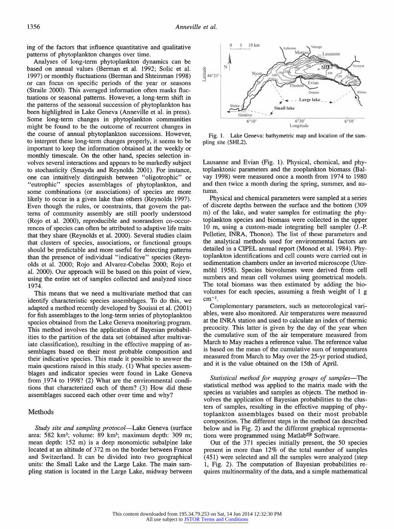
Fig. 1. Lake Geneva: bathymetric map and location of the sampling site (SHL2).

Lausanne and Evian (Fig. 1). Physical, chemical, and phy- toplanktonic parameters and the zooplankton biomass (Bal- vay 1998) were measured once a month from 1974 to 1980 and then twice a month during the spring, summer, and au- tumn.

Physical and chemical parameters were sampled at a series of discrete depths between the surface and the bottom (309 m) of the lake, and water samples for estimating the phytoplankton species and biomass were collected in the upper 10 m, using a custom-made integrating bell sampler (J.-P. Pelletier, INRA, Thonon). The list of these parameters and the analytical methods used for environmental factors are detailed in a CIPEL annual report (Monod et al. 1984). Phy- toplankton identifications and cell counts were carried out in sedimentation chambers under an inverted microscope (Uter- mohl 1958). Species biovolumes were derived from cell numbers and mean cell volumes using geometrical models. The total biomass was then estimated by adding the biovolumes for each species, assuming a fresh weight of 1 g cm-3.

Complementary parameters, such as meteorological variables, were also monitored. Air temperatures were measured at the INRA station and used to calculate an index of thermic precocity. This latter is given by the day of the year when the cumulative sum of the air temperature measured from March to May reaches a reference value. The reference value is based on the mean of the cumulative sum of temperatures measured from March to May over the 25-yr period studied, and it is the value obtained on the l5th of April.

Statistical method for mapping groups of samples-The statistical method was applied to the matrix made with the species as variables and samples as objects. The method involves the application of Bayesian probabilities to the clusters of samples, resulting in the effective mapping of phytoplankton assemblages based on their most probable composition. The different steps in the method (as described below and in Fig. 2) and the different graphical representa- tions were programmed using Matlab62' Software.

Out of the 371 species initially present, the 50 species present in more than 12% of the tctal number of samples (451) were selected and all the samples were analyzed (step 1, Fig. 2). The computation of Bayesian probabilities re- quires multinormality of the data, and a simple mathematical

1356 Anneville et al.

ing of the factors that influence quantitative and qualitative patterns of phytoplankton changes over time.

Analyses of long-term phytoplankton dynamics can be based on annual values (Berman et al. 1992; Solic et al. 1997) or monthly fluctuations (Berman and Shteinman 1998) or can focus on specific periods of the year or seasons (Straile 2000). This averaged information often masks fluctuations or seasonal patterns. However, a long-term shift in the patterns of the seasonal succession of phytoplankton has been highlighted in Lake Geneva (Anneville et al. in press). Some long-term changes in phytoplankton communities might be found to be the outcome of recurrent changes in the course of annual phytoplankton successions. However, to interpret these long-term changes properly, it seems to be important to keep the information obtained at the weekly or monthly timescale. On the other hand, species selection involves several interactions and appears to be markedly subject to stochasticity (Smayda and Reynolds 2001). For instance, one can intuitively distinguish between "oligotrophic" or "eutrophic" species assemblages of phytoplankton, and some combinations (or associations) of species are more likely to occur in a given lake than others (Reynolds 1997). Even though the rules, or constraints, that govern the patterns of community assembly are still poorly understood (Rojo et al. 2000), reproducible and nonrandom co-occurrences of species can often be attributed to adaptive life traits that they share (Reynolds et al. 2000). Several studies claim that clusters of species, associations, or functional groups should be predictable and more useful for detecting patterns than the presence of individual "indicative" species (Reyn- olds et al. 2000; Rojo and Alvarez-Cobelas 2000; Rojo et al. 2000). Our approach will be based on this point of view, using the entire set of samples collected and analyzed since 1974.

This means that we need a multivariate method that can identify characteristic species assemblages. To do this, we adapted a method recently developed by Souissi et al. (2001) for fish assemblages to the long-term series of phytoplankton species obtained from the Lake Geneva monitoring program. This method involves the application of Bayesian probabilities to the partition of the data set (obtained after multivariate classification), resulting in the effective mapping of assemblages based on their most probable composition and their indicative species. This made it possible to answer the main questions raised in this study. (1) What species assemblages and indicator species were found in Lake Geneva from 1974 to 1998? (2) What are the environmental conditions that characterized each of them? (3) How did these assemblages succeed each other over time and why?

Methods

Study site and sampling protocol-Lake Geneva (surface area: 582 km2; volume: 89 km3; maximum depth: 309 m; mean depth: 152 m) is a deep monomictic subalpine lake located at an altitude of 372 m on the border between France and Switzerland. It can be divided into two geographical units: the Small Lake and the Large Lake. The main sampling station is located in the Large Lake, midway between



Species

X(nrx)

Stepla: Species

Phytoplankton assemblages in Lake Geneva 1357

transformation (e.g., log, log-log) was not sufficient for this purpose; consequently, a principal component analysis (PCA) was applied to the log-transformed data (step lb, Fig. 2). Successive combinations of the first components account- ing for more than 90% of total variance were then retained to test the multinormality by the Dagnelie method (Legendre and Legendre 1998; Souissi et al. 2001).

In the second step (Fig. 2), a hierarchical classification was applied to the PCA scores (matrix A'), using the Eu- clidean distance and clustering strategy of flexible links with beta = -0.25 (Legendre and Legendre 1998) to achieve the effective separation into groups for the subsequent mapping. This technique and its subsequent treatment are detailed in Souissi et al. (2001), where detailed mathematical represen- tations can be found. Essentially, the dendrogram can be used for different resolutions to be obtained from the data set depending on the choice of cutoff level. In this case, only one hierarchical level was taken into consideration. This is thought to provide optimal mapping for the ecological interpretation of the clusters.

After this, the third step consists of calculating the probability that each sample belongs to each of the clusters defined above (Harff et al. 1993). This calculation is based on a Bayesian conditional probability: each object (one sample) Oi is a q'-dimensional variable, where q' is the number of the selected PCA axes (A' in Fig. 2).

°i = {Xi,l, Xi,2 * * * } Xi,q} (1)

xij is the score of sample i according to the axis j. Depending on the scores of each object Oi, the probability

that it belongs to a cluster Gj is expressed by Bayes relationship (Harff et al. 1993).

p; 1 l 1/2eXp(-dj2(i)/2)

P(O, E Gj) = g E Pk | | exp(-dk2(i)12) k=l k

(2)

pj is an a priori probability that only represents the propor- tion of the number of samples in the cluster Gj to the total number of samples (451), and d2(i) is the generalized Ma- halanobis' distance between Gj and Oi

d2(i) = (°i - mG) E (°i - mJG) (3)

where mjG is the centroid of the cluster Gj, that is, the data point (vector) tha is the mean of the scores for the principal axes in the dimenJlon of samples.

Assuming that the dispersion matrices are equal (Harff and Davis 1990),

E = E = E V i,j E {1,2,...,g} i j o

a pooled variance-covariance matrix Ep (Cooley and Lohnes 1971; Legendre and Legendre 1998) was used as a substitute for the normal dispersion matrix E in computing d2.

When the maximum value of the conditional probability of a sample was obtained for another cluster, the samples were reallocated. New clusters were then obtained, and the procedure was repeated until the composition of the clusters

Fig. 2. Flowchart of the statistical method, which can be sum- marized as consisting of four major steps: (1) species selection, (2) hierarchical classification of samples, (3) computation of conditional probabilities and reallocation of samples, and (4) mapping of groups of samples.



Table 1. Comparison of group average probabilities calculated before and after the reallocation.

No. of Mean SD samples

Group I Before 0.81 0.18 64 After 0.88 0.11 79

Group II Before 0.77 0.25 104 After 0.85 0.14 83

Group III Before 0.75 0.22 63 After 0.84 0.14 99

Group IV Before 0.73 0.32 47 After 0.88 0.16 36

Group V Before 0.73 0.27 77 After 0.82 0.17 70

Group VI Before 0.73 0.33 55 After 0.91 0.10 41

Group VII Before 0.81 0.22 41 After 0.86 0.14 43


c)

a, 3C ._

._, 4C -

L;

70 -

Fig. 3. Dendrogram showing the result of the hierarchical clustering and the selected hierarchical level thought to give the optimal distribution for the ecological interpretation of the clusters. Characterization of the environmental conditions To

characterize the environmental conditions associated with each cluster of samples obtained by the previous method, we used the box-and-whiskers plots representation, which sum- marized the distribution of values. Among the set of recorded environmental factors, we retained the Secchi depth; herbivorous zooplankton biomass; mean weighted values recorded in the O-10-m layer (the layer where phytoplankton is sampled) for temperature, dissolved inorganic nitrogen (DIN; ,ug N L-l), and dissolved inorganic phosphorus (DIP; ,ug P L-l); and silicates (mg SiO2 L-l). We also determined the depths of the DIP-depleted layer, which is the greatest depth at which the dissolved inorganic phosphorus falls below 10 ,ug P L-l and is thus likely to become critical for algae growth (Sas 1989).

Results

Cluster analysis and reallocation of samples The hierarchical classification of samples produced the dendrogram shown in Fig. 3. The level resulting in seven coherent groups of samples was chosen (Fig. 3). Table 1 shows that the reallocation of samples improved the average probability for any sample to be a member of its cluster and reduced the dispersion (standard deviation) around this value. This means that the intragroup homogeneity was improved after reallocation.

Distribution of samples into groups: evidence of seasonal dynamics The conditional probabilities of samples can be used to estimate the monthly average probabilities associated with each of the seven groups (Fig. 4). The distribution obtained corresponds to a seasonal pattern. Group I shows strong average probabilities for all the winter months. All the samples in Group II preferentially occurred during the period ranging from March to June, with the highest probabilities for April and May. Every month had a high probability for Group III; however, the highest probability was found for June. In the case of Group IV, higher probabilities were restricted to the early summer, and in particular to July.

remained stable. The obtained final partition called the "final partition groups of samples" was then considered for the rest of the analysis.

The next step consists of mapping the groups of samples (Fig. 2). To do this, the time series of the conditional probabilities were interpolated (Pg, Fig. 2) at regular daily steps, which gave an estimation of a vector of conditional probabilities p, for any given date (t) between 1974 and 1998.

p, = { p,( 1 ), p,(2), . . ., p,(g) lt (4)

The date, t, is considered to belong to the assemblage j representing the group of samples j if its probability pt(j) is greatest for group j. Maps were then created using different levels of grey to denote the different groups identified after interpolation. The map showed the monthly variations versus years (Fig. 2). The final map was not very sensitive to the interpolation algorithm (spline, linear, . . .).

Characterization of species assemblages and species associations After mapping the groups of samples, the species characterizing each partition were further identified using the indicator value index proposed by Dufrene and Legendre (1997). This indicator index is obtained by mul- tiplying by 100 the product of two independently computed values: the specificity (SPjX) and fidelity (FIjs) of a species, s, toward a group of samples, Gj.

SPj, = NIj ,lNI+j FIjX-NSjslNSjH

NIjs is the mean biomass of species s across the samples pertaining to Gj, NI+j is the sum of the mean biomass of species s within the various groups in the partition, NSj,s is the number of samples in Gj where species s is present, and NIj+ is the total number of samples in that group. The specificity of a species for a group is therefore greatest if this species is present only in this group, whereas the fidelity of a species to a group is greatest if this species is present in all samples of the group considered.




1.0

0.8

0.6

0.4

0.2

0.0

For Group V, high probabilities were found for all the summer months from July to September. Groups VI and VII had high probabilities for the second half of the year, with the highest values from August to November and from Septem- ber to December, respectively.

Indicator species detected for each group of samples: evidence for the occurrence of phytoplankton assemblages- Indicator value indices for phytoplankton species were computed for the seven groups. Apart from the species Planktothrix rubescens, for which the indicator value fell from 57 to 51, the indicative power of species was shown to increase after reallocating the samples. For example, the indicator value obtained after cluster analysis for Stephan- odiscus neoastraea, Stephanodiscus minutulus, Chlamydo- monas conica v. subconica, Dinobryon sociale, and Diatoma tenuis were 59, 82, 32, 45, and 79%, respectively, whereas they were 74, 83, 61, 53, and 96% after reallocation (Table 2). Table 2 summarizes the species with an indicator value above the arbitrary threshold of 25%. High indicator values mean that the species did not occur randomly. The groups of species listed in Table 2 can therefore be considered to be distinct "phytoplankton assemblages."

A single characteristic indicator species was found for Group I (the diatom S. neoastraea), and the indicator species for Group II were mainly individual cells and nanoplankton forms. The most representative species making up an association (with a fidelity value close to 100%) were the diatom S. minutulus, the Cryptophycean Rhodomonas minuta, and the Chlorophycean Chlorella vulgaris. Group III had no indicator species; it simply consisted of samples with species compositions that differed from those of the other groups and could, therefore, be considered to be a "residual" group that is not associated with any characteristic species assemblage. Group IV was characterized by the nanoplankton Chlorophycean C. conica v. subconica and by microplankton species such as Peridinium willei, Staurastrum cingulum, and Cosmarium depressum v. planctonicum. This group was also characterized by the co-occurrence of Asterionella formosa and Cryptomonas (Fidelity index = 100%). The indicators of Group V were mostly mixotrophic microplankton (D. sociale, Ceratium hirundinella) or motile species (D. sociale, C. hirundinella, Phacotus lendneri). Group VI was characterized by large forms (less vulnerable to grazing losses), and most of the species were not motile, unicellular elongated, or filamentous. The Group VI species with the greatest indicator value was D. tenuis, and with the conjugate Mougeotia gracillima, this made up an association peculiar to this group (with fidelity values of 100 and 81%, respectively). The cyanobacterium Oscillatoria limnetica was also found to have a high indicative value for this group and a rather high probability of co-occurrence with the two previous species (fidelity index of 68%). The indicator species for the seventh group were all microplankton, and most of them consisted of poorly edible filamentous forms. The most characteristic species in this last group were the cyanobacterium P. rubescens and Chrysophycean Mallomonas acaroides, both of which can regulate their vertical position in the water column. In contrast, the other two species characteristic of this group, the diatoms Stephanodiscus binder-

1.0

0.8

0.6

0.4

0.2

0.0

1.0

0.8

0.6

0.4

0.2

0.0

1.0

0.8

0.6

0.4

0.2

0.0

1.0

0.8

0.6

0.4

0.2

0.0

1.0

0.8

0.6

0.4

0.2

0.0

* - 4

* - 4

o

a)

'e

1.0

0.8

0.6

0.4

0.2

0.0

v S ¢ 2 D Y ¢ m o z Q

Month Fig. 4. Histograms of monthly average probabilities recorded

for each of the seven selected groups.



Table 2. List of the indicator species recorded in the seven groups of samples. The following characteristics are specified in the table: IndVal(Fidelity), the indicator value and the fidelity value; GrTax, the taxonomic group (Cya, cyanophyte; Din, dinoflagellate; Cry, cryp- tophyte; Chr, chrysophyte; Dia, diatom; Chl, chlorophyte; Con, conjugate); Cat., the morphological category (i, individual cell; c, colonial; f, filamentous); size (M, microplankton; Na, nanoplankton); and information about the edibility, motility, and mixotrophy.

IndVal Assemblage (Fidelity) GrTax Cat. Size Edibility Motility Mixotrophy

31(66)

28(50)

26(6 1)


Group I Stephanodiscus neoastraea

Hakansson et Hickel Group II

Stephanodiscus minutulus (Kutzing) Cleve et Moller

Rhodomonas minuta Skuja

Chlorella vulgaris Beij

Gymnodinium lantzschii Utermohl

Gymnodinium helveticum Penard

Rhodomonas minuta v. nann. Skuja

Aulacoseira islandica su. helvetica (O. F. Muller) Simonsen

Stephanodiscus alpinus Hustedt

Hyaloraphidium contortum Pasch. et Kors

Asterionella formosa Hassal

Group III

74( 100)

83(95)

59(94)

53(74)

49(7 1)

44(92)

43(100)

36(52)

35(46)

30(47)

25(88)

Dia

Dia

Cry

Chl

Din

Din

Cry

Dia

Dia

Chl

i M Yes No

i Na Yes No

i Na Yes Yes

i Na Yes No

i Na Yes Yes

i M Yes Yes

i Na Yes Yes

f M No

i Na Yes No

i M Yes No

Dia M No No

Group IV Chlamydomonas conica v. subconica

(Starm.) Ettl. Peridinium willei

Huitfeldt-Kaas Staurastrum cingulum

(W. et G. S. West) G. M. Smith Cosmarium depressum v. p.

Reverdun Asterionella formosa

Hassal Staurastrum sebaldii v. o.

(Lutkem) Teil Oocystis lacustris

Chodat Sphaerocystis schroeteri

Chodat Cryptomonas sp. Oocystis solitaria

Wittr. in Wittr. et Nordst. Group V

Dinobryon sociale Ehr.

Ceratium hirundinella (O. F. Muller) Bergh.

Phacotus lendneri Chodat

Aphanothece clathrata v. rosea Skuja

Nitzschia acicularis W. Smith

61(64)

50(69)

39(69)

38(58)

36(100)

35(58)

Chl

Din

Con

Con

Dia

Con

Chl

i Na Yes Yes

i M Yes Yes

i M No No

i M Yes No

c M No No

i M No No

c M Yes

c M Yes i M Yes

No

30(42)

30(58) Chl 29( 100) Cry

27(47)

Yes Yes Yes

Chl i Na Yes No

53(7 1)

49(97)

Chr c M No Yes Yes

Din

Chl

Cya

Dia

i M Yes Yes Yes

i Na Yes Yes

c M No No

i M Yes No



Table 2. Continued.

IndVal Assemblage (Fidelity) GrTax Cat. Size Edibility Motility Mixotrophy

Aphanizomenon fftos aquae (L.) Ralfs 25(63) Cya f M No No

Group VI Diatoma tenuis

Agardhii 96(100) Dia i M No No Mougeotia gracillima

(Hass.) Witkock 61(81) Con f M No No Oscillatoria limnetica

Lemm. 59(68) Cya f M No Yes Fragilaria ulna v. angustissima

(Nitzsch) Lange Bertalot 26(63) Dia i M No No Group VII

Planktothrix rubescens de Candolle 51(77) Cya f M No Yes

Mallomonas acaroides Perty 38(63) Chr i M Yes Yes

Stephanodiscus binderanus (Kutzing) Krieger 34(58) Dia f M No

Aulacoseira granulata v. ang. (O. F. Muller) Simonsen 26(44) Dia f M No No


anus and Aulacoseira granulata v. angustissima, are not motile.

Characterization of the "environmental template" associated with the seven groups of samples Figure S shows the patterns of environmental parameters within the seven groups of samples. Groups IV-VI displayed a narrow range of variation for dissolved inorganic phosphorus concentrations. Group I was characterized by low zooplankton biomass, high nutrient concentrations, and low water temperatures that corresponds to the usual winter conditions in temperate European deep lakes. Group II differed slightly from Group I by having lower water transparency (Fig. SA) and nutrient concentration (Fig. SC-E) values. In Group II, zooplankton biomass was higher than in Group I (Fig. SF). Group III was associated with good transparency (Fig. SA), intermediate water temperature (Fig. SB) and nutrient concentrations (Fig. SC-E), and high zooplankton biomass (Fig. SF). The environmental patterns of Group IV were similar to those of Groups V and VI, apart from having a higher concentration of silicates and a higher biomass of herbivorous zooplankton. These three groups were all characterized by warmer water, roughly ranging from 16 to 20°C (Fig. SB), and very low nutrient concentrations in the top 10 m. Nitro- gen and dissolved inorganic phosphorus concentrations were less than 300 ,ug N L-l and 10 ,ug P L-l, respectively. Group VI differed from the other groups on the basis of the depth of the DIP-depleted layer. In contrast to Groups IV and V, it was always associated with a DIP-depleted layer extending to a depth of more than 30 m (Fig. 6). Group VII consisted of samples characterized by lower water temperatures, ranging from 10 to 16°C, and higher nutrient concentrations than were found for the samples of the three previous groups (0.30 to 1 mg Si L-' for the silicates, lS0-375 ,ug N L-' for nitrogen, and S-10 ,ug P L-' for phosphorus).

o I II III IV V VI VII 4

I II III IV V VI VII

-

o-

ct

-

s

o cT

I II III IV V VI VII Group

I II III IV V VI VII Group

Fig. 5. Box-and-whisker plots describing the distributions of the herbivorous zooplankton biomass and the physical and chemical descriptors within each of the seven selected groups. The horizontal lines across the boxes correspond to the lower quartile, median, and upper quartile values. The notches in the box show the 95% con- fidence interval of the median. When the notches between boxes did not overlap, the medians were considered to be significantly different. The whiskers are lines extending from each end of the box to show the extent of the rest of the data.

T A

18

E 15

g

6 ' ; tr f f t f 3

22 20

U 18 16

g 14 212

A 10

8 6

- | l

= 12

CL




98

96

94

92

90

88

86

84

82

80

78

76

74

* * * n

* * * *

* * * *

* * *

* * * *

* * * *

* * * *

* * * *

* * *

* * * *

* *

* * * *

* * * *

* * * *

* * *

* *

* * * *

* * * *

* * *

* * *

* * *

* * *

g * g

* * *

* * 5

* * {

* {W * * * *W-sa * * * sL_

* * * - * * _S-1 * * * * * |

* | | *

* |

* * |

* * * | * |

* * * * * |

* * * * * |

* * * | * |

* * * * * * |

* * * * * |

* * * * * |

* * |

* * |

* * |

* * |

* *

Group

fflVE

g VI

V

*E

I

* - * n - * - * n

*-n * n b * b

m _

_ * b

!S * | ._. * * |

* * |

* * |

* * -

p Oct Nov Dec * * - * * * * * * -

Jan Feb Mar Apr MiJr Jun Jul Aug Mod

_ 1 e,E'v,, 19..'g,-4'''

__ + + IA,, ,o ,atf ->o, A:vA fo F + . ... @ --' . - ' 9 '. ' \, 'i...

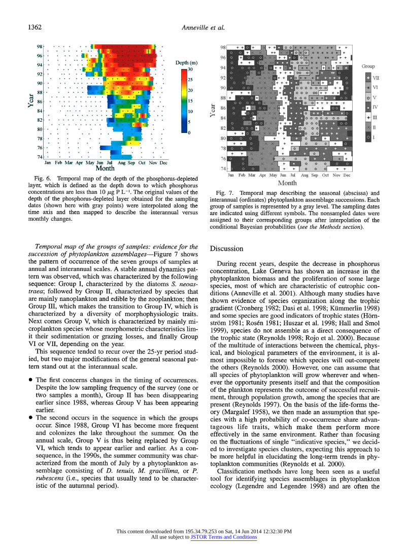
Jan Feb Mar Apr May Jun Jul Aug Sep Oct Nov Dec Fig. 6. Temporal map of the depth of the phosphorus-depleted

layer, which is defined as the depth down to which phosphorus concentrations are less than 10 ,ug P L-'. The original values of the depth of the phosphorus-depleted layer obtained for the sampling dates (shown here with gray points) were intexpolated along the time axis and then mapped to describe the interannual versus monthly changes.

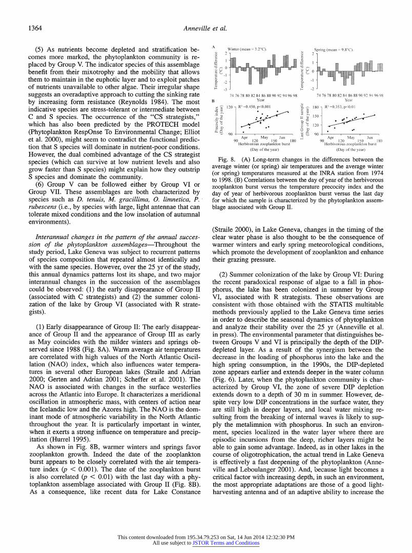
Temporal map of the groups of samples: evidence for the succession of phytoplankton assemblages Figure 7 shows the pattern of occurrence of the seven groups of samples at annual and interannual scales. A stable annual dynamics pattern was observed, which was characterized by the following sequence: Group I, characterized by the diatoms S. neoastraea; followed by Group II, characterized by species that are mainly nanoplankton and edible by the zooplankton; then Group III, which makes the transition to Group IV, which is characterized by a diversity of morphophysiologic traits. Next comes Group V, which is characterized by mainly microplankton species whose morphometric characteristics limit their sedimentation or grazing losses, and finally Group VI or VII, depending on the year.

This sequence tended to recur over the 25-yr period studied, but two major modifications of the general seasonal pattern stand out at the interannual scale.

* The first concerns changes in the timing of occurrences. Despite the low sampling frequency of the survey (one or two samples a month), Group II has been disappearing earlier since 1988, whereas Group V has been appearing earlier.

* The second occurs in the sequence in which the groups occur. Since 1988, Group VI has become more frequent and colonizes the lake throughout the summer. On the annual scale, Group V is thus being replaced by Group VI, which tends to appear earlier and earlier. As a consequence, in the 1990s, the summer community was characterized from the month of July by a phytoplankton assemblage consisting of D. tenuis, M. gracillima, or P. rubescens (i.e., species that usually tend to be characteristic of the autumnal period).

Month Fig. 7. Temporal map describing the seasonal (abscissa) and

interannual (ordinates) phytoplankton assemblage successions. Each group of samples is represented by a gray level. The sampling dates are indicated using different symbols. The nonsampled dates were assigned to their corresponding groups after intexpolation of the conditional Bayesian probabilities (see the Methods section).

Discussion

During recent years, despite the decrease in phosphorus concentration, Lake Geneva has shown an increase in the phytoplankton biomass and the proliferation of some large species, most of which are characteristic of eutrophic conditions (Anneville et al. 2001). Although many studies have shown evidence of species organization along the trophic gradient (Cronberg 1982; Dasi et al. 1998; Kummerlin 1998) and some species are good indicators of trophic states (Horn- strom 1981; Rosen 1981; Huszar et al. 1998; Hall and Smol 1999), species do not assemble as a direct consequence of the trophic state (Reynolds 1998; Rojo et al. 2000). Because of the multitude of interactions between the chemical, physical, and biological parameters of the environment, it is almost impossible to foresee which species will out-compete the others (Reynolds 2000). However, one can assume that all species of phytoplankton will grow wherever and when- ever the opportunity presents itself and that the composition of the plankton represents the outcome of successful recruit- ment, through population growth, among the species that are present (Reynolds 1997). On the basis of the life-forms theory (Margalef 1958), we then made an assumption that species with a high probability of co-occurrence share advan- tageous life traits, which make them perform more effectively in the same environment. Rather than focusing on the fluctuations of single "indicative species," we decid- ed to investigate species clusters, expecting this approach to be more helpful in elucidating the long-term trends in phytoplankton communities (Reynolds et al. 2000).

Classification methods have long been seen as a useful tool for identifying species assemblages in phytoplankton ecology (Legendre and Legendre 1998) and are often the

Dep (m) _30

25

-20 . .

^15

* t - 10 Q

* > *5

O




first step in unraveling the relationships between phytoplankton assemblages and environmental conditions (Fernandez and Bode 1994; Salmaso 1996). Often, large numbers of samples and the constraints imposed by the clustering strategy algorithm (here, a flexible link) can account for the presence of samples in a cluster with low conditional probabilities. The combination of a hierarchical classification with Bayesian probabilities is a novel way of assessing within- group heterogeneity (see Table 1). In this way, the reallocation of samples based on their maximal Bayesian probabilities produced a stable set of seven groups. Furthermore, from an ecological point of view, the indicative power of the species was greater after this reallocation. Finally, the identified sets of indicator species per group of samples make up "species assemblages" characterized by patterns in the occurrence of phytoplankton species. It is then possible to distinguish between co-occurring species (species with a high fidelity index) and species affiliated with an assemblage (species with a high specificity index). The patterns of these assemblages, therefore, relate to underlying ecological phe- nomena, as opposed to chance or accidental events.

The phytoplankton assemblages in Lake Geneva and their ecological significance Over the period investigated, the method characterized seven groups of samples and six phytoplankton assemblages (Table 2). Group III has no indicator species because the phytoplankton communities in the samples making up this group were not sufficiently similar or specific to identify species with high fidelity and specificity . < .

ndlces.

The phytoplankton assemblages are roughly homogeneous in terms of the morphological traits of their indicator species. The indicator species in Group II consisted mainly of unicellular nanoplankton forms, whereas filamentous microplankton species were more abundant in Groups VI and VII. This observation highlights the relationship between the morphological forms and "habitat properties" (Margalef 1958). Furthermore, depending on the functional traits of their indicator species, some assemblages could clearly be associated with the three primary adaptive strategies (C, competitor; S, stress-tolerant; R, disturbance-tolerant ruder- al), as adapted and applied by Reynolds (1980, 1984) to the aquatic environment. Group II, which is characterized by the association of invasive, small-sized species able to grow at low temperatures (S. minutulus, C. vulgaris, and R. minuta), can be likened to the typical C category. Group V is made up of S species, whose typical representative is C. hirundinella (Reynolds 1997), defined as intermediate between the C and S categories (Elliott et al. 2000), and intermediate species of the genera Dinobryon and Aphanizomenon, which also are recorded to span the C-S gaps (Reynolds 1997). Such species can be considered stress-tolerant competitors (CS), strategists that display strong growth rates and cold tolerance (as C strategists) but which benefit from their en- hanced ability to exploit and conserve nutrient resources. Groups VI and VII are characterized as containing R strategists, or genera and species able to tolerate low light inten- sities: D. tenuis, Mougeotia, Oscillatoria, P. rubescens, and Aulacoseira (Reynolds 1997).

The homogeneity of the distribution of species size and

adaptive strategy within each group is obvious, but it is not absolute. The best indicator species of Group IV (C. conica v. subconica) is a nanoplankton, whereas most of the others are microplankton. Furthermore, this assemblage presents various adaptive strategies. We also found genera belonging to the C (Chlamydomonas, Reynolds 1997), the S (P. willei, Reynolds 1997), and the R strategist categories (Asterionel- la, Elliot et al. 2000), as well as some intermediate C and S strategists (Sphaerocystis, Reynolds 1997). Thus, Group IV displays a high level of specific and functional diversity. In Group V, the best indicator species were colonial or unicellular, and although this group consisted mainly of microplankton, the nanoplankton species P. Iendneri had a high indicator value (Table 2). Because nanoplankton species occur in an assemblage dominated by microplankton, it is likely that some nanoplankton species are specialized as "un- dergrowth" in microplankton communities.

The general pattern of annual succession within phytoplankton assemblages in Lake Geneva The clustering was run without any temporal constraint, so the phytoplankton assemblages were not assumed to correspond to seasonal or interannual patterns of succession. Nevertheless, the succession of assemblages identified did reflect a strong seasonal pattern, and these seasonal changes in phytoplankton composition were greater than those detected between different years. This finding confirms the reproducible and recurrent character of seasonal changes in phytoplankton communities during the years studied (Reynolds 1984; Sommer 1986). In Lake Geneva, the seasonal succession of phytoplankton assemblage fits the following model.

(1) At the beginning of the year, the phytoplankton community is represented by an assemblage (Group I) characterized by S. neoastrae.

(2) In March-April, with the onset of the thermal stratification and a rise in temperature, a spring community (Group II) succeeds the winter community. The springtime development of phytoplankton is accompanied by a sharp fall in transparency and the increase in zooplankton (Fig. 5). This pioneer community can be expected to continue to ex- pand until it either runs out of nutrient or light energy or is checked by zooplankton grazing (Reynolds 1997), either of which could lead to a collapse of the phytoplankton biomass.

(3) In Lake Geneva, such a collapse occurs in June when herbivores reach high biomass. It is supposed to be mainly the result of zooplankton grazing and the decrease in SiO2 concentration (Gawler et al. 1986; Balvay 1998). It coincides with the emergence of Group III, a transition group between the spring community and the community that develops during the period of stratification.

(4) This is succeeded by Group IV, which is associated with high herbivorous biomass, high temperature, and ther- mocline-limiting exchanges between the euphotic and the richer aphotic layers. At the beginning of this seasonal step, when nutrients are still present, spatial structure acts syner- gistically with nutrient availability to favor the wide diversity of forms and functional properties. This is a pattern characteristic of the presummer community described by the Plankton Ecology Group (Sommer et al. 1986).




A (5) As nutnents become depleted and stratification becomes more marked, the phytoplankton community is replaced by Group V. The indicator species of this assemblage benefit from their mixotrophy and the mobility that allows them to maintain in the euphotic layer and to exploit patches of nutrients unavailable to other algae. Their irregular shape suggests an overadaptive approach to cutting the sinking rate by increasing form resistance (Reynolds 1984). The most indicative species are stress-tolerant or intermediate between C and S species. The occurrence of the "CS strategists," which has also been predicted by the PROTECH model (Phytoplankton RespOnse To Environmental Change; Elliot et al. 2000), might seem to contradict the functional predic- tion that S species will dominate in nutrient-poor conditions. However, the dual combined advantage of the CS strategist species (which can survive at low nutrient levels and also grow faster than S species) might explain how they outstrip S species and dominate the community.

(6) Group V can be followed either by Group VI or Group VII. These assemblages are both characterized by species such as D. tenuis, M. gracillima, O. Iimnetica, P. rubescens (i.e., by species with large, light antennae that can tolerate mixed conditions and the low insolation of autumnal environments).

Interannual changes in the pattern of the annual succession of the phytoplankton assemblages Throughout the study period, Lake Geneva was subject to recurrent patterns of species composition that repeated almost identically and with the same species. However, over the 25 yr of the study, this annual dynamics patterns lost its shape, and two major interannual changes in the succession of the assemblages could be observed: (1) the early disappearance of Group II (associated with C strategists) and (2) the summer colonization of the lake by Group VI (associated with R strategists).

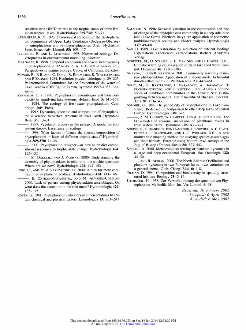
(1) Early disappearance of Group II: The early disappearance of Group II and the appearance of Group III as early as May coincides with the milder winters and springs observed since 1988 (Fig. 8A). Warm average air temperatures are correlated with high values of the North Atlantic Oscil- lation (NAO) index, which also influences water temperatures in several other European lakes (Straile and Adrian 2000; Gerten and Adrian 2001; Scheffer et al. 2001). The NAO is associated with changes in the surface westerlies across the Atlantic into Europe. It characterizes a meridional oscillation in atmospheric mass, with centers of action near the Icelandic low and the Azores high. The NAO is the dominant mode of atmospheric variability in the North Atlantic throughout the year. It is particularly important in winter, when it exerts a strong influence on temperature and precip- itation (Hurrel 1995). As shown in Fig. 8B, warmer winters and springs favor zooplankton growth. Indeed the date of the zooplankton burst appears to be closely correlated with the air temperature index (p < 0.001). The date of the zooplankton burst is also correlated (p < 0.01) with the last day with a phytoplankton assemblage associated with Group II (Fig. 8B). As a consequence, like recent data for Lake Constance

74 76 78 80 82 84 86 88 90 92 94 96 98 Year

120 - R2=0.450, p<0 001 * *

*

*+

90 * Apr - May Jun 90 120 150 180 Herbivorous zooplankton burst

(Day of the year)

74 76 78 80 82 84 86 88 90 92 94 96 98 Year

180 - R2 =0.353. p<0.0 1

150-

120- T *

90 Apr May Jull 90 1 20 1 50 1 80 Herbivorous zooplankton burst

(Day of tlle year)

B _s

X o

._ Q

*- t4_

o o ;F.

a

vX ;N

oo o

Fig. 8. (A) Long-term changes in the differences between the average winter (or spring) air temperatures and the average winter (or spring) temperatures measured at the INRA station from 1974 to 1998. (B) Correlations between the day of year of the herbivorous zooplankton burst versus the temperature precocity index and the day of year of herbivorous zooplankton burst versus the last day for which the sample is characterized by the phytoplankton assemblage associated with Group II.

(Straile 2000), in Lake Geneva, changes in the timing of the clear water phase is also thought to be the consequence of warmer winters and early spring meteorological conditions, which promote the development of zooplankton and enhance their grazing pressure.

(2) Summer colonization of the lake by Group VI: During the recent paradoxical response of algae to a fall in phosphorus, the lake has been colonized in summer by Group VI, associated with R strategists. These observations are consistent with those obtained with the STATIS multitable methods previously applied to the Lake Geneva time series in order to describe the seasonal dynamics of phytoplankton and analyze their stability over the 25 yr (Anneville et al. in press). The environmental parameter that distinguishes between Groups V and VI is principally the depth of the DIP- depleted layer. As a result of the synergism between the decrease in the loading of phosphorus into the lake and the high spring consumption, in the l990s, the DIP-depleted zone appears earlier and extends deeper in the water column (Fig. 6). Later, when the phytoplankton community is characterized by Group VI, the zone of severe DIP depletion extends down to a depth of 30 m in summer. However, despite very low DIP concentrations in the surface water, they are still high in deeper layers, and local water mixing resulting from the breaking of internal waves is likely to sup- ply the metalimnion with phosphorus. In such an environment, species localized in the water layer where there are episodic incursions from the deep, richer layers might be able to gain some advantage. Indeed, as in other lakes in the course of oligotrophication, the actual trend in Lake Geneva is effectively a fast deepening of the phytoplankton (Anne- ville and Leboulanger 2001). And, i3ecause light becomes a critical factor with increasing depth, in such an environment, the most appropriate adaptations are those of a good light- harvesting antenna and of an adaptive ability to increase the




Geneva: A response to the reoligotrophication. Atti Assoc. Ital. Oceanogr. Limnol. 14: 25-35.

, AND J. P. PELLETIER. 2000. Recovery of Lake Geneva from eutrophication: Quantitative response of phytoplankton. Arch. Hydrobiol. 148: 607-624.

, N. ANGELI, V. GINOT, AND J. P. PELLETIER. 2001. Ambi- guite sur ltetat trophique du Leman: vers un indice fonde sur les associations d'especes, p. 153-175. In Cemagref [ed.], Etat de sante des ecosystemes aquatiquese nouveaux indicateurs biologiques. France.

, V. GINOT, J. C. DRUART, AND N. ANGELI. In press. Long- term study (1974-1998) of seasonal changes in the phytoplankton in Lake Geneva: A multi-table approach. J. Plankton Res.

BALVAY, G. 1998. Le zooplancton du Leman compartiment incon- tournable de reseau trophique. Archs Sci. Geneve 51: 45-54.

BERMAN, T., AND B. SHTEINMAN. 1998. Phytoplankton development and turbulent mixing in Lake Kinneret. J. Plankton Res. 20: 709-726.

, Y. Z. YACOBI, AND U. POLLINGHER. 1992. Lake Kinneret phytoplankton: Stability and variability during twenty years (1970-1989). Aquat. Sci. 54: 104-127.

CARPENTER, S. R., AND K. L. CorrlNGHAM. 1997. Resilience and restoration of lakes. Conserv. Ecol., http://www.consecol.org/ vol l/iss l/art2.

COOLEY, W. W., AND P. R. LOHNES. 1971. Multivariate data analysis. Wiley.

CRONBERG, G. 1982. Changes in the phytoplancton of Lake Tru- menn induced by restoration. Hydrobiologia 86: 185-193.

DASI, M. J., M. R. MIRACLE, A. CAMACHO, J. M. SORIA, AND E. VICENTE. 1998. Summer phytoplankton assemblages across trophic gradients in hard-water reservoirs. Hydrobiologia 369/ 370: 27-43.

DUFRENE, M., AND P. LEGENDRE. 1997. Species assemblages and indicator species: The need for a flexible asymmetrical approach. Ecol. Monogr. 67: 345-366.

ELLIorr, J. A., C. S. REYNOLDS, AND T. E. IRISH.2000. The diversity and succession of phytoplankton communities in disturbance-free environments, using the model PROTECH. Arch. Hydrobiol. 149: 241-258.

FERNANDEZ, E., AND A. BODE. 1994. Succession of phytoplankton assemblages in relation to the hydrography in the southern Bay of Biscay: A multivariate approach. Sci. Mar. 58: 191-205.

GAWLER, M., P. BLANC, J. C. DRUART, AND J. PELLETIER. 1986 Dynamique de quelques populations majeures du phytoplancton printanier du lac Leman en relation avec le broutage et les sels nutritifs. Biol. Populations 4: 412-419.

GERTEN, D., AND R. ADRIAN. 2001. Differences in the persistency of the North Atlantic Oscillation signal among lakes. Limnol. Oceanogr. 46: 448-455.

HALL, R. I., AND J. P. SMOL. 1999. Diatoms as indictors of lake eutrophication, p 128-168. In E. F. Stoermer and J. P. Smol [eds], The diatoms: Applications for the environmental and earth sciences. Cambridge Univ. Press.

HARFF, J. E., AND J C. DAVIS. 1990. Regionalization in geology by multivariate classification. Math. Geol. 22: 573-588.

, J. C. DAVIS, AND W. EISERBECK. 1993. Predictions of hy- drocarbons in sedimentary basins. Math. Geol. 25: 925-936.

HORNSTROM, E. 1981. Trophic characterization of lakes by means of qualitative phytoplankton analysis. Limnologica 13: 249- 261.

HURRELL, J. W. 1995. Decadal trends in the North Atlantic Oscil- lation: Regional temperatures and precipitations. Science 269: 676-679.

HUSZAR, V. L. M., L. H. S. SILVA, P. DOMINGOS, M. MARINHO, AND S. MELO. 1998. Phytoplankton species composition is more

cell-specific photosynthetic capacity that is, adaptive traits shared by the R strategists. Furthermore, because these species are large and not well grazed by the zooplankton, they can easily accumulate and lead to the high biomass observed in the last years. Finally, even if the extent to which phytoplankton species become organized and segregated in vertical gradients is very much dependent on density stability and its longevity (Reynolds 1992), one might be tempted to consider that a vertical segregation of species exists. Unfor- tunately, the sampling design does not provide any information about the vertical organization of the dominant algal populations and, therefore, cannot be used to test the effec- tiveness of this hypothesis. Investigations in this direction could be useful in attempting to identify a pattern of this type for the way the phytoplankton community adapts to changes in nutrient loads.

The statistical method applied to the Lake Geneva phytoplankton data set identified six distinct phytoplankton assemblages. The rules underlying phytoplankton assembly are still not clear and remain subject to debate (Rojo et al. 2000). However, assemblages of species and their pattern of succession have been found to be an informative unit for studying the seasonal and long-term dynamic of phytoplankton.

Even though seasonal changes in the phytoplankton community appeared to be greater than interannual ones, the temporal map underlined that this recurrent seasonal dynamic pattern can be upset by events (the NAO and a deepening of the phosphorus-depleted layer) acting at greater spatial and temporal scales than the local meteorological perturba- tions involved in surface forcing.

Furthermore, as pointed out by the trophic template con- cept, changes in species composition seem to be linked to changes in nutrient loading, but it is scarcely a direct consequence of nutrient availability (Reynolds 1998). In Lake Geneva, the vertical distribution of phosphorus and light during summer constitutes a critical component in selecting the species or, more specifically, in selecting a set of species (assemblage) sharing a common ability to benefit from the summer habitat characteristic of the l990s.

Given the observed rapid deepening of the phytoplankton, it is suggested that as long as nutrient concentrations in intermediate water layers remain higher than critical values for phytoplankton growth, we should observe a shift of the pro- ductive base away from the surface and into the functioning of the deep chlorophyll maximum. That is why the sampling depth for the phytoplankton survey was extended down to 20 m (the limit for our integrating sampling device) to take into account the phytoplankton assemblage in deeper parts of the water column.

The paradoxical response of Lake Geneva phytoplankton to a decrease in phosphorus was first seen as disluptive, but the findings of the present study are now seen to be en- couraging with regard to efforts being made both to phosphorus reduction and lake monitoring.

References

ANNEVILLE, O., AND C. LEBOULANGER. 2001. Long-term changes in the vertical distribution of phytoplankton in the deep Alpin




sensitive than OECD criteria to the trophic status of three Bra- zilian tropical lakes. Hydrobiologia 369/370: 59-71.

KUMMERLIN, R. E. 1998. Taxonomical response of the phytoplankton community of Upper Lake Constance (Bodensee-Obersee) to eutrophication and re-oligotrophication. Arch. Hydrobiol. Spec. Issues Adv. Limnol. 53: 109-117.

LEGENDRE, P., AND L. LEGENDRE. 1998. Numerical ecology: De- velopments in environmental modelling. Elsevier.

MARGALEF, R. 1958. Temporal succession and spacial heterogeneity in phytoplankton, p. 323-349. In A. A. Buzzati-Traverso [ed.], Perspectives in marine biology. Unive. of California, Berkeley.

MONOD, R., P. BLANC, C. CORVI, R. REVACLIER, R. WATTENHOFER, AND P. ZAHNER. 1984. Evolution physico-chimique, p. 89-225. In International Committee for the Protection of the water of Lake Geneva (CIPEL), Le Leman, synthese 1957-1982. Lau- sanne.

REYNOLDS, C. S. 1980. Phytoplankton assemblages and their periodicity in stratifying lake systems. Holarct. Ecol. 3: 141-159.

. 1984. The ecology of freshwater phytoplankton. Cam- bridge Univ. Press.

. 1992. Dynamics, selection and composition of phytoplankton in relation to vertical structure in lakes. Arch. Hydrobiol. Beih.35: 13-31.

. 1997. Vegetation process in the pelagic: A model for ecosystem theory. Excellence in ecology.

. 1998. What factors influence the species composition of phytoplankton in lakes of different trophic status? Hydrobiol- ogia 369/370: 11-26.

. 2000. Phytoplankton designer or how to predict compo- sitional responses to trophic-state change. Hydrobiologia 424: 123-132.

, M. DOKULIL, AND J. PADISAK. 2000. Understanding the assembly of phytoplankton in relation to the trophic spectrum: Where are we now? Hydrobiologia 424: 147-152.

ROJO, C., AND M. ALVAREZ-COBELAS. 2000. A plea for more ecology in phytoplankton ecology. Hydrobiologia 424: 141-146.

, E. ORTEGA-MAYAGoITIA, AND M. ALVAREZ-COBELAS. 2000. Lack of pattern among phytoplankton assemblages. Or, what does the exception to the rule mean? Hydrobiologia 424: 133-139.

ROSEN, G. 1981. Phytoplankton indicators and their relations to cer- tain chemical and physical factors. Limnologica 13: 263-290.

SALMASO, N. 1996. Seasonal variation in the composition and rate of change of the phytoplankton community in a deep subalpine lake (Lake Garda, Northern Italy). An application of nonmetric multidimensional scaling and cluster analysis. Hydrobiologia 337: 49-68.

SAS, H. 1989. Lake restoration by reduction of nutrient loading: Expectations, experiences, extrapolations. Richarz, Academia Verlag.

SCHEFFER, M., D. STRAILE, E. H. VAN NES, AND H. HOSPER. 2001. Climatic warming causes regime shifts in lake food webs. Lim- nol . Oceanogr. 46: 1780- 1783.

SMAYDA, T., AND R. REYNOLDS. 2001. Community assembly in marine phytoplankton: Application of a recent model to harmful dinoflagellate bloms. J. Plankton Res. 23: 447-461.

SOLIC, M., N. KRSTULOVIC, I. MARASOVIC, A. BARANOVIC, T. PUCHER-PETKOVIC, AND T. VUCETIC. 1997. Analysis of time series of planktonic communities in the Adriatic Sea: Distin- guishing between natural and man-induced changes. Oceanol. Acta 20: 131-143.

SOMMER, U. 1986. The periodicity of phytoplankton in Lake Con- stance (Bodensee) in comparison to other deep lakes of central Europe. Hydrobiologia 138: 1-7.

, Z. M. GLIWICZ, W. LAMPERT, AND A. DUNCAN. 1986. The PEG-model of seasonal succession of planktonic events in fresh waters. Arch. Hydrobiol. 106: 433-471.

SOUISSI, S., F. IBANEZ, R. BEN HAMADOU, J. BOUCHER, A. C. CATH ELINEAU, F. BLANCHARD, AND J. C. POULARD. 2001. A new multivariate mapping method for studying species assemblages and their habitats: Example using bottom trawl surveys in the Bay of Biscay (France). Sarsia 86: 527-542.

STRAILE, D. 2000. Meteorological forcing of plankton dynamics in a large and deep continental European lake. Oecologia 122: 44-50.

, AND R. ADRIAN. 2000. The North Atlantic Oscillation and plankton dynamics in two European lakes two variations on a general theme. Glob. Chang. Biol. 6: 1-8.

TILMAN, D. 1994. Competition and biodiversity in spatially struc- tured habitats . Ecology 75: 2- 16.

UTERMOHL, H. 1958. Zur Vervollkommung der quantitativen Phy- toplankton-Methodik. Mitt. Int. Ver. Limnol. 9: 38.

Received: 16 January 2002 Accepted: 6 April 2002 Amended: 6 May 2002



temporal mapping of phytoplankton assemblages in lake geneva: annual and interannual changes in...

Documents