Temporal Lensing and its Application in Pulsing

Denial of Service Attacks

Ryan RastiMukul MurthyVern Paxson

Electrical Engineering and Computer SciencesUniversity of California at Berkeley

Technical Report No. UCB/EECS-2014-129

http://www.eecs.berkeley.edu/Pubs/TechRpts/2014/EECS-2014-129.html

May 26, 2014

Copyright © 2014, by the author(s).All rights reserved.

Permission to make digital or hard copies of all or part of this work forpersonal or classroom use is granted without fee provided that copies arenot made or distributed for profit or commercial advantage and that copiesbear this notice and the full citation on the first page. To copy otherwise, torepublish, to post on servers or to redistribute to lists, requires prior specificpermission.

Temporal Lensing and its Application in Pulsing Denial of Service Attacks

Ryan RastiUC Berkeley

Mukul MurthyUC Berkeley

Vern PaxsonUC Berkeley

Abstract

We introduce temporal lensing—a technique that con-centrates a relatively low-bandwidth flood into a short,high-bandwidth pulse. By leveraging existing DNS in-frastructure, we experimentally explore lensing and theproperties of the pulses it creates. We also show howattackers can use lensing to achieve peak bandwidthsmore than an order of magnitude greater than their up-load bandwidth. While formidable by itself in a puls-ing DoS attack, we note how lensing can be compatiblycombined with amplification attacks to potentially allowattackers to produce pulses with peak bandwidths ordersof magnitude larger than their own.

1 Introduction

Denial of service (DoS) first gained significant attentionmore than a decade ago [13], but its essential featureshave largely remained unchanged. That is, DoS attackshave grown larger in scale (most notably with distributeddenial of service, or DDoS), but have often retained themindset of brute-force flooding.

However, there are certain variants on DoS that aremore intelligent. Some exploit abstracted-away featuresof protocols. For example, SYN flooding attempts tomount a state-holding attack in implementations of TCP.In addition to protocols, certain types of DoS attacks alsoexploit existing infrastructure. Reflector attacks [15], forinstance, trick innocent third parties into assisting. Thereflector can serve the dual purpose of hiding the at-tacker’s identity and increasing the efficacy of the attack,usually by reflecting a larger payload to the victim.

The plethora of protocols and deployedinfrastructure—much of it originally designed withlittle regard for security—opens the door to exploitation.We introduce temporal lensing, which (a) exploitsexisting infrastructure (reflectors) in the novel way ofconcentrating a flood in time, and that (b) can be used to

significantly increase the effectiveness of an attack on afeature of a widely deployed protocol (TCP congestioncontrol). We experimentally validate lensing and note itsability to empower an attacker.

2 Related Work

Kuzmanovic and Knightly [8] first describe the conceptof bursty, low average bandwidth pulses as “shrew” at-tacks. The attack aims to send enough packets in a shortduration to cause a TCP RTO (retransmit timeout) inclients and then periodically induce another RTO witheach pulse. They note that such attacks, due to theirlow average bandwidth, are harder to detect than tradi-tional flooding. They show that such an attack is ef-fective at reducing throughput by an order of magnitudeor more. Also, they perform experimentation showingthe drawbacks of two proposed defences. Specifically,RED requires longer measurements to correctly identifyshrew pulses; increased randomization of RTOs involvesa trade-off with throughput in the absence of an attack.

Luo and Chang [12] generalize the idea of shrew at-tacks from attacks on RTO to attacks on TCP congestioncontrol in general. That is, they also consider an attackon TCP’s AIMD (additive increase multiplicative de-crease) mechanism and show that it can also severely de-grade TCP flows. Guirguis et al. [5] further abstract suchlow average bandwidth attacks as a type of RoQ (reduc-tion of quality) attack—that is, pulsing exploits transientsin a system (congestion control for the example of puls-ing), instead of its steady state capacity (victim’s band-width). Their empirical analysis was limited to a systemother than TCP and congestion control (they experimenton bursty web requests effects on system resource utiliza-tion and ability to serve other requests). However, theywere able to show the theoretical and practical potentialof RoQ attacks in general.

While pulsing DoS boasts impressive theoretical andexperimental efficacy, it has seen little use in practice.

We suggest a reason to be as follows: senders are limitedto their uplink bandwidth in a pulse, so simple pulsingcannot intuitively perform better than flooding in termsof damage inflicted. However, the idle time betweenpulses indicates room for improvement. We propose amethod that allows an attacker to send in a flood, butconcentrates this flood into pulses at the victim, allowingthe attacker maximal bandwidth utilization.

Paxson [15] describes the role of reflectors in DoS at-tacks as amplifying the flooded traffic and helping at-tackers evade detection. He also notes the natural useof open DNS resolvers as reflectors. Our attack proto-type takes advantage of this last fact and the abundanceof such resolvers (estimated to be in the tens of millions[16]). However, we take a new angle on reflectors, in-stead using them to concentrate the arrival of packets atthe victim, much like a lens focuses light. This methodis orthogonal to traditional amplification attacks.

The proposed attack requires the ability to calculatelatencies between arbitrary hosts, in our case between areflector and the victim. The first major effort at latencyestimation was IDMaps [4] which calculated distance be-tween any two hosts using a map of network tracers. Af-ter IDMaps, many other systems emerged [14, 3, 18, 17].However, dependence on new protocols or infrastructurelimit these schemes applicability to our proposed attack.

These schemes note certain relevant pitfalls with esti-mating latencies. Namely, Ledlie et al. [9] discuss fac-tors which cause differences between expected and ac-tual latency between hosts. One unavoidable factor isthat latencies can be skewed by certain anomalous datasuch as timeouts, which Ledlie et al. [10] remedy by us-ing medians instead of means and employing various fil-ters. We borrow some of these methods (specifically giv-ing less weight to outliers in favor of medians and outlier-independent measures) when building our estimates oflatencies.

Another latency estimation system, Gummadi et al.’sKing [6] offers the impressive advantage that it does notneed additional architecture or cooperation beyond whatis currently found in DNS. King works by finding DNSservers close to the end hosts, and estimating distancesusing recursive DNS queries. King is particularly wellsuited to our task because: (a) it requires no additionalarchitecture or explicit agreement beyond standard DNSqueries, (b) it is most accurate if either (or both) hosts areDNS servers, and (c) recursive protocols, such as DNS,naturally lend themselves to use in reflection. We also in-troduce an addition to King—by taking its cache poison-ing trick a step further—allowing for a direct round-triptime computation between an open DNS resolver and anarbitrary host in Section 7.1.

(a) At t = 0, attacker sends one packet towards re-solver 2

(b) At t = 1, the first packet is halfway along its pathto the victim and the attacker sends another packetto resolver 1

(c) At t = 2, both packets arrive at the victim

Figure 1: Attack illustration. Paths through reflectors1 and 2 have attack path latencies of 1 and 2 secondsrespectively. The attacker sends at a rate of 1 pps, buthe concentrates his flow such that two packets arrive inone second at the victim. For a brief moment, he haseffectively concentrated his bandwidth two-fold.

3 The Attack

3.1 Motivation and Attack DescriptionA normal pulsing attack has one major place for im-provement: a majority of the attacker’s bandwidth is un-used in between pulses. Therein lies the question of howto send packets during these idle times but have thesepackets still arrive at the victim within a pulse.

We draw an analogy to the military strategy “Time onTarget” [7] to synchronize artillery fire. Using synchro-nized clocks and estimates of projectile flight times, acoordinated military can fire from different locations buthave all their fire hit the target at the same time. In amore modern version of this idea, “Multiple Rounds Si-multaneous Impact”, a single artillery can make multiplerounds rendezvous at the target by varying the angle offire, charge, and thus the flight time. By varying pro-

2

jectile paths, an artillery can make more shots arrive atthe victim in one period of time than it can send in thatperiod. We leverage the wide range of paths and laten-cies on the Internet to accomplish a similar feat. If anattacker can schedule sending in such a way that the at-tacker first sends packets that will take longer to arriveand then sends those that will take shorter to arrive, theycan rendezvous within a small window of time.

However, if the attacker sends directly to the victim,the latency is constant. Every packet will take about thesame amount of time to reach the victim since they travelalong the same path.

Reflectors introduce the ability to have variable attackpath latencies: the time from attacker through reflectorto victim. Each reflector used potentially introduces anew path for attack traffic and thus a different attack pathlatency. A simple example is illustrated in Figure 1.

In the remainder of this paper, we will call this tech-nique temporal lensing or simply lensing, as reflectorscan temporally concentrate packets, much like a lens fo-cuses light. Also, when describing how the attack works,we prefer the term concentration to amplification, as theformer is more fitting and the latter is already used todescribe an orthogonal attack.

3.2 StrategyThe actual attack can be decomposed into three mainparts, which we develop in the next three sections of thepaper:

• determining attack path latencies through resolversto the victim (Section 4)

• building a sending schedule to create maximal lens-ing from these latencies (Section 5)

• conducting the attack (Section 6)

After experimentally validating lensing, we turn our at-tention to extensions to our basic attack (Section 7) andfinally to defenses (Section 8).

4 Obtaining latencies on the Internet

To actually carry out the attack using some set of reflec-tors, we first need to know, for each reflector, the attackpath latency. Estimating attacker to reflector and attackerto victim latencies are trivial—any sort of ping will suf-fice. We still need a way to measure latency from thereflector to victim.

Measuring latencies between two Internet end hosts,however, is a well studied problem [4, 14, 3, 18, 17]. Wechose a particular method, King [6], that is particularly

Figure 2: The operation of King (reprinted with approvalfrom [6]), with the relevant actors for lensing added inred

well suited to our task. King operates by issuing recur-sive DNS queries between two DNS servers located closeto the end servers in question. In Figure 2 we use a fig-ure from King and overlay it with labels of the attacker,victim, and reflector, which are features of our attack.The figure shows how, with a single recursive query, anattacker can get an estimate for the attack path RTT, bytaking the difference in time between when the attackersends the query to when the attacker receives a response.

King must deal with two conflicting caching issues.First, it “primes” the resolver so that it caches the factthat the victim is authoritative for its domain. This pre-vents the resolver from iterating through the DNS hi-erarchy for a query. Second, the attacker must issuequeries for different subdomains of the domain the vic-tim (foo.bar in the example), lest the attacker hit theresolver’s cache and short-circuit the query. King (andour attacker) bypasses this last issue by sending queriesfor random subdomains, each of which requires the en-tire chain of packets 1-4 in the figure to be sent.

So, for our attack, if we limit our reflectors to recursiveDNS resolvers (which by their recursive nature can per-form such reflection naturally), such estimates are mademore accurate. If we further limit the victim to a DNSserver1 as well, then King accurately measures the attackpath RTT, which can be halved to obtain the attack pathlatency. One may intuit that halving the RTT may givea one-way latency, but this by no means needs to be thecase. Our positive experimental results on lensing andpulsing in Section 6, however, experimentally validate

1The reader may correctly note that pulsing DoS attacks (whichattack TCP congestion control) will probably have little impact on aUDP based service with short quasi-flows such as DNS. We defer adiscussion of estimating attack path latencies to TCP-based hosts toSection 7.1

3

Figure 3: Two good resolvers (Google and Eindhoven University of Technology) with minimal path latency variation(roughly flat lines), an obviously bad resolver with high path latency variation (where 1000ms is a timeout), and aresolver that appears good over small samples of time but is actually bad for our attack, respectively. We took samples2 minutes apart.

this heuristic.In short, King provides a suitable method for estimat-

ing the attack path latency.

4.1 Open DNS Resolvers

We take a short detour to discuss relevant practical as-pects of DNS.

[16] has put recent estimates of the number of openDNS resolvers in tens of millions, with many running on(often outdated) commodity hardware. Further it notesthat many of such resolvers are ephemeral and last on agiven IP on the order of days to weeks.

[16] also notes that many resolvers do not iterate theDNS hierarchy themselves, but instead forward the workoff to auxiliary resolvers. TurboKing [11], an extensionof King, explicitly acknowledges this possibility to im-prove its accuracy. However, since the traffic for our at-tack will follow the same path as that for determininglatencies, such DNS nuances should not affect the attackpath latency calculations.

4.2 Attack Path Latency Variation

4.2.1 Short-term Variation

One point of concern is how accurate attack path latencymeasurements are over a short period of time. In partic-ular, it may take a few minutes to just measure latenciesto all of the resolvers (as is the case for our prototype).We want to explore how attack path latencies vary overthis period of time. Depending on how much they do, itmay render just minutes-old estimates invalid.

To this end, we took a sample of 44 resolvers from apublic list of about 3000 [1] and measured the path la-

tency through each one once every two minutes.2 Fig-ure 3 shows selected examples of what the path latencieslooked like over time in the cases of (from the attacker’spoint of view): good latency variation, bad variation, anddeceptively good variation.

After taking a few samples over a few seconds, itwould be obvious that the resolvers in the first graph aregood3 and the resolver in the second graph are not. How-ever, the resolver in the third graph may also be consid-ered good because it had few timeouts and a fairly consis-tent latency over a short period of time. But over longerperiods of time, it looks as if there are routing changesthat abruptly change the attack path latency; this couldcause packets sent to this resolver to miss the pulsingwindow.

We found that the interquartile range (IQR, which isdefined as the difference between the 75th and 25th per-centiles) was an effective feature for identifying thesemisleading resolvers. Fortunately for an attacker, thesemisleading resolvers are also rare; while the one in thatthird graph had an IQR of 122 ms, Figure 4 shows thatalmost half our resolvers had an IQR of less than 12 ms.

So for some resolvers, the attacker must either per-form latency measurements immediately before the at-tack or have a longer period of statistics to show that theresolver is not a good one and not use it. However, asFigure 4 shows, these types of resolvers are uncommon.So even if an attacker does not account for the cases ofmisleading resolvers and just assumes every resolver thatappears good over a short period of time is indeed good,performance will not significantly suffer.

2We take appropriate measures (previously discussed) to make sureDNS caching does not invalidate our results.

3The spikes represent timeouts, which disproportionately distort thegraph. For resolvers where they occur infrequently, we believe them tobe the result of low (but non-zero) packet loss rates.

4

Figure 4: Cumulative Distribution Function of IQRranges of path latencies for each resolver, with samplestaken every 2 minutes over 24 hours.

4.2.2 Long-term Variation and Caching

Since we have just discussed some challenges gainingaccurate measurements of path latencies through dif-ferent resolvers and declaring resolvers good, it makessense to consider caching these results to save time andbandwidth computing them again later on. Note that be-fore we were worried about how steady a resolver is overa period of minutes; now we are concerned about thevalidity of that measurement over the course of days orweeks.

To examine how the latencies change over longer pe-riods of time, we took our same sample of resolvers andsent 50 packets (after taking care to warm-up NS recordcaching and bypass A record caching) through each re-solver every 4 hours for about 10 days. For each resolverand each set of measurements, we took the median of the50 latencies. For each resolver, we computed the stan-dard deviation of these medians for each sample time(there were a total of 59 of these medians, assuming allmeasurements were successful for that resolver). Sincewe are interested in comparing variation, we divided thestandard deviations by the means; these terms are calledcoefficients of variation and are normalized standard de-viations. The distribution of these coefficients of varia-tion are shown in Figure 5.

Since the data shows that some resolvers have very lit-tle variance over time, we believe that many resolvers’measurements can be cached. Resolvers with coeffi-cients of variation below a certain threshold (we believe0.02 is reasonable) have consistent path latencies, andtheir latency times can be cached. If we were to runthe same statistics on a much larger group of resolvers- which would take excessive time and bandwidth - we

Figure 5: Box plot of the coefficients of variance of eachresolver’s set of medians. A low CV suggests that a re-solver’s path latency to the victim did not change muchover the course of our 10-day period.

would be able to identify a large set of these resolversand save a shortlist of high-quality resolvers to speed upfuture attacks.

We also note that we did not find many resolvers withhigh attack path latencies. Having resolvers with highpath latencies (with low variation) would enable us to in-crease our theoretical bandwidth gain because we wouldhave a longer period of time to send packets over (andsubsequently concentrate). However, we found that mosthigh latency paths exhibited high jitter and inconsistency.As Figure 6 shows, none of the resolvers in our samplewith more than 450 ms latency had a coefficient of vari-ance below 0.02, and resolvers over 600 ms latency hadabout 0.1 coefficient of variance or greater. This makessense because higher latency paths generally have morehops, which means more room for inconsistencies.

4.3 Amplification Attacks

Since we are using DNS resolvers as reflectors, it mayoccur to the reader that lensing can be combined withamplification. To study pulsing in isolation, however, wewill concentrate solely on lensing and defer a discussionto how amplification might be added to the attack and itsconsequences to Section 7.2.

Lastly, we emphasize that DNS is simply our chosenvector for the attack because of: its simplicity in deter-mining latencies, the availability of recursive DNS re-solvers, and the fact that recursion allows reflection with-out IP spoofing. However, essentially any type of reflec-tion is compatible with lensing.

5

Figure 6: Plot of the average latency of each resolveragainst that resolver’s coefficient of variance, as com-puted earlier. Three resolvers had CVs greater than 0.4and are not shown.

5 Building an Optimal Schedule

Now that we have obtained path latency estimates forresolvers, we must compute a sending schedule. Thisschedule divides up the sending window into a set of timeslots T and states which resolver an attacker should sendto for each slot. The number of slots available for theattacker to send is a function of the attacker’s maximumbandwidth and the range of path latencies measured fordifferent resolvers.

We have some set of reflectors R and set of time slotsto send T . Define the pulse window or simply window tobe the duration of the pulse as seen at the victim. In try-ing to create the largest pulse, our goal is maximize theexpected number of packets that land in a predeterminedwindow. We use a greedy algorithm to compute the op-timal schedule given an initial set of reflectors and esti-mates of their corresponding attack path latencies. Ac-cording to our algorithm, at each time slot t, we simplychoose the reflector which provides the highest estimatedprobability of landing within the window. This greedy al-gorithm is indeed optimal. We defer a proof to Section12.

However, the problem statement and proof do not ac-count for distortions in the attack path latencies due to theattack itself—such as those caused by effects of strain-ing resolvers and congestion caused by the attack. Sincethe attack is distributed over geographically diverse re-solvers, any congestion should decrease exponentiallywith the number of hops from the victim. So, it is notclear if congestion would actually be detrimental froman attacker’s point of view. Further, we find little evi-dence of congestion that would actually inhibit an attack

in our experimentation.

6 Attack Experimentation

Armed with the ability to estimate attack path latenciesand to build an optimal schedule from them, we are fi-nally ready to experiment with lensing.

6.1 Methodology

We simulate attacks on machines under our control. Weuse an Windows Azure VM instance on the West Coastas our attacker. We use another Azure VM instance andan Amazon Web Services VM instance, both on the EastCoast, as our victims. We use a publicly available list ofjust over 3,000 resolvers [1] as our reflectors.

We register a domain name4 that allows us to have anauthoritative DNS server. We make the AWS victim in-stance authoritative for our domain and the Azure victiminstance authoritative for a subdomain of the original.This allows us to send recursive DNS queries throughany open recursive DNS server to either of our victims.

Before an attack, the attack machine quickly scans theresolver list. It issues recursive queries to the resolvers(just as in the attack) to obtain latency measurements.5

For each resolver, it constructs a histogram for the dis-tribution of each attack path latency. Then, it essentiallyperforms the optimization algorithm in Section 5 withthe histograms serving to compute probabilities. Duringthe attack, we just send to the resolvers according to theschedule.

6.2 Features Measured

6.2.1 Dimensions

We measure pulsing on a few dimensions—specificallyhow our attack metrics vary as a function of:

• attacker bandwidth (to simulate attacker’s with dif-ferent resources, we throttle our sending appropri-ately)

• maximum bandwidth to each reflector (to see howthis affects this attack, and to avoid overburdeningor getting throttled by a resolver)

• pulse window size (the duration during which weare trying to have packets arrive at the victim)

4pulsing.uni.me5We chose to take ten samples from each resolver, which turned out

well for our attack

6

In addition, the attacker might have separate reasons ownfor throttling bandwidth to any given reflector (for ex-ample to avoid arousing suspicion). Also, since the re-sources of the reflectors we use are unknown, we err onthe side of caution when sending to them. To any givenone, we send at a maximum bandwidth of 500 pps over acourse of 20-100 ms (which translates to a maximum of5 KB).

We do not explicitly explore the number of reflectorsused as a dimension, because the number of reflectorsheavily depends on the existing dimensions of attackerbandwidth and maximum bandwidth to each reflector.

6.2.2 Metrics

In Section 5 we defined an optimal schedule as onethat has the greatest expected amount of packets fallingwithin the pulse window. This is intuitively a natural pa-rameter to maximize. However, if we solely use absolutenumber of packets as our metric of efficacy, it will be ar-tificially inflated just by increasing the uplink bandwidthof the attacker or increasing the target window size. So,we choose some additional bandwidth-agnostic metrics:

• bandwidth gain: bandwidth in the pulse window at the victimattacker’s maximum sending bandwidth

• concentration efficiency: # packets landing in window# total packets sent

The first metric is the most important from the short-term point of view of the attacker. It gives the attacker asense of how much extra bandwidth can be produced.

The second metric, however, provides a good basisfor determining how the attack scales with the attacker’sbandwidth. Because the size of the reflector pool is con-stant, as we increase sending (i.e., attacker) bandwidth,there will be more time slots when there will be no avail-able resolver to send to (because we throttle bandwidthto any given reflector). In this case, the bandwidth gainwill artificially decrease. To see this, imagine we send amaximum of one packet to each of 100 reflectors—thenwe can at most send 100 packets to the victim, regardlessof our uplink bandwidth. However, all things equal, theconcentration efficiency will remain constant.

These two metrics must be used in conjunction witheach other, as it is easy to inflate one metric at the ex-pense of the other. A large pulse window size would leadto concentration efficiency of 1 (ignoring packet drops)but no bandwidth gain. An ultra-small target windowcould result in an extremely high bandwidth gain (if onepacket lands in it) but a very low concentration efficiency.

Lastly, we measure bandwidth in terms of packets persecond. The packets we send and that are reflected aresmall (around 100 bytes), which may make the num-bers look artificially high. For a sense of scale, 10K ppsroughly translates to 8 Mbps.

6.3 Results

Figure 7 shows the results of a pulse simulating attackerswith different bandwidths at a fairly thin pulse windowof 20 ms. The simulation artificially caps our outgoingbandwidth by appropriately adjusting the minimum timebetween which any two packets can be sent. The band-width gain can essentially be calculated by dividing theheight of the pulse bucket by that of the tallest bucket forthe attacker’s sending. For the low-bandwidth case, wesee a gain of slightly over 14 times for low bandwidth,10 times for the moderate bandwidth, and 5 times for thehigh bandwidth. The efficiency can be calculated by di-viding the area of the pulse bucket by that of all the buck-ets on the left (sending) graph. The efficiency is around50% for the low and medium cases and just under 40%for the high bandwidth case.

The colors on Figure 7a map onto the reflectors used—we can see that a number of reflectors contribute to thepulse and some do not at all (because their latency mea-surements were off).

We see what look like multiple pulses on Figures 7band 7c. The packet traces reveal that these secondaryspikes are retransmits by the resolvers. The victim (anauthoritative DNS server) was not able to keep up withthe rate of queries and failed to respond to many of them.The resolvers then timeout and retransmit; since manyof them share a common retransmit timeout, their re-transmits rendezvous at time = (original pulse time) +(retransmit timeout). We were able to determine, then,two common retransmit timeouts of 800 ms and 2 s. Wediscuss some ways an attacker may be able to leverageretransmits in section 7.4.2. Another feature of retrans-mits is that the total number of packets received by thevictim often exceeds the total number sent by the attackerby about a factor of two.6

Figure 8 shows how the lensing metrics vary withpulse window duration (the dimensions attacker band-width 10K pps, max bandwidth to reflector of 500 pps arefixed). Bandwidth gain (and absolute pulse bandwidth)are expected to fall as window size increases because weare essentially spreading the pulse out. Efficiency sees aslight increase, but seems to level off at larger windowsizes. We hypothesize that there are a number (about40%) of reflectors that show an extremely high attackpath latency variation but are nonetheless chosen as re-flectors.

Figure 9 shows lensing properties as a function ofmaximum bandwidth to any reflector (dimensions at-tacker bandwidth 10K pps, window size 20 ms are fixed).The variation in the metrics of bandwidth gain and pulsebandwidth are not too illuminating, since they vary only

6But our metrics are carefully chosen so that retransmits do not af-fect them.

7

(a) Pulse from Low Bandwidth (500 pps) sending, 75 reflectors sent to

(b) Pulse from Medium Bandwidth (10,000 pps) sending, 816 reflectors sent to

(c) Pulse from High Bandwidth (20,000 pps) sending, 1201 reflectors sent to

Figure 7: Selected Pulses performed on the AWS Instance (using dimensions of max bandwidth to reflector 500 pps,window size 20 ms). The bucket size is set equal to the pulse window size (20 ms).

8

(a) Bandwidth Gain

(b) Concentration Efficiency

(c) Pulse Bandwidth

Figure 8: Lensing Metrics as a Function of the DesiredPulse Window Size (with the AWS instance as victim—fixed dimensions: attacker bandwidth 10K pps, maxbandwidth to reflector of 500 pps)

(a) Bandwidth Gain

(b) Concentration Efficiency

(c) Pulse Bandwidth

Figure 9: Lensing Metrics as a Function of ThrottledBandwidth to Each Reflector (with the AWS instance asvictim—fixed dimensions: attacker bandwidth 10K pps,window size 20 ms)

9

(a) Bandwidth Gain

(b) Concentration Efficiency

(c) Pulse Bandwidth

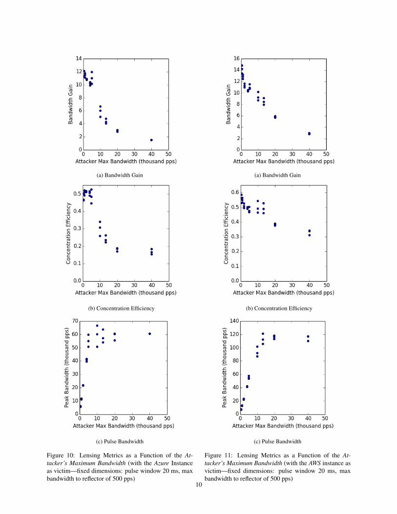
Figure 10: Lensing Metrics as a Function of the At-tacker’s Maximum Bandwidth (with the Azure Instanceas victim—fixed dimensions: pulse window 20 ms, maxbandwidth to reflector of 500 pps)

(a) Bandwidth Gain

(b) Concentration Efficiency

(c) Pulse Bandwidth

Figure 11: Lensing Metrics as a Function of the At-tacker’s Maximum Bandwidth (with the AWS instance asvictim—fixed dimensions: pulse window 20 ms, maxbandwidth to reflector of 500 pps)

10

because of high throttling of bandwidth to a constantsize pool of reflectors (discussed in more detail section6.2.2). The illuminating metric is that of concentrationefficiency. We see little variation, except for at veryhigh throttling (effectively sending a maximum of 1 or2 packets to reflector), where there is high efficiency.With these high efficiencies, however, comes no band-width gain, meaning that there was no pulse created dueto excessive throttling. Due to lack of variation in effi-ciency, we conclude that there is little to be gained bylimiting the bandwidth to each reflector. That said, wedid not investigate sending over 500 pps to a reflector foraforementioned reasons, and we are hesitant to extrapo-late these results.

Figure 10 shows how the attack scales as a functionof the attacker’s bandwidth (we fix the pulse window to20 ms and a maximum peak bandwidth of 500 pps toeach reflector). The relatively constant efficiency at thebeginning indicates that the attack scales well; the drop-ping bandwidth gain can be explained by the fact thatwe throttle bandwidth to each reflector while keeping thepool of available reflectors constant (as discussed in Sec-tion 6.2.2). However, we see all metrics perform poorlyat higher bandwidths. Figure 10c offers a potential clue:it should scale linearly with the attacker’s bandwidth, butinstead we see it level off at about 50-60 thousand pack-ets per second—meaning that the largest pulse we cancreate of duration 20 ms has bandwidth of 50-60K pps.

Now, there are two main explanations for this apparentpulse degradation at scale: either that (a) it is a feature ofthe attack scaling poorly, or (b) it is due to the attackworking—increased jitter and queuing that would causepulse flattening or packet loss would actually be expectedin a successful attack.7

To determine the cause of the poor scaling of theAzure instance, we flooded it at a rate of 100K pps fora short duration. After three trials, we found the maxi-mum download bandwidth for small DNS packets to bebetween 56.8K and 62.4K pps; thus, we conclude that thescaling issues are a sign of the attack’s efficacy—namelythat it saturated Azure’s bottleneck resource in receivingthese packets.

To further corroborate this attribution, we also triedthe same tests on the AWS instance which we found cantake more packets per second (Figure 11). Here the at-tack only starts to scale poorly at much higher peak band-widths of about 110-120K pps—further evidence that theattack was not exhibiting poor scaling on the Azure in-stance. Unfortunately we were not able to generate morethan a 100K pps8 flood, so we were not able to directly

7Of course, we are assuming that measurement error is 0. To thisend, we note that the packet capture tool we used, tcpdump reportedno packet drops.

8The reader may wonder how we came up with the 110-120K pps

determine with certainty what causes the poor scaling at120K pps.

However, the difference in behavior between theAzure and AWS instances with regards to unaccountedfor packets provides a hint in attributing the 120K ppsleveling. We define unaccounted for packets as those thatare sent by the attacker but whose reflection is never re-ceived at the victim. There are some subtleties here. Dueto retransmits, almost all of the sent packets arrive even-tually. So, we redefine “unaccounted” packets as thosethat do not arrive within 200 ms of the pulse window(which for the figures is only 20 ms) to avoid the poten-tial problems with retransmitted packets.

Now, in Azure, it seems as if a router buffers the pack-ets beyond the VM’s quota when the burst is too high, ascan be seen by the pulse spreading in Figure 12, but theAWS instance does not (compare to Figures 7b and 7c).Instead, the reflected packets never appear at the AWSend. Figures 13 and 14 quantify this difference. Withthe Azure instance as victim, we see a relatively constantproportion amount of unaccounted packets to those sent;thus, we see that the attack delivers most of the packets—even at high attacker bandwidths. However, at thesehigher bandwidths, the AWS victim receives much fewerof these packets, as shown in Figure 14. It appears asthough AWS (most likely not the VM, but AWS routers)responds to an excessive download by dropping packets,instead of queuing them as does Azure. So, this discrep-ancy between Azure and AWS indicates that the attackis indeed effective (from the Azure results, we know al-most all of the reflected packets arrive at the East Coast,but they are most likely just dropped by AWS routers be-fore getting to our VM) and that the leveling-off at 120Kpps is due to a limit on the end of AWS.

In short, the attack displays impressive numbers andscales well. As the peak pulse bandwidth nears the vic-tim’s maximum capacity, however, the attacker sees di-minishing returns.

7 Extending the Attack

7.1 Attacks on Arbitrary End-hostsWe previously limited our attack to one on DNS name-servers. Since DNS typically operates over UDP withextremely short flows (if they can even be called such),the efficacy of a pulsing attack (which attacks TCP con-gestion control) is low. Clearly, an attacker would wishto target a more rewarding victim. However, to attackan arbitrary end-host (and not just a authoritative DNS

poor scaling range while being unable to generate more than 100K pps.The answer is that the attacker’s sending bandwidth could not exceed100K pps, but at the receiving end of the attack, the packets concen-trated into a higher 120K pps pulse

11

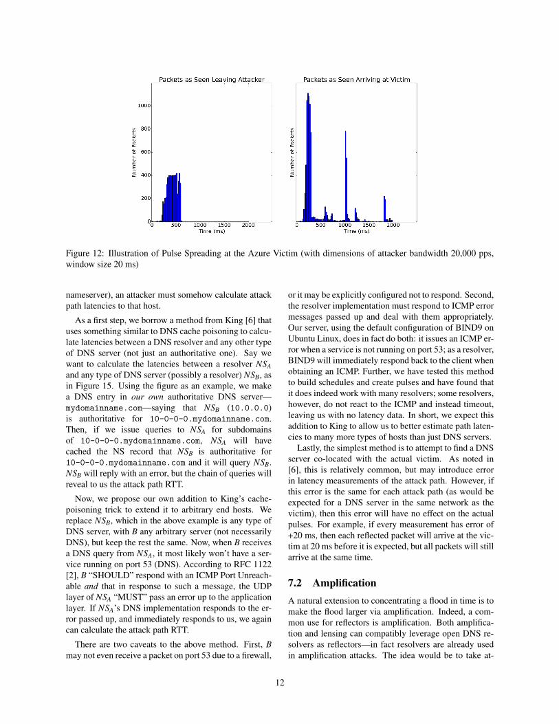
Figure 12: Illustration of Pulse Spreading at the Azure Victim (with dimensions of attacker bandwidth 20,000 pps,window size 20 ms)

nameserver), an attacker must somehow calculate attackpath latencies to that host.

As a first step, we borrow a method from King [6] thatuses something similar to DNS cache poisoning to calcu-late latencies between a DNS resolver and any other typeof DNS server (not just an authoritative one). Say wewant to calculate the latencies between a resolver NSAand any type of DNS server (possibly a resolver) NSB, asin Figure 15. Using the figure as an example, we makea DNS entry in our own authoritative DNS server—mydomainname.com—saying that NSB (10.0.0.0)is authoritative for 10-0-0-0.mydomainname.com.Then, if we issue queries to NSA for subdomainsof 10-0-0-0.mydomainname.com, NSA will havecached the NS record that NSB is authoritative for10-0-0-0.mydomainname.com and it will query NSB.NSB will reply with an error, but the chain of queries willreveal to us the attack path RTT.

Now, we propose our own addition to King’s cache-poisoning trick to extend it to arbitrary end hosts. Wereplace NSB, which in the above example is any type ofDNS server, with B any arbitrary server (not necessarilyDNS), but keep the rest the same. Now, when B receivesa DNS query from NSA, it most likely won’t have a ser-vice running on port 53 (DNS). According to RFC 1122[2], B “SHOULD” respond with an ICMP Port Unreach-able and that in response to such a message, the UDPlayer of NSA “MUST” pass an error up to the applicationlayer. If NSA’s DNS implementation responds to the er-ror passed up, and immediately responds to us, we againcan calculate the attack path RTT.

There are two caveats to the above method. First, Bmay not even receive a packet on port 53 due to a firewall,

or it may be explicitly configured not to respond. Second,the resolver implementation must respond to ICMP errormessages passed up and deal with them appropriately.Our server, using the default configuration of BIND9 onUbuntu Linux, does in fact do both: it issues an ICMP er-ror when a service is not running on port 53; as a resolver,BIND9 will immediately respond back to the client whenobtaining an ICMP. Further, we have tested this methodto build schedules and create pulses and have found thatit does indeed work with many resolvers; some resolvers,however, do not react to the ICMP and instead timeout,leaving us with no latency data. In short, we expect thisaddition to King to allow us to better estimate path laten-cies to many more types of hosts than just DNS servers.

Lastly, the simplest method is to attempt to find a DNSserver co-located with the actual victim. As noted in[6], this is relatively common, but may introduce errorin latency measurements of the attack path. However, ifthis error is the same for each attack path (as would beexpected for a DNS server in the same network as thevictim), then this error will have no effect on the actualpulses. For example, if every measurement has error of+20 ms, then each reflected packet will arrive at the vic-tim at 20 ms before it is expected, but all packets will stillarrive at the same time.

7.2 AmplificationA natural extension to concentrating a flood in time is tomake the flood larger via amplification. Indeed, a com-mon use for reflectors is amplification. Both amplifica-tion and lensing can compatibly leverage open DNS re-solvers as reflectors—in fact resolvers are already usedin amplification attacks. The idea would be to take at-

12

(a) Absolute Number of Unaccounted Packets

(b) Proportion of Unaccounted Packets

Figure 13: Unaccounted Packets as a Function of At-tacker’s Maximum Bandwidth (with the Azure instanceas victim)

tack path latency measurements through reflectors usingthe methods we borrow from King and during the actualattack use these same reflectors for amplification.

Note that the form of lensing we have explored doesnot use source address spoofing to enable reflection; in-stead it relies on recursive queries. However, DNS-basedamplification does require spoofing. While spoofingshould work just fine with lensing, we decided against itfor our experimentation for simplicity and also to avoidconfusing analysts potentially investigating our traffic.

In such a scenario, the attacker would gain the bestof both worlds. For example, an amplification factor of15 and lensing bandwidth gain of 10 could, at its worst,allow attackers to create pulses at 150 times their uplink

(a) Absolute Number of Unaccounted Packets

(b) Proportion of Unaccounted Packets

Figure 14: Unaccounted Packets as a Function of At-tacker’s Maximum Bandwidth (with the AWS instance asvictim)

bandwidths!Forwarders (discussed in Section 4.1) introduce a po-

tential caveat to estimating attack path latencies in am-plification attacks. If the resolver the attacker contacts isindeed a forwarder, then during the attack path latencymeasurements, there are two intermediary hops betweenattacker and victim instead of just one. This was nota problem for our attack, since attack traffic followedthe same path as latency measurements (attacker⇒ for-warder⇒ resolver⇒ victim). However, in an amplifica-tion attack, it would be expected that the attacker wouldplace a large query response in a cache. If it is cachedin the forwarder, then the path of the actual attack trafficwill be one hop shorter (attacker⇒ forwarder⇒ victim).

13

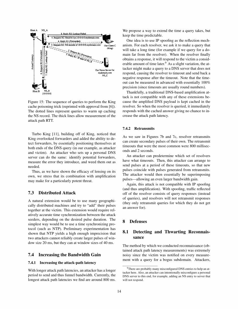
Figure 15: The sequence of queries to perform the Kingcache poisoning trick (reprinted with approval from [6]).The dotted lines represent queries to warm up cachingthe NS record. The thick lines allow measurement of theattack path RTT.

Turbo King [11], building off of King, noticed thatKing overlooked forwarders and added the ability to de-tect forwarders, by essentially positioning themselves atboth ends of the DNS query (in our example, as attackerand victim). An attacker who sets up a personal DNSserver can do the same: identify potential forwarders,measure the error they introduce, and weed them out asneeded.

Thus, as we have shown the efficacy of lensing on itsown, we stress that its combination with amplificationmay make for a particularly potent threat.

7.3 Distributed Attack

A natural extension would be to use many geographi-cally distributed machines and try to “add” their pulsestogether at the victim. This extension would require rel-atively accurate time synchronization between the attackseeders, depending on the desired pulse duration. Thesimplest way would be to use a time synchronizing pro-tocol (such as NTP). Preliminary experimentation hasshown that NTP yields a high enough imprecision thattwo attackers cannot reliably create larger pulses of win-dow size 20 ms, but they can at window sizes of 40 ms.

7.4 Increasing the Bandwidth Gain

7.4.1 Increasing the attack-path latency

With longer attack path latencies, an attacker has a longerperiod to send and thus funnel bandwidth. Currently, thelongest attack path latencies we find are around 800 ms.

We propose a way to extend the time a query takes, butkeep the time predictable.

One idea is to use IP spoofing as the reflection mech-anism. For each resolver, we ask it to make a query thatwill take a long time (for example if we query for a do-main far from the resolver). When the resolver finallyobtains a response, it will respond to the victim a consid-erable amount of time later.9 As a slight variation, the at-tacker might make a query to a DNS server that does notrespond, causing the resolver to timeout and send back anegative response after the timeout. Note that the time-out can be measured in advanced with essentially 100%precision (since timeouts are usually round numbers).

Thankfully, a traditional DNS-based amplification at-tack is not compatible with any of these extensions be-cause the amplified DNS payload is kept cached in theresolver. So when the resolver is queried, it immediatelyresponds with the cached answer giving no chance to in-crease the attack path latency.

7.4.2 Retransmits

As we saw in Figures 7b and 7c, resolver retransmitscan create secondary pulses of their own. The retransmittimeouts that were the most common were 800 millisec-onds and 2 seconds.

An attacker can predetermine which set of resolvershave what timeouts. Then, this attacker can arrange tosend pulses at a period of these timeouts, so that newpulses coincide with pulses generated from retransmits.The attacker would then essentially be superimposingpulses—allowing an even larger bandwidth gain.

Again, this attack is not compatible with IP spoofing(and thus amplification). With spoofing, traffic reflectedoff of the resolver consists of query responses (insteadof queries), and resolvers will not retransmit responses(they only retransmit queries for which they do not getan answer for).

8 Defenses

8.1 Detecting and Thwarting Reconnais-sance

The method by which we conducted reconnaissance (ob-tained attack path latency measurements) was extremelynoisy since the victim was notified on every measure-ment with a query for a bogus subdomain. Attackers,

9There are probably many misconfigured DNS entries to help an at-tacker here. Also, an attacker can intentionally misconfigure a personalDNS server to this end, for example, adding an NS entry to server thatwill not respond.

14

however may be able to hide their presence by makingqueries for legitimate subdomains.10

Perhaps the victim can thwart reconnaissance by poi-soning attack path RTT measurements. The victim can,for example, introduce artificial jitter. The most obvi-ous approach, just adding a random delay to each requestwill only slow down an attacker—by taking more mea-surements an attacker can cut through the noise and de-termine actual latencies. Instead, the victim might intro-duce an amount of jitter as a function of the resolver’saddress. Ideally this function would be keyed and cryp-tographically secure in the sense that knowing one jitterwould not reveal information of another.

However, none of this analysis considers that an at-tacker may be able to take measurements to a nearbyserver not under the victim’s control. In this case, thevictim will not be able to detect reconnaissance at all.Without detection, the victim has little chance of thwart-ing reconnaissance.

8.2 Detecting and Preventing Attacks[8] suggests two methods to mitigate bursty attacks tar-geting TCP’s RTO mechanism: RED and RTO random-ization. The former method proves largely ineffective,while the latter involves a trade-off with throughput inthe absence of an attack. [12] discusses a method to sim-ply detect the presence of a pulsing DoS attack basedon the observation in high variability traffic to the vic-tim (characteristic of a pulse) and subsequent decline inACK traffic back. However, our focus here is on how onemight defend against the lensing side of the attack.

Again, our defense revolves around introducing arbi-trary jitter. A possible mechanism would be for routers tosomehow add jitter during an attack. While it is unclearhow they might coordinate such a mechanism withoutintroducing collateral damage, we explore how it mightplay out in Figure 16. We add a uniform, random amountof jitter after a sending schedule is produced, which is es-sentially the same effect routers adding jitter would have.The graph indicates that cutting a relatively small win-dow pulse of 20 ms in half would require adding jitter of60 ms11 to the attack path.

In short, smart attackers can completely hide their re-connaissance from the victim. Mitigating an actual lens-ing attack would require somehow changing attack pathlatencies during an attack; it is unclear how to createa mechanism to do so without harming legitimate traf-fic, and even then, a significant amount of jitter needs

10It is true that the attacker will need to query distinct subdomainsfor each reflector to avoid hitting the reflector’s cache. However, weonly used 5-10 queries to obtain latency measurements, so the attackerwould just need to find a few unique domain names.

11By this we mean adding a uniformly distributed amount of jitter inthe range 0-60 ms

Figure 16: Pulse Degradation as with the Addition of Ar-tificial Jitter (parameters of: pulse window 20 ms, send-ing rate 10K pps)

to be added. We unfortunately conclude that mitigatingthis vector is likely impractical. Possibly a more fruit-ful angle would be to tackle the pulsing side of the at-tack (i.e., improving TCP congestion control robustness)rather than the lensing side.

9 Future Work

9.1 Determining Impact on TCP Flows

Our work solely focused on concentrating a flood tem-porally and the properties of such lensing. We havedone some preliminary experimentation with its effectson TCP congestion control—simulating a relatively low-bandwidth attacker, we have been able to bring a higherbandwidth TCP flow to its knees. However, we have notperformed methodical measurements.

While, previous work has already demonstrated thedamaging effects of pulsing, the pulses created here dif-fer in two important ways. First, they are not square wavepulses, but are markedly more normally distributed. Sec-ond, they are generated by multiple sources, meaningrouters close to the victim will deal with not just manyarrivals, but on different ports. This point may also makeit more difficult for the victim to filter malicious traffic.

15

9.2 Experimentally Validating ExtensionsIn Section 7 we discussed several ways to improve thebasic lensing attack we have developed—chief amongthem being combining amplification with lensing. Whiletheoretically sound, it would be ideal to validate them inpractice and determine just how effective they are.

10 Conclusion

We introduce the idea of temporal lensing, which lendsitself quite naturally to pulsing DoS attacks. Using DNSrecursion to both estimate attack path latencies and tocreate pulses from relatively low-bandwidth floods, wefurther demonstrate its practicality and explore some ofits properties. We find that lensing allows an attacker toconcentrate the bandwidth of a flood by an order of mag-nitude. Given these results, lensing’s compatibility withamplification, and our inability to find suitable defenses,we stress that the potential for abuse is high.

11 Acknowledgements

We are grateful to Mark Allman and Nick Weaver fortheir helpful advice.

References[1] Public DNS Server List, May 2014. available at

http://public-dns.tk/.

[2] BRADEN, R. RFC 1122: Requirements for Internet Hosts. Re-quest for Comments (1989), 356–363.

[3] DABEK, F., COX, R., KAASHOEK, F., AND MORRIS, R. Vi-valdi: A Decentralized Network Coordinate System. In ACMSIGCOMM CCR (2004), vol. 34, ACM, pp. 15–26.

[4] FRANCIS, P., JAMIN, S., JIN, C., JIN, Y., RAZ, D., SHAVITT,Y., AND ZHANG, L. IDMaps: A Global Internet Host DistanceEstimation Service. Networking, IEEE/ACM Transactions on 9,5 (2001), 525–540.

[5] GUIRGUIS, M., BESTAVROS, A., MATTA, I., AND ZHANG, Y.Reduction of Quality (RoQ) Attacks on Internet End-systems. InINFOCOM. 24th Annual Joint Conference of the IEEE Computerand Communications Societies (2005), vol. 2, IEEE, pp. 1362–1372.

[6] GUMMADI, K. P., SAROIU, S., AND GRIBBLE, S. D. King:Estimating Latency Between Arbitrary Internet End Hosts. InProceedings of the 2nd ACM SIGCOMM Workshop on InternetMeasurment (2002), ACM, pp. 5–18.

[7] KOGLER, T. M. Single Gun, Multiple Round, Time-on-TargetCapability for Advanced Towed Cannon Artillery. Tech. rep.,DTIC Document, 1995.

[8] KUZMANOVIC, A., AND KNIGHTLY, E. W. Low-rate TCP-targeted Denial of Service attacks: The Shrew vs. the Mice andElephants. In Proceedings of the Conference on Applications,Technologies, Architectures, and Protocols for Computer Com-munications (2003), ACM, pp. 75–86.

[9] LEDLIE, J., GARDNER, P., AND SELTZER, M. I. Network Co-ordinates in the Wild. In NSDI (2007), vol. 7, pp. 299–311.

[10] LEDLIE, J., PIETZUCH, P., AND SELTZER, M. Stable andAccurate Network Coordinates. In Distributed Computing Sys-tems. ICDCS. 26th IEEE International Conference (2006), IEEE,pp. 74–74.

[11] LEONARD, D., AND LOGUINOV, D. Turbo King: Framework forLarge-scale Internet Delay Measurements. In INFOCOM. The27th Conference on Computer Communications. IEEE (2008),IEEE.

[12] LUO, X., AND CHANG, R. K. On a New Class of PulsingDenial-of-Service Attacks and the Defense. In NDSS (2005).

[13] MOORE, D., SHANNON, C., BROWN, D. J., VOELKER, G. M.,AND SAVAGE, S. Inferring Internet Denial-of-Service Activity.Transactions on Computer Systems 24, 2 (2006), 115–139.

[14] NG, T. E., AND ZHANG, H. Predicting Internet NetworkDistance with Coordinates-Based Approaches. In INFOCOM.Twenty-First Annual Joint Conference of the IEEE Computer andCommunications Societies. Proceedings (2002), vol. 1, IEEE,pp. 170–179.

[15] PAXSON, V. An Analysis of Using Reflectors for DistributedDenial-of-Service Attacks. ACM SIGCOMM CCR 31, 3 (2001),38–47.

[16] SCHOMP, K., CALLAHAN, T., RABINOVICH, M., AND ALL-MAN, M. On Measuring the Client-Side DNS Infrastructure.In ACM SIGCOMM/USENIX Internet Measurement Conference(Oct. 2013).

[17] SHARMA, P., XU, Z., BANERJEE, S., AND LEE, S.-J. Estimat-ing Network Proximity and Latency. ACM SIGCOMM CCR 36,3 (2006), 39–50.

[18] WONG, B., SLIVKINS, A., AND SIRER, E. G. Meridian: ALightweight Network Location Service without Virtual Coordi-nates. ACM SIGCOMM CCR 35, 4 (2005), 85–96.

12 Appendix: Proof of Send Schedule Op-timality

For each time t ∈ T that we consider sending and foreach reflector r ∈ R, we have Pr(t,r), the probability thatif we send at reflector r at time t the reflected packet willland in the desired window—note that Section 4 gives usestimates for this probability.

Say we have chosen a schedule for which at each timet we send to reflector rt . Let X be the random variabledenoting how many packets arrive in the window. X =

∑t∈T

Xt where

Xt =

{1 if packet sent at t lands in window0 otherwise

So, E(Xt) = Pr(t,rt). Then, due to linearity of expecta-tion,

E(X) = E(∑t∈T

Xt) = ∑t∈T

E(Xt) = ∑t∈T

Pr(t,rt)

.Now, we claim that any schedule that optimizes E(X)

must have the condition that for each t, we send to thereflector with highest Pr(t,r) over r ∈ R. To see this,

16

assume for the sake of contradiction that there is someoptimal schedule S such that at time t∗ we do not send tothe reflector r∗ that yields the highest probability, insteadwe send to r∗∗. Since r∗∗ is not the best, Pr(t∗,r∗) >Pr(t∗,r∗∗). Consider S′ which is the same schedule as Sexcept that at t∗, it sends to r∗. Let the expected numberof packets landing in the window of S and S′ be E(X)and E(X ′) respectively; then the difference between theexpectation of the schedules is

(1)

E(X ′)− E(X) = ∑t∈T

E(X ′t )− ∑t∈T

E(Xt)

= ( ∑t∈T∧t 6=t∗

E(X ′t ) + Pr(t∗,r∗))

− ( ∑t∈T∧t 6=t∗

E(Xt) + Pr(t∗,r∗∗))

= ( ∑t∈T∧t 6=t∗

E(X ′t )− ∑t∈T∧t 6=t∗

E(Xt))

+ (Pr(t∗,r∗)− Pr(t∗,r∗∗))= Pr(t∗,r∗)− Pr(t∗,r∗∗)

But, we already established that this last term is greaterthan 0. Thus, E(XS′)−E(XS)> 0 and S′ is better than S,which contradicts our assumption that S is optimal.

17