temporal disaggregation using multivariate structural … of structural time series models (see,...

Temporal Disaggregation Using MultivariateStructural Time Series Models

Filippo MoauroIstituto Nazionale di Statistica, Istat

Via A. Depretis 74/B, 00184 Roma, Italia ([email protected])

Giovanni SavioStatistical Office of the European Communities, Eurostat

5, rue Alphonse Weicker, BECH BuildingLuxembourg, L-2920 ([email protected])

Abstract

In this paper we provide a multivariate framework for temporal disaggregationof time series observed at a certain frequency into higher frequency data. Thesuggested method uses the seemingly unrelated time series equations model andis estimated by the Kalman filter. The methodology is flexible enough to allow foralmost any kind of temporal disaggregation problem of both raw and seasonallyadjusted time series. Comparisons with other temporal disaggregation methodsproposed by the literature are presented using a wide OECD data set.

KEY WORDS: Temporal disaggregation; Multivariate structural time seriesmodels; Common structural components; Kalman filter

AKNOWLEDGMENTS

Preliminary versions of this paper have been presented at the JSM 2000 of theAmerican Statistical Association, Indianapolis, at the European University Insti-tute, Firenze, November 2000, and at the Istituto Nazionale di Statistica, Istat,Roma, April 2002. We thank two anonymous referees, the co-editors and anassociate editor of the review for insightful comments. We also thank, with-out implicating, Andrew C. Harvey for having provided us with the Ox codesused for his paper with Chia-Hui Chung, and for the useful comments and dis-cussions Fabio Busetti, Tommaso Di Fonzo, Víctor Gómez, Andrew C. Harvey,Søren Johansen, Siem Jan Koopman and Tommaso Proietti. The second authorwas affiliated with the Istituto Nazionale di Statistica, Istat, during much of thisresearch.

A problem often faced by National Statistical Institutes (NSI’s) and more generally by

economic researchers is the interpolation or distribution of economic time series observed

at low frequency into compatible higher frequency data. While interpolation refers to the

estimation of missing observations of stock variables, a distribution (often called by some

authors simply temporal disaggregation) problem occurs for flow and time averages of stock

variables. In the distribution case, for example, the problem concerns the estimation of in-

traperiod values for a given time series subject to the constraint that their sums (or averages)

equal the aggregates over the lower frequency.

The need for temporal disaggregation can stem from a number of reasons. For example

NSI’s, due to the high costs involved in collecting the statistical information needed for

estimating national accounts, could decide to conduct large sample surveys only annually.

Consequently, quarterly (or even monthly) national accounts could be obtained through an

indirect approach, that is by using related quarterly (or monthly) time series as indicators

of the short-term dynamics of the annual aggregates. As another example, econometric

modelling often implies the use of a number of time series, some of which could be available

only at lower frequencies, and therefore it could be convenient to disaggregate these data

instead of estimating, with a significant loss of information, the complete model at the level

of the lower frequencies. In what follows, the term temporal (or time) disaggregation is used

for both interpolation and distribution cases.

Temporal disaggregation has been extensively considered in the econometric and statisti-

cal literature and numerous solutions have been proposed. Broadly speaking, two alternative

approaches have been followed: 1) methods which do not involve the use of related series

but rely upon purely mathematical criteria or time series models to derive a smooth path for

1

the unobserved series; 2) methods which make use of the information obtained from related

indicators observed at the desired higher frequency.

The first approach comprises the model-based methods (Stram and Wei 1986; Wei and

Stram 1990) relying on the ARIMA representation of the series to be disaggregated (e.g., see

Eurostat 1999 for a survey and taxonomy of temporal disaggregation methods). The latter

approach includes, amongst others, the adjustment procedure due to Denton (1971) and the

methods proposed by Chow and Lin (1971), Fernández (1981) and Litterman (1983). The

use of state space models for temporal disaggregation, originally developed by Harvey and

Pierce (1984), has been further developed in the framework of structural time series models

by Durbin and Quenneville (1997), Harvey (1989) and, in a recent application, by Harvey

and Chung (2000). In this paper, the authors use seemingly unrelated structural time series

(SUTSE) models to obtain timely estimates of the underlying change in unemployment when

the target series is available in a time-aggregated form and a related time series, possibly

defined at higher frequency, can be used to improve estimates of the rate of change of the

target series itself.

In the spirit of the work by Harvey and Chung (2000), we further develop the use of

SUTSE models for temporal disaggregation and compare the effectiveness of the SUTSE

approach with other methods. Since there is usually no behavioral relationship between the

series to be disaggregated and the set of related variables, we consider the SUTSE model as a

more appropriate framework than the traditional univariate regression approach to represent

and solve temporal disaggregation issues (see Harvey 1989, pp.463-464).

According to the categorization discussed above, the SUTSE approach is based on the

use of related time series, but here the term ‘related’ assumes a different meaning. In fact, this

2

approach implicitly assumes that the series to be disaggregated and the set of related series

are affected by a similar environment. Consequently, they should move together and measure

similar things, though none of them necessarily causes the other. Common components

restrictions - such as common trends, common cycles and common seasonalities - may be

tested and imposed quite naturally in such a context. This represents a further departure

from traditional literature on time disaggregation. For example, both the ARIMA(1, 1, 0)

structure imposed on the residuals of the time-disaggregation models by Litterman (1983)

and the I(1) structure hypothesized by Fernández (1981) implicitly assume the lack of a

co-integration relationship between the series to be disaggregated and the related series.

The SUTSE approach is flexible enough to allow for almost any kind of disaggregation

problem (i.e. annual to quarterly, annual to monthly, quarterly to monthly, ...) and to handle

interpolation, distribution and extrapolation of time series. Furthermore, it can be applied

to both raw and seasonally adjusted data. Another advantage of the methodology suggested

is that it can allow for simultaneous disaggregation and seasonal adjustment of the series,

whereas NSI’s usually undertake these two procedures separately (first disaggregation, and

then seasonal adjustment of the estimated raw series).

In this paper temporal disaggregation is treated as a missing observation problem applied

to variables which are defined over different timing intervals. In this particular context, the

SUTSE model is extended so as to allow for different timing intervals of the relevant series.

The SUTSE model is estimated by using the Kalman filter (KF) and then optimal estimates

of missing observations are obtained by a smoothing algorithm.

The setup of the article is as follows. In the next Section we provide an introduction

to SUTSE models and their statistical treatment. In Section 2 the state space form (SSF)

3

for a general problem of time disaggregation is presented starting from the local linear trend

(LLT) model. In Section 3 we compare in theoretical terms the SUTSE approach with the

main competitors. Section 4 contains the results of empirical analyses using a wide OECD

real data set. Conclusions and lines for future research are presented in Section 5.

1. SUTSE MODELS AND THEIR STATISTICAL TREATMENT

SUTSE models are widely treated in the literature and represent a multivariate gen-

eralization of structural time series models (see, e.g., Harvey 1989; Fernández and Harvey

1990; Harvey and Koopman 1997). Given a cross-section of time series yt = (y1t, . . . , yNt)0,

it is assumed that each yit, i = 1, 2, . . . , N and t = 1, 2, ..., n, is not directly related with

the others, although subject to similar influences. yt is expressed in terms of additive N-

dimensional unobserved components, e.g. level µt, slope βt, cycle ψt, seasonality γt and

irregular ξt, which are allowed to be contemporaneously correlated.

SUTSE models allow for a wide range of formulations: here we start from the multi-

variate LLT model, where yt consists of a stochastic trend plus a white noise:

yt = µt + ξt, ξt ∼ NID(0,Σξ) , (1)

µt = µt−1 + βt + ηt, ηt ∼ NID(0,Ση) , (2)

βt = βt−1 + ζt, ζt ∼ NID(0,Σζ) , (3)

where the Σh’s, h = ξ, η and ζ, are the covariance matrices of system disturbances, ξt, ηt

and ζt, mutually uncorrelated in all time periods.

The LLT model may take a variety of forms: in particular, when Σζ = 0 the stochastic

slope reduces to a fixed slope and the trend reduces to a multivariate random walk with drift

4

(RWD); when Ση = 0, while Σζ remains positive semidefinite, a smooth trend or integrated

random walk (IRW) is modelled; finally, Ση = Σζ = 0 implies a deterministic linear trend.

Different forms also arise when restrictions on the covariance matrices Σh’s are introduced.

These may concern the rank of any of the Σh’s, implying a common component restriction,

and/or proportionality of the Σh’s to each other, that is homogeneity.

The LLT collapses to the local level (LL) model when there is no slope component.

Then, the system is defined by equation (1) and by a random walk (RW): µt+1 = µt + ηt.

The restriction Ση = 0 leads the RW to become a constant level. In both cases the LLT and

the LL models can allow for more complicated expressions by introducing a cyclical and/or

a seasonal component.

Equations (1)-(3) can be written more compactly in the following SSF:

αt+1 = Ttαt +Htεt, α1 ∼ N (0,P) , (4)

yt = Ztαt +Gtεt, (5)

where the system matrices Tt, Ht, Zt and Gt can be time-varying to allow for missing

observations. The state vector αt is such that αt = (µ0t,β

0t)0, εt∼NID(0, I) and, dropping

the subscripts, the system matrices are T =

µIN IN0 IN

¶, H =

µΓη Γζ0 Γζ

¶, Z = [IN ,0]

andG = [0,0,Γε], with the Γh’s lower triangular matrices such that Σh = ΓhΓ0h and h = η,

ζ, ξ.

SUTSE models are estimated in the time domain by using the KF. Once their SSF

have been set up, the KF yields the one-step ahead prediction errors and the Gaussian log-

likelihood function via the prediction error decomposition. The system matrices Tt, Ht, Zt,

and Gt of the SSF (4)-(5) depend on a set of unknown parameters, denoted by ϕ. Then,

5

numerical optimization routines can be used to maximize the log-likelihood function with

respect to ϕ. Once ϕ has been estimated, the output of the KF may be used for different

purposes, such as forecasting, diagnostic checking and smoothing. In particular, the back-

ward recursions given by the smoothing algorithm yield optimal estimates of the unobserved

components. The treatment of the diffuse initial conditions is approached efficiently by using

the methods proposed by Koopman (1997) and Koopman and Durbin (1999).

2. TIME DISAGGREGATION WITH SUTSE MODELS

Both interpolation and distribution find an optimal and general solution in the KF

framework where they are treated as missing observation problems. The Kalman filtering

and smoothing (KFS) allows an adjustment in the dimension of the data and, in particular,

in the system matrices Zt and Gt. Moreover, if for certain values of t no observations are

available, the KFS can be simply run by skipping the updating equations, without affecting

the validity of the prediction error decomposition.

While in the interpolation case the SSF introduced in Section 1 remains valid, in the

distribution case the model and the observed timing intervals are different. By extending the

discussion in Harvey (1989, p. 309) and Harvey and Chung (2000), we indicate with δ the

model frequency and with δ+1 , . . . , δ+N the frequencies at which the unobserved disaggregated

flows y1,t, . . . , yN,t are respectively observed. Model and observed frequencies are such that

their ratios, denoted δi = δ/δ+i , are integers for each i. Then, the aggregates are such that:

y†i,t =δi−1Xr=0

yi,t−r, t = δi, 2δi, . . . . (6)

6

2.1 Extending the LLT model

Let us suppose that yt is generated by the LLT model (1)-(3), but that some elements

of yt are observed in temporally aggregated form. Following Harvey (1989) and Harvey and

Chung (2000), let us define the cumulator as:

yci,t−δi+r =rX

j=1

yi,t−δi+j, r = 1, . . . , δi, i = 1, . . . , N (7)

so that yci,t = y†i,t for t = δi, 2δi, . . .. The cumulator can also be written as:

yct = Ctyct−1 + µt + ξt =

= Ctyct−1 + µt−1 + βt−1 + ηt + ζt + ξt, (8)

where Ct = diag (c1t, c2t, . . . , cNt) and:

cit =

½0 t = 1, δi + 1, 2δi + 1, . . .1 otherwise.

(9)

Then, the state vector in equations (4)-(5) becomes αt =¡µ0t,β

0t,y

c0t

¢0and the sys-

tem matrices are given by Tt =

IN IN 00 IN 0IN IN Ct

, H =

Γη 0 00 Γζ 0Γη Γζ Γξ

and Z =¡0 0 IN

¢, with yc0 ≡ 0, and G = 0. Note that, though the form above is not the

most parsimonious, it allows the use of fast Kalman filtering and smoothing as suggested by

Koopman and Durbin (2000). Further, the system matrix T is now time-varying as denoted

by the subscript t.

Example Let us consider a quarterly disaggregation of an annual variable y1t through a

related quarterly time series y2t. The relevant indices of the SSF (4)-(5) are N = 2, δ = 4,

δ+1=1 and δ+2= 4. Moreover c1 = (0, 1, 1, 1, 0, 1, 1, 1, ....), c2 = (0, 0, 0, 0, 0, 0, 0, 0, ....) ,and the

system matrices Tt, H, and Z can be easily obtained.

7

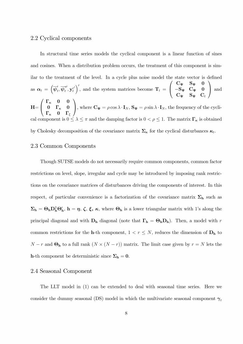
2.2 Cyclical components

In structural time series models the cyclical component is a linear function of sines

and cosines. When a distribution problem occurs, the treatment of this component is sim-

ilar to the treatment of the level. In a cycle plus noise model the state vector is defined

as αt =³ψ0t,ψ

∗0t ,y

c0t

´0, and the system matrices become Tt =

CΨ SΨ 0−SΨ CΨ 0CΨ SΨ Ct

and

H=

Γκ 0 00 Γκ 0Γκ 0 Γξ

, where CΨ = ρ cosλ · IN , SΨ = ρ sinλ · IN , the frequency of the cycli-

cal component is 0 ≤ λ ≤ π and the damping factor is 0 < ρ ≤ 1. The matrix Γκ is obtained

by Cholesky decomposition of the covariance matrix Σκ for the cyclical disturbances κt.

2.3 Common Components

Though SUTSE models do not necessarily require common components, common factor

restrictions on level, slope, irregular and cycle may be introduced by imposing rank restric-

tions on the covariance matrices of disturbances driving the components of interest. In this

respect, of particular convenience is a factorization of the covariance matrix Σh such as

Σh = ΘhD2hΘ

0h, h = η, ζ, ξ, κ, where Θh is a lower triangular matrix with 1’s along the

principal diagonal and with Dh diagonal (note that Γh = ΘhDh). Then, a model with r

common restrictions for the h-th component, 1 < r ≤ N , reduces the dimension of Dh to

N − r and Θh to a full rank (N × (N − r)) matrix. The limit case given by r = N lets the

h-th component be deterministic since Σh = 0.

2.4 Seasonal Component

The LLT model in (1) can be extended to deal with seasonal time series. Here we

consider the dummy seasonal (DS) model in which the multivariate seasonal component γt

8

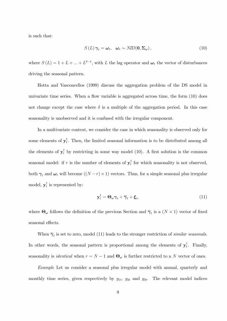
is such that:

S (L)γt = ωt, ωt ∼ NID(0,Σω) , (10)

where S (L) = 1 +L+ ...+Lδ−1, with L the lag operator and ωt the vector of disturbances

driving the seasonal pattern.

Hotta and Vasconcellos (1999) discuss the aggregation problem of the DS model in

univariate time series. When a flow variable is aggregated across time, the form (10) does

not change except the case where δ is a multiple of the aggregation period. In this case

seasonality is unobserved and it is confused with the irregular component.

In a multivariate context, we consider the case in which seasonality is observed only for

some elements of y†t . Then, the limited seasonal information is to be distributed among all

the elements of y†t by restricting in some way model (10). A first solution is the common

seasonal model: if r is the number of elements of y†t for which seasonality is not observed,

both γt and ωt will become ((N − r)× 1) vectors. Thus, for a simple seasonal plus irregular

model, y†t is represented by:

y†t = Θωγt + γt + ξt, (11)

where Θω follows the definition of the previous Section and γt is a (N × 1) vector of fixed

seasonal effects.

When γt is set to zero, model (11) leads to the stronger restriction of similar seasonals.

In other words, the seasonal pattern is proportional among the elements of y†t . Finally,

seasonality is identical when r = N − 1 and Θω is further restricted to a N vector of ones.

Example Let us consider a seasonal plus irregular model with annual, quarterly and

monthly time series, given respectively by y1t, y2t and y3t. The relevant model indices

9

are N = 3, δ = 12, δ+1 = 1, δ+2 = 4 and δ+3 = 12. Since seasonality is fully observed

for the first series only, one disturbance drives the stochastic seasonal component. Then,

imposing similar seasonals the state vector is αt =¡γt, γt−1, ..., γt−10,y

c0t

¢0and the system

matrices Tt and H are Tt =

µTγ 0Zγ Ct

¶, H =

µHγ 00 Γξ

¶and Tγ =

µ −1011I10 0

¶, with

Hγ = diag(σω, 010), Zγ = Θω ⊗ e11 and Θω = (1, θω2, θω3)0; 1m and 0m denote m−vectors

of ones and zeros respectively, and em is the first row of the identity matrix Im.

3. COMPARISON WITH OTHER METHODS

The main methods for temporal disaggregation proposed by the literature hypothesize

a simple linear univariate relationship between the unknown low-frequency variable y1t and

the high-frequency related time series y2t. The most important difference among the various

methods lies in the structure imposed on the residuals of the hypothesized econometric

relationship. Starting from the high frequency variables regression, y1t = α+ βy2t + ut, the

key issue - after temporal aggregation and estimation of the model with observed series - is

the identification of the covariance matrix of the disturbances of the high frequency model

from the estimated covariance matrix of the low-frequency model. This model is derived

from the available low-frequency data, possibly by imposing an ARIMA structure on the

data generating process of ut | y2t. In particular, it is assumed to be an AR(1) process by

Chow and Lin (1971), an I(1) process by Fernández (1981), and an ARIMA(1, 1, 0) process

by Litterman (1983). Though the proposal of Stram and Wei (1986) encompasses the other

models, as it considers a general ARIMA(p, d, q) structure of the data generation process

of the aggregated series and, if an indicator is available, an ARIMA(p, d, q) model for the

residuals, NSI’s often limit their consideration to the Chow and Lin’s family of procedures

10

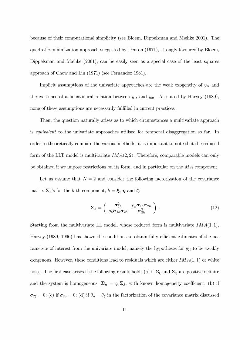
because of their computational simplicity (see Bloem, Dippelsman and Mæhke 2001). The

quadratic minimization approach suggested by Denton (1971), strongly favoured by Bloem,

Dippelsman and Mæhke (2001), can be easily seen as a special case of the least squares

approach of Chow and Lin (1971) (see Fernández 1981).

Implicit assumptions of the univariate approaches are the weak exogeneity of y2t and

the existence of a behavioural relation between y1t and y2t. As stated by Harvey (1989),

none of these assumptions are necessarily fulfilled in current practices.

Then, the question naturally arises as to which circumstances a multivariate approach

is equivalent to the univariate approaches utilised for temporal disaggregation so far. In

order to theoretically compare the various methods, it is important to note that the reduced

form of the LLT model is multivariate IMA(2, 2). Therefore, comparable models can only

be obtained if we impose restrictions on its form, and in particular on the MA component.

Let us assume that N = 2 and consider the following factorization of the covariance

matrix Σh’s for the h-th component, h = ξ, η and ζ:

Σh =

µσ21h ρhσ1hσ2h

ρhσ1hσ2h σ22h

¶. (12)

Starting from the multivariate LL model, whose reduced form is multivariate IMA(1, 1),

Harvey (1989, 1996) has shown the conditions to obtain fully efficient estimates of the pa-

rameters of interest from the univariate model, namely the hypotheses for y2t to be weakly

exogenous. However, these conditions lead to residuals which are either IMA(1, 1) or white

noise. The first case arises if the following results hold: (a) if Σξ and Ση are positive definite

and the system is homogeneous, Ση = qηΣξ, with known homogeneity coefficient; (b) if

σ2ξ = 0; (c) if σ2η = 0; (d) if θη = θξ in the factorization of the covariance matrix discussed

11

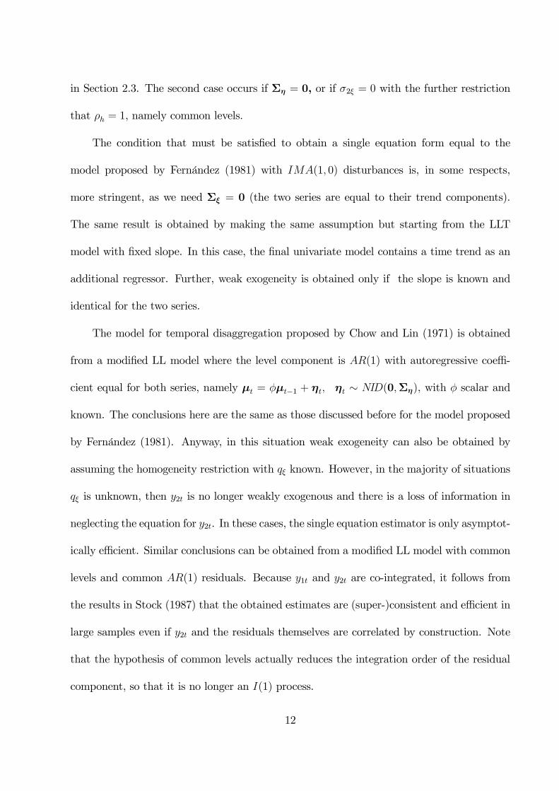
in Section 2.3. The second case occurs if Ση = 0, or if σ2ξ = 0 with the further restriction

that ρh = 1, namely common levels.

The condition that must be satisfied to obtain a single equation form equal to the

model proposed by Fernández (1981) with IMA(1, 0) disturbances is, in some respects,

more stringent, as we need Σξ = 0 (the two series are equal to their trend components).

The same result is obtained by making the same assumption but starting from the LLT

model with fixed slope. In this case, the final univariate model contains a time trend as an

additional regressor. Further, weak exogeneity is obtained only if the slope is known and

identical for the two series.

The model for temporal disaggregation proposed by Chow and Lin (1971) is obtained

from a modified LL model where the level component is AR(1) with autoregressive coeffi-

cient equal for both series, namely µt = φµt−1 + ηt, ηt ∼ NID(0,Ση), with φ scalar and

known. The conclusions here are the same as those discussed before for the model proposed

by Fernández (1981). Anyway, in this situation weak exogeneity can also be obtained by

assuming the homogeneity restriction with qξ known. However, in the majority of situations

qξ is unknown, then y2t is no longer weakly exogenous and there is a loss of information in

neglecting the equation for y2t. In these cases, the single equation estimator is only asymptot-

ically efficient. Similar conclusions can be obtained from a modified LL model with common

levels and common AR(1) residuals. Because y1t and y2t are co-integrated, it follows from

the results in Stock (1987) that the obtained estimates are (super-)consistent and efficient in

large samples even if y2t and the residuals themselves are correlated by construction. Note

that the hypothesis of common levels actually reduces the integration order of the residual

component, so that it is no longer an I(1) process.

12

If the starting point is the modified LLT model with autoregressive slopes and Σξ = 0,

weak exogeneity is obtained if the model is trend homogeneous, Σζ = qζΣη , with qη known.

Furthermore, as stated before, unless the autoregressive parameters are equal in the two

equations and known, there is a loss of efficiency in parameters estimates if these are based

on single equation estimation. In other words, we do not have weak exogeneity. Anyway, the

resulting residuals of the single equation for y1t are ARIMA(1, 1, 1): then, the model adds

to the residual of the model proposed by Litterman (1983) a moving average component,

and can be judged as more close to the wider assumptions of the approach by Stram and

Wei (1986) and Wei and Stram (1990).

It should be noted that the assumptions of common levels and slopes, even whenΣξ = 0,

do not lead us to obtain weak exogeneity for y2t in the equation of interest. Therefore,

according to what stated for the model by Fernández (1981), also the model favoured by

Litterman (1983) is in conflict with the likely property in this context of co-integration

between y1t and y2t.

4. RESULTS OF THE EMPIRICAL ANALYSES

In this Section we compare the results obtained by applying the structural approach

with those obtained from the main methods for temporal disaggregation proposed so far by

the literature and discussed in Section 3. The results of the structural approach have been

generated using the Ox program, version 3.0 (see Doornik 2001), and the SsfPack package

(see Koopman, Shephard and Doornik 2002), while for the other methods we have benefited

from the program Ecotrim developed by Eurostat (see Eurostat 1999).

4.1 The data set used for comparisons

13

The comparisons are carried out by considering a wide data set drawn from OECD

(2002). The time series chosen refer to the twelve biggest OECD countries in terms of Gross

Domestic Product (GDP) at current prices in 2001. Eight sets of data are used: 1) Industrial

production index and deliveries in manufacturing; 2) GDP and industrial production index;

3) Consumer and producer price indices; 4) Private consumption and GDP; 5) GDP deflator

and consumer price index; 6) Broad and narrow money supply; 7) Short-term and long-term

interest rates; 8) Imports evaluated on a f.o.b. (free on board) and c.i.f. (costs, insurances

and freights) basis. In total, we have 96 cases considered (8 data sets times 12 countries).

Whenever available in the OECD data set, unadjusted data have been preferred to the

corresponding seasonally adjusted series. The eight sets of data have been chosen in order

to cover almost all the various situations which typically occur in practice. In particular, in

case 6) we have an interpolation problem (stock variables, last observation of the reference

period as benchmark), while in the other cases we face a distribution problem (index series in

all cases but 8), where a distribution of flow variables is considered). As regards frequencies,

the following cases are considered: a disaggregation problem from quarterly to monthly

observations, δi = 3, in cases 1), 3) and 6); from annual to quarterly in cases 2), 3), 4) and

8); and from annual to monthly in case 7). Following the terminology used for the univariate

framework, the related series is the second series indicated in every set of data, whilst the

first series is the ‘dependent’ variable.

Once the results of the disaggregations have been obtained for all the methods, they

can be compared with the actual data using standard statistics, such as root mean squared

or mean absolute errors. In what follows, we report the results obtained in terms of root

mean squared percentage errors (RMSPE) only to save space. The results obtained with

14

other criteria, available upon request, do not change the ordering of the results and the

conclusions reported below.

Though the related series have been chosen on an ad hoc basis so as to be the closest

approximation to the dependent variable in the data set, nonetheless a variety of situations

arise in our experiments. In some cases, the related series are very close to the target

variable, both as concerns their meaning and time-series properties. This is the case of

experiment 8), where the c.i.f and f.o.b evaluations of imports differ only for insurance and

freight charges. In other cases, though the related series is part of the dependent series,

the two variables can substantially differ as a consequence, for example, of the increasing

importance of new forms of payment, such as in case 6), or different short and long-term

elasticities to economic conditions and expectations, such as in case 7). In some experiments

the variables are casually linked (cases 1), 3) and 4)), while in others they are only subject

to a similar economic environment and simply measure similar things (cases 2) and 5)). The

heterogeneity in the data set used is further increased by countries’ specificities.

4.2 Testing in the SUTSE model

One of the main advantages of the proposed approach is that it does not impose any a

priori structure on the data. The final model depends on the stochastic behavior of the data

and on their representation in terms of univariate/multivariate structural time series model.

Unobserved components may assume a variety of forms and common component restrictions

may be imposed, whenever appropriate, in a very straightforward and natural way. In this

respect, an important question to be addressed regards the form of the trend component and

the determination of whether common factor restrictions can be imposed. However, though

common factors are desirable in our context, SUTSE models only impose them as special

15

cases and the SUTSE approach can give gains from using related indicators even if there are

significant differences in the time behaviour of the related and the target series, for example

a tendency of one series in the system to drift apart (see Harvey and Chung, 2000).This

aspect will be further clarified below.

Given that most of the time-series in our data set show a clear upward trend, our

preferred approach consists in starting from the general multivariate LLT model, augmented

to include seasonal and cyclical components whenever appropriate.

Concerning the seasonal component, two situations can arise: a) the component is

observed only for the high frequency series; b) the component is observed with different

frequencies on both series. In the first case, our choice has been either to use, whenever

feasible, the information drawn from the estimate of the factor loading of the level, or to

impose identical seasonality when the levels of the series are compatible. In the latter case,

one can also consider the information on the seasonal factor loading estimated from the

low-frequency model.

Once a first estimation is run, some of the variances of the system in the general LLT

model can be fixed by the system estimation itself because approximately equal to zero.

The literature has recently proposed a number of tests for the form of the trend compo-

nent and for the existence of common factors (see Nyblom and Harvey 2000, 2001). However,

in general it is not possible to represent the observed aggregated series by a fully orthogonal

structural model (see Harvey 1989; Hotta and Vasconcellos 1999). This could invalidate the

use of the non parametric versions of these tests. One possible solution, adopted in the dis-

aggregations discussed below, consists in using parametric versions of the tests based on the

innovations obtained from the model estimated at the lower frequency the series are observed

16

(see, e.g., Harvey 2001; Nyblom and Harvey 2000, 2001). These tests start from estimat-

ing the nuisance parameters of the unrestricted model, then follow in running the Kalman

filter and smoother with the appropriate variances set to zero to extract the innovations or

‘smoothing errors’, and to construct tests which have the same asymptotic properties and

more reliable size in small samples (see Nyblom and Harvey 2001).

In the LL model, a test for the null hypothesis that Ση = 0 against the homo-

geneous alternative Ση = qΣξ, q > 0, is given by η(r,N) = tr (S−1C), with C =

n−2Pn

i=1

³Pit=1 νt

´³Pit=1 νt

´0, S = n−1

Pnt=1 νtν

0t and νt the Kalman filter estimated

residuals. In the LLT with constant slope, the test above is indicated with η0(r,N),

with different rejection regions from η(r,N). In the IRW model, the test for Σζ = 0

against the homogeneous alternative Σζ = qΣξ is given by ζ = tr (S−1T), where T =

n−2Pn

i=1

hPis=1

Psr=1 νt

i hPis=1

Psr=1 ν

0t

i(see Nyblom and Harvey 2001). Finally, the test

against a stochastic slope with Ση > 0 is again given by η(r,N).

Furthermore, we might test for a specified number r of common levels/slopes, that is

we might test for the rank of the relevant covariance disturbance. The test is constructed on

the sum of the N − r smallest eigenvalues of the matrices constructed on the innovations.

4.3 Results of comparison

As an illustrative example of the proposed disaggregation method, we consider the quar-

terly GDP and the industrial production index for the US. The series are seasonally adjusted

and cover the sample period 1960.q1-2002.q1 (n = 169). Data on GDP are firstly annually

aggregated and then quarterly disaggregated using a multivariate LLT model. Given the

17

factorization (12), we have obtained the following estimates:

eσ1η = 26.1 eσ2η = 11.2 eρη = 0.292eσ1ζ = 22.3 eσ2ζ = 13.3 eρζ = 0.997eσ1ξ = 0.252,with the irregular component of the second series eσ2ξ equal to zero, and consequently eρξ = 0.Concerning GDP, the diagnostics based on innovations are Q(6) = 2.75 and NORM = 0.72,

while for the production index are Q(13) = 37.45 and NORM = 43.69, where Q (P ) is the

Box-Ljung statistic based on the P autocorrelations and NORM is the Bowman-Shenton

normality test statistic based on skewness and kurtosis of residuals. If the model is correctly

specified, the Box-Ljung statistics are asymptotically distributed with P − 1 degrees of

freedom, whereas NORM is distributed as a χ2 with 2 degrees of freedom. There is no

evidence of serial correlation and non normality in the GDP residuals, while this is the case for

the production index, possibly because of large changes in the series not completely reflected

in GDP data. This is a feature our structural model shares with the other competitors. For

example, the second best solution in our experiments is the Litterman’s model (see Table 1),

where we have a Ljung Box Q-statistic of the residuals in the annual relation at lag 7 equal

to 34.94. Recently, the literature has shown the existence of different forms of non linearities

in the US industrial production index, due for example to outliers, asymmetries in business

cycle movements and time irreversibility. When seasonal unadjusted data are used, as in the

example considered below, serial correlation and non normalities can also emerge as a result

of either of seasonal heteroscedasticity and trends, or different seasonal behaviour between

the target and the related series. Structural models can be amended in a number of ways to

obtain better fits in these circumstances (see Proietti 1999, and for the seasonal case, Proietti

1998). The use of logarithms or other transformations of the original series could add to

18

the fit of the structural model, but can create relevant problems, particularly for temporal

disaggregations of flow series. We do not address these relevant issues in the present context.

The important point to make here is that the structural approach still works properly even

though the fit we obtain is not entirely satisfactory.

The results of the quarterly disaggregation of GDP have been compared with the actual

quarterly data to obtain a RMSPE equal to 0.355. The estimates indicate the existence of

a common slope (η (1, 2) is equal to 0.075, well below the 5% critical value of 0.218) and an

irregular component approximately equal to zero. Imposing such restrictions does not change

final results and the diagnostics reported above. The gains from using an indicator series in

the structural approach are substantial, as clearly emerges from comparing the results here

obtained with those of the univariate model, for which the RMSPE is equal to 0.465 (see

Table 1). As noted by Harvey and Chung (2000), this may be due to the fact that, though

the slopes of the two series are highly correlated, the two levels show a tendency to drift

apart, possibly as a consequence of the decreasing contribution of the industrial sector to

total GDP. This evidence shows that a high correlation between the disturbances in the two

series - and hence the existence of common factors - not necessarily leads to big increases in

the accuracy of final estimates.

The LLT model could also be estimated with a cyclical component. In this respect, an

interesting question concerns whether its inclusion adds something to the accuracy of the

model. An alternative specification, in line with the findings in Harvey and Jeager (1993)

for US quarterly GNP, is the IRW model plus a cyclical component. The results are:

eσ1ζ = 14.3 eσ2ζ = 8.0 eρζ = 0.973eσ1κ = 20.9 eσ2κ = 11.3 eρκ = 0.739,19

with eσ1ξ = eσ1ξ = 0 and the cyclical period equal to 12.5 quarters. The diagnostics are

Q(6) = 2.13 and NORM = 0.18 for GDP and Q(13) = 32.44 and NORM = 29.11 for the

index of production, somewhat below those of the complete system. The RMSPE of the

disaggregation model is equal to 0.351, a result very close to that obtained from the LLT

model. The ζ-test, equal to 28.5, clearly rejects the null of a deterministic slope. Similar

results are obtained for Spain, where the inclusion of the cyclical component reduces the

RMSPE with respect to the LLT model with common slope of only 0.5%.

As a second example, we consider the quarterly aggregated industrial production index

and monthly revenues for Germany in the sample 1991.m1-2002.m3 (n = 135). As the series

are seasonally unadjusted, we start from the LLT model plus a seasonal component. The

results are: eσ1η = 1.111 eσ2η = 1.538 eρη = 1.000eσ1ζ = 0.069 eσ2ζ = 0.078 eρζ = 1.000eσ1ω = 0.319 eσ2ω = 0.319 eρω = 1.000eσ1ξ = 2.532 eσ2ξ = 4.286 eρξ = −1.000.The diagnostics for the production index areQ(6) = 14.35 andNORM = 14.79, for deliveries

we obtained Q(11) = 43.15 and NORM = 0.69. The RMSPE is equal to 2.328. Common

restrictions on level and slope are naturally obtained by numerical optimization, in line with

the results given by the test η (1, 2) on the slope component, equal to 0.046.

Considering the general results in terms of RMSPE, presented in Table 1 for the 96 ex-

amples, they indicate that the multivariate structural approach is likely to be more accurate

than the other methods in virtually all the distributions of time series. Table 2 shows that

the SUTSE approach has a percentage of success over the competitors which varies from

about 78% (against the univariate structural model) to about 92% (against the Chow-Lin’s

approach). For all the experiments, the average gain in terms of RMSPE varies from about

20

14% in the case of the Litterman’s procedure, to some 60% for the Denton’s model. Among

the methods using related time series, the approach by Litterman seems to be, on average,

the second-best solution for time disaggregation issues. This is probably due to the fact that

this approach is the closest to the SUTSE approach because, on the one hand, it requires

less restrictions on the form of the underlying multivariate system, as noted before, and on

the other hand it is more able to resemble the time behaviour of highly non-stationary time

series. Almost at the same level, the approaches by Denton (1971) and Chow and Lin (1971)

have quite unsatisfactory performances with respect to the other methods: their probabili-

ties of success, even against methods which do not use related time series, is seldom above

0.4.

When no indicator is available, the best solution seems again to be offered by the use of

a structural approach, with a gain in terms of accuracy over the approaches by Denton and

Stram-Wei of about 15%. Another interesting result emerges from our experiments. Coeteris

paribus, the use of a related series can have an impact on accuracy of final estimates which

greatly depends on the method used for time disaggregation. In fact, while the gains obtained

passing from the univariate structural model to the SUTSE approach are substantial (about

35%, with an increase of the probability of success of 22%), for the Denton’s approach

the use of a related time series seems to even worsen the final outcomes (a reduction of

3% in accuracy, with a probability of success of about 33%). Therefore, what this limited

experiment seems to indicate is that the choice of the method for time disaggregation can be

even more relevant than the use of a good reference series, even if the use of this series can add

substantially in terms of accuracy when an appropriate framework for time disaggregation is

chosen. Furthermore, as noted before, the gains from using the SUTSE over the univariate

21

structural approach can be low when the series show similar behaviour. This is what emerges

from cases C and E in our data set where, on average, the target and the related series are

characterised by similar patterns. Here the gains in terms of RMSPE from using an indicator

series is of 2.4% (against an average of 35.1% in the whole data set) and the probability of

success reduces to 62.5% from an average of 78.1%.

Table 3 shows, for each experiment, the sample, the final model estimated and the

results obtained from the parametric tests discussed above. It can be noted that in 58 over

96 cases the LBI tests confirm the appropriateness of the model finally chosen. The models

contain stochastic levels without common factor restrictions in the majority of cases (75 over

96), and in about 50% of these models the slopes of both the indicator and the target series

are deterministic. In fifteen cases we obtained a complete LLT model without restrictions,

whilst in eleven cases the more appropriate model includes both common levels and slopes.

The other preferred models account for the other twelve cases. A cycle is added in only two

final models and the gains obtained are rather weak, as discussed before. In the cases where

a seasonal component is needed, the proportional form has always been imposed. Regarding

the monthly disaggregation of prices, we have found that in most experiments the seasonal

component in both series is well described by a deterministic dummy component.

5. SUMMARY AND LINES FOR FUTURE RESEARCH

This paper describes a framework for time disaggregation of time series based on struc-

tural multivariate models. The approach here suggested has the advantage over the main

competitors that it does not impose any particular structure on the data, and it is flexible

enough to fit almost any temporal disaggregation problem. Furthermore, it easily allows for

22

common factor restrictions among components, a quite natural circumstance which is not

fully taken into account by other methods. We have shown that only under very particu-

lar conditions, usually not met in practice, the SUTSE approach reduces to the univariate

methods mostly used in current practice by NSI’s. The results of our experiments, which use

a large number of time series covering almost all the various situations typically occurring

in real life, show that the gains from using the multivariate/univariate structural approach

can be substantial.

A feasible line for future research is the use of a logarithmic transformation for the

variables characterised by increasing trends and variances. That could have some impact on

the model chosen on the basis of the parametric tests used in this paper, and could improve

diagnostics. Though modelling the series in logs creates no difficulties for stock variables,

for flow series no simple solution exists at the moment simply because, for the aggregated

variable, the logarithm of the sum is not equal to the sum of the logarithms. As suggested in

Harvey and Pierce (1984), one way to proceed would be to assume that the logarithms of the

variables are normally distributed, then to modify accordingly the state-space representation

of the model, and finally to use the extended Kalman filter to obtain an approximation to

the likelihood function computed by the prediction error decomposition.

Model selection strategy when observations are missing is another important issue to

be further investigated. In this paper we have followed a ‘reduction strategy’ based on the

results of parametric tests available in the literature. Advances in this field will certainly

add to the choice of the final model for time disaggregation.

23

REFERENCES

Bloem, A. M., Dippelsman, R. J., and Mæhke, N. Ø. (2001), Quarterly National Accounts

Manual - Concepts, Data Sources, and Compilation, International Monetary Fund,

Washington DC.

Chow, G., C., and Lin, A. (1971), “Best Linear Unbiased Interpolation, Distribution and Ex-

trapolation of Time Series by Related Series,” The Review of Economics and Statistics,

53, 372-375.

Denton, F. T. (1971), “Adjustment of Monthly or Quarterly Series to Annual Totals: An

Approach Based on Quadratic Minimization,” Journal of the American Statistical As-

sociation, 66, 99-102.

Doornik, J. A. (2001), Ox 3.0 - An Object-Oriented Matrix Programming Language, London:

Timberlake Consultants Ltd.

Durbin J. and Quenneville, B. (1997), “Benchmarking by State Space Models,” International

Statistical Review, 65, 23-48.

Eurostat (1999), Handbook on Quarterly National Accounts, Luxembourg: European Com-

munities.

Fernández, R. B. (1981), “A Methodological Note on the Estimation of Time Series,” The

Review of Economics and Statistics, 63, 471-476.

Fernández, F. J., and Harvey, A. C. (1990), “Seemingly Unrelated Time Series Equations

and a Test for Homogeneity,” Journal of Business & Economic Statistics, 8, 71-81.

Harvey, A. C. (1989), Forecasting, Structural Time Series Models and the Kalman Filter,

Cambridge: Cambridge University Press.

24

(1996), “Intervention Analysis with Control Groups,” International Statistical Re-

view, 64, 313-328.

(2001), “Testing in Unobserved Components Models,” Journal of Forecasting, 20,

1-19.

Harvey, A. C., and Chung, C. (2000), “Estimating the Underlying Change in Unemployment

in the UK,” Journal of the Royal Statistical Society A, 163, 303-339.

Harvey, A. C., and Jaeger, A. (1993), “Detrending, Stylized Facts and the Business Cycle,”

Journal of Applied Econometrics, 8, 231-247.

Harvey, A. C., and Koopman, S. J. (1997), “Multivariate Structural Time Series Models”

(with comments), in System Dynamics in Economic and Financial Models, eds C. Heij,

J. M. Shumacher, B. Hanzon and C. Praagman, Chichester: John Wiley & Sons Ltd,

pp. 269-298.

Harvey, A. C., and Pierce, R. G. (1984), “Estimating Missing Observations in Economic

Time Series,” Journal of the American Statistical Association, 79, 125-131.

Hotta, L. K., and Vasconcellos, K. L. (1999), “Aggregation and Disaggregation of Structural

Time Series Models,” Journal of Time Series Analysis, 20, 155-171.

Koopman, S. J., (1997), “Exact Initial Kalman Filtering and Smoothing for Non-Stationary

Time Series Models,” Journal of the American Statistical Association, 92, 1630-1638.

Koopman, S. J., and Durbin, J. (1999), “Filtering and Smoothing of State Vector for Diffuse

State Space Models,” mimeo, July.

(2000), “Fast Filtering and Smoothing for Multivariate State Space Models,” Journal

of Time Series Analysis, 21, 281-96.

Koopman, S. J., Shephard, N., and Doornik, J. A. (2002), “SsfPack 3.0beta02: Statistical

Algorithms for Models in State Space,” February.

25

Litterman, R. B. (1983), “A Random Walk, Markov Model for Distribution of Time Series,”

Journal of Business & Economic Statistics, 1, 169-173.

Nyblom, J., and Harvey, A. C. (2000), “Tests of Common Stochastic Trends,” Econometric

Theory, 16, 176-199.

(2001), “Testing Against Smooth Stochastic Trends,” Journal of Applied Economet-

rics, 16, 415-429.

OECD (2002), Main Economic Indicators, Paris, July.

Proietti, T. (1998), “Seasonal Heteroscedasticity and Trends,” Journal of Forecasting, 17,

1-17.

(1999), “Characterising Asymmetries in Business Cycles Using Smooth Transition

Structural Time Series Models,” Studies in Nonlinear Dynamics and Econometrics, 3,

141-156.

Stock, J. H. (1987), “Asymptotic Properties of Least Squares Estimators of Co-Integrating

Vectors,” Econometrica, 55, 1035-1056.

Stram, D. O., and Wei, W. W. S. (1986), “A Methodological Note on the Disaggregation of

Time Series Totals,” Journal of Time Series Analysis, 7, 293-302.

Wei, W. W. S., and Stram, D. O. (1990), “Disaggregation of Time Series Models,” Journal

of the Royal Statistical Society, Series B, 52, 453-467.

26

Table 1. Results of time disaggregations: root mean square percentage errors (RMSPE)

COUNTRY Can Mex Usa Aus∗ Jap Kor Fra Deu Ita Nld Esp Gbr

A. Quarterly industrial production - Monthly deliveriesSUTSE 3.017 2.643 0.919 4.008 3.189 3.379 11.118 2.328 6.017 5.901 14.573 6.052Chow-Lin 3.284 2.855 0.877 3.878 4.673 4.426 10.075 3.206 6.535 6.324 14.794 6.988Fernández 3.381 2.851 0.887 3.010 4.773 3.517 9.992 7.831 6.814 6.008 14.798 6.540Litterman 3.456 2.857 1.031 6.415 4.951 4.098 10.970 11.593 6.711 6.510 15.066 6.824Denton 3.325 4.728 2.899 5.271 19.222 13.098 12.363 3.350 6.998 7.089 14.901 11.380

Structural 5.389 2.990 2.077 4.146 4.395 3.375 8.906 5.264 23.276 4.349 14.939 5.534Denton 5.579 2.990 2.078 4.170 4.468 3.389 8.906 5.265 23.276 4.350 14.936 5.534Stram-Wei 5.549 3.009 2.073 4.159 4.459 3.460 9.178 5.332 23.947 5.856 15.289 5.487

B. Annual GDP - Quarterly industrial productionSUTSE 0.202 2.244 0.351 0.513 0.484 0.561 0.221 0.347 0.484 0.509 0.456 0.474Chow-Lin 0.213 2.287 0.751 1.214 0.648 0.683 0.670 0.431 0.604 1.856 0.942 1.486Fernández 0.214 2.249 0.452 0.855 0.559 0.606 0.367 0.367 0.604 0.793 0.502 0.599Litterman 0.213 2.245 0.358 0.613 0.495 0.633 0.256 0.369 0.504 0.509 0.454 0.457Denton 0.205 2.329 0.718 0.984 1.031 0.877 0.536 0.745 1.208 1.069 0.716 0.882


C. Quarterly consumer prices - Monthly producer pricesSUTSE 0.209 3.115 0.161 0.460 0.323 0.229 0.191 0.161 0.112 0.253 0.519 0.349Chow-Lin 0.317 5.279 0.341 0.671 0.347 0.296 0.443 0.199 0.271 0.278 0.798 0.396Fernández 0.236 3.499 0.200 0.610 0.335 0.236 0.240 0.163 0.170 0.265 0.594 0.379Litterman 0.215 3.310 0.158 0.469 0.334 0.241 0.190 0.161 0.114 0.279 0.478 0.395Denton 0.300 3.146 0.317 0.593 0.355 0.266 0.349 0.177 0.196 0.310 0.543 0.370


D. Annual private consumption expenditures- Quarterly GDPSUTSE 0.345 2.552 0.314 0.494 0.579 1.243 0.309 0.567 0.495 0.500 0.528 0.553Chow-Lin 0.393 2.812 0.465 0.869 0.479 1.105 0.328 0.587 0.639 0.582 0.572 0.653Fernández 0.372 2.863 0.434 0.777 0.510 1.173 0.309 0.533 0.572 0.597 0.586 0.617Litterman 0.384 2.889 0.333 0.518 0.635 1.314 0.317 0.594 0.441 0.530 0.647 0.554Denton 0.401 2.756 0.442 0.901 0.472 1.202 0.295 0.556 0.563 0.635 0.603 0.586


NOTE: Legenda - Can=Canada, Mex=Mexico, USA=The United States of America,Aus=Australia, Jap=Japan, Kor=North Korea, Fra=France, Deu=Germany, Ita=Italy,Nld=Netherlands, Esp=Spain, Gbr=Great Britain. ∗In cases A and C annual-quarterly exerciseinstead of quarterly-monthly.

27

Table 1 (follows). Results of time disaggregations: RMSPE

COUNTRY Can Mex Usa Aus Jap Kor Fra Deu Ita Nld Esp Gbr

E. Annual GDP deflator - Quarterly consumer prices

SUTSE 0.310 6.321 0.170 0.901 0.217 0.850 0.434 0.261 0.585 0.371 0.333 0.492Chow-Lin 0.330 11.474 0.211 0.999 0.224 0.856 0.450 0.340 0.621 0.379 0.440 0.759Fernández 0.308 6.716 0.205 0.976 0.250 0.854 0.455 0.364 0.624 0.384 0.409 0.743Litterman 0.266 7.004 0.178 0.930 0.248 0.841 0.437 0.341 0.604 0.383 0.396 0.532Denton 0.325 6.619 0.233 1.001 0.272 0.846 0.457 0.389 0.604 0.395 0.384 0.747


F. Quarterly broad money supply - Monthly narrow money supply



G. Annual short-term interest rates - Monthly long-term interest rates



H. Annual imports c.i.f. - Quarterly imports f.o.b.



28

Table 2. Synthesis of the results obtained in terms of RMSPE

METHODS SUTSE Chow- Fernández Litterman Denton Structural Denton Stram-Lin univ. Wei

SUTSE - 147.2 123.1 114.3 158.8 135.1 154.1 155.4Chow-Lin 91.7 - 83.6 77.7 107.9 92.1 104.7 105.6Fernández 86.5 26.0 - 92.9 129.0 110.1 125.2 126.2Litterman 81.3 31.3 41.7 - 138.8 118.5 134.7 135.9Denton 88.5 52.1 71.9 71.9 - 85.4 97.1 97.9

Structural 78.1 36.5 45.8 54.2 33.3 - 113.7 114.7Denton univ. 82.3 41.7 57.3 62.5 36.5 76.0 - 100.8Stram-Wei 83.3 43.8 59.4 65.6 36.5 79.2 59.4 -

NOTE: The Table shows, in the lower part, the percentage of success of the method incolumn over that in row, in the upper part the geometric average of the ratios of RMSPEof the method in column over the method in row. A geometric mean is used for itsreciprocity properties.

29

Table 3. Results and synthesis of the SUTSE models


A. Quarterly industrial production - Monthly deliveries

n 495 195 507 72 507 147 327 135 255 375 86 507Order (2,0,1) (2,1,2) (2,0,1) (2,0,1) (2,1,2) (2,1,2) (2,0,2) (1,1,1) (2,0,1) (2,0,1) (2,1,0) (2,1,2)Seasonal 1 0 1 1 1 1 1 1 1 1 0 1η0 (1, 2) 0.951 - 1.058 0.209 - - 1.392 - 0.377 2.216 - -η0 (0, 2) 3.974 - 14.708 0.986 - - 3.473 - 6.930 4.591 - -η (1, 2) - 0.062 - - 0.107 0.153 - 0.046 - - 0.223 0.143η (0, 2) - 1.910 - - 1.515 0.656 - 1.893 - - 2.033 0.471ζ 35.809 26.213 83.026 10.642 5.793 23.267 63.524 33.790 118.60 40.202 59.643 119.56

B. Annual GDP - Quarterly industrial production

n 85 88 169 108 88 53 97 45 129 101 89 169Order (2,1,0) (2,0,0) (0,2,0) (1,1,1) (1,1,2) (2,0,0) (2,0,1) (2,0,0) (2,0,0) (1,1,1) (0,2,0) (2,1,0)Cycle × × 2 × × × × × × × 2 ×η0 (1, 2) - 0.418 - - - 0.044 - 0.044 0.031 - - -η0 (0, 2) - 6.978 - - - 0.525 - 1.390 0.190 - - -η (1, 2) 0.166 - 0.075 0.302 0.173 - 0.178 - - 0.049 0.069 0.048η (0, 2) 1.283 - 1.706 7.317 0.645 - 0.406 - - 0.916 3.218 1.290ζ 4.889 52.679 28.471 170.03 12.326 - 4.357 2.478 5.163 5.361 55.941 43.925

C. Quarterly consumer prices - Monthly producer prices

n 508 256 508 133 388 160 508 508 256 316 508 508Order (2,2,0) (2,2,1) (2,2,0) (2,1,0) (2,0,0) (2,0,0) (0,2,0) (2,0,1) (2,0,0) (2,2,1) (2,2,1) (2,0,2)Seasonal 0 1 0 × 0 0 × 0 0 1 0 0η0 (1, 2) - - - - 0.185 0.052 - 0.492 0.181 - - 0.236η0 (0, 2) - - - - 3.500 1.531 - 6.981 7.588 - - 17.310η (1, 2) 0.411 0.294 0.577 0.132 - - 0.098 - - 0.250 0.752 -η (0, 2) 6.018 6.467 21.573 2.948 - - 5.225 - - 4.700 23.869 -ζ 101.84 15.586 284.57 42.79 29.010 11.261 230.92 261.38 135.97 108.26 171.06 244.08

D. Annual private consumption expenditures - Quarterly GDP

n 85 88 169 168 88 129 97 45 128 101 89 169Order (2,1,2) (2,0,0) (2,1,2) (2,1,1) (2,0,0) (2,0,0) (2,0,0) (2,0,0) (2,0,0) (2,1,0) (2,1,1) (2,1,0)η0 (1, 2) - 0.106 - - 0.138 0.057 0.169 0.179 0.247 - - -η0 (0, 2) - 0.486 - - 0.576 1.850 0.966 1.139 2.303 - - -η (1, 2) 0.228 - 0.061 0.050 - - - - - 0.089 0.109 0.061η (0, 2) 1.384 - 1.306 1.773 - - - - - 0.470 2.081 0.923ζ 13.792 47.714 25.197 14.376 13.481 17.307 4.718 10.088 15.608 18.334 106.12 21.154

NOTE: n indicates the sample size. Order (l,s,i) indicates the rank of the level, slope and irregu-lar disturbances respectively in the estimated SUTSE model: × states that the component is notpresent, − indicates that the test is not feasible. The same rule applies for seasonal and cyclicalmodels. η0 indicates the test of fixed against stochastic level when the slope is fixed. η and ζindicate the test of fixed against stochastic slope when the level is respectively stochastic or null.

30

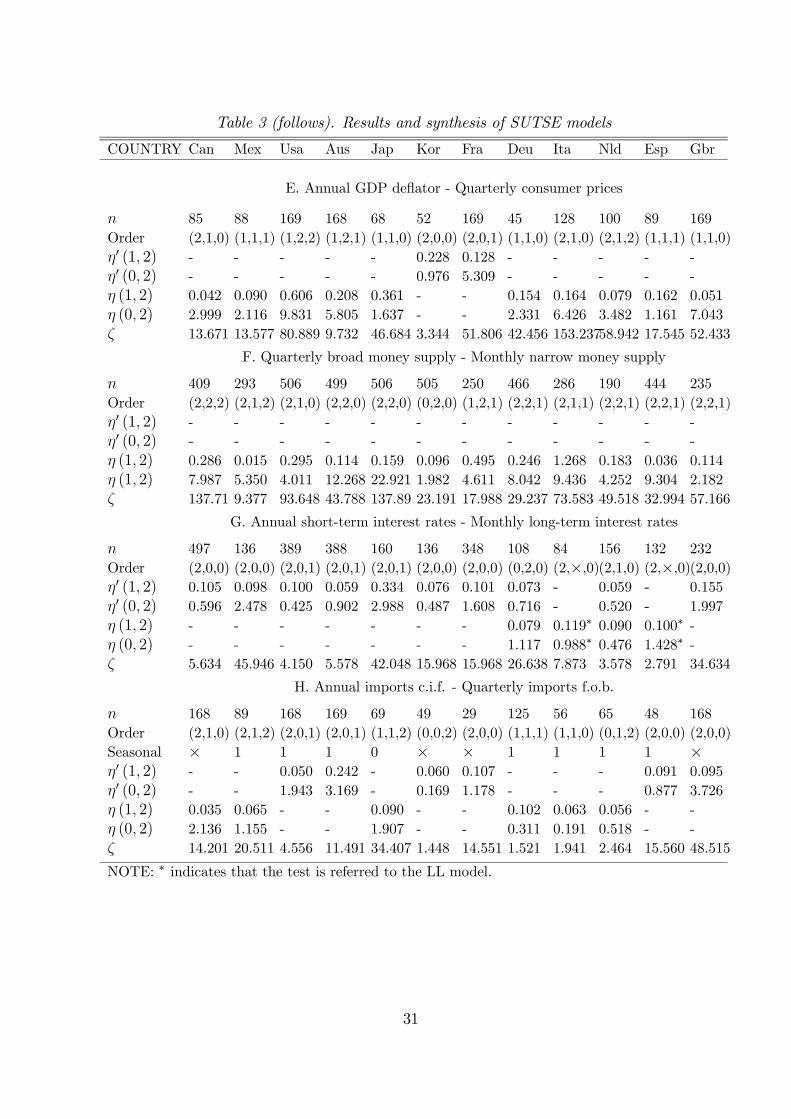
Table 3 (follows). Results and synthesis of SUTSE models


E. Annual GDP deflator - Quarterly consumer prices

n 85 88 169 168 68 52 169 45 128 100 89 169Order (2,1,0) (1,1,1) (1,2,2) (1,2,1) (1,1,0) (2,0,0) (2,0,1) (1,1,0) (2,1,0) (2,1,2) (1,1,1) (1,1,0)η0 (1, 2) - - - - - 0.228 0.128 - - - - -η0 (0, 2) - - - - - 0.976 5.309 - - - - -η (1, 2) 0.042 0.090 0.606 0.208 0.361 - - 0.154 0.164 0.079 0.162 0.051η (0, 2) 2.999 2.116 9.831 5.805 1.637 - - 2.331 6.426 3.482 1.161 7.043ζ 13.671 13.577 80.889 9.732 46.684 3.344 51.806 42.456 153.23758.942 17.545 52.433

F. Quarterly broad money supply - Monthly narrow money supply

n 409 293 506 499 506 505 250 466 286 190 444 235Order (2,2,2) (2,1,2) (2,1,0) (2,2,0) (2,2,0) (0,2,0) (1,2,1) (2,2,1) (2,1,1) (2,2,1) (2,2,1) (2,2,1)η0 (1, 2) - - - - - - - - - - - -η0 (0, 2) - - - - - - - - - - - -η (1, 2) 0.286 0.015 0.295 0.114 0.159 0.096 0.495 0.246 1.268 0.183 0.036 0.114η (1, 2) 7.987 5.350 4.011 12.268 22.921 1.982 4.611 8.042 9.436 4.252 9.304 2.182ζ 137.71 9.377 93.648 43.788 137.89 23.191 17.988 29.237 73.583 49.518 32.994 57.166

G. Annual short-term interest rates - Monthly long-term interest rates

n 497 136 389 388 160 136 348 108 84 156 132 232Order (2,0,0) (2,0,0) (2,0,1) (2,0,1) (2,0,1) (2,0,0) (2,0,0) (0,2,0) (2,×,0)(2,1,0) (2,×,0)(2,0,0)η0 (1, 2) 0.105 0.098 0.100 0.059 0.334 0.076 0.101 0.073 - 0.059 - 0.155η0 (0, 2) 0.596 2.478 0.425 0.902 2.988 0.487 1.608 0.716 - 0.520 - 1.997η (1, 2) - - - - - - - 0.079 0.119∗ 0.090 0.100∗ -η (0, 2) - - - - - - - 1.117 0.988∗ 0.476 1.428∗ -ζ 5.634 45.946 4.150 5.578 42.048 15.968 15.968 26.638 7.873 3.578 2.791 34.634

H. Annual imports c.i.f. - Quarterly imports f.o.b.

n 168 89 168 169 69 49 29 125 56 65 48 168Order (2,1,0) (2,1,2) (2,0,1) (2,0,1) (1,1,2) (0,0,2) (2,0,0) (1,1,1) (1,1,0) (0,1,2) (2,0,0) (2,0,0)Seasonal × 1 1 1 0 × × 1 1 1 1 ×η0 (1, 2) - - 0.050 0.242 - 0.060 0.107 - - - 0.091 0.095η0 (0, 2) - - 1.943 3.169 - 0.169 1.178 - - - 0.877 3.726η (1, 2) 0.035 0.065 - - 0.090 - - 0.102 0.063 0.056 - -η (0, 2) 2.136 1.155 - - 1.907 - - 0.311 0.191 0.518 - -ζ 14.201 20.511 4.556 11.491 34.407 1.448 14.551 1.521 1.941 2.464 15.560 48.515

NOTE: ∗ indicates that the test is referred to the LL model.

31

temporal disaggregation using multivariate structural … of structural time series models (see,...

Documents