Temporal data

• Stock market data

• Robot sensors

• Weather data

• Biological data: e.g. monitoring fish population.

• Network monitoring

• Weblog data

• Customer transactions

• Clinical data

• EKG and EEG data

• Industrial plan monitoring

Temporal data have a unique structure:

High dimensionality

High feature correlation

Requires special data mining techniques

Iyad Batal

Temporal data

• Sequential data (no explicit time) vs. time series data

– Sequential data e.g. : Gene sequences (we care about the order,

but there is no explicit time!).

• Real valued series vs. symbolic series

– Symbolic series e.g.: customer transaction logs.

• Regularly sampled vs irregularly sampled time series

– Regularly sampled time series e.g.: stock data.

– Irregularly sampled time series e.g.: weblog data, disc accesses.

• Univariate vs multivariate

– Mulitvarite time series e.g.: EEG data

Example: clinical datasets are usually multivariate, real valued and

irregularly sampled time series.Iyad Batal

0 50 0 1000 150 0 2000 2500

0 20 40 60 80 100 120 140 0 20 40 60 80 100 120 140 0 20 40 60 80 100 120 140

A B C

A B C

Classification

Query by ContentRule Discovery

sup = 0.5

conf= 0.6

Motif Discovery

Anomaly Detection

Clustering

Visualization

Temporal Data Mining Tasks

10

Iyad Batal

Temporal Data Mining

• Hidden Markov Model (HMM)

• Spectral time series representation

– Discrete Fourier Transform (DFT)

– Discrete Wavelet Transform (DWT)

• Pattern mining

– Sequential pattern mining

– Temporal abstraction pattern mining

Iyad Batal

Markov Models

• Set of states:

• Process moves from one state to another generating a

sequence of states:

• Markov chain property: probability of each subsequent state

depends only on what was the previous state:

• Markov model parameter

o transition probabilities:

o initial probabilities: )( ii sP

)|(),,,|( 1121 ikikikiiik ssPssssP

,,,, 21 ikii sss

},,,{ 21 Nsss

)|( jiij ssPa

Dry DryRain Rain Dry

Iyad Batal

Rain Dry

0.70.3

0.2 0.8

• Two states : Rain and Dry.

• Transition probabilities: P(Rain|Rain)=0.3 , P(Dry|Rain)=0.7 ,

P(Rain|Dry)=0.2, P(Dry|Dry)=0.8

• Initial probabilities: say P(Rain)=0.4 , P(Dry)=0.6.

• P({Dry, Dry, Rain, Rain} ) =

P(Dry) P(Dry|Dry) P(Rain|Dry) P(Rain|Rain)

= 0.6 * 0.8 * 0.2 * 0.3

Markov Model

Iyad Batal

• States are not visible, but each state randomly generates one of M

observations (or visible states)

• Markov model parameter: M=(A, B, )

o Transition probabilities:

o Initial probabilities:

o Emission probabilities:

Hidden Markov Model (HMM)

)|( jiij ssPa

)( ii sP

)|()( immi svPvb

High HighLow Low Low

Dry DryRain Rain Dry

Iyad Batal

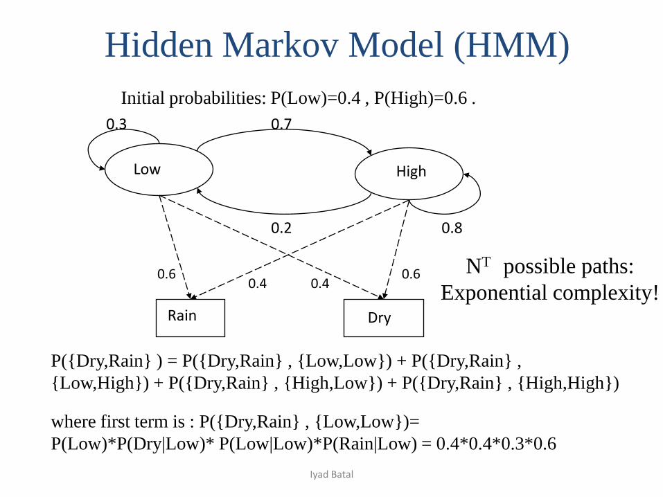
Hidden Markov Model (HMM)

P({Dry,Rain} ) = P({Dry,Rain} , {Low,Low}) + P({Dry,Rain} ,

{Low,High}) + P({Dry,Rain} , {High,Low}) + P({Dry,Rain} , {High,High})

where first term is : P({Dry,Rain} , {Low,Low})=

P(Low)*P(Dry|Low)* P(Low|Low)*P(Rain|Low) = 0.4*0.4*0.3*0.6

Low High

0.70.3

0.2 0.8

DryRain

0.6 0.60.4 0.4

Initial probabilities: P(Low)=0.4 , P(High)=0.6 .

NT possible paths:

Exponential complexity!

Iyad Batal

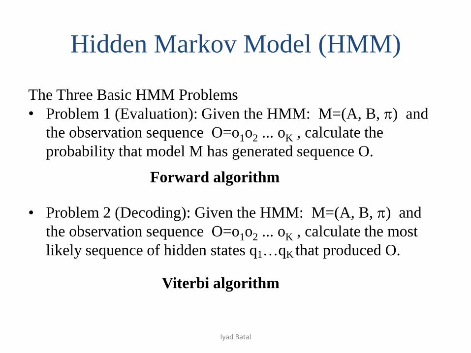
Hidden Markov Model (HMM)

The Three Basic HMM Problems

• Problem 1 (Evaluation): Given the HMM: M=(A, B, ) and

the observation sequence O=o1o2 ... oK , calculate the

probability that model M has generated sequence O.

• Problem 2 (Decoding): Given the HMM: M=(A, B, ) and

the observation sequence O=o1o2 ... oK , calculate the most

likely sequence of hidden states q1…qK that produced O.

Forward algorithm

Viterbi algorithm

Iyad Batal

Hidden Markov Model (HMM)

The Three Basic HMM Problems

• Problem 3 (Learning): Given some training observation

sequences O and general structure of HMM (numbers of

hidden and visible states), determine HMM parameters M=(A,

B, ) that best fit the training data, that is maximizes P(O|M).

Baum-Welch algorithm (EM)

Iyad Batal

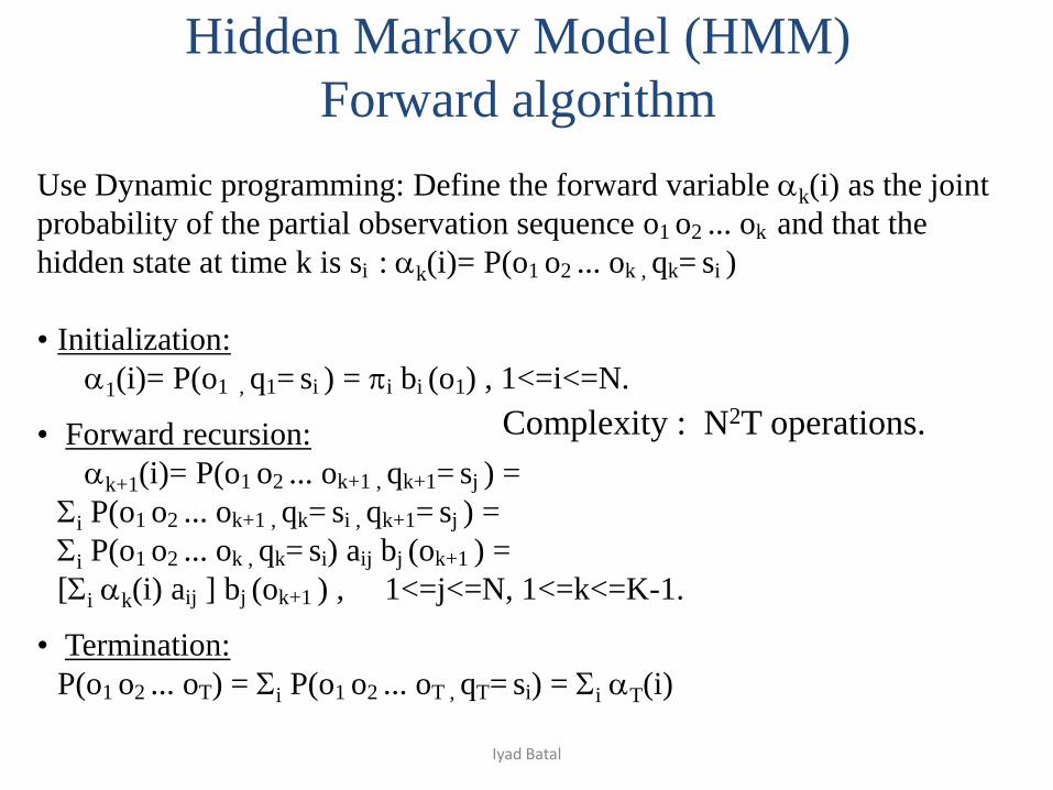
Use Dynamic programming: Define the forward variable k(i) as the joint

probability of the partial observation sequence o1 o2 ... ok and that the

hidden state at time k is si : k(i)= P(o1 o2 ... ok , qk= si )

• Initialization:

1(i)= P(o1 , q1= si ) = i bi (o1) , 1<=i<=N.

• Forward recursion:

k+1(i)= P(o1 o2 ... ok+1 , qk+1= sj ) =

i P(o1 o2 ... ok+1 , qk= si , qk+1= sj ) =

i P(o1 o2 ... ok , qk= si) aij bj (ok+1 ) =

[i k(i) aij ] bj (ok+1 ) , 1<=j<=N, 1<=k<=K-1.

• Termination:

P(o1 o2 ... oT) = i P(o1 o2 ... oT , qT= si) = i T(i)

Hidden Markov Model (HMM)

Forward algorithm

Complexity : N2T operations.

Iyad Batal

If training data has information about sequence of hidden states,

then use maximum likelihood estimation of parameters:

bi(vm ) = P(vm | si) =Number of times observation vm occurs in state si

Number of times in state si

Number of transitions from state sj to state si

Number of transitions out of state sj

aij= P(si | sj) =

i = P(si) = Number of times state Si occur at time k=1.

Hidden Markov Model (HMM)Baum-Welch algorithm

Iyad Batal

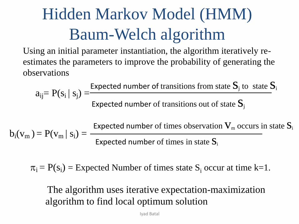
Using an initial parameter instantiation, the algorithm iteratively re-

estimates the parameters to improve the probability of generating the

observations

bi(vm ) = P(vm | si) =Expected number of times observation vm occurs in state si

Expected number of times in state si

Hidden Markov Model (HMM)

Baum-Welch algorithm

Expected number of transitions from state sj to state si

Expected number of transitions out of state sj

aij= P(si | sj) =

i = P(si) = Expected Number of times state Si occur at time k=1.

The algorithm uses iterative expectation-maximization

algorithm to find local optimum solutionIyad Batal

Temporal Data Mining

• Hidden Markov Model (HMM)

• Spectral time series representation

– Discrete Fourier Transform (DFT)

– Discrete Wavelet Transform (DWT)

• Pattern mining

– Sequential pattern mining

– Temporal abstraction pattern mining

Iyad Batal

DFT

• Discrete Fourier transform (DFT) transforms the series from the

time domain to the frequency domain.

• Given a sequence x of length n, DFT produces n complex numbers:

Remember that exp(jϕ)=cos(ϕ) + j sin(ϕ).

• DFT coefficients (Xf) are complex numbers: Im(Xf) is sine at

frequency f and Re(Xf) is cosine at frequency f, but X0 is always a

real number.

• DFT decomposes the signal into sine and cosine functions of several

frequencies.

• The signal can be recovered exactly by the inverse DFT:Iyad Batal

DFT

• DFT can be written as a matrix operation where A is a n x n matrix:

A is column-orthonormal.

Geometric view: view series x as a point in n-dimensional space.

• A does a rotation (but no scaling) on the vector x in n-dimensional

complex space:

– Does not affect the length

– Does not affect the Euclidean distance between any pair of

points

Iyad Batal

DFT

• Symmetry property: Xf=(Xn-f)* where * is the complex conjugate, therefore, we keep only the first half of the spectrum.

• Usually, we are interested in the amplitude spectrum (|Xf|) of the signal:

• The amplitude spectrum is insensitive to shifts in the time domain

• Computation:

– Naïve: O(n2)

– FFT: O(n log n)

Iyad Batal

DFT

Example1:

Very good compression!

We show only half the spectrum because of the symmetry

Iyad Batal

DFT

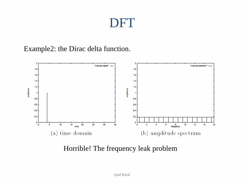
Example2: the Dirac delta function.

Horrible! The frequency leak problem

Iyad Batal

SWFT

• DFT assumes the signal to be periodic and have no temporal locality: each coefficient provides information about all time points.

• Partial remedy: the Short Window Fourier Transform (SWFT) divides the time sequence into non-overlapping windows of size w and perform DFT on each window.

• The delta function have restricted ‘frequency leak’.

• How to choose the width w?

– Long w gives good frequency resolution and poor time resolution.

– Short w gives good time resolution and poor frequency resolution.

• Solution: let w be variable → Discrete Wavelet Transform (DWT)

Iyad Batal

DWT

• DWT maps the signal into a joint time-frequency domain.

• DWT hierarchically decomposes the signal using windows of different

sizes (multi resolution analysis):

– Good time resolution and poor frequency resolution at high frequencies.

– Good frequency resolution and poor time resolution at low frequencies.

Iyad Batal

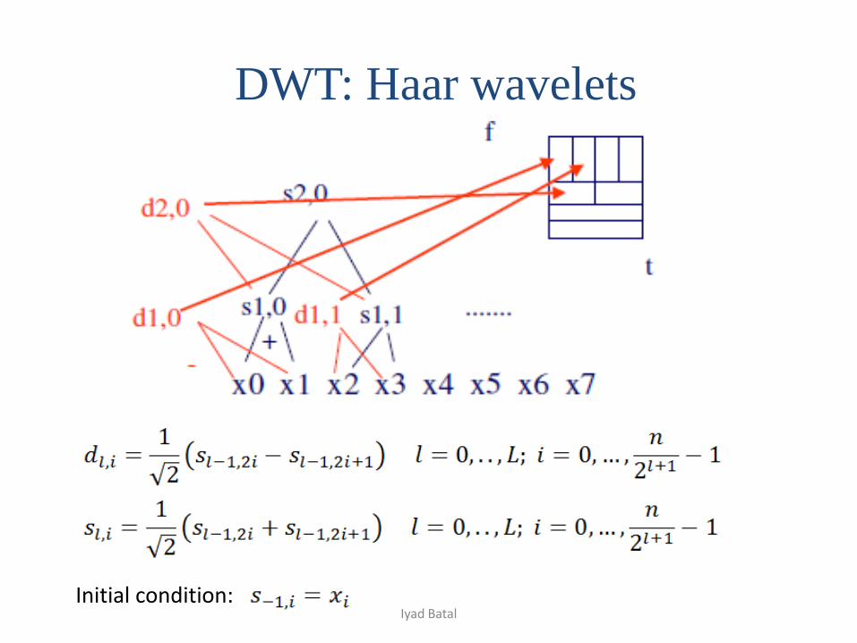
DWT: Haar wavelets

Initial condition:Iyad Batal

DWT: Haar wavelets

Length of the series should be a power of 2: zero pad the series!

Computational complexity is O(n)

The Haar transform: all the difference values dl,i at every level l and

offset i (n-1) difference, plus the smooth component sL,0 at the last level

Iyad Batal

DFT and DWT

• Both DFT and DWT are orthonormal transformations → rotation in

the space → do not affect the length or the Euclidean distance

between the series → clustering or classification in the transformed

space will give the exact same result!

• DFT/DWT are very useful for dimensionality reduction: usually a

small number of low frequency coefficients can approximate well

most time series/images.

• DFT/DWT are very useful for query by content using the GEMINI

framework:

– A quick and dirty filter (some false alarms, but no false dismissal).

– A spatial index (e.g R-tree) using few DFT or DWT coefficients.

Iyad Batal

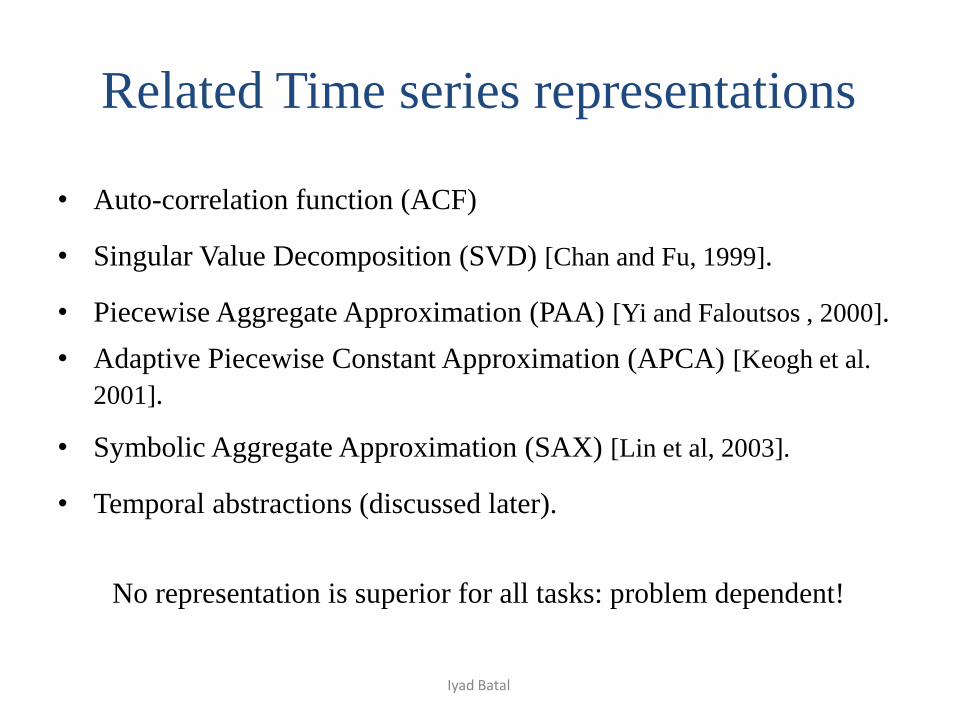
Related Time series representations

• Auto-correlation function (ACF)

• Singular Value Decomposition (SVD) [Chan and Fu, 1999].

• Piecewise Aggregate Approximation (PAA) [Yi and Faloutsos , 2000].

• Adaptive Piecewise Constant Approximation (APCA) [Keogh et al.

2001].

• Symbolic Aggregate Approximation (SAX) [Lin et al, 2003].

• Temporal abstractions (discussed later).

No representation is superior for all tasks: problem dependent!

Iyad Batal

Temporal Data Mining

• Hidden Markov Model (HMM)

• Spectral time series representation

– Discrete Fourier Transform (DFT)

– Discrete Wavelet Transform (DWT)

• Pattern mining

– Sequential pattern mining

– Temporal abstraction pattern mining

Iyad Batal

Sequential pattern mining

• A sequence is an ordered list of events, denoted < e1 e2 … eL >.

• Each event ei is an unordered set of items.

• Given two sequences α=< a1 a2 … an > and β=< b1 b2 … bm >

α is called a subsequence of β, denoted as α⊆ β, if there exist

integers 1≤ j1 < j2 <…< jn ≤m such that a1 ⊆ bj1, a2 ⊆ bj2,…, an ⊆ bjn

– Example: <a(bc)dc> is a subsequence of <a(abc)(ac)d(cf)>

• If a sequence contains l items, we call it a l-sequence

– Example: <a(bc)dc> is a 5-sequence.

• The support of a sequence α is the number of data sequences that

contain α.

Iyad Batal

Sequential pattern mining

• Given a set of sequences and support threshold, find the complete

set of frequent subsequences, from which we extract temporal rules.

– Examples: customers who buy a Canon digital camera are likely

to buy an HP color printer within a month.

A sequence database

SID sequence

1 <a(abc)(ac)d(cf)>

2 <(ad)c(bc)(ae)>

3 <(ef)(ab)(df)cb>

4 <eg(af)cbc>

Given support threshold min_sup =2,

<(ab)c> is a sequential pattern (s is

contained in sequences 1 and 3)

Iyad Batal

Sequential pattern mining

The GSP algorithm

GSP (Generalized Sequential Patterns: [Srikant & Agrawal 96]) is a generalization of Apriori for sequence databases.

Apriori property: If a sequence S is not frequent, then none of the super-sequences of S are not frequent.

– E.g, <hb> is infrequent so are <hab> and <(ah)b>

• Outline of the method

– Initially, get all frequent 1-sequences

– for each level (i.e., sequences of length-k) do

• generate candidate length-(k+1) sequences from length-k frequent sequences

• scan database to collect support count for each candidate sequence

– repeat until no frequent sequence or no candidate can be found

Iyad Batal

Finding Length-1 Sequential Patterns

• Initial candidates:

– <a>, <b>, <c>, <d>, <e>, <f>, <g>, <h>

• Scan database once, count support for candidates

<a(bd)bcb(ade)>50

<(be)(ce)d>40

<(ah)(bf)abf>30

<(bf)(ce)b(fg)>20

<(bd)cb(ac)>10

SequenceSeq. ID

min_sup =2

Cand Sup

<a> 3

<b> 5

<c> 4

<d> 3

<e> 3

<f> 2

<g> 1

<h> 1

Sequential pattern miningThe GSP algorithm

Iyad Batal

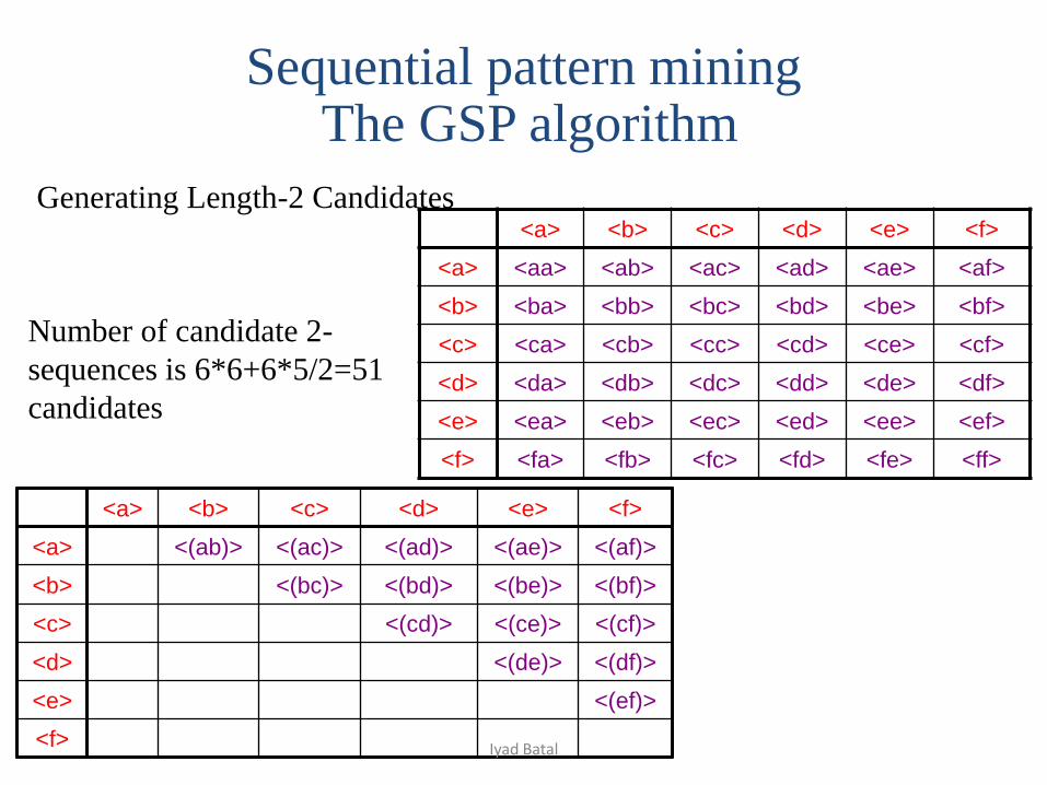
Generating Length-2 Candidates<a> <b> <c> <d> <e> <f>

<a> <aa> <ab> <ac> <ad> <ae> <af>

<b> <ba> <bb> <bc> <bd> <be> <bf>

<c> <ca> <cb> <cc> <cd> <ce> <cf>

<d> <da> <db> <dc> <dd> <de> <df>

<e> <ea> <eb> <ec> <ed> <ee> <ef>

<f> <fa> <fb> <fc> <fd> <fe> <ff>

<a> <b> <c> <d> <e> <f>

<a> <(ab)> <(ac)> <(ad)> <(ae)> <(af)>

<b> <(bc)> <(bd)> <(be)> <(bf)>

<c> <(cd)> <(ce)> <(cf)>

<d> <(de)> <(df)>

<e> <(ef)>

<f>

Number of candidate 2-

sequences is 6*6+6*5/2=51

candidates

Sequential pattern miningThe GSP algorithm

Iyad Batal

Candidate generation:

• Example1: join a and b:

– Sequential pattern mining: ab, ba, (ab)

– Itemset pattern mining: ab

• Example 2: join ab and ac:

– Sequential pattern mining: abc, acb, a(bc)

– Itemset pattern mining: abc

The number of candidates is much larger for sequential pattern mining!

Sequential pattern miningThe GSP algorithm

Iyad Batal

<a> <b> <c> <d> <e> <f> <g> <h>

<aa> <ab> … <af> <ba> <bb> … <ff> <(ab)> … <(ef)>

<abb> <aab> <aba> <baa> <bab> …

<abba> <(bd)bc> …

<(bd)cba>

1st scan: 8 cand. 6 length-1 seq. pat.

2nd scan: 51 cand. 19 length-2 seq. pat.

3rd scan: 46 cand. 19 length-3 seq. pat.

4th scan: 8 cand. 6 length-4 seq. pat.

5th scan: 1 cand. 1 length-5 seq. pat.

Cand. cannot pass sup. threshold

Cand. not in DB at all

<a(bd)bcb(ade)>50

<(be)(ce)d>40

<(ah)(bf)abf>30

<(bf)(ce)b(fg)>20

<(bd)cb(ac)>10

SequenceSeq. ID

min_sup =2

Sequential pattern mining

The GSP algorithm

Iyad Batal

Sequential pattern mining

Other sequential pattern mining algorithms:

• SPADE

– An Apriori-based and vertical data format algorithm.

• PrefixSpan

– Does not require candidate generation (similar to FP-growth).

• CloSpan:

– Mining Closed Sequential Patterns.

• Constraint based sequential pattern mining

Iyad Batal

Temporal abstraction

• Most of the time series representation techniques assume regularly

sampled univariate time series data.

• Many real-world temporal datasets (e.g. clinical data) are:

– Multivariate

– Irregularly sampled in time

• It is very difficult to directly model this type of data.

• We want to apply methods like sequential pattern mining, but on

multivariate time series data.

• Solution: use an abstract (qualitative) description of the series.

Iyad Batal

• Temporal abstraction moves from a time-point to an interval-based

representation in a way similar to humans’ perception of time series.

• Temporal abstraction converts (multivariate) time series T to state

sequences S: {(s1, b1, e1), (s2, b2, e2),…, (sn, bn, en)} where si denotes

an abstract state, bi < ei and bi <= bi+1.

• Abstract states usually defines primitive shapes in the data, e.g.:

– Trend abstractions: describe the series in terms of it local trends:

{increasing, steady, decreasing}

– Value abstractions: {high, normal, low}.

• These states are later combined to form more complex temporal

patterns.

Temporal abstraction

Iyad Batal

Temporal abstraction

Iyad Batal

A before B B after A

A equals B B equals A

A meets B A is-met-by B

A overlaps B A is-overlapped-by B

A during B B contains A

A starts B B is-started-by A

A finishes B B is-finished-by A

ABAB

AB

AB

ABABAB

Allen’s 13 temporal relations:

Maybe too specific for some applications: can be simplified to

fewer relations

Temporal relations

Iyad Batal

Temporal abstraction patterns

• Combine the abstract states using temporal relations to form

complex temporal patterns.

• Temporal pattern can be defined as a sequence of states

(intervals) related using temporal relationships.

– Example: P=low[X] before high[Y]

• These temporal patterns can be:

– User defined [Lucia et al. 2005]

– Automatically discovered [Hoppner 2001, Batal et al

2009].

Iyad Batal

Temporal abstraction patterns mining

(sketch)

• Sliding window option: interesting patterns can be limited in their

temporal extensions.

• More complicated (larger search space) than sequential pattern

mining because we have many temporal relations.

• We got Frequent temporal patterns, so what?

– Extract temporal rules

o inc[x] overlaps dec[y] ⇒ low[z]: sup=10%, conf=70%.

o knowledge discovery or prediction

– Use discriminative temporal patterns for classification

– Use temporal patterns to define clusters

– …

Iyad Batal