temporal correlation patterns in pre-seismic...

Physics and Chemistry of the Earth xxx (2015) xxx–xxx

Contents lists available at ScienceDirect

Physics and Chemistry of the Earth

journal homepage: www.elsevier .com/locate /pce

Temporal correlation patterns in pre-seismic electromagnetic emissionsreveal distinct complexity profiles prior to major earthquakes

http://dx.doi.org/10.1016/j.pce.2015.03.0081474-7065/� 2015 Elsevier Ltd. All rights reserved.

⇑ Corresponding author. Tel.: +49 331 288 2064; fax: +49 331 288 2640.E-mail addresses: [email protected] (R.V. Donner), [email protected] (S.

M. Potirakis), [email protected] (G. Balasis), [email protected] (K. Eftaxias), [email protected] (J. Kurths).

Please cite this article in press as: Donner, R.V., et al. Temporal correlation patterns in pre-seismic electromagnetic emissions reveal distinct comprofiles prior to major earthquakes. J. Phys. Chem. Earth (2015), http://dx.doi.org/10.1016/j.pce.2015.03.008

Reik V. Donner a,⇑, Stelios M. Potirakis b, Georgios Balasis c, Konstantinos Eftaxias d, Jürgen Kurths a,e,f,g

a Research Domain IV – Transdisciplinary Concepts and Methods, Potsdam Institute for Climate Impact Research, Telegrafenberg A31, 14473 Potsdam, Germanyb Department of Electronics Engineering, Piraeus University of Applied Sciences, 250 Thivon & P. Ralli, 12244 Aigaleo, Athens, Greecec Institute for Astronomy, Astrophysics, Space Applications and Remote Sensing, National Observatory of Athens, Metaxa and Vasileos Pavlou, Penteli, 15236 Athens, Greeced Section of Solid State Physics, Department of Physics, University of Athens, Panepistimiopolis, Zografos, 15784 Athens, Greecee Department of Physics, Humboldt University, Newtonstraße 15, 12489 Berlin, Germanyf Institute for Complex Systems and Mathematical Biology, University of Aberdeen, Aberdeen AB243UE, United Kingdomg Department of Control Theory, Nizhny Novgorod State University, Gagarin Avenue 23, 606950 Nizhny Novgorod, Russia

a r t i c l e i n f o

Article history:Received 5 November 2014Received in revised form 1 March 2015Accepted 23 March 2015Available online xxxx

Keywords:Pre-seismic electromagnetic emissionsEarthquake preparation processesCorrelationsDynamical complexity

a b s t r a c t

In the last years, continuous recordings of electromagnetic emissions from geophysical observatorieshave been recognized to exhibit characteristic fluctuation patterns prior to some major earthquakes.To further evaluate and quantify these findings, this work presents a detailed assessment of the time-varying correlation properties of such emissions during the preparatory phases preceding some recentearthquakes in Greece and Italy. During certain stages before the earthquakes’ occurrences, the electro-magnetic variability profiles are characterized by a marked increase in the degree of organization offluctuations, which allow developing hypotheses about the underlying physical mechanisms. Based onthe preparatory phases of selected seismic events, the information provided by different statistical prop-erties characterizing complementary aspects of the time-varying complexity based on temporal correla-tions is systematically assessed. The obtained results allow further insights into different pre-seismicstages based on the variability of electromagnetic emissions, which are probably associated with distinctgeophysical processes.

� 2015 Elsevier Ltd. All rights reserved.

1. Introduction

Earthquakes (EQ) are large-scale fracture phenomena arising inthe Earth’s heterogeneous crust, the occurrence of which is per-ceived in the form of a sudden violent shaking of the Earth’s sur-face. However, the processes involved in the preparation of anEQ are complex and not easy to be directly monitored. Therefore,the view that ‘‘understanding how earthquakes occur is one ofthe most challenging questions in fault and earthquake mechanics’’(Shimamoto and Togo, 2012) is not an overstatement. In the direc-tion of understanding the underlying complex nonlinear processesinvolved in the preparation of an EQ, two research fields haveattracted the particular interest of scientists. One of them, to whichhuge efforts have been devoted, is the study of fracture phenomenaat the laboratory scale (e.g., Lockner et al., 1991; Lockner, 1996;Chauhan and Misra, 2008; Johnson et al., 2008; Baddari and

Frolov, 2010; Ben-David et al., 2010; Zapperi, 2010; Baddariet al., 2011; Lacidogna et al., 2011; Hadjicontis et al., 2011;Schiavi et al., 2011; Carpinteri et al., 2012; Chang et al., 2012),while the other is the study of different phenomena which areobserved in the field prior to the occurrence of significant EQs.

It has been shown that opening cracks are accompanied withelectro-magnetic emissions (EME) covering a wide frequency spec-trum from the kHz band to the MHz band. These signals can befound at the laboratory scale prior to global failure in fractureexperiments (e.g., Chauhan and Misra, 2008; Baddari et al., 2011;Lacidogna et al., 2011; Hadjicontis et al., 2011; Carpinteri et al.,2012), as well as at the geophysical scale prior to significant EQs(e.g., Warwick et al., 1982; Hayakawa and Fujinawa, 1994; Qianet al., 1994; Gokhberg et al., 1995; Kapiris et al., 2004;Contoyiannis et al., 2005, 2015; Uyeda et al., 2009; Ciceroneet al., 2009; Potirakis et al., 2012, 2013, 2015; Eftaxias et al.,2013; Eftaxias and Potirakis, 2013). Two important features ofEME have been observed in both the laboratory and the field: (i)emissions in the MHz band consistently precede those in the kHzband, indicating that each type of those emissions corresponds todifferent characteristic stages of the fracture/EQ preparation, while

plexity

http://dx.doi.org/10.1016/j.pce.2015.03.008

mailto:[email protected]







http://www.sciencedirect.com/science/journal/14747065

http://www.elsevier.com/locate/pce


2 R.V. Donner et al. / Physics and Chemistry of the Earth xxx (2015) xxx–xxx

(ii) after the emission of the kHz EME an electro-magnetic quies-cence systematically emerges before the time of the global fail-ure/EQ occurrence (Kumar and Misra, 2007; Qian et al., 1994;Baddari and Frolov, 2010; Hayakawa and Fujinawa, 1994;Gokhberg et al., 1995; Matsumoto et al., 1998; Hayakawa, 1999;Eftaxias et al., 2013; Eftaxias and Potirakis, 2013; and referencestherein). Based on these features and the results obtained throughthe analysis of field observations of MHz-kHz EME by multidisci-plinary time-series analysis tools, the following four-stage modelof the EQ preparation process by means of fracture-induced EMEhas been proposed recently (Eftaxias and Potirakis, 2013, and refer-ences therein; Contoyiannis et al., 2015, and references therein):

(1) The initially emerging MHz EM field is attributed to crackingin the highly disordered material that surrounds the back-bone of strong entities (asperities) distributed around thestressed fault sustaining the system. It has been shown usingthe Method of Critical Fluctuations (MCF) that this emissionshows anti-persistency and can be described in analogy to athermal second-order phase transition in equilibrium(Contoyiannis et al., 2005, and references therein). Moredetailed analysis by means of truncated Lévy statistics andnon-extensive Tsallis statistical mechanics suggests that atruncated Lévy walk-type mechanism can organize the het-erogeneous system to criticality (Contoyiannis and Eftaxias,2008). Importantly, based on the recently introducedmethod of natural time analysis (Varotsos et al., 2011a, b),it has been shown that the seismic activity that occurs inthe region around the epicenter of the forthcoming signifi-cant shock a few days up to approximately one week beforethe main shock occurrence, as well as the observed MHz EMprecursor which emerges during the same period of time,both behave as critical phenomena (Potirakis et al., 2013,2015).

(2) Our understanding of different rupture modes is still verymuch in its infancy. However, laboratory experiments ofrock fracture and frictional sliding have shown that the rela-tive slip of two fault surfaces takes place in two phases: aslow stick–slip like fracture-sliding precedes dynamical fastglobal slip (Ben-David et al., 2010; Chang et al., 2012). It hasbeen suggested that the abrupt emergence of a strong ava-lanche-like kHz EM field is due to the fracture of the familyof the asperities themselves, namely to the slow stick–sliplike stage of the rupture mode. This emission exhibits a highinformation content and organization, a preferred directionin the underlying fracto-EM mechanism and persistency,i.e., it includes key features of an extreme event (Eftaxiaset al., 2013; Eftaxias and Potirakis, 2013; and referencestherein). The observed kHz EM precursor is characterizedby the absence of any footprint of a second-order transitionin equilibrium or a truncated Lévy walk-type mechanism.On the contrary, it shows footprints of a first-order phasetransition (Contoyiannis et al., 2015). The kHz EM time ser-ies includes well-established universal structural patterns offracture-faulting processes, namely: (i) the activation of asingle fault by means of kHz EM activity behaves as a redu-ced/magnified image of the regional/laboratory seismicity;(ii) its temporal profile is consistent with the universal frac-tional Brownian motion-type spatial profile of natural rocksurfaces; (iii) the roughness of its temporal profile coincideswith the universal spatial roughness of fracture surfaces.Finally, the kHz EM emission is consistent with the faultmodeling of the occurred earthquake, which is supportedby studies from different disciplines, e.g., satellite radarinterferometry and seismology (Eftaxias et al., 2013;Eftaxias and Potirakis, 2013; and references therein).

Please cite this article in press as: Donner, R.V., et al. Temporal correlation patprofiles prior to major earthquakes. J. Phys. Chem. Earth (2015), http://dx.doi.o

(3) Recently, it has been shown by means of the MCF that inbetween the above mentioned two stages of the fractureprocess, there exists an intermediate stage which reflectsthe tri-critical behavior (Contoyiannis et al., 2015). Thisstage appears in the kHz EME just before the emergence ofthe strong avalanche-like kHz emission. The results obtainedfor the kHz time series are compatible with those for anintroduced model map which describes the tri-critical cross-over. The tri-critical crossover indicates the boundary of ananti-persistent dynamics, namely the existence of a negativefeedback mechanism that kicks the system away fromextreme behavior.

(4) The systematically observed EM quiescence in all frequencybands is rooted in the stage of preparation of dynamical slip,which results in the fast, even super-shear, mode that sur-passes the shear wave speed. Recent laboratory experimentsalso reveal this feature.

In summary, the proposed four stages of the last part of EQ pre-paration process and the associated EM observables appear in thefollowing order: 1st stage: valid MHz anomaly; 2nd stage: kHzanomaly exhibiting tri-critical characteristics; 3rd stage: strongavalanche-like kHz anomaly; 4th stage: electromagneticquiescence.

We note that the study of EME possibly related with an upcom-ing significant seismic event is associated with the existence of‘‘paradox features’’ that accompany their observation, expressedin the form of the following research questions: Why is EM quies-cence observed at the time of the EQ occurrence? Why are theemerging EM signals not accompanied by large precursory strainchanges, much larger than co-seismic ones? Why are the EM emis-sions not observed during the aftershock period? How is the trace-ability of potential EM precursors achieved given that they shouldnormally be absorbed by the Earth’s crust? A first attempt toanswering these questions has been recently presented (Eftaxiaset al., 2013; Eftaxias and Potirakis, 2013; and references therein).

The above suggested four-stage model of EQ preparation pro-cesses by means of fracture-induced EME is a hypothesis thatremains to be further verified. However, it should be noted that,up to now, it seems to be in agreement with both experimental(laboratory and geophysical) data, as well as theoretic and sim-ulation studies of fracture phenomena, while no rebuttal has beenpublished yet.

In this work, we focus on the third stage and the analysis of thestrong avalanche-like kHz EME; all the herein analyzed signals arestrong avalanche-like kHz anomalies, corresponding to the samestage, the third stage, of our proposed four-stage model. Due tothe important practical implications of the hypothesis that theseemissions signify the fracture of asperities, which means that afterthe observation of valid recorded kHz signals the EQ occurrence isinevitable, it is crucial to apply further analysis methods whichhelp identifying those features embedded in the kHz EME thatcould possibly reveal the validity of such recordings. As it wasmentioned, a crucial footprint of an extreme event is its highdegree of organization. Such a feature should be included in afracto-EM activity rooted in the fracture of asperities. It is impor-tant to note that ‘‘there is no way to find an optimum organizationor complexity measure’’ (Kurths et al., 1995). Therefore, in thiswork we search for further evidence for the (temporary) existenceof a dynamical state of high organization, which clearly discrimi-nates an emerging kHz anomaly prior to a large EQ from the back-ground EM noise in the region of the recording station. For thispurpose, we utilize different measures characterizing the dynami-cal complexity of geophysical signals based on their linear correla-tion structure, an approach that has been originally proposed byDonner and Witt (2006, 2007) in a multivariate framework and

terns in pre-seismic electromagnetic emissions reveal distinct complexityrg/10.1016/j.pce.2015.03.008


R.V. Donner et al. / Physics and Chemistry of the Earth xxx (2015) xxx–xxx 3

recently been adopted for defining an easily calculable complexitymeasure for univariate time series (Donner and Balasis, 2013). Inthis work, we complement the previously developed analysis strat-egy by a suite of additional measures quantifying different aspectsassociated with the correlation structure of pre-seismic EME.

The remainder of this manuscript is organized as follows:Section 2 describes the EME data used in this study. The analysismethodology used in this work is detailed in Section 3.Subsequently, the results of our investigations are presented inSection 4 and put into the context of previous findings in Section 5.

2. Data

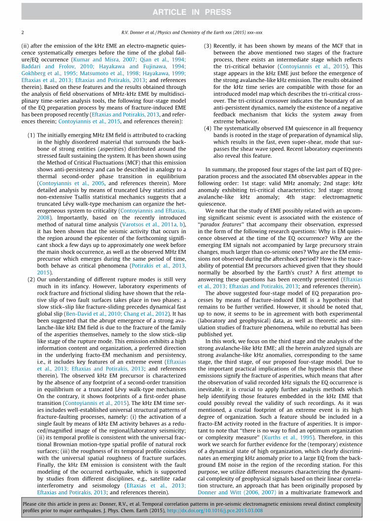
The kHz EME time series analyzed in the present work have allbeen recorded at the exemplary remote telemetric station atZakynthos (Zante) Island in the Ionian Sea (western Greece), usinginstrumentation developed by Nomicos (Nomikos et al., 1997).Zakynthos Island is located at a region of high tectonic activity,right on the Hellenic Arc (Kopanas, 1997), cf. Fig. 1. The telemetricstation has been installed on a carefully selected mountainous siteat the south-west of the island (37.76� N, 20.76� E) providing at thesame time very low background noise and high Earth conductivity(Antonopoulos, 1996; Makris et al., 1999; Eftaxias et al., 2001).These features render this specific station particularly appropriatefor magnetic field strength measurements, i.e. for kHz EME detec-tion. The kHz EME are measured by six loop antennas detecting thethree components, east–west (EW), north–south (NS), and vertical,of the variations of the magnetic field at 3 kHz and 10 kHz, respec-tively. The EME time series are sampled once per second, i.e., witha sampling frequency of 1 Hz. More information about the experi-mental setup can be found in the supplementary material ofPotirakis et al. (2015).

The analyzed kHz EME time series were detected prior to threesignificant EQs which happened in Greece and Italy, cf. Fig. 1. Inchronological order, these EQs are the Kozani-Grevena EQ [oc-curred on 13 May 1995 (08:47:13 UT) in northern Greece withan epicenter at 40.17� N, 21.68� E and a magnitude of 6.5] (e.g.,Kapiris et al., 2002, 2003; Eftaxias et al., 2002; Contoyianniset al., 2005), the Athens EQ [with magnitude 5.9, occurred on 7September 1999 (11:56:49 UT) in central Greece (38.15� N,

Fig. 1. Location of the recording station at Zakynthos a


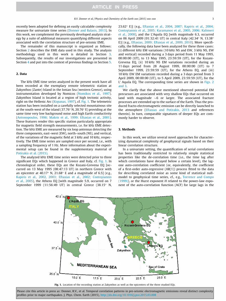
23.62� E)] (e.g., Eftaxias et al., 2004, 2007; Kapiris et al., 2004;Contoyiannis et al., 2005; Karamanos et al., 2005, 2006; Kalimeriet al., 2008), and the L’Aquila EQ [with magnitude 6.3, occurredon 06 April 2009 (01:32:41 UT) in central Italy (42.34� N, 13.38�E)] (e.g., Eftaxias, 2009; Eftaxias et al., 2009, 2010). More specifi-cally, the following data have been analyzed for these three cases:(i) different kHz EM variations (10 kHz NS and EW, 3 kHz NS, EWand vertical) recorded during a 3 days period from 11 May 1995,00:00:00 (UT), to 13 May 1995, 23:59:59 (UT), for the Kozani-Grevena EQ, (ii) 10 kHz NS EM variations recorded during an11 days period from 28 August 1999, 00:00:00 (UT) to 7September 1999, 23:59:59 (UT), for the Athens EQ, and (iii)10 kHz EW EM variations recorded during a 3 days period from 3April 2009, 00:00:00 (UT), to 5 April 2009, 23:59:59 (UT), for theL’ Aquila EQ. The corresponding time series are shown in Figs. 2and 3.

We clarify that the above mentioned observed potential EMprecursors are associated with very shallow EQs that occurred onland with magnitude �6 or larger. The associated fractureprocesses are extended up to the surface of the Earth. Thus the pro-duced fracto-electromagnetic emission can be directly launched tothe atmosphere (Eftaxias and Potirakis, 2013 and referencestherein). In turn, comparable signatures of deeper EQs are com-monly harder to observe.

3. Methods

In this work, we utilize several novel approaches for character-izing dynamical complexity of geophysical signals based on theirlinear correlation structure.

In a univariate setting, the quantification of serial correlationshas been traditionally restricted to relatively simple statisticalproperties like the de-correlation time (i.e., the time lag afterwhich correlations have decayed below a certain level), the lag-one auto-correlation coefficient (or, equivalently, the coefficientof a first-order auto-regressive (AR(1)) process fitted to the datafor describing correlated noise as some kind of statistical null-model to geophysical time series, cf., e.g., Torrence and Compo(1999)), or the Hurst exponent H related to the power-law expo-nent of the auto-correlation function (ACF) for large lags in the

s well as the epicenters of the three studied EQs.



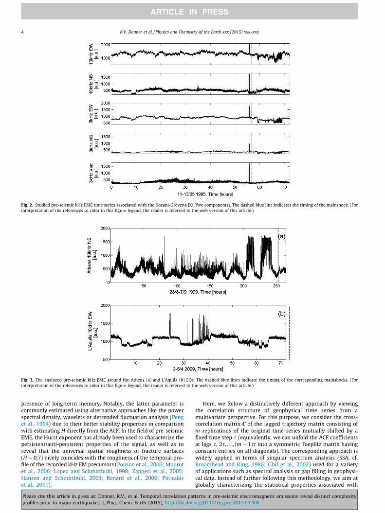
Fig. 2. Studied pre-seismic kHz EME time series associated with the Kozani-Grevena EQ (five components). The dashed blue line indicates the timing of the mainshock. (Forinterpretation of the references to color in this figure legend, the reader is referred to the web version of this article.)

Fig. 3. The analyzed pre-seismic kHz EME around the Athens (a) and L’Aquila (b) EQs. The dashed blue lines indicate the timing of the corresponding mainshocks. (Forinterpretation of the references to color in this figure legend, the reader is referred to the web version of this article.)


presence of long-term memory. Notably, the latter parameter iscommonly estimated using alternative approaches like the powerspectral density, wavelets or detrended fluctuation analysis (Penget al., 1994) due to their better stability properties in comparisonwith estimating H directly from the ACF. In the field of pre-seismicEME, the Hurst exponent has already been used to characterize thepersistent/anti-persistent properties of the signal, as well as toreveal that the universal spatial roughness of fracture surfaces(H � 0.7) nicely coincides with the roughness of the temporal pro-file of the recorded kHz EM precursors (Ponson et al., 2006; Mourotet al., 2006; Lopez and Schmittbuhl, 1998; Zapperi et al., 2005;Hansen and Schmittbuhl, 2003; Renard et al., 2006; Potirakiset al., 2011).


Here, we follow a distinctively different approach by viewingthe correlation structure of geophysical time series from amultivariate perspective. For this purpose, we consider the cross-correlation matrix C of the lagged trajectory matrix consisting ofm replications of the original time series mutually shifted by afixed time step s (equivalently, we can unfold the ACF coefficientsat lags s, 2s, . . ., (m � 1)s into a symmetric Toeplitz matrix havingconstant entries on all diagonals). The corresponding approach iswidely applied in terms of singular spectrum analysis (SSA, cf.Broomhead and King, 1986; Ghil et al., 2002) used for a varietyof applications such as spectral analysis or gap filling in geophysi-cal data. Instead of further following this methodology, we aim atglobally characterizing the statistical properties associated with




this (positive semi-definite) correlation matrix. For this purpose,we study the associated spectrum of non-negative real eigenvaluesof C. Specifically, we utilize different characteristics inspired byfindings for correlation matrices in various other fields like finan-cial markets (Plerou et al., 2002), neurophysiology (Müller et al.,2005) and spatio-temporal chaos (Zoldi and Greenside, 1997).

First, we study the largest eigenvalue r12, which can be inter-

preted as the fraction of variance of the m-dimensional embeddedsystem explained by its first principal component. The partic-ipation ratio of the associated eigenvector (a11, . . ., a1m) (Plerouet al., 2002; Müller et al., 2005)

p1 ¼ mXm

j¼1

ja1jj4 !�1

ð1Þ

characterizes how strong different lags contribute to this compo-nent. Due to the fourth power of the eigenvector coefficients, direc-tions in the embedding space (i.e., time lags) contributing stronglyto the first eigenvector receive much stronger weight than thosehaving minor relevance. Hence, if there are only a few relevant timelags, the sum will be large, so that p1 takes small values. In turn, incase of a more balanced distribution (i.e., more time lags contribut-ing significantly to the first principal component, pointing to a morecomplex signal), we may expect higher values of p1.

Second, we compute the normalized Shannon entropy of thefull spectrum of eigenvalues r1

2, . . .,rm2 of C as follows: The eigen-

values are first normalized to unit sum. Then, we take the decadallogarithms of the normalized eigenvalues. The relative frequenciespk of logarithmic normalized eigenvalues to fall into K bins(k = 1, . . .,K) of the same size are evaluated and used for estimatingthe associated normalized Shannon entropy

S ¼ 1logK

XK

k¼1

pklogpk: ð2Þ

High values of S indicate a broad variety of eigenvalues (i.e., fewdominating ‘‘modes’’), whereas smaller values correspond to situa-tions where the eigenvalue spectrum is more concentrated (i.e.,there are many different ‘‘variability patterns’’ associated with dif-ferent combinations of time lags, which have comparable rele-vance). Note that in order to assure quantitative comparability ofthe results for different data sets and/or time slices, the same bin-ning needs to be considered. The number of bins K is to be selectedsuch that each bin contains on average a statistically sufficientnumber of eigenvalues, i.e., needs to be properly chosen accordingto the value of m. To our best knowledge, the Shannon entropy ofthe eigenvalue spectrum of C has not yet been used elsewhere forthe purpose of characterizing the time-varying degree of dynami-cal complexity of geophysical or other time series and thus pre-sents a novel methodological aspect of the present work. Weemphasize that the eigenvalue entropy S is not to be confused withthe classical Shannon entropy of the underlying signal itself, sinceit quantifies distinctively different properties of the data understudy. Specifically, when evaluated in terms of block or per-mutation entropies, high values of the Shannon entropy commonlyindicate higher dynamical disorder pointing to possibly highercomplexity of the underlying signal. In turn, high values of theeigenvalue entropy indicate a broad range of eigenvalues, i.e., vari-ability modes contained in the correlation structure of the datatend to have different variances instead of similar ones, whichcould be interpreted as a signature of low complexity.

Finally, we study the scaling of residual SSA variances whenmore and more eigenvalues of C are considered. For this purpose,consider again the eigenvalues ri

2 normalized to unit sum. The dif-ference between 1 and the sum of the first p normalized eigenval-ues gives the residual fraction of variance not explained by the first


p principal components of C (in SSA language, the first p recon-structed components). It has been found numerically that in manycases, the residual variances show a roughly exponential decay.The typical scale parameter associated with this decay is calledthe linear variance decay (LVD) dimension density (Donner andWitt, 2006, 2007; Donner et al., 2008). This parameter is estimatedby means of linear regression up to a given maximum fraction ofexplained variance f = 0.9 (see Donner et al. (2008) for full detailson the estimation procedure). Considering the limiting cases offully uncorrelated and perfectly linearly correlated components, anormalized LVD dimension density d can be defined, which takesvalues of d = 0 for perfect correlations (i.e., a deterministic signalwith constant values or some linear trend) and d = 1 for vanishingserial correlations (i.e., white noise), respectively (Xie et al., 2011).While the original approach has been developed for multivariatetime series, its modification for univariate records has recentlyfound several applications (Toonen et al., 2012; Donner andBalasis, 2013).

We emphasize that the four statistical parameters r12, p1, S and

d characterize different aspects associated with the correlationstructure of the signal under study. Specifically, the latter twocan be interpreted as measures of disorder and complexity of thecorrelation structure. Motivated by recent proposals for combiningconceptually similar pairs of measures in some complexity-en-tropy plane (Martin et al., 2006; Rosso et al., 2007), we will mainlyfocus on d and S in order to distinguish time intervals with differ-ent dynamical regimes in the pre-seismic kHz EME.

4. Results

4.1. Auto-correlation functions

Since all measures used in this study are based on the tradi-tional Pearson correlation, it appears justified to start our analysisby inspecting the structure of the ACFs associated with the differ-ent kHz pre-seismic EME records. Notably, the behavior of the ACFcan reveal important information on typical time-scales of fluctua-tions contained in the signal. For our corresponding analysis, wefirst take the global picture by disregarding the possible distinctioninto different phases prior and even after the occurrence of themainshock.

From Fig. 4, we conclude that all considered records showmarked non-stationarity expressed in terms of a generally veryslow decay of the ACFs for all considered signals. This effect is tobe expected given the different levels of kHz EME amplitudes dur-ing different stages of the EQ preparation processes as well as itsimmediate aftermath (cf. Figs. 2 and 3), which dominate the ACFwhen evaluated at this global scale. In order to address the prob-lem of non-stationarity at the level of mean EME amplitudes (butnot the superimposed short-term fluctuations), all records weresubjected to a moving-average detrending regarding mean valuestaken over centered windows in time with a width of 30 min.After this pre-processing, the data actually exhibit a relatively fastdecay of serial correlations as expected for approximately station-ary time series.

Looking in somewhat more detail at the shape of the ACFs, wefind that the recordings for the L’Aquila and Athens EQs display asmooth decay without any pronounced oscillatory components.The corresponding behavior is distinctively different for theKozani-Grevena EQ, where the five different recorded kHz EMEcomponents exhibit somewhat different correlation patterns.Specifically, in three of the five components (10 kHz EW, 3 kHzEW and 3 kHz NS) the ACF appears modulated with a signal ofabout 265 s period, while the two other components (10 kHz NSand 3 kHz vertical) exhibit similar but much faster modulations



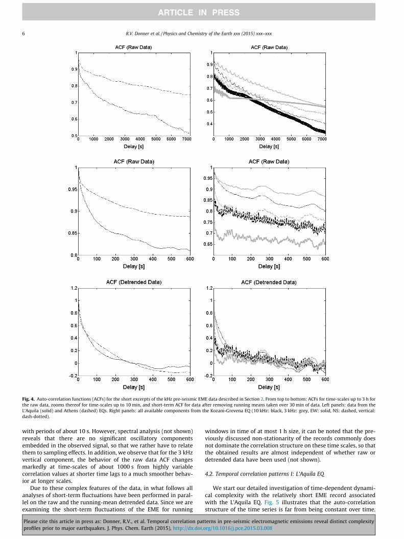
Fig. 4. Auto-correlation functions (ACFs) for the short excerpts of the kHz pre-seismic EME data described in Section 2. From top to bottom: ACFs for time-scales up to 3 h forthe raw data, zooms thereof for time-scales up to 10 min, and short-term ACF for data after removing running means taken over 30 min of data. Left panels: data from theL’Aquila (solid) and Athens (dashed) EQs. Right panels: all available components from the Kozani-Grevena EQ (10 kHz: black, 3 kHz: grey, EW: solid, NS: dashed, vertical:dash-dotted).


with periods of about 10 s. However, spectral analysis (not shown)reveals that there are no significant oscillatory componentsembedded in the observed signal, so that we rather have to relatethem to sampling effects. In addition, we observe that for the 3 kHzvertical component, the behavior of the raw data ACF changesmarkedly at time-scales of about 1000 s from highly variablecorrelation values at shorter time lags to a much smoother behav-ior at longer scales.

Due to these complex features of the data, in what follows allanalyses of short-term fluctuations have been performed in paral-lel on the raw and the running-mean detrended data. Since we areexamining the short-term fluctuations of the EME for running


windows in time of at most 1 h size, it can be noted that the pre-viously discussed non-stationarity of the records commonly doesnot dominate the correlation structure on these time scales, so thatthe obtained results are almost independent of whether raw ordetrended data have been used (not shown).

4.2. Temporal correlation patterns I: L’Aquila EQ

We start our detailed investigation of time-dependent dynami-cal complexity with the relatively short EME record associatedwith the L’Aquila EQ. Fig. 5 illustrates that the auto-correlationstructure of the time series is far from being constant over time.



Fig. 5. Time-dependent ACF (color-coded) up to a maximum lag of 5 min for running windows of 1 h and mutual offset of 1 min for the kHz EME record associated with theL’Aquila and Athens EQs. (For interpretation of the references to color in this figure legend, the reader is referred to the web version of this article.)


In contrast, we observe alternations between sequences of timewindows with very fastly and very slowly decaying ACF, suggest-ing qualitatively different physical processes causing thecorresponding emissions. Notably, a slow decay of correlations isa common manifestation of long-range dependences, whereas afast decay can often be observed in case of anti-persistentdynamics. We do not address the aspect of persistence here, sinceit is relatively hard to evaluate in the relatively short time windowsused here for a characterization of time-varying dynamical com-plexity. A more detailed corresponding study will be subject offuture work.

Based the observed complex temporal variability of auto-correlations, we proceed with calculating the different characteris-tics introduced in Section 3. The results of this investigation areshown in Figs. 6 and 7 for a window width of 1 h and mutual offsetof 1 min. Regarding the AR(1) coefficient, the largest eigenvalue r1

2

and its associated participation ratio p1 (Fig. 6), the observed vari-ability appears mutually consistent and mainly traces the afore-mentioned succession of time intervals with fast and slow ACFdecay, respectively. In turn, the eigenvalue entropy S and LVDdimension density d (Fig. 7) exhibit a more interesting patternprior to the EQ, although the complexity measure mainly co-varies

Fig. 6. Correlation-based characteristics for the L’Aquila EQ (computed for running windoassociated participation ratio p1.


with the AR(1) coefficient and the information associated with theleading eigenvalue. The latter behavior is to be expected, however,we emphasize that differences in the temporal profile of d fromthat of the other characteristics indicate a more complexdistribution of eigenvalues, deviating significantly from the pre-sumed exponential decay of residual variances underlying thismeasure.

Examining Fig. 7 in more detail, we find that there are timeintervals during which d drops to values close to 0, some of whichare in parallel characterized by a marked increase of S. The latterperiods can be found between about 23 and 41 h after the begin-ning of the record, while the EQ itself occurred at around 73.5 hand was unfortunately not covered by the available EME record.Intermittent to the aforementioned time interval, there are periodswith lower (but still gradually increasing) eigenvalue entropy andhigher (gradually decreasing) complexity. This intermittent behav-ior is obviously associated with pronounced spikes in the EME sig-nal, cf. Fig. 3b. Finally, the time interval between 41 h after the startof measurements and the EQ occurrence is characterized by (apartfrom an intermediate time window between about 52 and 60 h)high values of d, while S fluctuates around its relatively low base-line level. Notably, in contrast to d, S does not exhibit any further

ws of width 1 h, mutual offset of 1 min): AR(1) coefficient, largest eigenvalue r12 and



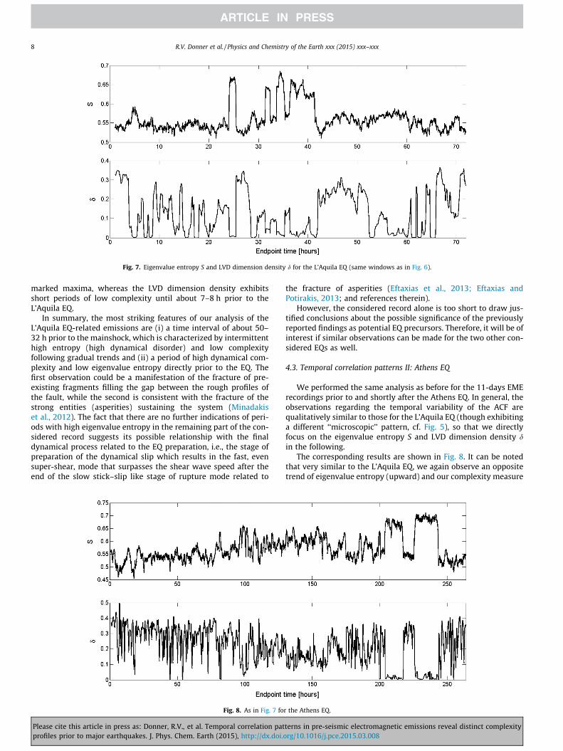
Fig. 7. Eigenvalue entropy S and LVD dimension density d for the L’Aquila EQ (same windows as in Fig. 6).


marked maxima, whereas the LVD dimension density exhibitsshort periods of low complexity until about 7–8 h prior to theL’Aquila EQ.

In summary, the most striking features of our analysis of theL’Aquila EQ-related emissions are (i) a time interval of about 50–32 h prior to the mainshock, which is characterized by intermittenthigh entropy (high dynamical disorder) and low complexityfollowing gradual trends and (ii) a period of high dynamical com-plexity and low eigenvalue entropy directly prior to the EQ. Thefirst observation could be a manifestation of the fracture of pre-existing fragments filling the gap between the rough profiles ofthe fault, while the second is consistent with the fracture of thestrong entities (asperities) sustaining the system (Minadakiset al., 2012). The fact that there are no further indications of peri-ods with high eigenvalue entropy in the remaining part of the con-sidered record suggests its possible relationship with the finaldynamical process related to the EQ preparation, i.e., the stage ofpreparation of the dynamical slip which results in the fast, evensuper-shear, mode that surpasses the shear wave speed after theend of the slow stick–slip like stage of rupture mode related to

Fig. 8. As in Fig. 7 fo


the fracture of asperities (Eftaxias et al., 2013; Eftaxias andPotirakis, 2013; and references therein).

However, the considered record alone is too short to draw jus-tified conclusions about the possible significance of the previouslyreported findings as potential EQ precursors. Therefore, it will be ofinterest if similar observations can be made for the two other con-sidered EQs as well.

4.3. Temporal correlation patterns II: Athens EQ

We performed the same analysis as before for the 11-days EMErecordings prior to and shortly after the Athens EQ. In general, theobservations regarding the temporal variability of the ACF arequalitatively similar to those for the L’Aquila EQ (though exhibitinga different ‘‘microscopic’’ pattern, cf. Fig. 5), so that we directlyfocus on the eigenvalue entropy S and LVD dimension density din the following.

The corresponding results are shown in Fig. 8. It can be notedthat very similar to the L’Aquila EQ, we again observe an oppositetrend of eigenvalue entropy (upward) and our complexity measure

r the Athens EQ.




(downward) during some extended time period before the mainshock (about 0–160 h after the beginning of the considered record,the EQ occurred at about 255 h). Moreover, the time intervalimmediately prior to the EQ is again characterized by twoextended time intervals with high entropy and low complexity fol-lowed by conditions with low entropy and high complexity. Unlikefor the L’Aquila EQ, this alternating behavior can be directlyobserved in the amplitude of EME (cf. Fig. 3a). In the Athens case,we find a low-complexity and high-entropy state of kHz EMEbetween about 205 and 215 h and about 225 and 245 h after thebeginning of the record. In turn, between about 215 and 225 h aswell as immediately before the EQ occurrence, we have also a per-iod of high dynamical complexity and low entropy as in theL’Aquila EQ case, which is attributed to EM quiescence. It is alsoworth mentioning that an intermittent state with short (and faster)alternating periods of (low–high) complexity and (high-low)entropy can be identified from about 87 h to about 205 h indicatinga different underlying mechanism responsible for these kHz EME.Finally, there is a gradual trend of increasing entropy/decreasingcomplexity as approaching the mainshock, which abruptly stopsa few hours before the EQ occurrence (after the two extended timeintervals with high entropy and low complexity).

Fig. 9. As in Fig. 7 for the Kozani-Grevena EQ. Different colors and line styles indicate theNS (red) and vertical (blue). (For interpretation of the references to color in this figure l


We conclude that the observed temporal complexity profile isqualitatively similar to that of the L’Aquila EQ, although therelevant processes prior to the Athens EQ appear to develop onconsiderably longer time scales than in the previous case.Specifically, our analysis seems to clearly reveal three differentphases: (i) a phase with strongly fluctuating complexity andentropy levels (�87 h to �205 h), (ii) two similar low dynamicalcomplexity phases of longer duration (�205 h to �245 h) inter-rupted by a time interval of high complexity (�215 h to �225 h),(iii) a phase of high dynamical complexity during the last �10 hbefore the EQ occurrence.

4.4. Temporal correlation patterns III: Kozani-Grevena EQ

After the previous encouraging results for the L’Aquila andAthens EQs, we now take a deeper look at the recordings prior tothe Kozani-Grevena EQ. From the overall correlation structure ofthe five measured kHz EME components (Fig. 4), it can be expectedthat the corresponding behavior is more complex than for the twoother EQs and significantly differs among the different compo-nents. This is confirmed by the results of our analysis presentedin Fig. 9.

different recorded EME components: 10 kHz (solid) vs. 3 kHz (dotted), EW (black),egend, the reader is referred to the web version of this article.)



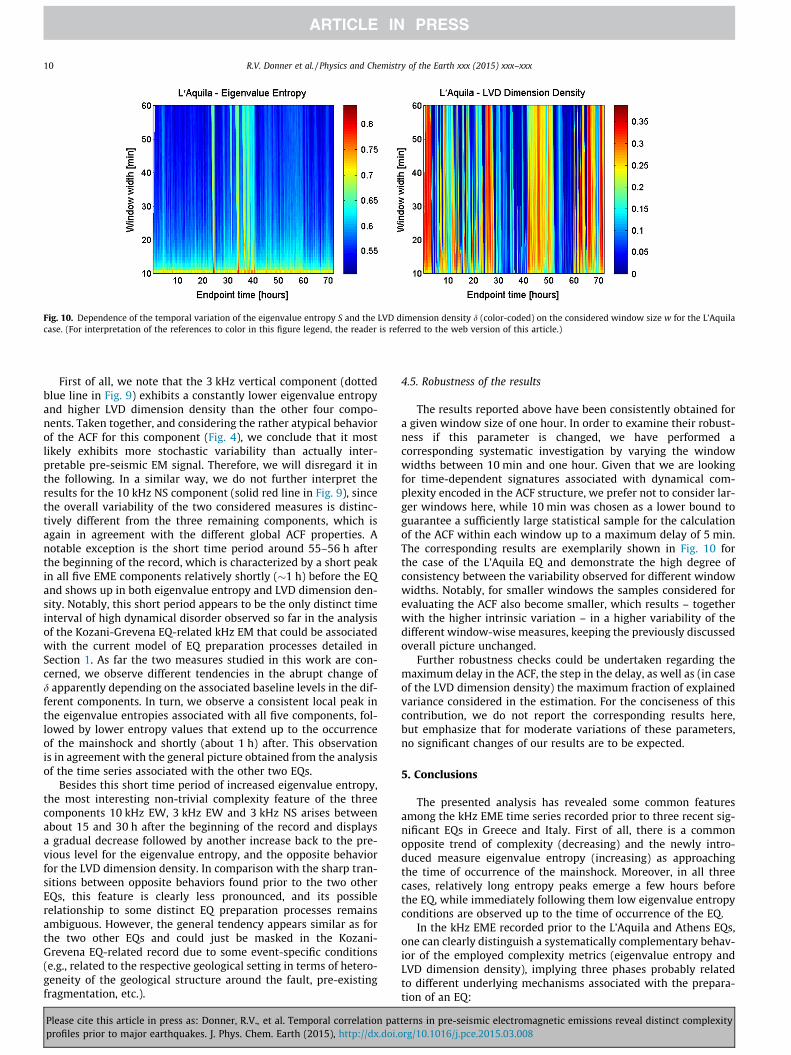
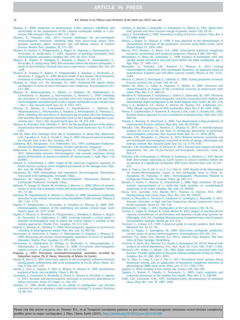
Fig. 10. Dependence of the temporal variation of the eigenvalue entropy S and the LVD dimension density d (color-coded) on the considered window size w for the L’Aquilacase. (For interpretation of the references to color in this figure legend, the reader is referred to the web version of this article.)


First of all, we note that the 3 kHz vertical component (dottedblue line in Fig. 9) exhibits a constantly lower eigenvalue entropyand higher LVD dimension density than the other four compo-nents. Taken together, and considering the rather atypical behaviorof the ACF for this component (Fig. 4), we conclude that it mostlikely exhibits more stochastic variability than actually inter-pretable pre-seismic EM signal. Therefore, we will disregard it inthe following. In a similar way, we do not further interpret theresults for the 10 kHz NS component (solid red line in Fig. 9), sincethe overall variability of the two considered measures is distinc-tively different from the three remaining components, which isagain in agreement with the different global ACF properties. Anotable exception is the short time period around 55–56 h afterthe beginning of the record, which is characterized by a short peakin all five EME components relatively shortly (�1 h) before the EQand shows up in both eigenvalue entropy and LVD dimension den-sity. Notably, this short period appears to be the only distinct timeinterval of high dynamical disorder observed so far in the analysisof the Kozani-Grevena EQ-related kHz EM that could be associatedwith the current model of EQ preparation processes detailed inSection 1. As far the two measures studied in this work are con-cerned, we observe different tendencies in the abrupt change ofd apparently depending on the associated baseline levels in the dif-ferent components. In turn, we observe a consistent local peak inthe eigenvalue entropies associated with all five components, fol-lowed by lower entropy values that extend up to the occurrenceof the mainshock and shortly (about 1 h) after. This observationis in agreement with the general picture obtained from the analysisof the time series associated with the other two EQs.

Besides this short time period of increased eigenvalue entropy,the most interesting non-trivial complexity feature of the threecomponents 10 kHz EW, 3 kHz EW and 3 kHz NS arises betweenabout 15 and 30 h after the beginning of the record and displaysa gradual decrease followed by another increase back to the pre-vious level for the eigenvalue entropy, and the opposite behaviorfor the LVD dimension density. In comparison with the sharp tran-sitions between opposite behaviors found prior to the two otherEQs, this feature is clearly less pronounced, and its possiblerelationship to some distinct EQ preparation processes remainsambiguous. However, the general tendency appears similar as forthe two other EQs and could just be masked in the Kozani-Grevena EQ-related record due to some event-specific conditions(e.g., related to the respective geological setting in terms of hetero-geneity of the geological structure around the fault, pre-existingfragmentation, etc.).


4.5. Robustness of the results

The results reported above have been consistently obtained fora given window size of one hour. In order to examine their robust-ness if this parameter is changed, we have performed acorresponding systematic investigation by varying the windowwidths between 10 min and one hour. Given that we are lookingfor time-dependent signatures associated with dynamical com-plexity encoded in the ACF structure, we prefer not to consider lar-ger windows here, while 10 min was chosen as a lower bound toguarantee a sufficiently large statistical sample for the calculationof the ACF within each window up to a maximum delay of 5 min.The corresponding results are exemplarily shown in Fig. 10 forthe case of the L’Aquila EQ and demonstrate the high degree ofconsistency between the variability observed for different windowwidths. Notably, for smaller windows the samples considered forevaluating the ACF also become smaller, which results – togetherwith the higher intrinsic variation – in a higher variability of thedifferent window-wise measures, keeping the previously discussedoverall picture unchanged.

Further robustness checks could be undertaken regarding themaximum delay in the ACF, the step in the delay, as well as (in caseof the LVD dimension density) the maximum fraction of explainedvariance considered in the estimation. For the conciseness of thiscontribution, we do not report the corresponding results here,but emphasize that for moderate variations of these parameters,no significant changes of our results are to be expected.

5. Conclusions

The presented analysis has revealed some common featuresamong the kHz EME time series recorded prior to three recent sig-nificant EQs in Greece and Italy. First of all, there is a commonopposite trend of complexity (decreasing) and the newly intro-duced measure eigenvalue entropy (increasing) as approachingthe time of occurrence of the mainshock. Moreover, in all threecases, relatively long entropy peaks emerge a few hours beforethe EQ, while immediately following them low eigenvalue entropyconditions are observed up to the time of occurrence of the EQ.

In the kHz EME recorded prior to the L’Aquila and Athens EQs,one can clearly distinguish a systematically complementary behav-ior of the employed complexity metrics (eigenvalue entropy andLVD dimension density), implying three phases probably relatedto different underlying mechanisms associated with the prepara-tion of an EQ:




(i) A first characteristic phase of intermittent fluctuations in theeigenvalue entropy dominates a time interval of a few tensof hours prior to the mainshock. This phase is characterizedby a relatively low initial baseline level of eigenvalueentropy and a high initial baseline level of dynamical com-plexity, which exhibit gradual trends towards higherentropy and lower complexity.

(ii) A second phase is characterized by extended periods of lowdynamical complexity and high eigenvalue entropy, whichcan be interrupted by time intervals of opposite characteris-tics. This second phase is terminated shortly (a few hours)prior to the EQ. As suggested by our findings for theL’Aquila EQ, the first two phases may at least partiallyoverlap.

(iii) The final phase is characterized by a state of low eigenvalueentropy and high complexity following right after the sec-ond phase, persisting up to the time of occurrence of theEQ and possibly beyond.

The first phase could be a manifestation of the fracture of pre-existing fragments filling the gap between the rough profiles ofthe fault, while the second appears consistent with the signaturesto be expected for a fracture of the strong entities (asperities) sus-taining the system. The last phase signalizes the preparation of thedynamical slip, which results in the fast, even super-shear, modethat surpasses the shear wave speed and is perceived as the mainEQ event. The first two phases fall into the third stage of thefour-stage model of the EQ preparation process by means of frac-ture-induced EME mentioned in Section 1, providing a finerpartitioning of this stage consistent with other already publishedresults (Minadakis et al., 2012). In turn, the third phase would beconsistent with the fourth stage of the aforementioned model.

In terms of the employed complexity metrics, the kHz EMErecorded prior to the Kozani-Grevena EQ behave differently fromthose prior to the L’Aquila and Athens EQs, not clearly presentingall the above features. This finding could be due to the differentshape of the corresponding spectra as a result of different dataquality, as suggested by the presented analysis, or to differentdynamics related to the different geological structure around thecorresponding focal volumes. It is noted that the power spectrumof the Kozani-Grevena kHz activity reveals two different power-laws, one for the low frequencies and another for the high frequen-cies [Fig. 4 in Kapiris et al. (2004)]. The high frequency power-lawmay reflect the dynamics within the bursts of the kHz emissionswhile the low frequency one may indicate the correlation betweenthe bursts. It should also be noted that the lead-time and the dura-tion of the detected kHz EM anomaly before the Kozani-GrevenaEQ were much shorter than in the other two cases, especially com-pared to the Athens kHz EME. These differences are probably aresult of the fact that the Kozani-Grevena focal area has a morehomogeneous geological structure, while it is less fragmented,since the Kozani-Grevena is a region of low historical seismic activ-ity (Contoyiannis et al., 2015).

We emphasize that the presented analysis provides first indica-tions for a refinement of the mechanistic model of EQ preparationprocesses through temporal correlation patterns in pre-seismicelectromagnetic emissions and the associated distinct complexityprofiles. Due to the limited amount of data considered here forthe pre-mainshock period, we cannot yet draw any final conclu-sions about whether or not the herein revealed complexity andeigenvalue entropy signatures are truly unique to the preparatorystages of major EQs. However, to this end we do not have anyresults supporting the occurrence of similar patterns outside theEQ preparation process. A corresponding analysis will be subjectof future work. In addition, we underline the necessity of a furtherin-depth characterization of the three identified phases by means


of complementary statistical as well as nonlinear dynamics tools,such as breakpoint regression for the observed trends in complex-ity and eigenvalue entropy or a deeper investigation of the scalingcharacteristics of the kHz EME during the different phases and therelevant time-scales involved in them by means of, e.g., waveletanalysis. We are confident that such future analyses can help fur-ther constraining the physical mechanisms underlying thereported temporal complexity profiles and may thus provideanother important step towards a better understanding of EQ pre-paration processes.

Conflict of interest

The authors declare no conflict of interest.

Acknowledgements

This work has been financially supported by the joint Greek-German project ‘‘Transdisciplinary assessment of dynamicalcomplexity in magnetosphere and climate: A unified descriptionof the nonlinear dynamics across extreme events’’ funded by IKYand DAAD. RVD acknowledges additional support by the GermanFederal Ministry for Education and Research via the BMBF YoungInvestigator’s Group CoSy-CC2 (Grant no. 01LN1306A). Technicalassistance by M. Wiedermann in performing the presentednumerical analyses was very much appreciated. GB acknowledgesadditional support from the European Union Seventh FrameworkProgramme (FP7-REGPOT-2012-2013-1) under grant agreementno. 316210 (BEYOND – Building Capacity for a Centre ofExcellence for EO-based monitoring of Natural Disasters).

References

Antonopoulos, G., 1996. Modeling the geoelectric structure of Zante Island from MTmeasurements. Ph. D. thesis, University of Athens (in Greek).

Baddari, K., Frolov, A., 2010. Regularities in discrete hierarchy seismo-acoustic modein a geophysical field. Ann. Geophys. 53, 31–42.

Baddari, K., Frolov, A., Tourtchine, V., Rahmoune, F., 2011. An integrated study of thedynamics of electromagnetic and acoustic regimes during failure of complexmacrosystems using rock blocks. Rock Mech. Rock Eng. 44, 269–280.

Ben-David, O., Cohen, G., Fineberg, J., 2010. The dynamic of the onset of frictionalslip. Science 330, 211–214.

Broomhead, D.S., King, G.P., 1986. Extracting qualitative dynamics fromexperimental data. Physica D 20, 217–236.

Carpinteri, A., Lacidogna, G., Manuello, A., Niccolini, G., Schiavi, A., Agosto, A., 2012.Mechanical and electromagnetic emissions related to stress-induced cracks.SEM Exp. Techniq. 36, 53–64.

Chang, J., Lockner, D., Reches, Z., 2012. Rapid acceleration leads to rapid weakeningin earthquake-like laboratory experiments. Science 338, 101–105.

Chauhan, V., Misra, A., 2008. Effects of strain rate and elevated temperature ofelectromagnetic radiation emission during plastic deformation and crackpropagation in ASTM B 265 grade 2 Titanium sheets. J. Math. Sci. 43, 5634–5643.

Cicerone, R.D., Ebel, J.E., Britton, J., 2009. A systematic compilation of earthquakeprecursors. Tectonophysics 476, 371–396.

Contoyiannis, Y., Eftaxias, K., 2008. Tsallis and Levy statistics in the preparation ofan earthquake. Nonlin. Proc. Geophys. 15, 379–388.

Contoyiannis, Y.F., Kapiris, P.G., Eftaxias, K.A., 2005. A Monitoring of a pre-seismicphase from its electromagnetic precursors. Phys. Rev. E 71, 066123.

Contoyiannis, Y., Potirakis, S.M., Eftaxias, K., Contoyianni, L., 2015. Tricriticalcrossover in earthquake preparation by analyzing preseismic electromagneticemissions. J. Geodyn. 84, 40–54.

Donner, R.V., Balasis, G., 2013. Correlation-based characterisation of time-varyingdynamical complexity in the Earth’s magnetosphere. Nonlin. Proc. Geophys. 20,965–975.

Donner, R., Witt, A., 2006. Characterisation of long-term climate change bydimension estimates of multivariate palaeoclimatic proxy data. Nonlin. Proc.Geophys. 13, 485–497.

Donner, R., Witt, A., 2007. Temporary dimensions of multivariate data frompaleoclimate records – a novel measure for dynamic characterization of long-term climate change. Int. J. Bifurcation Chaos 17, 3685–3689.

Donner, R., Sakamoto, T., Tanizuka, N., 2008. Complexity of spatio-temporalcorrelations in Japanese air temperature records. In: Donner, R.V., Barbosa,S.M. (Eds.), Nonlinear Time Series Analysis in the Geosciences – Applications inClimatology, Geodynamics, and Solar-Terrestrial Physics. Springer, Berlin, pp.125–154.


http://refhub.elsevier.com/S1474-7065(15)00032-7/h0005











































Eftaxias, K., 2009. Footprints of nonextensive Tsallis statistics, selfaffinity anduniversality in the preparation of the L’Aquila earthquake hidden in a pre-seismic EM emission. Physica A 389, 133–140.

Eftaxias, K., Potirakis, S.M., 2013. Current challenges for pre-earthquakeelectromagnetic emissions: shedding light from micro-scale plastic flow,granular packings, phase transitions and self-affinity notion of fractureprocess. Nonlin. Proc. Geophys. 20, 771–792.

Eftaxias, K., Kapiris, P., Polygiannakis, J., Bogris, N., Kopanas, J., Antonopoulos, G.,Peratzakis, A., Hadjicontis, V., 2001. Signature of pending earthquake fromelectromagnetic anomalies. Geophys. Res. Lett. 28, 3321–3324.

Eftaxias, K., Kapiris, P., Dologlou, E., Kopanas, J., Bogris, N., Antonopoulos, G.,Peratzakis, A., Hadjicontis, 2002. EM anomalies before the Kozani earthquake: astudy of their behavior through laboratory experiments. Geophys. Res. Lett. 29,1228.

Eftaxias, K., Frangos, P., Kapiris, P., Polygiannakis, J., Kopanas, J., Peratzakis, A.,Skountzos, P., Jaggard, D., 2004. Review-model of pre-seismic electromagneticemissions in terms of fractal-electrodynamics. Fractals 12, 243–273.

Eftaxias, K., Panin, V.E., Ye, Deryugin Ye., 2007. Evolution-EM signals beforeearthquakes in terms of meso-mechanics and complexity. Tectonophysics 431,273–300.

Eftaxias, K., Athanasopoulou, L., Balasis, G., Kalimeri, M., Nikolopoulos, S.,Contoyiannis, Y., Kopanas, J., Antonopoulos, G., Nomicos, C., 2009. Unfoldingthe procedure of characterizing recorded ultra low frequency, kHZ and MHzelectromagnetic anomalies prior to the L’Aquila earthquake as pre-seismic ones– Part 1. Nat. Hazards Earth Syst. Sci. 9, 1953–1971.

Eftaxias, K., Balasis, G., Contoyiannis, Y., Papadimitriou, C., Kalimeri, M.,Athanasopoulou, L., Nikolopoulos, S., Kopanas, J., Antonopoulos, G., Nomicos, C.,2010. Unfolding the procedure of characterizing recorded ultra low frequency,kHZ and MHz electromagnetic anomalies prior to the L’Aquila earthquake as pre-seismic ones – Part 2. Nat. Hazards Earth Syst. Sci. 10, 275–294.

Eftaxias, K., Potirakis, S.M., Chelidze, T., 2013. On the puzzling feature of the silenceof precursory electromagnetic emissions. Nat. Hazards Earth Syst. Sci. 13, 2381–2397.

Ghil, M., Allen, R.M., Dettinger, M.D., Ide, K., Kondrashov, D., Mann, M.E., Robertson,A.W., Saunders, A., Tian, Y., Varadi, F., Yiou, P., 2002. Advanced spectral methodsfor climatic time series. Rev. Geophys. 40, 3.

Gokhberg, M.K., Morgounov, V.A., Pokhotelov, O.A., 1995. Earthquake Prediction:Seismo-Electromagnetic Phenomena. Gordon and Breach, Singapore.

Hadjicontis, V., Mavromatou, C., Mastrogiannis, D., Antsygina, T.N., Chishko, K.A.,2011. Relationship between electromagnetic and acoustic emissions duringplastic deformation of gamma-irradiated LiF monocrystals. J. Appl. Phys. 110,024907.

Hansen, A., Schmittbuhl, J., 2003. Origin of the universal roughness exponent ofbrittle fracture surfaces:stress-weighted percolation in the damage zone. Phys.Rev. Lett. 90, 45504–45507.

Hayakawa, M., 1999. Atmospheric and Ionospheric Electromagnetic PhenomenaAssociated with Earthquakes. Terrapub, Tokyo.

Hayakawa, M., Fujinawa, Y., 1994. Electromagnetic Phenomena Related toEarthquake Prediction. Terrapub, Tokyo.

Johnson, P., Savage, H., Knuth, M., Gomberg, J., Marone, C., 2008. Effects of acousticwaves on stick-slip in granular media and implications for earthquakes. Nature451, 57–60.

Kalimeri, M., Papadimitriou, K., Balasis, G., Eftaxias, K., 2008. Dynamical complexitydetection in pre-seismic emissions using nonadditive Tsallis entropy. Physica A387, 1161–1172.

Kapiris, P., Polygiannakis, J., Peratzakis, A., Nomikos, K., Eftaxias, K., 2002. VHF-electromagnetic evidence of the underlying pre-seismic critical stage. EarthPlanets Space 54, 1237–1246.

Kapiris, P., Eftaxias, K., Nomikos, K., Polygiannakis, J., Dologlou, E., Balasis, G., Bogris,N., Peratzakis, A., Hadjicontis, V., 2003. Evolving towards a critical point: apossible electromagnetic way in which the critical regime is reached as therupture approaches. Nonlin. Proc. Geophys. 10, 511–524.

Kapiris, P., Eftaxias, K., Chelidze, T., 2004. Electromagnetic signature of prefracturecriticality in heterogeneous media. Phys. Rev. Lett. 92, 065702.

Karamanos, K., Peratzakis, A., Kapiris, P., Nikolopoulos, S., Kopanas, J., Eftaxias, K.,2005. Extracting pre-seismic electromagnetic signatures in terms of symbolicdynamics. Nonlin. Proc. Geophys. 12, 835–848.

Karamanos, K., Dakopoulos, D., Aloupis, K., Peratzakis, A., Athanasopoulou, L.,Nikolopoulos, S., Kapiris, P., Eftaxias, K., 2006. Pre-seismic electromagneticsignals in terms of complexity. Phys. Rev. E 74, 016104.

Kopanas, J., 1997. Precursory seismoelectromagnetic anomalies recorded byZakynthos station. Ph. D. thesis, University of Athens (in Greek).

Kumar, R., Misra, A., 2007. Some basic aspects of electromagnetic radiation emissionduring plastic deformation and crack propagation in Cu-Zn alloys. Mater. Sci.Eng. A 454, 203–210.

Kurths, J., Voss, A., Saparin, P., Witt, A., Kleiner, H., Wessel, N., 1995. Quantitativeanalysis of heart rate variability. Chaos 5, 88–94.

Lacidogna, G., Carpinteri, A., Manuello, A., Durin, G., Schiavi, A., Niccolini, G., Agosto,A., 2011. Acoustic and electromagnetic emissions as precursors phenomena infailure processes. Strain 47 (Suppl. 2), 144–152.

Lockner, D., 1996. Brittle fracture as an analog to earthquakes: can acousticemission be used to develop a viable prediction strategy? J. Acoustic Emission14, 88–101.


Lockner, D., Byerlee, J., Kuksenko, V., Ponomarev, A., Sidorin, A., 1991. Quasi-staticfault growth and shear fracture energy in granite. Nature 350, 39–42.

Lopez, J., Schmittbuhl, J., 1998. Anomalous scaling of fracture surfaces. Phys. Rev. E57, 6405–6408.

Makris, J., Bogris, N., Eftaxias, K., 1999. A new approach in the determination ofcharacteristic directions of the geoelectric structure using Mohr circles. EarthPlanets Space 51, 1059–1065.

Martin, M.T., Plastino, A., Rosso, O.A., 2006. Generalized statistical complexitymeasures: geometrical and analytical properties. Physica A 369, 439–462.

Matsumoto, H., Ikeya, M., Yamanaka, C., 1998. Analysis of barberpole color andspeckle noises recorded 6 and half hours before the Kobe earthquake. Jpn. J.App. Phys. 37, 1409–1411.

Minadakis, G., Potirakis, S.M., Nomicos, C., Eftaxias, K., 2012. Linkingelectromagnetic precursors with earthquake dynamics: an approach based onnonextensive fragment and self-affine asperity models. Physica A 391, 2232–2244.

Mourot, G., Morel, S., Bouchaud, E., Valentin, G., 2006. Scaling properties of mortarfracture surfaces. Int. J. Fract. 140, 39–54.

Müller, M., Baier, G., Galka, A., Stephani, U., Muhle, H., 2005. Detection andcharacterization of changes of the correlation structure in multivariate timeseries. Phys. Rev. E 71, 046116.

Nomikos, K., Vallianatos, F., Kaliakatsos, I., Sideris, E., Bakatsakis, M., 1997. The latestaspects of telluric and electromagnetic variations associated with shallow andintermediate depth earthquakes in the South Aegean. Ann. Geofis. 40, 361–374.

Peng, C.-K., Buldyrev, S.V., Havlin, S., Simons, M., Stanley, H.E., Goldberger, A.L.,1994. Mosaic organization of DNA nucleotides. Phys. Rev. E 49, 1685–1689.

Plerou, V., Gopikrishnan, P., Rosenow, B., Amaral, L.A.N., Guhr, T., Stanley, H.E., 2002.Random matrix approach to cross correlations in financial data. Phys. Rev. E 65,066126.

Ponson, L., Bonamy, D., Bouchaud, E., 2006. Two-dimensional scaling properties ofexperimental fracture surfaces. Phys. Rev. Lett. 96, 035506.

Potirakis, S.M., Minadakis, G., Nomicos, C., Eftaxias, K., 2011. A multidisciplinaryanalysis for traces of the last state of earthquake generation in preseismicelectromagnetic emissions. Nat. Hazards Earth Syst. Sci. 11, 2859–2879.

Potirakis, S.M., Minadakis, G., Eftaxias, K., 2012. Relation between seismicity andpre-earthquake electromagnetic emissions in terms of energy, information andentropy content. Nat. Hazards Earth Syst. Sci. 12, 1179–1183.

Potirakis, S.M., Karadimitrakis, A., Eftaxias, K., 2013. Natural time analysis of criticalphenomena: the case of pre-fracture electromagnetic emissions. Chaos 23,023117.

Potirakis, S.M., Contoyiannis, Y., Eftaxias, K., Koulouras, G., Nomicos, C., 2015. Recentfield observations indicating an Earth system in critical condition before theoccurrence of a significant earthquake. IEEE Geosc. Remote Sens. Lett. 12, 631–635.

Qian, S., Yian, J., Cao, H., Shi, S., Lu, Z., Li, J., Ren, K., 1994. Results of the observationson seismo-electromagnetic waves at two earthquake areas in China. In:Hayakawa, M., Fujinawa, Y. (Eds.), Electromagnetic Phenomena Related toEarthquake Prediction. Terrapub, Tokyo, pp. 205–211.

Renard, F., Voisin, C., Marsan, D., Schmittbuhl, J., 2006. High resolution 3D laserscanner measurements of a strike-slip fault quantity its morphologicalanisotropy at all scales. Geophys. Res. Lett. 33, L04305.

Rosso, O.A., Larrondo, H.A., Martin, M.T., Plastino, A., Fuentes, M.A., 2007.Distinguishing noise from chaos. Phys. Rev. Lett. 99, 154102.

Schiavi, A., Niccolini, G., Terrizzo, P., Carpinteri, A., Lacidogna, G., Manuello, A., 2011.Acoustic emissions at high and low frequencies during compression tests inbrittle materials. Strain 47, 105–110.

Shimamoto, T., Togo, T., 2012. Earthquakes in the Lab. Science 338, 54–55.Toonen, C., Lappe, D., Donner, R., Scholz-Reiter, B., 2012. Impact of machine-driven

capacity constellations on performance and dynamics of job-shop systems. In:ElMaraghy, H.A. (Ed.), Enabling Manufacturing Competetiveness and EconomicSustainability. Springer, Berlin, pp. 611–616.

Torrence, C., Compo, G.P., 1999. A practical guide to wavelet analysis. Bull. Amer.Meteorol. Soc. 79, 61–78.

Uyeda, S., Nagao, T., Kamogawa, M., 2009. Short-term earthquake prediction:current status of seismo-electromagnetics. Tectonophysics 470, 205–213.

Varotsos, P.A., Sarlis, N.V., Skordas, E.S., 2011a. Natural Time Analysis: The NewView of Time. Springer, Heidelberg.

Varotsos, P., Sarlis, N.V., Skordas, E.S., Uyeda, S., Kamogawa, M., 2011b. Natural timeanalysis of critical phenomena. Proc. Natl. Acad. Sci. U.S.A. 108, 11361–11364.

Warwick, J.W., Stoker, C., Meyer, T.R., 1982. Radio emission associated with rockfracture: Possible application to the great Chilean earthquake of May 22 1960. J.Geophys. Res. 87 (B4), 2851–2859.

Xie, X., Zhao, X., Fang, Y., Cao, Z., He, G., 2011. Normalized linear variance decaydimension density and its application of dynamical complexity detection inphysiological (fMRI) time series. Phys. Lett. A 375, 1789–1795.

Zapperi, S., 2010. Looking at how things slip. Science 330, 184–185.Zapperi, S., Kumar, P., Nukala, V., Simunovic, S., 2005. Crack roughness and

avalanche precursors in the random fuse model. Phys. Rev. E 71, 026106.Zoldi, S.M., Greenside, H.M., 1997. Karhunen-Loéve decomposition of extensive

chaos. Phys. Rev. Lett. 78, 1687–1690.




































































































































































temporal correlation patterns in pre-seismic...

Documents