temporal changes in the vagile epibenthic fauna of two

Vol. 5: 91-102, 1981 I MARINE ECOLOGY - PROGRESS SERIES Mar. Ecol. Prog. Ser. I Published April 30

Temporal Changes in the Vagile Epibenthic Fauna of Two Seagrass Meadows (Zostera capricorni and

Posidonia a ustralis)

P. C. Young

Division of Fisheries Research, CSIRO Marine Laboratories. P.O. Box 21, Cronulla, NSW 2230, Australia

ABSTRACT: The species richness, species conlposition, and abundance of species in samples of fish, crustaceans, and cephalopod molluscs were examined from samples collected from two monospecific seagrass meadows, Posidonia australis and Zostera capncorni. An analytical strategy is presented whereby the fauna were examined holistically by their full distribution of relative species occurrences and abundances. - Significant differences were demonstrated in both species composition and species abundance between the two seagrass meadows. Greatest differences in species composition occurred during times of low species richness, greatest differences in abundance during times of increased species richness. Within each year species were more often found, and in greater numbers, in summer than in winter, but annual variability was such that some species occurred so frequently and in a s great an abundance in summers of one year a s in winters of others. -The fauna of P. australis often contained the most species, and during a time of high salinity many species common to both meadows declined. However, a t that time a number of species characteristic of high salinity seagrass habitats showed increased frequencies in P. australis. - It was concluded that the differences in the fauna of the two seagrasses were controlled by external events leading to variable recruitment success. Only during favourable recruitment periods were the numbers of individuals different between the two meadows, whilst differences in species composition were heightened during periods of unfavourable recruitment for the dominant species.

INTRODUCTION

Stauffer (1937) found that, after mortality of the seagrass Zostera marina in a lagoon in Massachusetts USA, the only invertebrates remaining were those restricted to the surface of the mud and the infauna. All species previously found on or amongst the plants were absent, and the total number of species present had declined from 55 to 36. Since then the seagrass meadows have been widely recognized as a special- ised habitat, supporting a characteristic fauna. Hooks et al. (1976) described four distinct habitats for mac- roinvertebrates in the north eastern Gulf of Mexico, namely seagrass meadows, oyster beds, mud flats and benthic red algae, each of which was inhabited by a distinct group of species.

The animal communities of seagrass meadows were reviewed on a world wide basis by Kikuchi and Peres (1975), who indicated that a remarkable degree of parallelism occurred in these communities. They sug- gested, however, that local differences in species com-

O Inter-Research/Printed in F. R. Germany

position were related to the presence of different plant species, plant growth forms, physico-chemical environment, and climate and zoogeography. The first three of these factors are usually locally correlated with each other. This presents an often intractable difficulty in differentiating the relative importance of each factor to the distribution and abundance of the fauna associated with seagrass. Components of seagrass fauna have been described as (1) differentiating between geographical locations within one monospecific seagrass meadow (Heck, 1977; Brook, 1978); (2) characteristic of a particular species of seagrass (Kikuchi, 1961, 1974; Marsh, 1973; Weinstein and Heck, 1979); and (3) common to a number of seagrass species (Ledoyer, 1962).

In a previous study (Young and Wadley, 1979) shallow-water epibenthic macrofauna within an Australian subtropical estuarine system was examined. Differ- ences in the composition and abundance of epibenthic species in a range of seagrass species and bare substrates were related to the salinity/temperature

92 Mar Ecol. Prog. Ser. 5: 91-102, 1981

regime, water currents and often the depth of the substrate. The close relationship between the species composition of seagrass meadows and the depth of water in that area of study (Young and Kirkman, 1975) confused the precise role played by specific seagrass species in the determination of faunal change. In the present study the differences in juvenile and small epibenthic fish, vagile crustaceans and cephalopod molluscs were determined between two monospecific seagrass meadows [Zostera capricorni, Posidonia australis). By selecting two adjacent meadows with clearly recognizable substrate characteristics, but with similar depths and water properties, faunal variability associated with geographical changes was eliminated and the variability described here is attributable to the qualitative differences between the two seagrass species, and to time.

The two meadows were examined over a three year period between 1976 and 1979 in Port Hacking, N.S.W., Australia. By such a long study the temporal fluctuations in the epibenthic community could be examined, and compared to temporal changes in temperature, salinity and depth. Information was gathered on variability in species richness and occurrence and abundance of 51 epibenthic species from 216 samples. Examination of such a data set involves difficulties of sorting out information from random noise and a variety of methods have been used with mixed success In the past. Ever since Fisher et al. (1943) proposed the index a, most ecologists have attempted to summarise such data by a n lndex which attempts to describe a property of the community which condenses information on the number of species present, and the distribution of individuals amongst the species. The use of

such indices was critisized by Hurlbert (1971), however he then proceeded to formulate another two 'species composition parameters' Goodman (1975) pointed out the difficulties inherent in existing methods of data analysis, and May (1975) examined the concept of indices in this type of study. He concluded that communities should be described by their full distribution of relative specles abundances. The analysis of the present data set takes such a route and presents a n analytical method whereby such an examination is made.

METHODS

Sampling

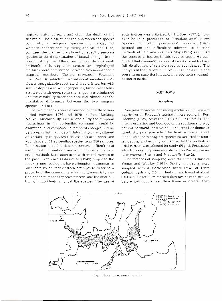
Seagrass meadows consisting exclusively of Zostera capricorni or Posidonia australis were found in Port Hacking (NSW, Australia, 34"04.6'S, 151°06.6'E). The area is estuarine and bounded on its southern shore by natural parkland, and without industrial or domestic input. An extensive intertidal bank where adjacent meadows of both seagrass species CO-occurred in similar depths, and equally influenced by the prevailing tidal current was selected for study (Fig. 1). Permanent sites for sampling were established on the seagrasses Z. capricorni (Site 1) and P. australis (Site 2).

The methods of sampling were the same as those of Young and Wadley (1979). Briefly, the fauna were sampled with a metre-wide beam trawl of l mm codend mesh and 2.5 mm body mesh, towed at about 0.04 m S-' over 50 m marked distance at each site. As before individuals less than 6 mm or greater than

Fig. 1 Location of sampling sites

Young: Temporal changes in the vagile epibenthic fauna 93

10 cm were discarded to eliminate net avoidance or escapement. The sampling of fauna was designed to eliminate as many variables as possible (except the differences in substrate) between sites. The sites were, therefore, sampled at monthly intervals, on the full moon, at night, within 0.5 h of full high tide, towing the net In the same direction relative to the current. Three consecutive trawls were taken from adjacent strips of substrate on each sampling occasion. The depth, temperature and salinity of the water at each site were measured before trawling.

Analysis

The samples were collected to use a three factor analysis of variance to detect significant variation between sites, months, and years. Variates examined were salinity, temperature, depth, species richness (number of species), species composition (actual species occurring), and species abundance (the distribution of the number of individuals of each species amongst the samples). Time serles analysis was not used because there was no a priori reason to assume that the biological data would follow any particular model, nor were there really sufficient number of data points.

U n i v a r i a t e d a t a . Of the variables examined, temperature, salinity, depth and species richness were univariate and presented no problems of analysis. The question of stabilizing the variance was addressed however.

Species richness data has usually been found to be Poisson distributed for which the appropriate transformation is the square root. This particular distribution was found in the present data when the variance and mean of a number of subsets were regressed against each other. The slope of the regression was close to 1 and the combined mean and variance values were almost equal. These data were therefore transformed to square roots prior to analysis.

The absence of replication in the environmental variables precluded any similar examination of mean and variance relationships for salinity, temperature, or depth. However, the relatively small range of each (27.8-35.7 %O S; 12.1-24.4 'C; 0.3-1.9 m) gave no evidence to suggest that the variance changed with the mean so here a transformation was not used.

M u l t i v a r i a t e d a t a . Each sample of the fauna may be envisaged as a vector of length S, the cells of which record the number of individuals collected in that sample of each of the s species present in the entire collection. All samples together form a matrix of s columns and n rows, where n equals the total number of samples in the collection. In the present study n

equals 3 (replicates) X 2 (sites) X 12 (months) X 3 (years) = 216; s equals the number of species occurring more than 5 times in the collection (51). The main interest was in the changes in frequency and abundance of species so those occurring less frequently than 5 times were deleted to reduce random variation, as it was felt that these rare species could contribute little to a n analysis of the three major factors (sites X years X

months). This matrix was then partitioned into two submat-

rices containing elther qualitative (presence/absence) or quantitative (numerical) data. The method whereby this partitioning was achieved is given later.

Each sample was thus described either qualitatively by all the presence/absences of s species; or quantita- tively by the abundances of the q species that it contained.

These descriptors were transformed by ordination prior to statistical analysis. By this technique each sample was considered to b e a point in space described uniquely by the combined values (binary or numerical) of the species. The points are then projected onto linear axes each of which describes a major linear combination of distributions possessed by groups of covarying species. Subsequent investigation of these projections by analysis of variance allows us to dis- criminate which distributions differentiate between the main factors under investigation (sites, months, years). The ordination technique used was that of Principal Coordinates Analysis, and the reasons for its use and its relationship to the more familiar Principal Components Analysis is detailed below.

I f , in an ecological study s species have been collected on n different sampling occasions the values may be entered as above into a n n X S matrix given by X. Each element X,, of this matrix is the observed value of the f h species on the ith sampling occasion. The point P, with rectangular cordinates (xi,, xiZ, .... X,,) can be considered as representing the ith sample in a space of s dimensions. By principal components analysis the line of best fit to the n points Pi (i = 1, 2 .... n) is obtained and the points Pi are all represented in one dimension by projecting them onto this line of best fit.

This line is calculated in such a way that the sum of squares of the perpendicular distances from each of the P, points onto the line is a t a minimum. Often with ecological data the species do not all distribute themselves through the samples in the same way and the Pi are not colinear. In this case successive lines of best fit may be calculated and the P, projected on them as well. Each line of best fit is calculated to pass through the centroid (origin) and the cosines which give it its direction are one of the latent roots of the sum of squares and products matrix (X'X). Of the s possible latent vectors we require for the first line that which

Mar. Ecol. Prog. Ser. 5: 91-102, 1981

extracts most of the variance. This is decided upon by The choice of measure is therefore implicit to the the size of the latent root corresponding to each latent information sought. vector. Because the sum of squares of the residuals is equal to the remaining latent roots, we extract that latent vector for which the corresponding latent root is Analysis of Species Composition greatest. The second, third, etc. lines of best fit are determined, if required, from the size of their respec- In the present case the initial data to be examined tive latent roots. consisted of a series of observations for each sample in

Principal components analysis is a widely used which the presence of a species was indicated by a 1

technique which has often been applied to ecological and its absence by a 0. The similarity measure most data. It possesses however, a number of features which appropriate for comparing frequency data is the infor- make it less attractive than otherwise might be the mation gain (Al ) on fusion of two samples (Williams, case; (1) unless all the variates (species) are measured 1976). This is a probabalistic measure (Lance and in the same scale, different results will be obtained for Williams, 1967) which measures the increase in a change of scale. This problem is usually avoided heterogeneity on fusion of two samples or groups of by prior data standardization. Williamson (1972) samples. If n samples are described by the presence or describes several such standardizations and discusses absence of s species and a, samples possess the jth their implications; (2) the procedure is inappropriate species and for binary (presence/absence) data. A variety of S

methods have been proposed to get round this problem I = sn In n - C [a , In aj + (n-a,) In (n-aj)] (Williamson, 1978) however, none can be considered ,= I completely satisfactory; (3) because of the usual use of then A I = I(p + g) - Ip - I q correlation coefficients in the calculation of latent roots where p and are the two samples to be and vectors, the absence of species from samples may This measure was calculated between all pairs of place samples close together whose only similarity is samples and used in the analysis of species composi- the joint absence of species. tion as the input matrix of similarity measures for

Gower (1967) described some of these weaknesses principal coordinates ~ ~ ~ l ~ ~ i ~ . and drew attention to a method (Principal Coordinates Analysis) whereby the projections of the Pi onto the lines of best fit could be calculated directly from an Analysis of Species Abundance analysis of a similarity matrix whose elements are d,, (Gower, 1966). These elements, d,, are a distance mea- Here the initial data on abundance were transformed sure between all pairs of samples, and the important to In (X + 1) prior to summation. This transformation new feature of the analysis is that any distance (or was used for two reasons: (1) The ordination extracts similarity) measure can be used for di, and the only linear trends in the data in a way analogous to regres- difficulty is to decide which is most appropriate. sion analysis. Many time varying aspects of abundance

Distance measures of this type have often been used are exponential in their effect (e.g. mortality rates), and to show similarities between all pairs of samples in a a logarithmic transformation will enable such trends to collection (e.g. Coleman et al., 1978). The major exhibit themselves in a linear manner. (2) The stan- advantage that Principal Coordinates analysis intro- dard deviation of animal populations is usually propor- duces is to refer the samples to principal axes (lines of tional to the mean and some form of transformation is best fit) and to thereby extract the major patterns of usually necessary prior to statistical analyses. In post- dissimilarity, due to covarying species, between the larval penaeid prawns, which are abundant in these samples. habitats the log transformation has been shown to be

All similarity measures indicate the extent to which appropriate (Young and Carpenter, 1977) for stabilis- samples share the same complement or abundances of ing the variance. Precise transformations for each species. The difference between any such index and species could have been calculated but this would community indices such as the Shannon-Weaver, is produce uninterpretable results and is inappropriate that the latter is compiled separately for each sample for present purposes. and does not differentiate between the sort of species Such a data matrix on the abundance of individuals present, nor which particular species the individuals of species with time, has usually been considered as belong to. Many similarity measures have been pro- containing quantitative data, and the calculation of posed and each, by its mathematical formulation, pos- similarity measures usually followed. Williams and sesses properties which may be more or less appropri- Dale (1962) showed, however, that this type of data ate as a measure of the feature of interest in the data. matrix contains not only numerical data, but also pre-


sence/absence data (which in this study is examined separately). They demonstrated that if in a set of values for some attribute (species), some of which are zero, be denoted by a vector [O,x] and m, is the mean of the non- zero values, then this vector can be partitioned into a qualitative vector [O,rn,], in which all non-zero values are replaced by m,, and a quantitative vector [O,x-m,] in which non-zero values are replaced by their difference from their mean. The division is a true partition between the qualitative and quantitative aspects of the information and their combined variances are equal to that of the original vector.

An all numeric data matrix was therefore con- structed by substituting the non-zero values for each species by their differences from their mean. By this substitution zero values are made equal to the mean of the non-zero values (0) and do not contribute to the similarity measure. Thus information about the abundance of a species is derived only from samples in which it occurs.

In this case a meristic measure of similarity is appropriate (Lance and Williams, 1967). The Gower metric was used and is given by:

where i , j = the samples under comparison; k = the species; W, = the range of the kth species in all the samples; s = the number of species; X = the abundance values. This measure can utilize the negative values which occur in the present data set, and this makes it more attractive than others in which negative values cannot be used. Other attractive properties of this measure are that, because each species is standar- dized by its range, it is a property of the entire population of each species under investigation, and its matrix has been shown to be ordinatable (Lance and Wil- liams, 1967).

In ordinations of both species composition and abundance the species most related to the patterns of dissimilarity revealed by the ordinations were extracted by correlating their input values with the scores on principal axes.

RESULTS

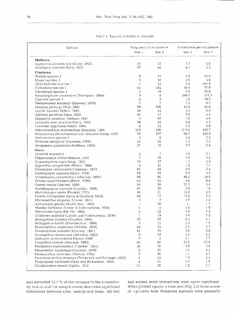
The species included in the analyses, together with their abundances and frequencies at each site, are given in Table 1. The results of the analysis of variance of major variables are presented in Table 2.

Environmental Conditions at the Sites

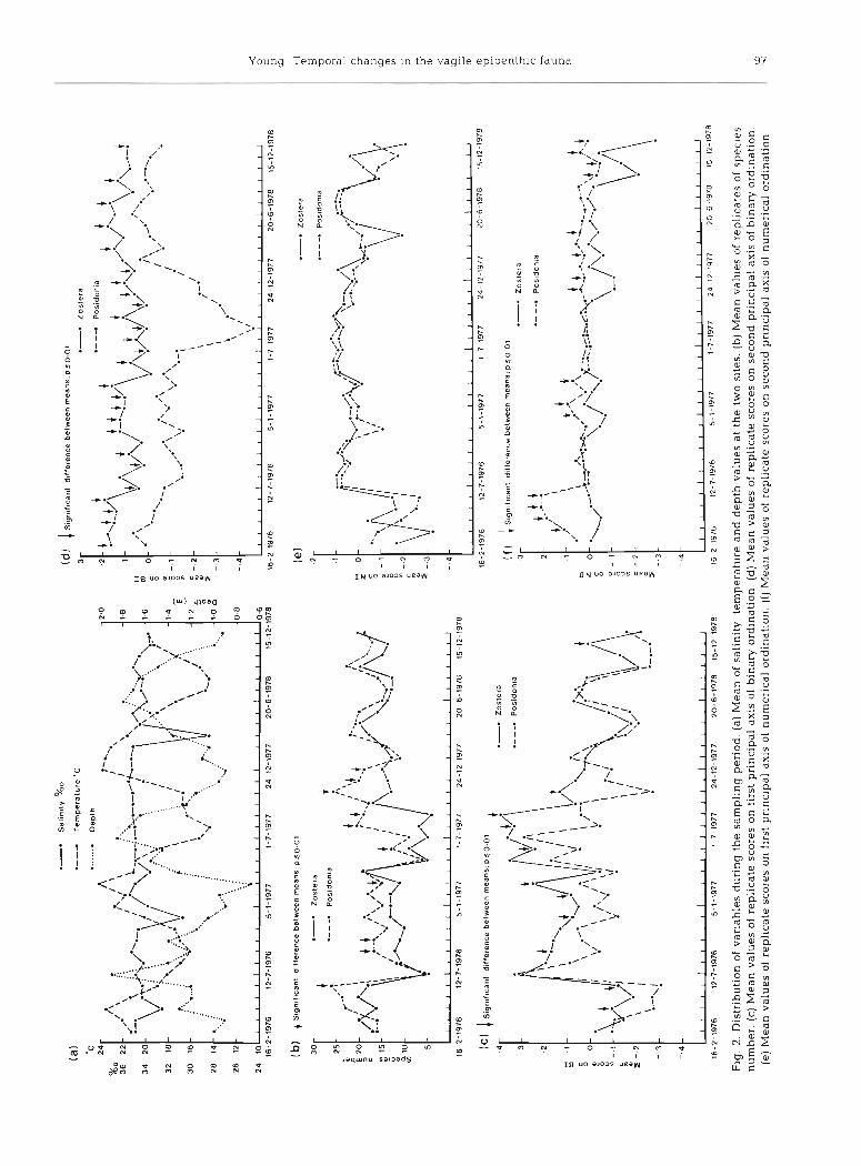
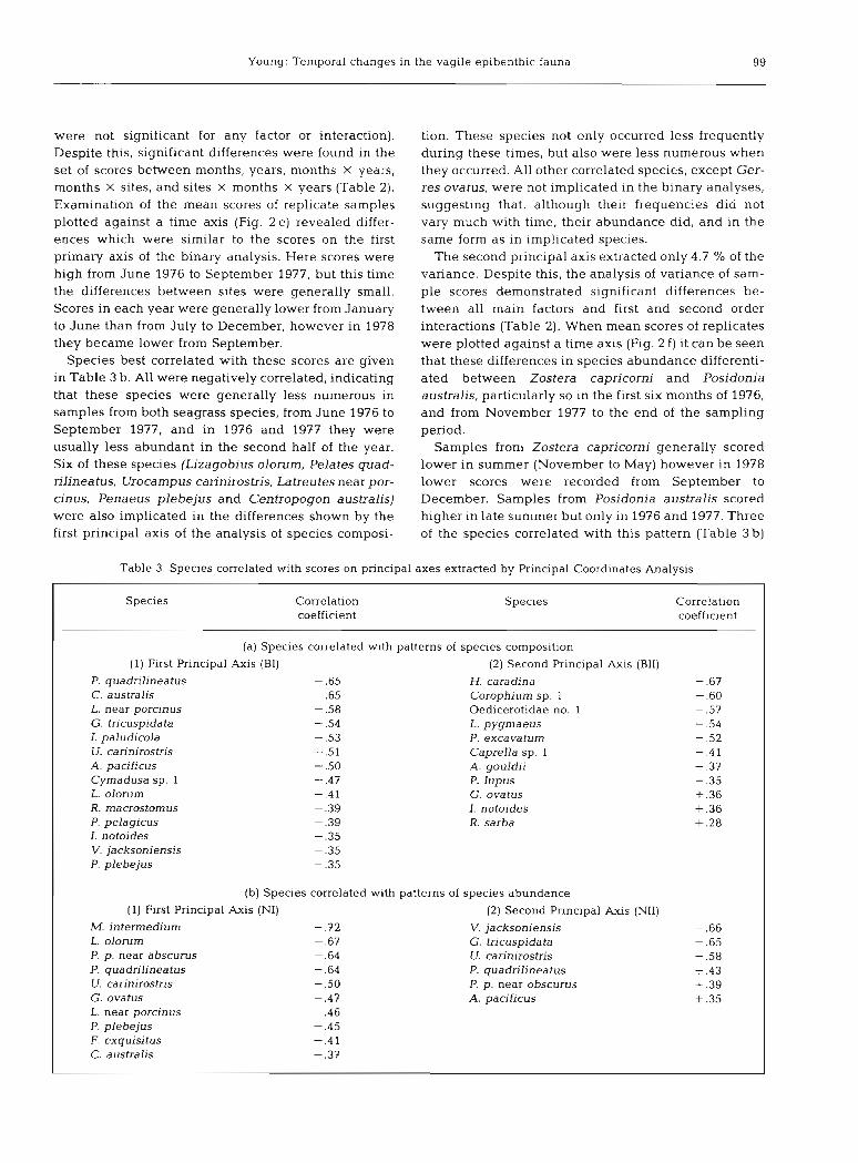
The analysis of variance of depth, salinity and temperature demonstrated that all three varied with months and years and that significant months X years interactions occurred (Table 2). Although the sites did not differ in water quality parameters (salinity, temperature) the Zostera capricorni site was significantly less deep than that of Posidonia australis. Although this depth difference was relatively consistent between months and years (about 10 cm) the differences in depths between the same month in each year, or different months in any one year was much greater than any difference between sites (Fig. 2a) . The same overall monthly changes occurred each year with minima in December to February, and maxima in June but con- siderable variation occurred from year to year.

The salinity at both sites showed the same monthly and yearly variability, but with no seasonal trends (Fig. 2a ) , and the changes were not consistent between years. Thus although a salinity drop occurred in March in all years, a second drop in November occurred only in 1976 and 1978.

The changes in temperature were common to both sites and in each year max.ima occurred from November to March, and minima in August (Fig. 2 a). The mean temperature in 1976 was higher than in the other two years and appeared to be due to warmer winter temperatures in that year.

Changes in the Fauna

The examination of species richness in the samples demonstrated (Table 2) that the number of species varied significantly with sites, months, and years, however both first and second order interaction terms were significant. Although more species were collected from Posidonia australis than Zostera capricorni during most months of each year (Fig. 2 b) significant differences between sites were not present in any month of 1978. At both sites the number of species declined in midwinter (June); however, the summer values for 1976-77 were similar to those of winter 1978. During such times the number of species collected from each seagrass meadow became more similar. From June 1976 there was an extended period of low species richness, especially in Z. capricorni, which lasted to September 1977. This extended decline was less apparent in P. australis.

The differences in species composition shown by sample scores on the first two principal axes of the ordination decribed two components of species composition which explained much of the difference described above in species richness. The first principal

96 Mar Ecol. Prog. Ser 5: 91-102, 1981

Table 1 Species included in analyses

Specles Frequency of occurrence Abundance per occurrence Site 1 Site 2 Site 1 Site 2

Mollusca : Euprymna stenodactyla (Grant, 1833) 43 31 l .7 1.6 Idlosepius notoides Berry, 1921 77 62 4.1 3.3

Crustacea: SirieIla species 1 8 11 4.9 11.9 Mysid number 1 2 10 2 5 4.8 Oedicerotidae number 1 4 12 2.5 107.9 Cymadusa species 1 83 102 14.0 77.8 Corophium species 1 3 19 3.0 19.8 Paracorophium excavatum (Thornpson, 1884) 3 8 106.7 171.3 Caprella species 1 2 5 1.0 18.2 Metapenaeus macleayi (Haswell, 1879) 5 7 1.2 6.7 Penaeus plebejus Hess, 1865 9 8 100 42.9 42.8 Lucifer hanseni Nobili, 1905 10 12 3.9 6.3 Alpheus pacificus Dana, 1852 4 3 51 2.0 4.4 Hippolyte caradina Holthuis, 1947 5 62 1.6 4.4 Latreutes near proclnus Kemp, 1916 3 8 64 3.4 4.3 Latreutes pygmaeus Nobili, 1904 8 51 2.0 4.8 Macrobrachiurn intermedium Stimpson, 1860 108 108 210.6 165.7 Periclimines (Per~climines] near obscurus Kemp, 1922 99 107 60.7 120.9 Halicarcinus species 1 3 6 1.0 2.2 Portunus pelagicus (Linnaeus, 1766) 14 24 1.2 1.5 Ilyograpsus paludicola (Rathbun, 1909) 3 7 50 2.7 6.4

Pisces Juvenile engraulid 2 7 1 .O 2.1 Hippocampus whitei Bleeker, 1855 7 28 1.0 1.2 Stigmatophora nigra Kaup, 1853 10 37 1.3 1.9 Sygnathus margaritifer (Peters, 1868) 4 10 1.0 1.1 Urocampus carinirostris Castelnau. 1872 62 48 3.8 2.4 Centropogon australis (Shaw, 1790) 68 93 2.9 3.2 Velambassis jacksoniensis (Macleay, 188 1) 98 86 56 2 14.0 Pelates quadrilineatus (Bloch, 1790) 63 9 1 5.6 8.6 Gerres ovatus Giinther, 1859 55 20 21.5 3.4 Acanthopagrus australis (Giinther, 1859) 4 1 30 1.8 1.9 Rhabdosargus sarba (Forskal, 1775) 49 3 1 12.0 5.0 Girella tricuspidata (Quoy & Gaimard, 1824) 68 72 12.0 7.3 Microcanthus strigatus (Cuvier, 1831) 3 7 1.7 1.3 Achoerodus gouldii (Richardson, 1843) - 26 1.7 Neodax balteatus (Cuvier & Valenciennes, 1839) 1 5 1.0 1 .O Petroscirtes lupus (De Vis . 1886) 3 33 1 .O 1.2 Cristiceps australis (Cuvier and Valenciennes, 1836) 1 19 1 0 1.2 Arenigobius frenatus (Giinther, 1861) 20 20 3.1 2.1 Bathygobius kreffti (Steindachner, 1866) 4 11 2.3 1.8 Favonogobius exquisitus (Whitley, 1950) 29 23 3.1 3.5 Favonogobius lateralis (Macleay, 1881) 4 1 20 5.0 2.8 Favongobius tamarensis (Johnston, 1882) 8 14 1.5 1.4 Gobiopterus sernivestita Munro, 1949 7 3 1.1 1.7 Llzagobius olorum (Sauvage, 1880) 80 80 21.6 12.9 Redlgoblus macrostomus (Giinther. 1861) 3 8 2 6 7.0 2.0 Meuschenia trachylepis (Giinther, 1870) 8 42 1.1 2.1 Monacanthus chinensis (Osbeck. 1765) 3 20 1.1 1.7 Paramonacanthus otisensis (Ternminck and Schlegel, 1850) 5 13 1 .O 1.5 Torquigener harniltoni (Gray and Richardson. 1843) 4 11 1.3 1.0 Dicotylicythys myersi Ogilby, 1910 14 18 1.2 1.1

axis extracted 12.7 % of the variance in the dissimilar- and second order interactions were again significant. ity matrix and the sample scores described significant When plotted against a time axis (Fig. 2 c) mean scores differences between sites, months and years. All first of replicates from Posidonia australis were generally

uo

~le

u~

p~

o

[estiamn

u jo srxe led!z~u!id p

uo

sas uo saioss a

le~

rlda

i JO san[eA

ue

aN

(l) ,uo

geu

!plo

les~

iau

rnu

10 s!xe [edrsu

rld ISI!J

uo

saloss a

les

~~

da

i jo san[eri u

ea

w (a)

,uo

~le

u~

p~

o

he

u~

q

jo srxe led

!su~

~d

p

uo

sas uo saloss a

leslld

a~

jo san[eA u

ea

w (p

) ,uo

rleutp

lo D

eu!q

jo slxe led!su!id ~

si!j uo saio3

s alestldal jo san[eA

ueapq (3

) .laqu

Inu

sa

pa

ds jo salesrld

ai 10 san[eA u

ea

w (q

) ,sal!s O

M~

aq

l le sanlen

qld

ap p

ue a

inle

~a

du

al 'A

l~u!les jo u

ea

w (e) .p

otlad

Butldures a

ql 6

u1

inp

salqe!IeA

jo uo

!lnq

~ils~

a

.Z .613

8L6L

-21-SL

9

L6

L-9

-02

L

L6I-Z

L-V

Z

LL

6I-L

-1

LL

SI-I-S

9

L6

L-L

-Zl

9L

6l-2

-91

I

Ji

11

11

~1

11

~l

~I

~I

~~

Ir

l~

ll

l~

lr

l,

1~

~~

I

;\

ela

iso

z .-.

T Joc

98 Mar Ecol. Prog. Ser. 5: 91-102. 1981

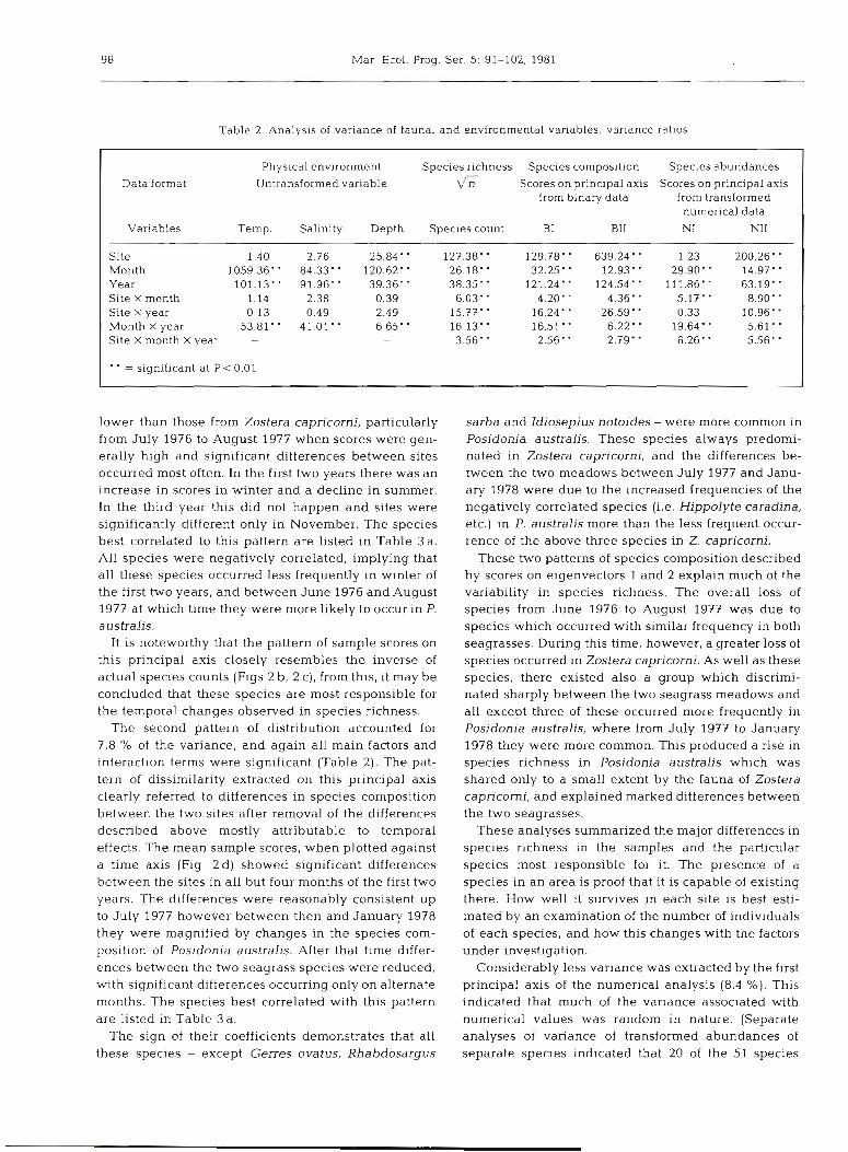
Table 2. Analysis of variance of fauna1 and environmental variables: variance ratios

Physical environment Species richness Species composition Spec~es abundances Data format Untransformed variable 6 Scores on principal axis Scores on principal axis

from binary data from transformed numerical data

Variables Temp. Salinity Depth Species count B I B11 NI NI1

Site 1.40 2.76 25.84 127.38. 129.78. 639.24 1.23 200.26- Month 1059.36' ' 84.33' ' 120.62' ' 26.18. 32.25 12.93' ' 29.90' 14.97. Year 101.13* 91.96" 39.36. - 38.35 121.24" 124.54 111.86" 63.19' ' Site X month 1.14 2.38 0.39 6.03. 4.20. 4.36. 5.17' 8.90 Site X year 0 13 0.49 2.49 15.77' ' 16.24' ' 26.59 0.33 10.96. Month X year 53.81 41.01 6.65- . 16.13. 16.51 6.22. 19.64- 5.61 ' ' Site X month X year - - - 3.56. 2.56 2.79- 6.26' 5.56'

.. _ significant at P < 0.01

lower than those from Zostera capricorni, particularly from July 1976 to August 1977 when scores were generally high and significant differences between sites occurred most often. In the first two years there was an increase in scores in winter and a decline in summer. In the third year this did not happen and sites were significantly different only in November. The species best correlated to this pattern are listed in Table 3 a . All species were negatively correlated, implying that all these species occurred less frequently in winter of the first two years, and between June 1976 and August 1977 at which time they were more likely to occur in P. a ustralis.

It is noteworthy that the pattern of sample scores on this principal axis closely resembles the inverse of actual species counts (Figs 2 b, 2 c), from this, it may be concluded that these species are most responsible for the temporal changes observed in species richness.

The second pattern of distribution accounted for 7.8 % of the variance, and again all main factors and interaction terms were significant (Table 2). The pattern of dissimilarity extracted on this principal axis clearly referred to differences in species composition between the two sites after removal of the differences described above mostly attributable to temporal effects. The mean sample scores, when plotted against a time axis (Fig. 2 d ) showed significant differences between the sites in all but four months of the first two years. The differences were reasonably consistent up to July 1977 however between then and January 1978 they were magnified by changes in the species composition of Posidonia australis. After that time differences between the two seagrass species were reduced, with significant differences occurring only on alternate months. The species best correlated with this pattern are listed in Table 3 a .

The sign of their coefficients demonstrates that all these species - except Gerres ovatus, Rhabdosargus

sarba and Idiosepius notoides -were more common in Posidonia australis. These species always predomi- nated in Zostera capricorni, and the differences between the two meadows between July 1977 and Janu- ary 1978 were due to the increased frequencies of the negatively correlated species (i.e. Hippolyte caradina, etc.) in P. australis more than the less frequent occurrence of the above three species in Z. capricorni.

These two patterns of species composition described by scores on eigenvectors 1 and 2 explain much of the variability in species richness. The overall loss of species from June 1976 to August 1977 was due to species which occurred with similar frequency in both seagrasses. During this time, however, a greater loss of species occurred in Zostera capricorni. As well as these species, there existed also a group which discrimi- nated sharply between the two seagrass meadows and all except three of these occurred more frequently in Posidonia australis, where from July 1977 to January 1978 they were more common. This produced a rise in species richness in Posidonia australis which was shared only to a small extent by the fauna of Zostera capricorni, and explained marked differences between the two seagrasses.

These analyses summarized the major differences in species richness in the samples and the particular species most responsible for it. The presence of a species in an area is proof that it is capable of existing there. How well it survives in each site is best esti- mated by an examination of the number of individuals of each species, and how this changes with the factors under investigation.

Considerably less variance was extracted by the first principal axis of the numerical analysis (8.4 %). This indicated that much of the variance associated with numerical values was random in nature. (Separate analyses of variance of transformed abundances of separate species indicated that 20 of the 51 species


were not significant for any factor or interaction). Despite this, significant differences were found in the set of scores between months, years, months X years, months X sites, and sites X months X years (Table 2) . Examination of the mean scores of replicate samples plotted against a time axis (Fig. 2 e ) revealed differences which were similar to the scores on the first primary axis of the binary analysis. Here scores were high from June 1976 to September 1977, but this time the differences between sites were generally small. Scores in each year were generally lower from January to June than from July to December, however in 1978 they became lower from September.

Species best correlated with these scores are given in Table 3 b. All were negatively correlated, indicating that these species were generally less numerous in samples from both seagrass species, from June 1976 to September 1977, and in 1976 and 1977 they were usually less abundant in the second half of the year. Six of these species (Lizagobius olorum, Pelates quadrilineatus, Urocarnpus carinirostris, Latreutes near porcinus, Penaeus plebejus and Centropogon australis) were also implicated in the differences shown by the first principal axis of the analysis of species composi-

tion. These species not only occurred less frequently during these times, but also were less numerous when they occurred. All other correlated species, except Ger- res ovatus, were not implicated in the binary analyses, suggesting that, although their frequencies did not vary much with time, their abundance did, and in the same form as in implicated species.

The second principal axis extracted only 4.7 % of the variance. Despite this, the analysis of variance of sample scores demonstrated significant differences between all main factors and first and second order interactions (Table 2). When mean scores of replicates were plotted against a time axis (Fig. 2 f ) it can be seen that these differences in species abundance differenti- ated between Zostera capricorni and Posidonia australis, particularly so in the first six months of 1976, and from November 1977 to the end of the sampling period.

Samples from Zostera capricorni generally scored lower in summer (November to May) however in 1978 lower scores were recorded from September to December. Samples from Posidonia australis scored higher in late summer but only in 1976 and 1977. Three of the species correlated with this pattern (Table 3 b)

Table 3. Species correlated with scores on principal axes extracted by Principal Coordinates Analysis

Species Correlation Species Correlation coefficient coefficient

(a) Species correlated with patterns of species composition

(1) First Principal Axis (BI) (2) Second Principal Axis (BII) P. quadrilineatus - .65 H. caradina - .67 C, australis - .65 Corophiurn sp. 1 - .60 L. near porcinus - .58 Oedicerotidae no. 1 - .57 G. tricuspida ta - .54 L. pygrnaeus - .54 I. paludicola - .53 P, excavatum - .52 U. carinirostris - .51 Caprella sp. 1 -.41 A. pacificus - .50 A. gouldii - .37 Cyrnadusa sp. 1 - .47 P. lupus - .35 L. olorurn -.41 G. ovatus + .36 R. rnacrostornus - .39 I. notoides + .36 P. pelagicus -.39 R. sarba + .28 I. notoides - .35 V. jacksoniensis - .35 P. plebejus - .35

(b) Species correlated with patterns of species abundance

(1) First Principal Axis (NI) (2) Second Principal Axis (NII) M. in termedium - .72 V. jacksoniensis - .66 L. olorum - .67 G. tricuspida ta - .65 P. p. near abscurus - .64 U. carinirostris - .58 P. quadnlineatus - .64 P. quadrilinea tus + .43 U. carinirostris - .50 P. p. near obscurus + .39 G. ovatus - .47 A. pacificus + .35 L. near porcinus - .46 P. plebejus - .45 F. exquisitus -.41 C. australis - .37

Mar. Ecol. Prog. Ser. 5: 91-102, 1981

were also implicated in the temporal changes in abundance demonstrated by scores of the first principal axis. The species, although sharing similar monthly and yearly differences in abundance, were more common in one or other of the two seagrass meadows. Velambassis jacksoniensis, Girella tricuspidata and Urocampus carinirostris were more abundant in Z. capricorni whereas Pelates quadrilineatus, Periclirnines p. near obscurus and Alphaeus pacificus were more abundant in Posidonia australis.

The species more abundant in Posidonia australis were more numerous in 1976, whereas those in Zostera capricorni were more numerous in 1978. From June 1976 to October 1977 all species were less numerous in both seagrass meadows and none showed the frequency differences between sites described by the second principal axis of the binary ordination.

DISCUSSION

The total variability accounted for in the analysis of species composition was 20.5 % and in the analysis of species abundance 13.1 %. These are both very low figures. Additional principal axes could have been extracted and samples projected onto them, however the purposes of the present study were to examine only the major trends of distribution and abundance in the collection. The fact that much of the variance remained unexplained serves to highlight the complexity of biological systems, and the magnitude of the inherent sampling error in any such field study. To adequately sample each species would require a sampling strategy specifically designed for each, and this would make interpretation and analysis of the data extremely difficult.

Despite the limitations imposed by the study, the major trends were extracted from the data by the present analytical methods. These trends referred to a reasonably large proportion of the species present, and described adequately the relationship of species composition and abundance to sites, months, and years.

The species examined in this study were mostly resident species (e.g. Macrobrachium intermedium, Centropogon australis) in which postlarval, juvenile, and adult forms CO-existed, or migratory species (e.g. Penaeus plebejus, Girella tricuspidata) in which only postlarval and juvenile forms occurred. Most species had pelagic larval stages, however a few (e.g. Urocam- pus carinirostris, Hippocampus whitei) incubated their eggs and did not have a pelagic stage to their life history.

The two seagrass meadows did not differ significantly with salinity or temperature, and the depth differences were small, and low compared with annual

variability. Despite this, Posidonia australis often had more species at any time during 1976 and 1977 than did Zostera capricorni. A large component of the fauna of both seagrass species showed similar temporal trends, marked by a decrease in both occurrence and abundance between June 1976 and August 1977. Some species did not show this trend, occurring predomin- antly in Posidonia australis especially so from July 1977 to January 1978.

Although many species were not more abundant in one or other of the two seagrass meadows, one component of the fauna did show a difference. This discrimi- nation occurred only at times of increased abundance (January to June 1976, and November 1977 to December 1978). The decline in abundance during the intervening period must have been due to effects which swamped favourable aspects of one seagrass meadow over the other. During times of low species richness (June 1976 to August 1977) no 'buffering' effect was detected on the decline in abundance by the presence of more species in Posidonia australis. What was apparent however, was that in P. australis other species occurred during that time, which were rare both in Zostera capricorni, and in P. australis during other times.

The general consistency of temporal change between both species of seagrass suggests that the species exhibiting such changes were responding to external stimuli common to both sites. The major temporal difference in both species composition and abundance referred to 1977 when the summer increase in both frequency of occurrence and abundance were lower than in other years. As mentioned previously, almost all recruitment of species to these seagrass beds originates from planktonic larvae which settle on the seagrasses for their demersal stages. In penaeid prawns the stimulus for settling has been shown to be the salinity change at the mouth of the estuary (Hughes, 1969). The winter/summer differences in abundance shown here were usually associated with a decrease in the size of individuals with increased abundance, and are most likely due to the settling of juveniles of the next generation from the plankton. From the present study it appears that a failure in recruitment was responsible for the trends observed. The consistently high salinity from March 1977 to February 1978 may well have contributed to lack of recruitment success. In Posidonia australis a number of species occurred during this time which were rare at other times. Amongst these species, Hippolyte caradina, Latreutes pygmaeus and Petroscirtes lupus have previously been shown to be characteristic of seagrass meadows located in areas of higher salinity (Young and Wadley, 1979).

Each species of seagrass meadow presents a habitat

Young: Temporal changes in the \.agile epibenthic fauna 101

which is qualitatively different, although both do have many features in common. As well as adding structural complexity to the environment both influence the phy- s ~ c a l and chemical constitutents of the substrate water. Both, by excretion and decay contribute materials to the milieu, their presence is associated with great bacterial activity (Baas Becking and Wood, 1955), and both contain reducing substances which may bring about reducing conditions in the substrate (Wood, 1953). In both species biomass increases, although not significantly, in summer and decreases in winter (Kirk- man and Reid, 1979), and their growth rates are strongly correlated with water temperature, and at a maximum in summer (Kirkman and Reid, unpubl.). Their epiphytic flora shows similar seasonal cycles with a change in species composition between winter and summer (May et al., 1979). However, differences also occur between the two seagrass species. Zostera capricorni is a much smaller plant and its rhizomes are much smaller. While the leaves of both species are heavily epiphytized - up to 71 % by dry weight of leaves of Posidonia australis may consist of epibiota (Kirkman and Reid, 1979) - algal epiphytes are more abundant on P. australis than on Z. capricorni (May et al . , 1979). In Zostera capricorni most leaves are shed in autumn; they float, and are displaced away from the bed in shore bands or in deeper water (Wood, 1959). In Posidonia australis, most leaves are shed in summer; they sink and are added to the organic detritus of the sediments. This leaf fall represents a potential resource which occurs in Posidonia australis but not Zostera capricorni.

Clearly, the resources offered by seagrasses present a habitat which many species recognize and utilize. Despite differences in fauna between Zostera capricorni and Posidonia australis, most temporal changes in abundance of species followed similar patterns in both meadows. Examination of both occurrence and abundances of species common to both seagrass meadows give no evidence of higher stability in the more diverse community (Posidonia australis). Rather do the fluctuations in species composition and abundance appear to be controlled by external stimuli common to both meadows.

Acknowledgements. I wish to thank Mr. D. D. Reid and Mr. R. L. Sandland for freely given statistical advice, and Ms. V. A. Wadley who supervised the field sampling and identification of the fauna.

LITERATURE CITED

Baas Becking, L. G. M., Wood, E. J. F. (1955). Biological processes in the estuarine environment. I. Ecology of the sulphur cycle. Proc. K. ned. Akad. Wet. 58: 160-181

Brook, I. V. (1978). Comparative macrofaunal abundance in turtle grass (Thalassja testudinum) communities in South Florida characterised by high blade density. Bull. mar Sci. Gulf Caribb. 28: 212-217

Coleman, N., Cuff, W., Drummond, M., Kudenov, J. D (1978). A quantitative survey of the rnacrobenthos of Western Port, Victoria. Aust. J. mar. Freshwat. Res. 29: 445-466

Fisher, R. A.. Corbet, A. S.. Williams, C . B. (1943). The relation between the number of individuals and the number of species In a random sample of an anlmal population. J . Anim. Ecol 12: 42-58

Goodman, D. (1975). The theory of diversity-stability relationship in ecology. Q. Rev. Biol. 50: 237-266

Gower, J. C. (1966). Some distance properties of latent root and vector methods used in multivariate analysis. Biornetrika 53: 325-328

Gower, J. C. (1967). Multivariate analysis and multidimen- sional geometry. Statistician 17: 13-28

Heck, K. L. (1977). Comparative species richness, composition, and abundance of invertebrates in Caribbean seagrass (Thalassia testud~num) meadows (Panama). Mar Biol. 41: 335-348

Hooks, T A., Heck, J r K. L., Livingston, R. J . (1976). An inshore marine invertebrate community: structure and habitat associations In the northeastern Gulf of Mexico. Bull. mar Sci. Gulf Caribb. 26: 99-109

Hughes, D. A. (1969). Responses of salinity change a s a tidal transport mechanism of pink shrimp Penaeus duorarum. Biol. Bull. mar biol. Lab.. Woods Hole 136: 43-53

Hurlbert, S H (1971). The nonconcept of species diversity: a critique and a l ternat~ve parameters Ecology 52: 577-586

Kikuchi, T (1961). An ecological study on animal community of Zostera belt, in Tomioka Bay, Amakusa, Kyushu. Com- munity composition (1) Fish fauna. Rec. oceanogr. Wks Japan, Spec. No. 5 : 21 1-219

Kikuchi, T. (1974). Japanese contributions on consumer ecology in eelgrass (Zostera marina L.) beds, with special reference to trophic relationships and resources in inshore fisheries. Aquaculture 4: 145-160

Kikuchi, T., Peres, J. M. (1975). A n ~ m a l com~nunities in the seagrass beds: a revlew. Review paper for the Consumer Ecology Working Group, International Seagrass Work- shop, Leiden, Netherlands, 1973. Contributions from the Amakusa Marine Biological Laboratory, Kyushi Uni- versity No. 227: 1-32

Kirkrnan, H , Reid, D D (1979). A study of the role of a seagrass Posidonia australis in the carbon budget of an estuary. Aquat. Bot. 7 - 173-183 .

Lance, G. N., Williams, W. T. (1967). Mixed-data classificat- ory programs. I. Agglomerative systems. Aust. Comp. J . 1: 15-20

Ledoyer, M. (1962). Etude de la faune vagile des herbiers superficiels des Zosteracees e t d e quelques biotopes d'al- gues littorales. Recl Trav. Stn mar. Endoume 25: 117-236

Marsh, G. A. (1973). The Zostera epifaunal community in the York River, Virginia. Chesapeake Sci. 14: 87-97

May, R. M. (1975). Successional patterns and indices of diversity. Nature, Lond. 258: 285-286

May, V., Collins, A. J., Collett, L. C. (1979). A comparative study of epiphytic algal communities on two common genera of sea-grasses in eastern Australia. Aust. J. Ecol. 3: 91-104

Stauffer, R. C. (1937). Changes in the invertebrate community of a lagoon after disappearance of the eelgrass. Ecology 18: 4 2 7 4 3 1

Weinstein, M. P,, Heck, K. L. (1979) Ichthyofauna of seagrass meadows along the Caribbean coast of Panama and in the

102 Mar. Ecol, h o g . Ser 5: 91-102. 1981

Gulf of Mexico: composition, structure and community ecology. Mar. Biol. 50: 97-107

Williams. W T (1976). Pattern analys~s in agricultural sci- ence, CSIRO/Elsevier, Melbourne

Williams, W. T., Dale, M. B. (1962). Partition correlation matrices for heterogeneous quantitative data. Nature, Lond. 196: 602

Williamson, M. (1972). The relation of principal Component Analysis to the Analysis of Variance. Int. J. Mat. Educ. Scl. Technol. 3: 35-42

Williamson, M. (1978). The ordination of incidence data. J. Eco~. 66: 911-920

Wood. E. J. (1953). Reducing substances in Zostera. Nature, Lond. 172: 916

Wood. E. J. (1959). Some East Australian sea-grass corn- munities. Froc. Linn. Soc. N.S.W. 84: 218-226

Young, P. C., Carpenter, S. M. (1977). Recruitment of postlarval penaeid prawns to nursery areas in Moreton Bay, Queensland. Aust. J. mar. Freshwat. Res. 28: 745-773

Young, P. C.. Kirkman, H. (1975). The seagrass communities of Moreton Bay, Queensland. Aquat. Bot. 1 - 191-202

Young, P. C., Wadley, V A. (1979). Distribution of shallow water epibenthic macrofauna in Moreton Bay, Queens- land, Australia. Mar. Biol. 53: 83-97

This paper was presented by Dr. G . F. Humphrey; it was accepted for printing on February 1. 1981

temporal changes in the vagile epibenthic fauna of two

Documents