energies

Article

Temperature Distribution in InsulatedTemperature-Controlled Container byNumerical Simulation

Bin Li 1, Jiaming Guo 1, Jingjing Xia 1,2, Xinyu Wei 1, Hao Shen 1, Yongfeng Cao 1, Huazhong Lu 3

and Enli Lü 1,*1 College of Engineering, South China Agricultural University, Guangzhou 510642, China;

ganli180@sina.com (B.L.); jmguo@scau.edu.cn (J.G.); ligan11221@163.com (J.X.); wxyscau@163.com (X.W.);sh1024384685@163.com (H.S.); 17864386076@163.com (Y.C.)

2 Schools of Automobile, Guangdong Mechanical and Electronical College of Technology,Guangzhou 510515, China

3 Guangdong Academy of Agricultural Sciences, Guangzhou 510640, China; huazlu@scau.edu.cn* Correspondence: enlilv@scau.edu.cn; Tel.: +86-020-8528-2860

Received: 7 August 2020; Accepted: 11 September 2020; Published: 12 September 2020�����������������

Abstract: Cold-storage containers are widely used in cold-chain logistics transportation due to theirenergy saving, environmental protection, and low operating cost. The uniformity of temperaturedistribution is significant in agricultural-product storage and transportation. This paper exploredtemperature distribution in the container by numerical simulation, which included ventilationvelocity and the fan location. Numerical model/numerical simulation showed good agreement withexperimental data in terms of temporal and spatial air temperature distribution. Results showedthat the cooling rate improved as velocity increased, and temperature at 45 min was the lowest,when velocity was 16 m/s. Temperature-distribution uniformity in the compartment became worsewith the increase in ventilation velocity, but its lowest temperature decreased with a velocity increase.With regard to fan energy consumption, the cooling rate of the cooling module, and temperature-fielddistribution in the product area, velocity of 12 m/s was best. Temperature standard deviation andnonuniformity coefficient in the container were 0.87 and 2.1, respectively, when fans were located inthe top four corners of the container. Compared with before, the average temperature in the box wasdecreased by 0.12 ◦C, and the inhomogeneity coefficient decreased by more than twofold. The resultsof this paper provide a better understanding of temperature distribution in cold-storage containers,which helps to optimize their structure and parameters.

Keywords: computational fluid dynamics; numerical analysis; cold-storage container; temperaturedistribution; optimization; cold chain

1. Introduction

The development of cold-chain transportation was facilitated by population growth and theincreasing demand of consumers for fresh food [1]. Refrigerated trucks are an important link of foodtransportation, and the most common mode of transportation in a cold chain [2,3].

At present, diesel-engine-driven mechanical steam-compression refrigeration is still the maintechnology of cold-chain land transportation [4]. This kind of refrigeration has high noise, maintenancecosts, and CO2 emissions, and its efficiency is only 35–40% [5], causing such refrigerated vehiclesconfronted with restrictions when they deliver in large cities [1]. Phase-change materials (PCMs) canchange their physical state over a range of temperatures, releasing and storing large amounts of energyduring melting or solidification, thus changing the temperature of the surrounding environment [6–9].

Energies 2020, 13, 4765; doi:10.3390/en13184765 www.mdpi.com/journal/energies

Energies 2020, 13, 4765 2 of 16

They are widely used in various cold-storage and cold-transportation systems [10–15]. Due to theirenergy-saving, environmental protection, and low operating cost advantages, refrigerated storagevehicles are increasingly favored by transport operators [4,16]. Cold-storage vehicles mainly releasetheir cold quantity through natural and forced convection [4,16–18]. Both cooling methods are subjectto local supercooling and poor temperature uniformity in the container.

A number of studies showed that the uneven distribution of refrigerating capacity in refrigeratedcontainers still poses significant challenges to product freshness and quality in long-distancetransportation and harsh environments [19–22]. Reasonable temperature distribution can ensure theeven distribution of the cooling capacity, save energy consumption, reduce dry consumption andfreeze-damage loss, and improve the quality of fresh fruit [23]. Therefore, it is necessary to improve thedistribution of the cooling capacity of fruit transport equipment. In general, temperature uniformitymainly depends on the external environment and internal air circulation [24]. The most direct way toreduce the influence of external ambient temperature fluctuations on internal temperature is to improvecontainer insulation performance. Many scholars proposed to replace part of the polyurethane foamwith a vacuum heat shield with a lower heat-transfer coefficient [25–27] to improve the insulation of thevessel and the utilization rate of the internal space. The main factors affecting internal air circulationare the design of refrigerated containers, the perforation rate of cargo packaging, the way in whichpackages are stacked, and pallet configuration [20]. However, it is very time-consuming and laboriousto obtain an optimal parametric solution of internal air-flow optimization by experiment.

Computational fluid dynamics (CFD) modeling is an alternative to expensive and cumbersomeexperiments, and the primary method for analyzing flow and temperature fields in fruit storageand transportation [28,29]. Many studies modeling air-flow patterns and temperature distributionin refrigeration rooms demonstrated the appropriateness of this approach. The authors in [30] usednumerical simulation and experiment methods to study the influence of the presence or absence ofa supply air-duct system for ventilation performance and temperature uniformity in the container.Results showed that the air-duct system could improve overall ventilation uniformity in the containerand reduce cargo temperature difference. In order to reduce the loss of cold air flow, the authors in [20]added three diversion plates to the refrigerated container to prevent air flow from passing throughthe air gap. Compared with before the improvement, temperature distribution was within ±1 ◦C,and cooling time was also reduced by at least 22.9%. Kayansayan et al. [31] numerically analyzed theconjugate heat transfer in the refrigerated container, and the effects of the container shape, inlet channelwidth, and Reynolds number of cold air on temperature distribution. Jara et al. [32] used a CFDshear–stress transfer calculation model to simulate temperature distribution in a specific refrigeratorvehicle, and studied the refrigeration cycle in the cold space of the vehicle at a lower cost. Han et al. [33]used 3D CFD models to simulate air flow and heat transfer under different unsteady-turbulence models,and predicted temporal and spatial temperature and velocity changes during cooling. In terms of theapplication of cold storage, Yang et al. [34] verified the feasibility of combining cold storage with latentheat storage by using a CFD model, and carried out a simulation analysis on the temperature-distributionand heat-transfer characteristics of cold storage. In addition, Xie et al. [35] analyzed the influence ofdifferent cold-plate layouts on the temperature-field distribution in no-load refrigerated vehicles byusing computational fluid dynamics combined with experiment verification.

Previous studies on CFD modeling and simulations of refrigeration space lack research onthe location of fans and air velocity inside the container, especially for storage refrigerators withlimited cold-source cooling capacity. Air-flow velocity and distribution have great influence on theheat-exchange rate of the storage module and the cargo area, so it is necessary to study the location ofthe fan and air velocity inside the storage refrigerator.

This study revealed the temperature distribution in a container by a validated CFD model. Besides,the performance of four velocities and four locations of the fan were compared to explore the influenceof operating parameters on temperature distribution. The results of this research provided reliablereferences of container optimization in the cold chain.

Energies 2020, 13, 4765 3 of 16

2. Materials and Methods

2.1. Materials

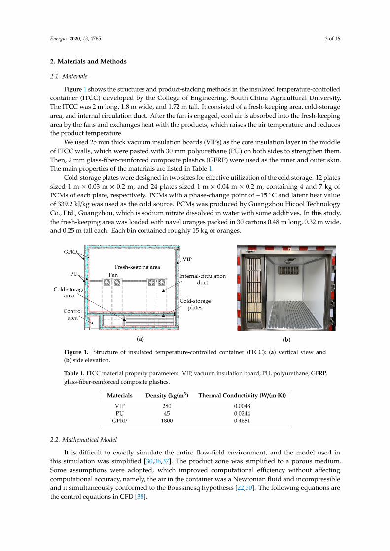
Figure 1 shows the structures and product-stacking methods in the insulated temperature-controlledcontainer (ITCC) developed by the College of Engineering, South China Agricultural University.The ITCC was 2 m long, 1.8 m wide, and 1.72 m tall. It consisted of a fresh-keeping area, cold-storagearea, and internal circulation duct. After the fan is engaged, cool air is absorbed into the fresh-keepingarea by the fans and exchanges heat with the products, which raises the air temperature and reducesthe product temperature.

We used 25 mm thick vacuum insulation boards (VIPs) as the core insulation layer in the middleof ITCC walls, which were pasted with 30 mm polyurethane (PU) on both sides to strengthen them.Then, 2 mm glass-fiber-reinforced composite plastics (GFRP) were used as the inner and outer skin.The main properties of the materials are listed in Table 1.

Cold-storage plates were designed in two sizes for effective utilization of the cold storage: 12 platessized 1 m × 0.03 m × 0.2 m, and 24 plates sized 1 m × 0.04 m × 0.2 m, containing 4 and 7 kg ofPCMs of each plate, respectively. PCMs with a phase-change point of −15 ◦C and latent heat valueof 339.2 kJ/kg was used as the cold source. PCMs was produced by Guangzhou Hicool TechnologyCo., Ltd., Guangzhou, which is sodium nitrate dissolved in water with some additives. In this study,the fresh-keeping area was loaded with navel oranges packed in 30 cartons 0.48 m long, 0.32 m wide,and 0.25 m tall each. Each bin contained roughly 15 kg of oranges.

Energies 2020, 13, x FOR PEER REVIEW 3 of 16

2. Materials and Methods

2.1. Materials

Figure 1 shows the structures and product-stacking methods in the insulated temperature-controlled container (ITCC) developed by the College of Engineering, South China Agricultural University. The ITCC was 2 m long, 1.8 m wide, and 1.72 m tall. It consisted of a fresh-keeping area, cold-storage area, and internal circulation duct. After the fan is engaged, cool air is absorbed into the fresh-keeping area by the fans and exchanges heat with the products, which raises the air temperature and reduces the product temperature.

We used 25 mm thick vacuum insulation boards (VIPs) as the core insulation layer in the middle of ITCC walls, which were pasted with 30 mm polyurethane (PU) on both sides to strengthen them. Then, 2 mm glass-fiber-reinforced composite plastics (GFRP) were used as the inner and outer skin. The main properties of the materials are listed in Table 1.

Cold-storage plates were designed in two sizes for effective utilization of the cold storage: 12 plates sized 1 m × 0.03 m × 0.2 m, and 24 plates sized 1 m × 0.04 m × 0.2 m, containing 4 and 7 kg of PCMs of each plate, respectively. PCMs with a phase-change point of −15 °C and latent heat value of 339.2 kJ/kg was used as the cold source. PCMs was produced by Guangzhou Hicool Technology Co., Ltd., Guangzhou, which is sodium nitrate dissolved in water with some additives. In this study, the fresh-keeping area was loaded with navel oranges packed in 30 cartons 0.48 m long, 0.32 m wide, and 0.25 m tall each. Each bin contained roughly 15 kg of oranges.

(a)

(b)

Figure 1. Structure of insulated temperature-controlled container (ITCC): (a) vertical view and (b) side elevation.

Table 1. ITCC material property parameters. VIP, vacuum insulation board; PU, polyurethane; GFRP, glass-fiber-reinforced composite plastics.

Materials Density (kg/m3) Thermal Conductivity (W/(m·K)) VIP 280 0.0048 PU 45 0.0244

GFRP 1800 0.4651

2.2. Mathematical Model

It is difficult to exactly simulate the entire flow-field environment, and the model used in this simulation was simplified [30,36,37]. The product zone was simplified to a porous medium. Some assumptions were adopted, which improved computational efficiency without affecting computational accuracy, namely, the air in the container was a Newtonian fluid and incompressible

Figure 1. Structure of insulated temperature-controlled container (ITCC): (a) vertical view and(b) side elevation.

Table 1. ITCC material property parameters. VIP, vacuum insulation board; PU, polyurethane; GFRP,glass-fiber-reinforced composite plastics.

Materials Density (kg/m3) Thermal Conductivity (W/(m·K))

VIP 280 0.0048PU 45 0.0244

GFRP 1800 0.4651

2.2. Mathematical Model

It is difficult to exactly simulate the entire flow-field environment, and the model used inthis simulation was simplified [30,36,37]. The product zone was simplified to a porous medium.Some assumptions were adopted, which improved computational efficiency without affectingcomputational accuracy, namely, the air in the container was a Newtonian fluid and incompressibleand it simultaneously conformed to the Boussinesq hypothesis [22,30]. The following equations arethe control equations in CFD [38].

Energies 2020, 13, 4765 4 of 16

(1) Continuity equation:∂ρ f

∂t+∇ · (ρ f

→υ ) = Sm, (1)

where ρf is the fluid density in kg/m,→υ is the velocity vector in m/s, and Sm is the source term for mass

generation in kg/(m3·s), Sm is zero. The increase in mass should be equal to the mass flux. Buoyancy

force [39] increases as a result of density variation per the assumption that only the effects of thebuoyancy term and temperature on fluid density were considered; other effects were ignored [40].

(2) Momentum equation:

∂(ρ f→υ )

∂t+∇ · (ρ f

→υ→υ ) = −∇p + ρ f

→g + S j, (2)

where p is the static pressure in Pa and→g is the gravitational force in N/m3. Sj is the source term for the

j-th (x, y, or z) momentum equation, which is given by

S j =µ

αυ j + C2(

12ρυ

∣∣∣υ j∣∣∣), (3)

where 1/α is the viscous drag coefficient and C2 is the inertial resistance coefficient.The wall treatment in this paper was enhanced to consider the effect of wall roughness on air flow.

The wall-enhancement function can be incorporated into the models by establishing a viscous model.(3) Energy equation:

∂∂t(φρ f E f + (1−φ)ρpEp) + ∇ · (

→υ (ρ f E f + p)) = ∇ · ke f f · ∇T −

∑i

hi→

Ji + Shf , (4)

where φ is the porosity of the medium, Ef is the fluid energy in J/kg, Ep is the product energy in J/kg,

hi is the enthalpy of species i in J/kg,→

J i is the diffusion flux in kg/(m2·s), Sh

f is the enthalpy source term

in W/m3, and keff is the effective thermal conductivity of the porous medium in W/(m·K) that can bedefined as

ke f f = φk f + (1−φks), (5)

where kf is the fluid-phase thermal conductivity (including turbulence) in W/(m·K), and ks is thesolid-medium thermal conductivity in W/(m·K).

Temperature distribution in cold-storage containers is related to the heat-insulation performance ofinsulation materials, which includes vacuum insulation boards and polyurethanes. Thermal-insulationperformance of storage and temperature-controlled containers can be defined as Equations (6)–(8) [41]:

Rw =1α1

+∑ x j

λ j+

1α2

, (6)

where Rw is the heat resistance of the storage and temperature-controlled container in m2·◦C/W, λj is

the thermal conductivity of heat-transfer materials in each layer in W/(m·K), xj is the thickness of eachmaterial layer in m, α1 is the heat-transfer coefficient of the inner surface of the container in W/(m2

·K),and α2 is the heat-transfer coefficient of the outer surface of the container in W/(m2

·K). The containerheat transfer coefficients of the inner and outer surfaces are generally calculated by Equations (7) [42]:

αi = 1.163× (4 + 12√

vi) (7)

Ki =1

Rw, (8)

Energies 2020, 13, 4765 5 of 16

where αi is the convection heat-transfer coefficient between the wall surface of the container and theair in W/(m2

·K), vi is air-flow velocity inside or outside the container in m/s, and Ki is the heat-transfercoefficient of each surface of the container in W/(m2

·K). The total heat transfer coefficient K of thecontainer is calculated by Formula (9) [42]:

K =

S∑i=1

KiAi

S∑i=1

Ai

, (9)

Ai =√

Ai1Ai2. (10)

where Ai is the total heat transfer area of container, Ai1 and Ai2 are the geometric heat transfer areainside and outside the container respectively. Considering the influence of the thermal bridge andsealing on the total heat transfer coefficient, it is necessary to modify the total heat transfer coefficient ofthe container [43]. The correction factor for this article is 1.15, provided by the container manufacturer.The applicable thermal properties of air were obtained from FLUENT (2003).

Appropriate boundary conditions must be exactly established in this model. The fan outlet wasassumed to be the velocity inlet, and the outlet was assumed to be the pressure outlet. Velocity wasconstant in both inlets as per the boundary conditions for Equations (1) and (2). Velocity in the fan outletcould be stated as υx = 0, υy = υ, υz = 0. In this model, υ was calculated on the basis of Equation (1).The UDF was used to represent the change of inlet temperature with time under different velocitylevels, and data were experimentally obtained (Figure 2). For the produce space, υ was affected bythe resistance of the produce and its package; this resistance was calculated by using Equation (3).Boundary condition details are shown in Table 2. Viscous resistance and inertial resistance wereobtained by measuring the products’ ventilation resistance, which was represented by the pressuredifference in different velocity, and then it was synthesized to a one variable quadratic equation withno intercept. The hole rate is 0.3, viscous resistance is 19,441, and inertial resistance is 0.05891 bymeasuring and calculating. Due to the impact of forced convection intensity, the inlet temperature ofthe fan varied with time, the entry boundary cannot be set to the same parameter. Thus, relationshipbetween the air velocity and inlet air temperature, and a user-defined function (UDF) between the twowas added into the model. The heat load outside the container was also considered, and its heat transfercoefficient was calculated to 0.13734 W/m2K by Equation (6) to Equation (10). Average temperature ofoutside the container within 45 min was tested to represent the wall temperature in the CFD model.

Table 2. Details of boundary conditions.

Name Inlet Outlet Products Wall

Boundary condition Velocity inlet Pressure outlet Porous zone ConvectionVelocity (m/s) 16 - - -

Temperature (K) UDF 281.15 - 308.15Pressure (Pa) - 0 - -

Viscous resistance (1/m2) - - 19,441 -Inertial resistance (1/m) - - 0.06 -

Heat transfer coefficient (W/m2K) - - - 0.13734

Energies 2020, 13, 4765 6 of 16Energies 2020, 13, x FOR PEER REVIEW 6 of 16

Figure 2. User-defined function (UDF) equation of the inlet temperature over time.

2.3. Numerical Method

The length, width, and height of the computational domain, which was developed with CATIA software, were 1.78, 1.17, and 1.49 m, respectively. A hexahedral mesh was used to discretize the model in ICEM-CFD (integrated computer engineering and manufacturing code for computational fluid dynamics) software due to its higher computational accuracy. All of the physical parameters of each element were calculated by the finite-volume method, including velocity, pressure, and temperature. The mesh density of the inlet, outlet, and product surface was improved for greater computational accuracy.

The independence of the generated mesh by ICEM-CFD is very important when simulated in FLUENT. Mesh size is the main reason for direct error accumulation [44,45]. Additionally, large mesh size also significantly slows down calculation efficiency. Therefore, it is necessary to determine proper mesh size, which helps to enhance computation efficiency and calculation accuracy. This part mainly aims to ensure mesh accuracy by monitoring the average velocity of different computational domains and the velocity of the location of the monitor sensor. The number of cells generated by ICEM-CFD ranges from initially 100,000 to approximately 1,000,000 by changing max and min cell size, including local refinement.

Figure 3 shows the schematic of measuring points. Figure 4a shows the average temperature of 15 measuring points and space average temperature in ITCC. Average temperature fluctuated slightly as the number of cells changed from 100,000 to 500,000. It was also obvious that there was a gentle velocity incline of the monitor sensor in the area from 670,000 to 950,000, which testified that the number of cells in this area was suitable for simulation in FLUENT. Considering the computational power requirement, a smaller number of cells was selected in this task. A 3D mesh file with 670,000 cells was constructed for this research. The mesh model is shown in Figure 4b.

y = 25.89e-0.026x

y = -6.6787Ln(x) + 30.798

y = -6.585ln(x) + 28.917

y = -5.602ln(x) + 22.539

-5

0

5

10

15

20

25

30

35

0 300 600 900 1200 1500 1800 2100 2400 2700

Tem

pera

ture

/℃

Time /s

4 m/s8 m/s12 m/s16 m/sFitted equation(4 m/s)Fitted equation(8 m/s)Fitted equation(12 m/s)Fitted equation(16 m/s)

Figure 2. User-defined function (UDF) equation of the inlet temperature over time.

2.3. Numerical Method

The length, width, and height of the computational domain, which was developed withCATIA software, were 1.78, 1.17, and 1.49 m, respectively. A hexahedral mesh was used todiscretize the model in ICEM-CFD (integrated computer engineering and manufacturing code forcomputational fluid dynamics) software due to its higher computational accuracy. All of the physicalparameters of each element were calculated by the finite-volume method, including velocity, pressure,and temperature. The mesh density of the inlet, outlet, and product surface was improved for greatercomputational accuracy.

The independence of the generated mesh by ICEM-CFD is very important when simulated inFLUENT. Mesh size is the main reason for direct error accumulation [44,45]. Additionally, large meshsize also significantly slows down calculation efficiency. Therefore, it is necessary to determineproper mesh size, which helps to enhance computation efficiency and calculation accuracy. This partmainly aims to ensure mesh accuracy by monitoring the average velocity of different computationaldomains and the velocity of the location of the monitor sensor. The number of cells generated byICEM-CFD ranges from initially 100,000 to approximately 1,000,000 by changing max and min cell size,including local refinement.

Figure 3 shows the schematic of measuring points. Figure 4a shows the average temperature of15 measuring points and space average temperature in ITCC. Average temperature fluctuated slightlyas the number of cells changed from 100,000 to 500,000. It was also obvious that there was a gentlevelocity incline of the monitor sensor in the area from 670,000 to 950,000, which testified that thenumber of cells in this area was suitable for simulation in FLUENT. Considering the computationalpower requirement, a smaller number of cells was selected in this task. A 3D mesh file with 670,000 cellswas constructed for this research. The mesh model is shown in Figure 4b.

Energies 2020, 13, 4765 7 of 16

Energies 2020, 13, x FOR PEER REVIEW 7 of 16

Figure 3. Schematic of measuring points.

(a)

(b)

Figure 4. Results of the mesh-independence study: mesh (a) independence and (b) model.

4

6

8

10

101.206 181.006 310.592 414.828 467.422 670.79 931.592

Tem

pera

ture

/℃

Mesh size/ (10^3)

Mean temperature at 15 points

Space average temperature

Figure 3. Schematic of measuring points.

Energies 2020, 13, x FOR PEER REVIEW 7 of 16

Figure 3. Schematic of measuring points.

(a)

(b)

Figure 4. Results of the mesh-independence study: mesh (a) independence and (b) model.

4

6

8

10

101.206 181.006 310.592 414.828 467.422 670.79 931.592

Tem

pera

ture

/℃

Mesh size/ (10^3)

Mean temperature at 15 points

Space average temperature

Figure 4. Results of the mesh-independence study: mesh (a) independence and (b) model.

The Reynolds number (Re) depends on the form of the fluid, and it is a significant variable forsimulation, related to selecting a turbulence model. In this study, this variable was calculated usingEquation (11) [46]:

Energies 2020, 13, 4765 8 of 16

Re = UL/ν, (11)

where U is the characteristic scale of velocity, m/s, L is the characteristic scale of length, m, and v is thekinematic viscosity, m2/s.

Large eddy simulation (LES) is an important means for studying turbulent motion. It has beenused in many studies to analyze turbulence under simple geometries and boundary conditions [47–49].Due to the large computational cost, LES has not been widely applied in engineering. In previous CFDmodels [43,49], the k–ε turbulent model was widely used to solve high Re value cases, which wereexperimentally verified with high accuracy. Therefore, this study used the standard k–ε model for itslower computational consumption. Turbulence intensity (I) was needed for CFD simulation, which wascalculated by Equation (12) [50]:

I = 0.16(Re)−1/8. (12)

Computations were performed with an AMD Ryzen 7 PRO 1700 eight-core processor with a 16 GBRAM. The CFD code of this work was Fluent 18.2 with a finite volume approach. A pressure-base modelwas used for calculation because fluid density had little change. A steady solver was used to initializethe fluid field before using a transient solver, and initialization was done when its convergence ofcontinuity, momentum, and energy reached 10−3, 10−3, and 10−6, respectively. Gravitational accelerationwas also considered and it was set to be −9.81 m/s2. The time step of this case was set as 1 × 10−4 s,with 20 iterations in each time step.

The coefficient of inhomogeneity (COI) was used to evaluate the distribution uniformity oftemperature in the container, which could be defined [35] as

S =n∑i

∣∣∣(ti − tn)/tn∣∣∣, (13)

where S is the coefficient of inhomogeneity; ti is the temperature of ith sensor, ◦C; and tn is the averagetemperature of n sensors, ◦C.

2.4. Physical Model

Four groups of air velocity and four groups of fan locations were selected for numerical analysisto optimize temperature distribution in the container. Air velocity was 4, 8, 12, and 16 m/s, respectively.The specific locations of the fan are shown in Figure 5. In all cases, the same parameters, solutionmethod, initial conditions, and boundary conditions were used.

Energies 2020, 13, x FOR PEER REVIEW 8 of 16

The Reynolds number (Re) depends on the form of the fluid, and it is a significant variable for simulation, related to selecting a turbulence model. In this study, this variable was calculated using Equation (11) [46]:

Re /UL ν= , (11)

where U is the characteristic scale of velocity, m/s, L is the characteristic scale of length, m, and v is the kinematic viscosity, m2/s.

Large eddy simulation (LES) is an important means for studying turbulent motion. It has been used in many studies to analyze turbulence under simple geometries and boundary conditions [47–49]. Due to the large computational cost, LES has not been widely applied in engineering. In previous CFD models [43,49], the k–ε turbulent model was widely used to solve high Re value cases, which were experimentally verified with high accuracy. Therefore, this study used the standard k–ε model for its lower computational consumption. Turbulence intensity (I) was needed for CFD simulation, which was calculated by Equation (12) [50]:

1/80.16(Re)I −= . (12)

Computations were performed with an AMD Ryzen 7 PRO 1700 eight-core processor with a 16 GB RAM. The CFD code of this work was Fluent 18.2 with a finite volume approach. A pressure-base model was used for calculation because fluid density had little change. A steady solver was used to initialize the fluid field before using a transient solver, and initialization was done when its convergence of continuity, momentum, and energy reached 10–3, 10–3, and 10–6, respectively. Gravitational acceleration was also considered and it was set to be −9.81 m/s2. The time step of this case was set as 1 × 10–4 s, with 20 iterations in each time step.

The coefficient of inhomogeneity (COI) was used to evaluate the distribution uniformity of temperature in the container, which could be defined [35] as

( ) /n

i n ni

S t t t= − , (13)

where S is the coefficient of inhomogeneity; ti is the temperature of ith sensor, °C; and tn is the average temperature of n sensors, °C.

2.4. Physical Model

Four groups of air velocity and four groups of fan locations were selected for numerical analysis to optimize temperature distribution in the container. Air velocity was 4, 8, 12, and 16 m/s, respectively. The specific locations of the fan are shown in Figure 5. In all cases, the same parameters, solution method, initial conditions, and boundary conditions were used.

(a)

(b)

Figure 5. Cont.

Energies 2020, 13, 4765 9 of 16

Energies 2020, 13, x FOR PEER REVIEW 9 of 16

(c)

(d)

Figure 5. Specification of different fan locations: (a) L0; (b) L1; (c) L2; and (d) L3.

2.5. Experimental Research

Experiments were carried out in the ITCC (1:1 scale as the container) with cold-storage and temperature-control transportation. These experiments served to verify the accuracy of the simulation models. Temperature and air velocity were recorded by fifteen thermocouples and fifteen hot wire anemometers respectively. On the basis of the results of a previous analysis, the locations of these sensors were determined and are shown in Figure 3. Thermocouples (CHT-D version) with a measuring range of −20–80 °C and accuracy of ±0.3 °C were used. Hot wire anemometers (CHWVN WD4150) with a measuring velocity range of 0–30 m/s and accuracy 0.02% of the read value and resolution of 0.01 m/s were used.

The navel oranges used in the experiment were purchased from a Jiangnan fruit wholesale market in Guangzhou and transported to the College of Engineering of South China Agricultural University by refrigerated transportation. In order to ensure the quality of the navel oranges, they were carefully graded, and damaged and inferior-quality samples were eliminated. Before the experiments, the cold-storage plate was fully frozen in −20 °C cold storage, and the oranges were precooled to 8 °C; then, the oranges and cold-storage plate were quickly moved to the cold-storage area to start the temperature-control experiment. The temperature-control interval was set to 2–8 °C. The sensors were connected to a data-recording instrument with a data-recording interval of 10 s.

3. Results

3.1. Model Verification

Figure 6a shows the difference of experimental air velocity and simulation air velocity, where the maximal and minimal air velocity difference between the experiment and simulated air velocity was 0.59 and 0.02 m/s, respectively, and the average air velocity difference was 0.11 m/s. The experimental air velocity ranged from 0.28 to 6.86 m/s while simulation air velocity ranged from 0.18 to 7.0 m/s. Temperature data of 15 sensors were obtained when the monitor sensor had reached 2 °C after 45 min. Figure 6b shows the difference of the experimental temperature and simulation temperature. Figure 6b shows that the maximal and minimal temperature difference between the experiment and simulated temperatures was 2.1 and 0.12 °C, respectively, and the average temperature difference was 0.9 °C. The experimental temperature ranged from 0.3 to 5.2 °C while the simulation temperature ranged from 0.9 to 5.3 °C, but the average experimental temperature was higher than the simulation temperature, which was 4.9 and 4.4 °C, respectively. It might be caused by ignoring the heat leakage of the container. Considering the various parameters of the control simulation and experiment, this difference was acceptable. Such results of the verification

Figure 5. Specification of different fan locations: (a) L0; (b) L1; (c) L2; and (d) L3.

2.5. Experimental Research

Experiments were carried out in the ITCC (1:1 scale as the container) with cold-storage andtemperature-control transportation. These experiments served to verify the accuracy of the simulationmodels. Temperature and air velocity were recorded by fifteen thermocouples and fifteen hot wireanemometers respectively. On the basis of the results of a previous analysis, the locations of thesesensors were determined and are shown in Figure 3. Thermocouples (CHT-D version) with a measuringrange of −20–80 ◦C and accuracy of ±0.3 ◦C were used. Hot wire anemometers (CHWVN WD4150)with a measuring velocity range of 0–30 m/s and accuracy 0.02% of the read value and resolution of0.01 m/s were used.

The navel oranges used in the experiment were purchased from a Jiangnan fruit wholesalemarket in Guangzhou and transported to the College of Engineering of South China AgriculturalUniversity by refrigerated transportation. In order to ensure the quality of the navel oranges, they werecarefully graded, and damaged and inferior-quality samples were eliminated. Before the experiments,the cold-storage plate was fully frozen in −20 ◦C cold storage, and the oranges were precooled to8 ◦C; then, the oranges and cold-storage plate were quickly moved to the cold-storage area to start thetemperature-control experiment. The temperature-control interval was set to 2–8 ◦C. The sensors wereconnected to a data-recording instrument with a data-recording interval of 10 s.

3. Results

3.1. Model Verification

Figure 6a shows the difference of experimental air velocity and simulation air velocity, where themaximal and minimal air velocity difference between the experiment and simulated air velocity was0.59 and 0.02 m/s, respectively, and the average air velocity difference was 0.11 m/s. The experimentalair velocity ranged from 0.28 to 6.86 m/s while simulation air velocity ranged from 0.18 to 7.0 m/s.Temperature data of 15 sensors were obtained when the monitor sensor had reached 2 ◦C after 45 min.Figure 6b shows the difference of the experimental temperature and simulation temperature. Figure 6bshows that the maximal and minimal temperature difference between the experiment and simulatedtemperatures was 2.1 and 0.12 ◦C, respectively, and the average temperature difference was 0.9 ◦C.The experimental temperature ranged from 0.3 to 5.2 ◦C while the simulation temperature ranged from0.9 to 5.3 ◦C, but the average experimental temperature was higher than the simulation temperature,which was 4.9 and 4.4 ◦C, respectively. It might be caused by ignoring the heat leakage of the container.Considering the various parameters of the control simulation and experiment, this difference was

Energies 2020, 13, 4765 10 of 16

acceptable. Such results of the verification experiments proved that the simulation results had a certaindegree of accuracy that is beneficial to the ITCC design and optimization.

Energies 2020, 13, x FOR PEER REVIEW 10 of 16

experiments proved that the simulation results had a certain degree of accuracy that is beneficial to the ITCC design and optimization.

(a) (b)

Figure 6. Comparison of simulation and experiment: (a) temperature and (b) air velocity.

3.2. Air-Flow and Temperature Distribution

Air velocity is a significant factor that affects produce quality, especially weight loss. Figure 7 shows air-velocity distribution and air streamlines in the ITCC. As can be seen from Figure 7a, high velocity on the produce surface was below the fan outlet and the bottom of the produce. High velocity below the fan outlet might have been caused by direct blowing. Air from the fan outlet rushed to the floor of the container and spread along the bottom guide rail to other areas of the bottom, resulting in higher velocity at the produce bottom. According to the study of Ambaw et al. [51] on the velocity distribution of apple refrigerators, air flow blown out by a front cooling device also had higher local velocity when reaching the opposite wall, which is consistent with the analysis results in this paper. Low velocity could be seen near the outlets, far from the door. Figure 7b shows the air streamlines, which perfectly explain the reason for this velocity field. Uniform air-flow distribution could effectively improve heat-exchange efficiency in the container and reduce the quality attenuation of goods due to large local air-flow velocity, and it was more conducive to ensuring the quality uniformity of the transported goods.

(a)

(b)

Figure 7. ITCC velocity distribution. (a) Velocity distribution on the produce surface and (b) container streamlines.

Temperature is another significant factor that affects product quality. Figure 8 shows the temperature distribution in the whole container. The temperature partition in the container is obvious, and there was great temperature difference in the container. Temperature in the area near the fan

-202468

10

1 2 3 4 5 6 7 8 9 10 11 12 13 14 15

Air

vel

ocity

/(m/s

)

Sensor number

sim

exp

-2

0

2

4

6

8

10

1 2 3 4 5 6 7 8 9 10 11 12 13 14 15

Tem

prat

ure/

℃

Sensor number

sim

exp

Figure 6. Comparison of simulation and experiment: (a) temperature and (b) air velocity.

3.2. Air-Flow and Temperature Distribution

Air velocity is a significant factor that affects produce quality, especially weight loss. Figure 7 showsair-velocity distribution and air streamlines in the ITCC. As can be seen from Figure 7a, high velocityon the produce surface was below the fan outlet and the bottom of the produce. High velocity belowthe fan outlet might have been caused by direct blowing. Air from the fan outlet rushed to the floorof the container and spread along the bottom guide rail to other areas of the bottom, resulting inhigher velocity at the produce bottom. According to the study of Ambaw et al. [51] on the velocitydistribution of apple refrigerators, air flow blown out by a front cooling device also had higher localvelocity when reaching the opposite wall, which is consistent with the analysis results in this paper.Low velocity could be seen near the outlets, far from the door. Figure 7b shows the air streamlines,which perfectly explain the reason for this velocity field. Uniform air-flow distribution could effectivelyimprove heat-exchange efficiency in the container and reduce the quality attenuation of goods dueto large local air-flow velocity, and it was more conducive to ensuring the quality uniformity of thetransported goods.

Energies 2020, 13, x FOR PEER REVIEW 10 of 16

experiments proved that the simulation results had a certain degree of accuracy that is beneficial to the ITCC design and optimization.

(a) (b)

Figure 6. Comparison of simulation and experiment: (a) temperature and (b) air velocity.

3.2. Air-Flow and Temperature Distribution

Air velocity is a significant factor that affects produce quality, especially weight loss. Figure 7 shows air-velocity distribution and air streamlines in the ITCC. As can be seen from Figure 7a, high velocity on the produce surface was below the fan outlet and the bottom of the produce. High velocity below the fan outlet might have been caused by direct blowing. Air from the fan outlet rushed to the floor of the container and spread along the bottom guide rail to other areas of the bottom, resulting in higher velocity at the produce bottom. According to the study of Ambaw et al. [51] on the velocity distribution of apple refrigerators, air flow blown out by a front cooling device also had higher local velocity when reaching the opposite wall, which is consistent with the analysis results in this paper. Low velocity could be seen near the outlets, far from the door. Figure 7b shows the air streamlines, which perfectly explain the reason for this velocity field. Uniform air-flow distribution could effectively improve heat-exchange efficiency in the container and reduce the quality attenuation of goods due to large local air-flow velocity, and it was more conducive to ensuring the quality uniformity of the transported goods.

(a)

(b)

Figure 7. ITCC velocity distribution. (a) Velocity distribution on the produce surface and (b) container streamlines.

Temperature is another significant factor that affects product quality. Figure 8 shows the temperature distribution in the whole container. The temperature partition in the container is obvious, and there was great temperature difference in the container. Temperature in the area near the fan

-202468

10

1 2 3 4 5 6 7 8 9 10 11 12 13 14 15

Air

vel

ocity

/(m/s

)

Sensor number

sim

exp

-2

0

2

4

6

8

10

1 2 3 4 5 6 7 8 9 10 11 12 13 14 15

Tem

prat

ure/

℃

Sensor number

sim

exp

Figure 7. ITCC velocity distribution. (a) Velocity distribution on the produce surface and (b) containerstreamlines.

Temperature is another significant factor that affects product quality. Figure 8 shows thetemperature distribution in the whole container. The temperature partition in the container is obvious,and there was great temperature difference in the container. Temperature in the area near the fan outletwas lower, while temperature in the area away from the fan outlet was higher, especially far below the

Energies 2020, 13, 4765 11 of 16

fan outlet. Since the cold air could not reach these parts, it resulted in a high temperature region inthe products. There were two main reasons for this, one was that these parts were an airflow blindarea, the other was that the products blocked the arrival of the cold air. Temperature on the productsurface reached 6.18 ◦C, while it was −1.59 ◦C near the fan outlet (Figure 8a). Maximal temperaturedifference on the product surface reached 7.77 ◦C (Figure 8a), and maximal temperature difference inthe rest of the space was 6.31 ◦C. Uneven temperature distribution led to the fruit freezing in someareas, while the high temperature in some areas may have accelerated the rot of the fruit in those areas.Therefore, it is necessary to optimize temperature distribution in the future.

Energies 2020, 13, x FOR PEER REVIEW 11 of 16

outlet was lower, while temperature in the area away from the fan outlet was higher, especially far below the fan outlet. Since the cold air could not reach these parts, it resulted in a high temperature region in the products. There were two main reasons for this, one was that these parts were an airflow blind area, the other was that the products blocked the arrival of the cold air. Temperature on the product surface reached 6.18 °C, while it was −1.59 °C near the fan outlet (Figure 8a). Maximal temperature difference on the product surface reached 7.77 °C (Figure 8a), and maximal temperature difference in the rest of the space was 6.31 °C. Uneven temperature distribution led to the fruit freezing in some areas, while the high temperature in some areas may have accelerated the rot of the fruit in those areas. Therefore, it is necessary to optimize temperature distribution in the future.

(a) (b)

Figure 8. ITCC temperature distribution (a) on the produce surface and (b) in the container.

3.3. Inlet-Velocity Influence

Four velocity levels were selected to study its influence on cooling time and temperature distribution; results are shown in Figures 9 and 10. Figure 9 shows that the high-temperature area gradually decreased as velocity increased, while the low-temperature area gradually increased. Table 3 shows the analysis results of the different parameters, including the average temperature (AT), standard deviation (STEDV), and the coefficient of inhomogeneity (COI). As can be seen from Table 3, AT decreased as velocity increased, which led us to conclude that higher velocity brought more cold air into the container, and resulted in a lower temperature distribution inside it. However, the COI appeared to increase as velocity increased, which indicates bad temperature uniformity in the container. STEDV fluctuated within the range of 1.44–1.63, which also showed that 16 m/s is more beneficial for temperature in the container.

(a) (b) (c) (d)

Figure 9. Temperature distribution with different velocity levels: (a) 4 m/s; (b) 8 m/s; (c) 12 m/s; and (d) 16 m/s.

Table 3. Analysis results of different parameters.

Figure 8. ITCC temperature distribution (a) on the produce surface and (b) in the container.

3.3. Inlet-Velocity Influence

Four velocity levels were selected to study its influence on cooling time and temperaturedistribution; results are shown in Figures 9 and 10. Figure 9 shows that the high-temperature areagradually decreased as velocity increased, while the low-temperature area gradually increased. Table 3shows the analysis results of the different parameters, including the average temperature (AT),standard deviation (STEDV), and the coefficient of inhomogeneity (COI). As can be seen from Table 3,AT decreased as velocity increased, which led us to conclude that higher velocity brought more coldair into the container, and resulted in a lower temperature distribution inside it. However, the COIappeared to increase as velocity increased, which indicates bad temperature uniformity in the container.STEDV fluctuated within the range of 1.44–1.63, which also showed that 16 m/s is more beneficial fortemperature in the container.

Energies 2020, 13, x FOR PEER REVIEW 11 of 16

outlet was lower, while temperature in the area away from the fan outlet was higher, especially far below the fan outlet. Since the cold air could not reach these parts, it resulted in a high temperature region in the products. There were two main reasons for this, one was that these parts were an airflow blind area, the other was that the products blocked the arrival of the cold air. Temperature on the product surface reached 6.18 °C, while it was −1.59 °C near the fan outlet (Figure 8a). Maximal temperature difference on the product surface reached 7.77 °C (Figure 8a), and maximal temperature difference in the rest of the space was 6.31 °C. Uneven temperature distribution led to the fruit freezing in some areas, while the high temperature in some areas may have accelerated the rot of the fruit in those areas. Therefore, it is necessary to optimize temperature distribution in the future.

(a) (b)

Figure 8. ITCC temperature distribution (a) on the produce surface and (b) in the container.

3.3. Inlet-Velocity Influence

Four velocity levels were selected to study its influence on cooling time and temperature distribution; results are shown in Figures 9 and 10. Figure 9 shows that the high-temperature area gradually decreased as velocity increased, while the low-temperature area gradually increased. Table 3 shows the analysis results of the different parameters, including the average temperature (AT), standard deviation (STEDV), and the coefficient of inhomogeneity (COI). As can be seen from Table 3, AT decreased as velocity increased, which led us to conclude that higher velocity brought more cold air into the container, and resulted in a lower temperature distribution inside it. However, the COI appeared to increase as velocity increased, which indicates bad temperature uniformity in the container. STEDV fluctuated within the range of 1.44–1.63, which also showed that 16 m/s is more beneficial for temperature in the container.

(a) (b) (c) (d)

Figure 9. Temperature distribution with different velocity levels: (a) 4 m/s; (b) 8 m/s; (c) 12 m/s; and (d) 16 m/s.

Table 3. Analysis results of different parameters.

Figure 9. Temperature distribution with different velocity levels: (a) 4 m/s; (b) 8 m/s; (c) 12 m/s;and (d) 16 m/s.

Energies 2020, 13, 4765 12 of 16

Table 3. Analysis results of different parameters.

Items 4 m/s 8 m/s 12 m/s 16 m/s

Average temperature (AT; ◦C) 6.29 5.27 4.25 3.95Standard deviation (STEDV) 1.63 1.89 1.86 1.44

Coefficient of inhomogeneity (COI) 2.74 3.96 4.32 5.35

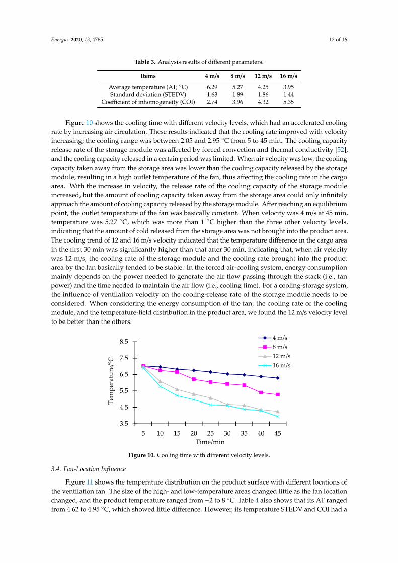
Figure 10 shows the cooling time with different velocity levels, which had an accelerated coolingrate by increasing air circulation. These results indicated that the cooling rate improved with velocityincreasing; the cooling range was between 2.05 and 2.95 ◦C from 5 to 45 min. The cooling capacityrelease rate of the storage module was affected by forced convection and thermal conductivity [52],and the cooling capacity released in a certain period was limited. When air velocity was low, the coolingcapacity taken away from the storage area was lower than the cooling capacity released by the storagemodule, resulting in a high outlet temperature of the fan, thus affecting the cooling rate in the cargoarea. With the increase in velocity, the release rate of the cooling capacity of the storage moduleincreased, but the amount of cooling capacity taken away from the storage area could only infinitelyapproach the amount of cooling capacity released by the storage module. After reaching an equilibriumpoint, the outlet temperature of the fan was basically constant. When velocity was 4 m/s at 45 min,temperature was 5.27 ◦C, which was more than 1 ◦C higher than the three other velocity levels,indicating that the amount of cold released from the storage area was not brought into the product area.The cooling trend of 12 and 16 m/s velocity indicated that the temperature difference in the cargo areain the first 30 min was significantly higher than that after 30 min, indicating that, when air velocitywas 12 m/s, the cooling rate of the storage module and the cooling rate brought into the productarea by the fan basically tended to be stable. In the forced air-cooling system, energy consumptionmainly depends on the power needed to generate the air flow passing through the stack (i.e., fanpower) and the time needed to maintain the air flow (i.e., cooling time). For a cooling-storage system,the influence of ventilation velocity on the cooling-release rate of the storage module needs to beconsidered. When considering the energy consumption of the fan, the cooling rate of the coolingmodule, and the temperature-field distribution in the product area, we found the 12 m/s velocity levelto be better than the others.

Energies 2020, 13, x FOR PEER REVIEW 12 of 16

Items 4 m/s 8 m/s 12 m/s 16 m/s Average temperature (AT; °C) 6.29 5.27 4.25 3.95 Standard deviation (STEDV) 1.63 1.89 1.86 1.44

Coefficient of inhomogeneity (COI) 2.74 3.96 4.32 5.35

Figure 10 shows the cooling time with different velocity levels, which had an accelerated cooling rate by increasing air circulation. These results indicated that the cooling rate improved with velocity increasing; the cooling range was between 2.05 and 2.95 °C from 5 to 45 min. The cooling capacity release rate of the storage module was affected by forced convection and thermal conductivity [52], and the cooling capacity released in a certain period was limited. When air velocity was low, the cooling capacity taken away from the storage area was lower than the cooling capacity released by the storage module, resulting in a high outlet temperature of the fan, thus affecting the cooling rate in the cargo area. With the increase in velocity, the release rate of the cooling capacity of the storage module increased, but the amount of cooling capacity taken away from the storage area could only infinitely approach the amount of cooling capacity released by the storage module. After reaching an equilibrium point, the outlet temperature of the fan was basically constant. When velocity was 4 m/s at 45 min, temperature was 5.27 °C, which was more than 1 °C higher than the three other velocity levels, indicating that the amount of cold released from the storage area was not brought into the product area. The cooling trend of 12 and 16 m/s velocity indicated that the temperature difference in the cargo area in the first 30 min was significantly higher than that after 30 min, indicating that, when air velocity was 12 m/s, the cooling rate of the storage module and the cooling rate brought into the product area by the fan basically tended to be stable. In the forced air-cooling system, energy consumption mainly depends on the power needed to generate the air flow passing through the stack (i.e., fan power) and the time needed to maintain the air flow (i.e., cooling time). For a cooling-storage system, the influence of ventilation velocity on the cooling-release rate of the storage module needs to be considered. When considering the energy consumption of the fan, the cooling rate of the cooling module, and the temperature-field distribution in the product area, we found the 12 m/s velocity level to be better than the others.

Figure 10. Cooling time with different velocity levels.

3.4. Fan-Location Influence

Figure 11 shows the temperature distribution on the product surface with different locations of the ventilation fan. The size of the high- and low-temperature areas changed little as the fan location changed, and the product temperature ranged from −2 to 8 °C. Table 4 also shows that its AT ranged from 4.62 to 4.95 °C, which showed little difference. However, its temperature STEDV and COI had a large difference when the fan location changed, ranging from 0.87 to 1.86 and 2.10 to 4.32, respectively. STEDV and COI results indicated that the temperature distribution in the container was more uniform when the fan was located at the top four corners of the container. The trajectory of the

3.5

4.5

5.5

6.5

7.5

8.5

5 10 15 20 25 30 35 40 45

Tem

pera

ture

/℃

Time/min

4 m/s8 m/s12 m/s16 m/s

Figure 10. Cooling time with different velocity levels.

3.4. Fan-Location Influence

Figure 11 shows the temperature distribution on the product surface with different locations ofthe ventilation fan. The size of the high- and low-temperature areas changed little as the fan locationchanged, and the product temperature ranged from −2 to 8 ◦C. Table 4 also shows that its AT rangedfrom 4.62 to 4.95 ◦C, which showed little difference. However, its temperature STEDV and COI had a

Energies 2020, 13, 4765 13 of 16

large difference when the fan location changed, ranging from 0.87 to 1.86 and 2.10 to 4.32, respectively.STEDV and COI results indicated that the temperature distribution in the container was more uniformwhen the fan was located at the top four corners of the container. The trajectory of the air is longer whenthe fan was located at the top four corners of the container, so the cold air would exchange sufficientheat with the products, and resulted in more uniform temperature distribution in the container.

Energies 2020, 13, x FOR PEER REVIEW 13 of 16

air is longer when the fan was located at the top four corners of the container, so the cold air would exchange sufficient heat with the products, and resulted in more uniform temperature distribution in the container.

(a)

(b)

(c)

(d)

Figure 11. Temperature distribution with different fan locations: (a) L0; (b) L1; (c) L2; and (d) L3.

Table 4. Analysis results of different parameters.

Items L0 L1 L2 L3 Average temperature (AT; °C) 4.25 4.13 4.62 4.95 Standard deviation (STEDV) 1.86 0.87 1.51 1.49

Coefficient of inhomogeneity (COI) 4.32 2.10 3.3 2.68

4. Conclusions

This paper studied the uniformity of temperature distribution in a novel insulated temperature-controlled container (ITCC). A CFD method was adopted to simulate the flow field and heat-transfer mechanism, which provided more insightful understanding of the heat transfer in the container. Mesh size was studied for better precision before simulation, and experiment validation showed that the simulation values were in good agreement with the experiment values. Four ventilation-velocity levels and four locations of the ventilation fan were selected to compare their temperature distribution in the container. The following conclusions were drawn.

(1) Ventilation velocity had great influence on the cooling time. Cooling rate improved as velocity increased, and temperature at 45 min was lowest when velocity was 16 m/s.

(2) The coefficient of inhomogeneity increased when velocity increased, which indicated bad temperature uniformity. However, considering the energy consumption of the fan, the cooling rate of the cooling module, and the temperature-field distribution in the product area, 12 m/s velocity was better than the others.

(3) Temperature standard deviation in the container and coefficient of inhomogeneity were the lowest when the fans were located at the top four corners of the container, namely, 0.87 and 2.1, respectively. Compared with before, the average temperature in the box was decreased by 0.12 °C, and the coefficient of inhomogeneity was decreased by more than twofold.

The simulation and experiment results showed good agreement; thus, the present study can provide a reference for research on parameter optimization of insulated temperature-controlled containers. However, the results of this study cannot be generalized to any space conditions because they are relevant to the specific conditions of the experiment.

Author Contributions: Conceptualization and methodology, B.L. and X.W.; software, Y.C.; validation, Y.C. and H.S.; formal analysis, J.G.; writing—original-draft preparation, B.L.; writing—review and editing, all authors; visualization, B.L.; supervision, H.L., J.X. and E.L. All authors have read and agreed to the published version of the manuscript.

Funding: This research was funded by the National Natural Science Foundation of China, grant nos. 31971806 and 31901736; the Natural Science Foundation of Guangdong Province, grant no. 2020A1515010967; the Guangdong Provincial Agricultural Technology Innovation and Promotion Project in 2019, grant no. 2019KJ101;

Figure 11. Temperature distribution with different fan locations: (a) L0; (b) L1; (c) L2; and (d) L3.

Table 4. Analysis results of different parameters.

Items L0 L1 L2 L3

Average temperature (AT; ◦C) 4.25 4.13 4.62 4.95Standard deviation (STEDV) 1.86 0.87 1.51 1.49

Coefficient of inhomogeneity (COI) 4.32 2.10 3.3 2.68

4. Conclusions

This paper studied the uniformity of temperature distribution in a novel insulatedtemperature-controlled container (ITCC). A CFD method was adopted to simulate the flow fieldand heat-transfer mechanism, which provided more insightful understanding of the heat transferin the container. Mesh size was studied for better precision before simulation, and experimentvalidation showed that the simulation values were in good agreement with the experiment values.Four ventilation-velocity levels and four locations of the ventilation fan were selected to compare theirtemperature distribution in the container. The following conclusions were drawn.

(1) Ventilation velocity had great influence on the cooling time. Cooling rate improved as velocityincreased, and temperature at 45 min was lowest when velocity was 16 m/s.

(2) The coefficient of inhomogeneity increased when velocity increased, which indicated badtemperature uniformity. However, considering the energy consumption of the fan, the cooling rate ofthe cooling module, and the temperature-field distribution in the product area, 12 m/s velocity wasbetter than the others.

(3) Temperature standard deviation in the container and coefficient of inhomogeneity were thelowest when the fans were located at the top four corners of the container, namely, 0.87 and 2.1,respectively. Compared with before, the average temperature in the box was decreased by 0.12 ◦C,and the coefficient of inhomogeneity was decreased by more than twofold.

The simulation and experiment results showed good agreement; thus, the present study canprovide a reference for research on parameter optimization of insulated temperature-controlledcontainers. However, the results of this study cannot be generalized to any space conditions becausethey are relevant to the specific conditions of the experiment.

Author Contributions: Conceptualization and methodology, B.L. and X.W.; software, Y.C.; validation, Y.C. andH.S.; formal analysis, J.G.; writing—original-draft preparation, B.L.; writing—review and editing, all authors;visualization, B.L.; supervision, H.L., J.X. and E.L. All authors have read and agreed to the published version ofthe manuscript.

Energies 2020, 13, 4765 14 of 16

Funding: This research was funded by the National Natural Science Foundation of China, grant nos. 31971806 and31901736; the Natural Science Foundation of Guangdong Province, grant no. 2020A1515010967; the GuangdongProvincial Agricultural Technology Innovation and Promotion Project in 2019, grant no. 2019KJ101; the Researchand Development and Innovation Team of Common Key Technologies for Agricultural-Product PreservationLogistics, grant no. 2019KJ145; and the Guangdong Province Key Field R&D Program, grant no. 2019B020225001.

Acknowledgments: The authors are grateful for the support of the South China Agricultural University andGuangzhou Hicool Technology Co., Ltd. The authors also thank the anonymous reviewers for their criticalcomments and suggestions to improve the manuscript.

Conflicts of Interest: The authors declare no conflict of interest.

References

1. Liu, M.; Saman, W.; Bruno, F. Computer simulation with TRNSYS for a mobile refrigeration systemincorporating a phase change thermal storage unit. Appl. Energy 2014, 132, 226–235. [CrossRef]

2. Mercier, S.; Villeneuve, S.; Mondor, M.; Uysal, I. Time-Temperature Management along the Food Cold Chain:A Review of Recent Developments. Compr. Rev. Food Sci. Food Saf. 2017, 16, 647–667. [CrossRef]

3. Oury, A.; Namy, P.; Youbi-Idrisi, M. Aero-thermal Simulation of a Refrigerated Truck under Open/Closed-DoorCycles. In Proceedings of the 2015 COMSOL Conference, Grenoble, France, 14 November 2015.

4. Liu, M.; Saman, W.; Bruno, F. Development of a novel refrigeration system for refrigerated trucks incorporatingphase change material. Appl. Energy 2012, 92, 336–342. [CrossRef]

5. Ahmed, M.; Meade, O.; Medina, M.A. Reducing heat transfer across the insulated walls of refrigerated trucktrailers by the application of phase change materials. Energy Convers. Manag. 2010, 51, 383–392. [CrossRef]

6. Pielichowska, K.; Pielichowski, K. Phase change materials for thermal energy storage. Prog. Mater. Sci. 2014,65, 67–123. [CrossRef]

7. Zhou, D.; Zhao, C.Y.; Tian, Y. Review on thermal energy storage with phase change materials (PCMs) inbuilding applications. Appl. Energy 2012, 92, 593–605. [CrossRef]

8. Oró, E.; Miró, L.; Farid, M.M.; Cabeza, L.F. Thermal analysis of a low temperature storage unit using phasechange materials without refrigeration system. Int. J. Refrig. 2012, 35, 1709–1714. [CrossRef]

9. Liu, L.; Su, D.; Tang, Y.; Fang, G. Thermal conductivity enhancement of phase change materials for thermalenergy storage: A review. Renew. Sustain. Energy Rev. 2016, 62, 305–317. [CrossRef]

10. Fioretti, R.; Principi, P.; Copertaro, B. A refrierated container envelope with a PCM (Phase Change Material)layer: Experimental and theoretical investigation in a representative town in Central Italy. Energy Convers.Manag. 2016, 122, 131–141. [CrossRef]

11. Oró, E.; de Gracia, A.; Cabeza, L.F. Active phase change material package for thermal protection of ice creamcontainers. Int. J. Refrig. 2013, 36, 102–109. [CrossRef]

12. Wang, C.; He, Z.; Li, H.; Wennerstern, R.; Sun, Q. Evaluation on Performance of a Phase Change MaterialBased Cold Storage House. Energy Procedia 2017, 105, 3947–3952. [CrossRef]

13. Yusufoglu, Y.; Apaydin, T.; Yilmaz, S.; Paksoy, H.O. Improving performance of household refrigerators byincorporating phase change materials. Int. J. Refrig. 2015, 57, 173–185. [CrossRef]

14. Huang, L.; Piontek, U. Improving Performance of Cold-Chain Insulated Container with Phase ChangeMaterial: An Experimental Investigation. Appl. Sci. 2017, 7, 1288. [CrossRef]

15. Gin, B.; Farid, M.M. The use of PCM panels to improve storage condition of frozen food. J. Food Eng. 2010,100, 372–376. [CrossRef]

16. Liu, G.; Wu, J.; Alan, F.; Xie, R.; Tang, H.; Zou, Y.; Qu, R. Design and no-load performance test of GU-PCM2temperature controlled phase change storage refrigerator. Trans. Chin. Soc. Agric. Eng. 2019, 35, 288–295.

17. Xu, X.F.; Zhang, X.L.; Munyalo, J.M. Simulation Study on Temperature Field and Cold Plate Melting of ColdStorage Refrigerator Car. Energy Procedia 2017, 142, 3394–3400.

18. Zhang, Z.; Guo, Y.G.; Tian, J.J.; Li, M. Numerical simulation and experiment of temperature field distributionin box of cold plate refrigerated truck. Trans. Chin. Soc. Agric. Eng. 2013, 29, 18–24.

19. Zou, Q.; Opara, L.U.; McKibbin, R. A CFD modeling system for airflow and heat transfer in ventilatedpackaging for fresh foods: I. Initial analysis and development of mathematical models. J. Food Eng. 2006, 77,1037–1047. [CrossRef]

20. Jiang, T.; Xu, N.; Luo, B.; Deng, L.; Wang, S.; Gao, Q.; Zhang, Y. Analysis of an internal structure for refrigeratedcontainer: Improving distribution of cooling capacity. Int. J. Refrig. 2020, 113, 228–238. [CrossRef]

Energies 2020, 13, 4765 15 of 16

21. Jedermann, R.; Geyer, M.; Praeger, U.; Lang, W. Sea transport of bananas in containers–Parameter identificationfor a temperature model. J. Food Eng. 2013, 115, 330–338. [CrossRef]

22. Delele, M.A.; Ngcobo, M.E.K.; Getahun, S.T.; Chen, L.; Mellmann, J.; Opara, U.L. Studying airflow and heattransfer characteristics of a horticultural produce packaging system using a 3-D CFD model. Part II: Effect ofpackage design. Postharvest Biol. Technol. 2013, 86, 546–555. [CrossRef]

23. Zhang, Z.; Li, L.; Tian, J.; Guo, Y.; Li, Y. Effects of refrigerated truck temperature field uniformity onpreservation of vegetables. Trans. Chin. Soc. Agric. Eng. 2014, 30, 309–316.

24. Defraeye, T.; Nicolai, B.; Kirkman, W.; Moore, S.; Niekerk, S.V.; Verboven, P.; Cronjé, P. Integral performanceevaluation of the fresh-produce cold chain: A case study for ambient loading of citrus in refrigeratedcontainers. Postharvest Biol. Technol. 2016, 112, 1–13. [CrossRef]

25. Trias, F.X.; Oliet, C.; Rigola, J.; Pérez-Segarra, C.D. A simple optimization approach for the insulationthickness distribution in household refrigerators. Int. J. Refrig. 2018, 93, 169–175. [CrossRef]

26. Thiessen, S.; Knabben, F.T.; Melo, C.; Gonçalves, J.M. A study on the effectiveness of applying vacuuminsulation panels in domestic refrigerators. Int. J. Refrig. 2018, 96, 10–16. [CrossRef]

27. Hammond, E.C.; Evans, J.A. Application of Vacuum Insulation Panels in the cold chain–Analysis of viability.Int. J. Refrig. 2014, 47, 58–65. [CrossRef]

28. Smale, N.J.; Moureh, J.; Cortella, G. A review of numerical models of airflow in refrigerated food applications.Int. J. Refrig. 2006, 29, 911–930. [CrossRef]

29. Sajadiye, S.M.; Zolfaghari, M. Simulation of in-line versus staggered arrays of vented pallet boxes forassessing cooling performance of orange in cool storage. Appl. Therm. Eng. 2017, 115, 337–349. [CrossRef]

30. Moureh, J.; Flick, D. Airflow pattern and temperature distribution in a typical refrigerated truck configurationloaded with pallets. Int. J. Refrig. 2004, 27, 464–474. [CrossRef]

31. Kayansayan, N.; Alptekin, E.; Ezan, M.A. Thermal analysis of airflow inside a refrigerated container. Int. J.Refrig. 2017, 84, 76–91. [CrossRef]

32. Jara, P.B.T.; Rivera, J.J.A.; Merino, C.E.B.; Silva, E.V.; Farfán, G.A. Thermal behavior of a refrigerated vehicle:Process simulation. Int. J. Refrig. 2019, 100, 124–130. [CrossRef]

33. Han, J.; Zhu, W.; Ji, Z. Comparison of veracity and application of different CFD turbulence models forrefrigerated transport. Artif. Intell. Agric. 2019, 3, 11–17.

34. Yang, T.; Wang, C.; Sun, Q.; Wennersten, R. Study on the application of latent heat cold storage in a refrigeratedwarehouse. Energy Procedia 2017, 142, 3546–3552. [CrossRef]

35. Xie, R.; Tang, H.; Tao, W.; Liu, G.; Liu, J.; Wu, J. Optimization of cold-plate location in refrigerated vehiclesbased on simulation and test of no-load temperature field. Trans. Chin. Soc. Agric. Eng. 2017, 33, 290–298.

36. Guo, J.; Fang, S.; Zeng, Z.; Lu, H.; Lü, E. Numerical simulation and experimental verification on humidityfield for pipeline humidifying device. Trans. Chin. Soc. Agric. Eng. 2015, 31, 57–64.

37. Cheng, W.; Yuan, X. Numerical analysis of a novel household refrigerator with shape-stabilized PCM (phasechange material) heat storage condensers. Energy 2013, 59, 265–276. [CrossRef]

38. Chourasia, M.K.; Goswami, T.K. Simulation of Effect of Stack Dimensions and Stacking Arrangement onCool-down Characteristics of Potato in a Cold Store by Computational Fluid Dynamics. Bioprocess Eng. 2007,96, 503–515. [CrossRef]

39. Clarke, H.; Martinez-Herasme, A.; Crookes, R.; Wen, D.S. Experimental study of jet structure andpressurisation upon liquid nitrogen injection into water. Int. J. Multiph. Flow 2010, 36, 940–949. [CrossRef]

40. Ho, S.H.; Rosario, L.; Rahman, M.M. Numerical simulation of temperature and velocity in a refrigeratedwarehouse. Int. J. Refrig. 2010, 33, 1015–1025. [CrossRef]

41. Choi, S.; Burgess, G. Practical mathematical model to predict the performance of insulating packages.Packag. Technol. Sci. 2007, 20, 369–380. [CrossRef]

42. Fang, G.Y.; LI, H. Automobile Air Conditioning Technology, 1st ed.; China Machine Press: Beijing, China, 2002;pp. 88–89.

43. Wang, D.B.; Song, Q.W. Optimum design insulated body of refrigerated van. J. Jiangsu Ins. Technol. 1993, 14,13–18.

44. Guo, J.; Lü, E.; Lu, H.; Wang, Y.; Zhao, J. Numerical Simulation of Gas Exchange in Fresh-keeping TransportationContainers with a Controlled Atmosphere. Food Sci. Technol. Res. 2016, 22, 429–441. [CrossRef]

45. Hahn, M.; Drikakis, D. Large-eddy simulation of compressible turbulence using high-resolution methods.Int. J. Numer. Methods Fluids 2005, 47, 971–977. [CrossRef]

Energies 2020, 13, 4765 16 of 16

46. Tsoutsanis, P.; Antoniadis, A.F.; Drikakis, D. WENO schemes on arbitrary unstructured meshes for laminar,transitional and turbulent flow. J. Comput. Phys. 2014, 256, 254–276. [CrossRef]

47. Thornber, B.J.R.; Drikakis, D. Numerical dissipation of upwind schemes in low Mach flow. Int. J. Numer.Methods Fluids 2008, 56, 1535–1541. [CrossRef]

48. Söylemez, E.; Alpman, E.; Onat, A.; Yükselentürk, Y.; Hartomacıoglu, S. Numerical (CFD) and experimentalanalysis of hybrid household refrigerator including thermoelectric and vapour compression cooling systems.Int. J. Refrig. 2019, 99, 300–315. [CrossRef]

49. Aslam Bhutta, M.M.; Hayat, N.; Bashir, M.H.; Khan, A.R.; Ahmad, K.N.; Khan, S. CFD applications in variousheat exchangers design: A review. Appl. Therm. Eng. 2012, 32, 1–12. [CrossRef]

50. Jaramillo, J.E.; Pérez-Segarra, C.; Oliva, A.; Claramunt, K. Analysis of different RANS models applied toturbulent forced convection. Int. J. Heat Mass Transfer. 2007, 50, 3749–3766. [CrossRef]

51. Ambaw, A.; Bessemans, N.; Gruyters, W.; Gwanpua, S.G.; Schenk, A.; De Roeck, A.; Delele, M.A.; Verboven, P.;Nicolai, B.M. Analysis of the spatiotemporal temperature fluctuations inside an apple cool store in responseto energy use concerns. Int. J. Refrig. 2016, 66, 156–168. [CrossRef]

52. Alzuwaid, F.A.; Ge, Y.T.; Tassou, S.A.; Sun, J. The novel use of phase change materials in an open typerefrigerated display cabinet: A theoretical investigation. Appl. Energy 2016, 180, 76–85. [CrossRef]

© 2020 by the authors. Licensee MDPI, Basel, Switzerland. This article is an open accessarticle distributed under the terms and conditions of the Creative Commons Attribution(CC BY) license (http://creativecommons.org/licenses/by/4.0/).