telonic fixed frequency filters - test equipment · pdf fileseries tsa — smallest...

TELONIC FIXED FREQUENCY FILTERSENG INEERS’ D ES IGN HANDBOOK

TABLE OF CONTENTS

Introduction . . . . . . . . . . . . . . . . . . . . . . . . . . . . . . . . . . . . . . . . . . . .1Aids to use of this Catalog . . . . . . . . . . . . . . . . . . . . . . . . . . . . . . . . .2Ordering Information . . . . . . . . . . . . . . . . . . . . . . . . . . . . . . . . . . . . .3Filter Selection Guide . . . . . . . . . . . . . . . . . . . . . . . . . . . . . . . . . . .4-5Frequency and Bandwidth Tolerance Curves . . . . . . . . . . . . . . . . . . . .6Passband Relationships . . . . . . . . . . . . . . . . . . . . . . . . . . . . . . . . . . .7Passband Relationship Curves . . . . . . . . . . . . . . . . . . . . . . . . . . . . . . .8

FiltersLow Pass, Tubular . . . . . . . . . . . . . . . . . . . . . . . . . . . . . . . .9-11Bandpass, Tubular . . . . . . . . . . . . . . . . . . . . . . . . . . . . . . .12-15Highpass . . . . . . . . . . . . . . . . . . . . . . . . . . . . . . . . . . . . . .16-17Bandpass, Cavity . . . . . . . . . . . . . . . . . . . . . . . . . . . . . . . .18-21Bandpass, Interdigital . . . . . . . . . . . . . . . . . . . . . . . . . . . . .22-23Bandpass, Combline . . . . . . . . . . . . . . . . . . . . . . . . . . . . .24-25Bandpass, Miniature . . . . . . . . . . . . . . . . . . . . . . . . . . . . .26-28

FILTER INDEX BY SERIES

TBA . . . . . . . . . . . . . . .12 TLP . . . . . . . . . . . . . . . . .9TBC . . . . . . . . . . . . . . .12 TSA . . . . . . . . . . . . . . .26TBP . . . . . . . . . . . . . . .12 TSC . . . . . . . . . . . . . . .26TCA . . . . . . . . . . . . . .19 TSJ . . . . . . . . . . . . . . . .24TCB . . . . . . . . . . . . . . .19 TSF . . . . . . . . . . . . . . . .18TCC . . . . . . . . . . . . . . .19TCF . . . . . . . . . . . . . . .18TCG . . . . . . . . . . . . . .19TCH . . . . . . . . . . . . . .19THP . . . . . . . . . . . . . . .16TIF . . . . . . . . . . . . . . . .22TLA . . . . . . . . . . . . . . . .9TLC . . . . . . . . . . . . . . . .9

TELONIC BERKELEY FIXED FREQUENCY FILTERS

A world leading manufacturer of RF andmicrowave components, Telonic Berkeley has a uniqueapproach in the manufacture of filters: To offer anunlimited number of filter models in the widest selectionof filter types, that can be ordered easily by the cus-tomer. As an example, this catalog contains over 20types of filters from 10 MHz to 12GHz. Complementingthis impressive array of filter types is the most completeassortment of GUARANTEED electrical and mechanicaldesign data ever published.

GUARANTEED Filter Design and Specifying Data –These conservative and comprehensive performancedata include the effects of time, temperature, shockand vibration, and – for the first time – permit you toestablish guaranteed performance specifications forcustom filters in the field.

Attenuation Curves

Insertion Loss Curves

Passband Relationship Curves

Frequency and Bandwidth Tolerance Curves

Filter Length Curves

Outline Drawings

LOW PASS FILTERS

Tubular

Lumped Element

Stripline

HIGH PASS FILTERS

BANDPASS FILTERS

Tubular

Lumped Element

Hi Q Cavity

Helical Resonators

Interdigital

Combline

Telonic Berkeley also manufactures a broad line oftunable filters. For complete information, contact ourCustomer Service Department and request theTunable Filters Catalog.

1

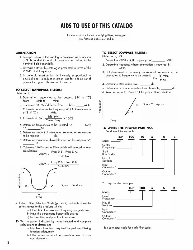
ORIENTATION1. Bandpass data in this catalog is presented as a function

of 3 dB bandwidths and all curves are normalized to thenominal 3 dB bandwidth.

2. Lowpass data in this catalog is presented in terms of theVSWR cutoff frequency.

3. In general, insertion loss is inversely proportional to physical size. To reduce insertion loss for a fixed set ofparameters, generally size must increase.

TO SELECT BANDPASS FILTERS:(Refer to Fig. 1)

1. Determine frequencies to be passed. ( ‘B’ to ‘C’ ) From ____ MHz to ____ MHz.

2. Estimate 3 dB BW if different from 1. above, _____ MHz.3. Calculate nominal center frequency ‘A’; (Arithmetic mean

of ‘B’ & ‘C’ ) ________ MHz.

4. Calculate % BW:

5. Determine frequencies to be rejected ‘D’, _______ MHz‘E’, _________ MHz.

6. Determine amount of attenuation required at frequenciesto be rejected, _________dB.

7. Determine maximum allowable insertion loss at point ‘A,’________ dB.

8. Calculate ∆ BW+ and ∆ BW – which will be used in later calculations.

9. Refer to Filter Selection Guide ( pg. 4-5 ) and write down theseries names of the products which:

a) Operate in the passband frequency range desired.b) Have the percentage bandwidth desired.c) Perform the bandpass function desired.

10. Turn to pages indicated by types selected and complete calculations to determine:

a) Number of sections required to perform filteringfunction adequately.

b) Filter series required for insertion loss or size considerations.

TO SELECT LOWPASS FILTERS:(Refer to Fig. 2 )1. Determine VSWR cutoff frequency: ‘A’ _________ MHz.2. Determine frequency where attenuation is required ‘B’

_________ MHz.3. Calculate relative frequency as ratio of frequency to be

attenuated to frequency to be passed:

4. Determine attenuation level, ________dB.5. Determine maximum insertion loss allowable, ________dB.6. Refer to pages 9, 10 and 11 for proper filter selection.

TO WRITE THE PROPER PART NO.1. Bandpass filter example

TBP 100 10 5 A BSeriesCenter Frequency3 dB BandwidthNo. of SectionsInput Connector*Output Connector*

2. Lowpass filter example

TLP 100 5 A BSeries Cutoff FrequencyNo. of SectionsInput Connector*Output Connector*

*See connector code for each filter series

AIDS TO USE OF THIS CATALOG

2

If you are not familiar with specifying filters, we suggest you first read pages 6, 7 and 8.

3dB BW —————— X 100%Center Freq.

Freq @ E – Freq @ A, ∆BW+= ——————————

3 dB BW

Freq @ A – Freq @ D, ∆BW–= ——————————

3 dB BW

Figure 1 Bandpass

Figure 2 Lowpass

‘B’ MHz R = ————

‘A’ MHz

HOW TO ORDERSignificant specifications and specific instructions should beincluded in your order whenever you desire special options orfeatures.

Filters may be ordered by (A) standard model numbers that can easily be derived by following the ordering instructionsin each filter section of this catalog or (B) by sending your specific requirements to Telonic Berkeley.

WHERE TO ORDERIn the United States and Canada your order may be placedthrough our local representative or placed directly with the factory:

TELONIC BERKELEYP.O. Box 277 Laguna Beach, California 92652

TECHNICAL DATATelonic Berkeley filters are 100% inspected to verify that all elec-trical and mechanical specifications are met. Written test datais provided on 10% of units shipped, or ten units, whichever isgreater. This test data is recorded for performance at room tem-perature only. All units are, however, exposed to temperaturesin excess of rated limits to ensure that they meet and exceedpublished specifications.

Test data covering an entire lot of filters ordered is available atan additional charge. Data recorded at temperature extremesmay also be provided at extra cost. Telonic Berkeley would bepleased to quote our customers’ specific test data requirements,and to supply such data as specified by purchase order.

TECHNICAL ASSISTANCETelonic Berkeley is represented throughout the world by a qualified staff of field engineers and representatives. They areavailable to supply you, without obligation, with technical data,literature, application engineering and assistance in selecting,specifying and ordering Telonic filters and instruments.

SHIPPING INSTRUCTIONSUnless specific instructions accompany the order we shall useour own judgment as to the best method of shipment. Unlessotherwise specified normal shipments will be by express ortruck transportation. Small items are sent via parcel post. The price for our products includes packing but does not includeshipping.

PRICES AND DELIVERYPrices for all products are published on a separate price scheduleand are in effect at the date of publication. All prices are f.o.b.factory and are subject to change without notice. Contact yournearest Telonic representative to confirm prices and obtain cur-rent delivery information. Formal price and delivery quotationsremain in effect for 30 days.

CONDITIONS AND TERMSDetermination of prices, terms, conditions of sale and finalacceptance of order are made only at Telonic, Laguna Beach,California. Terms are net 20 days and prices are f.o.b. factory.Unless credit has already been established shipments will bemade C.O.D., or on receipt of cash in advance.

MINIMUM BILLINGThe minimum billing per order is $50.00. This applies to allpurchases.

WARRANTYStandard filters manufactured by Telonic are guaranteed for aperiod of ONE YEAR from date of purchase against defectivematerials and workmanship. Telonic expressly limits its liabilityto replacement or repair of the article furnished except for tubesor batteries. This warranty does not apply to products that havebeen disassembled, modified or subjected to conditions exceedingthe applicable specifications and ratings. In the event of any ofthe foregoing, the guarantee will be void. Telonic disclaims anywarranty other than as specifically set forth herein and may discontinue models or alter their specifications without notice.

SERVICE AND PARTSRepair service and parts are available from our plant at Laguna Beach, California.

To return items for repair, please contact the Sales Departmentat the factory for permission to return. All returned goods areto be shipped prepaid and must be identified by purchaseorder number, model number, serial number and nature of malfunction.

ORDERING INFORMATION

3

OUR TOLL FREE LINE800-854-2436

SECTION 1. TUBULAR LOW/PASS FILTERS

SECTION 2. TUBULAR BANDPASS FILTERS

SECTION 3. HIGHPASS FILTERS

SECTION 4. CAVITY BANDPASS FILTERS

SECTION 5. INTERDIGITAL BANDPASS FILTERS

SECTION 6. COMBLINE BANDPASS FILTERS

SECTION 7. MINIATURE BANDPASS FILTERS

4

FILTER SELECTION GUIDE

BANDWIDTH

Series TLP — Lumped constant, 1/2“ diam., low cost, small size —Series TLA — Lumped constant, 3/4” diam., intermediate loss, size, power —Series TLC — Lumped constant, 1 1/4” diam., low loss, highest power —

Series TBP — Lumped constant, 1/2“ diam., lowest cost, most popular 2 – 30% Series TBA — Lumped constant, 3/4“ diam., medium loss and power 2 – 30% Series TBC — Lumped constant, 1 1/4” diam., lowest loss, highest power 2 – 30%

Series TSA — Smallest available helical filter, P.C.B. mounting available 1 – 15%Series TSC — Intermediate size helical, P.C.B. mounting available 1 – 15%

Series TSF — Lowest loss helical resonator series 1 – 3%Series TCF — Quarter-wavelength, coaxial, modular slotted box construction .3 – 3%Series TCC — Quarter-wavelength, coaxial, lowest loss, re-entrant cavity .3 – 3%Series TCA — Quarter-wavelength, coaxial, ideal size vs. performance parameters for general cavity filter req. .3 – 3%Series TCG — Quarter-wavelength, coaxial, highest frequency, re-entrant cavity .3 – 2%Series TCH — TM-010 mode extremely narrow band .1 – 1%Series TCB — Adjustable quarter-wavelength, coaxial, up to 10% tuning range .3 – 3%

Series THP — Distributed constant, small size, low loss —

Series T IF — Strip line, air dielectric 3 – 30%

Series TSJ — Miniature combline filters utilizing air dielectric 1 – 15%

5

F R E Q U E N C Y R A N G E * PAGE20 MHz 50 MHz 100 MHz 200 MHz 500 MHz 1GHz 2 GHz 5 GHz 10 GHz

* Gray areas indicate special extended ranges.

999

121212

16

18181818181818

22

24

2626

6

FREQUENCY AND BANDWIDTH TOLERANCE CURVES

FREQUENCY AND BANDWIDTH

A DISCUSSION OF FREQUENCY AND BANDWIDTH TOLERANCES AS THEYAPPLY TO FILTERS MANUFACTURED BY TELONIC.Figures 1 and 2 illustrate the standard specification format forlowpass and bandpass filters. The shaded areas represent specification limits which apply under all operating conditionsdefined in the filter specifications.

A plot of the filter performance will always lie outside of theshaded areas.

Figures 3 and 4 show the plot of a typical filter superimposedon the same specification limits.

Each filter built to the same specifications may be slightly different, but will meet or exceed the electrical specificationswhile being exposed to the specified operating environmentalconditions.

Should a requirement arise for a unit with a specific bandwidthtolerance, submit all of your requirements (mechanical, environmental, and electrical ) to the factory. This will assure theoptimal design to meet your needs.

Figure 1. Lowpass Filter Performance Limits.

Figure 2. Bandpass Filter Performance Limits.

Figure 3. Typical Lowpass Filter Curve.

Figure 4. Typical Bandpass Filter Curve.

7

PASSBAND RELATIONSHIPS

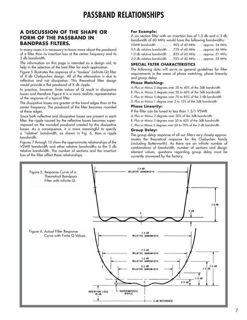
Figure 5. Response Curve of aTheoretical BandpassFilter with Infinite Q.

Figure 6. Actual Filter Response Curve with Finite Q Values.

A DISCUSSION OF THE SHAPE ORFORM OF THE PASSBAND IN BANDPASS FILTERS.In many cases it is necessary to know more about the passbandof a filter than its insertion loss at the center frequency and its 3 db bandwidth.The information on this page is intended as a design aid, tohelp in the selection of the best filter for each application. Figure 5 illustrates the response of a “lossless” (infinite Q) filterof X db Chebyschev design. All of the attenuation is due toreflection and not dissipation. This theoretical filter designwould provide a flat passband of X db ripple.In practice, however, finite values of Q result in dissipative losses and therefore Figure 6 is a more realistic representationof the response of a typical filter.The dissipative losses are greater at the band edges than at thecenter frequency. The passband of the filter becomes roundedat these edges. Since both reflective and dissipative losses are present in eachfilter, the ripple caused by the reflective losses becomes super-imposed on the rounded passband created by the dissipativelosses. As a consequence, it is more meaningful to specify a “relative” bandwidth, as shown in Fig. 6, than a ripple bandwidth.Figures 7 through 10 show the approximate relationships of theVSWR bandwidth and other relative bandwidths to the 3 db relative bandwidth. The number of sections and the insertionloss of the filter affect these relationships.

For Example:A six section filter with an insertion loss of 1.5 db and a 3 dbbandwidth of 60 MHz would have the following bandwidths:VSWR bandwidth . . . . . . . . .90% of 60 MHz . . . .approx. 54 MHz0.5 db relative bandwidth . . .73% of 60 MHz . . . .approx. 44 MHz1.0 db relative bandwidth . . .85% of 60 MHz . . . .approx. 51 MHz2.0 db relative bandwidth . . .92% of 60 MHz . . . .approx. 55 MHz

SPECIAL FILTER CHARACTERISTICSThe following data will serve as general guidelines for filterrequirements in the areas of phase matching, phase linearityand group delay. Phase Matching:A.Plus or Minus 2 degrees over 30 to 40% of the 3dB bandwidthB. Plus or Minus 3 degrees over 50 to 60% of the 3dB bandwidthC. Plus or Minus 5 degrees over 70 to 85% of the 3 dB bandwidthD. Plus or Minus 1 degree over 5 to 15% of the 3dB bandwidth

Phase Linearity:If the filter can be tuned to less than 1.3/1 VSWRA.Plus or Minus 2 degrees over 30% of the 3dB bandwidthB. Plus or Minus 3 degrees over 50 to 60% of the 3dB bandwidthC. Plus or Minus 5 degrees over 60 to 70% of the 3 dB bandwidth

Group Delay:The group delay response of all our filters very closely approx-imates the theoretical response for the Chebychev family(including Butterworth). As there are an infinite number of combinations of bandwidth, number of sections and design element values, questions regarding group delay must be currently answered by the factory.

8

PASSBAND RELATIONSHIP CURVES

Figure 7. VSWR Bandwidth.

Figure 9. 1.0 dB Relative Bandwidth. Figure 10. 2.0 dB Relative Bandwidth

Figure 8. 0.5 dB Relative Bandwidth.

9

TUBULAR LOWPASS FILTERS

DESCRIPTIONAll Lowpass Series are typically of 0.1 db Chebyschev Designand are available with 2 thru 12 sections and practically anyavailable RF connector (see pages 16, 17). Special designs areavailable on request.

The specifications for the example shown here are as follows:1/2” diameter Lowpass Filter, VSWR cutoff frequency = 1600MHz, 5 sections, TNC female conn.

SPECIFICATIONSELECTRICAL SPECIFICATIONS

ENVIRONMENTAL SPECIFICATIONS

MECHANICAL SPECIFICATIONS

Cutoff Frequency Range

Stop Band Attenuation

Number of Sections

Shock

Vibration

Humidity

Altitude

Temp. Range

Temp. Range

Diameter

Approx. Weight

Shock

Vibration

OPE

RA

TIN

G

ST

ORA

GE

Average Input Power (watts max. to 10,000 ft.)

Input Peak Power (watts max. to 10,000 ft.)

Maximum Insertion Loss In Passband

Nominal Impedance (in and out)

Maximum VSWR In Passband

Normal Spec. Limit

Normal Spec. Limit

Normal Spec. Limit

Normal Spec. Limit

Normal Spec. Limit

Normal Spec. Limit

Normal Spec. Limit

Normal Spec. Limit

Normal Spec. Limit

Normal Spec. Limit

Normal Spec. Limit

Normal Spec. Limit

Normal Spec. Limit

Normal Spec. Limit

Normal Spec. Limit

Normal Spec. Limit

*Areas of Interest

*Areas of Interest

*Areas of Interest

*Areas of Interest

*Areas of Interest

*Areas of Interest

*Areas of Interest

*Areas of Interest

*Areas of Interest

*Areas of Interest

*Areas of Interest

*Areas of Interest

*Areas of Interest

*Areas of Interest

*Areas of Interest

100 MHz to 2750 MHz ( See Note 1 )

As Low as 60 MHz See Graph

Submit Requirements

50 ohms

1.5:1 As Low As 1.2:1

See Page11 Submit Requirements

2 to 8 2 to 12

500

10,000

30G

30G

10G

10G100G

1/2 inch3/4 oz. per inch

50G

Up to 90%

Unlimited-20˚C to +50˚C-54˚C to +125˚C

– 54˚C to + 71˚C– 62˚C to +150˚C

To 100% with Condensation

1000G

1000G

5Loss Constant

12Loss Constant

50 to 100 ohms

TLP



Submit Requirements

50 ohms

1.5:1 As Low As 1.2:1


2 to 8 2 to 12

500

10,000

15G

15G

5G

5G30G


30G

Up to 90%


– 54˚C to + 71˚C– 62˚C to +150˚C


75G

75G

8Loss Constant

20Loss Constant

50 to 100 ohms

TLA



Submit Requirements

50 ohms

1.5:1 As Low As 1.2:1


3 to 6 2 to 12

1000

10,000

15G

15G

5G

5G30G

11/4 inch

11/4 oz. per inch

30G

Up to 90%


– 54˚C to + 71˚C– 62˚C to +150˚C


75G

75G

15Loss Constant

40Loss Constant

50 to 100 ohms

TLC

SERIES TLP100 to 2,750 MHz

1/2” diam.low cost

small size

SERIES TLA50 to 1,500 MHz

3/4” diam.intermediate loss

size power

SERIES TLC30 to 1,000 MHz

11/4” diam.low loss

highest power

* A — BNC Jack* B — BNC Plug

C — TNC JackD — TNC PlugE — N JackF — N PlugS — SMA JackT — SMA PlugX — Special

* BNC Connectors not standard above 1000 MHz

NOTE 1: See page 6 for standard tolerance on cutoff frequency. The normal specification passband is from 0.4 x cutoff frequency to cutoff. A wider specification pass-band can be supplied. Telonic will be happy to advise on all such special requirements.

*Submit specific requirements

TLP 1600 — 5 C C

Series

Nominal Cutoff Frequency in MHz

Number of Sections

See Connector Input Conn.Code, Below Output Conn.

Suffix Number to be Assigned by the Factory to Identify the Specific Customer and Application

{

30 TO 2,750 MHz 2 TO 12 SECTIONS

SECTION 1

CO

NN

ECTO

R C

OD

E

10

TUBULAR LOWPASS FILTERS ATTENUATION CURVES

The curves above define the normal specification limits on attenuationfor Telonic lowpass filters. The minimum attenuation level in db is shownas a function of the relative frequency.*Calculate relative frequency as ratio of frequency to be attenuated to frequency to be passed:

For example:Requirements—

1. Min. cutoff frequency = 1,600 MHz.2. 35 db min. attenuation at 2,080 MHz.

1,600 MHz is within the standard frequency ranges of two differentlowpass types — TLP and TLR. 2,080 MHz is at a relative frequency of1.3 with respect to 1600 MHz.

Reading from the 4-sec. curve (note ref. line ) at a relative frequency of1.3, we find that a four section TLP has a normal specification limit of29 db and a five section TLP has a normal specification limit of 42 db.Therefore a TLP of five or more sections would be required to meet the35 db attenuation specification. ‘B’ MHz

R = ————‘A’ MHz

2080———— = 1.31600

ABSOLUTE ATTENUATION ★ GUARANTEED SPECIFICATIONS TO 5X CUTOFF FREQUENCY

★ GUARANTEED SPECIFICATIONS

INSERTION LOSS CURVES

INSERTION LOSS:Loss = KN + .05

Where: K = Loss constantN = Number of sections

The insertion loss graph defines theloss constant which must be used tocalculate the insertion loss specification.In addition, it illustrates the relativeinsertion loss and frequency ranges of the standard Telonic lowpass filters.

For example:A five section filter with a cutoff frequency of 1,600 MHz is availablein a TLP or a TLR configuration. In accordance with the formula above,the maximum insertion loss specifica-tions are as follows.TLP 1600 – 5CC:KN + .05 = .15 X 5 + .05 = .8 dbTLR 1600 – 5CC:KN + .05 = .09 X 5 + .05 = .5 db

11

LENGTH CURVES TUBULAR LOWPASS FILTERS

LENGTH OF LOWPASS FILTERS:The approximate length of any Telonic lowpass filter can be readdirectly from these graphs. Select the graph which represents the correct series of filter. On thefrequency scale, locate the proper value of cut - off frequency.Read straight up to the length-curve line which corresponds to theproper number of sections. Then, from the point where the cutofffrequency and section line cross, read horizontally to get the properfilter length, in inches. For example:The approximate length of TLP 1600-5CC is 4.0 inches. Noteexample reading shown flagged on the TLP length curve. All of the length information shown here is approximate. Exactlength specifications must be quoted by the factory. In most casesa filter can be constructed shorter than the length shown here, butthis may cause an increase in insertion loss. If a shorter unit or onewith a specific length is needed, please submit all of your require-ments — both electrical and mechanical. This will enable Telonicto quote the optimum design for your application.

12

TUBULAR BANDPASS FILTERS

DESCRIPTIONTelonic Tubular Bandpass Filters are of 0.1 db Chebyschev design andare available with from 2 to 12 sections.Three different sizes and frequency ranges allow for the selection of an optimal design for each requirement. Almost any type of input oroutput connection is available as a standard item.The specifications for example shown here are as follows: 1/2” diam-eter Bandpass Filter with center frequency at 500 MHz 3 db BW of 50 MHz minimum, 5 pole attenuation response as defined in curves onpage 13, connector type is TNC female.

ELECTRICAL SPECIFICATIONS





Other Relative Bandwidths

Number of Sections

Shock

Vibration

Humidity

Altitude

Temp. Range

Temp. Range

Diameter

Approx. Weight

Shock

Vibration

OPE

RA

TIN

G

ST

ORA

GE


Peak Input Power (watts max. to 10,000 ft.)

Minimum 3 db Relative Bandwidth (in % of center frequency)


Maximum VSWR at Center Frequency

Minimum VSWR Bandwidth

Normal Spec. Limit

Normal Spec. Limit

Normal Spec. Limit

Normal Spec. Limit

Normal Spec. Limit

Normal Spec. Limit

Normal Spec. Limit

Normal Spec. Limit

Normal Spec. Limit

Normal Spec. Limit

Normal Spec. Limit

Normal Spec. Limit

Normal Spec. Limit

Normal Spec. Limit

Normal Spec. Limit

Normal Spec. Limit

*Areas of Interest

*Areas of Interest

*Areas of Interest

*Areas of Interest

*Areas of InterestNormal Spec. Limit *Areas of Interest

*Areas of Interest

*Areas of Interest

*Areas of Interest

*Areas of Interest

*Areas of Interest

*Areas of Interest

*Areas of Interest

*Areas of Interest

*Areas of Interest

*Areas of Interest


60 MHz to 2700 MHz

2% to 30% ( See Note 1 )

1.5% to 70%

Spl. Requirements ( See page 7 )

50 ohms

1.5:1 As Low As 1.2:1

See Page 15 Spl. Requirements ( See page 7 )

See Page 13 Spl. Requirements

2 to 6

10 KW

30G

30G

10G

10G100G


50G

Up to 90%

Unlimited0˚C to + 50˚C

–54˚C to + 125˚C

– 54˚C to + 55˚C– 62˚C to +150˚C

up to 100% with Condensation

1000G

1000G

2 to 12

50 to 100 ohms

TBP

Fc MHz

( Loss Constant ) Fc MHz)

200 ( 3 dB bw MHz )

300 ( 3 dB bw MHz )

Below500 MHz

Fc MHz600 ( 3 dB bw MHz )Above

500 MHz


35 MHz to 1500 MHz

2% to 30% ( See Note 1 )

1.5% to 70%


50 ohms

1.5:1 As Low As 1.2:1



2 to 6

10 KW

15G

15G

5G

5G30G


30G

Up to 90%


–54˚C to + 125˚C

– 54˚C to + 55˚C– 62˚C to +150˚C


75G

75G

2 to 12

50 to 100 ohms

TBA

Fc MHz


200 ( 3 dB bw MHz )

500 ( 3 dB bw MHz )

Below300 MHz


300 MHz



2% to 30% ( See Note 1 )

1.5% to 70%


50 ohms

1.5:1 As Low As 1.2:1



2 to 6

50 KW

15G

15G

5G

5G30G

11/4 inch

11/4 oz. per inch

30G

Up to 90%


–54˚C to + 125˚C

– 54˚C to + 55˚C– 62˚C to +150˚C


75G

75G

2 to 12

50 to 100 ohms

TBC

Fc MHz


400 ( 3 dB bw MHz )

1000 ( 3 dB bw MHz )

Below200 MHz


200 MHz

* A — BNC Jack* B — BNC Plug

C — TNC JackD — TNC PlugE — N JackF — N PlugS — SMA JackT — SMA PlugX — Special


NOTE 1: See page 6 for standard tolerance and definition of center frequency and bandwidth.

TBP 500 — 50 — 5 C C

Series

Nominal Center Freq. in MHz

Minimum 3 db Relative Bandwidth in MHz

Number of Sections



{

30 TO 2,400 MHz 2 TO 30% BANDWIDTH 2 TO 12 SECTIONS

SECTION 2

CO

NN

ECTO

R C

OD

E

SERIES TBP100 to 2,400 MHz

1/2” inch diam.lowest cost

most popular

SERIES TBA50 to 1,000 MHz3/4” inch diam.

medium lossand power

SERIES TBC30 to 900 MHz

11/4” inch diam.lowest loss

highest power

13

STOP BAND ATTENUATION:

These graphs show the minimum stop band attenuation in db for all three seriesof Telonic Tubular Bandpass Filters. Since the filter characteristics and productiontolerances vary for differing bandwidths, it is necessary to establish differing specifications for each bandwidth of filter. Intermediate values may be interpolated. In each case the rejection frequency is plotted in “3 db bandwidths from centerfrequency.” The exact relationships are as follows:

Any one of the following parameters may be identified if the other three and the center frequency are known.(1) Min. 3 db bandwidth ( in MHz) (2) Number of Sections(3) Rejection Frequency ( in MHz ) (4) Attenuation Level ( in db )Always verify that the frequency and bandwidth you have selected are within the limitations shown for that series of filter.Example 1: ( See page 14, 10% curve ).Given:Center frequency = 500 MHzMinimum 3 db BW = 50 MHzNumber of sections = 5Find: Minimum attenuation levels at 580 MHz and 425 MHz

Since the 3 db bandwidth is exactly 10 % of the center frequency, the answer canbe read directly from the graph marked 10% bandwidth. Using the 5-section curve and the point +1.60 (580 MHz) we find the min. atten-uation level is 50 db. At –1.50 ( 425 MHz ) the minimum attenuation level is 40 db.Example 2:

Given:Center frequency = 300 MHzNumber of sections = 3Atten. at 336 MHz = 40 db min.Find: The 3 db bandwidth

From ( II ) above—

Since we do not know the exact bandwidth we must estimate it and solve by aniterative process. All of the 3 section curves show the high frequency 40 db point at between +2.5and +3.1 3 db bandwidths from center freq. If we assume 2.8 we find an approx-imate value for the 3 db BW of 36/2.8 = 13 MHz.13 MHz is approximately 4%of 300 MHz, therefore we now know that we must interpolate between the 2%and 5% bandwidth graphs. The 2% graph shows +3.1 and the 5% graph shows+2.95. We now know that +3.0 is an accurate number to use in the above equa-tion. The accurate value for the 3 db bandwidth is 36/3.0 = 12 MHz.

TUBULAR BANDPASS FILTERS ATTENUATION CURVES

★ GUARANTEED SPECIFICATIONS TO 5X CENTER FREQUENCY


Rejection freq. MHz – Fc MHz (I ) 3 db bandwidths from center freq. = ————————————––––––

Min. 3 db BW MHz or

Rejection freq. MHz – Fc MHz(II ) Min. 3 db bandwidth in MHz = ————————————–––––––

3 db BW Fc

From ( I ) above —580-500

3 db BWs from Fc = ————— = + 1.6050

425 –500and = ——————— = – 1.5050

336 – 300Min. 3 db BW = ———————

3 db BW from Fc

14

ATTENUATION CURVES TUBULAR LOWPASS FILTERS★ GUARANTEED SPECIFICATIONS TO 5X CENTER FREQUENCY



15


LENGTH CURVES TUBULAR BANDPASS FILTERSAPPROXIMATE LENGTH OF TUBULAR BANDPASS FILTERS:To determine the approximate length of Telonic Tubular Bandpass Filters, calculate the % BW and use the formulae and graphs shown here. Your answer will be the approximate overall length including type TNC female connectors. Exact length specifications must be quoted by the factory. In most cases a filter can be constructed shorter than the length shown here, but this may cause an increase in insertion loss.If a shorter unit or one with a specific length is needed, please submit all of your requirements, both electrical and mechanical. This will enable Telonic Berkeley to quote the optimal design for your application.

When using the graphs shown here, read the length constant which corresponds with the nominal center frequency and % bandwidth of your filter.Example 1: MODEL NO. TBP 500 - 50 - 5CC

Example 2: MODEL NO. TBA 300 - 12 - 3CC

TBC: Consult factory.

100 (min. 3 db BW MHz)

Nominal Fc MHz% BW =

% BW = 100 x 50500

= 10

% BW = 100 x 12

300= 4

% BW Approx. length = K ( N +3

) + 1.6

% BW Approx. length = K ( N +3

) + 2.4

= 0.68 ( 5 + 3––10

) + 1.6

= 0.68 x 5.3 + 1.6= 5.2 inches

3––4= 0.77 ( 3 + ) + 2.4

= 0.77 x 3.75 + 2.4= 5.3 inches

CENTER FREQUENCY INSERTION LOSS:

Where: K = Loss constant from graph N = Number of sections

The graph defines the loss constant which must be used to calculate insertion loss. It also illustrates the relative insertion loss and frequency ranges of standard Telonic Tubular Bandpass Filters.For example: TBP 500 - 50 - 5CC No. of sections = 5 Center freq. = 500 MHz

Loss constant = 2.2 ( Read directly from the TBP insertion loss curve at 500 MHz.)Therefore: Max. insertion loss at Fc

K (N + 0.5 )–––––––––––

% BWLOSS = + 0.2 dB

2.2 x 5.5––––––––––10

= + 0.2 = 1.4 db

100 x 50–––––––––––500

% BW = = 10

100 ( 3 db BW )——–––––––––––Nominal Fc MHz% BW =

VSWR BandwidthNO. OF SECTIONS 2 3 4 5 6 0R MORE

0.4 0.7 0.8 0.85 0.9VSWR Bandwidth—————————Min. 3 db Bandwidth

16

TELONIC HIGHPASS FILTERS

All Highpass Series are typically of 0.1 db Chebyschev Designand are available with 2 thru 10 sections. Special designs areavailable on request.





Number of Sections

Shock

Vibration

Humidity

Altitude

Temp. Range

Temp. Range

Shock

OPE

RA

TIN

G

ST

ORA

GE



Maximum Insertion Loss In Passband*


Maximum VSWR In Passband

Normal Spec. Limit Areas of Interest

100 MHz to 500 MHz 50 MHz to 1500 MHz

See Graph

50 ohms 50 to 100 ohms

1.7:1 as low as 1.3:1

Submit Requirements

See Graph Submit Requirements

3 to 7 2 to 10

20

30G

10G 50G

Vibration 10G 50G

Up to 90%

Unlimited Unlimited

-20˚C to + 50˚C -54˚C to + 125˚C

– 54˚C to +71˚C – 62˚C to +150˚C


1000G

30G 1000G

5

100

12

*All highpass filters have an upper passband limit caused by distributed effects of the individual elements. This upper limit is dependent upon both frequency and number of sections, and can vary from 2x to 7x the cutoff frequency. Consult factory for further information.

THP 350 5 C C

Series

Nominal Center Freq. MHz

Sections



{

50 TO 1500 MHz 2 TO 10 SECTIONS

SECTION 3

The curves at right define the normal specification limits on attenuation for Telonic highpass filters. The minimum attenuation level in db is shown asa function of the relative frequency.Calculate relative frequency as ratio of frequency to be attenuated to fre-quency to be passed:

For example:Requirements –

1. Min. cutoff frequency = 350 MHz.2. 35 db min. attenuation at 250 MHz.

250 MHz is at a relative frequency of .71 with respect to 350 MHz.

Reading from the 4 - sec. curve at a relative frequency of .71, we find thata four section THP has a normal specification limit of 28 db and a five section THP has a normal specification limit of 38 db. Therefore a THP offive or more sections would be required to meet the 35 db attenuation specification.

‘B’ MHz R = ————

‘A’ MHz

250R = —— = .71

350

SERIES THP

*A — BNC Jack*B — BNC PlugC — TNC JackD — TNC Plug

E — N JackF — N Plug

S — SMA JackT — SMA PlugX — Special


CONNECTOR CODE

17

HIGHPASS ATTENUATION CURVE


INSERTION LOSS:Loss = KN + .2 (in db)

Where:K = Loss constantN = Number of sections

The insertion loss graph defines theloss constant which must be used tocalculate the insertion loss specification.

For example:In accordance with the formula above,the maximum insertion loss specifica-tions are as follows.

THP 350 -5CCKN + 0.2 = .18 x 5 + .2 =1.1db

18

Telonic Cavity Bandpass Filters exhibit lower losses and narrower band-widths than Telonic Tubular Filters, as well as higher frequency ranges.For extremely high stability over the operating temperature range, mostCavity Filters can be temperature compensated. Where the normalattenuation characteristic is not appropriate, traps, or “band-reject sections” may be added for special applications.

These filters utilize helical resonators, coaxial resonators or resonant cavities. Resonant elements are subject to higher frequency spurious responses which can usually be suppressed with aTelonic Lowpass Filter, if required.






Number of Sections

Shock

Vibration

Humidity

Altitude

Temp. Range

Temp. Range

Vibration

Shock

OPE

RA

TIN

G

ST

ORA

GE






Maximum insertion loss At Center Frequency

Normal Spec. Limit

Normal Spec. Limit

Normal Spec. Limit

Normal Spec. Limit

Normal Spec. Limit

Normal Spec. Limit

Normal Spec. Limit

Normal Spec. Limit

Normal Spec. Limit

Normal Spec. Limit

Normal Spec. Limit

Normal Spec. Limit

Normal Spec. Limit

Normal Spec. Limit

Normal Spec. Limit

Normal Spec. Limit

*Areas of Interest

*Areas of Interest

*Areas of Interest

*Areas of Interest


*Areas of Interest

*Areas of Interest

*Areas of Interest

*Areas of Interest

*Areas of Interest

*Areas of Interest

*Areas of Interest

*Areas of Interest

*Areas of Interest

*Areas of Interest

*Areas of Interest

Normal Spec. Limit

*Areas of Interest

30 to 400 MHz ( See Note 1 )

20 to 600 MHz

1.0% to 3.0% ( See Note 1 )

0.2% to 3.5%

See page 20 Spl. Requirements ( See page 7 )

Spl. Requirements

20 to100

5G

15G

5G

10G20G

15G

Up to 90%

Unlimited0˚C to 50˚C

–54˚C to + 125˚C

– 54˚C to + 71˚C– 62˚C to +150˚C


15G

75G

5 to 20

50 ohms

1.5:1 1.2:1

See Table 1 Spl. Requirements ( See page 7 )

See Spl. Requirements

2 to 6up to 10

50 to 100 ohms

TSF

( Loss Constant ) ( Fc MHz )300 ( 3 dB rel. bw MHz )

( Fc MHz )

1500 ( 3 dB rel. bw MHz )

0.4 to 3.0 GHz ( See Note 1 )

0.3 to 4.0 GHz

0.3% to 3.0% ( See Note 1 )

0.2% to 3.5%


Spl. Requirements

20 to200

5G

15G

5G

10G20G

15G

Up to 90%


–54˚C to + 125˚C

– 54˚C to + 100˚C– 62˚C to +150˚C


15G

75G

10 to 100

50 ohms

1.5:1 1.2:1



2 to 6up to 10

60 ohms

TCF

See Peak 20% of Peak

( Fc MHz )



0.3% to 3.0% ( See Note 1 )

0.1% to 3.5%


Spl. Requirements

100 to1000

25G

75G

10G

30G60G

30G

Up to 90%


–54˚C to + 125˚C

– 54˚C to + 100˚C– 62˚C to +150˚C


75G

150G

100 to 1000

50 ohms

1.5:1 1.1:1



2 to 6up to 10

60 ohms

TCC

( Fc MHz )

10,000 ( 3 dB rel. bw MHz )


CAVITY BANDPASS FILTERS30 TO 12,000 MHz 0.1 TO 3.0% BANDWIDTHS

SECTION 4


SERIES TCC■ 500 to 2,500 MHz

■ Coaxial 1/4”- wavelength resonators■ Lowest insertion loss of

the cavity designs■ Bored aluminum block

SERIES TCF■ 400 to 3,000 MHz

■ Coaxial 1/4”- wavelength resonators■ Slotted aluminum box

SERIES TSF■ 30 to 400 MHz

■ Helical resonators■ Slotted aluminum box

19

The specifications for the example shown here are as follows:This model is a fixed frequency cavity bandpass filter. It has a nominalcenter frequency of 1680 MHz and a minimum 3 db relative bandwidthof 42 MHz. The maximum insertion loss at 1680 MHz is 0.47 db (see page20). The nominal input and output impedance is 50 ohms. The maximumVSWR at center frequency is 1.5:1. From Table 1, 0.8 x 42 MHz (mini-mum 3 db bandwidth) is 33.6 MHz for a VSWR of 1.5:1 or less from1663.2 MHz to 1696.8 MHz.

TCGTCA


0.8 to 4.0 GHz

0.3% to 3.0% ( See Note 1 )

0.2% to 3.5%


Spl. Requirements

45 to 300

25G

75G

10 G

30G60G

30 G

Up to 90%


–54˚C to + 125˚C

– 54˚C to + 100˚C– 62˚C to +150˚C


75G

150G

15 to 150

50 ohms

1.5:1 1.2:1



2 to 6up to 10

60 ohms

See Peak

( Fc MHz )



1.0 to 6.0 GHz

0.3% to 2.0% ( See Note 1 )

0.2% to 3.0%


Spl. Requirements

45 to 300

25G

75G

10 G

30G60G

30 G

Up to 90%


–54˚C to + 125˚C

– 54˚C to + 100˚C– 62˚C to +150˚C


75G

150G

15 to 150

50 ohms

1.5:1 to 4 GHz 2.0:1 to 6 GHz



2 to 6up to 10

See Peak

( Fc MHz )




0.1% to 1.0% ( See Note 1 )

0.1% to 2.0% ( See Note 1 )



100 to 5000

25G

75G

10 G

30G120G

60 G

Up to 90%


–54˚C to + 125˚C

– 54˚C to + 100˚C– 62˚C to +150˚C


150G

300G

5 to 200

50 ohms

2.0:1 1.5:1



2 to 41 to 8

10% of Peak

( Fc MHz )

15,000 ( 3 dB rel. bw MHz )

1.0 to 2.4 GHz Tuning Range up to 10% ( See Note 1 )

1.0 to 3.0 GHz

0.3% to 3.0% ( See Note 1 )

0.2% to 3.5%



2 to 300

5G

5G

5 G

5G15G

10 G

Up to 90%


–54˚C to + 125˚C

– 54˚C to + 100˚C– 62˚C to +150˚C


15G

25G

2 to 150

50 ohms

1.5:1


See Page 20 Similar to TCA

2 to 4

60 ohms

See Peak

( Fc MHz )

1,000 ( 3 dB rel. bw MHz )

TCH TCB

SERIES TCB■ 1.0 to 2.4 GHz

■ Coaxial 1/4”- wavelength resonators■ Adjustable center frequency

■ Bored aluminum block

SERIES TCA■ 1.0 to 3.0 GHz

■ Coaxial 1/4”- wavelength resonators■ Bored aluminum block

SERIES TCG■ 2.0 to 6.0 GHz

■ Coaxial 1/4”- wavelength resonators■ Bored aluminum block

SERIES TCH■ 6.0 to 12.0 GHz

■ TM010 resonant cavity■ Bored aluminum block

TCA 1680 — 42 — 4 E E

Series

Nominal Center Frequency

Minimum 3 db Bandwidth

Number of Sections

See page 21 for Input Conn.Connector Code Output Conn.

Suffix Number to be Assigned by the Factory to Identify the Specific Customer and Application.

{

*Submit specific requirements for quotation

20

CAVITY BANDPASS FILTERS ATTENUATION

STOP BAND ATTENUATION:This graph shows the minimum stop band attenua-tion in db for Telonic cavity bandpass filters with lessthan 3 db insertion loss. Filters with higher loss mustbe quoted by the factory. The rejection frequency is plotted in “3 db bandwidthsfrom center frequency.” The exact relationships are:( I ) 3 db bandwidths from Fc

or ( II ) Min. 3 db bandwidth in MHz

Any one of the following parameters may be identified if the other three and the center frequency are known.(1 ) Min. 3 db bandwidth (in MHz).(2 ) Number of sections.(3 ) Rejection Frequency (in MHz).(4 ) Attenuation Level (in db).

Always verify that the frequency and bandwidth you have selected are within the limitations shownfor that series of filter.

For example:Given:Center frequency = 1,680 MHzMinimum 3 db BW = 42 MHzNumber of sections = 4Find: Minimum attenuation level at 1,608 MHz and 1,752 MHz.From ( I ) above: 3 db BWs from Fc

Reading directly from the graph at the points –1.71 and+1.71 we find the minimum attenuation level of 40 db.

Rej. freq. MHz – Fc MHz= ——————————————

Min. 3 db BW MHz


3 db BWs from Fc

1608 – 1680 = —————— = –1.71

421752 – 1680

and —————— = + 1.7142

INSERTION LOSS

INSERTION LOSS:

Where: K = Loss constantN = Number of sections

The insertion loss graph defines the loss constantused to calculate the insertion loss specification. It alsoillustrates the relative insertion loss and frequencyranges of standard Telonic cavity bandpass filters. For example:

TCA 1680- 42- 4EENo. of sections = 4Fc = 1,680 MHz = 1.68 GHz

Loss constant = 0.205 (Read directly from the TCAinsertion loss curve at 1.68 GHz.)Therefore: Max insertion loss at Fc

K ( N + 0.5 ) Max. loss at Fc = —————— + 0.1 db

% BW

100 x min. 3 dB BW MHz % BW = ——————––––––––––––

Nominal Fc MHz

100 x 42 % BW = ————— = 2.5

1680

0.205 (4 + 0.5) = —————–––– + 0.1 = 0.47 db

2.5

21

CAVITY BANDPASS FILTERS

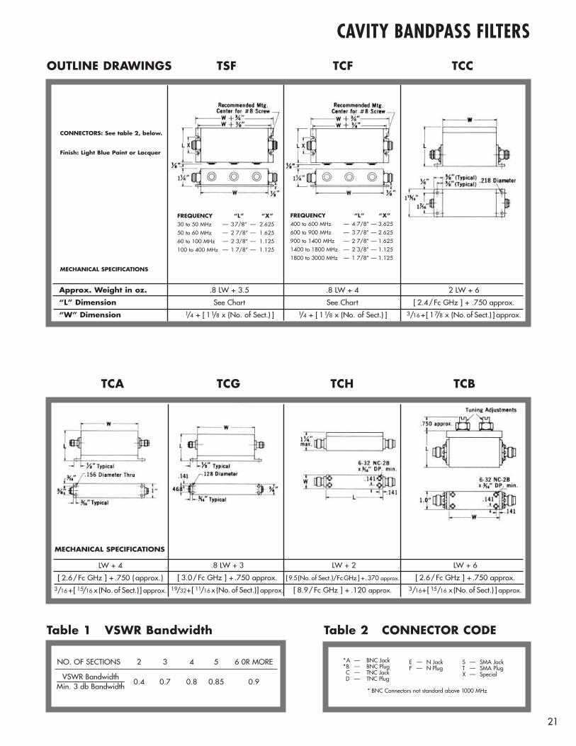
OUTLINE DRAWINGS TSF TCF TCC

Table 1 VSWR Bandwidth Table 2 CONNECTOR CODE

TCA TCG TCH TCB

CONNECTORS: See table 2, below.

Finish: Light Blue Paint or Lacquer



FREQUENCY “L” “X”30 to 50 MHz — 37/8” — 2.625

50 to 60 MHz — 2 7/8” — 1.625

60 to 100 MHz — 2 3/8” — 1.125

100 to 400 MHz — 1 7/8” — 1.125

FREQUENCY “L” “X”400 to 600 MHz — 4 7/8” — 3.625

600 to 900 MHz — 3 7/8” — 2.625

900 to 1400 MHz — 2 7/8” — 1.625

1400 to 1800 MHz — 2 3/8” — 1.125

1800 to 3000 MHz — 1 7/8” — 1.125

Approx. Weight in oz.

“L” Dimension

“W” Dimension

.8 LW + 3.5

See Chart1/4 + [ 11/8 x (No. of Sect.) ]

.8 LW + 4

See Chart1/4 + [ 11/8 x (No. of Sect.) ]

2 LW + 6

[ 2.4/Fc GHz ] + .750 approx.3/16 +[ 17/8 x (No. of Sect.) ] approx.

LW + 4

[ 2.6/Fc GHz ] + .750 (approx.)3/16 +[ 15/16 x (No.of Sect.)] approx.

.8 LW + 3

[ 3.0/Fc GHz ] + .750 approx.19/32+[ 11/16 x (No.of Sect.)] approx.

LW + 6

[ 2.6/Fc GHz ] + .750 approx.3/16+[ 15/16 x (No.of Sect.) ] approx.

LW + 2

[9.5(No.of Sect.)/FcGHz ] +.370 approx.

[ 8.9/Fc GHz ] + .120 approx.

*A — BNC Jack*B — BNC PlugC — TNC JackD — TNC Plug

E — N JackF — N Plug

S — SMA JackT — SMA PlugX — Special


NO. OF SECTIONS 2 3 4 5 6 0R MORE

0.4 0.7 0.8 0.85 0.9VSWR Bandwidth

—————————Min. 3 db Bandwidth

22

DESCRIPTIONTelonic Interdigital Bandpass Filters fill the need for moderateand wide bandwidth filters in the 1.0 to 6.0 GHz spectrum. Thestandard unit is available with as many as 17 sections, to meetextreme selectivity requirements. These 0.1 db Chebyschev filters exhibit almost exact duplicationof the mathematical model. Their skirts or stopbands are geometrically symmetrical.

The specifications for the example shown here as follows:

This unit is a fixed frequency interdigital bandpass filter. It has anominal center frequency of 2,175 MHz and a minimum 3 dbrelative bandwidth of 350 MHz. The maximum insertion loss at2,175 MHz is .55 dB. ( See Insertion Loss Curve page 23). Thenominal input and output impedance is 50 ohms. The maximumVSWR at 2,175 MHz is 1.5:1. The minimum bandwidth overwhich the VSWR remains less than 1.5:1 is 315 MHz (from2,017.5 MHz to 2,332.5 MHz).

The filter has 8 sections and its minimum stopband attenuationis 60 db at 1811.1 MHz and 2595.1 MHz.



Center Frequency Range



Number of Sections

Shock

Vibration

Humidity

Altitude

Temp. Range

Temp. Range

Vibration

Shock

OPE

RA

TIN

G

ST

ORA

GE






Maximum Insertion Loss At Center Frequency

Normal Spec. Limit

Normal Spec. Limit

Normal Spec. Limit

Normal Spec. Limit

Normal Spec. Limit

Normal Spec. Limit

Normal Spec. Limit

Normal Spec. Limit

Normal Spec. Limit

Normal Spec. Limit

Normal Spec. Limit

Normal Spec. Limit

Normal Spec. Limit

Normal Spec. Limit

Normal Spec. Limit

Normal Spec. Limit

*Areas of Interest

*Areas of Interest

*Areas of Interest

Normal Spec. Limit

*Areas of Interest

*Areas of Interest

*Areas of Interest

*Areas of Interest

*Areas of Interest

*Areas of Interest

*Areas of Interest

*Areas of Interest

*Areas of Interest

*Areas of Interest

Normal Spec. Limit

*Areas of Interest

1.0 to 9 GHz ( See Note 1 )

3.0% to 30% ( See Note 1 )

3.0% to 50%

See page 23


Spl. Requirements

100 to1000

5G

15G

2G

10G20G

15G

90%


–54˚C to + 125˚C

– 54˚C to + 100˚C– 62˚C to +150˚C

Up to 100% with Condensation

15G

75G

10 to 100

50 ohms

1.5:1 to 5.0 GHz 2.0:1 to 9 GHz


See Nomograph ( Page 23) Spl. Requirements

4 to 8 ( up to 17 * )

SPECIFICATIONS

Loss Constant ( Fc MHz)300 ( 3 dB BW MHz )

( Fc MHz )

(1500 ) ( 3 dB BW MHz )


INTERDIGITAL BANDPASS FILTERS1,000 TO 9,000 MHz 3.0 TO 30% 3 DB BANDWIDTHS 4 TO 17 SECTIONS

SECTION 5

Finish: Blue Paint


TIF 2175 — 350 — 8 C C

Series

Nominal Center Frequency in MHz


Number of Sections



{

SERIES TIF

OUTLINE DRAWINGS

VSWR Bandwidth


*Submit specific requirements

C — TNC JackD — TNC Plug

†E — Type “N” Jack

†F— Type “N” Plug S — SMA JackT — SMA PlugX — Special

† Type “N” connectors are larger in diameter than the thickness of the filter on which they are mounted.


“L” Dimension

“W” Dimension

.86 LW + 5.52.950.625 + —————— Approx.

( Fc GHz )

2.125 + (.500 ) No. ofSection; Approx.

23

INTERDIGITAL BANDPASS FILTERS ATTENUATION CURVES


BW at X db in MHzMin. 3 db BW MHz

=F4 – F1

F3 – F2

F2 + F3

2

2

2

STOP BAND ATTENUATION:The TIF response curve shown above identifies most of the terms and relationships needed for the calculation of a stop band attenuation specification.

The form factor at any specified attenuation level (X db) is defined as follows:

( I) X db Form Factor =

The form factor nomograph defines the relationship between number of sections, form factor, and attenuation level. Whenever two variables are known, the third can be determined by drawing the indicated straight line.For example:The 60 db form factor for an 8 section filter is 2.24Since these filters are geometrically symmetrical, the following relationship must be used to determine the rejection frequencies. ( II ) F1 F4 = F2 F3, or

( III ) F1 F4 = F2 F3 = FgFg, the geometric center frequency, is not the same as the nominal center frequency which appears in the model number. Fc, the nominal center frequency, is the arithmetic mean of the 3 db band edges.

( IV ) Fc =

In the case of wide bandwidths, the difference between these two numbers is very significant. To calculate the exact rejection frequencies: F3 – F2 = 3 db BW F4 – F1 = X db BW F4 = X db BW + F1From ( II ): F1 ( X db BW + F1 ) = F2 F3 (F1)2 + ( X db BW ) F1 – F2 F3 = 0

( V ) F1 = F2 F3 + (X db BW) – X db BW

( VI ) and F4 = (X db BW) + F12

NOTE 1: Consult factory when selectivity requirement exceeds 8 sections.

= K (N + 0.5)

% BW + 0.1 db

% BW = 100 x 3502175

= 16.1

% BW = 100 x min. 3 db BW MHzNominal Fc MHz

+ 0.1 db = 0.55 db = .85 (8 + 0.5)16.1

INSERTION LOSS:Maximum insertion loss at center frequency

Where: K = Loss constant N = Number of sections

The Insertion Loss Graph defines the loss constant which must be used to calculate the insertion loss specification. For example: MODEL NO. TIF 2175 - 350 - 8CC No. of sections = 8 Center freq. = 2,175 MHz = 2.175 GHz

Loss constant = .85(Read directly from the insertion loss curve at 2.175 GHz.)Therefore:Maximum insertion loss at center freq.

24

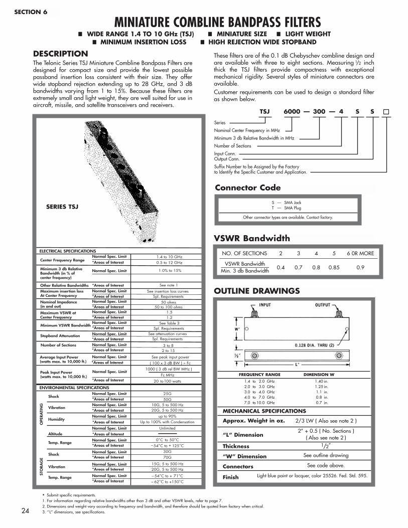
DESCRIPTIONThe Telonic Series TSJ Miniature Combline Bandpass Filters aredesigned for compact size and provide the lowest possiblepassband insertion loss consistent with their size. They offerwide stopband rejection extending up to 28 GHz, and 3 dBbandwidths varying from 1 to 15%. Because these filters areextremely small and light weight, they are well suited for use inaircraft, missile, and satellite transceivers and receivers.

These filters are of the 0.1 dB Chebyschev combline design andare available with three to eight sections. Measuring 1/2 inchthick the TSJ filters provide compactness with exceptionalmechanical rigidity. Several styles of miniature connectors areavailable. Customer requirements can be used to design a standard filteras shown below.



Center Frequency Range

Stopband Attenuation


Number of Sections

Shock

Vibration

Humidity

Altitude

Temp. Range

Temp. Range

Vibration

Shock

OPE

RA

TIN

G

ST

ORA

GE


Peak Input Power (watts max. to 10,000 ft.)





Normal Spec. Limit

Normal Spec. Limit

Normal Spec. Limit

Normal Spec. Limit

Normal Spec. Limit

Normal Spec. Limit

Normal Spec. Limit

Normal Spec. Limit

Normal Spec. Limit

Normal Spec. Limit

Normal Spec. Limit

Normal Spec. Limit

Normal Spec. Limit

*Areas of Interest

*Areas of Interest

*Areas of InterestNormal Spec. Limit *Areas of InterestNormal Spec. Limit *Areas of Interest

*Areas of Interest


*Areas of Interest

*Areas of Interest

*Areas of Interest

*Areas of Interest

Normal Spec. Limit

*Areas of Interest

*Areas of Interest

*Areas of Interest

*Areas of Interest

*Areas of Interest

Normal Spec. Limit *Areas of Interest

0.5 to 12 GHz1.4 to 10 GHz

1.0% to 15%

See insertion loss curves

See note 1

Spl. Requirements

20 to100 watts

25G

30G

10G, 5 to 500 Hz

15G, 5 to 500 Hz20G, 5 to 500 Hz

20G, 5 to 500 Hz

up to 90%

Unlimited

0˚C to 50˚C–54˚C to + 125˚C

– 54˚C to + 71˚C– 62˚C to +150˚C

Up to 100% with Condensation

50G

70G

50 ohms 50 to 100 ohms

1.51.2

See Table 3 Spl. Requirements

See attenuation curvesSpl. Requirements

3 to 82 to 15

( 100 x 3 dB BW ) ÷ Fc

See peak input power

Fc MHz

1000 ( 3 dB rel BW MHz )


MINIATURE COMBLINE BANDPASS FILTERSWIDE RANGE 1.4 TO 10 GHz (TSJ) MINIATURE SIZE LIGHT WEIGHT

MINIMUM INSERTION LOSS HIGH REJECTION WIDE STOPBAND

SECTION 6

TSJ 6000 — 300 — 4 S S

Series



Number of Sections

Input Conn.Output Conn.


SERIES TSJ

OUTLINE DRAWINGS

Connector Code

VSWR Bandwidth

* Submit specific requirements.1. For information regarding relative bandwidths other than 3 dB and other VSWR levels, refer to page 7.2. Dimensions and weight vary according to frequency and bandwidth, and therefore should be quoted from factory when critical. 3. “ L” dimensions, see specifications.

S — SMA JackT — SMA Plug

Other connector types are available. Contact factory.



“L” Dimension

Thickness

“W” Dimension

Connectors

Finish

2/3 LW ( Also see note 2 )

2” + 0.5 ( No. Sections ) ( Also see note 2 )

1/2”

See outline drawing

See code above.

Light blue paint or lacquer, color 25526. Fed. Std. 595.


0.4 0.7 0.8 0.85 0.9VSWR Bandwidth


FREQUENCY RANGE DIMENSION W

1.4 to 2.0 GHz 1.40 in.2.0 to 3.0 GHz 1.25 in.3.0 to 4.0 GHz 1.1 in.4.0 to 7.0 GHz 0.8 in.7.0 to 10.0 GHz 0.7 in.

25

ATTENUATION CURVES

STOP BAND ATTENUATION:This graph shows the minimum stop band attenua-tion in db for Telonic combline bandpass filters. The rejection frequency is plotted in “3 db bandwidthsfrom center frequency.” The exact relationships are:( I ) 3 db bandwidths from Fc

or ( II ) Min. 3 db bandwidth in MHz

Any one of the following parameters may be identified if the other three and the center frequency are known.(1 ) Min. 3 db bandwidth (in MHz).(2 ) Number of sections.(3 ) Rejection Frequency (in MHz).(4 ) Attenuation Level (in dB).

Always verify that the frequency and bandwidth you have selected are within the limitations shownfor that series of filter.

For example ( from Table 1):Given:Center frequency = 6000 MHzMinimum 3 db BW = 300 MHz

Find: Minimum attenuation level at 5190 MHzand 6810 MHz. and No. of sections required.From ( I ) above: 3 db BWs from Fc

Reading directly from the Attenuation curves, points–2.7 and +2.7, we find the minimum attenuation levelof 50 dB. and 54dB respectively.


Min. 3 db BW MHz


3 db BWs from Fc

5190 – 6000 = —————— = –2.7

3006810 – 6000

and —————— = + 2.7300


INSERTION LOSS:

Where: K = Loss constantN = Number of section

For example:TCA 6000 - 300 - 4 - SSNo. of sections = 4Fc = 6000 MHz

K Loss constant = 1.55 ( Read directly from the TSJinsertion curve at 6000 GHz.)Therefore: Max insertion loss at Fc

K ( N + 0.5 ) Max. loss at Fc = —————— + 0.2 db

% BW

100 x min. 3 dB BW MHz % BW = ——————––––––––––––

Nominal Fc MHz

100 x 300 % BW = ————— = 5

6000

1.55 ( 4 + 0.5 ) = —————–––– + 0.21dB = 1.6 db

5

Figure 1. TSJ Attenuation Curves

Figure 2. Insertion Loss Curves

At border or crossover frequencies ( 2, 3, 4, and 7 GHz ) the loss constant ( K ) may be specified for either higher stop band limit or lower insertion loss. For example: ( 1 ) the higher the loss constant,the greater the upper stop band limit but the higher the insertion loss; ( 2 ) the lower the loss constant, the lower the insertion loss but the upper stop band is also slightly decreased ( see Table 5 ).

26

These graphs show the minimum stop band attenuation in dB for the TSCMiniature Filters at different bandwidths. Intermediate values may beinterpolated.For Example: TSC 300 -30 -5SS

To determine the frequencies corresponding to 40 dB attenuation, readfrom stop band attenuation 10% bandwidth the number of 3 dB band-widths away from center frequency corresponding to 40 dB level. Onthe lower frequency side, it is –1.2, and 1.5 on the higher frequency side.The frequency corresponding to 40 dB on the lower skirt = 300 –1.2 x30 = 264 MHz. The frequency corresponding to 40 dB on the upperskirt = 300 +1.5 x 30 = 345 MHz. Based on specific requirements:1. If a certain minimum 3 dB bandwidth and definite rejection at speci-

fied frequencies are required, the appropriate number of sections canbe selected from the attenuation curve. The insertion loss can then bedetermined from the insertion loss curve.

2. If a certain min. 3 dB bandwidth and a definite insertion loss arerequired, the maximum number of sections is found by using theinsertion loss curves, estimating rejection at specified frequencies, ordetermining the frequencies corresponding to any attenuation levelusing the attenuation curves.

In case of special requirements not encompassed in the abovedata, Telonic Berkeley should be contacted directly.

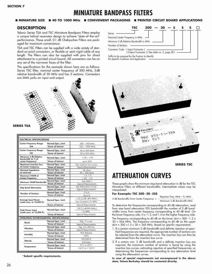
MINIATURE BANDPASS FILTERSMINIATURE SIZE 40 TO 1000 MHz CONVENIENT PACKAGING PRINTED CIRCUIT BOARD APPLICATIONS

SECTION 7

TSC 300 — 30 — 5 S S

Series



Number of Sections

Connector Code – ( Input Connector )( Output Connector ) ( See table no. 2, page 28 )

Suffix to be assigned by the Factory to Identify the Specific Customer and Application.

ATTENUATION CURVES

*Submit specific requirements.

Rejection freq. MHz – Fc MHz3 dB Bandwidths from Center Frequency = ——————————————––––––

Minimum 3 db Bandwidth MHz


OPERATING ENVIRONMENTAL SPECIFICATIONS


Number of Sections

Shock

Vibration

Humidity

Altitude

Temperature


Peak Power Input (watts max. to 10,000 ft.)





Normal Spec. Limit

Normal Spec. Limit

Normal Spec. Limit

Normal Spec. Limit

Normal Spec. Limit

Normal Spec. Limit

Normal Spec. Limit

Normal Spec. Limit

Normal Spec. Limit

Normal Spec. Limit

*Areas of Interest

Center Frequency RangeTSA

Center Frequency RangeTSC

Normal Spec. Limit

*Areas of Interest

*Areas of InterestNormal Spec. Limit *Areas of InterestNormal Spec. Limit *Areas of Interest

*Areas of Interest


*Areas of Interest

*Areas of Interest

*Areas of Interest

*Areas of Interest

Normal Spec. Limit

*Areas of Interest

*Areas of Interest

Normal Spec. Limit

*Areas of Interest

30 to 600 MHz

*Areas of Interest up to 20%

40 to 500 MHz

160 – 1000 MHz200 – 600 MHz

1.0% – 15%

See insertion loss curvesSpecial Requirements

Special Requirements

30g. 11 m sec.

10g, 5 to 500 HzSpecial Requirements

90% Relative

120,000 ft.Unlimited

0˚C to 50˚C–54˚C to + 125˚C

100%


50 ohms 50 – 100 ohms

1.25 : 1.0See Table 1

Special Requirements See Attenuation curvesSpecial Requirements

2 to 6Up to 8

Fc MHz

100 ( 3 dB BW MHz )


Loss Constant x Fc MHz

115 ( 3 dB BW MHz )


1.5: 1.0

SERIES TSC

SERIES TSA

DESCRIPTIONTelonic Series TSA and TSC Miniature Bandpass Filters employa unique helical resonator design to achieve “state-of-the-art”performance. These small, 0.1 dB Chebyschev Filters are pack-aged for maximum convenience.TSA and TSC Filters can be supplied with a wide variety of stan-dard co-axial connectors, or flexible or semi-rigid cable of anylength. The filters can also be supplied with pins for directattachment to a printed circuit board. All connectors can be onany set of the narrower faces of the filter.The specifications for the example shown here are as follows:Series TSC filter, nominal center frequency of 300 MHz, 3dBrelative bandwidth of 30 MHz and has 5 sections. Connectorsare SMA jacks on input and output.

27

ATTENUATION CURVES

28


INSERTION LOSS:

The approximate value for insertion loss at center frequency is found with the following formula.

Where: K = Loss constantN = Number of sections *

The loss constant is read directly from the insertion loss graph at the point which corresponds to the center frequency of the filter.

For example:

A 5 section filter at 300 MHz with a bandwidth of 30 MHz would have an approximate insertion loss of 1.5 db:

KN Insertion loss in db = ———— + 0.2

% BW

100 x min. 3 dB BW MHz % BW = ——————––––––––––––

Fc MHz

2.6 x 5 Ins. Loss = ———— + 0.2 = 1.5 db

10

Table 1 VSWR Bandwidth Table 2 CONNECTOR CODE

StandardP — Pins for printed circuit boardS — SMA JackT — SMA PlugAvailableX — All other configurations including semi rigid, RG188,

RG196 ( Specify requirement ).


0.4 0.7 0.8 0.85 0.9VSWR Bandwidth


OUTLINE DRAWINGS


Size

Weight

3/8 x 11/16 x L1, L1 = 11/2 + n––4

approx. where n = no. of sections

Usually less than 1.5 oz. max without connector.


Size

Weight

1/2 x 11/2 x L1, L1 = N ( 1”) + 0.5” where N = no. of sections

Approx. 25 grams /Linear inch

* Consult factory for insertion loss when N = 2

The products covered in this catalog represent Telonic Berkeley’s generalfilter product line. We specialize in fulfilling your unique filter requirements andwelcome the opportunity to discuss your specifications with you.

We have the capabilities to build filters to meet your exact needs. For moreinformation, please call our Customer Service Department:

Web: www.telonicberkeley.comemail: [email protected]

(800) 854-2436

FAX: (949) 497-7331

Our Toll Free Telephone:

© March 2003, Telonic Berkeley, Inc. Printed in U.S.A. 1M1195

(800) 854-2436

Telonic Berkeley, Inc.P.O. Box 277

Laguna Beach, CA 92652(949) 494-9401

FAX: (949) 497-7331Web: www.telonicberkeley.comemail: [email protected]

Telonic Berkeley, Inc. manufacturing facility in Laguna Beach, California.

Our Toll Free Telephone:

telonic fixed frequency filters - test equipment · pdf fileseries tsa — smallest...

Documents