tecnai on-line help manual -- modes
TRANSCRIPT

Tecnai on -line help Modes 1 Modes_12to30_A4.doc Software version 2
Tecnai on-line help manual -- Modes Table of Contents 1 Standard operating procedures..............................................................................................................3
1.1 Aperture centering ..........................................................................................................................3 1.1.1 Condenser aperture.................................................................................................................3 1.1.2 Contrast aperture.....................................................................................................................3 1.1.3 Diffraction aperture ..................................................................................................................4
1.2 Setting the eucentric height............................................................................................................5 1.3 Focusing..........................................................................................................................................6
1.3.1 Wobbler....................................................................................................................................6 1.3.2 Focused beam.........................................................................................................................8 1.3.3 Contrast-enhancement............................................................................................................8 1.3.4 Diffraction focus.......................................................................................................................8 1.3.5 Small screen and binoculars ...................................................................................................9
1.4 Correction of astigmatism...............................................................................................................9 1.4.1 Condenser stigmation............................................................................................................10 1.4.2 Image stigmation ...................................................................................................................10 1.4.3 Diffraction stigmation .............................................................................................................17
2 Calibration procedures .........................................................................................................................18 2.1 Magnification calibration ...............................................................................................................18 2.2 Camera-length calibration.............................................................................................................18 2.3 Image-diffraction rotation angle ....................................................................................................19
3 Bright-field imaging...............................................................................................................................20 3.1 Standard method..........................................................................................................................20 3.2 Working with magnetic specimens...............................................................................................20
3.2.1 Counteracting the magnetism of the specimen.....................................................................20 3.2.2 Lorenz microscopy.................................................................................................................21
4 Dark-field imaging.................................................................................................................................21 4.1 Axial dark-field imaging.................................................................................................................21 4.2 Off-axis imaging ............................................................................................................................22
5 Diffraction..............................................................................................................................................23 5.1 Focusing in diffraction...................................................................................................................23 5.2 The shadow image........................................................................................................................24 5.3 Selected-area diffraction...............................................................................................................25 5.4 Diffraction without selected-area aperture....................................................................................26 5.5 Standard convergent-beam diffraction .........................................................................................27
5.5.1 Orienting the crystal...............................................................................................................27 5.5.2 Fine-tuning pattern .................................................................................................................27
5.6 Large-angle convergent beam (LACBED/Tanaka) ......................................................................27 6 Analysis ................................................................................................................................................29
6.1 EDX analysis.................................................................................................................................29 6.1.1 Microprobe versus nanoprobe...............................................................................................29 6.1.2 Shadowing angle...................................................................................................................29
6.2 EELS analysis...............................................................................................................................30 6.2.1 Determining spectrometer acceptance angle β ....................................................................30
7 STEM....................................................................................................................................................32 7.1 STEM principles............................................................................................................................32 7.2 The importance of the pivot points...............................................................................................33 7.3 Detectors.......................................................................................................................................34
Tecnai on -line help Modes 2 Modes_12to30_A4.doc Software version 2
7.3.1 Bright-Field (BF) detector......................................................................................................34 7.3.2 Dark-Field (DF) detector........................................................................................................34 7.3.3 High-Angle Annular Dark-Field (HAADF) detector...............................................................34 7.3.4 Secondary-Electron (SE) detector.........................................................................................35 7.3.5 BackScattered-electron (BS) detector...................................................................................35 7.3.6 Energy-Dispersive X-ray (EDX) detector ..............................................................................35 7.3.7 Electron Energy-Loss Spectrometer (EELS) ........................................................................35
7.4 Detector alignment........................................................................................................................36 7.5 STEM adjustments - an in-depth explanation..............................................................................36 7.6 STEM Operation ...........................................................................................................................36
7.6.1 Tecnai Imaging & Analysis ....................................................................................................36 7.6.2 Resolution and frame size .....................................................................................................37 7.6.3 Detectors and channels.........................................................................................................38 7.6.4 Detector control .....................................................................................................................38 7.6.5 Procedure for manual setting of detector contrast and brightness.......................................39 7.6.6 Filters .....................................................................................................................................40
8 EFTEM..................................................................................................................................................42 8.1 General introduction to energy filtering ........................................................................................42 8.2 The (post-column) Imaging Filter..................................................................................................42 8.3 EFTEM on the Tecnai microscope...............................................................................................43 8.4 Important concepts in Tecnai EFTEM..........................................................................................43
8.4.1 Image, diffraction pattern and spectrum................................................................................43 8.4.2 Cross-over correction ............................................................................................................44 8.4.3 Normalizations.......................................................................................................................44 8.4.4 SA diffraction..........................................................................................................................45

Tecnai on -line help Modes 3 Modes_12to30_A4.doc Software version 2
1 Standard operating procedures
1.1 Aperture centering
1.1.1 Condenser aperture The condenser aperture is the illuminating -beam limiting aperture in the column. The alignment of the aperture is important for two aspects: 1. For convenience, to make the expanding (defocused) and contracting (focused) beam stay centered
on the screen (thereby making it unnecessary to adjust the beam position continuously). 2. To ensure reproducible illuminating conditions. Misalignment of the condenser aperture leads to a
beam tilt (and thus a change in the rotation center). In principle, it is possible to adjust the rotation center whenever the aperture is changed. In practice, it is much easier to make sure the aperture centering is reproducible - and thus the rotation center stays the same.
Note 1: Because of the latter aspect, it is much more important to align the aperture in a reproducible manner (always following the same procedure; that is, use the same magnification and defocus the beam by the same amount each time) than having a ‘perfectly’ aligned aperture (by whatever criterion). Procedure • Select a suitable magnification (the choice is up to user, but select the same one each time). • Focus the illumination using the Intensity knob and center the beam, as necessary, using the beam
shift (left-hand track ball). • Defocus the illumination clockwise (overfocus) by a set amount (e.g. to the 4 centimeter circle on the
viewing screen). The illuminated area should still be around the center of the screen. If not, align the condenser aperture using the mechanical aperture controls to achieve this condition.
• Repeat the last two steps until the illuminated area remains centered. Note 2: There typically is a difference between the aligned condenser aperture in the microprobe and nanoprobe modes (requiring adjustment when switching be tween these modes). This mechanical misalignment is a consequence of the difficulty of mechanical alignment of the minicondenser lens. Generally, the misalignment is readily apparent when changing from one mode to another. However, when switching to STEM (in essence a nanoprobe mode) from microprobe, this misalignment may not be apparent. It is advised, therefore, to proceed via nanoprobe (for centring the aperture) when going to STEM.
1.1.2 Contrast aperture The contrast aperture eliminates diffracted beams (and, depending on the aperture size, energy-loss electrons) from the beam, thereby giving contrast in the image. In the high-magnification range, the objective aperture (generally located at the level of the diffraction pattern) is the contrast-forming aperture. In the low-magnification range, the objective lens is (nearly) off and the diffraction pattern is located at the selected -area aperture. The latter thus is the contrast-forming aperture for the low-magnification range (it is, however, rarely used in the low-magnification range). High-magnification range – objective aperture When the objective aperture is used, a number of diffracted electrons is scattered back and may interacts with the specimen. These backscattered electrons counteract the losses of secondary electrons and thereby reduce or eliminate charging of the specimen. The latter can have disastrous effects on poorly conducting specimens like biological ones, where the charging is seen as a ‘blowing’ up (in appearance like a balloon) of the specimen, after which the specimen often blows apart. Keeping the
Tecnai on -line help Modes 4 Modes_12to30_A4.doc Software version 2
objective aperture in is one way of preventing the destruction of biological specimens. Another method is to keep part of the illumination on a grid bar. The latter method is dangerous, however, because the specimen with blow up as soon as the beam is no longer on the grid bar (e.g. when the specimen or beam is moved). Neither method can be used for EDX analysis (which requires that the objective aperture is removed; and flooding the EDX detector with X rays from the grid bar also will not be conducive to good analysis) and there a properly conducting specimen is required (carbon coating or put on a conducting carbon film). In less strongly insulating specimen, charging may appear as a shivering or repeated jumping of the specimen. It may be possible to reduce the charging by selecting a smaller beam (lower total current) and/or smaller objective aperture. Once again, a carbon coating may prevent charging altogether. Procedure 1 • Select a suitable magnification (as required by the type of image, e.g. 5kx to 20kx for intermediate -
magnification work or 100kx for high -resolution work). • Set proper illuminating conditions (beam defocused – overfocus, i.e. clockwise with intensity – to
illuminate the whole viewing screen or just beyond the rim of the screen). • Switch to diffraction. • Select a camera length of approximately 500 mm. • Insert the required objective aperture into the beam and center it around the central beam spot using
the mechanical aperture controls. Procedure 2 • Insert the objective aperture. • If no bright-field image is visible at all, it may be necessary to use procedure 1 for rough centering
first. Otherwise, shift the aperture until there is no cut-off of the illuminated area visible (if n ecessary defocus/focus the beam).
Low-magnification range – selected-area aperture Procedure • Select a suitable magnification (around 500x). • Set proper illuminating conditions (beam defocused – overfocus, i.e. clockwise with intensity – to
illuminate the whole viewing screen or just beyond the rim of the screen). • Switch to diffraction (LAD). • Select a low camera length (typically the fourth of the LAD range). • Insert the largest selected -area aperture into the beam and center it around the central beam spot
using the mechanical aperture controls.
1.1.3 Diffraction aperture Diffraction can be done with area selection by means of an aperture (selected-area diffraction) or simply by illuminating an area with the beam (typically convergent beam diffraction with a focused beam though it is not strictly necessary to focus the beam completely). High-magnification range – selected-area aperture In the high-magnification range, the selected -area (SA) aperture acts as the area-selection tool for diffraction work. In the SA magnification range, the first intermediate image coincides with the level of the SA aperture. This range is therefore the optimum for high -quality selected-area diffraction work. The Mi (between LM and SA) and Mh ranges have their first intermediate images below and above the SA aperture level, respectively, and are therefore not as well suited as starting point for SA diffraction (but SA diffraction is very well possible from these ranges).

Tecnai on -line help Modes 5 Modes_12to30_A4.doc Software version 2
Note 1: The Tecnai microscope uses (small) image shifts between different magnification steps to align the different magnifications (the image stays centered when the magnification is changed). Because this alignment is executed with the image shift deflection coils, located between the objective lens and the SA aperture, it is impossible to shift both the image and shadow of the SA aperture at the same time (the shift takes place between them). The consequence of the image alignment is therefore an apparent shift of the SA aperture when the magnification is changed. Always select the appropriate magnification first and then insert and center the SA aperture. Note 2: If the diffraction shift pivot point is not aligned properly, changing the diffraction shift (either intentionally by the user or simply because the camera length is changed and the new camera length has a different alignment) will lead to an image shift as well. Since this image shift takes place above the SA aperture, the specimen area will move out of the aperture and the diffraction pattern will come form a different area than the one intended. It is therefore important to ensure that the pivot points of the image coils (the image and - especially – the diffraction shift pivot points) are aligned properly. Because the diffraction shift pivot point is very sensitive to the objective-lens current, it is also important to make sure that the specimen is at the eucentric height (additionally the eucentric height is important for accurate values of camera length and magnification). Procedure • Obtain an image at a suitable magnification. • Insert the SA aperture and center it on the area of interest (by preference near the screen center)
using the mechanical aperture controls. • If no aperture is visible upon insertion, reduce the magnification or select and center a larger aperture
first before continuing on to the aperture with the required size. Note: If the objective aperture is smaller than the central beam, use either a smaller C2 aperture, defocus the beam with Intensity, or use a larger objective aperture. Low-magnification range – objective aperture Procedure • Obtain an image at a suitable magnification. • Insert the objective aperture and center it on the area of interest (by preference near the screen
center) using the mechanical aperture controls. • If no aperture is visible upon insertion, reduce the magnification or select and center a larger aperture
first before continuing on to the aperture with the required size.
1.2 Setting the eucentric height The eucentric height is important in the microscope. It is not only convenient that the area of interest stays centered when tilting around the α tilt axis (but if you never tilt anyway, this feature may be of little interest), but it also defines a reference value for the objective -lens current. The normal changes made to the objective for focusing have little effect, but stronger changes (changes in focus by several tens of micrometers or more) can have considerable effect on: • The effective magnifications and camera lengths (the objective lens not only focuses the image but
also contributes the largest magnification of any lens in the system; strong changes in objective lens current change this magnification and thereby also the final magnification and camera length).
• Proper alignments.

Tecnai on -line help Modes 6 Modes_12to30_A4.doc Software version 2
There are several methods for setting the eucentric height. Procedure 1 : the α wobbler • Activate the a wobbler of the CompuStage, typically using the maximum tilt angle available (15° on
all instruments except U-TWIN instruments where the maximum is 5°). For magnetic specimen is may be advisable to use a smaller angle (because of the effect of the specimen’s magnetism on the objective -lens field).
• Minimize the sideways motion of the image with the Z axis height control. • Switch the α wobbler off. Procedure 2 : the focus wobbler • Press the Eucentric focus button to set the objective lens to the eucentric height preset (this method
presumes the microscope has been aligned properly and this preset has been set). • Press the Wobbler button and minimize the distance between the two apparent images with Z axis
height control. • When done, switch the wobbler off. Procedure 3 : minimize the α tilt displacement • Reset the α tilt to 0° (the Stage Control in the Stage Control Panel flap-out has a function for this). • Find and center an easily recognizable feature in the specimen. • Tilt the stage with the α tilt by a small amount (~5°). • If the feature moved away from center, move it back with the Z axis height control. • Reset the α tilt to 0° again and repeat until the feature doesn’t move when the α tilt is used.
1.3 Focusing There are many ways of focusing the image. Some of the more common ones are described below. One simple tool always available is the Eucentric focus function which works both in image and diffraction. In image the Eucentric focus sets the focus to the value for the eucentric height. Assuming that the specimen is at the eucentric height, this eucentric focus function provides a quick method for getting close to the proper focus. The actual value set is set in the various alignment procedures (HM Image, LM Image, Nanoprobe Image). In diffraction, the Eucentric focus function resets the user-defined focus to zero. When properly aligned (by means of the Camera Length Focus in the HM Image procedure), this effectively means that the focus is set to the back-focal plane (see section 1.3.4).
1.3.1 Wobbler The function of the wobbler is to deflect the beam alternately to either side of the optical axis. When the objective lens is focused exactly on the specimen plane, no change in the image is apparent. However, when the objective lens is focused above or below the specimen plane there is an apparent double image so the wobbler is very useful for emphasizing focusing errors. The direction of the wobbler effect should be selected perpendicular to the direction of the structures to be focused. This is adjusted using the Multifunction-X knob. The amplitude of the wobbler effect is adjusted using the Multifunction-Y knob. This angle should be adapted to the size of the objective lens aperture otherwise loss of intensity will occur when the wobbler is operated (if the beam tilt become too high the transmitted beam is stopped by the objective aperture).
Tecnai on -line help Modes 7 Modes_12to30_A4.doc Software version 2
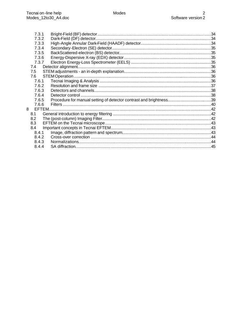
The procedure is as follows: • Insert a specimen, adjust its height and focus the image. • Press Diffraction pushbutton (LED on). • Select a camera length of approximately 600 mm. • Focus the illumination using the Intensity knob. • Ensure that the objective aperture is correctly centered. • Press the Wobbler pushbutton: two spots should appear within the area of the objective aperture. If
not, lower the wobbler amplitude until they do. • Press Diffraction pushbutton (LED off) and focus the image to minimum blur. • When finished, press the Wobbler button once again to switch it off.
Focus without use of the wobbler. Focus after use of the wobbler.
Out of focus - wobbler in chosen direction. Out of focus - wobbler perpendicular to c.
Tecnai on -line help Modes 8 Modes_12to30_A4.doc Software version 2
1.3.2 Focused beam When the beam is focused on the specimen (or slightly defocused), the beam should look exactly the same as when it passes through a hole in the specimen. If the beam has a diffuse halo around it, the specimen is not in focus. Focus to minimize the halo (it will merge with the beam when the specimen is in focus). In crystalline specimens a diffraction pattern may also appear superimposed on the image. Once again, focus is attained when the diffraction is minimized. This method is especially useful in the nanoprobe mode or without an objective aperture in. Note: The appearance of multiple images (one from the transmitted beam and other ones from strong diffracted beams) is a consequence of the spherical aberration of the objective lens (and the absence of an aperture to block the diffracted beams). Even at true focus, these multiple images may remain visible. In general this aspect is not troublesome, except in the low-magnification range. When the objective lens is (nearly) off, the diffraction lens is used as the ‘objective’ lens. When used in this way, the diffraction lens has a very long focal length (hence the very strong contrast in the LM image) and also high spherical aberration. Because of the latter, the multiple images may be pronounced, making it very difficult to focus (the images will not merge together, even at focus).
1.3.3 Contrast-enhancement In some cases (especially in biology) it is advisable to set the focus deliberately a certain amount underfocus to enhance contrast. The amount of underfocus set depends on the magnification (at high magnification an underfocus image looks blurry while the same amount of underfocus at lower magnifications may look sharp) and the degree of contrast enhancement required.
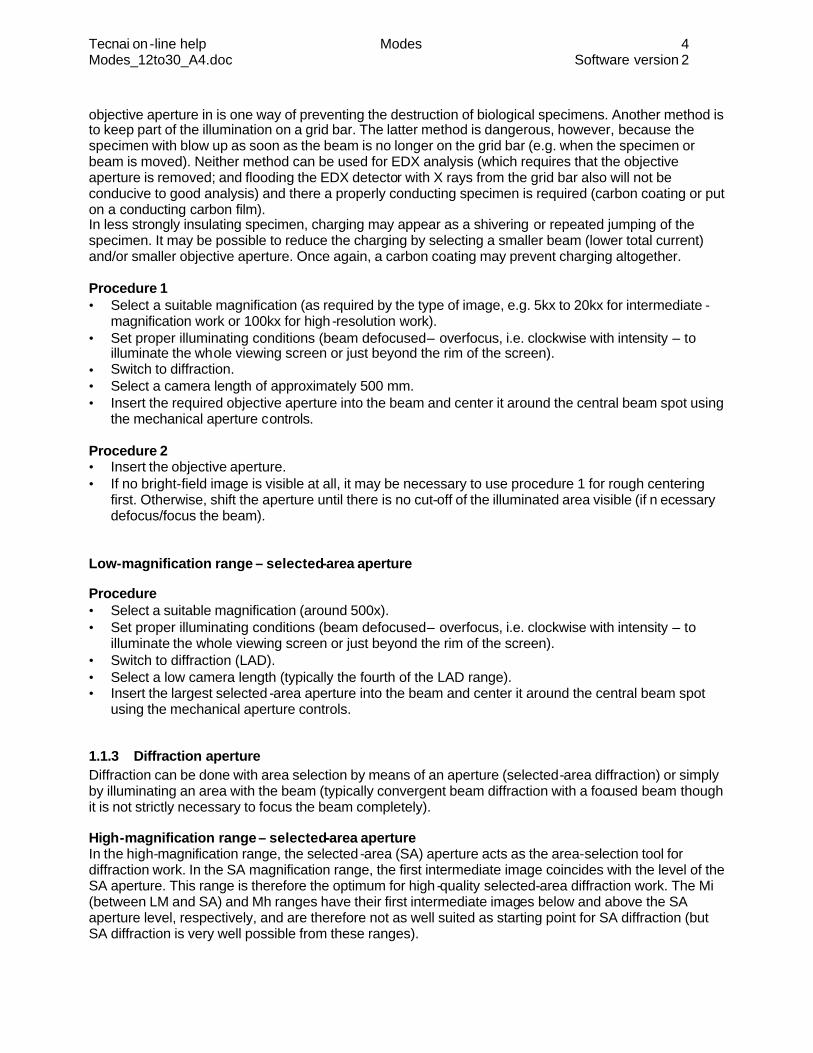
1.3.4 Diffraction focus Unlike the image, the diffraction pattern does not have a clear criterion for establishing when it is in focus. Often it is presumed to be 'in focus' when the pattern has spots that are as small as possible. This is not strictly true. The diffraction pattern is in focus when the focus lies at the back-focal plane of the objective lens. Only when the incident beam is parallel does the cross-over lie in the back-focal plane.
With a parallel beam incident on the specimen (grey), the objective lens focuses the electrons into a cross-over whose position coincides with the back-focal plane (and thus the true diffraction focus).
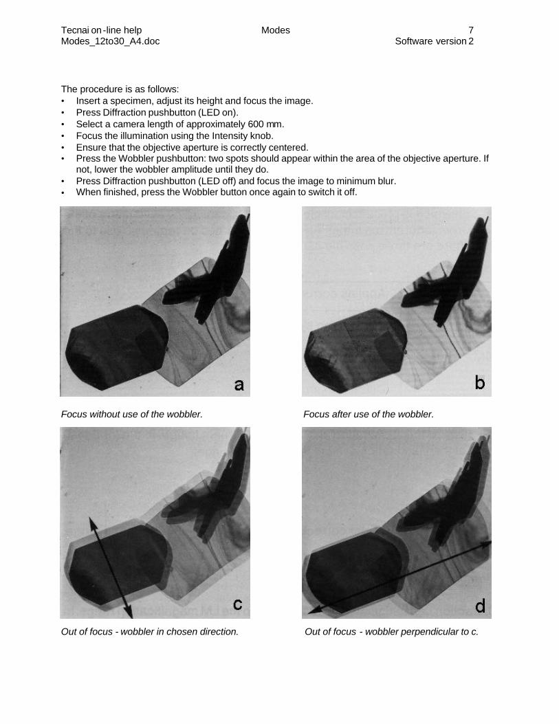
When the beam is convergent (but not wholly focused), there still is a cross-over but it is displaced from the back-focal plane upwards (in the extreme case, a fully focused beam, the cross-over lies at the image plane).
Tecnai on -line help Modes 9 Modes_12to30_A4.doc Software version 2
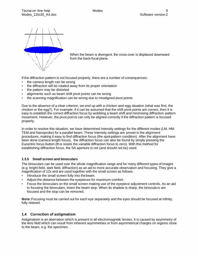
When the beam is divergent, the cross-over is displaced downward from the back-focal plane.
If the diffraction pattern is not focused properly, there are a number of consequences: • the camera length can be wrong • the diffraction will be rotated away from its proper orientation • the pattern may be distorted • alignments such as beam shift pivot points can be wrong • the scanning magnification can be wrong due to misaligned pivot points Due to the absence of a clear criterion, we end up with a chicken -and-egg situation (what was first, the chicken or the egg?). For example, if it can be assumed that the shift pivot points are correct, then it is easy to establish the correct diffraction focus by wobbling a beam shift and minimising diffraction -pattern movement. However, the pivot poin ts can only be aligned correctly if the diffraction pattern is focused properly. In order to resolve this situation, we have determined Intensity settings for the different modes (LM, HM-TEM and Nanoprobe) for a parallel beam. These Intensity settings are preset in the alignment procedures, making it easy to find diffraction focus (the spot-pattern condition). After the alignment have been done (camera length focus), the diffraction focus can also be found by simply pressing the Eucentric focus button (th is resets the variable diffraction focus to zero). With this method for establishing diffraction focus, the SA aperture is not (and should not be) used.
1.3.5 Small screen and binoculars The binoculars can be used over the whole magnification range and for many different types of images (e.g. bright field, dark field, diffraction) as an aid to more accurate observation and focusing. They give a magnification of 12x and are used together with the small screen as follows: • Introduce the small screen fully into the beam. • Adjust the distance between the eyepieces for maximum comfort. • Focus the binoculars on the small screen making use of the eyepiece adjustment controls. As an aid
to focusing the binoculars, insert the beam stop. When its shadow is sharp, the binocula rs are focused and the stop can be removed.
Note: Focusing must be carried out for each eye separately and the eyes should be focused at infinity, fully relaxed.
1.4 Correction of astigmatism Astigmatism is an aberration which is present in all electromagnetic lenses. It is caused by asymmetry of the lens field which can result from inherent asymmetries or from asymmetrical charges on regions close to the beam, e.g. the specimen.
Tecnai on -line help Modes 10 Modes_12to30_A4.doc Software version 2
1.4.1 Condenser stigmation • Make sure that the image is focused and reasonably well stigmated (it is not very critical, but if the
image stigmation is much off, the beam may appear astigmatic due to the image astigmatism). • Remove the specimen and the objective aperture from the beam. • In the microprobe mode (LM, HM) select a workset tab containing the Stigmator Control panel and
press the Condenser stigmator button (green LED on). In Nanoprobe or STEM, the same can be done, but it is also sufficient to press the Stigmator button on the left-hand Control Pad (the condenser stigmator is the default stigmator in these modes).
• Astigmatism is corrected when the focused beam remains as circular as possible when going through beam focus (Intensity). Adjust this using the Multifunction -X and Y control knobs. Alternatively, the filament can be undersaturated until structure is visible in the focused beam. Astigmatism is corrected when this structure is as sharp as possible (adjust Intensity, Multifunction -X and Y).
1.4.2 Image stigmation Three factors can cause image astigmatism: 1. Asymmetry of the objective lens. 2. Dirt on or charging of the objective aperture. 3. The specimen itself. The influence of the specimen on the observed astigmatism can be
considerable, particularly in cases where an insulating specimen collects charge, either as a whole or locally. Magnetic specimens also cause strong astigmatism.
High-magnification range Astigmatism is most easily observed on the screen when viewing Fresnel fringes. These fringes result from diffraction phenomena that occur at sharp edges of a specimen when the objective lens is slightly underfocused or overfocused. When the image is underfocused (objective lens weaker than focus), the Fresnel fringe appears as a bright line round the edge of the detail selected. If the detail is a hole, the line will appear on the inside. When the image is overfocused (objective lens stronger than focus), the Fresnel fringe appears as a dark line but otherwise has the same characteristics as in the underfocused condition. With a perfectly symmetrical objective lens field, the fringes will be of uniform width. With an asymmetrical (astigmatic) objective lens, the fringes will also be asymmetrical and, close to the focus, part of the hole will have a bright fringe and the other part a dark fringe associated with it. For more information about astigmatism in electron lenses, reference is made to the many text books on electron optics, for example: Transmission Electron Microscopy (2ed.), L. Reimer (1989), Springer-Verlag, Berlin. Experimental High Resolution Electron Microscopy (2ed.), J. C. H. Spence, Oxford University Press, New York, Oxford. A typical test specimen for measurement and correction of astigmatism is a very thin carbon support film with small perforations. This film must be of a conducting material, because of the high magnifications and thus high beam intensities that will be used and great care should be taken to ensure that the film adheres firmly to the supporting grid. Very small spherical particles can also be used, but this is not advisable because of the possibility that the projected periphery of the particles may not originate from a single plane. In that case, there will be an inherent change of focus around the particle which cannot be distinguished from astigmatism and will thus be corrected when correcting the astigmatism.

Tecnai on -line help Modes 11 Modes_12to30_A4.doc Software version 2
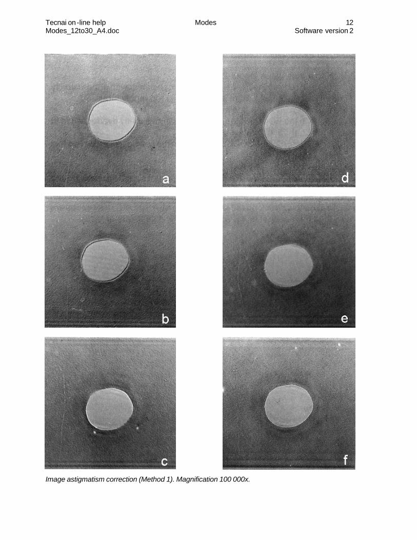
In general, accurate correction of astigmatism can be made only at high magnification and under good image visibility conditions. This implies high beam intensity on the specimen. In order to compensate for objective lens astigmatism applicable to the M and SA magnification range, an electromagnetic astigmatism corrector is built into the microscope below the objective lens. There are two possible methods for correcting the astigmatism. In the first, use is made of the special test specimen described above. In the second, use is made of the fact that, at high magnification, all thin objects have a substructure in the size range 0.3-0.2 nm and use is then made of the point/focal line phenomena. The latter method is preferred because of the influence of the specimen itself, causing astigmatism to vary for different areas of the specimen. The method requires some experience, however, and it is recommended that this experience be gained, where necessary, by comparing the effect of the two methods on the special test specimen. Method 1 This method is illustrated in the figure which shows two focal series with astigmatism uncorrected (left-hand side, figure a to c) and corrected (right-hand side, figure d to f). The procedure is as follows: • Obtain a TEM BF image of the test specimen at high magnification (around 100 000x). • Press the Stigmator pushbutton (LED illuminated). • Select a very small hole. This should be of such a size that it is visible in its entirety through the
binoculars at the highest magnification used. • Adjust the Focus until the entire hole is overfocused yet close enough to focus for the fringe
asymmetry to be visible (black fringe inside the hole, Fig. a). Change of focus (lower excitation of the objective lens) produces the images in Figs. b and c.
• Adjust the Multifunction knobs so that the Fresnel fringe is symmetrical when the objective lens is very slightly overfocused.
• To perform this procedure, start adjustment by turning one of the Multifunction knobs until the setting for minimum astigmatism is obtained (best symmetry for overfocused image). Then adjust the other knob for minimum astigmatism.
• Repeat the preceding step at a higher magnification and with smaller focusing step sizes until adequate correction is obtained (Fig. d). The criterion for this is that no asymmetry of the fringe can be seen at one or two step positions overfocus of the finest step size. Change of focus (lower excitation of the objective lens) gives rise to the images in Figs. e and f.
Tecnai on -line help Modes 12 Modes_12to30_A4.doc Software version 2
Image astigmatism correction (Method 1). Magnification 100 000x.

Tecnai on -line help Modes 13 Modes_12to30_A4.doc Software version 2
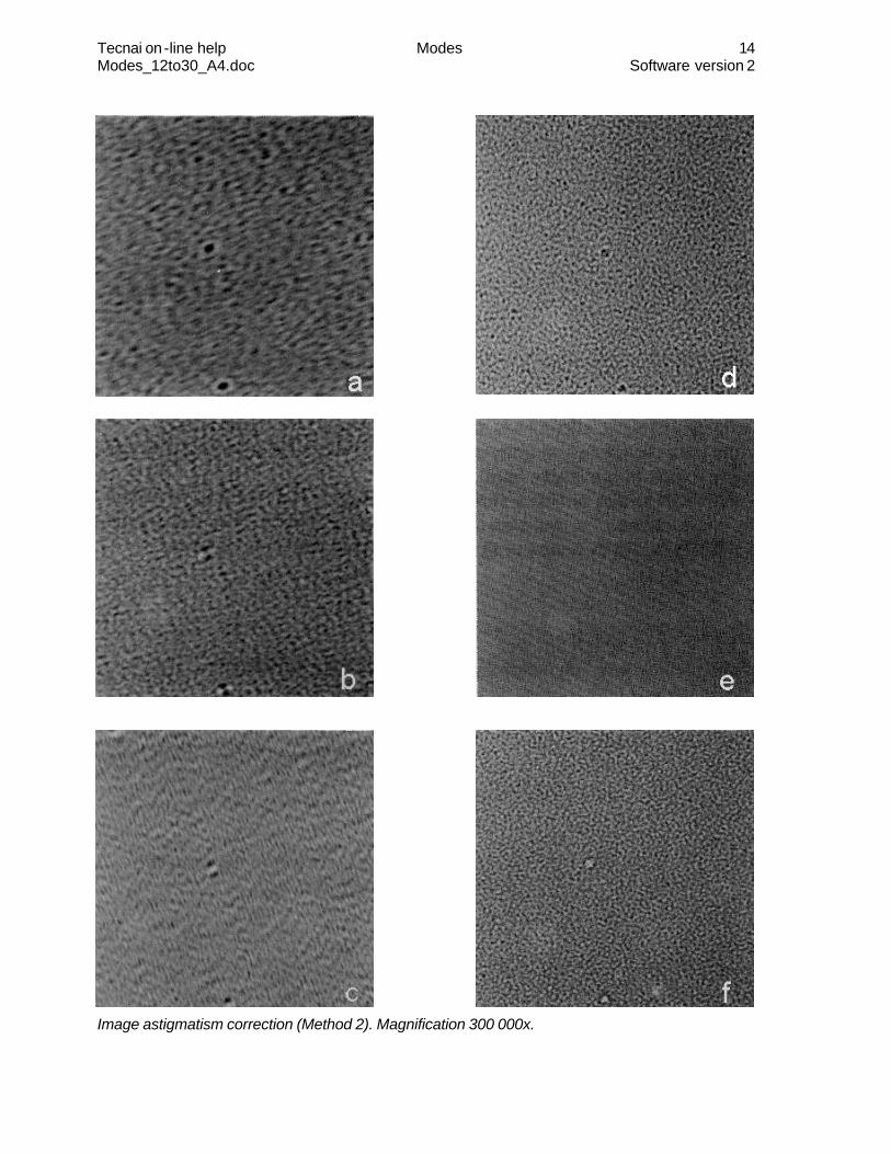
Method 2 This method is shown in the figure below which shows two focal series with astigmatism uncorrected (left-hand side, figure a to c) and corrected (right-hand side, figure d to f). The procedure for correction of the astigmatism on the specimen sub -structure is as follows: • Select and center a small C2 aperture (50 um). • Set the magnification to a high value (about 200 000x). • Set the spot size to step 3 and reduce the Intensity as far as possible to be consistent with good
visibility of the structure (the contrast of the substructure disappears if the beam is focused too much).
• Select a thin part of the specimen showing fine structure. • Select focus step 2 and with the focus knob, vary the objective lens from slightly overfocused to
slightly underfocused (total change in focal length less than 1 um). • Look for the line foci (Figs. a, b and c). Set the Focus knob halfway between the settings for these
two foci (Fig. b). • Press the Stigmator pushbutton (LED illuminated). • Adjust the two Multifunction knobs one at a time to decrease the apparent size of the background
structure and at the same time reduce the line effect (Fig. d, e and f) on changing to over and underfocus.
• Repeat the preceding step (at a higher magnification if desired) until the focal distance between the line foci is as small as required (3 nm or even smaller is possible).
Note: With very thin specimens the substructure disappears from the visual image at focus. This can be used as a very sensitive check on the final correction. The two Multifunction knobs are then used to reduce the contrast of the substructure until it finally disappears at focus.
Tecnai on -line help Modes 14 Modes_12to30_A4.doc Software version 2
Image astigmatism correction (Method 2). Magnification 300 000x.

Tecnai on -line help Modes 15 Modes_12to30_A4.doc Software version 2
LM magnification range When operating in the LM mode, it is possible that some astigmatism will be observed at the higher magnifications. If it is required to make photographs in this mode, astigmatism in the image can be corrected by one of the following methods. Note: The (default) stigmator used in LM is the diffraction stigmator. Method 1 This method is the same as method 1 for the high -magnification range. • Insert a test specimen (as described before under method 1 for the high-magnification range). • Press the Stigmator pushbutton (LED illuminated). • Insert and center the second-largest SA aperture. • Select the highest LM magnification. At this stage, Fresnel diffraction fringes should be observed
around the inside of the holes in the specimen. • If these fringes are not symmetrical, correct the astigmatism using the Multifunction knobs. • Adjust the Focus until the entire hole is slightly overfocused, yet close enough to focus for the fringe
asymmetry to be visible (black fringe inside hole). • Adjust the Multifunction knobs one at a time so that the Fresnel fringe is symmetrical when the image
is very slightly overfocused. This is achieved by turning the two Multifunction knobs until a setting for minimum astigmatism is obtained.
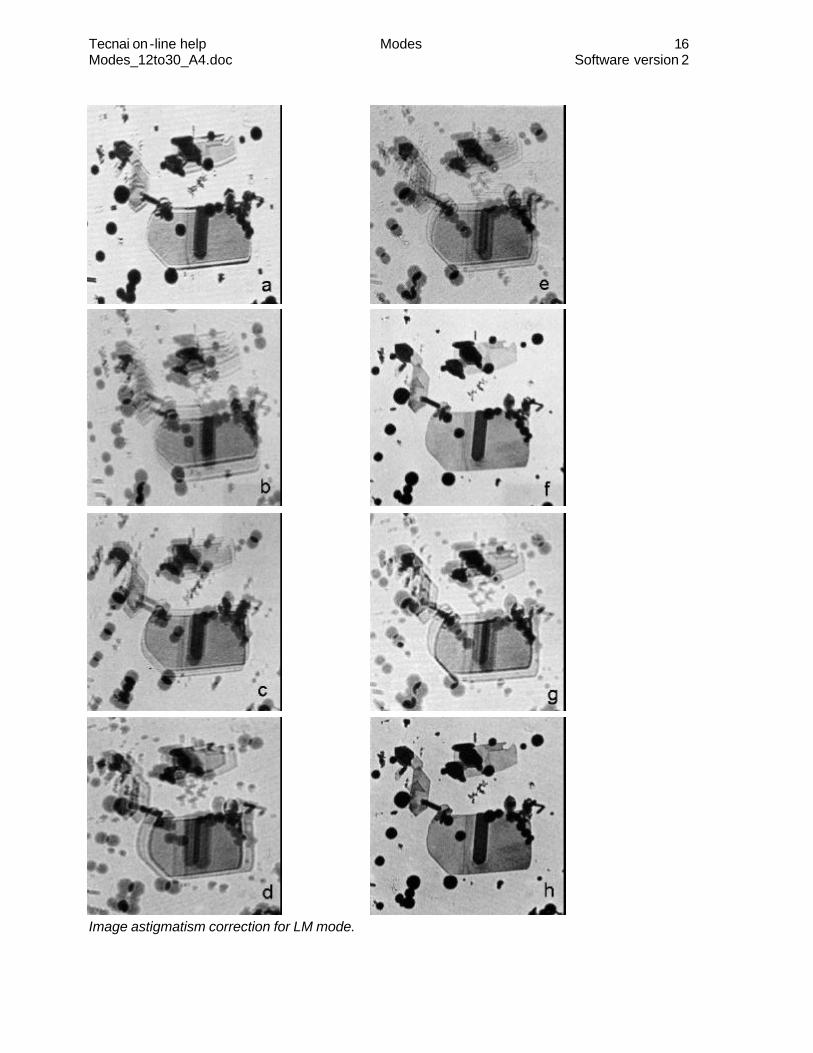
Method 2 This method is illustrated in the figure below showing: a : An overfocused image with asymmetrical Fresnel fringes indicating astigmatism b, c, d : A through-focus series with wobbler in use with astigmatism uncorrected. e, f, g : A through-focus series with wobbler in use with astigmatism corrected. h : A corrected, focused image, wobbler not in use. • Ensure that a platinum aperture not smaller than 150 mm is mounted in the selected-area aperture
holder and that it is clean. • Insert a specimen and center a suitable detail. • Center the selected-area aperture. • Press the Stigmator pushbutton (LED illuminated). • Set the magnification to the highest LM value. • Press the Wobbler pushbutton. • Focus the image so that the blurred image details (Fig. c) are as nearly coincident as possible. • Adjust the Multifunction knobs until the image details are coincident (Fig. f). • Repeat the last two steps.
Tecnai on -line help Modes 16 Modes_12to30_A4.doc Software version 2
Image astigmatism correction for LM mode.
Tecnai on -line help Modes 17 Modes_12to30_A4.doc Software version 2
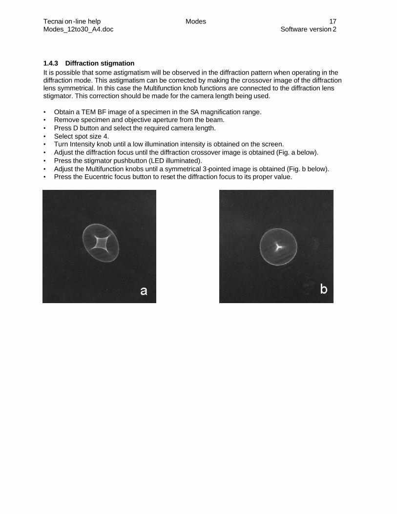
1.4.3 Diffraction stigmation It is possible that some astigmatism will be observed in the diffraction pattern when operating in the diffraction mode. This astigmatism can be corrected by making the crossover image of the diffraction lens symmetrical. In this case the Multifunction knob functions are connected to the diffraction lens stigmator. This correction should be made for the camera length being used. • Obtain a TEM BF image of a specimen in the SA magnification range. • Remove specimen and objective aperture from the beam. • Press D button and select the required camera length. • Select spot size 4. • Turn Intensity knob until a low illumination intensity is obtained on the screen. • Adjust the diffraction focus until the diffraction crossover image is obtained (Fig. a below). • Press the stigmator pushbutton (LED illuminated). • Adjust the Multifunction knobs until a symmetrical 3-pointed image is obtained (Fig. b below). • Press the Eucentric focus button to reset the diffraction focus to its proper value.
Tecnai on -line help Modes 18 Modes_12to30_A4.doc Software version 2
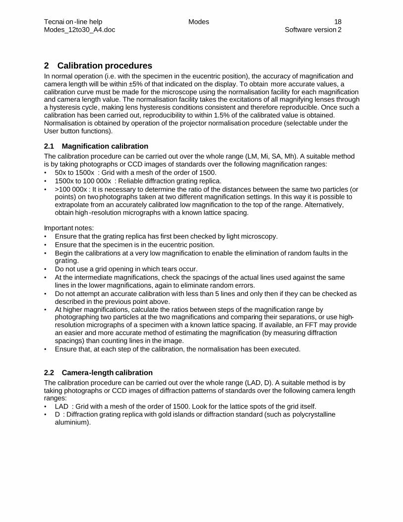
2 Calibration procedures In normal operation (i.e. with the specimen in the eucentric position), the accuracy of magnification and camera length will be within ±5% of that indicated on the display. To obtain more accurate values, a calibration curve must be made for the microscope using the normalisation facility for each magnification and camera length value. The normalisation facility takes the excitations of all magnifying lenses through a hysteresis cycle, making lens hysteresis conditions consistent and therefore reproducible. Once such a calibration has been carried out, reproducibility to within 1.5% of the calibrated value is obtained. Normalisation is obtained by operation of the projector normalisation procedure (selectable under the User button functions).
2.1 Magnification calibration The calibration procedure can be carried out over the whole range (LM, Mi, SA, Mh). A suitable method is by taking photographs or CCD images of standards over the following magnification ranges: • 50x to 1500x : Grid with a mesh of the order of 1500. • 1500x to 100 000x : Reliable diffraction grating replica. • >100 000x : It is necessary to determine the ratio of the distances between the same two particles (or
points) on two photographs taken at two different magnification settings. In this way it is possible to extrapolate from an accurately calibrated low magnification to the top of the range. Alternatively, obtain high -resolution micrographs with a known lattice spacing.
Important notes: • Ensure that the grating replica has first been checked by light microscopy. • Ensure that the specimen is in the eucentric position. • Begin the calibrations at a very low magnification to enable the elimination of random faults in the
grating. • Do not use a grid opening in which tears occur. • At the intermediate magnifications, check the spacings of the actual lines used against the same
lines in the lower magnifications, again to eliminate random errors. • Do not attempt an accurate calibration with less than 5 lines and only then if they can be checked as
described in the previous point above. • At higher magnifications, calculate the ratios between steps of the magnification range by
photographing two particles at the two magnifications and comparing their separations, or use high-resolution micrographs of a specimen with a known lattice spacing. If available, an FFT may provide an easier and more accurate method of estimating the magnification (by measuring diffraction spacings) than counting lines in the image.
• Ensure that, at each step of the calibration, the normalisation has been executed.
2.2 Camera-length calibration The calibration procedure can be carried out over the whole range (LAD, D). A suitable method is by taking photographs or CCD images of diffraction patterns of standards over the following camera length ranges: • LAD : Grid with a mesh of the order of 1500. Look for the lattice spots of the grid itself. • D : Diffraction grating replica with gold islands or diffraction standard (such as polycrystalline
aluminium).

Tecnai on -line help Modes 19 Modes_12to30_A4.doc Software version 2
2.3 Image-diffraction rotation angle The rotation-free series of the Tecnai microscopes result for the majority of magnification and camera lengths in a fixed rotation angle between image and diffraction (dependent on the type of objective lens). The rotation angle is typically not zero (because that would result in a very restricted set of camera lengths available) but 60 or 90°. There may be a few camera lengths and images that do rotate (once again to make these available), typically at the extremes of magnification- and camera-length ranges (especially for energy-filter series). Calibration of the image-diffraction rotation angle can be done by exposure of images and diffraction patterns. A good test specimen for this is molybdenum trioxide crystals on a carbon film. Molybdenum trioxide is (pseudo)orthorhombic with lattice parameters a 0.397 nm, b 1.385 nm and c 0.370 nm. It forms flat crystals, usually lying on [010] that are commonly elongated with the long edges parallel to [001]. From a double-exposure (or overlay) of image and diffraction pattern the rotation angle can be established. To check for 180° inversion, make the diffraction pattern from a relatively thick crystal near one of the points. In the diffraction pattern diffuse intensity will show an 'image' of this point (with the intensities of the diffraction spots also outlining the point. From the direction of the point, it can then be seen whether there is 180° inversion or not.

Tecnai on -line help Modes 20 Modes_12to30_A4.doc Software version 2
3 Bright-field imaging
3.1 Standard method Bright-field imaging is the standard method for the TEM. It simply means making an image with the transmitted beam only. To do so, switch to diffraction and insert and center the objective aperture around the transmitted beam. The aperture selected should be small enough to block all diffracted beams on crystalline specimens. On non -crystalline (biological) specimens, the size of the aperture determines the contrast (smaller apertures give better contrast).
3.2 Working with magnetic specimens The field from magnetic specimens affects the field of the objective lens itself. There are a number of consequences: • The rotation center (beam tilt) is affected by specimen position and tilt. • The beam and image astigmatism is affected by specimen position and tilt. • The beam position may be affected by specimen tilt (often flopping around abruptly when the tilt goes
through 0°). In STEM this may have the result that it is impossible to obtain a normal image (strong distortions).
It should be noted that the microscope is equ ipped with a objective stigmator with a large enough range to allow astigmatism correction of even quite strongly magnetic specimens. The astigmatism correction comes at a price, however. Because the stigmator is not located at the level where the astigmatism is caused (this would be impossible to do construction-wise), the astigmatism correction results in a distortion of the image (one direction is shortened relative to another). This effect is readily observed in high-resolution images (especially of polycrystalline specimens, where the diffraction rings become elliptical). Note: Never use the single-tilt holder with magnetic specimens. The objective-lens field is strong enough to rip the specimen out from underneath the clip and leave it stuck on a pole piece.
3.2.1 Counteracting the magnetism of the specimen In general, prevention is better than a cure and it always pays in convenience and often image quality to spend extra attention in specimen preparation to minimize the actual amount of magnetic material introduced into the microscope (e.g. grind metal disks to a small thickness before jet-polishing so as to keep the amount of material small and keep the disk symmetric, or cut smaller disks (1 to 1.5 mm) and glue them on copper rings). Because of the strong variability of the rotation center with magnetic specimens, it is often easier to use the dark-field tilt to align the rotation center. The following procedure provides a rapid method that leaves the normal microscope alignment unaffected. • With a normal (non-magnetic) specimen set the rotation center. • Switch to diffraction for a selected camera length (e.g. the one closest to 500mm). • Use the normalisation function and accurately center the diffraction pattern on the screen. • Insert the magnetic specimen. • Find a suitable area to start working. • Switch to diffraction, select the same camera length as before and use the normalisation function. • Switch on the dark-field tilt (press the Dark field button) and use the Multifunction knobs to center the
diffraction pattern on the screen. • The incident beam is now parallel to the rotation center without the magnetic specimen. Insert and
center the objective aperture around the beam and go back to imaging. Stay in dark field! • Whenever significant stage-position changes are made, check the beam tilt in diffraction again.

Tecnai on -line help Modes 21 Modes_12to30_A4.doc Software version 2
3.2.2 Lorenz microscopy In the microscope it is also possible to observe the magnetic structure of the specimen. In order to do so (in a microscope not equipped with the special Lorenz lens) execute the following before inserting the specimen into the microscope (otherwise the magnetic structure may be changed or even damaged beyond recovery by the objective -lens field): • Switch the microscope to the LM magnification range. • Switch to diffraction (LAD). • Turn the Focus knob anti-clockwise until it beeps (this sets the objective-lens current to zero). • If necessary, go to the HM-Beam alignment procedure and switch the Minicondenser lens (display its
setting in the status display and turn the lens setting to zero). The Minicondenser lens has a small leak field into the objective -lens gap.
• Insert the specimen holder (not the single-tilt holder!) with the specimen. • Find a suitable area of the specimen and go under- or overfocus. The magnetic structure of the
specimen will now become visible as bright and dark lines. • Make sure you stay in the LM magnification range.
4 Dark-field imaging Dark-field imaging means that the image is made by allowing one (or more) diffracted beams through the objective aperture and blocking the transmitted beam. The advantage of the dark-field image is its inherent high and diffraction -selective contrast.
The origin of the high contrast is shown schematically in the figure to the left. Bright-field as well as dark-field images display changes in intensity across the image. In both cases the total range of intensities is roughly similar. In bright-field images, however, the changes in intensity come on top of a high and unvarying signal – the undiffracted electrons. If one attempts to expose for a longer time to improve the signal, the negative becomes overexposed. In the case of the dark-field the background signal is much lower, leading to a much higher contrast in the image.
Note: With negatives the inherent lower contrast of the bright-field image is inescapable. With slow-scan CCD images it is however possible to subtract the uniform background from the image and stretch the contrast. Two different methods can be used for dark field imaging: 1. Off-axis imaging by aligning the objective apertu re around the diffraction spot of interest. 2. Axial dark field imaging by tilting the incident beam so that the diffracted beam passes through the
objective aperture along the microscope axis. The axial dark field method is preferred because of the higher image quality obtained with on-axis imaging and ease of use through simple change-over between bright field and dark field.
4.1 Axial dark-field imaging Before activating dark field, execute the following procedure: • Center the beam. • Press Dark-field while in T EM mode in the SA magnification range. • Set the dark-field tilts to 0.00 by pressing Reset. The corresponding dark field beam shift (a value
relative to the bright-field beam shift) will also be set to zero.

Tecnai on -line help Modes 22 Modes_12to30_A4.doc Software version 2
Obtaining a dark field image: • In TEM BF mode, select required field of view in the SA magnification range. • Obtain a diffraction pattern of the chosen area. • Center the diffraction pattern on the screen with the diffraction shift. • Decide from which Bragg reflection (or section of a polycrystalline ring) a dark field image is to be
obtained. • Press the Dark-field button (green LED on). • Use Multifunction X and Y knobs to bring the Bragg reflection opposite to the one selected to the
point where the central beam was originally positioned (this should be the center of the screen). • Key Dark-field to return to Bright Field Diffraction mode. • Introduce an objective aperture and center it accurately around the central spot. • Key Dark-field to return to Dark Field Diffraction mode. • Center the chosen diffraction spot accurately in the objective aperture using the Multifunction X and
Y knobs. The objective aperture must be small enough to isolate the chosen spot from neighbouring diffracted beams.
• Press D button (LED off) and a dark field image of those crystal planes causing the selected diffraction spot will now appear.
• Carry out Magnification, Intensity, beam Shift and Focus adjustments as for a Bright Field image. Switching between Dark and Bright Field images may be achieved simply by successively pressing the Dark-field button. Multiple settings for different dark-field tilts can be stored in the dark-field channels.
4.2 Off-axis imaging Procedure • Switch to diffraction. • Center the objective aperture around the diffracted beam required for dark-field imaging. • Switch back to imaging.
Tecnai on -line help Modes 23 Modes_12to30_A4.doc Software version 2
5 Diffraction
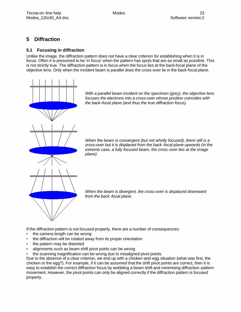
5.1 Focusing in diffraction Unlike the image, the diffraction pattern does not have a clear criterion for establishing when it is in focus. Often it is presumed to be 'in focus' when the pattern has spots that are as small as possible. This is not strictly true. The diffraction pattern is in focus when the focus lies at the back-focal plane of the objective lens. Only when the incident beam is parallel does the cross-over lie in the back-focal plane.
With a parallel beam incident on the specimen (grey), the objective lens focuses the electrons into a cross-over whose position coincides with the back-focal plane (and thus the true diffraction focus). When the beam is convergent (but not wholly focused), there still is a cross-over but it is displaced from the back -focal plane upwards (in the extreme case, a fully focused beam, the cross-over lies at the image plane). When the beam is divergent, the cross-over is displaced downward from the back -focal plane.
If the diffraction pattern is not focused properly, there are a number of consequences: • the camera length can be wrong • the diffraction will be rotated away from its proper orientation • the pattern may be distorted • alignments such as beam shift pivot points can be wrong • the scanning magnification can be wrong due to misaligned pivot points Due to the absence of a clear criterion, we end up with a chicken -and-egg situation (what was first, the chicken or the egg?). For example, if it can be assumed that the shift pivot points are correct, then it is easy to establish the correct diffraction focus by wobbling a beam shift and minimising diffraction -pattern movement. However, the pivot points can only be aligned correctly if the diffraction pattern is focused properly.
Tecnai on -line help Modes 24 Modes_12to30_A4.doc Software version 2
In order to resolve this situation, we have determined Intensity settings for the different modes (LM, HM-TEM and Nanoprobe) for a parallel beam. These Intensity settings are preset in the alignment procedures, making it easy to find diffraction focus (the spot-pattern condition). After the alignment have been done (camera length focus), the diffraction focus can also be found by simply pressing the Eucentric focus button (this resets the variable diffraction focus to zero). With this method for establishing diffraction focus, the SA aperture is not (and should not be) used.
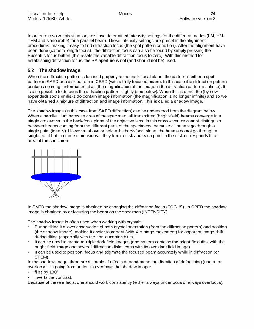
5.2 The shadow image When the diffraction pattern is focused properly at the back-focal plane, the pattern is either a spot pattern in SAED or a disk pattern in CBED (with a fu lly focused beam). In this case the diffraction pattern contains no image information at all (the magnification of the image in the diffraction pattern is infinite). It is also possible to defocus the diffraction pattern slightly (see below). When this is done, the (by now expanded) spots or disks do contain image information (the magnification is no longer infinite) and so we have obtained a mixture of diffraction and image information. This is called a shadow image. The shadow image (in this case from SAED diffraction) can be understood from the diagram below. When a parallel illuminates an area of the specimen, all transmitted (bright-field) beams converge in a single cross-over in the back-focal plane of the objective lens. In this cross-over we cannot distinguish between beams coming from the different parts of the specimens, because all beams go through a single point (ideally). However, above or below the back-focal plane, the beams do not go through a single point but - in three dimensions - they form a disk and each point in the disk corresponds to an area of the specimen.
In SAED the shadow image is obtained by changing the diffraction focus (FOCUS). In CBED the shadow image is obtained by defocusing the beam on the specimen (INTENSITY). The shadow image is often used when working with crystals : • During tilting it allows observation of both crystal orientation (from the diffraction pattern) and position
(the shadow image), making it easier to correct (with X-Y stage movement) for apparent image shift during tilting (especially with the non -eucentric b tilt).
• It can be used to create multiple dark-field images (one pattern contains the bright-field disk with the bright-field image and several diffraction disks, each with its own dark-field image).
• It can be used to position, focus and stigmate the focused beam accurately while in diffraction (or STEM).
In the shadow image, there are a couple of effects dependent on the direction of defocusing (under- or overfocus). In going from under- to overfocus the shadow image: • flips by 180°. • inverts the contrast. Because of these effects, one should work consistently (either always underfocus or always overfocus).
Tecnai on -line help Modes 25 Modes_12to30_A4.doc Software version 2
5.3 Selected-area diffraction Selected-area diffraction has been the main diffraction technique for a long time. However, since the introduction of instruments capable of illuminating areas of nanometer-size, convergent-beam (or with a somewhat defocused or even parallel beam, aperture-less) diffraction has gained in importance. One reason is the resolution limitation of selected -area diffraction (see the nomogram below). Another reason is the difficulty of judging whether –g and +g beams are of equal intensities (and the orientation is thus in a symmetrical condition), which is especially important for high -resolution imaging.
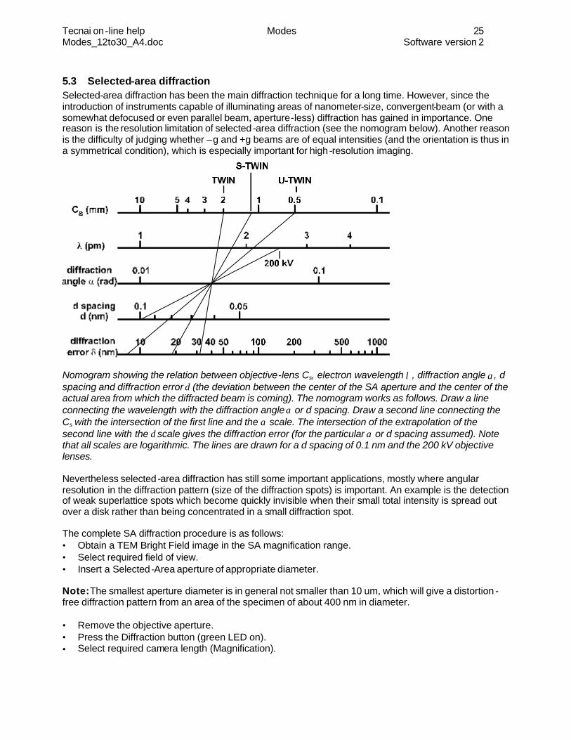
Nomogram showing the relation between objective-lens Cs, electron wavelength λ , diffraction angle α, d spacing and diffraction error δ (the deviation between the center of the SA aperture and the center of the actual area from which the diffracted beam is coming). The nomogram works as follows. Draw a line connecting the wavelength with the diffraction angle α or d spacing. Draw a second line connecting the Cs with the intersection of the first line and the α scale. The intersection of the extrapolation of the second line with the δ scale gives the diffraction error (for the particular α or d spacing assumed). Note that all scales are logarithmic. The lines are drawn for a d spacing of 0.1 nm and the 200 kV objective lenses. Nevertheless selected -area diffraction has still some important applications, mostly where angular resolution in the diffraction pattern (size of the diffraction spots) is important. An example is the detection of weak superlattice spots which become quickly invisible when their small total intensity is spread out over a disk rather than being concentrated in a small diffraction spot. The complete SA diffraction procedure is as follows: • Obtain a TEM Bright Field image in the SA magnification range. • Select required field of view. • Insert a Selected -Area aperture of appropriate diameter. Note: The smallest aperture diameter is in general not smaller than 10 um, which will give a distortion -free diffraction pattern from an area of the specimen of about 400 nm in diameter. • Remove the objective aperture. • Press the Diffraction button (green LED on). • Select required camera length (Magnification).
Tecnai on -line help Modes 26 Modes_12to30_A4.doc Software version 2
• Focus the diffraction pattern. • Adjust Intensity of illumination to a suitable level by turning clockwise to reduce the intensity. • Refocus the diffraction pattern if necessary. Note: Recording the diffraction pattern should be carried out with manual exposure-time selection as automatic exposure readings are not reliable in the diffraction mode. The time is best judged from experience gained from a series of test exposures obtained with fixed illumination conditions (emission, high tension, intensity and spot size) for the different sizes of selected -area apertures. As a rough estimate, one-third of the value of the automatic exposure time may be used.
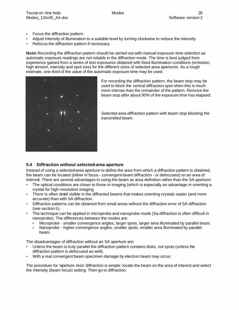
For recording the diffraction pattern, the beam stop may be used to block the central diffraction spot when this is much more intense than the remainder of the pattern. Remove the beam stop after about 90% of the exposure time has elapsed. Selected area diffraction pattern with beam stop blocking the transmitted beam.
5.4 Diffraction without selected-area aperture Instead of using a selected-area aperture to define the area from which a diffraction pattern is obtained, the beam can be located (either in focus - convergent-beam diffraction - or defocused) on an area of interest. There are several advantages to using the beam as area definition rather than the SA aperture: • The optical conditions are closer to those in imaging (which is especially an advantage in orienting a
crystal for high-resolution imaging. • There is often detail visible in the diffracted beams that makes orienting crystals easier (and more
accurate) than with SA diffraction. • Diffraction patterns can be obtained from small areas without the diffraction error of SA diffraction
(see section 5). • The technique can be applied in microprobe and nanoprobe mode (Sa diffraction is often difficult in
nanoprobe). The differences between the modes are: • Microprobe - smaller convergence angles, larger spots, larger area illuminated by parallel beam. • Nanoprobe - higher convergence angles, smaller spots, smaller area illuminated by parallel
beam. The disadvantages of diffraction without an SA aperture are: • Unless the beam is truly parallel the diffraction pattern contains disks, not spots (unless the
diffraction pattern is defocused as well). • With a real convergent beam specimen damage by electron beam may occur. The procedure for 'aperture -less' diffraction is simple: locate the beam on the area of interest and select the Intensity (beam focus) setting. Then go to diffraction.
Tecnai on -line help Modes 27 Modes_12to30_A4.doc Software version 2
5.5 Standard convergent-beam diffraction For 'real' convergent-beam diffraction, the beam is simply focused on the specimen. Typical convergent beam diffraction conditions can be either the microprobe or nanoprobe mode, spot size s in the smaller spot size range (> spot 5), condenser aperture dependent on the diffraction angle required (which is usually determined by the smallest spacing between the diffracted beams for the crystal orientation of interest). The convergent-beam pattern consists of two types of features: 1. The diffraction disks which essentially are images of the condenser aperture. 2. The diffraction information inside the disks. These two types of features react differently to different types of manipulation: 1. The position of the diffraction disks depends on de tilt angle of the incident beam (a tilt in the image is
a shift in diffraction). The position can be changed by either shifting the condenser aperture or tilting the beam itself (dark field). Changing the position of the disks does not affect the overall position of the diffraction information (which behaves like a background over which the aperture images appear to move).
2. The position of the diffraction information depends on the orientation of the crystal. Tilting the crystal thus moves the pattern of diffraction information but leaves the position of the disk unaffected.
These characteristics can be used for fine-tuning of the convergent-beam pattern.
5.5.1 Orienting the crystal In order to minimize distortions of the beam, any fine -tuning (as described below) should be limited to small angles. It is therefore important to make sure the specimen is as well-oriented as can be achieved with the α and β tilts of the specimen holder. It will be seen that the diffraction disks of the CBED pattern stay in position while tilting and that it is the structure inside the disks that moves. Make the pattern as symmetrical as possible by tilting.
5.5.2 Fine-tuning pattern Once the crystal has been oriented as well as possible with the mechanical stage tilts, there are two methods for fine-tuning the pattern. Since the CBED pattern is a reflection of the relative orientation of the crystal and the beam, tilting the crystal and beam have the same effect (except that tilted beams become distorted due to electron -optical aberrations). Tilting the beam is often easier in the end stages of preparing CBED pattern because finer control is possible. Tilting can be achieved in two ways, one using the dark-field tilt (preferred method since it can be reset very easily), the other by moving the condenser aperture.
5.6 Large-angle convergent beam (LACBED/Tanaka) Convergent beam diffraction patterns (CBED) can provide a wealth of information about the crystallography of a specimen. The amount of information available depends on the size of the disks in the CBED pattern, which is limited by the spacing of the disks, since disks are not allowed to overlap (except in coherent CBED, a technique limited to FEG instruments). Even for structures with fairly normal-sized unit cells the disk size on zone axes with low indices is usually small so that only a limited amount of information is obtainable. In many instances, e.g. for the determina tion of the presence or absence of an inversion center, more information in larger disks is required. This information can be obtained by using the Large -Angle Convergent Beam (LACBED) or Tanaka technique. With this technique, larger convergence angle (and hence large disks) can be obtained without overlap between adjacent disks. This result is obtained by moving the specimen out of the plane of focus (or moving the

Tecnai on -line help Modes 28 Modes_12to30_A4.doc Software version 2
focus out of the specimen plane) while keeping the beam focused. When this is done, a diffraction pattern appears overlaid on the image, with the size of the diffraction pattern proportional to the distance between the specimen and the focus plane. The selected area aperture can then be used to select a single beam, either the transmitted beam or a diffracted beam, which is then the only beam contributing to the diffraction pattern. Procedure • Start in the TEM (microprobe) mode. Center the specimen at the eucentric height. Orient the
specimen as required. • Set up the nanoprobe mode with a condenser aperture of 50 um, with beam centered and focused,
and the image in focus. Select a spot size somewhere in the low end of the range (higher spot numbers). Check that the specimen orientation is still in the proper orientation. If high angles are required, increase the size of the condenser aperture.
• Increase the focus (typically by several micrometers) or alternatively move the specimen up with the Z axis height control (the advantage of moving the specimen is that the electron-optical conditions do not change; the disadvantage that the specimen is moved and is no longer eucentric).
• A diffraction pattern will now be visible around the transmitted beam. • Insert a selected -area aperture (start with the smallest) around the transmitted beam. If the aperture
is still too large so that diffracted beams still pass through the aperture, increase the focus current/raise the specimen further.
• Once the diffraction pattern is large enough to allow only one beam to pass through it, center the aperture around the beam of choice (transmitted or diffracted).
• Switch to diffraction and you have the LACBED pattern. Notes: • The maximum diffraction angle is determined by the size of the condenser aperture, the objective-
lens current (the highest angle is typically obtained for objective -lens settings of 5 to 10 um overfocus) and the SA aperture. It is easy to establish if the condenser or SA aperture is angle-limiting. Simply shift one of the apertures slightly. If the shadow at the edge of the diffraction disk moves with it, that is the limiting aperture. If the condenser aperture is angle-limiting (and higher angles are needed), switch to a larger aperture if possible. If it is the SA aperture, switch to a larger SA aperture but remember to check that the aperture allows only one beam to pass!
• A properly focused beam will typically have a small bright spot in the center, surrounded by a halo (caused by the spherical aberration of the objective lens).
• Optimize the diffraction angle by slightly changing the Intensity setting to get the largest disk size and at the same time not running against the SA aperture.
• If ‘sausage’-shaped dark areas are visible in the pattern, the beam is not properly centered inside the SA aperture.
One problem with LACBED patterns is that they mix diffraction and image information because the interaction area between the specimen and beam is large (the beam is focused but not at the specimen itself). This is the price one pays for having no overlap and yet large disks. Because of the mix of image and diffraction information, LACBED patterns often display distortions (due to specimen bending) and thickness changes across the disk. Another ‘feature’ of LACBED patterns is that they show rubbish on the specimen surface with high contrast (but often only visible once the negatives have been recorded). Make sure the specimen is as clean as you can get it. It is also possible to have simultaneous bright-field (transmitted-beam) and dark-field (diffracted) beams in single pattern. To achieve that do not insert an SA aperture but stay in image mode and defocus the beam (Intensity) until the beams of the diffraction pattern touch each other.
Tecnai on -line help Modes 29 Modes_12to30_A4.doc Software version 2
6 Analysis There is a big difference between EDX and EELS analysis. In the case of EDX analysis, the detector is mounted close to the specimen and X-rays can be detected from the whole specimen area, not only the area intended (and hit by a focused beam). In the case of EELS it is much easier to keep 'spurious' signals out from the detector. For EDX it is important therefore to pay attention to the conditions for analysis.
6.1 EDX analysis Because of the location of the detector, EDX analysis is sensitive to 'spurious' signals, that is, signals generated outside the focused electron beam and thus outside the area of interest. These signals can in principle come from a specimen-mounting grid, specimen holder, objective aperture and objective-lens pole pieces. Some of these effects can be partially avoided by paying attention to the analysis conditions, but some spurious signals will always exist (for example from electrons backscattered from the specimen area which then hit other areas of the specimen again).
6.1.1 Microprobe versus nanoprobe The electron optics of the column with regard to the two modes result in a large field of view in the microprobe mode (with the beam able to illuminate a wide area) whereas in the nanoprobe mode the beam cannot be defocused further than several micrometers. Stray electrons (scattered at the edge of apertures) can only occur within the area that can be illuminated by the beam. In nanoprobe any stray electrons are therefore confined to a few micrometers around the electron beam itself. Especially in ion-milled or jet-polished specimens, the stray electrons therefore strike only thin parts of the specimen and thus do not have a significant effect on the EDX spectrum (which in principle should contain only information from the area within the beam itself). In the microprobe mode, the stray electrons can strike the specimen over a much larger area, including thick areas where a single incident electron can generate up to tens of X rays. The nanoprobe mode is therefore better suited for EDX analysis.
6.1.2 Shadowing angle The EDX detector is mounted at a finite angle above the plane of the specimen, typically somewhere between 10 and 20°. This has consequences, not only for absorption (at lower angles the path of the X rays through the specimen is longer) but also for the 'visibility' of the specimen. In fact, the angle listed for detectors is somewhat 'cosmetic' because it refers to the angle through the heart of the detector crystal. In practice this can mean that the lower edge of the detector crystal is only slightly above (or even below) 0°. For good analysis the specimen must therefore be tilted. The amount of tilt required depends to some extent on the specimen position (the Y axis, especially when the value is strongly negative) and specimen itself (Focused Ion Beam - FIB - specimens must be mounted so they face the detector), but mostly it is the detector configuration itself. The angle at which shadowing stops can be determined by collecting EDX spectra at various tilt angles (0, 5, 10, …) and comparing the count rates for these angles (note that there is of course a change in effective specimen thickness as the tilt angle goes away from 0°). Find the tilt angle where the increase in count rate to higher tilt angles levels off and use that (with a margin of an additional 5°) as the minimum tilt angle used for EDX analysis. Note: Never use a normal holder for EDX analysis. Special low-background holders with beryllium shielding around the specimen exist in single -tilt and double -tilt versions. Some of the regular holders (especially the single tilt) also have very 'deep' specimen cups and completely shield the specimen from the EDX detector unless the tilt angle is well above 25°.
Tecnai on -line help Modes 30 Modes_12to30_A4.doc Software version 2
6.2 EELS analysis EELS analysis can be done in two modes, image mode and diffraction mode. In image mode, the projection-system cross-over, which is imaged again on the EELS spectrometer as a spectrum is a diffraction pattern (this means that the spectrum is a diffraction pattern at the same time). This mode is therefore called diffraction coupling. Conversely, in diffraction, the cross-over contains an image, and this is called image-coupling. The size of the cross-over (and thus to some extent the resolution of the spectrum) is inversely related to the magnification or camera length. There is a second factor related to the diffraction- or image-coupling. The standard mode of operation for EELS analysis is diffraction (image coupling). The diffraction pattern is simply placed at the entrance aperture of the PEELS or Imaging Filter. Area selection is done with the focused beam. One reason for using diffraction is that one can simply move from one area for analysis to another by shifting the beam; the diffraction pattern will remain stationary and so it is not necessary to center the beam on the EELS entrance aperture. This same principle applies to analysis in STEM. It should be realized, however, that the beam shifts (in one direction; the other direction is parallel to the energy axis of the spectrum) will be visible in the spectrum as a spectrum shift. This effect gets magnified at low camera lengths (as often used for EELS). The effect is readily visible when EELS spectrum acquisition is done in STEM with a continuously scanning beam at low camera length. Under these conditions the apparent energy resolution may be 10 eV or more. For proper operation under such conditions a descan facility is needed (but not yet available on Tecnai).
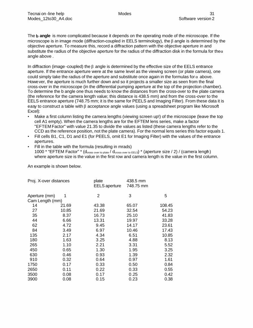
6.2.1 Determining spectrometer acceptance angle β An important parameter in EELS quantification of the spectrometer acceptance half-angle β . (Another parameter, the beam convergence angle α is also important in the sense that it should be less than β, but most users have less problems with determining α than β). The α angle can be measured simply from a diffraction pattern. The equations can be derived as follows: Bragg's Law 2θB = λ / d where 2θB is the Bragg angle, λ the electron wavelength and d the d spacing. Camera constant D d = L λ where L is the camera length and D the distance between transmitted and diffracted beam in the recorded diffraction pattern. CBED α / 2θB = A / D The latter formula says that the angles in the diffraction pattern (convergence angle and a Bragg angle of a diffracted beam) are proportional to the ratio between the distances measured in the pattern (the radius of the diffraction disk A and the distance from transmitted to diffracted beam D). These formulas can be converted to: α = A 2 θB / D (a rewriting of the CBED formula) or α = A / L
Tecnai on -line help Modes 31 Modes_12to30_A4.doc Software version 2
The β angle is more complicated because it depends on the operating mode of the microscope. If the microscope is in image mode (diffraction-coupled in EELS terminology), the β angle is determined by the objective aperture. To measure this, record a diffraction pattern with the objective aperture in and substitute the radius of the objective aperture for the radius of the diffraction disk in the formula for the α angle above . In diffraction (image-coupled) the β angle is determined by the effective size of the EELS entrance aperture. If the entrance aperture were at the same level as the viewing screen (or plate camera), one could simply take the radius of the aperture and substitute once again in the formulas for α above. However, the aperture is much further down and so it projects a smaller size as seen from the final cross-over in the microscope (in the differential pumping aperture at the top of the projection chamber). To determine the b angle one thus needs to know the distances from the cross-over to the plate camera (the reference for the camera length value; this distance is 438.5 mm) and from the cross-over to the EELS entrance aperture (748.75 mm; it is the same for PEELS and Imaging Filter). From these data it is easy to construct a table with β acceptance angle values (using a spreadsheet program like Microsoft Excel): • Make a first column listing the camera lengths (viewing screen up!) of the microscope (leave the top
cell A1 empty). When the camera lengths are for the EFTEM lens series, make a factor "EFTEM Factor" with value 21.35 to divide the values as listed (these camera lengths refer to the CCD as the reference position, not the plate camera). For the normal lens series this factor equals 1.
• Fill cells B1, C1, D1 and E1 (for PEELS, omit E1 for Imaging Filter) with the values of the entrance apertures.
• Fill in the table with the formula (resulting in mrads) 1000 * “EFTEM Factor” * (dcross- over to plate / dcross- over to EELS) * (aperture size / 2) / (camera length) where aperture size is the value in the first row and camera length is the value in the first column.
An example is shown below. Proj. X-over distances plate 438.5 mm EELS aperture 748.75 mm Aperture (mm) 1 2 3 5 Cam Length (mm) 14 21.69 43.38 65.07 108.45 27 10.85 21.69 32.54 54.23 35 8.37 16.73 25.10 41.83 44 6.66 13.31 19.97 33.28 62 4.72 9.45 14.17 23.61 84 3.49 6.97 10.46 17.43 135 2.17 4.34 6.51 10.85 180 1.63 3.25 4.88 8.13 265 1.10 2.21 3.31 5.52 450 0.65 1.30 1.95 3.25 630 0.46 0.93 1.39 2.32 910 0.32 0.64 0.97 1.61 1750 0.17 0.33 0.50 0.84 2650 0.11 0.22 0.33 0.55 3500 0.08 0.17 0.25 0.42 3900 0.08 0.15 0.23 0.38

Tecnai on -line help Modes 32 Modes_12to30_A4.doc Software version 2
7 STEM In the STEM (or Scanning) mode of the microscope images are acquired by moving a focused beam in a raster across the specimen and collecting a signal at each x,y pixel coordinates. The signals for all pixels together make the STEM image.
7.1 STEM principles When a focused beam is moved across a specimen, the signals generated by the interaction between the electron beam and the specimen will vary according to specimen characteristics such as material type (composition and structure), orientation (diffraction from crystals), and topography. When the beam is scanned across the specimen in a rectangular raster, the change in signals allows one to build up an image of the specimen. The scanning of the beam across the specimen on the Tecnai microscope is achieved through a set of beam deflection coils (called the AC coils) that is separate from the 'static' beam shift coils (or DC coils). The AC beam deflection of the scan is thus superimposed on the DC deflection (which is used to align the beam along the optical axis - the rotation center - and center the beam). The AC deflection coils have their own characteristics and thus their own pivot points, separate from those of the DC coils (the procedure to align the AC coils is similar to the DC alignment, though). STEM magnification works different from TEM magnification. The TEM magnification is the result of the magnification by the objective lens (a constant value) and the - variable - lenses of the projector system (Diffraction, Intermediate, Projector lenses). The STEM magnification is the result of the deflection of the beam. If the beam is deflected far from the optical axis, the scanned area is large and thus the STEM magnification low. When the beam is deflected only a little, the scanned area is small and the STEM magnification high. Some STEM detectors are located close to the specimen (secondary-electron, backscattered electron) and for these the setup of the magnification system is irrelevant (they would still work even if the microscope shutter - below the specimen area - would be closed). For other detectors, like the bright-field and dark-field detectors, the setup of the magnification system is important. The setup of the bright-field/dark-field detectors makes clever use of a characteristic of a beam that is being scanned parallel to the optical axis: the diffraction pattern remains stationary while the beam moves. It is therefore possible to detect the bright-field signal by placing the central (transmitted) beam on a bright-field detector, while an annular (ring-shaped) dark-field detector around the bright-field collects the signal from (some of) the diffracted beams. Which diffracted beams (or rather, which range of diffraction angles) are being collected on the dark-field detector depends on the camera length of the diffraction pattern. At low camera lengths the collected angles are large (and the dark-field detector effectively is a high-angle annular dark-field detector), while at higher camera lengths the angles are smaller. The limitation on camera lengths on the lower side is determined by the off-axis diffraction shift required to move the diffraction pattern to the detector (the bright-field/dark-field detectors are located about 3 cm away from the center of the viewing screen), while on the high side the limitation (in this case only for dark-field) is the size of the diffraction disk of the central beam (since the beam is focused, the diffraction pattern has disks, not spots). Once the central-beam disk becomes too large, it starts to fall on the dark-field detector. There are typically two camera lengths around 90 to 100mm. One of these is rotation-free, the other is not (it is rotated relative to the other camera lengths). The rotated camera length is used for STEM high-angle dark-field imaging with the normal dark-field detector (on the lowermost rotation-free camera lengths the high diffraction angles are shadowed by the differential pumping aperture, so very little high-angle dark-field signal is available).
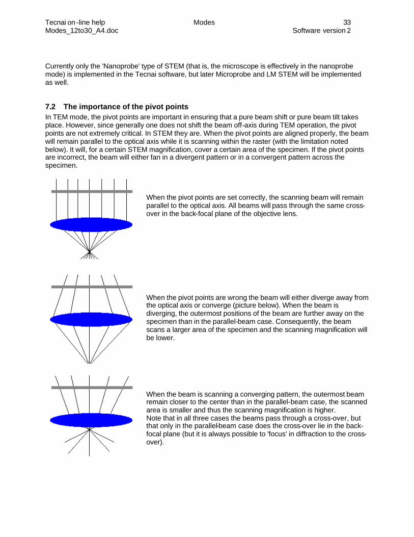
Tecnai on -line help Modes 33 Modes_12to30_A4.doc Software version 2
Currently only the 'Nanoprobe' type of STEM (that is, the microscope is effectively in the nanoprobe mode) is implemented in the Tecnai software, but later Microprobe and LM STEM will be implemented as well.
7.2 The importance of the pivot points In TEM mode, the pivot points are important in ensuring that a pure beam shift or pure beam tilt takes place. However, since generally one does not shift the beam off-axis during TEM operation, the pivot points are not extremely critical. In STEM they are. When the pivot points are aligned properly, the beam will remain parallel to the optical axis while it is scanning within the raster (with the limitation noted below). It will, for a certain STEM magnification, cover a certain area of the specimen. If the pivot points are incorrect, the beam will either fan in a divergent pattern or in a convergent pattern across the specimen.
When the pivot points are set correctly, the scanning beam will remain parallel to the optical axis. All beams will pass through the same cross-over in the back-focal plane of the objective lens.
When the pivot points are wrong the beam will either diverge away from the optical axis or converge (picture below). When the beam is diverging, the outermost positions of the beam are further away on the specimen than in the parallel-beam case. Consequently, the beam scans a larger area of the specimen and the scanning magnification will be lower. When the beam is scanning a converging pattern, the outermost beam remain closer to the center than in the parallel-beam case, the scanned area is smaller and thus the scanning magnification is higher. Note that in all three cases the beams pass through a cross-over, but that only in the parallel-beam case does the cross-over lie in the back-focal plane (but it is always possible to 'focus' in diffraction to the cross-over).
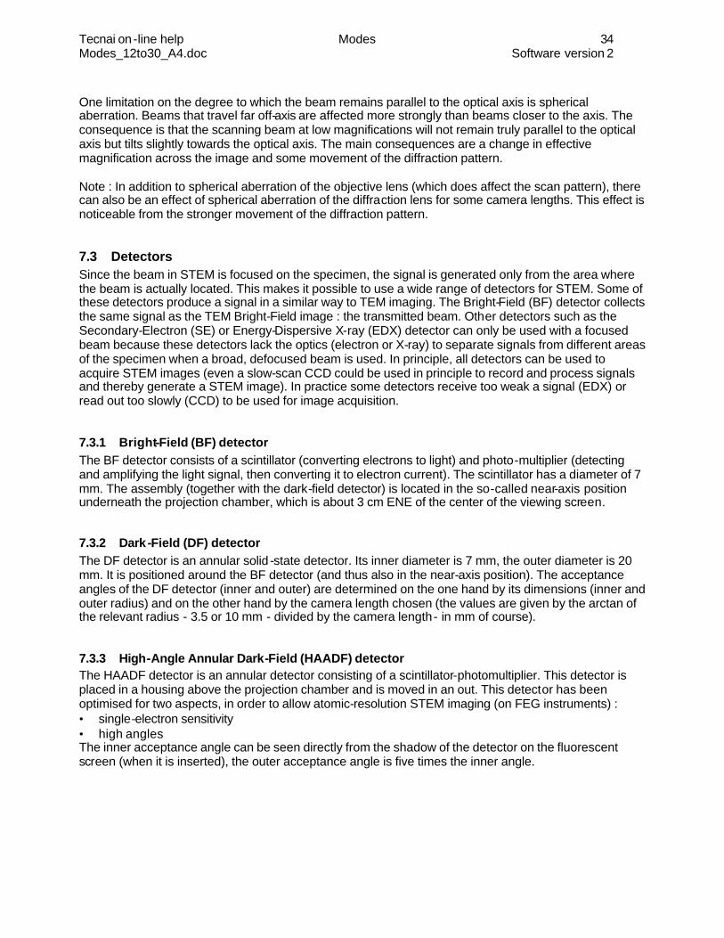
Tecnai on -line help Modes 34 Modes_12to30_A4.doc Software version 2
One limitation on the degree to which the beam remains parallel to the optical axis is spherical aberration. Beams that travel far off-axis are affected more strongly than beams closer to the axis. The consequence is that the scanning beam at low magnifications will not remain truly parallel to the optical axis but tilts slightly towards the optical axis. The main consequences are a change in effective magnification across the image and some movement of the diffraction pattern. Note : In addition to spherical aberration of the objective lens (which does affect the scan pattern), there can also be an effect of spherical aberration of the diffraction lens for some camera lengths. This effect is noticeable from the stronger movement of the diffraction pattern.
7.3 Detectors Since the beam in STEM is focused on the specimen, the signal is generated only from the area where the beam is actually located. This makes it possible to use a wide range of detectors for STEM. Some of these detectors produce a signal in a similar way to TEM imaging. The Bright-Field (BF) detector collects the same signal as the TEM Bright-Field image : the transmitted beam. Other detectors such as the Secondary-Electron (SE) or Energy-Dispersive X-ray (EDX) detector can only be used with a focused beam because these detectors lack the optics (electron or X-ray) to separate signals from different areas of the specimen when a broad, defocused beam is used. In principle, all detectors can be used to acquire STEM images (even a slow-scan CCD could be used in principle to record and process signals and thereby generate a STEM image). In practice some detectors receive too weak a signal (EDX) or read out too slowly (CCD) to be used for image acquisition.
7.3.1 Bright-Field (BF) detector The BF detector consists of a scintillator (converting electrons to light) and photo-multiplier (detecting and amplifying the light signal, then converting it to electron current). The scintillator has a diameter of 7 mm. The assembly (together with the dark-field detector) is located in the so-called near-axis position underneath the projection chamber, which is about 3 cm ENE of the center of the viewing screen.
7.3.2 Dark-Field (DF) detector The DF detector is an annular solid -state detector. Its inner diameter is 7 mm, the outer diameter is 20 mm. It is positioned around the BF detector (and thus also in the near-axis position). The acceptance angles of the DF detector (inner and outer) are determined on the one hand by its dimensions (inner and outer radius) and on the other hand by the camera length chosen (the values are given by the arctan of the relevant radius - 3.5 or 10 mm - divided by the camera length - in mm of course).
7.3.3 High-Angle Annular Dark-Field (HAADF) detector The HAADF detector is an annular detector consisting of a scintillator-photomultiplier. This detector is placed in a housing above the projection chamber and is moved in an out. This detector has been optimised for two aspects, in order to allow atomic-resolution STEM imaging (on FEG instruments) : • single-electron sensitivity • high angles The inner acceptance angle can be seen directly from the shadow of the detector on the fluorescent screen (when it is inserted), the outer acceptance angle is five times the inner angle.
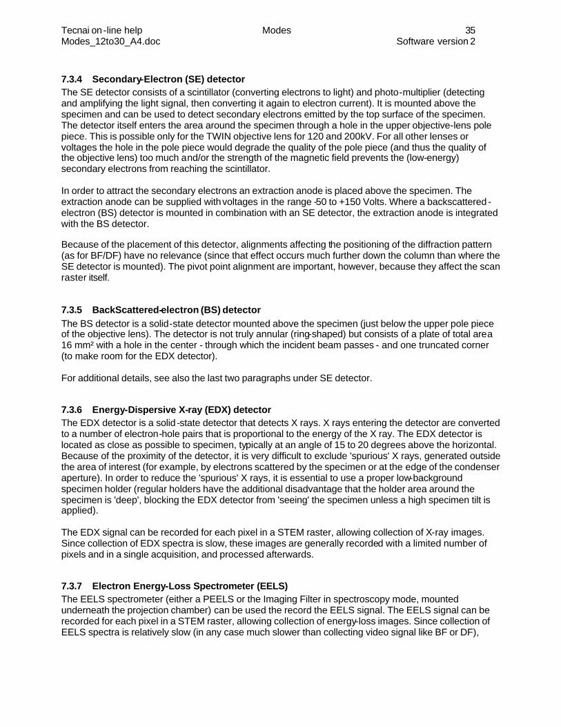
Tecnai on -line help Modes 35 Modes_12to30_A4.doc Software version 2
7.3.4 Secondary-Electron (SE) detector The SE detector consists of a scintillator (converting electrons to light) and photo-multiplier (detecting and amplifying the light signal, then converting it again to electron current). It is mounted above the specimen and can be used to detect secondary electrons emitted by the top surface of the specimen. The detector itself enters the area around the specimen through a hole in the upper objective-lens pole piece. This is possible only for the TWIN objective lens for 120 and 200kV. For all other lenses or voltages the hole in the pole piece would degrade the quality of the pole piece (and thus the quality of the objective lens) too much and/or the strength of the magnetic field prevents the (low-energy) secondary electrons from reaching the scintillator. In order to attract the secondary electrons an extraction anode is placed above the specimen. The extraction anode can be supplied with voltages in the range -50 to +150 Volts. Where a backscattered -electron (BS) detector is mounted in combination with an SE detector, the extraction anode is integrated with the BS detector. Because of the placement of this detector, alignments affecting the positioning of the diffraction pattern (as for BF/DF) have no relevance (since that effect occurs much further down the column than where the SE detector is mounted). The pivot point alignment are important, however, because they affect the scan raster itself.
7.3.5 BackScattered-electron (BS) detector The BS detector is a solid-state detector mounted above the specimen (just below the upper pole piece of the objective lens). The detector is not truly annular (ring-shaped) but consists of a plate of total area 16 mm² with a hole in the center - through which the incident beam passes - and one truncated corner (to make room for the EDX detector). For additional details, see also the last two paragraphs under SE detector.
7.3.6 Energy-Dispersive X-ray (EDX) detector The EDX detector is a solid -state detector that detects X rays. X rays entering the detector are converted to a number of electron-hole pairs that is proportional to the energy of the X ray. The EDX detector is located as close as possible to specimen, typically at an angle of 15 to 20 degrees above the horizontal. Because of the proximity of the detector, it is very difficult to exclude 'spurious' X rays, generated outside the area of interest (for example, by electrons scattered by the specimen or at the edge of the condenser aperture). In order to reduce the 'spurious' X rays, it is essential to use a proper low-background specimen holder (regular holders have the additional disadvantage that the holder area around the specimen is 'deep', blocking the EDX detector from 'seeing' the specimen unless a high specimen tilt is applied). The EDX signal can be recorded for each pixel in a STEM raster, allowing collection of X-ray images. Since collection of EDX spectra is slow, these images are generally recorded with a limited number of pixels and in a single acquisition, and processed afterwards.
7.3.7 Electron Energy-Loss Spectrometer (EELS) The EELS spectrometer (either a PEELS or the Imaging Filter in spectroscopy mode, mounted underneath the projection chamber) can be used the record the EELS signal. The EELS signal can be recorded for each pixel in a STEM raster, allowing collection of energy-loss images. Since collection of EELS spectra is relatively slow (in any case much slower than collecting video signal like BF or DF),

Tecnai on -line help Modes 36 Modes_12to30_A4.doc Software version 2
these images are generally recorded with a limited number of pixels and in a single acquisition, and processed afterwards.
7.4 Detector alignment For proper STEM operation with the BF/DF detectors, the diffraction pattern must be centered correctly on the detectors. In order to make this easier, the microscope has a separate alignment (an additional diffraction shift per camera length) that can be used to switch rapidly between a centered diffraction pattern and a pattern shifted to the detectors. The advantage of the detector alignment is the reproducibility of the off-axis shift. Once the diffraction pattern has been centered on the screen, it is much easier to shift accurately to the detector. Note: The centering of the diffraction pattern on the screen depends on the diffraction shift set as well as on the rotation center. Misalignment of the rotation center (which effectively is a beam tilt) gives a diffraction shift, so check the rotation center as well. In addition, the centering of the diffraction pattern may be sensitive to the magnification-system lens settings. Using projector normalization makes the position much better reproducible.
7.5 STEM adjustments - an in-depth explanation The pivot points are not the only adjustments made to the STEM system. Ideally deflection coils have the following characteristics: • Shifts on the x and y coils keep the beam parallel to the optical axis - implying that the upper-x and
lower-x coils are perfectly matched (and the same for upper-y and lower-y). • The upper and lower coils are perfectly aligned (that is, the is no rotation between the upper and
lower coils). • The x and y coils produce the same amount of shift (the magnetic fields of the coils are equal). • The x and y coils are perfectly perpendicular to each other. In practice small deviations occur for all these parameters. On the Tecnai all of these are compensated by alignments for the AC coils. The pivot points and the perpendicular correction are the most important user adjustments. The pivot points (which determine the ratio between the upper and lower coils, for x and y separately) make sure the beam moves parallel to the optical axis. The perpendicular correction corrects for any rotation between the upper coils and the lower coils by adding a small lower-y shift to the x shift (executed itself by upper and lower-x) and a small lower-x shift to the y shift (executed by the upper and lower y shift) The relative strengths of the coils as well as the perpendicularity are set through separate adjustments on the upper-x and upper-y coils . All these adjustments should result in a STEM image with minimum distortions.
7.6 STEM Operation
7.6.1 Tecnai Imaging & Analysis The scanning system of the Tecnai microscope consists of two elements: • hardware, such as scanning (beam) coils, inside the microscope, and software to control these. • hardware (the scanning acquisition board) inside the PC, and software to control it. The hardware inside the microscope provides all the controls necessary for scanning, such as magnification, scan rotation and so on, except for two elements. The microscope hardware itself cannot
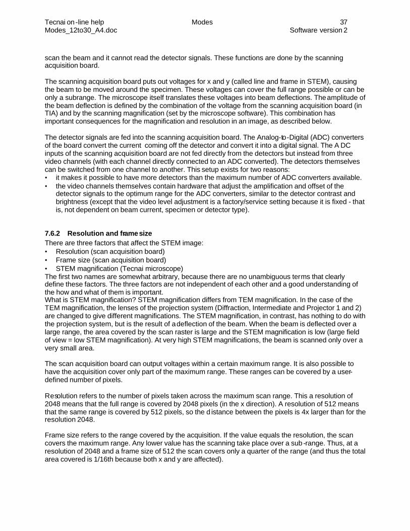
Tecnai on -line help Modes 37 Modes_12to30_A4.doc Software version 2
scan the beam and it cannot read the detector signals. These functions are done by the scanning acquisition board. The scanning acquisition board puts out voltages for x and y (called line and frame in STEM), causing the beam to be moved around the specimen. These voltages can cover the full range possible or can be only a subrange. The microscope itself translates these voltages into beam deflections. The amplitude of the beam deflection is defined by the combination of the voltage from the scanning acquisition board (in TIA) and by the scanning magnification (set by the microscope software). This combination has important consequences for the magnification and resolution in an image, as described below. The detector signals are fed into the scanning acquisition board. The Analog-to-Digital (ADC) converters of the board convert the current coming off the detector and convert it into a digital signal. The A DC inputs of the scanning acquisition board are not fed directly from the detectors but instead from three video channels (with each channel directly connected to an ADC converted). The detectors themselves can be switched from one channel to another. This setup exists for two reasons: • it makes it possible to have more detectors than the maximum number of ADC converters available. • the video channels themselves contain hardware that adjust the amplification and offset of the
detector signals to the optimum range for the ADC converters, similar to the detector contrast and brightness (except that the video level adjustment is a factory/service setting because it is fixed - that is, not dependent on beam current, specimen or detector type).
7.6.2 Resolution and frame size There are three factors that affect the STEM image: • Resolution (scan acquisition board) • Frame size (scan acquisition board) • STEM magnification (Tecnai microscope) The first two names are somewhat arbitrary, because there are no unambiguous terms that clearly define these factors. The three factors are not independent of each other and a good understanding of the how and what of them is important. What is STEM magnification? STEM magnification differs from TEM magnification. In the case of the TEM magnification, the lenses of the projection system (Diffraction, Intermediate and Projector 1 and 2) are changed to give different magnifications. The STEM magnification, in contrast, has nothing to do with the projection system, but is the result of a deflection of the beam. When the beam is deflected over a large range, the area covered by the scan raster is large and the STEM magnification is low (large field of view = low STEM magnification). At very high STEM magnifications, the beam is scanned only over a very small area. The scan acquisition board can output voltages within a certain maximum range. It is also possible to have the acquisition cover only part of the maximum range. These ranges can be covered by a user-defined number of pixels. Resolution refers to the number of pixels taken across the maximum scan range. This a resolution of 2048 means that the full range is covered by 2048 pixels (in the x direction). A resolution of 512 means that the same range is covered by 512 pixels, so the d istance between the pixels is 4x larger than for the resolution 2048. Frame size refers to the range covered by the acquisition. If the value equals the resolution, the scan covers the maximum range. Any lower value has the scanning take place over a sub -range. Thus, at a resolution of 2048 and a frame size of 512 the scan covers only a quarter of the range (and thus the total area covered is 1/16th because both x and y are affected).
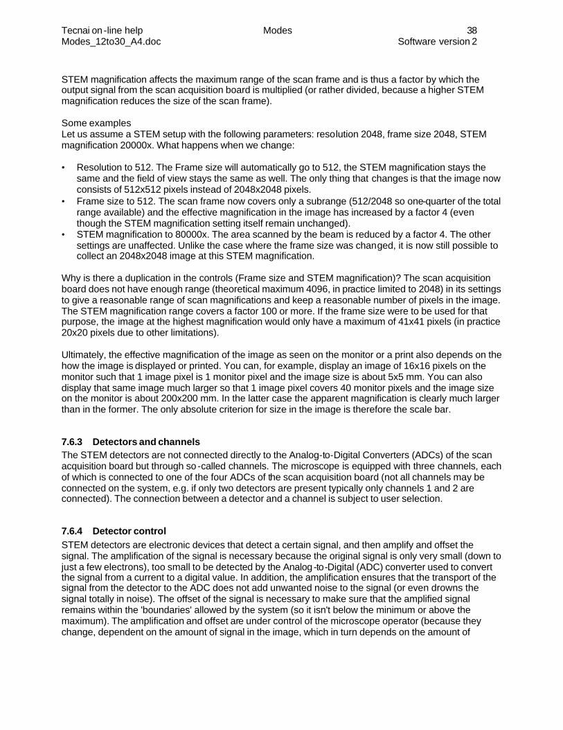
Tecnai on -line help Modes 38 Modes_12to30_A4.doc Software version 2
STEM magnification affects the maximum range of the scan frame and is thus a factor by which the output signal from the scan acquisition board is multiplied (or rather divided, because a higher STEM magnification reduces the size of the scan frame). Some examples Let us assume a STEM setup with the following parameters: resolution 2048, frame size 2048, STEM magnification 20000x. What happens when we change: • Resolution to 512. The Frame size will automatically go to 512, the STEM magnification stays the
same and the field of view stays the same as well. The only thing that changes is that the image now consists of 512x512 pixels instead of 2048x2048 pixels.
• Frame size to 512. The scan frame now covers only a subrange (512/2048 so one-quarter of the total range available) and the effective magnification in the image has increased by a factor 4 (even though the STEM magnification setting itself remain unchanged).
• STEM magnification to 80000x. The area scanned by the beam is reduced by a factor 4. The other settings are unaffected. Unlike the case where the frame size was changed, it is now still possible to collect an 2048x2048 image at this STEM magnification.
Why is there a duplication in the controls (Frame size and STEM magnification)? The scan acquisition board does not have enough range (theoretical maximum 4096, in practice limited to 2048) in its settings to give a reasonable range of scan magnifications and keep a reasonable number of pixels in the image. The STEM magnification range covers a factor 100 or more. If the frame size were to be used for that purpose, the image at the highest magnification would only have a maximum of 41x41 pixels (in practice 20x20 pixels due to other limitations). Ultimately, the effective magnification of the image as seen on the monitor or a print also depends on the how the image is displayed or printed. You can, for example, display an image of 16x16 pixels on the monitor such that 1 image pixel is 1 monitor pixel and the image size is about 5x5 mm. You can also display that same image much larger so that 1 image pixel covers 40 monitor pixels and the image size on the monitor is about 200x200 mm. In the latter case the apparent magnification is clearly much larger than in the former. The only absolute criterion for size in the image is therefore the scale bar.
7.6.3 Detectors and channels The STEM detectors are not connected directly to the Analog-to-Digital Converters (ADCs) of the scan acquisition board but through so -called channels. The microscope is equipped with three channels, each of which is connected to one of the four ADCs of the scan acquisition board (not all channels may be connected on the system, e.g. if only two detectors are present typically only channels 1 and 2 are connected). The connection between a detector and a channel is subject to user selection.
7.6.4 Detector control STEM detectors are electronic devices that detect a certain signal, and then amplify and offset the signal. The amplification of the signal is necessary because the original signal is only very small (down to just a few electrons), too small to be detected by the Analog-to-Digital (ADC) converter used to convert the signal from a current to a digital value. In addition, the amplification ensures that the transport of the signal from the detector to the ADC does not add unwanted noise to the signal (or even drowns the signal totally in noise). The offset of the signal is necessary to make sure that the amplified signal remains within the 'boundaries' allowed by the system (so it isn't below the minimum or above the maximum). The amplification and offset are under control of the microscope operator (because they change, dependent on the amount of signal in the image, which in turn depends on the amount of
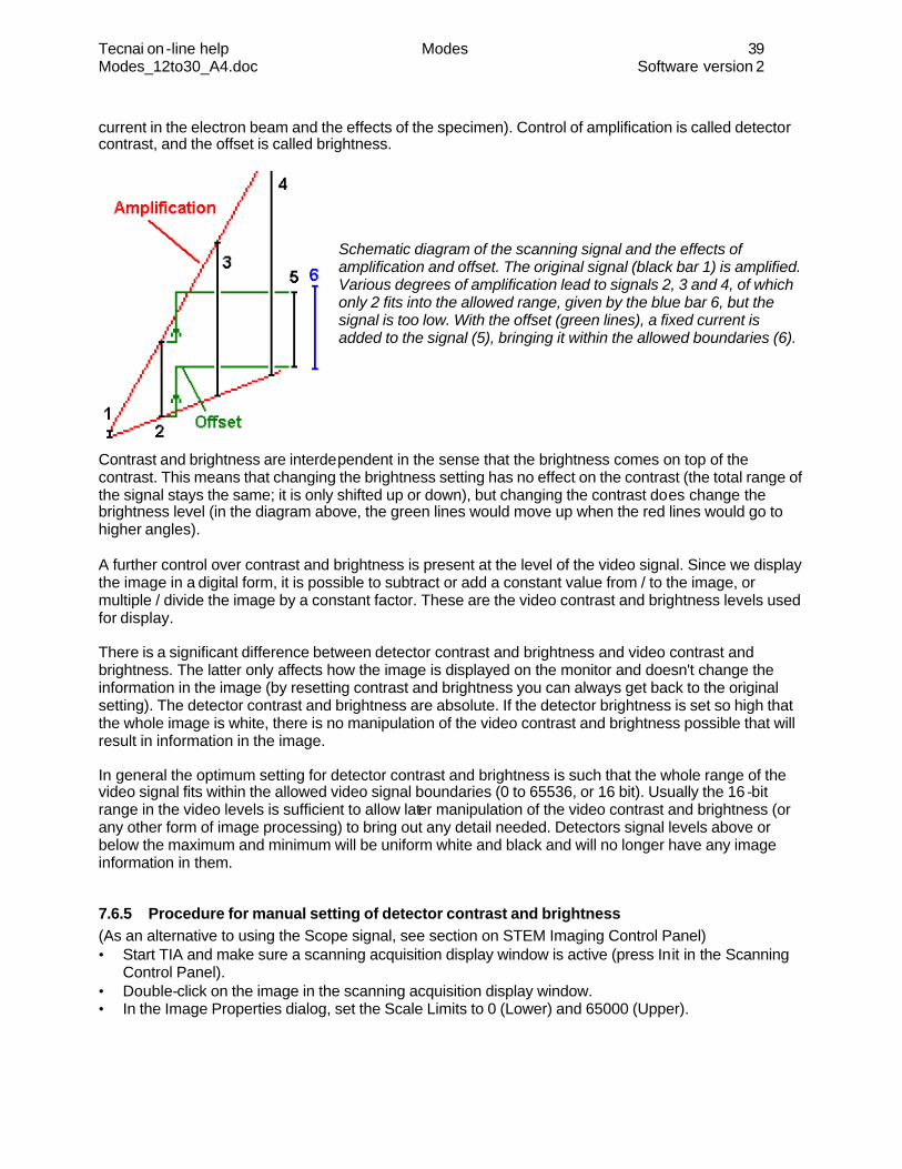
Tecnai on -line help Modes 39 Modes_12to30_A4.doc Software version 2
current in the electron beam and the effects of the specimen). Control of amplification is called detector contrast, and the offset is called brightness.
Schematic diagram of the scanning signal and the effects of amplification and offset. The original signal (black bar 1) is amplified. Various degrees of amplification lead to signals 2, 3 and 4, of which only 2 fits into the allowed range, given by the blue bar 6, but the signal is too low. With the offset (green lines), a fixed current is added to the signal (5), bringing it within the allowed boundaries (6).
Contrast and brightness are interdependent in the sense that the brightness comes on top of the contrast. This means that changing the brightness setting has no effect on the contrast (the total range of the signal stays the same; it is only shifted up or down), but changing the contrast does change the brightness level (in the diagram above, the green lines would move up when the red lines would go to higher angles). A further control over contrast and brightness is present at the level of the video signal. Since we display the image in a digital form, it is possible to subtract or add a constant value from / to the image, or multiple / divide the image by a constant factor. These are the video contrast and brightness levels used for display. There is a significant difference between detector contrast and brightness and video contrast and brightness. The latter only affects how the image is displayed on the monitor and doesn't change the information in the image (by resetting contrast and brightness you can always get back to the original setting). The detector contrast and brightness are absolute. If the detector brightness is set so high that the whole image is white, there is no manipulation of the video contrast and brightness possible that will result in information in the image. In general the optimum setting for detector contrast and brightness is such that the whole range of the video signal fits within the allowed video signal boundaries (0 to 65536, or 16 bit). Usually the 16 -bit range in the video levels is sufficient to allow later manipulation of the video contrast and brightness (or any other form of image processing) to bring out any detail needed. Detectors signal levels above or below the maximum and minimum will be uniform white and black and will no longer have any image information in them.
7.6.5 Procedure for manual setting of detector contrast and brightness (As an alternative to using the Scope signal, see section on STEM Imaging Control Panel) • Start TIA and make sure a scanning acquisition display window is active (press Init in the Scanning
Control Panel). • Double-click on the image in the scanning acquisition display window. • In the Image Properties dialog, set the Scale Limits to 0 (Lower) and 65000 (Upper).
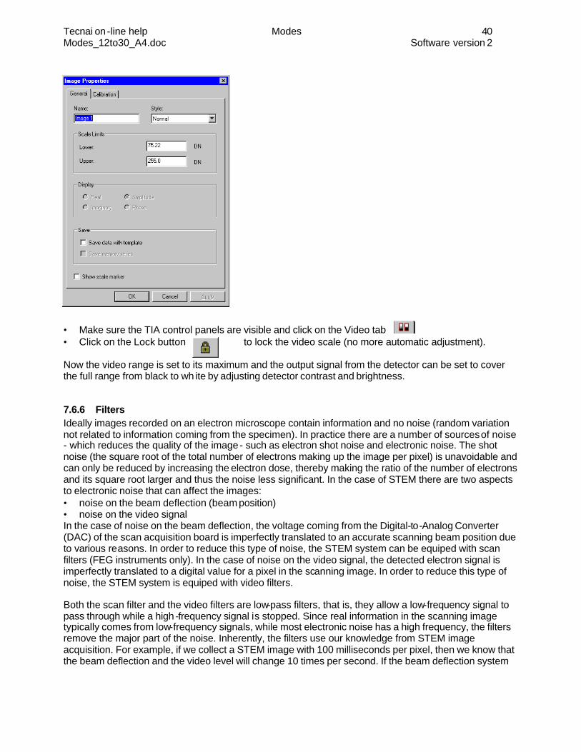
Tecnai on -line help Modes 40 Modes_12to30_A4.doc Software version 2
• Make sure the TIA control panels are visible and click on the Video tab • Click on the Lock button to lock the video scale (no more automatic adjustment). Now the video range is set to its maximum and the output signal from the detector can be set to cover the full range from black to wh ite by adjusting detector contrast and brightness.
7.6.6 Filters Ideally images recorded on an electron microscope contain information and no noise (random variation not related to information coming from the specimen). In practice there are a number of sources of noise - which reduces the quality of the image - such as electron shot noise and electronic noise. The shot noise (the square root of the total number of electrons making up the image per pixel) is unavoidable and can only be reduced by increasing the electron dose, thereby making the ratio of the number of electrons and its square root larger and thus the noise less significant. In the case of STEM there are two aspects to electronic noise that can affect the images: • noise on the beam deflection (beam position) • noise on the video signal In the case of noise on the beam deflection, the voltage coming from the Digital-to-Analog Converter (DAC) of the scan acquisition board is imperfectly translated to an accurate scanning beam position due to various reasons. In order to reduce this type of noise, the STEM system can be equiped with scan filters (FEG instruments only). In the case of noise on the video signal, the detected electron signal is imperfectly translated to a digital value for a pixel in the scanning image. In order to reduce this type of noise, the STEM system is equiped with video filters. Both the scan filter and the video filters are low-pass filters, that is, they allow a low-frequency signal to pass through while a high -frequency signal is stopped. Since real information in the scanning image typically comes from low-frequency signals, while most electronic noise has a high frequency, the filters remove the major part of the noise. Inherently, the filters use our knowledge from STEM image acquisition. For example, if we collect a STEM image with 100 milliseconds per pixel, then we know that the beam deflection and the video level will change 10 times per second. If the beam deflection system

Tecnai on -line help Modes 41 Modes_12to30_A4.doc Software version 2
or video signal changes much more rapidly than that, it must be due to noise. We can then smooth out the rapid variation (noise) to end up with a better STEM image. The scan filter is needed only on FEG systems . It is set in the STEM Imaging Scan (Expert) control panel. For this beam deflection filter there are four settings, Off (very fast scanning), Fast, Medium and Slow (slow scan image acquisition). When the scan filter is in automatic mode, it will be adjusted to the scanning speed. In manual control, which is only available by experts, the use of the wrong setting can lead to excessive noise (Off while doing the final image acquisition slowly) or image distortion especially at the left-hand side where each new line starts (Slow while scanning very rapidly). The filter must therefore be matched to the scan speed used. Only experts can override the automatic mode. The v ideo filter is set in the STEM Detector Selection (Expert) control panel. For the video filter, each channel has a wide range of settings, selectable from a drop-down list. The filters can also be controlled automatically in which case they are matched to the scan speed. In manual control, which is only available to experts, the correct filter setting can be determined by lowering the value until the image starts to have horizontal streaks (signal variations are smeared out over several pixels). Now increase the value again by approximately two steps (or at least until the streaks are completely absent).

Tecnai on -line help Modes 42 Modes_12to30_A4.doc Software version 2
8 EFTEM EFTEM (Energy-Filtered TEM) makes use of the fact that (some of) the beam e lectrons lose energy inside the specimen (this process is called inelastic scattering). Energy losses on the one hand degrade the image (since electrons that have lost energy are focused differently from those that have not lost any energy, strong energy losses result in image blurring, an effect that increases in strength with specimen thickness). On the other hand, the energy losses contain specific information about the specimen (chemical and physical). In EFTEM, the electrons are separated according to their energies, making it possible to filter out the blurring effects or retrieve the chemical or physical information from the specimen.
8.1 General introduction to energy filtering When passing through a specimen, electrons interact with it. Some are scatte red without losing energy (elastic scattering, e.g. in the case of crystals Bragg scattering) which implies that the electrons are deflected by a certain scattering angle and no longer form part of the transmitted beam. Other electrons lose energy inside the specimen by interacting for example with electrons in the specimen itself. Often this takes the form of a beam electron ejecting an electron from its orbit around the nucleus of an atom in the specimen. The beam electron loses an amount of energy (at the very least the amount needed to eject the specimen electron) and the atom loses an electron and often reacts by emitting an X ray. Energy losses are always accompanied by scattering through an angle as well. The inelastic scattering angles are generally much smaller than elastic scattering angles and, in contrast with Bragg scattering, are variable. Statistically, the inelastic scattering angles increase with the energy loss. The average scattering angles for low energy losses is low and these electrons effectively remain part of the transmitted beam (they cannot be stopped by the objective aperture). For higher energy losses the larger angles makes it possible to stop these electrons with the objective aperture. When the energy-loss electrons are separated according to their energy, they form an energy-loss spectrum. A typical energy-loss spectrum consists of the zero-loss peak (those electrons that have lost no or negligible energy), and towards higher energy losses a signal that at first increases strongly (within the first 50 volts, usually with a maximum around 25 volts) and then decays towards high energy. The decay is not monotonous but superimposed on this general background are so-called energy loss edges (regions where the signal first rises steeply, then decays again towards higher energy), which are the result of energy losses through interactions with specific atoms (the edges are thus element-specific). The amount of inelastic scattering increases with specimen thickness (in general quite rapidly), dependent on the incident electron energy and on the material the beam is interacting with (in general the heavier the material, the stronger the interaction). An important parameter for EFTEM is the so-called Mean Free Path, which is a dimension tha t indicates the pathlength inside the specimen wherein all electrons (statistically speaking) will have undergone one inelastic scattering event (since some electrons will have undergone multiple scattering by then, after one mean free path there still remain some unscattered electrons). Typical mean free paths are of the order of 50-100nm for 120kV electrons, 100-200 for 200kV and 150 -300 for 300kV. Above one mean free path is is still possible (and often even advantageous) to filter images in order to remove energy-loss electrons. However, the other main application - elemental mapping - becomes much more difficult and often even impossible at such specimen thicknesses. For good elemental mapping ultra -thin specimens are therefore important.
8.2 The (post-column) Imaging Filter For EFTEM, the microscope is equipped with an Imaging Filter, which is mounted underneath the projection chamber (a so -called post-column filter, as opposed to an in-column filter, where the filter itself forms part of the microscope column). The Filter accepts electrons passing through an entrance aperture
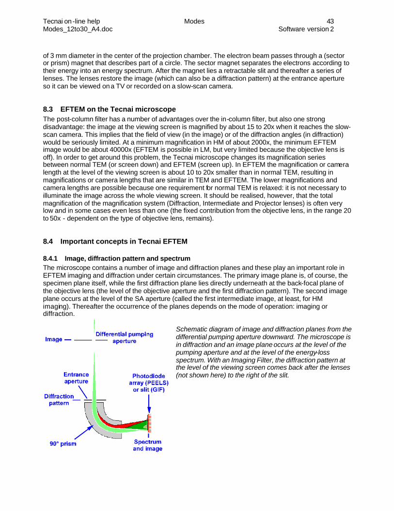
Tecnai on -line help Modes 43 Modes_12to30_A4.doc Software version 2
of 3 mm diameter in the center of the projection chamber. The electron beam passes through a (sector or prism) magnet that describes part of a circle. The sector magnet separates the electrons according to their energy into an energy spectrum. After the magnet lies a retractable slit and thereafter a series of lenses. The lenses restore the image (which can also be a diffraction pattern) at the entrance aperture so it can be viewed on a TV or recorded on a slow-scan camera.
8.3 EFTEM on the Tecnai microscope The post-column filter has a number of advantages over the in-column filter, but also one strong disadvantage: the image at the viewing screen is magnified by about 15 to 20x when it reaches the slow-scan camera. This implies that the field of view (in the image) or of the diffraction angles (in diffraction) would be seriously limited. At a minimum magnification in HM of about 2000x, the minimum EFTEM image would be about 40000x (EFTEM is possible in LM, but very limited because the objective lens is off). In order to get around this problem, the Tecnai microscope changes its magnification series between normal TEM (or screen down) and EFTEM (screen up). In EFTEM the magnification or camera length at the level of the viewing screen is about 10 to 20x smaller than in normal TEM, resulting in magnifications or camera lengths that are similar in TEM and EFTEM. The lower magnifications and camera lengths are possible because one requirement for normal TEM is relaxed: it is not necessary to illuminate the image across the whole viewing screen. It should be realised, however, that the total magnification of the magnification system (Diffraction, Intermediate and Projector lenses) is often very low and in some cases even less than one (the fixed contribution from the objective lens, in the range 20 to 50x - dependent on the type of objective lens, remains).
8.4 Important concepts in Tecnai EFTEM
8.4.1 Image, diffraction pattern and spectrum The microscope contains a number of image and diffraction planes and these play an important role in EFTEM imaging and diffraction under certain circumstances. The primary image plane is, of course, the specimen plane itself, while the first diffraction plane lies directly underneath at the back-focal plane of the objective lens (the level of the objective aperture and the first diffraction pattern). The second image plane occurs at the level of the SA aperture (called the first intermediate image, at least, for HM imaging). Thereafter the occurrence of the planes depends on the mode of operation: imaging or diffraction.
Schematic diagram of image and diffraction planes from the differential pumping aperture downward. The microscope is in diffraction and an image plane occurs at the level of the pumping aperture and at the level of the energy-loss spectrum. With an Imaging Filter, the diffraction pattern at the level of the viewing screen comes back after the lenses (not shown here) to the right of the slit.
Tecnai on -line help Modes 44 Modes_12to30_A4.doc Software version 2
In image mode, one image plane lies at the level of the viewing screen (or plate camera), with a second one at the level of the recording camera of the Imaging Filter (behind the imaging lenses of the Filter itself). In this mode, a diffraction plane occurs at the level of the differential pumping aperture (a 200 mm aperture that separates the projection chamber from the column) and a second at the slit of the Filter. The second diffraction plane thus combines a diffraction pattern with a spectrum. In diffraction mode, all image and diffraction planes are reversed with respect to the image mode. One important aspect about these image and diffraction planes is the inverse relation between magnification or camera length of these planes. Thus, if the magnification in image mode is high, then the size (camera length) of the diffraction pattern in the differential pumping aperture and at the slit of the Filter is small. If the image magnification is low, then the diffraction patterns are large. And, since the magnification series for EFTEM contain extremely small real magnification, the diffraction patterns in the pumping aperture and at the Filter slit can be enormous! The same applies to the images when the microscope is in diffraction with a small camera length. Under these circumstances (low magnifications, small camera lengths) alignments become highly critical and some phenomena may appear: • Astigmatism that can be strong and increases to lower magnifications due to charging of the slit of
the Filter. If the diffraction pattern at the spectrum plane becomes very large, the slit not only cuts off energy-loss electrons but also works like a very small and asymmetric objective aperture. This may lead to increasing image astigmatism towards lower magnifications. To avoid or reduce such effects, use a small objective aperture (thereby removing most of the diffracted beams) and use a somewhat larger slit width.
• The slit becomes visible as a shadow in the image or diffraction pattern. At low magnifications or camera lengths the electrons beams go through high angles relative to each other and, due to spherical aberration, cannot be focused properly at a single plane - the slit - causing the higher-angle beams to be cut off. Increase the size of the slit, if possible.
• Slight beam shifts make the diffraction pattern disappear at low camera lengths. When the image at the differential pumping aperture becomes very large (as happens at low camera lengths), even slight beam shifts may cause the beam to be intercepted by the differential pumping aperture. Use the specimen stage rather than the beam shift for aligning the area of interest for diffraction.
8.4.2 Cross-over correction From the discussion above, it will be clear that for proper EFTEM operation at low magnifications or small camera lengths the alignment of the beam in the differential pumping aperture will be critical (otherwise the whole beam may be blocked and no image or diffraction pattern is obtained at all). For this purpose a so -called cross-over alignment is used (the beam goes through a cross-over in the differential pumping aperture). The cross-over alignment shifts the image or diffraction pattern in the differential pumping aperture. When the microscope is aligned properly, the image or diffraction pattern on the screen does not shift. There is one important aspect to the cross-over correction: in image mode the cross-over correction is the same as a diffraction shift and vice versa (the cross-over correction uses the same image deflection coils as the image/diffraction shift. This means for example that the alignment values of the diffraction shift (the centering of all diffraction pattern together, not the alignment of the individual camera lengths) also affect the cross-over correction. Also if (by accident) a diffraction shift is executed in image mode (such as happens when the Diffr shift is constantly active on the Multifunction knobs), the cross-over correction will be affected.
8.4.3 Normalizations The image or diffraction shifts used for the image/diffraction alignment and the cross-over alignment can be very sensitive to the actual values of the magnetic fields of the lenses in the projection system

Tecnai on -line help Modes 45 Modes_12to30_A4.doc Software version 2
(Diffraction, Intermediate and Projector lenses). The lens normalizations bring these lenses to more reproducible settings - and, as a consequence, more reproducible image/diffraction shifts and cross-over corrections. It is therefore advised to allow the microscope to execute a projector-system normalization whenever the magnification or camera length is changed (an alternative to the automatic normalization it is also possible to do the normalization by hand, by assigning projector normalization to one of the Control Pad user buttons).
8.4.4 SA diffraction Because of the cross-over correction (which shifts the image while in diffraction, but the shift occurs before the SA aperture so the 'area of interest' moves relative to the SA aperture), SA diffraction is difficult to execute in EFTEM. In addition, the larger area of selection (relative to CBED) causes problems at low camera lengths (because the image in the differential pumping aperture and spectrum planes is so large) such as diffraction astigmatism that cannot be corrected. The best procedure for SA diffraction in EFTEM is as follows: • Focus the beam on (an uninteresting area of) the specimen. Use no SA aperture. • Switch to EFTEM and select a suitable camera length. Set up everything as needed. • Go back to normal TEM image operation. • Defocus the beam somewhat (but still no SA aperture) and center the area of interest in the beam. • Go again to EFTEM diffraction and observe the shadow image in the central (transmitted beam). • Insert an SA aperture (it should be visible from the shadow it casts in the diffraction shadow image). • Center the SA aperture around the area of interest. • Defocus the beam further until the beams in the diffraction pattern shrink to spots.