Technology Transfer and Early Industrial Development:Evidence from the Sino-Soviet Alliance

Michela Giorcelli Bo Li∗

January 30, 2022

This paper studies the causal effect of technology and knowledge transfers on early indus-trial development. Between 1950 and 1957, the Soviet Union supported the “156 Projects”in China for building technologically advanced industrial facilities. We exploit idiosyncraticdelays in project completion and the unexpected end of the Sino-Soviet Alliance, and showthat receiving both Soviet technology and know-how had large, persistent effects on plantperformance, while the effects of receiving only Soviet capital goods were short-lived. Theintervention generated horizontal and vertical spillovers, and production reallocation fromstate-owned to privately owned companies since the late 1990s.

aKeywords: Industrialization, Technology Transfer, Knowledge Diffusion, ChinaJEL Classification: L2, M2, N34, N64, O32, O33

a

∗Contact information: Michela Giorcelli, University of California, Los Angeles, and NBER, 9262 BuncheHall, 315 Portola Plaza, Los Angeles CA, 90095, USA. Email: mgiorcelli@econ.ucla.edu; Bo Li: TsinghuaUniversity PBC School of Finance, Email: lib@pbcsf.tsinghua.edu.cn. Boxiao Zhang provided excellentresearch assistance. We thank David Atkin, Bruno Caprettini, Dora Costa, Michele Di Maio (discus-sant), Alvaro Garcia, Rick Hornbeck (discussant), Jiandong Ju, Naomi Lamoreaux, Nicholas Li, ErnestLiu, Kalina Manova (discussant), Nathan Nunn, Luigi Pascali, Nancy Qian, Xuan Tian, John Van Reneen,Eric Verhoogen, Guo Xu, Ting Xu (discussant), and Elira Kuka, Jared Rubin, and Danila Serra throughthe Adopt-a-Paper program. We also thank seminar and conference participants at Harvard, UCLA, YaleUniversity, Berkeley Haas, University of British Columbia, University of Michigan, George Washington Uni-versity, Auburn University, Wilfrid Lauriel University, University of Oxford, LUISS, Universitá di Bologna,Universitá di Padova, University of Melbourne, Tsinghua University, the NBER Summer Institute on on Pro-ductivity, Development and Entrepreneurship, the Cliometrics Conference, the NBER Productivity Lunch,the Second Women in International Economics (WIE) Conference, the AFA, the CEPR/LEAP Workshopin Development Economics, the Barcelona GSE Summer Forum on the Economics of Science and Innova-tion, the Pacific Conference for Development Economics, the Webinar Series in Finance and Development(WEFIDEV), the LSE Asia Economic History Seminar, the Online Economic History Workshop, and theRidge Conference for helpful comments and discussion. We are also thankful to senior officials at Statis-tics China for declassifying the historical data for this research and to historians at the National ArchivesAdministration of China for their help in accessing archival materials.

1 Introduction

International technology and knowledge flows are key drivers of economic development. Nu-merous works have shown that the adoption of foreign technologies may lead to a substantialboost in firm productivity in less-advanced economies (Pavcnik, 2002; Goldberg et al., 2009;Bloom et al., 2013; Hardy and Jamie, 2020). Consequently, technology transfer interven-tions have been widely used to promote industrialization in developing countries (Hoekmanet al., 2004; Robinson, 2009), especially through the diffusion of state-of-the-art capitalgoods (Stokey, 2020). However, in their early stages of industrialization, countries lack notonly modern capital goods but also industry-specific knowledge that allows pioneering firmsto succeed (Mostafa and Klepper, 2018). Acquiring this knowledge is complex: several ofits elements are “tacit” or embodied in workers and organizations and are often obtainedthrough extensive on-the-job training from foreign companies (Chandra, 2006).

Despite the importance of technology and knowledge transfer programs, little is knownabout which interventions work in fostering firm and industry growth in the first phases ofa country industrialization. Moreover, which program components help firms move fromadopting foreign technology to developing their own in not very well understood. Theempirical research has been held back mostly by lack of long-term firm-level data and naturalvariation in the delivery of such interventions. Moreover, it is challenging to disentangle theeffects of technology embedded in foreign capital goods from those of know-how diffusionand human capital training, as they often occur simultaneously.

This paper studies the causal effect of technology and knowledge transfers on early in-dustrial development, using evidence from the Sino-Soviet Alliance. In the 1950s, to helpthe industrialization of the newly formed People’s Republic of China, the Soviet Unionsupported the development of the so-called 156 Projects, an array of technologically ad-vanced, large-scale, capital-intensive industrial facilities.1 Based on the initial agreements,the projects were supposed to receive a “basic” technology transfer that involved the dupli-cation of whole Soviet plants through the provision of Soviet state-of-the-art machinery andequipment; and an “advanced” know-how and knowledge transfer via visits of Soviet expertsto teach Chinese high-skilled technicians how to operate the new machineries, and to offertechnical and industrial management training to the engineers and production supervisors.The Soviet transfer was considered a vital factor in Chinese development. Its investments,which accounted for 45% of Chinese GDP in 1949, allowed China to receive the best So-viet technology, which in the steel and iron industries was considered the best in the world(Lardy, 1995; Gangchalianke, 2002; Zhikai and Wu, 2002).1 We say “so-called” because 156 projects were originally contemplated and because the identifying labelhas persisted to this day in China. However, only 139 projects involving Soviet technology transfer wereeventually signed and approved between 1950 and 1957.

2

We use newly assembled data on the 156 Projects signed between 1950 and 1957, matchedwith declassified data on their plant performance yearly until 2000 for the steel industry andwith firm-level data in 1985 and between 1998 and 2013 for all the industries.

Our identification strategy relies on idiosyncratic delays in project completion due to Sovietconstraints in providing capital goods and experts to train their Chinese counterparts. Whenthe Sino-Soviet Split in 1960 ended the alliance between the two countries, all the plantsbelonging to the 156 Projects had already been built, but only part of them had receivedthe Soviet transfers. Specifically, some plants had received both Soviet machinery andequipment and technical assistance (advanced plants), some others had only gotten Sovietmachinery and equipment (basic plants), while the remaining ones didn’t get any Sovietmachinery or technical assistance and ended up employing traditional domestic technology(comparison plants). Notably, basic, advanced and comparison plants had very similarobservable characteristics, were located in comparable geographical areas, and operated inthe same industries. Moreover, their outcomes were on the same trends in the five yearsbefore receiving the Soviet intervention.

We find three key results. First, using plant-level data for the steel industry from 1949 to2000, we show that receiving a basic transfer had positive but short-lived effects on plantperformance, while the impact of the advanced transfer was large and persistent. Output ofbasic plants differentially increased relative to that of comparison plants up to six years afterreceiving Soviet machineries, reaching a 14.7 percent peak. After that, the effects startedslowly decreasing and were no longer significant after 20 years, the estimated like cycle ofSoviet capital. By contrast, output of advanced plants rose by 19.7 percent within 20 years,relative to that of basic plants, reaching a cumulative effect of 49.5 percent after 40 years.Advanced plants also produced better-quality steel and were systematically more productive,while employing similar inputs to basic and comparison plants. Second, declassified firm-level data in 1985 and between 1998 and 2013 in all industries confirm the short-lived impactof the basic transfer and the long-lasting effect of the advanced transfer.

Third, we investigate why only the impact of the advanced transfer persisted over years.We show that, in the 1960s and 1970s, when China’s interaction with foreign countries wasextremely limited, only advanced plants were able to develop new production processes andhome-fabricate modern machineries and equipment, which ultimately replaced Soviet capitalwhen it became obsolete. Moreover, once China began gradually opening to internationaltrade since 1978, advanced plants relied dramatically less on the import of foreign capital,and they systematically engaged more in trade due to producing better-quality output thanbasic and comparison plants. By contrast, we do not find evidence that our results aredriven by special ex-post government favors to advanced or basic plants, by better politicalconnections, or by selection on unobservable plant characteristics.

3

The major goal of the Soviet technology transfer was to create large industrial facilities topush local industrial development. Was the program successful in doing so? We documentthat the existence of positive spillovers was largely related to the presence of advanced plants.Both plants in the same firms of advanced plants and plants in other firms horizontally andvertically related to them increased their production and their productivity, relative tosimilar plants related to basic plants, adopted the same technology of the advanced plantswhen China was a closed economy, and followed their export patterns when China openedup to international trade. Conversely, these variables did not differentially change betweenplants related to basic and comparison plants.

Starting in the late 1990s, the Chinese government undertook a number of market lib-eralization reforms. We therefore test if the spillover effects persisted after this majorinstitutional change. We find that, between 1998 and 2013, firms that became privatelyowned and were economically related to advanced plants had better performance and weremore productive. At the county-level, these changes were associated to an increased shareof industrial output produced by private firms. The main driver of these results seem to bethe fact that counties that hosted advanced plants had a higher concentration of industry-specific human capital. In fact, advanced plants offered training programs for engineersand created professional schools for high-skilled technicians that were institutionalized overyears (Hirata, 2018). In the long run, counties that hosted advanced plants were more likelyto offer STEM degrees and had higher number of technical schools relative to counties thathosted basic plants, that may have helped firms to hire better educated workers when theystarted competing for inputs in the local labor market.

Finally, we assess the contribution of the Soviet transfer to the Chinese aggregate growthrate between 1950 and 2008. An additional basic project increased province-level outputon average by 1.1 percent per year, and an additional advanced project by 6.2 percent. Aback-of-the-envelope calculation shows that, without the basic and the advanced transfer,Chinese real GDP per capita growth between 1953 and 1978 would have been between 7and 19 percent lower, confirming their vital importance in Chinese industrialization.

The contribution of this paper is threefold. First, our paper relates to the growing lit-erature examining the effects of industrial policies and technology transfer on structuraltransformations. Several works have shown the importance of investments in heavy indus-tries to foster early stage economic development and their positive long-run consequences(Mitrunen, 2019; Choi and Levchenko, 2021; Kim et al., 2021; Lane, 2021). Our work con-tributes to this strand by comparing large industrial facilities that use foreign-importedtechnologies to similar plants that rely on domestic capital goods, and by disentanglingthe effects of technology transfers embodied in physical capital goods relative to the tacithuman capital component that accompanies such transfers. Our context is China, which

4

experienced the “the fastest sustained expansion by a major economy in history” (Morrison,2019). Moreover, by showing that knowledge diffusion and on-the-job training are essentialfor ensuring persistent effects of industrial policies, our paper also related to the literaturethat studies the role of foreign firms in seeding industry-specific know-how that can sub-sequently push the growth of a developing country’s industry (Mostafa and Klepper, 2018;Keller and Yeaple, 2013; Yeaple, 2013).

Second, we contribute to the literature that studies the role of technology diffusion indeveloping countries (see Verhoogen, 2020 for a comprehensive review). Previous papershave documented the positive impact of technology adoption on short-run performance ofsmall and medium-sized firms (Pavcnik, 2002; Mel et al., 2008; Goldberg et al., 2010; Bloomet al., 2013; Bruhn et al., 2018; Hardy and Jamie, 2020) and the existence of substantialbarriers to its adoption (Atkin et al., 2017; Bloom et al., 2020; Juhász et al., 2020). To thebest of our knowledge, this paper is the first to use nonexperimental data to examine theeffects of international technology and knowledge transfer on the largest industrial facilitiesof a country, following them from their foundation to recent times.

Third, this work is related to the large literature on spillover effects. Existing researchhas focused on spillovers determined by foreign direct investments and the opening of largenew plants (Javorcik, 2004; Javorcik et al., 2008; Greenstone et al., 2010; Alfaro-Urena etal., 2019), worker mobility (Stoyanov and Zubanov, 2012), managerial knowledge diffusion(Bloom et al., 2020; Bianchi and Giorcelli, 2022), and sectoral industrial policies (Liu, 2019;Fan and Zou, 2021; Lane, 2021). Our setting allows us to disentangle the spillover effectsof technology transfer from knowledge spillovers that follow know-how diffusion, and theirinteractions with major institutional changes. In terms of context, a closely related paperis Heblich et al. (2020) that also studies the Sino-Soviet technology transfer. However,they focus on long-run negative spillovers of the 156 Projects on counties that hosted them,relative to counties suitable to host them that were eventually not selected. By contrast,our paper looks at differences within the 156 Projects, using plant-level data and assessingshort, medium and long-run direct effects and spillover effects.

The rest of this paper is organized as follows. Section 2 describes the Sino-Soviet Alliance.Section 3 describes the data. Section 4 discusses the empirical framework and the identifica-tion strategy. Section 5 studies the effects of the technology transfer on firm-level outcomes.Sections 6 and 7 examine the spillover and aggregate effects. Section 8 concludes.

5

2 The Sino-Soviet Alliance and Technology Transfer

2.1 The Birth of the Sino-Soviet Alliance

With the end of WWII, a bipolar international order emerged, dominated by the confronta-tion and competition between the United States and the Soviet Union. For both powers,a strategic alliance with China was crucially important (Lardy, 1995). Since 1927, Chinahad been intermittently enmeshed in a civil war fought between the Kuomintang-led gov-ernment of the Republic of China (ROC) and the Communist Party of China. The U.S.government supported the Kuomintang and the government of the ROC by providing mil-itary, economic, and political assistance,2 but in 1949, the Communist Party emerged asvictorious. China’s war came to an end, and the People’s Republic of China (PRC) wasformed. Despite some initial Soviet distrust, the PRC’s inspired principles and economicsystem provided the ideological basis for cooperation with the Soviet Union. On February14, 1950, the two countries signed the “Sino-Soviet Treaty of Friendship, Alliance, and Mu-tual Assistance,” which marked the start of large-scale economic and military cooperationand the Soviet Union’s official recognition of the PRC as a strategic partner (Zhang et al.,2006). In response to the Sino-Soviet Alliance, the United States and its allies imposedeconomic sanctions against the PRC in the 1950s and stopped all trade activities with thecountry until 1978.

2.2 The Soviet Technology Transfer Setup

At the end of China’s civil war, the country’s economy was largely premodern. Almosttwo-thirds of output was agricultural, less than one-fifth industrial, and the few industrialfactories built during the Japanese occupation had been destroyed during WWII bombing(Lardy, 1995, p. 144). The newly formed government adopted a centralized, planned-economy model, based on state ownership of all economic activities and large collectiveunits in agriculture (Perkins, 2014). Market forces were largely eliminated, and industrialinputs and outputs were allocated according to quotas established by subsequent Five-YearPlans. Wages were set by the government, which allocated workers to jobs.

The First Five-Year Plan (1953–1957) declared that one of the new government’s majorgoals was to build a modern industrial system. However, the country lacked technicalknowledge and expertise to do so on its own. Several Chinese leaders admitted that, “[...]at the beginning [they] didn’t quite understand what should be done first and what should2 On December 16, 1945, U.S. President Truman described the policy of the United States with respect toChina as follows: “It is the firm belief of this government that a strong, united, and democratic China isof the utmost importance to the success of the United Nations Organization and for world peace” (UnitedStates of America Government Printing Office, 1945, p. 945).

6

be done later in industrial development, and how to coordinate various departments givenlimited inputs” (Ji, 2019). Therefore, PRC officials pressed hard for technology transfer fromthe Soviet Union (Zhang et al., 2006, p. 110). Between 1950 and 1957, the two countriessigned various agreements for the construction of the 156 Projects. These projects focusedon heavy industries, such as metallurgy, machinery, electricity, coal, petroleum, and chemicalraw materials—the Chinese government was intending to mimic the development model ofthe Soviet Union in the 1930s. The total value of such investments amounted to $80 billion(in 2020 figures; $20.2 billion in 1955 RMB), equivalent to 45.7% of Chinese GDP in 1949and 144.3% of its industrial output.

Through this program China received the most advanced technology available in the SovietUnion, which in industries like iron and steel was the best in the world (Gangchalianke, 2002).For instance, during the 1950s the Soviet Union built and operated the world’s best blastfurnaces—these were installed in Chinese plants in Anshan, Wuhan, and Paotou before evenbeing employed in Soviet factories (Lardy, 1995; Zhikai and Wu, 2002).3 The advancementof Soviet technology was recognized from the US side as well. After studying the Soviet andChinese industries for decades, Clark (1995) argued that Soviet steel technology transferredto China was comparable to that of the most developed Western economies. The Soviet effortin promoting Chinese management of the 156 Projects impressed the Indian Prime MinisterNehru. While visiting the Anshan plant, he compared the Soviet transfer in China with theBritish and US one in India, concluding that in China “the entire process of production in theenterprise [was] being operated by Chinese experts,” while in India the British and Americans“never allow[ed] Indians to manage the most important mechanism of the enterprises” (Zhikaiand Wu, 2002; Hirata, 2018).

The locations for the 156 Projects were chosen based on geological conditions and accessto natural resources. For example, experts from the Soviet Ministry of Metallurgy explainedthat the nonferrous metal plants, such as the Guizhou Aluminum Company, “must be builton copper rich ore,” and that “the copper content of the ore should be tested during thesite selection.” Beyond the geological conditions, Chinese leaders had a strong preferencefor choosing inner regions and mountain areas to protect these plants from potential mil-itary attacks (Lardy, 1995). For these reasons, the 156 Projects were concentrated in thenortheastern regions (Heilongjiang, Jilin, Liaoning) and the inner regions (Shaanxi, Shanxi,Gansu, and Hubei, Figure 1). Only 10 projects were built on sites where firms existed before1949. These firms were almost completely destroyed during the Civil War and were no longer3 The Soviet Union did not provide any aid in the form of grants; it lent China only $2.9 billion ($300 millionin 1955 dollars ) in response to a Chinese request for 10 times that amount. This loan shall be used to“repay the Soviet Union’s delivery of machinery and equipment [...]. China shall trade raw materials, tea,agricultural products at foreign exchange rates to repay principal and interest from December 31, 1954,to December 31, 1963” (Lardy, 1995). The prices of machinery, equipment, raw materials, and othercommodities were calculated according to world market prices.

7

able to produce; therefore, they were rebuilt from scratch (Hirata, 2018). In this respect,the Soviet assistance shaped the geographical distribution of Chinese industrialization, sincebefore 1952 the few existing firms were almost all located in the coastal areas (Lardy, 1995).

Chinese leaders, and in particular Chairman Mao Zedong, initially envisioned two typesof transfers for all the 156 Projects: a “basic” technology transfer and an “advanced” know-how and knowledge transfer. More specifically, the “basic” technology transfer involved theduplication of whole Soviet plants, the provision of Soviet state-of-the-art machinery andequipment, as well as help in surveying geological conditions, selecting plant sites, directingplant construction, and supplying blueprints. The “advanced” know-how and knowledgetransfer involved visits of Soviet experts to teach Chinese high-skilled technicians how tooperate the new machineries, and to offer within-firm technical and industrial managementtraining to the engineers and production supervisors. The engineer training included classesin math, physics, and chemistry, as well as lectures in organizational, technological, andplanning methods. The supervisor training, based on “scientific management” principles,included operational-planning classes, instructions on assigning workers to the most ap-propriate tasks, and the introduction of quality-control methods (Clark, 1973).4 The Sovietexperts were expected to spend on average three years in Chinese plants, sharing engineeringdesigns, product designs, and other technical data (Zhang et al., 2006).5

However, the Soviet leaders cautioned the Chinese counterpart they could not commit tosuch a massive technology and knowledge transfer due to lack of resources. Nevertheless,they offered to provide technical assistance based on experts availability and to share 4,000product designs to improve technological innovations, increase equipment operation ratesand product quality, and decrease both production costs and the amount of raw materialsused (Zhang et al., 2006; Hirata, 2018; Ji, 2019).

2.3 Delays in the 156 Projects, and the Sino-Soviet Split

Despite the promises of Soviet Union and the rosy picture of “Great Friendship” promulgatedby the authorities, the 156 Projects suffered serious difficulties and experienced many moredelays than initially predicted both by the Soviet and the Chinese sides. On the ground,machinery, equipment, and designs ordered from the Soviet Union almost always arrived orstarted operating later than planned, due to constraints on Soviet production capacity, lackof Soviet experts able to visit Chinese plants, and miscommunication between Soviet and4 Starting in the early 1930s, Soviet planners under Stalin selectively adopted the latest American manage-ment methods; they invited many Western companies, including the Ford Motor Company to invest inthe Soviet Union (Hirata, 2018).

5 Despite numerous references to Soviet technical personnel in the Chinese press, no reliable totals areavailable on the number of Soviet military and civilian specialists assigned to Communist China. Accordingto the statistics recorded by the Soviet Ministry of Foreign Affairs, 5,092 Soviet technical personnel wereworking in China between 1952 and 1959.

8

Chinese experts (Filatov, 1975; Hirata, 2018). The Soviet Union did not have machinery andequipment in reserve, and by 1955 almost every Soviet industrial area had received ordersfor capital goods from China that proved difficult to deliver (Zhang et al., 2006). Between1955 and 1960, one-third of annual Soviet production of steel-rolling equipment was forChina. Further complicating matters, the Sino-Soviet Alliance descended into turmoil inthe late 1950s over political and ideological disputes. Despite attempting to maintain abilateral relationship in the early 1960s, the two countries couldn’t reach an agreement, andthe formal end of their cooperation in 1963 became known as the Sino-Soviet Split. Longbefore that, the 156 Projects had already been dramatically reduced in scope and number.In 1960, the Soviet Union suddenly withdrew its experts from China and stopped providingmachinery and equipment.

These practical and political matters strongly affected the completion of the 156 Projects.For instance, the Benxi Iron and Steel Company, built to replicate the Red October (KrasnyOktyabr) factory in Volvograd, was expected to receive Soviet machinery and equipment in1955, but never got them. As this material was about to be shipped, a fire destroyed criticalequipment in the Red October factory, which then blocked the shipment to Benxi. SovietUnion ensured that it would produce it later, after its plant operations could resume, butdue to the Split this never happened (Filatov, 1975).

The lack sufficient numbers of experts to help oversee plant construction and installationof new machinery and equipment was also a major deal. For example, Soviet experts whowere supposed to visit the Fushun Aluminum Plant in 1959 never did so—they were retainedto deal with an unexpected breakdown in the Volkhov Aluminum Plant and by the timethey finished this task the Split had occurred. As a consequence, Fushun eventually receivedSoviet machinery, but without any training despite what was initially planned between thetwo countries (Filatov, 1980).

Similarly, the language barriers between Soviet and Chinese teams required the constantpresence of translators, but this, too, proved problematic. Soviet experts expected to visitthe Changchun First Automotive Plant in 1955 had to wait until their translators learnedChinese, which prevented the Chinese plant from starting its operations on schedule (Borisovand Koloskov, 1980). Long-distance bilingual communication fostered additional problems.When Soviet experts arrived at the Jilin Daheishan Molybdenum Mine Plant, they realizedtheir designs did not fit, as the initial written communication was misunderstood and lettersrequesting additional clarifications went lost (Kiselev, 1960). The attempts of providing thenew designs failed due to the upcoming Split.

In light of these delays even before the Split, it would have been profitable for China toprioritize the most promising projects, but the country faced many challenges in doing so.In fact, each project was unique, aimed at replicating a specific Soviet plant, which made

9

it impossible to reallocate machinery or equipment across the 156 Projects (Filatov, 1975).And unfortunately, the Soviet experts who did arrive in China were proficient only in the useof specific machinery and their translators had been trained in project-specific terminology,which limited their employment to the projects they were initially allocated to (Borisov andKoloskov, 1980).

Consequently, the Chinese government decided to start plant operations with domesticcapital goods and replace them with Soviet machineries as soon as they were delivered. Forthis reason, in 1960, when the Split occurred, all the plants belonging to the 156 Projectswere already been built and were producing. However, they largely differed for the technolo-gies in use. In fact, some plants had received both Soviet machinery and equipment thatreplaced domestic capital and technical assistance, and some others had only gotten Sovietmachinery and equipment. The remaining ones didn’t get any Soviet machinery or techni-cal assistance and continued producing with domestic capital (Clark, 1973). The country’slimited access to the foreign technology market after 1950 forced it to rely solely on its ownresources until at least 1978.

In the rest of the paper we will refer to projects and plants that got both Soviet machineryand equipment and technical assistance as advanced projects or advanced plants ; to projectsand plants that got only Soviet machinery and equipment as basic projects or basic plants ;and to projects and plants that didn’t get any Soviet machinery or technical assistance ascomparison projects or comparison plants.

3 Data

We collected and digitized different types of historical and administrative data from primarysources. In this section, we document our data-collection process and describe the datacollected. Additional details and definitions of the variables appear in Appendix B.

3.1 The 156 Projects

We started our data collection by compiling a list of the 156 Projects envisioned under theSino-Soviet Alliance, from the official agreements between the Soviet Union and the PRCstored at the National Archives Administration of China. As previously mentioned, whileinitial discussions between Chinese and Soviet leaders aimed at 156 Projects, the numberof civil projects signed and approved between 1950 and 1957 was 139. For each project,we collected detailed information on its name and location, the name of the plant built,industry, size and capacity.

Of the 139 approved projects, 46 were basic projects, 47 were advanced projects and

10

46 were comparison projects (Table 1, columns 5-7). Most projects were located in China’snortheastern and interior regions, for strategic reasons and for proximity to natural resources,and only 10 (7.1%) were built on the site of plants existing before 1949 and destroyed duringthe Civil War (Figure 1). The projects called for the construction of large industrial plants;each employing on average 39,910 workers, for a total of around 5.5 million workers—a mere3 percent of China’s total workforce, but almost 40 percent of the country’s employmentin the industrial sector in 1952. The projects were overwhelmingly concentrated in heavyindustries. The electricity sector accounted for 23.0% projects, the machinery sector for21.6%, the coal sector for 20.1%, and the steel and nonferrous metal industries for 14.4%and 10.1%, respectively (Figure A.1). Only two projects (1.4%) were in light industry. Theaverage planned investment amounted to $580.3.4 million, and the projects’ mean durationwas expected to be 5.6 years (Table 1, column 1).

3.2 Plant- and Firm-Level Data

We manually collected and digitized restricted, plant-level annual reports compiled yearly bythe Steel Association for the 94 steel firms operating in China from 1949 to 2000, for a totalof 1,410 plants. The reports contain rich information on plant performance, such as quantityand type of steel products, utilization of inputs, capacity, the specific machinery in use, andnumber and types of workers (unskilled workers, high-skilled workers, and engineers). Usingplant name, location, county, and province, we manually and uniquely matched the 304steel plants across 20 firms belonging to the 156 Projects with their outcomes from the SteelAssociation reports. 91 plants received a basic transfer, 98 an advanced transfer and 115did not get any Soviet transfer (Table 2, columns 1-3).

A natural question is whether plant performance data that represent the core of our anal-ysis are accurate. For instance, plant supervisors may have had incentives to misreportsome data to meet the goals set by the central government or to show better-than-actualperformance. To attenuate this concern, we assert three points. First, the Steel Associa-tion reports were highly monitored and checked by industry peers, which strongly limitedthe possibility of manipulation. Moreover, the officially-released aggregate production datawas complied by Statistics China, a different and independent source. Manipulations weretherefore more likely to occur in the latter rather than in the former reports. Second, afterthe Sino-Soviet Split, the Chinese government wanted to tie up loose ends with the SovietUnion as quickly as possible.6 Therefore, if any manipulation occurred, it should have aimedat underestimating rather than overestimating the impact of the Soviet technology transfer,6 For instance, China rushed to repay Soviet immediately, even though it could have done so over ten years(Zhang et al., 2006).

11

especially in the long run. This would go against us finding results.7 Third, we cross-checkour data with several sources. In particular, we rely on the studies of the US ProfessorGardner Clark, who examined the Chinese steel industry between 1949 and 1993, by visit-ing over multiple trips Chinese steel plants with the goal of assessing the quality of capitalthey were using (Clark, 1995). His works conclude that the data from the Steel AssociationReports, our main source, appear credible.8 More details about our data cross-check can befound in Appendix B.

We also manually collected and digitized confidential, firm-level data from the SecondIndustrial Survey, conducted by Statistics China in 1985 and declassified for this project.This survey is the first and the most comprehensive dataset on Chinese industrial enterprisesbetween 1949 and the early 1990s. It covers more than 40 industries within the industrialsector, containing firm-level data for the 7,592 largest firms operating in China in 1985.The survey gathered data on each firm’s output, sales, profits, fixed assets, raw materials,total wages, number of employees, finished product inventory, main products, productionequipment, and year of establishment. Using name, location, and province, we manuallyand uniquely matched all 139 firms that were part of the 156 Projects to their performancein 1985. From the Survey, we also collected and digitized county-level and prefecture-levelindustrial production data.9

Finally, we manually matched all 139 firms in the 156 Projects with their 1998–2013performance from the China Industrial Enterprises database. This database, compiled yearlyfrom 1998 to 2013, covers more than 1 million public and private industrial enterprises abovea designated size in China.10 It includes a rich set of information on firms: firm output,number of employees, and profits, as well as ownership structure and capital investment.

3.3 Statistical Yearbooks

We manually collected and digitized province-level data on GDP, population, capital, in-vestment, and number of workers from the Statistical Yearbooks compiled yearly between1949 and 2000 by Statistics China. These data confirm that the PRC was little industrial-ized in 1950. The average share per province of firms in the agricultural sector was 85%,accounting for 80% of total provincial output. By contrast, the share of provincial output in7 For instance, during the Great Leap Forward, the Chinese government wanted to show the efficacy oflabor-intensive methods of industrialization, which would emphasize manpower rather than machines andcapital expenditure, in stark contrast with the goals of the Soviet transfer (Clark, 1973; Lardy, 1995).

8 More specifically, in Table B.1, we repeat our main analysis using Clark (1995)’s data, which lead toresults fully consistent with our main findings.

9 Counties are Chinese administrative areas, comparable to U.S. counties. Provinces are Chinese adminis-trative areas, comparable to U.S. states. Prefecture cities are Chinese administrative areas, larger thancounties but smaller than states.

10 The data include firms whose asset value exceeds 5 million yuan prior to 2011, and 20 million yuan after2011.

12

heavy industries was less than 18%. Between 1952 and 1985, Chinese economy experiencedstructural transformation: heavy industries uniformly increased their shares of production,at the expense of light industries (Figure A.2, Panel A).

As China adopted a planned-economy model, government control over industry dramati-cally increased. In 1952, 48.7% of the firms were privately owned, while state-owned corpo-rations comprised only 20.2%. By 1965, more than 90% of firms were state-owned (FigureA.3, Panel A). During the same period, the agriculture industry was commonly organizedinto state-controlled cooperatives. Also, the location of industrial activities gradually shiftedfrom the coastal regions to the country’s interior (Figure A.3, Panel B)—consistent with thefact that most of the 156 Projects were located in the interior regions for strategic reasonsand for proximity to natural resources.

4 Identification Strategy

The identification strategy of this paper relies on the delays in completion of the 156 Projectsthat arose after their start. When in 1960 the Soviet Union suddenly interrupted the tech-nology transfer program, some plants had received both Soviet machinery and equipmentand technical assistance (advanced plants), some others had only gotten Soviet machineryand equipment (basic plants), while the remaining ones didn’t get any Soviet machinery ortechnical assistance and ended up employing traditional domestic capital goods (comparisonplants).

We estimate the effects of the Soviet technology transfer via the following equation on the304 steel plants belonging to the 156 Projects:

outcomeit = ↵i + �t +40X

⌧=�5

�t(Basici · Years after Transfer=⌧ it) (1)

+40X

⌧=�5

�t(Advancedi · Years after Transfer=⌧ it) + ✏it

outcomeit is logged output and TFP11 of plant i at time t ; Basici is an indicator for plants thatreceived a basic transfer; Advancedi is an indicator for plants that received an advanced transferon top of a basic transfer; Years after Transfer=⌧it is an indicator when a calendar year is ⌧ yearsbefore or after the year in which plant i received the Soviet transfer. Since equation 1 is an eventstudy, we need to impute values for Years after Transfer=⌧it for comparison plants. To this end, weassume that they would have been treated in 1960, the year of the Spilt. However, our results arerobust to alternative imputations, as explained in Section 5.1. The excluded year is ⌧ = �1. Plant11 Specifically, we compute either TFPQ or TFPR based on the possibility of measuring firm physical output

or only revenues. Details about their estimation can be found in Appendix C.

13

fixed effects ↵i control for variation in output over plants that is constant over time. Calendaryear fixed effects �t control for variation in output over time that is common across all plants.Standard errors are clustered at the plant level. As all plants were still alive and state-owned in2013, equation 1 estimates an intensive margin effect.

Under the identification assumption that the transfer eventually received (or not received) by aplant was orthogonal to its characteristics or its potential success, the coefficient �t captures theeffect of receiving a basic transfer on plant performance, relative to plants that did not receive anySoviet transfer ⌧ years after its implementation; the coefficient �t captures the additional effect ofreceiving an advanced transfer on top of a basic transfer ⌧ years after its implementation. Theremainder of this section provides evidence in support of the research strategy.

4.1 Were Basic, Advanced and Comparison Projects Comparable

at the Time of Approval?

We test whether basic, advanced and comparison projects were comparable when they were signedand approved. To do so, we perform an ANOVA test for mean equality on several baseline projectcharacteristics between the three groups. First, we compare the approval and start year of projects.In fact, projects that eventually received a basic or an advanced transfer may have been approvedor started earlier than the comparison ones and so more likely to have been finished before theSplit. However, we do not find significant differences among the three groups (Table 1, columns5–8). Second, we check if comparison projects were more complex and therefore harder to completebefore the Spit than the basic or the advanced ones. The ANOVA test fails to reject the hypothesisof mean equality between the three groups of projects in terms of planned and actual investment, theplanned and actual number of workers, the value of equipment supposed to be received from SovietUnion, the expected project length, and the expected capacity. Similarly, the share of projectsbuilt on the site of firms destroyed during the Sino-Japanese war is substantially the same betweenbasic, advanced and comparison projects. Finally, we test whether basic or advanced projects mayhave located in more accessible areas than the comparison projects. The difference in distance fromnational and provincial borders, the coast and Treated Ports where most economic activities wereconcentrated, and railroads and roads is not statistically different among them.

Despite the similarity in their observable characteristics, basic or advanced projects may havebeen concentrated in areas or sectors with an ex-ante higher potential to grow relative to thecomparison projects. To rule out this hypothesis, we estimate the predicted probabilities (marginaleffects) from a multinomial logit model, where the dependent variable – that takes different valuesfor basic, advanced and comparison (baseline) projects – is regressed on a full set of province orindustry fixed effects. None of the estimated coefficients is statistically significant (Figure 2, PanelsA and B). This indicates that projects in specific provinces or industries did not have a higherprobability of receiving a basic or an advanced transfer, relative to the baseline of not receiving any

14

Soviet transfer.12 Moreover, we test if counties in which basic, advanced and comparison projectswere located were similar before the Soviet intervention. OLS regressions predicting county-levelnumber of firms, population, employment share and government funding in 1953 do not showstatistically significant differences among counties hosting the three groups of projects (Table A.1,columns 1-4).

Taken together, these results are fully consistent with the historical records that explain howproject delays were caused by constraints on Soviet production capacity, limited supply of Sovietexperts and translators, and miscommunication between the two countries’ experts, but were notrelated to project-specific characteristics (Filatov, 1975; Hirata, 2018).

4.2 Were Basic, Advanced and Comparison Plants Comparable be-

fore Receiving the Soviet Transfers?

We next check if basic, advanced and comparison plants were comparable the year before receivingthe Soviet transfer, by regressing plant characteristics and outcomes on indicators for receiving abasic and an advanced transfer and a fully set of firm fixed effects. None of the twenty-six estimatedcoefficients, all small in magnitude, is statistically significant (Table 2, columns 4-5). We concludethat the three groups of plants were statistically equivalent before receiving the Soviet transfer.

4.3 Were Basic, Advanced and Comparison Plants Comparable on

the Same Trend before Receiving the Soviet Transfers?

We test whether basic, advanced and comparison plants were on the same trend in the five yearsbefore receiving the Soviet transfer. We first estimate a constant linear time trend model in whichwe interact a constant linear trend with indicators for receiving a basic and an advanced transfer.The estimated coefficients are close to zero and not statistically significant (Table A.2). Moreover,the estimated coefficients on the indicators alone are not statistically different from zero in all thespecifications, confirming the results of the balancing tests of Table 2.

Second, we replace the linear time trend with a full set of indicators for each year before receivingthe Soviet transfer and interaction of each indicator with indicators for receiving a basic and anadvanced transfer. The estimated coefficients on the indication terms are small in magnitude andnever statistically significant from zero (Table A.3). Moreover, some are positive and some arenegative, confirming lack of any pattern. Finally, the F -statistics at the bottom of each panelindicate that we can never reject the null hypothesis that the interaction terms are jointly equal tozero.

These findings suggest that basic, advanced and comparison plants were following a similar trendin the five years before receiving the Soviet transfer.12 Repeating this analysis at the prefecture city and county level leads to the same findings (Figure A.4,

Panels A and B).

15

4.4 Were Resources Reallocated across Basic, Advanced and Com-

parison Plants?

A potential threat to our identification strategy arises if the Chinese government reallocated theSoviet machinery or workers from basic and advanced to comparison projects before or after theSplit. First, it is worth noting that this scenario would go against us finding results. Second,since each project was aimed at replicating specific Soviet plants, China could not reallocate theSoviet machinery, equipment, experts, or translators to the most promising projects before the Split(Filatov, 1975). After the Split, the records on capital owned by plants indicate that basic andadvanced plants did indeed retain the Soviet equipment. It would have been unprofitable for thegovernment to temporarily shut down treated plants and replace brand-new machines, especiallyin light of the difficulties the country was facing in manufacturing capital goods on its own (Zeitz,2011; Ji, 2019). Regarding the workforce, individual records to trace worker movement do notexist, to the best of our knowledge, but the historical records indicate that engineers in basic andadvanced plants were employed to train other engineers, but only from nearby factories (Zhang etal., 2006; Hirata, 2018). Moreover, migration in China at that time was highly restricted thanks tothe household registration (hukou) system, which made worker movements from basic and advancedto comparison plants extremely rare.

5 Effects of Technology Transfer on Firm Performance

In this section, we study the effect of the Soviet technology transfer on firm outcomes. For the steelindustry, we have a plant-level panel dataset from 1949 to 2000. For the other industries, we usefirm-level data in 1985 and between 1998 and 2013.

5.1 Plant-Level Results in the Steel Industry

The results of estimating equation 1 on plants in the steel industry indicate that receiving a basictransfer had positive but short-lived effects on plant performance, while the impact of the advancedtransfer was large and persistent.

Output of basic plants was not significantly larger than that of comparison plants for the firsttwo years after receiving Soviet machineries. It then started differentially growing, reaching a 14.7percent higher level six years after the Soviet intervention. After that, the effects started slowlydecreasing and were no longer significant after 20 years (Figure 3, Panel A). By contrast, output ofadvanced plants rose by 8.4 percent relative to that of basic plants within two years since the Soviettransfer and by 19.7 percent within 20 years. The gap between the two groups of plants continuedto increase up to 40 years after the program, reaching a cumulative effect of 49.5 percent (Figure3, Panel B). These findings are largely driven by the increased performance of basic and advancedplants, while output of comparison plants remained mostly flat during this time period (Figure 3,Panel C).

16

Soviet technology transfer also affected the quality of steel. Relative to comparison plants thatwere using domestic blast furnaces, the introduction of open-hearth furnaces in basic plants in-creased the production of crude steel (considered the best-quality steel) and reduced the quantitiesof pig iron (considered of lower quality given its higher carbon content) up to 10 years.13 When thelife-cycle of Soviet machineries estimated to be 15 years at the time ended, basic plants stoppedproducing higher-quality steel (Table A.4, columns 1–2). Conversely, the increase of crude steel andreduction in pig iron production in advanced plants remained systematically higher than in basicplants (Table A.4, columns 1–2). This outcome was likely due to the adoption of better produc-tion methods, that became embedded in firm organizations (Zhang et al., 2006). For instance, theadoption of Soviet methods of analysis that systematically sampled hot metals reduced the timeto determine their chemical composition from 50 minutes to 2 minutes. This allowed necessaryadjustments to be made more quickly, and led in turn to higher output quantity and quality in theshort and in the long run (Clark, 1973).

We next investigate the effects of Soviet transfer on productivity. Specifically, we estimate totalfactor productivity quantity as logTFPQ=logTFPR-log ep, where ep is the revenue-share weightedaverage of the prices of plant products and total factor productivity revenue (TFPR) is calculatedusing Gandhi et al. (2020)’s method. The dynamic of productivity follows a similar pattern asoutput. Specifically, TFPQ of basic plants rose up to six years after Soviet transfer with a 14.5percent increase relative to comparison plants, and was no longer significant after 20 years. Con-versely, TFPQ of advanced plants increased between 8.3 percent two years after the Soviet transferto 47.9% after 40 years, relative to basic plants (Figure 3, Panel B).

We further explore the increase in productivity by focusing on the different components of theproduction function. The increase in TFPQ appears to be driven largely by output growth, sinceinputs, such as number of worker and coke and iron quantities, were not statistically differentbetween basic, advanced and comparison plants (Table A.4, columns 3–5). This also indicatesthat the government did not allocate more inputs to basic or advanced plants and therefore theirincreased performance is due to the Soviet transfer and not some other differential treatments.

A potential concern in interpreting the productivity results is that the Chinese economy was anoncompetitive environment until at least the late 1980s: all plants in a given industry faced thesame prices in a given year. However, any non-market clearing prices set by the government wouldbe absorbed by year fixed effects. Moreover, we do not have any bias due to unobservable plant-specific variation in output or input prices. Finally, as the steel sector is regarded as strategic bymost governments, even in non-planned economies its production is subject to widespread indus-trial policy interventions, whose goals “do not necessarily coincide with value creation and profitmaximization” (Mattera and Dilva, 2018).14

13 Specifically, open-hearth furnaces facilitate the control of carbon content, by allowing period samplingand interim analysis of the heat, which is not possible with blast furnaces.

14 It is worth noting that we can estimate a gross-output production function rather than a value-addedproduction function. As explained in Gandhi et al. (2017), the percentage increase in value-added will belarger than in gross output, given the value of intermediate inputs that are not differentially changing inour context.

17

Another issue may be that Chinese government-set prices may not be reliable indicators of under-lying input quality, which may generate the so-called “quality bias.” For instance, basic or advancedplants may have used the same quantity of better-quality inputs as comparison plants. We test forthe possibility of quality bias as follows. First, we aggregate output and inputs using their averageannual prices as reported by the American Iron and Steel Institute, and we compute TFPR andTFPQ with these values. The estimates using Chinese and U.S. prices are very similar in magnitude(Table C.2, column 2). Consistent with these results, the historical records indicate that Chineseprices indeed reflected quality differences. In 1985, for instance, Statistics China set the crudesteel price at 320RMB (US$199.22 in 2020 figures) per ton, compared to 249RMB (US$154.95 in2020 figures) per ton for pig iron. Second, following de Roux et al. (2020), who show that thetransmission bias and the quality bias offset when the production function is estimated with naiveOLS, we estimate TFPR and TFPQ with the OLS factor shares. The results are nearly identicalto those that use our baseline estimation (Table C.2, column 3).

Robustness Checks. Our findings are robust to a variety of modifications to the baselinespecification. Specifically, our results hold if we replace plant and year fixed effects with firm-yearfixed effects and county-year fixed effects (Table A.5, columns 2, 3, 6, and 7). While regressionswith plant and year fixed effects in the form of Equation 1 are widely used, a recent literaturedocuments possible shortcomings of these two-way fixed effects specifications (De Chaisemartinand D’Haultfoeuille, 2020; Goodman-Bacon, 2021; Borusyak et al., 2021). In particular, Sun andAbraham (2021) explains that, in presence of heterogeneous treatment effects, the coefficients onthe leads and lags of the treatment variable in an event study might place negative weights onthe average treatment effects for certain groups and periods. To address this concern, we use an“interaction-weighted” (IW) estimators, as proposed by Sun and Abraham (2021) themselves, whichis fully consistent with our baseline results (Table A.5, columns 4 and 8). We also impute values ofYears after Transfer=⌧ it to comparison plants using the values of the first year or the average yearin which basic and advanced plants received the Soviet transfer. The pattern and the magnitude ofour results remain substantially unchanged (Table A.6, columns 2, 3, 5, and 6). Next, we proposedifferent levels of standard-error clustering, that, in all cases, confirm the significance level of ourmain specification (Table A.7). Finally, to test for potential manipulation in our plant-level data,we use the estimates made by Clark (1995) that assessed the minimum and maximum possiblelevels of steel production, based on the capital in use in each steel plant. Even assuming that basicand advanced plants produced at the minimum and comparison plants at the maximum level, wewould still find a persistent effect of the advanced transfer and a short-lived effect of the basictransfer, in line with our main results (Table B.1, columns 4-8). As noted in Section 3.2, Clark(1995) conclude that the data from the Steel Association Reports are accurate.

5.2 Medium- and Long-Run Firm-Level Results in All Industries

For 1985 and between 1998 and 2013, the availability of large-scale data allows us to match all thebasic, advanced and comparison firms with their medium- and long-run economic outcomes. We

18

estimate the following equation:

outcomeit = ↵+ � · Basici + � · Advancedi + ✓cst + ⌫it (2)

where outcomeit is value added, TFPR calculated using Gandhi et al. (2020)’s method andworkers of firm i at time t ; Basici is an indicator for firms that received a basic transfer; Advancedi

is an indicator for firms that received an advanced transfer on top of a basic transfer; and ✓cst arecounty-sector-year fixed effects. Standard errors are clustered at the plant level. For estimation in1985, we don’t have a time dimension and we replace county-sector-year fixed effects with county-sector fixed effects.

These estimates confirm our main results from the steel industry. In 1985 and between 1998 and2013, value added, TFPR and employees of basic firms were not significantly different than those ofcomparison firms (Table A.8, columns 1, 3 and 5). By contrast, value added of advanced firms was,respectively, 41.5% and 52.0% higher than that of basic firms, and TFPR was 39.5% and 49.3%higher, with no differences in employment relative to basic plants (Table A.8, columns 2, 4 and 6).The magnitude of the estimates on the full sample are remarkably similar to those obtained fromthe steel-plant sample, which indicates that the Soviet technology transfer results apply beyond thesteel industry.

5.3 Mechanisms

Why did the effects of advanced transfer persist over time, while the effects of basic transfer wereshort-lived? In this section, we examine potential mechanisms. We start our analysis by lookingat production innovation and technology development. Between 1960 and until at least 1978, dueto the Soviet Split and the embargo of Western countries, Chinese firms could rely only on theirown resources to operate and innovate. During the 1960s, a new steel-making process, the basicoxygen, that blew oxygen through molten pig iron and lower the carbon content of the alloy, becamepredominant (Clark, 1973). According to the historical records, advanced plants were the only onesable to develop and adopt this process innovation (Ji, 2019). Data on production process in useby the steel plants indicate that, while basic plants were not more likely to use the basic oxygenprocess, advanced plants had a 25.2 percent higher probability of using it five years after the Soviettransfer and 65.1 percent higher probability twenty years after, relative to basic plants (Table 3,column 1). This finding is likely related to the organizational, technological, and planning classesadvanced plants received, whose goal was to improve factory operations and develop new and moreefficient production methods. It also explains why advanced plants produced more high-qualitycrude steel than basic plants and well beyond the life-cycle of the Soviet-imported machineries.

The Soviet capital was state-of-the-art in the 1950s and 1960s, but became obsolete in the 1970sand 1980s, due to the development of continuous casting furnaces (Fruehan et al., 1997). Data oncapital adoption indicate that only advanced plants home-fabricated the continuous casting furnacesthat were used to replace Soviet open-hearth ones. As a result, advanced plants were between 26.7

19

and 78.4 percent more likely to use this type of furnaces relative to basic plants between 10 to 20years after the Soviet transfer (Table 3, column 2). Conversely, basic plants did not show morecontinuous casting furnaces usage than comparison plants. This technological development mayexplain the long-lasting impact of the advanced transfer. While the effects of the basic transferfaded out twenty years after the Soviet intervention, when the estimated life-cycle of Soviet capitalended, advanced plants were able to replace it and continue striving.

In the late 1970s, China began gradually opening to international trade, especially with theWestern world. Among other effects, this implied that Chinese plants could import machines fromthe United States and Western Europe and export their products there. In light of the domesticdevelopment of new technologies, advanced plants relied dramatically less than basic plants on theimport of foreign capital. Nevertheless, they exported 45.5% more steel and produced 51.1% moresteel above the international standards than basic plants (Table 3, columns 3–5). This findingindicates that the quality of steel produced by advanced plants was recognized not only in China,but also by the international steel market. By contrast, we do not observe differential imports offoreign capital and exports between basic and comparison plants. This aspect can also contribute toexplain the short-lived effect of the basic transfer. When both types of plants could import foreignmachineries, basic plants did no longer have a productivity advantage over comparison plants.

We next examine whether the composition of plant human capital can be a mechanism for long-run persistence. The composition of human capital in the three types of plants was similar at timeof opening, as we have shown in our balancing tests (Table 2). However, over time, advanced plantsopened training schools for high-skilled technicians and offered within-firm training programs totheir engineers (Hirata, 2018; Ji, 2019). Consequently, advanced plants employed more engineersand high-skilled technicians and fewer low-skilled workers than basic plants, while the human capitalcomposition did not differentially change between basic treated and comparison plants (Table 4,columns 1–3). Better human capital likely boosted plant productivity, allowing the effects of theadvanced transfer to persist.

5.4 Alternative Explanations for the Technology Transfer Effects

Even if project delays represent a natural variation in the probability of receiving the Soviet transfer,it still may be the case that in subsequent years basic or advanced plants received special favors fromthe government that, in turn, allowed their performance to flourish. For instance, the governmentmay have allocated more funds to basic or advanced plants or may have invested more in countieswere these plants were located.

To investigate this potential issue, we first examine whether basic or advanced treated plantsreceived any special funding from the government. We find the government did not allocate moretransfers or granted more loans to basic or advanced plants relative to the comparison plants,neither in the short run nor in the long run (Table A.9, Panel A, columns 1–2).15 Moreover, we check

15 While we can observe yearly loans and transfers only for plants in the steel industry, looking at thesevariables in all 139 plants in 1985 and between 1998 and 2013 confirms the lack of differential and transfers

20

whether plants that received the Soviet transfer became more accessible to roads and railroads thancomparison plants after the intervention, which may have contributed to their success. However,we find that the distance from railroads and roads, statistically indistinguishable at the time of thetransfer, did not differentially change between the three groups of plants in the following decades(Table A.9, Panel A, columns 3–4).

Basic and advanced plants may have also become more politically connected than comparisonplants over time, or perhaps better politicians were allocated to their administrative areas. To testthis hypothesis, we collected data from the People’s Daily Online database, which includes names,city and year of birth, and education of both the secretaries of the Municipal Party Committee andthe mayors at the prefecture-city level from 1949 to 2018. The secretaries of the Municipal PartyCommittee were directly linked with the central government and were responsible for Party affairswithin the city area and for strengthening the Party’s leadership. In accordance with the instruc-tions of the higher-level Party committee, they carried out the work of Party agenda in the region,and they set up political and legal committees, the Party Committee’s organization department,and other departments. The mayors represented the local government and coordinated the work ofthe Municipal People’s Congress, the municipal government, and the provincial government. Wetherefore test whether secretaries and mayors that worked where basic or advanced plants werelocated were more likely to be born or have studied locally or whether they were more educatedthan those who worked where comparison plants were located. Having studied in the same ar-eas where where basic or advanced plants were located may reflect stronger links with local firmmanagement, while we use years of education as a proxy for politician quality. None of these fourmeasures is statistically different between basic, advanced and comparison plants in the 40 yearsafter the Soviet transfer (Table A.10, columns 1–6), which suggests that political connections andpolitician quality remained comparable over time.

Next, we check whether counties in which basic or advanced plants were located received moretransfers from the government than counties where comparison plants were located. We find thattotal investments, as well as investments in industries both related and unrelated to the 156 Projects,are not statistically different between the three groups of counties (Table A.11, columns 1–3).Similarly, the number of other industrial projects sponsored by the Chinese government after theSino-Soviet Split and the overall length of railroads and roads are substantially the same (TableA.11, columns 4–5).16 Taken together, these results do not support that the government favoredplants that received the Soviet transfer or the counties where they were located.

Since firm exit was virtually non-existent in China until the 1990s, one may wonder if the Chinesegovernment artificially kept alive comparison plants after the Sino-Soviet Split. This does not seemto be the case, as comparison plants, in spite of eventually not receiving any Soviet transfer,performed better and were larger than the other steel plants not included in the 156 Projects

between basic, advanced and comparison plants (Table A.9, Panel B).16 Other industrial projects sponsored by the Chinese government after the Split include the Construction

of the Third Front (TF), a massive yet short-lived industrialization campaign in China’s underdevelopedhinterland between 1964 and 1972. Fan and Zou (2021) document that the TF had long-run positiveaggregate effects on the local economy, regardless of the initial development level of the regions.

21

(Table A.12). While these results do not have any causal interpretation, they may indicate that,even if comparison plants were completed by the Chinese government alone, Soviet help in theirinitial planning was still beneficial.

In Section 4, we showed that basic and advanced plants exhibited similar observable character-istics relative to comparison plants. However, a potential concern to our identification may beselection on unobservable characteristics. To address this issue, we use the methodology proposedby Oster (2019), which assumes that the correlation between treatment and unobservables is equalto the correlation between treatment and observables multiplied by a factor �. A treatment effectis robust to selection on unobservables if it does not change sign at � = 1. This value of � meansthat the degree of selection on observed variables is the same as that on unobserved variables.17 InTable A.13, we show that our estimates change little relative to our main results as we move from� = 0.1 to � = 1 (columns 2–6). In order to have our treatment effects no longer significant, thedegree of selection on unobserved variables should be between 8 and 19 times larger than selectionon observed variables, values that are implausible (Table A.13, column 7). Therefore, our resultsdo not appear driven by selection on unobservables.

6 Spillover Effects

One goal of the Soviet technology transfer was to create large industrial facilities to push localindustrial development. In this section, we examine whether the transfer was successful in doingso, as well as the types of short-run and long-run spillovers it generated.

6.1 Spillovers across Plants within Firms

After absorbing the content of the Soviet training, advanced steel plants could have experiencedadditional improvements by transmitting new acquired knowledge to other plants in the same firm.To capture these effects, we estimate the following equation

outcomejft = ↵ft + �1 · Basicf + �1 · Advancedf + �2 · (Basicf · Postt)+

�2 · (Advancedf · Postt) + �3 · (Basicf · Postt · Post 1978t)+

�3 · (Advancedf · Postt · Post 1978t) + ⌘jft (3)

where outcomejft is one of the performance outcomes of of plant j in firm f at time t ; Basicf isan indicator for plants in the same firms of plants that received a basic transfer; Advancedf is anindicator for plants in the same firms of plants that received an advanced transfer on top of a basic17 Specifically, Oster (2019) shows that a treatment effect is robust if it does not change sign at � = 1

and Rmax = 1.3 · R̃, where Rmax is the R squared of a hypothetical regression of the outcome on bothobservables and unobservables. R̃ is the R squared of a regression of the outcome on just the observables.Table A.14 shows sensitivity to Rmax.

22

transfer; Post is an indicator for years after treated plants in firm f received the Soviet transfer;Post 1978 is an indicator for years after 1978, when China opened up to international trade; and↵ft are firm-year fixed effects. Standard errors are block-bootstrapped at the firm level with 1,000replications. We estimate equation 3 on the sample of plants not supposed to receive the Soviettransfer but already existing at the time of the Soviet intervention.o

The results support the existence of positive spillovers, mostly related to the advanced transfer.Before the Soviet transfer, we do not observe different performance among these plants: the coeffi-cients on the Basic and Advanced indicators are not statistically significant (Table 5, columns 1–5).After the Soviet intervention, while steel plants in the same firm of basic plants did not perform bet-ter than steel plants in the same firm of comparison plants, steel plants in the same firm of advancedplants increased their production of steel by 24.9 percent and were 22.1 percent more productive,relative to steel plants in the same firm of basic plants (Table 5, columns 1–2). These findings arelikely driven by the adoption of technologies developed by advanced plants. As indicated by thehistorical records (Lardy, 1995; Ji, 2019), advanced plants offered within-firm training programsthought which they shared their new technologies and better production methods. Consistently, wefind that plants in the same firm of advanced plants were more likely to use basic oxygen processand continuous-casting furnaces when China was a closed economy, and, when the country openedup to trade, these plants exported significantly more and produced a higher quantity of steel abovethe international standards (Table 5, columns 3–6).

6.2 Spillovers across Firms

We next examine whether the Soviet transfer generated spillover effects on other firms operatingeither in the same sector or in related sectors of the 156 Projects.

Horizontal Spillovers. We assess horizontal spillovers by estimating equation 3 on steel firms inthe same counties as basic, advanced and comparison plants, established before the Soviet transfersand by replacing firm-year fixed effects with county-year fixed effects. Steel plants in the samecounties of advanced plants, comparable before the Soviet transfer, showed better performancerelative to those in the same counties of basic plants after the intervention. Specifically, theyproduced 12.9% higher output and were 12.4% more productive (Table 6, columns 1–2), were morelikely to use basic oxygen converters and continuous-casting furnaces developed by advanced plants,and since 1978 they exported significantly more and produced a higher quantity of steel above theinternational standards. We do find evidence of positive horizontal spillovers from plants in thesame counties of basic plants relative to comparison plants.

Vertical Spillovers. The Soviet technology transfer may have generated spillovers on firmsin the supply chain of treated plants. To estimate these effects, first we identify steel-industryestablishemnts in the supply chain of basic, advanced and comparison plants by using the input-output matrix provided by the National Bureau of Statistics of China (NBS; see Appendix B.4).Second, we estimate equation 3 on steel plants located in the same counties of basic, advancedand comparison plants in nonsteel sectors, using county-year fixed effects instead of firm-year fixed

23

effects.Being a steel plant in the same county of a nonsteel basic plant is associated with higher produc-

tion relative to being in the same county of a nonsteel comparison plant. Compared to the latter,in the former the quantity of steel produced, comparable before the Soviet transfer, is 14.2 percenthigher (Table 7, column 1). These findings are fully consistent with the increased production ofbasic plants, which in turn may have affected their supply chain. However, only plants in the samecounty of advanced plants experienced a productivity increase after the Split, estimated to be 14.1percent, relative to plants in the same county of basic plants (Table 7, column 2). These companiesare also the only ones to register an increase in the probability of using basic oxygen convertersand continuous casting furnaces and that systematically engaged more in trade and produced moresteel above the international standards (Table 7, columns 3–6).18 The higher quality of suppliedinputs may have in turn helped the differential performance of advanced plants to persist over time.

Overall, the spillover analysis presented so far is consistent with the findings in Greenstone et al.(2010), who show that productivity spillovers generated by the Million Dollar Plants are relatedmainly to workers rather than to input and output flows. By contrast, competition spillovers appearlimited. This is not surprising, given the booming Chinese demand for steel and the country’s largelabor supply, which could be easily reallocated from the agricultural sector to the industrial sector(Lardy, 1995).

6.3 The Role of Institutional Reforms

Starting in the late 1990s, the Chinese government undertook a number of market-liberalizationreforms. The goal of these initiatives was to release resources that could be more profitably employedby privatizing state-owned firms (Hsieh and Song, 2015).

In Section 6.2 we showed that, in the steel industry until 2000, plants in the same counties andhorizontally or vertically related to advanced plants outperformed plants in the same counties asbasic or comparison plants. We therefore test if these effects persisted after market liberalization,extending our analysis to firms in all the industries between 1998 and 2013. The results indicatethat firms in the same counties of advanced plants and horizontally or vertically related to themperformed better in terms of value added, TFPR and exports than firms in the same counties relatedto basic plants only if they were privatized (Table 8, Panel A, columns 1–4). Moreover, new privatefirms that located in the same counties as advanced plants had an additional performance gainrelative to new firms in counties that hosted basic and comparison plants. By contrast, firms whichremained state-owned did no longer show a competitive advantage (Table 8, Panel A, columns 1–4).Similarly, private and state-owned firms in the same counties of basic and comparison plants didnot show differential outcomes (Table 8, Panel A, columns 7–8).19

18 In 1985, only firms in the same counties as advanced treated plants had higher TFPR (Table A.15, columns1–2). Notably, the estimates in 1985 are close in magnitude to the estimates in the steel industry.

19 It is worth noting that in industries not related to basic, advanced and comparison plants we do notobserve any difference in performance among firms in the same counties (Table 8, Panel B).

24

At the county-level, these changes were associated to an increased share of industrial outputproduced by private firms. Specifically, counties that hosted advanced plants had on average 16.6percent more private firms relative to counties that hosted basic plants and 25.2 percent moreprivately-produced industrial output (Table A.16, columns 1 and 4). Conversely, there were nodifferences between counties that hosted basic plants and counties that hosted comparison plants.

Through which mechanisms the proximity to advanced plants drove these results? We first test ifcounties that hosted advanced plants had a higher concentration of industry-specific human capital.In fact, advanced plants offered training programs for engineers and created professional schoolsfor high-skilled technicians that were institutionalized over years (Hirata, 2018). Consequently,we find that universities in counties that hosted advanced plants were 10.4 percent more likely tooffer STEM (science, technology, engineering, and math) university degrees and had a 16.8 percenthigher number of technical schools per inhabitant relative to counties that hosted basic plants(Table A.17, columns 1 and 2). This was associated to a 14.3 percent higher number of STEMcollege graduates and a 17.6 percent higher number of high-skilled workers over population (TableA.17, columns 3 and 4). When firms started competing for inputs in the local market, companiesthat became privately owned in counties that hosted advanced may have been able to hire thesebetter educated workers, with positive effects on their performance.

Another potential mechanisms could be that the government may have invested more resourcesin counties that hosted advanced plants, allowing firms located there to perform better, despite thetechnology transfer. In Section 5.4, we showed that total investments, and investments in relatedand unrelated industries of the 156 Projects, were not statistically different between basic, advancedand comparison counties between 1949 and 2000 (Table A.11, columns 1–3), which suggests thatthis potential channel is not driving our results.

The findings documented in this section may seem at odd with those reported by Heblich et al.(2020), that by comparing counties where the 156 Projects were located with counties suitable tohost them but that were not selected, find that the former had a significant productivity advantagethat was fully eroded during the 1990s due to overspecialization and reduced innovation. However,we compare firms and counties that were selected to be part of the 156 Projects and eventuallyreceived different types of Soviet transfers or did not. Therefore, our results do not speak at theChinese counties which did not host the 156 Projects. More in general, the goal of our work is todisentangle the direct and indirect effects of different types of foreign interventions at the firm level,rather than estimating the county long-run negative spillovers of large industrial facilities relativeto counties not affected by industrial policy.

7 Soviet Transfer and the Chinese Growth Miracle

In the past 80 years, China has experienced “the fastest sustained expansion by a major economyin history” (Morrison, 2019). To what extent did the Soviet technology transfer contribute to suchoutstanding economic growth?

25

First, we estimate the effects of the technology transfer projects on the long-run developmentof provinces in which they were located, by regressing province outcomes on the province shareof basic and advanced out of total province projects interacted with an indicator for years after1952, when the Soviet transfer started. A 1 percent increase in the share of basic or advancedprojects increases the province average logged industrial output by 0.43 and 1.07 percent per year,respectively (Table A.18, Panel A, column 1). Considering that the average number of basic andadvanced projects per province is 2.7 and 3.1, having an additional basic project increased thelogged industrial output by 1.6 percent per year and having an additional advanced project by 4.7percent. Similarly, an additional basic project is associated with 0.49 percent higher employmentin the industrial sector and 1.1 percent GDP per capita. These values are 1.35 percent and 6.2percent in response to an additional advanced project (Table A.18, Panel A, columns 2–3).

Second, we estimate the cross-sectional fiscal multiplier of the technology transfer investmentson provincial real GDP, via the following equation:

�GDP capitapt = � ·Basic Projects Capitap

Populationp,1949+ � ·

Advanced Projects CapitapPopulationp,1949

+ ↵p + �t + ✏it (4)

where �GDP capitapt is the change in real GDP per capita in province p between year t andyear t-1 with t 2 [1949, 2008]; Basic Projects Capitap

Populationp,1949and Advanced Projects Capitap

Populationp,1949are respectively the

amount of investments per capita in basic or advanced projects in province p; ↵p are province fixedeffects; and �t are year fixed effects.

A province that got $1 per capita more in basic transfers experienced an increase of $0.25 in itsreal GDP per capita between 1949 and 1978, and $0.17 between 1949 and 2008. A province thatgot $1 per capita more in basic transfers experienced an increase of $0.58 in its real GDP per capitabetween 1949 and 1978, and $0.51 between 1949 and 2008 (Table A.18, Panel B, columns 1 and 3).

Next, we use our cross-sectional fiscal multiplier to assess the impact of the Soviet technologytransfer on aggregate Chinese real GDP per capita. The cross-sectional multiplier does not nec-essarily coincide with the aggregate multiplier if the government responds to fiscal policy withmonetary policy. Nakamura and Steinsson (2014) explains that a strict “leaning-against-the-wind”policy to address the inflationary effect of higher government spending can substantially decreasethe aggregate multiplier. A leaning-against-the-wind policy could describe the Chinese monetarypolicy during the 1950s and 1960s, when containing inflation after the Chinese Civil War was oneof the primary goals of the newly formed government (Lardy, 1995, p. 118).20 We therefore use the

20 As explained in Chodorow-Reich (2019) and Guren et al. (2020), a potential concern in using a cross-sectional multiplier to assess aggregate effects is that the cross-sectional multiplier measures outcomes inthe treated area relative to the “contaminated” untreated area, violating the micro no-interference StableUnit Treatment Value Assumption (SUTVA-micro). However, Chodorow-Reich (2019) shows that “inpractical settings with geographic units of the size of U.S. states or smaller and demand shocks that donot induce factor mobility, SUTVA-micro violations should have minimal impact on general equilibriumeffects and usually may be safely ignored” (p.2). These conditions are likely to hold in our setting, asChinese provinces are comparable to U.S. states, and labor and capital could not be freely moved acrossthe country.

26

calibration in Nakamura and Steinsson (2014) and compute an aggregate multiplier equal to 0.06between 1949 and 1978 and to 0.04 between 1949 and 2008 for basic projects, and to 0.14 between1949 and 1978 and to 0.10 between 1949 and 2008 for advanced projects. 21 We then perform aback-of-the-envelope calculation of the effects of the Soviet transfer on the national Chinese realGDP per capita growth rate. Specifically, we compute the effect of the Soviet transfer on real GDPgrowth as NFM ·Basic Projects

Y and NFM ·Advanced ProjectsY , where NFM is the national fiscal multiplier,

Basic Projects and Advanced Projects are the total value of the basic and advanced projects (24.19billion and $25.85 billion in 2020 figures respectively) and Y is the Chinese GDP in 1952 ($268.92billion in 2020 figures). Therefore, without the basic transfer, the Chinese national real GDPgrowth rate would have been 0.56 percentage points lower in the medium run and 0.35 percentagepoints lower in the long run. Without the advanced transfer, the Chinese national real GDP growthrate would have been 1.33 percentage points lower in the medium run and 0.98 percentage pointslower in the long run. Considering an average annual real GDP per capita growth rate of 7 percentbetween 1949 and 1978 and of 11.9 percent between 1949 and 2008, without the basic transfer suchgrowth rates would have been 8 percent and 5 percent lower; without a basic transfer 19 percentand 14 percent lower. While these findings are fairly large, they are consistent with the historicalevidence that considers the Soviet transfer as vital in Chinese early industrial development (Lardy,1995; Zhang et al., 2006).

Moreover, we compute the return on investment of the Soviet transfer as the ratio between thebenefits and costs of the technology transfer between 1953 and 1978. Using the estimate of theaggregate multiplier, we calculate that the Soviet transfer accounted for a average annual increasein nominal GDP of $4.7 billion (in 2020 figures) during these 25 years. We compute the directcosts of the transfer as the sum of the total value of the basic and advanced projects (24.19 billionand $25.85 billion in 2020 figures respectively) and the loan China received from Soviet Unionand paid back in 10 years at an interest rate of 1% ($2.93 billion in 2020 figures). However,when the Chinese leaders decided to push industrial development, they did so at the expense ofthe agricultural sector, a decision later referred to as “lots of guns and not enough butter.” Wetherefore estimate the opportunity costs of the transfer as the crowding out of the agriculturalsector. Specifically, between 1952 and 1978, the agriculture sector’s share of GDP decreased from51% to 28.2%, which corresponds to an average annual reduction of $2.6 billion (in 2020 figures).Therefore, the benefits of the Soviet transfer were two times higher than the costs.

Finally, we compare the Soviet transfer in China to similar U.S. interventions in Western Europe.Specifically, the Marshall Plan’s Productivity Program (1952–1958) provided technologically ad-vanced U.S. capital goods and know-how to European firms that were a generation behind the U.S.firms (Silberman et al., 1996). In both cases, the human-capital component of such interventionswas strongly linked to persistent results on firm outcomes (Bjarnar and Kipping, 2002; Giorcelli,

21 Our calculation: 0.06=0.25×0.24, where 0.07 is our estimated medium-run cross-sectional multiplier forbasic projects between 1949 and 1978 (Table A.18, column 1) and 0.24 comes from the ratio between 0.20and 0.83 in Table 6, row 1, from Nakamura and Steinsson (2014). The same calculations apply to theother numbers.

27

2019). In other words, human capital was the crucial ingredient for firms no matter the politicalsituation they faced.

However, spillover effects of the Productivity Program were limited, in contrast with the sub-stantial spillover effects the Soviet transfer generated. This could be explained by the fact thatthe Productivity Program targeted existing small and medium-sized firms that faced domestic andinternational competition, which may have discouraged them from sharing know-how with poten-tial competitors (Fauri, 2006; Giorcelli, 2019). Conversely, China was an agricultural country, withlimited trade opportunities, that could rely uniquely on Soviet assistance to foster its early-stageindustrialization. The size of the new industrial facilities allowed them to exploit economies ofscale from Soviet technology and to push agglomeration and spillover effects. Such effects werefacilitated by know-how diffusion, which could flow across noncompetitor, state-owned firms. Fi-nally, the Productivity Program did not attempt to change the pattern of European development,whereas the 156 Projects were located mostly in remote areas that would not otherwise have hadgreat chances to industrialize.

8 Conclusions

This paper studies the effects of technology transfer on early industrial development. We collecteddata on the 156 Projects sponsored by the Soviet Union for the construction of technologicallyadvanced, capital-intensive industrial facilities in China. To identify the causal effect, we rely onidiosyncratic delays in project completion, due to which some received Soviet technology whileothers were eventually realized by China alone with traditional domestic technology. The Soviettechnology transfer had large and persistent effects on plant performance, and know-how diffusionfurther boosted firm outcomes. Since the late 1990s, the intervention has generated horizontaland vertical spillovers, as well as production reallocation from state-owned to privately ownedcompanies.

What are the policy implications of this paper? In 1949, China was an agricultural countrycomparable to various developing countries today, where technology and knowledge transfers oftenoccur through foreign direct investment and joint ventures (Robinson, 2009; Jiang et al., 2018). Ourwork shows that the effects of foreign-imported technologies are hard to replicate using domesticcapital goods in early stages of economic development. Moreover, our findings underscore theimportance of foreign on-the-job training and know-how, not only for improving firm performanceand technology development but also for propagating industry knowledge to other companies, withthe subsequent creation of industry-specific high-skilled human capital in the long run.

References

Alfaro-Urena, Alonso, Isabela Manelici, and Jose P. Vaquez, “The Effects of Joining MultinationalSupply Chains: New Evidence from Firm-to-Firm Linkages,” Working Paper, 2019.

Atkin, David, Azam Chaudhry, Shamyla Chaudry, Amit Khandelwal, and Erik Verhoogen,“Organizational Barriers to Technology Adoption: Evidence from Soccer-Ball Producers in Pakistan,”Quarterly Journal of Economics, 2017, 132 (3), 1101–64.

28

Bianchi, Nicola and Michela Giorcelli, “The Dynamics and Spillovers of Management Interventions:Evidence from the Training Within Industry Program,” Journal of Political Economy, 2022, forthcomin.

Bjarnar, Ove and Matthias Kipping, The Americanization of European Business, Taylor Francis, 2002.Bloom, Nicholas, Aprajit Mahajan, David McKenzie, and John Roberts, “Do Management In-

terventions Last? Evidence from India,” American Economic Journal: Applied Economics, 2020, 12 (2),198–219., Benn Eifert, Aprajit Mahajan, David Mckenzie, and John Roberts, “Does ManagementMatter? Evidence from India,” Quarterly Journal of Economics, 2013, 128 (1), 1–51.

Borisov, Igor and Andrei Koloskov, The Sino-Soviet Relationship, Moscow: Mysl Publishing House,1980.

Borusyak, Kirill, Xavier Jaravel, and Jann Spiess, “Revisiting Event Study Designs: Robust andEfficient Estimation,” 2021.

Bruhn, Miriam, Dean Karlan, and Antoinette Schoar, “The Impact of Consulting Services on Smalland Medium Enterprises: Evidence from a Randomized Trial in Mexico,” Journal of Political Economy,2018, 126 (2), 635–687.

Cameron, A. Colin, Jonah B. Gelbach, and Douglas L. Miller, “Bootstrap-Based Improvements forInference with Clustered Errors,” Review of Economics and Statistics, 2008, 90 (3), 414–27.

Chandra, Vandana, Technology, Adaptation, and Exports : How Some Developing Countries Got It Right,Washington, DC: World Bank Publications, 2006.

Chodorow-Reich, Gabriel, “Geographic Cross-Sectional Fiscal Spending Multipliers: What Have WeLearned?,” American Economic Journal: Economic Policy, 2019, 11 (2), 1–34.

Choi, Jaeo and Andri Levchenko, “The Long-Term Effects of Industrial Policy,” 2021.Clark, Gardner, Development of China’s Steel Industry and Soviet Technical Aid, Cornerll University,

1973., “The Chinese Steel Industry, 1949-1993,” 1995.

De Chaisemartin, Clément and Xavier D’Haultfoeuille, “Two-Way Fixed Effects Estimators withHeterogeneous Treatment Effects,” American Economic Review, 2020, 110 (2964â96).

de Roux, Nicolas, Marcela Eslava, Santiago Franco, and Eric Verhoogen, “Estimating ProductionFunctions in Differentiated-Product Industries with Quantity Information and External Instruments,”NBER Working Paper, 2020, 28323.

Fan, Jingting and Ben Zou, “Industrialization from Scratch: The "Construction of Third Front" andLocal Economic Development in China’s Hinterland,” Journal of Development Economics, 2021, (forth-coming).

Fauri, Francesca, Il Piano Marshall e l’Italia, Il Mulino, 2006.Filatov, Leonid, “Scientific and Technical Cooperation between the USSR and China, 1949-1966,” Newslet-

ter Soviet-Chinese Relations, 1975, 65., The Economic Evaluation on the Scientific and Technological Assistance from Soviet Union to China,Moscow: Soviet Union Science Press, 1980.

Fruehan, Richard J., Dany A. Cheij, and David M. Vislosky, “Factors Influencing Innovation andCompetitiveness in the Steel Industry,” 1997.

Gandhi, Amit, Salvador Navarro, and David A. Rivers, “How Heterogeneous is Productivity? AComparison of Gross Output and Value Added,” CHCP Working Paper, 2017, 27., , and , “On the Identification of Gross Output Production Functions,” Journal of Political Econ-omy, 2020, 128 (8), 2973–3016.

Gangchalianke, Igor, The Military Factors in the Separation between Soviet Union and China 2002.Giorcelli, Michela, “The Long-Term Effects of Management and Technology Transfers,” American Eco-

nomic Review, 2019, 109 (1), 121–55.Goldberg, Pinelopi K., Amit K. Khandelwal, Nina Pavcnik, and Petia Topalova, “Trade Liber-

alization and New Imported Inputs,” American Economic Review, 2009, 99 (2), 494–500., , , and , “Imported Intermediate Inputs and Domestic Product Growth: Evidence from India,”Quarterly Journal of Economics, 2010, 125 (4), 1727–67.

Goodman-Bacon, Andrew, “Difference-in-Differences with Variation in Treatment Timing,” Journal ofEconometrics, 2021, 225 (2).

Greenstone, Michael, Richard Hornbeck, and Enrico Moretti, “Identifying AgglomerationSpillovers: Evidence from Winners and Losers of Large Plant Openings,” Journal of Political Economy,2010, 118 (3), 536–598.

Guren, Adam, Alisdair McKay, Emi Nakamura, and Jón Steinsson, “What Do We Learn fromCross-Regional Empirical Estimates in Macroeconomics,” NBER Macroeconomics Annual, 2020, pp. 175–223.

Hardy, Morgan and McCasland Jamie, “It Takes Two: Experimental Evidence on the Determinantsof Technology Diffusion,” Journal of Development Economics, 2020, forthcoming.

Heblich, Stephan, Marlong Seror, Hao Xu, and Yanos Zylbergberg, “Industrial Clusters in theLong Run: Evidence from Million-Rouble Plants in China,” Working Paper, 2020.

Hirata, Koji, “Steel Metropolis: Industrial Manchuria and the Making of Chinese Socialism, 1916-1964.”PhD dissertation 2018.

Hoekman, Bernard M., Keith E. Maskus, and Kamal Saggi, “Transfer of Technology to DevelopingCountries: Unilateral and Multilater Policy Options,” World Bank Policy Research Working Paper 3332, 2004.

Hsieh, Chang-Tai and Zheng Michael Song, “Grasp the Large, Let Go of the Small: The Transforma-tion of the State Sector in China,” Brookings Papers on Economic Activity, 2015, 2, 295–34.

29

Javorcik, Beata Smarzynska, “Does Foreign Direct Investment Increase the Productivity of DomesticFirms? In Search of Spillovers through Backward Linkages,” American Economic Review, 2004, 94 (3),605–27., Wolfgang Keller, and James Tybout, “Openness and Industrial Response in a Wal-Mart World:A Case Study of Mexican Soaps, Detergents and Surfactant Producers,” World Economy, 2008, 31 (12),1558–80.

Ji, Siyou, The Memoirs of Workers at Ansteel, Metallurgical Industry Press, 2019.Jiang, Kun, Wolfgang Keller, Larry D. Qiu, and William Ridley, “International Joint Ventures

and Internal vs. External Technology Transfer: Evidence from China,” 2018.Juhász, Réka, Mara P Squicciarini, and Nico Voigtländer, “Technology Adoption and Productivity

Growth: Evidence from Industrialization in France,” Working Paper, 2020.Keller, Wolfgang and Stephen Ross Yeaple, “The Gravity of Knowledge,” American Economic Review,

2013, 103 (4), 1414–44.Kim, Minho, Munseob Lee, and Yongseok Shin, “The Plant-Level View of an Industrial Policy: the

Korean Heavy Industry Drive of 1973,” 2021.Kiselev, Igor, “Soviet-Chinese Scientific Ties,” in “The History of Science and Technology in Eastern

Countries,” Soviet Union Science Press, 1960.Lane, Nathan, “Manufacturing Revolutions: Industrial Policy and Industrialization in South Korea,” 2021,

Working Pa.Lardy, Nicholas, “Emulating the Soviet Model, 1949-1957,” in Roderick MacFarquhar and John K. Fair-

bank, eds., The Cambridge History of China. Volume 14. The People’s Republic of China: the Emergenceof Revolutionary China, 1949-1965., Cambridge: Cambridge University Press, 1995, p. 722.

Liu, Ernest, “Industrial Policies in Production Networks,” Quarterly Journal of Economics, 2019, 134 (4),1883–1948.

Mattera, Gianpiero and Filipe Dilva, “State Enterprises in the Steel Sector,” Technical Report, OECD2018.

Mel, Suresh De, David Mckenzie, and Christopher Woodruff, “Returns to Capital in Microenter-prises: Evidence from a Field Experiment,” Quarterly Journal of Economics, 2008, 123 (4), 1329–72.

Mitrunen, Matti, “Structural Change and Intergenerational Mobility: Evidence from the Finnish WarReparations,” Working Paper, 2019.

Morrison, Wayne M., “China’s Economic Rise: History, Trends, Challenges, and Implications for theUnited States,” Technical Report, Congressional Research Service RL33534 2019.

Mostafa, Romel and Steven Klepper, “Industrial Development Through Tacit Knowledge Seeding:Evidence from the Bangladesh Garment Industry,” Management Science, 2018, 64 (2), 495–981.

Nakamura, Emi and Jón Steinsson, “Fiscal Stimulus in a Monetary Union: Evidence from U.S. Re-gions,” American Economic Review, 2014, 104 (3), 753–792.

Oster, Emily, “Unobservable Selection and Coefficient Stability: Theory and Evidence,” Journal of Busi-ness Economic Statistics, 2019, 37 (2), 187–204.

Pavcnik, Nina, “Trade Liberalization, Exit, and Productivity Improvements: Evidence from ChileanPlants,” Review of Economic Studies, 2002, 69 (1), 245–276.

Perkins, Dwight H., “The Centrally Planned Command Economy (1949â84),” in Gregory C. Chow andDwight H. Perkins, eds., Routledge Handbook of the Chinese Economy, Routledge, 2014, p. 372.

Robinson, James A., “Industrial Policy and Development: A Political Economy Perspective,” 2009 WorldBank ABCDE Conference Papers and Proceedings, 2009.

Silberman, James M., Charles Weiss, and Mark Dutz, “Marshall Plan Productivity Assistance: AUnique Program of Mass Technology Transfer and a Precedent for the Former Soviet Union,” Technologyin Science, 1996, 18 (4), 443–460.

Stokey, Nancy, “Technology Diffusion,” NBER Working Paper, 2020, 27466.Stoyanov, Andrey and Nikolay Zubanov, “Productivity Spillovers across Firms through Worker Mo-

bility,” American Economic Journal: Applied Economics, 2012, 4 (2), 168–98.Sun, Liyang and Sarah Abraham, “Estimating Dynamic Treatment Effects in Event Studies with

Heterogeneous Treatment Effects,” Journal of Econometrics, 2021, 225 (1), 175–99.United States of America Government Printing Office, The Department of State Bulletin. Dir. of

Publ. Department of State. 16.12.1945, Vol. XIII, Washington: US Government Printing Office, 1945.Verhoogen, Eric, “Firm-Level Upgrading in Developing Countries,” CDEPâCGEG WP, 2020, 83.Yeaple, Stephen Ross, “The Multinational Firm,” Annual Review of Economics, 2013, 5, 193–217.Zeitz, Peter, “Trade in Equipment and Capital Quality: Evidence from the Sino-Soviet Split.” PhD dis-

sertation 2011.Zhang, Baichun, Jiuchun Zhang, and Fang Yao, “Technology Transfer form the Soviet Union to

the People’s Republic of China, 1949-1966,” Comparative Technology Transfer and Society, 2006, 4 (2),105–71.

Zhikai, Dong and Jiang Wu, The Foundation of Industrialization, internal p ed. 2002.

30

Figures and Tables

Figure 1: Distribution of the 156 Projects

Notes. 139 approved projects between 1950 and 1957, although the iconic label 156 Projects refers to thenumber of projects initially contemplated. Data are provided at the project level from the National ArchivesAdministration of China.

31

Figure 2: Probability of Receiving Technology Transfer by Industries and Provinces

Panel A: Industry

p-value χ2=0.508

-1-.5

0.5

1Pr

edict

ed P

roba

bility

Steel

Coal

Electric

ity

Light

Indus

try

Machin

eries

Non-fe

rrous

Meta

l Oil

Pharm

aceu

tical

Chemica

ls

Advanced Transfer Basic Transfer

Panel B: Province

p-value χ2=0.576

-1-.5

0.5

1Pr

edic

ted

Prob

abilit

y

Beiji

ngAnh

ui

Gansu

Hebei

Heilong

jiangHen

anHub

ei

Hunan

Inner

Mongo

lia

Jiang

xi Jilin

Liaon

ing

Shaan

xi

Shanx

i

Sichua

n

Xinjian

g

Yunna

n

Advanced Transfer Basic Transfer

Notes. Predicted probabilities (marginal effects) of receiving a basic or an advanced transfer relative to thebaseline of not receiving any Soviet transfer and 95% confidence intervals, estimated from the multinominallogit log

� Pr(Transferi=j)Pr(Comparisoni)

�= ↵ + s + ✏i in Panel A and from the multinominal logit log

� Pr(Transferi=j)Pr(Comparisoni)

�=

↵ + ✓p + ⌫i in Panel B, where s are project sector fixed effects and ✓p are project province fixed effects.p-values of �2 test of joint equality of all coefficients to zero are reported in each panel. Data are providedat the project level from the National Archives Administration of China.

32

Figure 3: Yearly Effects of the Technology Transfer on Plant Output and TFPQ

Panel A: Output

Panel B: TFPQ

Notes. Annual �t coefficients (Panel A), �t coefficients (Panel B) from Equation 1, and single differences (Panel C) for 304 steel plants belonging to the 156Proejcts. Data are provided at the plant level from the Steel Association Reports from 1949 to 2000. Output is logged quantities (in million tons) of steel (PanelA). TFPQ is logged total factory productivity quantity, computed as log TFPQ = log TFPR� p̃, where ep is the revenue-share weighted average of the prices ofplant products, and TFPR is calculated using Gandhi et al. (2020)’s method (Panel B). The first vertical line identifies the beginning of the Soviet transfer. Thesecond vertical line identifies China’s opening to international trade. Standard errors are clustered at the plant level. *** p < 0.01, ** p < 0.05, * p < 0.1.

33

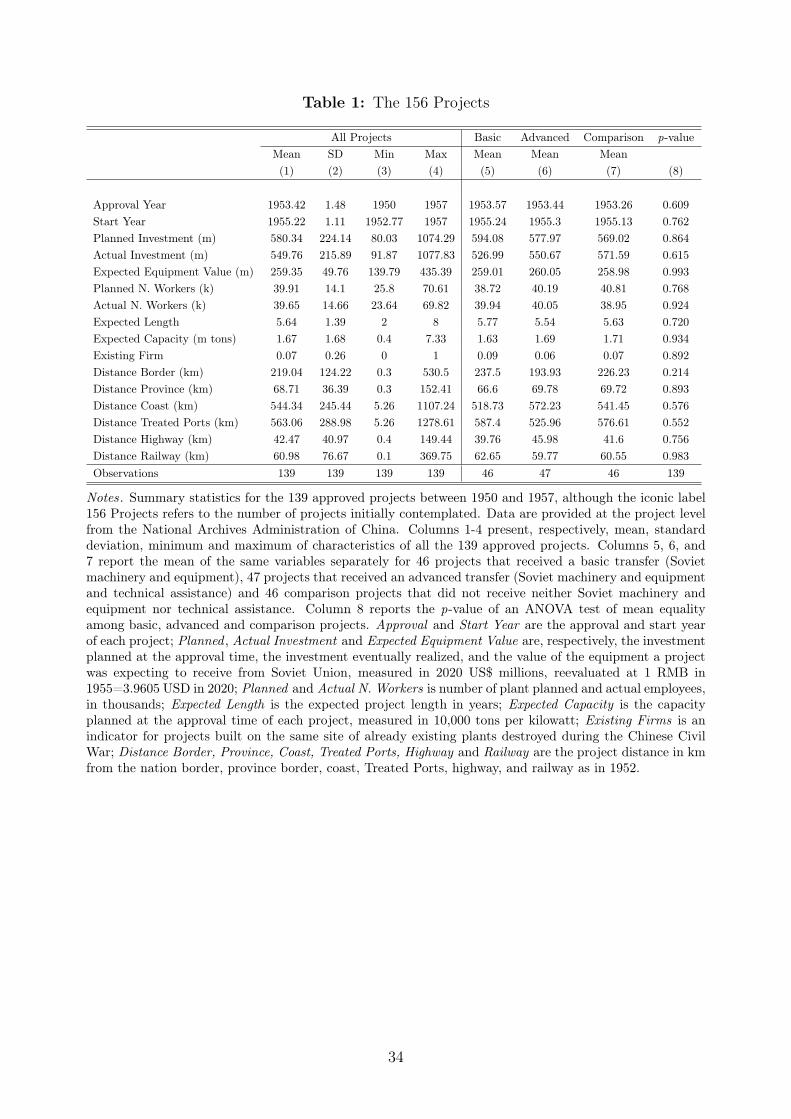
Table 1: The 156 Projects

All Projects Basic Advanced Comparison p-valueMean SD Min Max Mean Mean Mean(1) (2) (3) (4) (5) (6) (7) (8)

Approval Year 1953.42 1.48 1950 1957 1953.57 1953.44 1953.26 0.609Start Year 1955.22 1.11 1952.77 1957 1955.24 1955.3 1955.13 0.762Planned Investment (m) 580.34 224.14 80.03 1074.29 594.08 577.97 569.02 0.864Actual Investment (m) 549.76 215.89 91.87 1077.83 526.99 550.67 571.59 0.615Expected Equipment Value (m) 259.35 49.76 139.79 435.39 259.01 260.05 258.98 0.993Planned N. Workers (k) 39.91 14.1 25.8 70.61 38.72 40.19 40.81 0.768Actual N. Workers (k) 39.65 14.66 23.64 69.82 39.94 40.05 38.95 0.924Expected Length 5.64 1.39 2 8 5.77 5.54 5.63 0.720Expected Capacity (m tons) 1.67 1.68 0.4 7.33 1.63 1.69 1.71 0.934Existing Firm 0.07 0.26 0 1 0.09 0.06 0.07 0.892Distance Border (km) 219.04 124.22 0.3 530.5 237.5 193.93 226.23 0.214Distance Province (km) 68.71 36.39 0.3 152.41 66.6 69.78 69.72 0.893Distance Coast (km) 544.34 245.44 5.26 1107.24 518.73 572.23 541.45 0.576Distance Treated Ports (km) 563.06 288.98 5.26 1278.61 587.4 525.96 576.61 0.552Distance Highway (km) 42.47 40.97 0.4 149.44 39.76 45.98 41.6 0.756Distance Railway (km) 60.98 76.67 0.1 369.75 62.65 59.77 60.55 0.983Observations 139 139 139 139 46 47 46 139

Notes. Summary statistics for the 139 approved projects between 1950 and 1957, although the iconic label156 Projects refers to the number of projects initially contemplated. Data are provided at the project levelfrom the National Archives Administration of China. Columns 1-4 present, respectively, mean, standarddeviation, minimum and maximum of characteristics of all the 139 approved projects. Columns 5, 6, and7 report the mean of the same variables separately for 46 projects that received a basic transfer (Sovietmachinery and equipment), 47 projects that received an advanced transfer (Soviet machinery and equipmentand technical assistance) and 46 comparison projects that did not receive neither Soviet machinery andequipment nor technical assistance. Column 8 reports the p-value of an ANOVA test of mean equalityamong basic, advanced and comparison projects. Approval and Start Year are the approval and start yearof each project; Planned , Actual Investment and Expected Equipment Value are, respectively, the investmentplanned at the approval time, the investment eventually realized, and the value of the equipment a projectwas expecting to receive from Soviet Union, measured in 2020 US$ millions, reevaluated at 1 RMB in1955=3.9605 USD in 2020; Planned and Actual N. Workers is number of plant planned and actual employees,in thousands; Expected Length is the expected project length in years; Expected Capacity is the capacityplanned at the approval time of each project, measured in 10,000 tons per kilowatt; Existing Firms is anindicator for projects built on the same site of already existing plants destroyed during the Chinese CivilWar; Distance Border, Province, Coast, Treated Ports, Highway and Railway are the project distance in kmfrom the nation border, province border, coast, Treated Ports, highway, and railway as in 1952.

34

Table 2: Balancing Tests for Basic, Advanced and Comparison Steel Plants

Mean (1-3) Difference (4-5)Basic Advanced Comparison Basic Advanced(1) (2) (3) (4) (5)

Steel Production (m tons) 604.24 602.06 602.85 2.038 7.022(18.67) (19.43) (23.67) (7.714) (7.669)

Crude Steel Production (m tons) 152.82 153.49 154.62 7.814 -1.293(14.18) (13.98) (14.23) (5.216) (5.678)

Pig Iron Production (m tons) 101.04 96.08 99.31 1.999 0.262(15.70) (15.18) (15.12) (5.393) (5.533)

Current Assets (m) 17.96 17.84 19.10 -0.550 0.458(2.09) (2.82) (2.08) (0.664) (0.903)

Annual Sales (m) 17.18 17.83 18.04 -0.655 0.893(3.56) (3.30) (2.45) (1.146) (1.081)

Value Added (m) 2.53 2.59 2.51 -0.058 0.039(0.27) (0.16) (0.20) (0.112) (0.068)

Productivity (log TFPQ) 1.28 1.21 1.25 0.179 -0.128(0.55) (0.32) (0.25) (0.185) (0.135)

Employees per Plant (k) 6.60 6.49 6.44 0.110 0.242(0.72) (1.03) 0.83 (0.280) (0.296)

Engineers (k) 0.36 0.38 0.37 0.002 0.016(0.05) (0.04) (0.05) (0.021) (0.021)

High-Skilled Technicians (k) 2.17 2.31 2.42 -0.207 -0.104(0.36) (0.14) (0.33) (0.134) (0.095)

Unskilled Workers (k) 3.94 3.9 4.02 -0.156 0.0650.75 1.05 0.91 (0.337) (0.345)

Loans 5.43 5.24 5.09 0.673 0.534(1.86) (0.96) (2.18) (0.587) (0.459)

Transfers 4.37 4.10 3.96 -0.197 -0.274(2.15) (1.05) (2.12) (0.677) (0.502)

Observations 91 98 115 304 304

Notes. Balancing tests for 304 steel plants part belonging to the 156 Projects in the year before receiving theSoviet transfers. Data are provided at plant level from the Steel Association Reports. Columns 1-3 reportmean and standard deviation (in parentheses) of characteristics and outcomes separately for 91 plants whichreceived a basic transfer (Soviet machinery and equipment), 98 plants which received an advanced transfer(Soviet machinery and equipment and technical assistance), and 115 comparison plants that did not receiveneither Soviet machinery and equipment nor technical assistance. Columns 4 and 5 report the coefficientsestimated from regressing each plant variable on an indicator for receiving the basic transfer, an indicatorfor receiving the advanced transfer, and a full set of firm fixed effects (not reported). Steel, Crude Steel andPig Iron Production are the in million tons. Current Assets, Annual Sales and Value Added are measuredin 2020 US$ millions, reevaluated at 1 RMB in 1955=3.9605 USD in 2020; Productivity (logged TFPQ) islogged total factor productivity quantity, computed as log TFPQ = log TFPR� p̃, where ep is the revenue-share weighted average of the prices of plant products, and TFPR is calculated using Gandhi et al. (2020)’smethod; Employees per plant, Engineers, High-Skilled Technicians, and Unskilled Workers are, respectively,thousands of employees, engineers, high-skilled technicians and unskilled workers; Loans and Transfers are,respectively, loans and free transfers that the government granted to each plant, measured in 2020 US$millions, reevaluated at 1 RMB in 1955=3.9605 USD in 2020. Standard errors are clustered at the plantlevel. *** p < 0.01, ** p < 0.05, * p < 0.1. 35

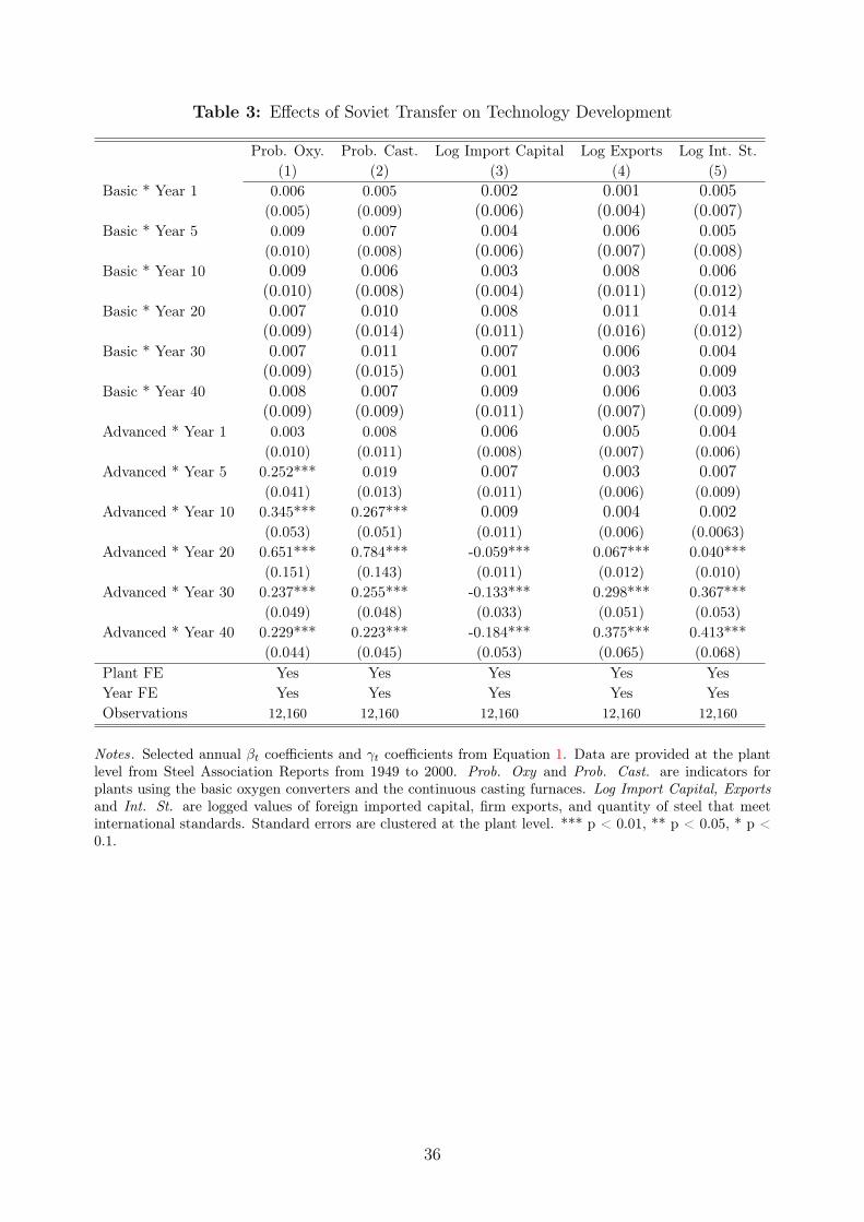
Table 3: Effects of Soviet Transfer on Technology Development

Prob. Oxy. Prob. Cast. Log Import Capital Log Exports Log Int. St.(1) (2) (3) (4) (5)

Basic * Year 1 0.006 0.005 0.002 0.001 0.005(0.005) (0.009) (0.006) (0.004) (0.007)

Basic * Year 5 0.009 0.007 0.004 0.006 0.005(0.010) (0.008) (0.006) (0.007) (0.008)

Basic * Year 10 0.009 0.006 0.003 0.008 0.006(0.010) (0.008) (0.004) (0.011) (0.012)

Basic * Year 20 0.007 0.010 0.008 0.011 0.014(0.009) (0.014) (0.011) (0.016) (0.012)

Basic * Year 30 0.007 0.011 0.007 0.006 0.004(0.009) (0.015) 0.001 0.003 0.009

Basic * Year 40 0.008 0.007 0.009 0.006 0.003(0.009) (0.009) (0.011) (0.007) (0.009)

Advanced * Year 1 0.003 0.008 0.006 0.005 0.004(0.010) (0.011) (0.008) (0.007) (0.006)

Advanced * Year 5 0.252*** 0.019 0.007 0.003 0.007(0.041) (0.013) (0.011) (0.006) (0.009)

Advanced * Year 10 0.345*** 0.267*** 0.009 0.004 0.002(0.053) (0.051) (0.011) (0.006) (0.0063)

Advanced * Year 20 0.651*** 0.784*** -0.059*** 0.067*** 0.040***(0.151) (0.143) (0.011) (0.012) (0.010)

Advanced * Year 30 0.237*** 0.255*** -0.133*** 0.298*** 0.367***(0.049) (0.048) (0.033) (0.051) (0.053)

Advanced * Year 40 0.229*** 0.223*** -0.184*** 0.375*** 0.413***(0.044) (0.045) (0.053) (0.065) (0.068)

Plant FE Yes Yes Yes Yes YesYear FE Yes Yes Yes Yes YesObservations 12,160 12,160 12,160 12,160 12,160

Notes. Selected annual �t coefficients and �t coefficients from Equation 1. Data are provided at the plantlevel from Steel Association Reports from 1949 to 2000. Prob. Oxy and Prob. Cast. are indicators forplants using the basic oxygen converters and the continuous casting furnaces. Log Import Capital, Exportsand Int. St. are logged values of foreign imported capital, firm exports, and quantity of steel that meetinternational standards. Standard errors are clustered at the plant level. *** p < 0.01, ** p < 0.05, * p <0.1.

36

Table 4: Effects of the Soviet Technology Transfer on Steel Plant Human Capital

Log Engineers Log High-Skilled Log Unskilledaaaaaaaaaaaaaaaaaaaaaaaaaaaaaaaaaaaaaaa (1) (2) (3)Basic * Year 5 0.005 -0.003 -0.002

(0.007) (0.005) (0.004)Basic * Year 10 0.006 0.003 -0.009

(0.008) (0.005) (0.014)Basic * Year 20 0.012 0.015 -0.022

(0.018) (0.020) (0.024)Basic * Year 30 0.014 0.011 -0.026

(0.015) (0.010) (0.027)Basic * Year 40 0.009 0.005 -0.013

(0.010) (0.008) (0.016)Advanced*Year 1 0.004 0.005 -0.010

(0.011) (0.012) (0.014)Advanced*Year 5 0.003 -0.005 0.002

(0.007) (0.005) (0.004)Advanced*Year 10 0.026*** 0.028*** -0.045***

(0.007) (0.005) (0.004)Advanced*Year 20 0.043*** 0.038*** -0.080***

(0.007) (0.005) (0.004)Advanced*Year 30 0.063*** 0.045*** -0.101***

(0.007) (0.007) (0.004)Advanced * Year 40 0.085*** 0.058*** -0.133***

(0.007) (0.007) (0.009)Plant FE Yes Yes YesYear FE Yes Yes YesObservations 12,160 12,160 12,160

Notes. Selected annual �t and �t coefficients estimated from Equation 1. Data are provided at the plant levelfrom Steel Association Reports from 1949 to 2000. Log Engineers, High-Skilled, and Unskilled are loggedthousands of engineers, high-skilled technicians, and unskilled employees. Standard errors are clustered atthe plant-level. *** p < 0.01, ** p < 0.05, * p < 0.1.

37

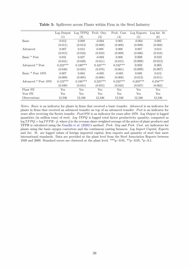
Table 5: Spillovers across Plants within Firm in the Steel Industry

Log Output Log TFPQ Prob. Oxy. Prob. Cast. Log Exports Log Int. St.aaaaaaaaaaa (1) (2) (3) (4) (5) (6)Basic 0.012 0.009 -0.004 0.005 -0.004 0.005

(0.011) (0.013) (0.009) (0.008) (0.009) (0.008)Advanced 0.007 0.012 0.008 0.006 0.007 0.013

(0.015) (0.016) (0.010) (0.009) (0.006) (0.018)Basic * Post 0.031 0.027 -0.003 0.008 0.008 0.010

(0.041) (0.029) (0.011) (0.015) (0.008) (0.013)Advanced * Post 0.223*** 0.199*** 0.425*** 0.532*** 0.002 0.005

(0.049) (0.035) (0.078) (0.061) (0.009) (0.007)Basic * Post 1978 0.007 0.004 -0.005 -0.005 0.009 0.012

(0.009) (0.005) (0.008) (0.008) (0.013) (0.011)Advanced * Post 1978 0.123*** 0.198*** 0.225*** 0.233*** 0.203*** 0.258***

(0.039) (0.041) (0.055) (0.042) (0.047) (0.062)Plant FE Yes Yes Yes Yes Yes YesYear FE Yes Yes Yes Yes Yes YesObservations 12,346 12,346 12,346 12,346 12,346 12,346

Notes. Basic is an indicator for plants in firms that received a basic transfer. Advanced is an indicator forplants in firms that received an advanced transfer on top of an advanced transfer. Post is an indicator foryears after receiving the Soviet transfer. Post1978 is an indicator for years after 1978. Log Output is loggedquantities (in million tons) of steel. Log TFPQ is logged total factor productivity quantity, computed aslog TFPQ = log TFPR�p̃, where ep is the revenue share weighted average of the prices of plant products andTFPR is calculated using the Gandhi et al. (2020)’s method. Prob. Oxy and Prob. Cast. are indicators forplants using the basic oxygen converters and the continuous casting furnaces. Log Import Capital, Exportsand Int. St. are logged values of foreign imported capital, firm exports and quantity of steel that meetinternational standards. Data are provided at the plant level from the Steel Association Reports between1949 and 2000. Standard errors are clustered at the plant level. ***p<0.01, **p<0.05, *p<0.1.

38

Table 6: Horizontal Spillovers in the Steel Industry

Log Output Log TFPQ Prob. Oxy. Prob. Cast. Log Exports Log Int. St.aaaaaaaaaaa (1) (2) (3) (4) (5) (6)Basic -0.018 -0.016 -0.009 0.007 0.008 0.009

(0.022) (0.038) (0.010) (0.011) (0.010) (0.012)Advanced 0.012 0.014 0.006 0.011 0.005 0.006

(0.014) (0.016) (0.008) (0.015) (0.007) (0.009)Basic * Post 0.006 0.011 0.009 0.012 0.007 0.012

(0.008) (0.015) (0.010) (0.013) (0.011) (0.013)Advanced * Post 0.122*** 0.117*** 0.308*** 0.319*** 0.016 0.019

(0.017) (0.015) (0.111) (0.123) 0.011) (0.016)Basic * Post 1978 -0.015 0.022 0.004 0.006 0.005 0.009

(0.020) (0.021) (0.010) (0.011) (0.008) (0.012)Advanced * Post 1978 0.022*** 0.018*** 0.033*** 0.045*** 0.187*** 0.201***

(0.007) (0.006) (0.012) (0.009) (0.051) (0.065)Plant FE Yes Yes Yes Yes Yes YesYear FE Yes Yes Yes Yes Yes YesObservations 13,550 13,550 13,550 13,550 13,550 13,550

Notes. Basic is an indicator for steel plants in the same counties of steel plants that received a basictransfer. Advanced is an indicator for steel plants in the same counties of steel plants that received anadvanced transfer on top of a basic transfer. Post is an indicator for years after receiving the Soviettransfer. Post1978 is an indicator for years after 1978. Log Output is logged quantities (in million tons)of steel. Log TFPQ is logged total factor productivity quantity, computed as log TFPQ = log TFPR � p̃,where ep is the revenue share weighted average of the prices of plant products and TFPR is calculated usingthe Gandhi et al. (2020)’s method. Prob. Oxy and Prob. Cast. are indicators for plants using the basicoxygen converters and the continuous casting furnaces. Log Import Capital, Exports and Int. St. are loggedvalues of foreign imported capital, firm exports and quantity of steel that meet international standards.Data are provided at the plant level from the Steel Association Reports between 1949 and 2000. Standarderrors are clustered at the plant level. ***p<0.01, **p<0.05, *p<0.1.

Table 7: Vertical Spillover Effects in the Steel Industry

Log Output Log TFPQ Prob. Oxy. Prob. Cast. Log Exports Log Int. St.aaaaaaaaaaa (1) (2) (3) (4) (5) (6)Basic 0.008 0.004 0.005 0.006 0.004 0.007

(0.011) (0.006) (0.007) (0.010) (0.009) (0.010)Advanced 0.003 0.009 0.004 0.009 0.005 0.006

(0.004) (0.006) (0.005) (0.010) (0.008) (0.009)Basic * Post 0.133*** 0.011 0.009 0.006 0.016 0.012

(0.022) (0.014) (0.011) (0.009) (0.015) (0.016)Advanced * Post 0.152*** 0.132*** 0.106*** 0.100*** 0.004 0.006

(0.035) (0.039) (0.031) (0.025) (0.005) (0.009)Basic * Post 1978 -0.015 0.022 0.004 0.006 0.009 0.011

(0.020) (0.021) (0.010) (0.011) (0.010) (0.025)Advanced * Post 1978 0.034*** 0.028*** 0.029*** 0.037*** 0.145*** 0.138***

(0.008) (0.007) (0.008) (0.006) (0.032) (0.031)County-Year FE Yes Yes Yes Yes Yes YesObservations 15,340 15,340 15,340 15,340 15,340 15,340

Notes. Basic is an indicator for steel plants in the same counties of nonsteel plants that received a basictransfer. Advanced is an indicator for steel plants in the same counties of nonsteel plants that received anadvanced transfer on top of an advanced transfer. Post is an indicator for years after receiving the Soviettransfer. Post1978 is an indicator for years after 1978. Log Output is logged quantities (in million tons)of steel. Log TFPQ is logged total factor productivity quantity, computed as log TFPQ = log TFPR � p̃,where ep is the revenue share weighted average of the prices of plant products and TFPR is calculated usingthe Gandhi et al. (2020)’s method. Prob. Oxy and Prob. Cast. are indicators for plants using the basicoxygen converters and the continuous casting furnaces. Log Import Capital, Exports and Int. St. are loggedvalues of foreign imported capital, firm exports and quantity of steel that meet international standards.Data are provided at the plant level from the Steel Association Reports between 1949 and 2000. Standarderrors are clustered at the plant level. ***p<0.01, **p<0.05, *p<0.1.

39

Table 8: Spillover Effects, 1998–2013

Log Value Added Log TFPR Log Exportsaaaaaaaaaaaaaaaa (1) (2) (3) (4) (5) (6)Panel A: Related FirmsBasic 0.013 0.010 -0.005 -0.003 -0.012 -0.010

(0.025) (0.020) (0.018) (0.009) (0.015) (0.012)Advanced 0.011 -0.009 0.003 0.004 0.008 -0.015

(0.020) (0.012) (0.008) (0.004) (0.007) (0.018)Basic * Private 0.022 0.020 0.025 0.021 0.008 0.004

(0.031) (0.029) (0.028) (0.0283) (0.013) (0.003)Advanced * Private 0.215*** 0.206*** 0.209*** 0.200*** 0.134*** 0.124***

(0.031) (0.044) (0.045) (0.041) (0.033) (0.028)Basic * Private * New 0.015 0.011 0.019 0.021 0.023 0.016

(0.018) (0.017) (0.026) (0.024) (0.022) (0.021)Advanced * Private * New 0.033*** 0.030*** 0.031*** 0.025*** 0.050*** 0.044***

(0.011) (0.009) (0.006) (0.005) (0.012) (0.010)Sector-Province-Year FE Yes No Yes No Yes NoSector-Prefecture-Year FE No Yes No Yes No YesObservations 160,123 160,123 160,123 160,123 160,123 160,123

Panel B: Not Related FirmsBasic 0.012 -0.004 -0.003 -0.015 -0.005 -0.004

(0.015) (0.011) (0.018) (0.016) (0.012) (0.009)Advanced 0.004 -0.003 0.004 0.003 0.003 -0.002

(0.006) (0.006) (0.008) (0.007) (0.005) (0.004)Basic * Private 0.005 -0.004 -0.004 0.008 -0.005 -0.003

(0.005) (0.012) (0.007) (0.011) (0.008) (0.005)Advanced * Private 0.002 0.005 0.003 -0.004 0.001 0.007

(0.006) (0.010) (0.004) (0.005) (0.002) (0.008)Basic * Private * New 0.002 0.005 -0.002 -0.003 0.003 0.001

(0.006) (0.008) (0.005) (0.009) (0.005) (0.003)Advanced * Private * New -0.008 -0.003 0.005 -0.006 0.006 0.003

(0.010) (0.004) (0.005) (0.009) (0.009) (0.038)Sector-Province-Year FE Yes No Yes No Yes NoSector-Prefecture-Year FE No Yes No Yes No YesObservations 124,762 124,762 124,762 124,762 124,762 124,762

Notes. Basic in an indicator for counties where plants that received a basic transfer were located. Advancedin an indicator for counties where plants that received an advanced transfer were located. Private is anindicator equal to one for non-state-owned firms. New is an indicator equal to one for firms that enteredthe market between 1998 and 2013. Log Value Added and Exports are measured in 2020 US$ millions,reevaluated at 1 RMB in 1955=3.9605 USD in 2020; Log TFPR is logged total factor productivity revenuecomputed with Gandhi et al. (2020) method. Data are provided at the firm level from the China IndustrialEnterprises database between 1998 and 2013. Standard errors are clustered at the firm level. *** p < 0.01,** p < 0.05, * p < 0.1.

40

Online Appendix — Not for Publication

Additional Figures and Tables

Figure A.1: The 156 Projects by Industry

23.021.6

20.1

14.4

10.1

5.0

2.2 2.2 1.4

05

1015

2025

Perc

enta

ge o

f Pro

ject

s

Electric

ity

Machin

eries Coa

lStee

l

Non-Ferr

ous M

etals

Chemica

ls

Pharm

aceu

tical Oil

Light

Indus

try

Notes. Distribution of the 139 approved technology transfer projects by industry, although 156 projects wereinitially contemplated. Data are provided at the project level from the National Archives Administration ofChina.

A1

Figure A.2: Industry Dynamics

Panel A: By Sector

Panel B: By Industry

Notes. Panel A shows the percentage of firms in the agriculture, manufacturing, and heavy industries,respectively, from 1949 to 1985. Panel B shows the detailed industry distribution in heavy industries(metallurgy, chemicals, and machinery), and manufacturing-related industries (wood, textile, food). Dataare provided at the province level from the Statistical Yearbooks between 1949 and 1985.

A2

Figure A.3: Ownership and Regional Allocation

Panel A: Ownership Allocation

Panel B: Regional Allocation

Notes. Panel A shows changes in the percentage of firms operating as state-owned, collective, public-private,private, and individual firms, respectively, from 1949 to 1985. Panel B displays the production allocationbetween coastal regions and inland regions. Data are provided at the province level from the StatisticalYearbooks between 1949 and 1985.

A3

Figure A.4: Probability of Receiving the Soviet Technology Transfer, by Prefectures andCounties

Panel A: Prefectures

p-value χ2=0.651

-1-.5

0.5

1Pr

edic

ted

Prob

abilit

y

Beijing

Ansha

n

Baodin

g

BaotouBen

xi

Chang

chun

Cheng

de

Cheng

du

Chong

qing

Dalian

Datong

Dngch

uan

Fushu

nFux

in

Ganzh

ou

Handa

nHarb

in

Hegan

g

Hejiang

Hongh

e

Huaina

n

Huang

shi

Jiaoz

uoJilin

Jinzh

ou

Jiuqu

anJixi

Lanz

hou

Luoy

ang

Luoy

ang

Pingdin

gsha

n

Qjqihar

Qujing

Sheny

ang

Shijizh

uan

Shuan

gyas

han

Siping

Southe

aster

n Sha

nxi

Taiyu

an

Tong

chua

n

Tong

hua

WuhanXian

Xiangta

n

Xianya

ngYan

bei

Yingko

u

Yueya

ng

Zhang

ye

Zheng

zhou

Zhuzh

ou

Advanced Transfer Basic Transfer

Panel B: Counties

p-value χ2=0.498

-1-.5

0.5

1Pr

edic

ted

Prob

abilit

y

Chaoy

ang

Baiyin

Baodin

g

BaqiaoBeili

nBen

xi

Chang

shou

Chang

yi

ChengChe

ng

Cheng

de

Cheng

guan

Cheng

zihe

Daduk

ouDay

eDay

u

Dingna

n

Dongc

huan

Dongs

han

Dongx

ihu

East D

istrict

Fengfe

ng

Fulaerj

iGejiu

Handa

nHex

i

Hongs

han

Huaire

n

Huluda

o

Huxian

Jiamus

i

Jiang

an

Jians

han

Jianx

i

Jiao D

istrict

B.

Jiao D

istrict

Jia

Jiao D

istrict

Jil.

Jiao D

istrict

S.

Jingx

ingJin

niu

Jiulon

gpo

Kaiyua

n

Kundu

lunLia

nhu

Liaoy

uan

Long

tanLu

tian

Nangu

an

Nanjiao

North D

istrict

Qingsh

an

Qingsh

an

Quann

anQujin

g

Sanmen

xia

Shuan

gluan

Shuim

ogou

South

District

Taipin

g

Tiexi A

.

Tiexi S

.

Tong

hua

Wangh

ua

Wucha

ng

Xiangfr

ang

Xiangy

uan

Xiejiaji

XigangXigu

XinbinXinf

u

Xingan

XinhuaXinq

iu

Yong

deng

Yuetan

g

Yuetan

g

Yugua

n

Yuzho

ng

Zhang

wu

Zhingy

uan

Advanced Transfer Basic Transfer

Notes. Predicted probabilities (marginal effects) of receiving a basic or an advanced transfer relative to thebaseline of not receiving any Soviet transfer and 95% confidence intervals, estimated from the multinominallogit log

� Pr(Transferi=j)Pr(Comparisoni)

�= ↵ + !p + ✏i in Panel A and from the multinominal logit log

� Pr(Transferi=j)Pr(Comparisoni)

�=

↵ + �c + ⌫i in Panel B, where !p are project prefecture city fixed effects and �c are project county fixedeffects. p-values of �2 test of joint equality of all coefficients to zero are reported in each panel. Data areprovided at the project level from the National Archives Administration of China.

A4

Table A.1: Pre-Technology Transfer Differences in Counties Hosting Basic, Advancedand Comparison Plants in 1953

Log Total Firms Log Population Employment Share Log Gvt. Funds(1) (2) (3) (4)

Basic 0.018 -0.013 0.006 0.003(0.013) (0.011) (0.014) (0.006)

Advanced -0.015 0.012 0.004 0.007(0.016) (0.013) (0.011) (0.012)

Observations 81 81 81 81

Notes. OLS regressions predicting county-level outcomes in 1953. Data are provided at county-level fromthe People’s Republic of China Population Digest in 1953. Log total firms is logged total number of firms percounty; Log population is logged total population of a county; Employment Share is the fraction of employedpopulation over total population; Log Gvt. Funds is logged free transfers that the government granted tocounty, measured in 2020 US$ millions, reevaluated at 1 RMB in 1955=3.9605 USD in 2020. Basic is anindicator for counties where plants that received a basic transfer were located. Advanced is an indicator forcounties where plants that received an advanced transfer were located. *** p < 0.01, ** p < 0.05, * p <0.1.

A5

Table A.2: Pre-Soviet Technology Transfer Difference in Time Trends in Basic, Advancedand Comparison Steel Plants

Log Steel Log Crude Steel Log Pig Iron Log Current Assets(1) (2) (3) (4) (5) (6) (7) (8)

Basic * Trend -0.001 -0.002 0.006 0.007 -0.004 -0.007 0.002 0.002(0.001) (0.003) (0.009) (0.008) (0.004) (0.009) (0.003) (0.004)

Advanced * Trend 0.005 0.004 0.002 -0.002 -0.005 -0.003 -0.003 -0.005(0.008) (0.007) (0.003) (0.004) (0.007) (0.004) (0.004) (0.008)

Time Trend -0.009 -0.003 -0.002 -0.003 -0.004 -0.005 0.009 -0.003(0.010) (0.004) (0.002) (0.006) (0.006) (0.008) (0.012) (0.006)

Basic 0.003 0.003 -0.005 -0.007 0.007 0.006 -0.005 -0.014(0.006) (0.003) (0.009) (0.015) (0.015) (0.014) (0.011) (0.018)

Advanced 0.005 -0.002 -0.012 -0.009 -0.012 -0.011 -0.007 -0.004(0.005) (0.003) (0.010) (0.016) (0.016) (0.017) (0.014) (0.012)Log Annual Sales Log Value Added Log TFPQ Log Employees

Basic * Trend -0.002 -0.003 0.002 0.005 -0.002 -0.003 -0.006 -0.004(0.005) (0.004) (0.003) (0.010) (0.012) (0.009) (0.008) (0.006)

Advanced * Trend 0.002 0.006 0.001 0.001 -0.016 -0.014 0.009 0.010(0.005) (0.008) (0.002) (0.002) (0.017) (0.018) (0.010) (0.011)

Time Trend 0.002 -0.001 -0.002 -0.002 -0.004 -0.002 -0.002 -0.003(0.003) (0.002) (0.001) (0.004) (0.005) (0.003) (0.005) (0.006)

Basic -0.005 0.012 -0.014 -0.015 -0.007 -0.009 0.010 0.008(0.017) (0.013) (0.012) (0.015) (0.006) (0.008) (0.011) (0.012)

Advanced -0.015 -0.016 0.013 0.018 -0.013 0.009 0.016 0.013(0.016) (0.017) (0.017) (0.016) (0.016) (0.011) (0.014) (0.012)

Log Engineers Log High-Skilled Log Loans Log TransfersBasic * Trend 0.002 0.005 0.007 0.007 -0.004 -0.003 0.013 0.013

(0.004) (0.008) (0.009) (0.014) (0.006) (0.004) (0.016) (0.016)Advanced * Trend -0.002 -0.004 0.004 0.005 -0.003 -0.007 0.014 0.014

(0.004) (0.005) (0.003) (0.007) (0.011) (0.010) (0.011) (0.011)Time Trend -0.005 -0.006 -0.003 -0.002 0.001 0.002 -0.013 -0.015

(0.009) (0.008) (0.003) (0.002) (0.010) (0.009) (0.011) (0.010)Basic -0.009 -0.014 -0.011 -0.012 0.017 0.018 0.004 -0.011

(0.014) (0.015) (0.015) (0.017) (0.018) (0.019) (0.005) (0.009)Advanced 0.018 0.019 -0.013 -0.012 0.010 0.016 0.007 0.013

(0.013) (0.023) (0.011) (0.013) (0.012) (0.016) (0.012) (0.016)Observations 2,114 2,114 2,114 2,114 2,114 2,114 2,114 2,114Plant FE Yes No Yes No Yes No Yes NoPlant x Year FE No Yes No Yes No Yes No Yes

Notes. OLS regressions predicting plant outcomes before receiving the Soviet transfer. Data are providedat plant level from the Steel Association Reports. Outcomes are allowed to vary according to a linear timetrend that differs for plants that received a basic transfer (Soviet machinery and equipment) and for plantsthat received an advanced transfer (Soviet machinery and equipment and technical assistance). Steel, CrudeSteel and Pig Iron Production are the in million tons. Current Assets, Annual Sales and Value Added aremeasured in 2020 US$ millions, reevaluated at 1 RMB in 1955=3.9605 USD in 2020; Productivity (loggedTFPQ) is logged total factor productivity quantity, computed as log TFPQ = log TFPR� p̃, where ep is therevenue-share weighted average of the prices of plant products, and TFPR is calculated using Gandhi et al.(2020)’s method; Employees per plant, Engineers, and High-Skilled Technicians are, respectively, thousandsof employees, engineers, and high-skilled technicians; Loans and Transfers are, respectively, loans and freetransfers that the government granted to each plant, measured in 2020 US$ millions, reevaluated at 1 RMBin 1955=3.9605 USD in 2020. Standard errors are clustered at the plant level. *** p < 0.01, ** p < 0.05, *p < 0.1.

A6

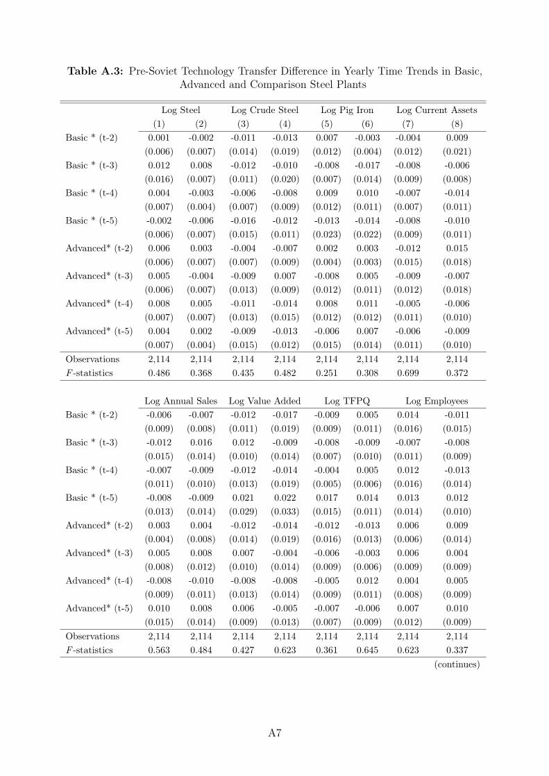
Table A.3: Pre-Soviet Technology Transfer Difference in Yearly Time Trends in Basic,Advanced and Comparison Steel Plants

Log Steel Log Crude Steel Log Pig Iron Log Current Assets(1) (2) (3) (4) (5) (6) (7) (8)

Basic * (t-2) 0.001 -0.002 -0.011 -0.013 0.007 -0.003 -0.004 0.009(0.006) (0.007) (0.014) (0.019) (0.012) (0.004) (0.012) (0.021)

Basic * (t-3) 0.012 0.008 -0.012 -0.010 -0.008 -0.017 -0.008 -0.006(0.016) (0.007) (0.011) (0.020) (0.007) (0.014) (0.009) (0.008)

Basic * (t-4) 0.004 -0.003 -0.006 -0.008 0.009 0.010 -0.007 -0.014(0.007) (0.004) (0.007) (0.009) (0.012) (0.011) (0.007) (0.011)

Basic * (t-5) -0.002 -0.006 -0.016 -0.012 -0.013 -0.014 -0.008 -0.010(0.006) (0.007) (0.015) (0.011) (0.023) (0.022) (0.009) (0.011)

Advanced* (t-2) 0.006 0.003 -0.004 -0.007 0.002 0.003 -0.012 0.015(0.006) (0.007) (0.007) (0.009) (0.004) (0.003) (0.015) (0.018)

Advanced* (t-3) 0.005 -0.004 -0.009 0.007 -0.008 0.005 -0.009 -0.007(0.006) (0.007) (0.013) (0.009) (0.012) (0.011) (0.012) (0.018)

Advanced* (t-4) 0.008 0.005 -0.011 -0.014 0.008 0.011 -0.005 -0.006(0.007) (0.007) (0.013) (0.015) (0.012) (0.012) (0.011) (0.010)

Advanced* (t-5) 0.004 0.002 -0.009 -0.013 -0.006 0.007 -0.006 -0.009(0.007) (0.004) (0.015) (0.012) (0.015) (0.014) (0.011) (0.010)

Observations 2,114 2,114 2,114 2,114 2,114 2,114 2,114 2,114F -statistics 0.486 0.368 0.435 0.482 0.251 0.308 0.699 0.372

Log Annual Sales Log Value Added Log TFPQ Log EmployeesBasic * (t-2) -0.006 -0.007 -0.012 -0.017 -0.009 0.005 0.014 -0.011

(0.009) (0.008) (0.011) (0.019) (0.009) (0.011) (0.016) (0.015)Basic * (t-3) -0.012 0.016 0.012 -0.009 -0.008 -0.009 -0.007 -0.008

(0.015) (0.014) (0.010) (0.014) (0.007) (0.010) (0.011) (0.009)Basic * (t-4) -0.007 -0.009 -0.012 -0.014 -0.004 0.005 0.012 -0.013

(0.011) (0.010) (0.013) (0.019) (0.005) (0.006) (0.016) (0.014)Basic * (t-5) -0.008 -0.009 0.021 0.022 0.017 0.014 0.013 0.012

(0.013) (0.014) (0.029) (0.033) (0.015) (0.011) (0.014) (0.010)Advanced* (t-2) 0.003 0.004 -0.012 -0.014 -0.012 -0.013 0.006 0.009

(0.004) (0.008) (0.014) (0.019) (0.016) (0.013) (0.006) (0.014)Advanced* (t-3) 0.005 0.008 0.007 -0.004 -0.006 -0.003 0.006 0.004

(0.008) (0.012) (0.010) (0.014) (0.009) (0.006) (0.009) (0.009)Advanced* (t-4) -0.008 -0.010 -0.008 -0.008 -0.005 0.012 0.004 0.005

(0.009) (0.011) (0.013) (0.014) (0.009) (0.011) (0.008) (0.009)Advanced* (t-5) 0.010 0.008 0.006 -0.005 -0.007 -0.006 0.007 0.010

(0.015) (0.014) (0.009) (0.013) (0.007) (0.009) (0.012) (0.009)Observations 2,114 2,114 2,114 2,114 2,114 2,114 2,114 2,114F -statistics 0.563 0.484 0.427 0.623 0.361 0.645 0.623 0.337

(continues)

A7

Table A.3: Continued

Log Engineers Log High-Skilled Log Loans Log TransfersBasic * (t-2) -0.009 0.015 -0.007 -0.013 -0.018 0.010 -0.007 -0.009

(0.013) (0.030) (0.013) (0.012) (0.013) (0.014) (0.006) (0.014)Basic * (t-3) 0.013 0.022 -0.005 0.005 0.017 0.011 0.009 0.010

(0.019) (0.027) (0.007) (0.007) (0.015) (0.009) (0.016) (0.011)Basic * (t-4) -0.014 0.020 -0.011 -0.004 0.007 0.012 0.009 -0.011

(0.020) (0.028) (0.012) (0.009) (0.006) (0.010) (0.009) (0.009)Basic * (t-5) 0.011 0.012 -0.009 -0.011 0.006 0.008 0.015 0.020

(0.018) (0.015) (0.011) (0.015) (0.006) (0.007) (0.014) (0.018)Advanced* (t-2) -0.016 0.018 -0.010 0.013 0.004 0.009 0.008 0.006

(0.019) (0.018) (0.012) (0.015) (0.0607) (0.010) (0.010) (0.007)Advanced* (t-3) 0.015 0.014 -0.019 0.011 0.016 0.012 0.008 0.009

(0.020) (0.017) (0.020) (0.015) (0.018) (0.016) (0.009) (0.010)Advanced* (t-4) -0.014 -0.015 -0.003 -0.004 0.008 0.007 0.012 0.010

(0.020) (0.016) (0.005) (0.009) (0.008) (0.009) (0.015) (0.012)Advanced* (t-5) 0.007 -0.004 -0.009 0.011 0.012 0.009 0.012 -0.013

(0.011) (0.006) (0.014) (0.020) (0.013) (0.010) (0.016) (0.010)Observations 2,114 2,114 2,114 2,114 2,114 2,114 2,114 2,114F -statistics 0.709 0.295 0.337 0.438 0.380 0.659 0.410 0.413

Notes. OLS regressions predicting plant outcomes before in the five years before receiving the Soviet transfer.Data are provided at plant level from the Steel Association Reports. The trend is allowed to vary freelyfor each year before receiving the Soviet transfer for plants that received a basic transfer (Soviet machineryand equipment) and for plants that received an advanced transfer (Soviet machinery and equipment andtechnical assistance). Time period indicators are included, but not reported. The omitted period is t=-1,the year before receiving the Soviet transfer. Steel, Crude Steel and Pig Iron Production are the in milliontons. Current Assets, Annual Sales and Value Added are measured in 2020 US$ millions, reevaluated at 1RMB in 1955=3.9605 USD in 2020; Productivity (logged TFPQ) is logged total factor productivity quantity,computed as log TFPQ = log TFPR�p̃, where ep is the revenue-share weighted average of the prices of plantproducts, and TFPR is calculated using Gandhi et al. (2020)’s method; Employees per plant, Engineers, andHigh-Skilled Technicians are, respectively, thousands of employees, engineers, and high-skilled technicians;Loans and Transfers are, respectively, loans and free transfers that the government granted to each plant,measured in 2020 US$ millions, reevaluated at 1 RMB in 1955=3.9605 USD in 2020. Standard errors areclustered at the plant level. *** p < 0.01, ** p < 0.05, * p < 0.1. The F -statistics test whether all theinteraction terms between basic and advanced plants and the year indicators are jointly zero.

A8

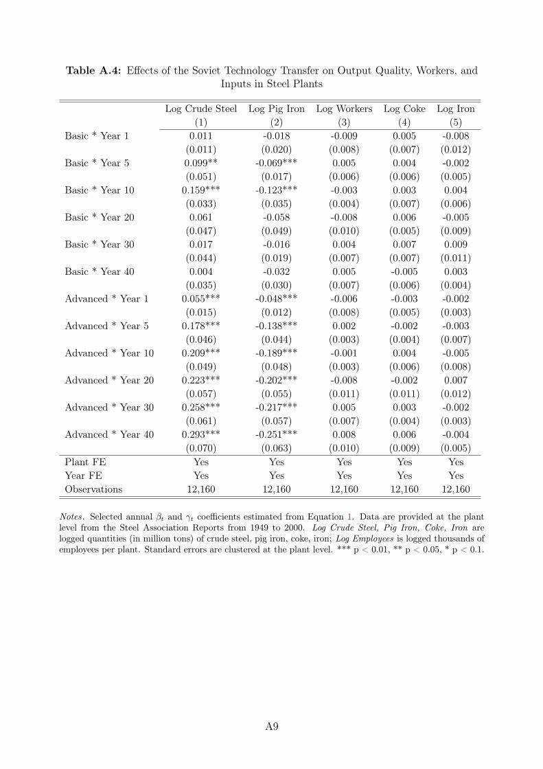
Table A.4: Effects of the Soviet Technology Transfer on Output Quality, Workers, andInputs in Steel Plants

Log Crude Steel Log Pig Iron Log Workers Log Coke Log Iron(1) (2) (3) (4) (5)

Basic * Year 1 0.011 -0.018 -0.009 0.005 -0.008(0.011) (0.020) (0.008) (0.007) (0.012)

Basic * Year 5 0.099** -0.069*** 0.005 0.004 -0.002(0.051) (0.017) (0.006) (0.006) (0.005)

Basic * Year 10 0.159*** -0.123*** -0.003 0.003 0.004(0.033) (0.035) (0.004) (0.007) (0.006)

Basic * Year 20 0.061 -0.058 -0.008 0.006 -0.005(0.047) (0.049) (0.010) (0.005) (0.009)

Basic * Year 30 0.017 -0.016 0.004 0.007 0.009(0.044) (0.019) (0.007) (0.007) (0.011)

Basic * Year 40 0.004 -0.032 0.005 -0.005 0.003(0.035) (0.030) (0.007) (0.006) (0.004)

Advanced * Year 1 0.055*** -0.048*** -0.006 -0.003 -0.002(0.015) (0.012) (0.008) (0.005) (0.003)

Advanced * Year 5 0.178*** -0.138*** 0.002 -0.002 -0.003(0.046) (0.044) (0.003) (0.004) (0.007)

Advanced * Year 10 0.209*** -0.189*** -0.001 0.004 -0.005(0.049) (0.048) (0.003) (0.006) (0.008)

Advanced * Year 20 0.223*** -0.202*** -0.008 -0.002 0.007(0.057) (0.055) (0.011) (0.011) (0.012)

Advanced * Year 30 0.258*** -0.217*** 0.005 0.003 -0.002(0.061) (0.057) (0.007) (0.004) (0.003)

Advanced * Year 40 0.293*** -0.251*** 0.008 0.006 -0.004(0.070) (0.063) (0.010) (0.009) (0.005)

Plant FE Yes Yes Yes Yes YesYear FE Yes Yes Yes Yes YesObservations 12,160 12,160 12,160 12,160 12,160

Notes. Selected annual �t and �t coefficients estimated from Equation 1. Data are provided at the plantlevel from the Steel Association Reports from 1949 to 2000. Log Crude Steel, Pig Iron, Coke, Iron arelogged quantities (in million tons) of crude steel, pig iron, coke, iron; Log Employees is logged thousands ofemployees per plant. Standard errors are clustered at the plant level. *** p < 0.01, ** p < 0.05, * p < 0.1.

A9

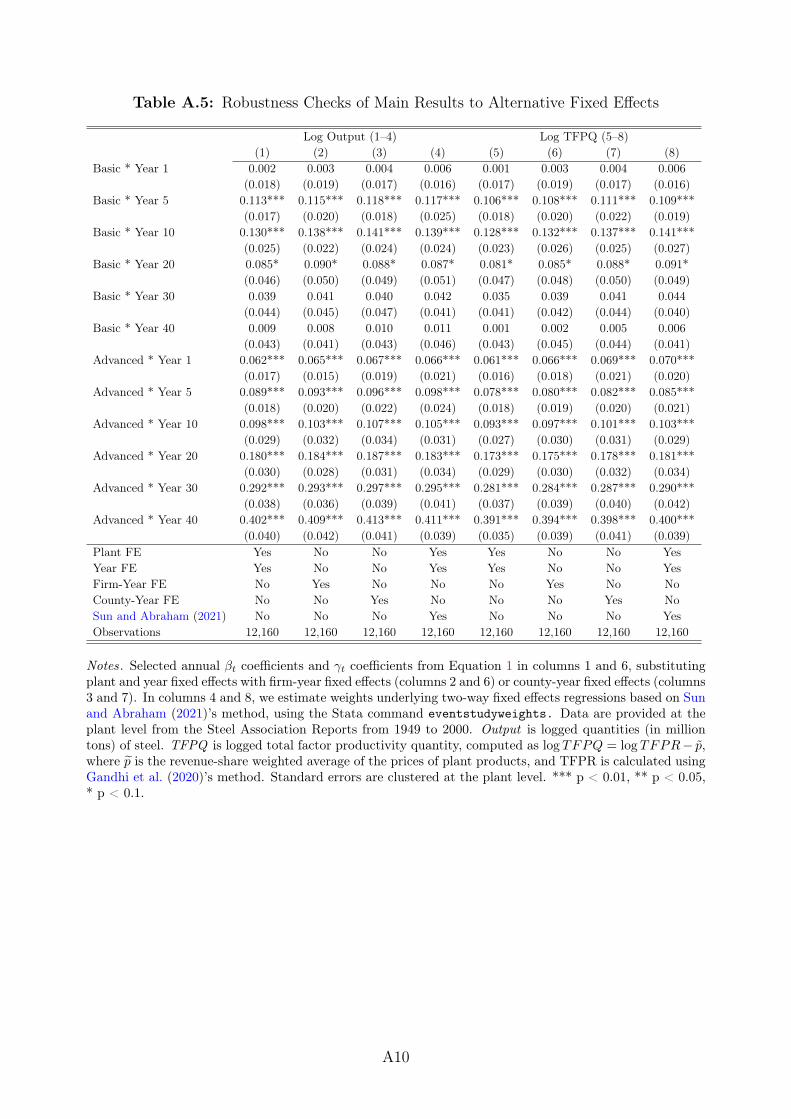
Table A.5: Robustness Checks of Main Results to Alternative Fixed Effects

Log Output (1–4) Log TFPQ (5–8)(1) (2) (3) (4) (5) (6) (7) (8)

Basic * Year 1 0.002 0.003 0.004 0.006 0.001 0.003 0.004 0.006(0.018) (0.019) (0.017) (0.016) (0.017) (0.019) (0.017) (0.016)

Basic * Year 5 0.113*** 0.115*** 0.118*** 0.117*** 0.106*** 0.108*** 0.111*** 0.109***(0.017) (0.020) (0.018) (0.025) (0.018) (0.020) (0.022) (0.019)

Basic * Year 10 0.130*** 0.138*** 0.141*** 0.139*** 0.128*** 0.132*** 0.137*** 0.141***(0.025) (0.022) (0.024) (0.024) (0.023) (0.026) (0.025) (0.027)

Basic * Year 20 0.085* 0.090* 0.088* 0.087* 0.081* 0.085* 0.088* 0.091*(0.046) (0.050) (0.049) (0.051) (0.047) (0.048) (0.050) (0.049)

Basic * Year 30 0.039 0.041 0.040 0.042 0.035 0.039 0.041 0.044(0.044) (0.045) (0.047) (0.041) (0.041) (0.042) (0.044) (0.040)

Basic * Year 40 0.009 0.008 0.010 0.011 0.001 0.002 0.005 0.006(0.043) (0.041) (0.043) (0.046) (0.043) (0.045) (0.044) (0.041)

Advanced * Year 1 0.062*** 0.065*** 0.067*** 0.066*** 0.061*** 0.066*** 0.069*** 0.070***(0.017) (0.015) (0.019) (0.021) (0.016) (0.018) (0.021) (0.020)

Advanced * Year 5 0.089*** 0.093*** 0.096*** 0.098*** 0.078*** 0.080*** 0.082*** 0.085***(0.018) (0.020) (0.022) (0.024) (0.018) (0.019) (0.020) (0.021)

Advanced * Year 10 0.098*** 0.103*** 0.107*** 0.105*** 0.093*** 0.097*** 0.101*** 0.103***(0.029) (0.032) (0.034) (0.031) (0.027) (0.030) (0.031) (0.029)

Advanced * Year 20 0.180*** 0.184*** 0.187*** 0.183*** 0.173*** 0.175*** 0.178*** 0.181***(0.030) (0.028) (0.031) (0.034) (0.029) (0.030) (0.032) (0.034)

Advanced * Year 30 0.292*** 0.293*** 0.297*** 0.295*** 0.281*** 0.284*** 0.287*** 0.290***(0.038) (0.036) (0.039) (0.041) (0.037) (0.039) (0.040) (0.042)

Advanced * Year 40 0.402*** 0.409*** 0.413*** 0.411*** 0.391*** 0.394*** 0.398*** 0.400***(0.040) (0.042) (0.041) (0.039) (0.035) (0.039) (0.041) (0.039)

Plant FE Yes No No Yes Yes No No YesYear FE Yes No No Yes Yes No No YesFirm-Year FE No Yes No No No Yes No NoCounty-Year FE No No Yes No No No Yes NoSun and Abraham (2021) No No No Yes No No No YesObservations 12,160 12,160 12,160 12,160 12,160 12,160 12,160 12,160

Notes. Selected annual �t coefficients and �t coefficients from Equation 1 in columns 1 and 6, substitutingplant and year fixed effects with firm-year fixed effects (columns 2 and 6) or county-year fixed effects (columns3 and 7). In columns 4 and 8, we estimate weights underlying two-way fixed effects regressions based on Sunand Abraham (2021)’s method, using the Stata command eventstudyweights. Data are provided at theplant level from the Steel Association Reports from 1949 to 2000. Output is logged quantities (in milliontons) of steel. TFPQ is logged total factor productivity quantity, computed as log TFPQ = log TFPR� p̃,where ep is the revenue-share weighted average of the prices of plant products, and TFPR is calculated usingGandhi et al. (2020)’s method. Standard errors are clustered at the plant level. *** p < 0.01, ** p < 0.05,* p < 0.1.

A10

Table A.6: Robustness Checks of Main Results to Alternative Timing

Log Output (1–3) Log TFPQ (4–6)(1) (2) (3) (4) (5) (6)

Basic * Year 1 0.002 0.002 0.002 0.001 0.002 0.005(0.018) (0.015) (0.016) (0.017) (0.016) (0.015)

Basic * Year 5 0.113*** 0.117*** 0.120*** 0.106*** 0.111*** 0.115***(0.017) (0.021) (0.023) (0.018) (0.022) (0.025)

Basic * Year 10 0.130*** 0.134*** 0.139*** 0.128*** 0.135*** 0.139***(0.025) (0.021) (0.023) (0.023) (0.025) (0.028)

Basic * Year 20 0.085* 0.091* 0.093* 0.081* 0.084* 0.087*(0.046) (0.051) (0.048) (0.047) (0.049) (0.049)

Basic * Year 30 0.039 0.040 0.043 0.035 0.040 0.042(0.044) (0.041) (0.044) (0.041) (0.044) (0.048)

Basic * Year 40 0.009 0.009 0.012 0.001 0.004 0.008(0.043) (0.042) (0.044) (0.043) (0.041) (0.045)

Advanced * Year 1 0.062*** 0.066*** 0.069*** 0.061*** 0.069*** 0.071***(0.017) (0.018) (0.020) (0.016) (0.020) (0.022)

Advanced * Year 5 0.089*** 0.095*** 0.099*** 0.078*** 0.082*** 0.085***(0.018) (0.021) (0.025) (0.018) (0.020) (0.022)

Advanced * Year 10 0.098*** 0.106*** 0.110*** 0.093*** 0.099*** 0.103***(0.029) (0.035) (0.036) (0.027) (0.031) (0.034)

Advanced * Year 20 0.180*** 0.186*** 0.189*** 0.173*** 0.176*** 0.180***(0.030) (0.031) (0.035) (0.029) (0.031) (0.035)

Advanced * Year 30 0.292*** 0.295*** 0.299*** 0.281*** 0.287*** 0.290***(0.038) (0.039) (0.041) (0.037) (0.038) (0.041)

Advanced * Year 40 0.402*** 0.411*** 0.415*** 0.391*** 0.399*** 0.401***(0.040) (0.041) (0.044) (0.035) (0.040) (0.042)

Plant FE Yes Yes Yes Yes Yes YesYear FE Yes Yes Yes Yes Yes YesAlternative Timing Last Year First Year Mean Year Last Year First Year Mean YearObservations 12,160 12,160 12,160 12,160 12,160 12,160

Notes. Selected annual �t coefficients and �t coefficients from Equation 1 in columns 1 and 4, and imputingthe distance from Soviet intervention for the comparison plants using the first, instead of the last, year inwhich a plant received the Soviet transfer in columns 2 and 5; and using the mean year in which plantsreceived the Soviet transfer in columns 3 and 6. Data are provided at the plant level from the SteelAssociation Reports from 1949 to 2000. Output is logged quantities (in million tons) of steel. TFPQ islogged total factor productivity quantity, computed as log TFPQ = log TFPR� p̃, where ep is the revenue-share weighted average of the prices of plant products, and TFPR is calculated using Gandhi et al. (2020)’smethod. Standard errors are clustered at the plant level. *** p < 0.01, ** p < 0.05, * p < 0.1.

A11

Table A.7: Robustness Checks of Main Results to Alternative Clustering

Log Output (1–5) Log TFPQ (6–10)(1) (2) (3) (4) (5) (6) (7) (8) (9) (10)

Basic * Year 1 0.002 0.002 0.002 0.002 0.002 0.001 0.001 0.001 0.001 0.001(0.018) (0.017) (0.015) (0.014) (0.012) (0.017) (0.015) (0.012) (0.011) (0.010)

Basic * Year 5 0.113*** 0.113*** 0.113*** 0.113*** 0.113*** 0.106*** 0.106*** 0.106*** 0.106*** 0.106***(0.017) (0.015) (0.014) (0.012) (0.011) (0.018) (0.017) (0.015) (0.014) (0.013)

Basic * Year 10 0.130*** 0.130*** 0.130*** 0.130*** 0.130*** 0.128*** 0.128*** 0.128*** 0.128*** 0.128***(0.025) (0.022) (0.020) (0.019) (0.019) (0.023) (0.020) (0.019) (0.017) (0.018)

Basic * Year 20 0.085* 0.085* 0.085* 0.085* 0.085* 0.081* 0.081* 0.081* 0.081* 0.081*(0.046) (0.045) (0.044) (0.045) (0.044) (0.047) (0.046) (0.045) (0.044) (0.043)

Basic * Year 30 0.039 0.039 0.039 0.039 0.039 0.035 0.035 0.035 0.035 0.035(0.044) (0.043) (0.042) (0.040) (0.035) (0.041) (0.040) (0.039) (0.035) (0.031)

Basic * Year 40 0.009 0.009 0.009 0.009 0.009 0.001 0.001 0.001 0.001 0.001(0.043) (0.040) (0.039) (0.037) (0.035) (0.043) (0.041) (0.040) (0.039) (0.037)

Advanced * Year 1 0.062*** 0.062*** 0.062*** 0.062*** 0.062*** 0.061*** 0.061*** 0.061*** 0.061*** 0.061***(0.017) (0.016) (0.014) (0.013) (0.011) (0.016) (0.015) (0.013) (0.011) (0.010)

Advanced * Year 5 0.089*** 0.089*** 0.089*** 0.089*** 0.089*** 0.078*** 0.078*** 0.078*** 0.078*** 0.078***(0.018) (0.015) (0.014) (0.012) (0.010) (0.018) (0.016) (0.014) (0.013) (0.012)

Advanced * Year 10 0.098*** 0.098*** 0.098*** 0.098*** 0.098*** 0.093*** 0.093*** 0.093*** 0.093*** 0.093***(0.029) (0.025) (0.023) (0.020) (0.019) (0.026) (0.024) (0.022) (0.021) (0.017)

Advanced * Year 20 0.180*** 0.180*** 0.180*** 0.180*** 0.180*** 0.173*** 0.173*** 0.173*** 0.173*** 0.173***(0.030) (0.029) (0.026) (0.024) (0.023) (0.029) (0.025) (0.022) (0.019) (0.017)

Advanced * Year 30 0.292*** 0.292*** 0.292*** 0.292*** 0.292*** 0.281*** 0.281*** 0.281*** 0.281*** 0.281***(0.038) (0.036) (0.033) (0.030) (0.029) (0.037) (0.035) (0.033) (0.031) (0.029)

Advanced * Year 40 0.402*** 0.402*** 0.402*** 0.402*** 0.402*** 0.391*** 0.391*** 0.391*** 0.391*** 0.391***(0.040) (0.038) (0.035) (0.033) (0.031) (0.035) (0.034) (0.031) (0.029) (0.027)

Cluster: Plant Yes No No No No Yes No No No NoCluster: Firm No Yes No No No No Yes No No NoCluster: County No No Yes No No No No Yes No NoCluster: Firm-Year No No No Yes No No No No Yes NoCluster: County-Year No No No No Yes No No No No YesObservations 12,160 12,160 12,160 12,160 12,160 12,160 12,160 12,160 12,160 12,160

Notes. Selected annual �t coefficients and �t coefficients from Equation 1 with standard errors clustered atthe plant level (columns 1 and 6), wild bootstrapped at the firm level with 1,000 replications (Cameron etal., 2008, columns 2 and 7), clustered at the county level (columns 3 and 8), at the firm-year level (columns4 and 9), and at the county-year level (columns 5 and 10). Data are provided at the plant level from theSteel Association Reports from 1949 to 2000. Output is logged quantities (in million tons) of steel. TFPQ islogged total factor productivity quantity, computed as log TFPQ = log TFPR� p̃, where ep is the revenue-share weighted average of the prices of plant products, and TFPR is calculated using Gandhi et al. (2020)’smethod. Standard errors are clustered at the plant level. *** p < 0.01, ** p < 0.05, * p < 0.1.

A12

Table A.8: Effects of Technology Transfer in 1985 and 1998–2013

Log Value Added Log TFPR Log Employees1985 1998-2013 1985 1998-2013 1985 1998-2013

aaaaaaaaaaaaaaaa (1) (2) (3) (4) (5) (6)Basic 0.047 0.008 0.038 0.006 0.006 0.008

(0.043) (0.010) (0.023) (0.011) (0.008) (0.016)Advanced 0.347*** 0.419*** 0.333*** 0.401*** 0.003 0.009

(0.053) (0.069) (0.048) (0.058) (0.005) (0.010)Sector-Province FE Yes No Yes No Yes NoSector-Province-Year FE No Yes No Yes No YesObservations 139 2,085 139 2,085 139 2,085

Notes. � and � coefficients estimated from Equation 2. Data are provided at the plant level from the SecondAnnual Survey in 1985 (columns 1, 3 and 5) and from the China Industrial Enterprises database between1998 and 2013 (columns 2, 4 and 6). Log Value Added is measured in 2020 US$ millions, reevaluated at 1RMB in 1955=3.9605 USD in 2020; Log TFPR is logged total factor productivity revenue computed withthe Gandhi et al. (2020)’s method; Log Employees is logged thousands of employees per plant. Standarderrors are clustered at the firm level. ***p<0.01, **p<0.05, *p<0.1.

A13

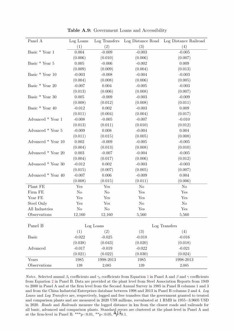
Table A.9: Government Loans and Accessibility

Panel A Log Loans Log Transfers Log Distance Road Log Distance Railroad(1) (2) (3) (4)

Basic * Year 1 0.004 -0.009 -0.003 -0.005(0.006) (0.010) (0.006) (0.007)

Basic * Year 5 0.005 -0.006 -0.002 0.009(0.009) (0.009) (0.004) (0.013)

Basic * Year 10 -0.003 -0.008 -0.004 -0.003(0.004) (0.008) (0.006) (0.005)

Basic * Year 20 -0.007 0.004 -0.005 -0.003(0.013) (0.006) (0.008) (0.007)

Basic * Year 30 0.005 -0.009 -0.003 -0.009(0.008) (0.012) (0.008) (0.011)

Basic * Year 40 -0.012 0.002 -0.003 0.009(0.011) (0.004) (0.004) (0.017)

Advanced * Year 1 -0.008 -0.005 -0.007 -0.010(0.013) (0.011) (0.010) (0.012)

Advanced * Year 5 -0.009 0.008 -0.004 0.004(0.011) (0.015) (0.005) (0.008)

Advanced * Year 10 0.002 -0.009 -0.005 -0.005(0.004) (0.013) (0.008) (0.010)

Advanced * Year 20 0.003 -0.007 -0.004 -0.005(0.004) (0.017) (0.006) (0.012)

Advanced * Year 30 -0.012 0.002 -0.003 -0.003(0.015) (0.007) (0.005) (0.007)

Advanced * Year 40 -0.007 0.006 -0.009 0.004(0.008) (0.015) (0.011) (0.006)

Plant FE Yes Yes No NoFirm FE No No Yes YesYear FE Yes Yes Yes YesSteel Only Yes Yes No NoAll Industries No No Yes YesObservations 12,160 12,160 5,560 5,560

Panel B Log Loans Log Transfers(1) (2) (3) (4)

Basic -0.022 -0.025 -0.018 -0.016(0.038) (0.043) (0.020) (0.018)

Advanced -0.017 -0.019 -0.022 -0.021(0.021) (0.022) (0.030) (0.024)

Years 1985 1998-2013 1985 1998-2013Observations 139 2,085 139 2,085

Notes. Selected annual �t coefficients and �t coefficients from Equation 1 in Panel A and � and � coefficientsfrom Equation 2 in Panel B. Data are provided at the plant level from Steel Association Reports from 1949to 2000 in Panel A and at the firm level from the Second Annual Survey in 1985 in Panel B columns 1 and 3and from the China Industrial Enterprises database between 1998 and 2013 in Panel B columns 2 and 4. LogLoans and Log Transfers are, respectively, logged and free transfers that the government granted to treatedand comparison plants and are measured in 2020 US$ millions, reevaluated at 1 RMB in 1955=3.9605 USDin 2020. Roads and Railroads measure the logged distance in km from the closest roads and railroads forall basic, advanced and comparison plants. Standard errors are clustered at the plant-level in Panel A andat the firm-level in Panel B. ***p<0.01, **p<0.05, *p<0.1.A14

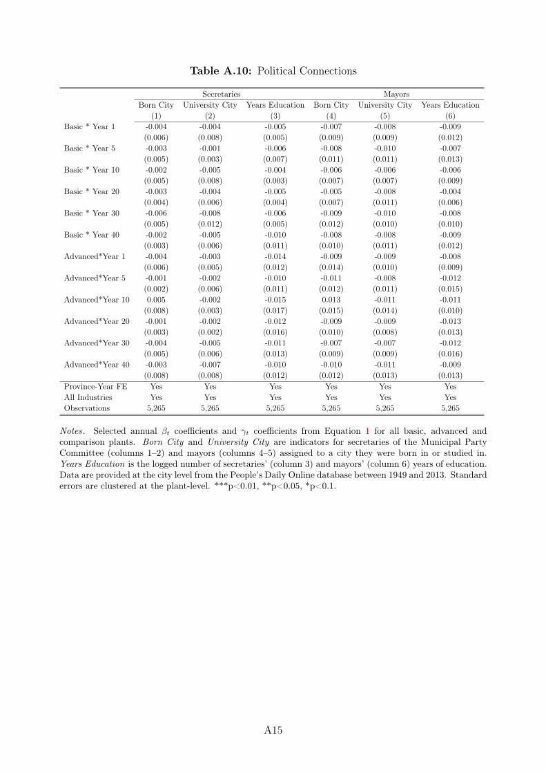
Table A.10: Political Connections

Secretaries MayorsBorn City University City Years Education Born City University City Years Education

(1) (2) (3) (4) (5) (6)Basic * Year 1 -0.004 -0.004 -0.005 -0.007 -0.008 -0.009

(0.006) (0.008) (0.005) (0.009) (0.009) (0.012)Basic * Year 5 -0.003 -0.001 -0.006 -0.008 -0.010 -0.007

(0.005) (0.003) (0.007) (0.011) (0.011) (0.013)Basic * Year 10 -0.002 -0.005 -0.004 -0.006 -0.006 -0.006

(0.005) (0.008) (0.003) (0.007) (0.007) (0.009)Basic * Year 20 -0.003 -0.004 -0.005 -0.005 -0.008 -0.004

(0.004) (0.006) (0.004) (0.007) (0.011) (0.006)Basic * Year 30 -0.006 -0.008 -0.006 -0.009 -0.010 -0.008

(0.005) (0.012) (0.005) (0.012) (0.010) (0.010)Basic * Year 40 -0.002 -0.005 -0.010 -0.008 -0.008 -0.009

(0.003) (0.006) (0.011) (0.010) (0.011) (0.012)Advanced*Year 1 -0.004 -0.003 -0.014 -0.009 -0.009 -0.008

(0.006) (0.005) (0.012) (0.014) (0.010) (0.009)Advanced*Year 5 -0.001 -0.002 -0.010 -0.011 -0.008 -0.012

(0.002) (0.006) (0.011) (0.012) (0.011) (0.015)Advanced*Year 10 0.005 -0.002 -0.015 0.013 -0.011 -0.011

(0.008) (0.003) (0.017) (0.015) (0.014) (0.010)Advanced*Year 20 -0.001 -0.002 -0.012 -0.009 -0.009 -0.013

(0.003) (0.002) (0.016) (0.010) (0.008) (0.013)Advanced*Year 30 -0.004 -0.005 -0.011 -0.007 -0.007 -0.012

(0.005) (0.006) (0.013) (0.009) (0.009) (0.016)Advanced*Year 40 -0.003 -0.007 -0.010 -0.010 -0.011 -0.009

(0.008) (0.008) (0.012) (0.012) (0.013) (0.013)Province-Year FE Yes Yes Yes Yes Yes YesAll Industries Yes Yes Yes Yes Yes YesObservations 5,265 5,265 5,265 5,265 5,265 5,265

Notes. Selected annual �t coefficients and �t coefficients from Equation 1 for all basic, advanced andcomparison plants. Born City and University City are indicators for secretaries of the Municipal PartyCommittee (columns 1–2) and mayors (columns 4–5) assigned to a city they were born in or studied in.Years Education is the logged number of secretaries’ (column 3) and mayors’ (column 6) years of education.Data are provided at the city level from the People’s Daily Online database between 1949 and 2013. Standarderrors are clustered at the plant-level. ***p<0.01, **p<0.05, *p<0.1.

A15

Table A.11: County-Level Government Investments

Log Investment Log Other Projects Log InfrastructureAll Related Industries Unrelated Industries(1) (2) (3) (4) (5)

Basic * Post -0.019 -0.011 0.015 -0.014 0.021(0.025) (0.044) (0.028) (0.015) (0.038)

Advanced * Post -0.022 0.009 -0.005 0.012 0.014(0.023) (0.003) (0.010) (0.011) (0.020)

County-Year FE Yes Yes Yes Yes YesObservations 3,240 3,240 3,240 3,240 3,240

Notes. Basic is an indicator equal to one for counties where plants that received a basic transfer werelocated. Advanced is an indicator equal to one for counties where plants that received an advanced transferwere located. Post Log Investment is logged government investment in all industries, in industries relatedto the 156 Projects and in unrelated industries. Log Other Projects is logged number of industrial projectsfinanced by the Chinese government to promote industrialization after the end of the Sino-Soviet Alliance.Log Infrastructure is logged government investment in infrastructure. Data are provided at the county levelfrom the Statistical Yearbooks between 1949 and 2008. Standard errors are clustered at the county level.***p<0.01, **p<0.05, *p<0.1.

Table A.12: Correlation between Comparison Plants and Other Steel Plants

Log Output Log TFPQ Log Workersaaaaaaaaaaaaaaaaaaaaaaaaaaaaaaaaaaaaaaaaaaaa (1) (2) (3)Comparison * Year 1 0.022 0.011 0.010

(0.015) (0.010) (0.008)Comparison* Year 5 0.029*** 0.012*** 0.015***

(0.010) (0.004) (0.005)Comparison* Year 10 0.033*** 0.014*** 0.020***

(0.011) (0.005) (0.006)Comparison* Year 20 0.035*** 0.015*** 0.022***

(0.007) (0.005) (0.007)Comparison* Year 30 0.039*** 0.014*** 0.023***

(0.010) (0.004) (0.006)Comparison* Year 40 0.035*** 0.010*** 0.020***

(0.007) (0.003) (0.005)Plant FE Yes Yes YesYear FE Yes Yes YesObservations 36,220 36,220 36,220

Notes. The sample includes comparison plants and steel plants built by the Chinese government underindustrial projects started after the Sino-Soviet Split. Comparison is an indicator for plants built as partof the 156 Projects. Log Output is logged quantities (in tons) of steel. Log TFPQ is logged total factorproductivity quantity, computed as log TFPQ = log TFPR � p̃, where ep is the revenue share weightedaverage of the prices of plant products and TFPR is calculated using Gandhi et al. (2020)’s method. LogWorkers is logged number of workers. Data are provided at the plant level from the Steel AssociationReports between 1949 and 2000. Standard errors are clustered at the plant-level. *** p < 0.01, ** p < 0.05,* p < 0.1.

A16

Table A.13: Bounding Based on Correlation Between Observables and Unobservables

Main Results � = 0.1 � = 0.2 � = 0.4 � = 0.6 � = 0.8 � = 1 � for � = 0(1) (2) (3) (4) (5) (6) (7) (8)

Panel A: OutputBasic * Year 1 0.002 0.002 0.002 0.003 0.002 0.002 0.002Basic * Year 5 0.113 0.109 0.108 0.105 0.103 0.101 0.099 8.34Basic * Year 10 0.130 0.124 0.122 0.121 0.120 0.118 0.117 9.32Basic * Year 20 0.085 0.083 0.081 0.079 0.077 0.074 0.073 9.87Basic * Year 30 0.039 0.036 0.033 0.029 0.026 0.024 0.021Basic * Year 40 0.009 0.008 0.007 0.006 0.007 0.005 0.007Advanced * Year 1 0.062 0.057 0.055 0.053 0.051 0.049 0.046 10.98Advanced * Year 5 0.089 0.087 0.085 0.082 0.079 0.075 0.071 11.77Advanced * Year 10 0.098 0.095 0.093 0.090 0.082 0.080 0.077 12.54Advanced * Year 20 0.180 0.177 0.173 0.171 0.169 0.167 0.163 14.61Advanced * Year 30 0.292 0.288 0.285 0.283 0.278 0.276 0.270 16.87Advanced * Year 40 0.402 0.398 0.395 0.392 0.390 0.387 0.381 19.12

Panel B: TFPQBasic * Year 1 0.001 0.001 0.001 0.002 0.001 0.001 0.001Basic * Year 5 0.108 0.105 0.102 0.100 0.098 0.095 0.091 8.01Basic * Year 10 0.128 0.122 0.120 0.119 0.1150 0.111 0.108 8.93Basic * Year 20 0.081 0.080 0.077 0.075 0.071 0.070 0.069 9.57Basic * Year 30 0.035 0.033 0.031 0.025 0.023 0.021 0.018Basic * Year 40 0.002 0.002 0.002 0.002 0.002 0.002 0.01Advanced * Year 1 0.061 0.055 0.051 0.048 0.046 0.044 0.041 12.17Advanced * Year 5 0.078 0.073 0.069 0.065 0.063 0.061 0.059 12.67Advanced * Year 10 0.093 0.092 0.089 0.087 0.081 0.079 0.072 14.91Advanced * Year 20 0.173 0.170 0.166 0.162 0.160 0.158 0.155 15.32Advanced * Year 30 0.281 0.278 0.273 0.270 0.267 0.262 0.2590 17.34Advanced * Year 40 0.391 0.387 0.384 0.381 0.378 0.373 0.371 19.06

Notes. The table shows how different hypotheses on the degree of correlation between observables andunobservables affect selected �t and �t coefficients from Equation 1. The notation follows Oster (2019).The coefficient � is the relative degree of selection on observed and unobserved variables. Rmax is thehypothetical R squared in a regression that includes both observables and unobservables. R̃ is the R squaredin the regression that includes only observables (Figure 3). Oster (2019) finds that Rmax = 1.3 and � = 1are appropriate bounds to calculate bias-adjusted treatment effects. Output is logged quantities (in milliontons) of steel. TFPQ is logged total factor productivity quantity, computed as log TFPQ = log TFPR� p̃,where ep is the revenue share weighted average of the prices of plant products and TFPR is calculated usingthe Gandhi et al. (2020)’s method.

A17

Table A.14: Bounding Based on Correlation Between Observables and Unobservables

Main Results � = 1Rmax = 1.10R̃ Rmax = 1.20R̃ Rmax = 1.30R̃ Rmax = 1.40R̃ Rmax = 1.50R̃ Rmax = 2R̃

(1) (2) (3) (4) (5) (6) (7)Panel A: OutputBasic * Year 1 0.002 0.002 0.002 0.003 0.002 0.002 0.002Basic * Year 5 0.113 0.110 0.107 0.104 0.102 0.100 0.096Basic * Year 10 0.130 0.128 0.125 0.120 0.117 0.113 0.111Basic * Year 20 0.085 0.082 0.080 0.077 0.075 0.073 0.070Basic * Year 30 0.039 0.035 0.031 0.028 0.024 0.020 0.018Basic * Year 40 0.009 0.007 0.006 0.006 0.006 0.005 0.003Advanced * Year 1 0.062 0.055 0.053 0.050 0.049 0.047 0.041Advanced * Year 5 0.089 0.085 0.081 0.080 0.074 0.073 0.070Advanced * Year 10 0.098 0.095 0.090 0.088 0.085 0.081 0.079Advanced * Year 20 0.180 0.176 0.172 0.168 0.167 0.166 0.162Advanced * Year 30 0.292 0.285 0.283 0.281 0.277 0.274 0.271Advanced * Year 40 0.402 0.397 0.394 0.390 0.387 0.385 0.379

Panel B: TFPQBasic * Year 1 0.001 0.001 0.001 0.002 0.001 0.002 0.002Basic * Year 5 0.108 0.106 0.103 0.100 0.099 0.096 0.093Basic * Year 10 0.128 0.124 0.121 0.118 0.114 0.111 0.099Basic * Year 20 0.081 0.080 0.078 0.074 0.071 0.070 0.068Basic * Year 30 0.035 0.032 0.029 0.024 0.020 0.019 0.014Basic * Year 40 0.002 0.002 0.003 0.003 0.002 0.002 0.002Advanced * Year 1 0.061 0.055 0.053 0.050 0.049 0.047 0.041Advanced * Year 5 0.078 0.073 0.070 0.069 0.068 0.065 0.061Advanced * Year 10 0.093 0.090 0.088 0.084 0.080 0.079 0.078Advanced * Year 20 0.173 0.173 0.170 0.165 0.161 0.159 0.155Advanced * Year 30 0.281 0.285 0.283 0.281 0.277 0.274 0.271Advanced * Year 40 0.391 0.388 0.383 0.380 0.378 0.374 0.369

Notes. The table shows how different hypotheses on Rmax affect selected �t and �t coefficients from Equation1.. The notation follows Oster (2019). The coefficient � is the relative degree of selection on observed andunobserved variables. Rmax is the hypothetical R squared in a regression that includes both observablesand unobservables. R̃ is the R squared in the regression that includes only observables (Figure 3). Oster(2019) finds that Rmax = 1.3 and � = 1 are appropriate bounds to calculate bias-adjusted treatment effects.Output is logged quantities (in million tons) of steel. TFPQ is logged total factor productivity quantity,computed as log TFPQ = log TFPR � p̃, where ep is the revenue share weighted average of the prices ofplant products and TFPR is calculated using the Gandhi et al. (2020)’s method.

A18

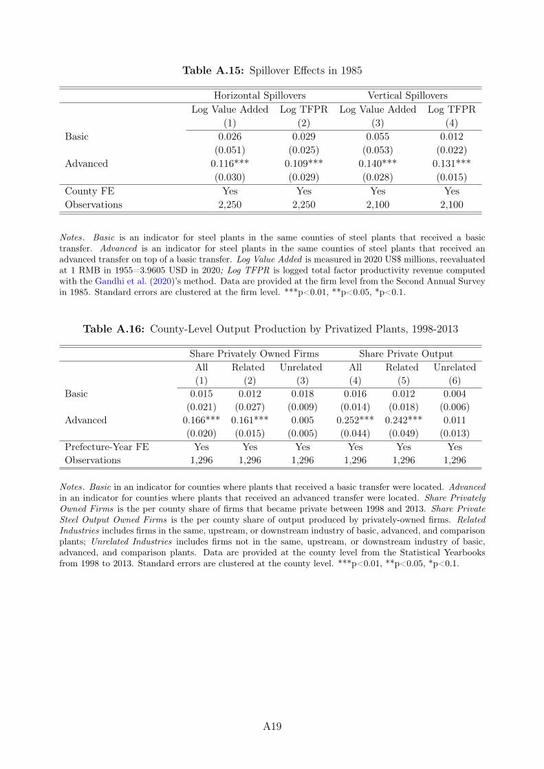
Table A.15: Spillover Effects in 1985

Horizontal Spillovers Vertical SpilloversLog Value Added Log TFPR Log Value Added Log TFPR

aaaaaaaaaaaaaaaaaaaaa (1) (2) (3) (4)Basic 0.026 0.029 0.055 0.012

(0.051) (0.025) (0.053) (0.022)Advanced 0.116*** 0.109*** 0.140*** 0.131***

(0.030) (0.029) (0.028) (0.015)County FE Yes Yes Yes YesObservations 2,250 2,250 2,100 2,100

Notes. Basic is an indicator for steel plants in the same counties of steel plants that received a basictransfer. Advanced is an indicator for steel plants in the same counties of steel plants that received anadvanced transfer on top of a basic transfer. Log Value Added is measured in 2020 US$ millions, reevaluatedat 1 RMB in 1955=3.9605 USD in 2020; Log TFPR is logged total factor productivity revenue computedwith the Gandhi et al. (2020)’s method. Data are provided at the firm level from the Second Annual Surveyin 1985. Standard errors are clustered at the firm level. ***p<0.01, **p<0.05, *p<0.1.

Table A.16: County-Level Output Production by Privatized Plants, 1998-2013

Share Privately Owned Firms Share Private Outputaaaaaaaaaaaaaaaaaaaa All Related Unrelated All Related Unrelated

(1) (2) (3) (4) (5) (6)Basic 0.015 0.012 0.018 0.016 0.012 0.004

(0.021) (0.027) (0.009) (0.014) (0.018) (0.006)Advanced 0.166*** 0.161*** 0.005 0.252*** 0.242*** 0.011

(0.020) (0.015) (0.005) (0.044) (0.049) (0.013)Prefecture-Year FE Yes Yes Yes Yes Yes YesObservations 1,296 1,296 1,296 1,296 1,296 1,296

Notes. Basic in an indicator for counties where plants that received a basic transfer were located. Advancedin an indicator for counties where plants that received an advanced transfer were located. Share PrivatelyOwned Firms is the per county share of firms that became private between 1998 and 2013. Share PrivateSteel Output Owned Firms is the per county share of output produced by privately-owned firms. RelatedIndustries includes firms in the same, upstream, or downstream industry of basic, advanced, and comparisonplants; Unrelated Industries includes firms not in the same, upstream, or downstream industry of basic,advanced, and comparison plants. Data are provided at the county level from the Statistical Yearbooksfrom 1998 to 2013. Standard errors are clustered at the county level. ***p<0.01, **p<0.05, *p<0.1.

A19

Table A.17: Channels of Persistence of the Soviet Technology Transfer

STEM Universities Technical Schools College Graduates High-Skilled Workersaaaaaaaaaaaaaaaaaaa (1) (2) (3) (4)Basic 0.009 -0.010 0.015 0.007

(0.013) (0.012) (0.021) (0.011)Advanced 0.104*** 0.156*** 0.133*** 0.162***

(0.034) (0.041) (0.030) (0.035)Prefecture-Year FE Yes Yes Yes YesObservations 1,296 1,296 1,296 1,296

Notes. Basic in an indicator for counties where plants that received a basic transfer were located. Advancedin an indicator for counties where plants that received an advanced transfer were located. STEM Universitiesis the share of universities offering a STEM degree per county. Technical schools is the number of technicalschools per inhabitant county. College Graduates and High-Skilled Workers are the logged number of collegegraduates and high-skilled technicians over population per county. Data are provided at the county levelfrom the China Education Yearbooks from 1998 to 2013. Standard errors are clustered at the county-level.***p<0.01, **p<0.05, *p<0.1.

A20

Table A.18: Aggregate Effects of the Soviet Technology Transfer

Panel A: Province-Level Outcomes

Log Ind. Output Log Ind. Employment Log GDP Capita(1) (2) (3)

Share Basic Projects * Post 1952 0.431*** 0.132*** 0.297***(0.115) (0.035) (0.081)

Share Advanced Projects * Post 1952 1.065*** 0.328*** 1.309***(0.278) (0.066) (0.311)

Observations 963 963 963Province FE Yes Yes YesYear FE Yes Yes Yes

Panel B: Cross-Sectional Multiplier

�GDP capitaMedium Term (1953–1978) Long Term (1953-–2008)

(1) (2) (4) (5)Basic Projects Capita 0.251*** 0.255*** 0.169*** 0.173***

(0.021) (0.024) (0.027) (0.031)Advanced Projects Capita 0.583*** 0.589*** 0.201*** 0.209***

(0.039) (0.041) (0.043) (0.042)Observations 963 963 963 963Province FE Yes Yes Yes YesLinear Trend No Yes No YesYear FE Yes Yes Yes Yes

Notes. Share Basic Projects is the share of basic projects out of all projects contemplated in a givenprovince. Share Advanced Projects is the share of advanced projects out of all projects contemplated ina given province. Post 1952 is an indicator equal to one for years after 1952. Log Ind. Output, Ind.Employment, GDP Capita, are the province-level logged industrial output, industrial employment, andGDP per capita. Basic Projects per Capita is the province investment in basic projects over population in1949; Advanced Projects per Capita is the province investment in advanced projects over population in 1949;�GDP per Capitapt is the variation in GDP per capita in province p between year t and year t-1 with t2 [1949, 2008]. Data are provided at the province level from the Statistical Yearbooks between 1949 and2008. Standard errors are wild-bootstrapped at the province level with 1,000 replications (Cameron et al.,2008). ***p<0.01, **p<0.05, *p<0.1.

A21

B Data Collection and Dataset Construction

In this Appendix, we provide a detailed description of our primary data sources and howwe constructed the dataset, as well as a list of all the variables we use in the paper,with their definitions, aggregation level, time period, and sources (Appendix Table B.2).When needed, we also provide additional details on the variables’ construction.

B.1 Description of Primary Sources

Our data collection targeted the 156 Projects approved under the Sino-Soviet Alliancebetween 1950 and 1957. To retrieve the list of such projects, we relied on the officialsigned agreements between the Soviet Union and China from the National Archives Ad-ministration of China, whose access is restricted and was occasionally granted for thispaper. For each project, we collected and digitized detailed information on the projectname and location, the name of the plant built, industry, size and capacity, number ofworkers, and whether it was completed with Soviet assistance or by China only due to theSino-Soviet split. To make sure we collected the official agreements for all the approvedprojects, we also gathered data from the Selected Archival Materials on the PRC’s Econ-

omy, a collection of documents on the PRC’s economic development between 1949 and1957, that includes detailed summaries of the 156 Projects. A comparison of these sum-maries with the official agreements reveals that the former contain no additional projectsor project information beyond that found in the latter. We also compared our digitizedlist of projects against two historical studies in Chinese on the Sino-Soviet technologytransfer program that independently collected the 156 technology transfer projects fromthe National Archives Administration of China as well (Zhang et al., 2003; Dong and Wu,2004). Specifically, we checked for any differences or additional information on projectname, start and completion years, and location, as well as project industry, size, andcapacity. Neither Zhang et al. (2003) nor Dong and Wu (2004) provide any additional ordifferent project information, for any of the projects, beyond that contained in our data.

We then constructed a panel dataset of plant performance and county/province out-comes, gathering data from four different sources.

Steel Association Reports (1949–2000). These reports, compiled yearly from1949 to 2000, contain restricted data on all 94 Chinese firms in the steel industry for atotal of 1,410 plants. They contain detailed information on plant quantity and type ofsteel products, input utilization, the specific machinery in use, capital, fixed investment,profits, and number and types of workers (unskilled workers, high-skilled workers, andengineers), all of which we manually collected and digitized in different rounds between

B1

August 2020 and December 2021.Second Industrial Survey (1985). In the early 1980s, the Chinese government be-

gan implementing several reforms on market liberalization. Until then, stretching backto the RPC’s founding in 1949, there had been a lack of systematic data on firm andindustry structure. This survey, conducted by Statistics China in 1985, was therefore un-dertaken for policy makers to learn about the structure of the industries and enterprises,the products, the state of technology and equipment, the economic value of enterprises,and the quality of their workforce. This information constituted a guide for subsequentpolicies and reforms. As such, the survey covered more than 40 industries within the sec-ondary sector. It is considered the most comprehensive dataset on industrial enterprisesfrom the founding of the PRC through to the early 1990s.1 The firm-level-data portionof the survey, though still confidential today, has been declassified for this project; itcovers the 7,592 largest firms operating in China in 1985.2 For each of them, the Surveygathered data on output, sales, profits, fixed assets, raw materials, total wages, num-ber of employees, finished product inventory, main products, production equipment, andyear of establishment, which we manually collected and digitized. We have also manuallycollected and digitized the county-level and prefecture-level industrial production datareported in the survey (which is stored internally at Statistics China, in Beijing).

China Industrial Enterprises Database (1998–2013). This database, compiledby Statistics China yearly between 1998 and 2013 to compute GDP, covers more than1 million publicly listed and private industrial enterprises whose asset value exceeded 5million yuan prior to 2011, and 20 million yuan after 2011. All industrial firms in thedatabase are required to file an annual report of their production activities, as well astheir accounting and financial information. Statistics China implemented strict double-checking standards for verifying the accuracy of firm-reported information. For each firm,the database contains data on output, number of employees, profits, ownership structure,and capital investment.

Statistical Yearbook of China (1949–2000). We manually collected and digitizedprovince-level data from all the published statistical yearbooks compiled by StatisticsChina between 1949 and 2000. This dataset contains province-level information on GDP,1 The First Industrial Survey was conducted in 1950, right after the PRC was founded. Its goal wasestimating the “lay of the land” regarding the national industrial and mining enterprises, a basis for therecovery from the Civil War and subsequent development. However, this survey contains no firm-leveldata, and it predates the construction of treated and comparison plants. For this reason, we cannotemploy it in our paper.

2 The Second Industrial Survey reported that in 1985 there were 437,200 firms operating in China andthat it collected firm-level data for the 7,592 largest ones, but the official guidelines of the survey donot provide a formal size threshold for inclusion in the survey itself. We computed that the surveyedcompanies comprised only 1.74% of total Chinese firms but produced 62.46% of the industrial outputin 1985.

B2

population, capital, investment, and number of workers.Data Validation. While dealing with plant-level data, one always has to consider the

possibility that the outcomes provided by the plants may not be accurate. In our context,for instance, plant supervisors may have misreported their production information to showbetter-than-actual performance. Two important institutional details matter here. First,our main data source, the Steel Association Reports, was highly monitored and checkedby industry peers, which strongly limited the possibility of manipulation. Moreover,the officially-released aggregate production data was complied by Statistics China, adifferent and independent source. Manipulations were therefore more likely to occur in thelatter rather than in the former reports. Second, after the Sino-Soviet Split, the Chinesegovernment wanted to tie up loose ends with the Soviet Union as quickly as possible. Assuch, data manipulation should have aimed at lowering the performance of Soviet-treatedplants, which would go against us finding a positive effect of the Soviet transfer. This isespecially true during the Great Leap Forward, when the Chinese government wanted toshow the efficacy of labor-intensive methods of industrialization, which would emphasizemanpower rather than machines and capital expenditure, in stark contrast with the goalsof the Soviet transfer (Clark, 1973; Lardy, 1995).

Beyond these consideration, we cross-checked our data against different sources, asfollows. First, we turned to Clark (1995) who studied the Chinese steel industry, bycollecting data on steel plants with a capacity of at least 100,000 tons, between 1949 and1993. Specifically, for each plant, he estimated the minimum and the maximum yearlysteel output based on the capital in use, concluding that the data from the Steel Associa-tion annual reports, our main source, appear credible. We repeat our main analysis usingClark (1995)’s data and find that our estimated coefficients using the annual reports arebetween the coefficients obtained using their minimum and maximum estimates (TableB.1, columns 2, 3, 6 and 7).3 Even assuming that basic and advanced plants produced atthe minimum and comparison plants at the maximum level estimated by Clark (1995),we would still find a persistent effect of the advanced transfer and a short-lived effect ofthe basic transfer, in line with our main results (Table B.1, columns 4-8).

Second, for the Ansteel Company in Anshan, we were able to collect the plant’s ownproduction data, which it stored in its historical records (Ji, 2019). These data wereintended for internal use and were not shared with the central government. When wecompared this data with the data from the Steel Association Reports, we found that theyare remarkably similar, with a correlation of 0.981.

Third, we summarized the industrial output of firms in the Second Industrial Survey by3 As Clark (1995)’s study goes until 1993, we can repeat our main analysis only in the first 30 yearsafter the Soviet transfer.

B3

counties and prefectures, comparing this data with the county-level and prefecture-levelindustrial output data reported in the survey. The two sets of data are also remarkablysimilar, with a correlation of 0.989.

Fourth, we summarized the industrial output of firms in the Second Industrial Surveyby provinces, comparing it with total province-level industrial output from the StatisticalYearbook of China in 1985. The two sets of data are comparable, with a correlation of0.974.

Data Digitization. Between August 2019 and December 2021, we employed four re-search assistants (undergraduate students at Tsinghua University and Peking University)to digitize the newly collected data. On top of manually performing the data entry, theresearch assistants were asked to cross-check their work to ensure that all the data werecorrectly digitized. Bo Li also personally checked the accuracy of 75% of the data entries.

B.2 Matching Across Different Data Sources

To match the plants built in the 156 Projects with their outcomes across different sources,we proceeded as follows. For plants in the steel industry, we used plant name, location,county, and province; we manually and uniquely matched all 304 steel plants eligible toparticipate in the technology transfer program with their annual reports. For plants in allindustries, we used firm name, location, county, and province; we manually and uniquelymatched all 139 firms eligible to participate in the technology transfer program with theiroutcomes in 1985 and between 1998 and 2013.

B.3 Geolocalization of Basic, Advanced and Comparison Plants

The Second Industrial Survey records each firm’s address in 1984. To geolocalize the firms,we searched the 1984 address of each firm on Gaode Map, an online GPS browser thatprovides a high-quality map of China. If we could find the 1984 address in Gaode Map, weuse Gaode Map’s geocoding API to transfer the 1984 address to the geographic location,based on latitude and longitude. For 3,426 of the 7,592 firms covered by the SecondIndustrial Survey (45%), their 1984 addresses cannot be found, because the name ofstreets, villages, or towns changed. We therefore manually searched these 1984 addresseson the websites of local governments that keep track of name changes and found howthe addresses changed from 1984 and the corresponding current addresses. In this way,we were able to obtain the geographic locations of all the firms based on the currentaddresses.4

4 From 1990 to 2013, Chinese prefecture cities were subject to some jurisdictional changes. However,because we retrieve firm latitude and longitude, these changes do not affect firm geolocalization.

B4

Between 1998 and 2013, the China Industrial Enterprises database records the firmname only. We searched firms by their name in Tianyancha, a comprehensive databaseon all registered Chinese firms, which provides the firms’ current address. We obtainedall firms’ addresses and used Gaode Map’s geocoding API to transfer the addresses togeographic locations, based on latitudes and longitudes.

B.4 Identification of Firms Economically Related to Basic, Ad-

vanced and Comparison Plants

We constructed a list of firms economically related to basic, advanced and comparisonplants as follows. We retrieved each firm’s two-digit industry code from the Steel Associ-ation Reports or the Second Industrial Survey, from which we observe the firm products.If firms had the same two-digit industry code of basic, advanced and comparison plants,we consider them operating in the same industry and include them in the horizontalspillover analysis. If firms had a different two-digit industry, we use the input-outputtables of the closest available year to assess whether firm products were upstream ordownstream, relative to the products of the treated and comparison plants. If productswere neither upstream nor downstream, we consider firms not economically related tobasic, advanced and comparison plants. After the National Bureau of Statistics of China(NBS) began compiling its Input-Output Tables in 1987, every five years (in the yearsending with 2 and 7) it conducts the national input-output survey and compiles thebenchmark input-output tables of the corresponding year. We therefore used the 1987Input-Output Tables (for the Second Industrial Survey data of 1985) and the 1997, 2002,2007, and 2012 Input-Output Tables (for the China Industrial Enterprises database of1998–2013).

B5

Table B.1: Robustness Checks using Alternative Data Sources

Log Output (1–5) Log TFPQ (6–10)

(1) (2) (3) (4) (5) (6) (7) (8)

Basic * Year 1 0.002 0.001 0.003 0.001 0.001 0.002 0.001 0.003

(0.018) (0.016) (0.015) (0.016) (0.017) (0.013) (0.011) (0.015)

Basic * Year 5 0.113*** 0.179*** 0.101*** 0.077*** 0.106*** 0.173*** 0.096*** 0.068***

(0.017) (0.020) (0.015) (0.015) (0.018) (0.021) (0.012) (0.015)

Basic * Year 10 0.130*** 0.203*** 0.117*** 0.085*** 0.128*** 0.189*** 0.189*** 0.076***

(0.025) (0.028) (0.019) (0.022) (0.023) (0.022) (0.020) (0.018)

Basic * Year 20 0.085* 0.095* 0.079* 0.055* 0.081* 0.088* 0.073* 0.046*

(0.046) (0.052) (0.045) (0.034) (0.047) (0.050) (0.048) (0.027)

Basic * Year 30 0.039 0.045 0.033 0.021 0.035 0.041 0.027 0.019

(0.044) (0.049) (0.041) (0.033) (0.041) (0.043) (0.031) (0.033)

Advanced * Year 1 0.062*** 0.081*** 0.055*** 0.050*** 0.061*** 0.073*** 0.050*** 0.043***

(0.017) (0.023) (0.016) (0.015) (0.016) (0.018) (0.015) (0.012)

Advanced * Year 5 0.089*** 0.101*** 0.078*** 0.066*** 0.078*** 0.097*** 0.069*** 0.057***

(0.018) (0.027) (0.016) (0.013) (0.018) (0.019) (0.019) (0.015)

Advanced * Year 10 0.098*** 0.155*** 0.086*** 0.079*** 0.093*** 0.143*** 0.077*** 0.066***

(0.029) (0.033) (0.026) (0.02) (0.026) (0.029) (0.025) (0.020)

Advanced * Year 20 0.180*** 0.267*** 0.167*** 0.154*** 0.173*** 0.253*** 0.156*** 0.142***

(0.030) (0.044) (0.036) (0.027) (0.029) (0.029) (0.028) (0.018)

Advanced * Year 30 0.292*** 0.309*** 0.283*** 0.272*** 0.281*** 0.289*** 0.271*** 0.261***

(0.038) (0.041) (0.031) (0.026) (0.037) (0.031) (0.037) (0.034)

Specification Main Max Min Min-Max Main Max Min Min-Max

Observations 12,160 12,160 12,160 12,160 12,160 12,160 12,160 12,160

Notes. Selected annual �t coefficients and �t coefficients from Equation 1 (columns 1 and 5), usingthe minimum production estimates from Clark (1995) (columns 2 and 6), the maximum productionestimates (columns 3 and 7), and the minimum production estimates for basic and advanced plantsand the maximum production estimates for comparison plants (columns 4 and 8). Output is loggedquantities (in million tons) of steel. TFPQ is logged total factor productivity quantity, computed aslog TFPQ = log TFPR�p̃, where ep is the revenue-share weighted average of the prices of plant products,and TFPR is calculated using Gandhi et al. (2020)’s method. Standard errors are clustered at the plantlevel. *** p < 0.01, ** p < 0.05, * p < 0.1.

B6

Table B.2: List of Variables, With Their Definitions and Sources

Variable Definition Level, Source and Years of Coverage

Log Steel Logged million tons of steel produced Plant-year, Steel Association, 1949–2000

Log Coke/Iron/Pig Iron Logged million tons of coke/ iron/ pig iron used as input Plant-year, Steel Association, 1949–2000

Log TFPQ Total Factor Productivity Quantity; for estimation, see Appendix C. Plant-year, Steel Association, 1949–2000

Log Oxygen Logged tons of steel produced with the basic oxygen process Plant-year, Steel Association, 1949–2000

Log Continuous Casting Logged tons of steel produced with the continuous casting method Plant-year, Steel Association, 1985–2000

Log International Standard Logged million tons of steel above international standard Plant-year, Steel Association, 1985–2000

% Engineers Share of engineers out of total employment Plant-year, Steel Association, 1949–2000

% Technicians Share of high-skilled technicians out of total employment Plant-year, Steel Association, 1949–2000

% Unskilled Share of unskilled workers out of total employment Plant-year, Steel Association, 1949–2000

Log Workers Total number of workers Plant-year, Steel Association, 1949–2000

Log Value Added Difference between firm gross income and intermediate inputs Firm-year, Second Industrial Survey, 1985; China Industrial Enterprises, 1998–2013

Log Fixed Assets Logged value of land, buildings, and machines owned by the firm Plant-year, Steel Association, 1949–2000

Firm-year, Second Industrial Survey, 1985; China Industrial Enterprises, 1998–2013

Log Capital Stock Calculated from gross fixed assets using the Perpetual Inventory Method (PIM), Plant-year, Steel Association, 1949–2000

see table notes. Firm-year, Second Industrial Survey, 1985; China Industrial Enterprises, 1998–2013

Log TFPR Total Factor Productivity Revenue; for estimation see Appendix C. Firm-year, Second Industrial Survey, 1985; China Industrial Enterprises, 1998–2013

Log Revenues Operating revenues Firm-year, Second Industrial Survey, 1985; China Industrial Enterprises, 1998–2013

Log Exports Logged value of exports Firm-year, China Industrial Enterprises, 1998–2013

Log Industrial Output Logged value of industrial production Province-year, Statistical Yearbook, 1949–2013

Log Industrial Employment Logged number of workers in industrial sector Province-year, Statistical Yearbook, 1949–2013

Log GDP Capita Logged GDP per capita Province-year, Statistical Yearbook, 1949-–2013

Log Investment Logged value of government investments Province-year, Statistical Yearbook, 1949–2013

STEM Universities Share of universities offering a STEM degree per county County-year, China Education Yearbooks, 1998-–2013

Technical School Number of technical schools per inhabitant per county County-year, China Education Yearbooks, 1998-–2013

Log College Graduates Logged number of college graduates over population County-year, China Education Yearbooks, 1998-–2013

Log High-Skilled Workers Logged number of high-skilled workers over population County-year, China Education Yearbooks, 1998-–2013Notes. To obtain a measure of firm capital stock from the fixed gross assets (fga), we use the Perpetual Inventory Method (PIM). First, we compute investment I as the difference betweenthe deflated current and the lagged fga, and use the PIM formula Pt+1Kt+1 = Pt+1(1� �)PtKt + Pt+1It+1, where K is the quantity of capital, P is its price (set equal to one percent, theinterest rate to be paid back to the Soviet Union for the loan granted to China for the technology transfer program), I is investment, and � is the depreciation rate (set equal to 3.5 percent,according to the average estimated life of machine of 20 years (Lardy, 1995). However, this procedure is valid only if the base-year capital stock (the first year in the data for a given firm)can be written as P0K0 , which is not the case here because fga is reported at its historic cost. To estimate its value at replacement cost, we use the RG factor suggested by Balakrishnan etal. (2000), RG = [(1+g)⌧+1�1](1+⇡)⌧ [(1+g)(1+⇡)�1]

g{[(1+g)(1+⇡)]⌧+1�1} , where ⌧ is the average life of machines (assumed to be 20 years, according to Lardy, 1995), ⇡ is the average capital price PtPt�1

equal to

one percent, and g is the (assumed constant) real investment growth rate ItIt�1

from 1949 to 1978 (equal to 1.07821, as from Statistics China). We multiply fga in the base year 1949 by RG

to convert capital to replacement costs at current prices, which we then deflate using the price index for machinery and machine tools to express it in real terms. Finally, we apply the PIMformula.

B7

C Estimation of TFPQ and TFPR

We assume a Cobb-Douglas production function

Yit = AitK�kit L

�litM

�mit (C.1)

where Yit is the output of plant i in year t, Kit is capital stock, Lit is total employment,Mit is materials, and Ait is the Hicksian-neutral productivity. These variables are definedin Table B.2. Taking natural logs, equation C.1 results in the linear production function

yit = �0 + �kkit + �llit + �mmit + ait (C.2)

where lowercase letters refer to natural logarithms and �0 measures the mean efficiencylevel across plants and over time.

We estimate equation C.2 using the methodology proposed by Gandhi et al. (2020)(GNR), who developed a nonparametric identification and estimation of gross-outputproduction functions that employ a “proxy variable” in a similar vein as prior work byOlley and Pakes (1996) (OP) and Levinsohn and Petrin (2003) (LP).

For plants in the steel industry, we estimate total factor productivity quantity (TFPQ),which represents the true physical productivity (Foster et al., 2008), as we observe thephysical quantities of output produced and of materials used (coke and iron), via theformula logTFPQ=logTFPR-log ep, where ep is the value added share weighted average ofthe prices of plant products, and TFPR (total factor productivity revenue) is calculatedusing the GNR method. For plants in all the industries, we estimate TFPR, where outputis proxied by firm revenues, with the GNR method. All the nominal variables are deflatedusing the year-industry-specific deflator provided by Statistics China, with 1980 as thebase year. A potential problem with using the year-industry-specific deflators is thatthey cannot control for plant-specific price shocks (De Loecker and Warzynski, 2012).However, this is not an issue in our context: China was a planned economy, meaning thatthe output and input prices were set yearly by the government and were the same for allfirms in the same industry. As a result, our estimates suffer no bias due to plant-specificvariation in output or input prices.

Appendix Table C.1 reports the coefficients on labor, capital, and materials estimatedwith the GNR method. For robustness, we also report the labor, capital, and materialscoefficients estimated with the OP and LP methodologies, OLS, and the factor shares(Solow’s residuals). All the coefficients are remarkably similar to the OLS ones, indicatingthat the correlation between factor elasticities and productivity shocks is negligible andthat firms, probably given their large size, were not very responsive to productivity shocks.

C1

Because the country had a planned economy until at least the 1980s, two potentialconcerns arise in estimating TFP of Chinese firms. First, the average Chinese firm hadlimited decision-making power on inputs and output markets. However, as Hirata (2018)and Ji (2019) noted, treated and comparison plants, given their large size, were givensubstantial freedom in terms of inputs, labor choices, and output production decisions.5

Because firms were price-takers—in the sense that they could not affect output andinput market prices with their production decisions as prices were set yearly by thegovernment—and managers were rewarded based on profits, we can assume that thesefirms were choosing inputs and quantities to maximize profits and apply the proposedTFP estimation methodology. Second, Chinese prices did not necessarily reflect a marketequilibrium, so a potential “quality bias” may arise if treated plants had used the samequantity of better-quality inputs than comparison plants. We solve this issue, testingfor the possibility of a quality bias, as follows. First, we aggregated output and inputsusing their average annual prices as reported by the American Iron and Steel Institute,computing TFPR and TFPQ with these values. Second, following de Roux et al. (2020),who show that the transmission bias and the quality bias offset when the productionfunction is estimated with naive OLS, we use TFPR and then TFPQ with the OLS-estimated factor shares. The results are nearly identical to those that use our baselineTFP estimation (Table C.2), thus corroborating the similarities between the OLS andthe GNR factor shares estimation.

5 The situation was radically different in small firms and agricultural communities, where the governmentstrictly controlled inputs and outputs.

C2

Table C.1: Estimation of the Production Function

I. Steel II. Electricity III.Machinery IV. Coal�l �k �m �l �k �m �l �k �m �l �k �m

GNR 0.25*** 0.24*** 0.52*** 0.21*** 0.26*** 0.51*** 0.22*** 0.19*** 0.60*** 0.22*** 0.28*** 0.51***(0.02) (0.03) (0.05) (0.01) (0.03) (0.06) (0.02) (0.01) (0.04) (0.03) (0.03) (0.06)

LP 0.33*** 0.22*** 0.50*** 0.21*** 0.26*** 0.52*** 0.21*** 0.18*** 0.60*** 0.22*** 0.24*** 0.51***(0.04) (0.02) (0.03) (0.02) (0.01) (0.05) (0.01) (0.02) (0.03) (0.02) (0.01) (0.04)

OP 0.31*** 0.20*** 0.50*** 0.20*** 0.28*** 0.53*** 0.21*** 0.19*** 0.57*** 0.22*** 0.25*** 0.50***(0.03) (0.01) (0.05) (0.03) (0.04) (0.05) (0.02) (0.01) (0.04) (0.02) (0.02) (0.03)

OLS 0.21*** 0.22*** 0.52*** 0.19*** 0.30*** 0.52*** 0.22*** 0.19*** 0.59*** 0.20*** 0.25*** 0.52***(0.01) (0.02) (0.05) (0.03) (0.02) (0.06) (0.02) (0.01) (0.05) (0.02) (0.03) (0.06)

Factor Shares 0.24 0.26 0.50 0.20 0.26 0.51 0.20 0.22 0.60 0.21 0.26 0.51

V. Nonferrous Metals VI. Chemicals and Pharma VII. Oil VIII. Light Industry�l �k �m �l �k �m �l �k �m �l �k �m

GNR 0.31*** 0.20*** 0.52*** 0.21*** 0.19*** 0.61*** 0.21*** 0.20*** 0.63*** 0.20*** 0.21*** 0.52***(0.02) (0.04) (0.03) (0.01) (0.02) (0.04) (0.01) (0.02) (0.05) (0.03) (0.04) (0.05)

LP 0.32*** 0.22*** 0.50*** 0.19*** 0.20*** 0.59*** 0.20*** 0.21*** 0.59*** 0.20*** 0.20*** 0.51***(0.02) (0.01) (0.04) (0.02) (0.02) (0.04) (0.04) (0.02) (0.05) (0.02) (0.02) (0.05)

OP 0.32*** 0.21*** 0.51*** 0.22*** 0.20*** 0.60*** 0.21*** 0.25*** 0.62*** 0.19*** 0.17*** 0.52***(0.03) (0.02) (0.03) (0.03) (0.01) (0.06) (0.03) (0.02) (0.06) (0.03) (0.02) (0.04)

OLS 0.35*** 0.20*** 0.50*** 0.20*** 0.19*** 0.61*** 0.22*** 0.21*** 0.62*** 0.20*** 0.20*** 0.52***(0.02) (0.01) (0.06) (0.03) (0.02) (0.04) (0.04) (0.02) (0.04) (0.02) (0.01) (0.06)

Factor Shares 0.31 0.22 0.52 0.19 0.22 0.58 0.20 0.21 0.683 0.20 0.21 0.51

Notes. Coefficients on labor (�l), capital (�k), and intermediate goods (�m) estimated with the method-ology proposed by Gandhi et al. (2020) (GNR), Petrin et al. (2004) (LP), or Olley and Pakes (1996)(OP), OLS regressions, and factor shares by industry. *** p < 0.01, ** p < 0.05, * p < 0.1.

C3

Table C.2: Alternative TFP Estimations

Log TFPQ(1) (2) (3)

Basic * Year 1 0.001 0.001 0.001(0.017) (0.016) (0.015)

Basic * Year 5 0.106*** 0.109*** 0.111***(0.018) (0.016) (0.014)

Basic * Year 10 0.128*** 0.130*** 0.137***(0.023) (0.027) (0.022)

Basic * Year 20 0.081* 0.082* 0.083*(0.047) (0.044) (0.046)

Basic * Year 30 0.035 0.038 0.040(0.041) (0.043) (0.046)

Basic * Year 40 0.001 0.002 0.001(0.043) (0.040) (0.039)

Advanced * Year 1 0.061*** 0.064*** 0.069***(0.016) (0.014) (0.012)

Advanced * Year 5 0.078*** 0.081*** 0.085***(0.018) (0.017) (0.015)

Advanced * Year 10 0.093*** 0.095*** 0.099***(0.026) (0.025) (0.021)

Advanced * Year 20 0.173*** 0.177*** 0.179***(0.029) (0.032) (0.033)

Advanced * Year 30 0.281*** 0.286*** 0.293***(0.037) (0.041) (0.043)

Advanced * Year 40 0.391*** 0.398*** 0.401***(0.035) (0.039) (0.036)

Main Specification Yes No NoUsing US Prices No Yes NoUsing OLS No No YesObservations 12,160 12,160 12,160

Notes. Selected annual �t coefficients and �t coefficients from Equation 1 computing total factor produc-tivity as log TFPQ = log TFPR� p̃, where ep is the revenue-share weighted average of the prices of plantproducts, and TFPR is calculated using Gandhi et al. (2020)’s method (column 1), TFPR is calculatedusing American Iron and Steel Institute price (column 2), and using OLS to offset transmission andquality bias as explained in de Roux et al. (2020) (column 3). Standard errors are clustered at the plantlevel. *** p < 0.01, ** p < 0.05, * p < 0.1.

C4

ReferencesAbadie, Alberto, Susan Athey, Guido Imbens, and Jeffrey M. Wooldridge,

“When Should You Adjust Standard Errors for Clustering?,” NBER Working Paper,2017, 24003.

Ackerberg, Daniel A., Kevin Caves, and Garth Frazer, “Structural Identificationof Production Functions,” 2006., , and , “Structural Identification of Production Functions,” Econometrica, 2015,83 (6), 2411–51.

Andrews, Donald W. K. and Vadim Marmer, “Exactly Distribution-free Inferencein Instrumental Variables Regression with Possibly Weak Instruments,” Journal of

Econometrics, 2008, 142 (1), 183–200.Balakrishnan, Pulapre K., K. Pushpangadan, and M. Suresh Babu, “Trade

Liberalisation and Productivity Growth in Manufacturing: Evidence from Firm-LevelPanel Data,” Economic and Political Weekly, 2000, 35 (41), 3679–3682.

Bertrand, Marianne, Ester Duflo, and Sendhil Mullainathan, “How Much ShouldWe Trust Differences-in-Differences Estimates?,” Quarterly Journal of Economics,2004, 119 (1), 249–75.

Bloom, Nicholas, Benn Eifert, Aprajit Mahajan, David Mckenzie, and JohnRoberts, “Does Management Matter? Evidence from India,” Quarterly Journal of

Economics, 2013, 128 (1), 1–51.Blundell, Richard and Stephen Bond, “GMM Estimation with persistent panel data:

an application to production functions,” Econometric Reviews, 2000, 19 (3), 321–340.Bond, Stephen and Mans Soderbom, “Adjustment Costs and the Identification of

Cobb Douglas Production Functions,” 2005.Cameron, A. Colin, Jonah B. Gelbach, and Douglas L. Miller, “Bootstrap-

Based Improvements for Inference with Clustered Errors,” Review of Economics and

Statistics, 2008, 90 (3), 414–27.Canay, Ivan, Andres Santos, and Azeem Shaikh, “The Wild Bootstrap with a Small

Number of Large Clusters,” Review of Economics and Statistics, 2021, p. forthcoming.Clark, Gardner, Development of China’s Steel Industry and Soviet Technical Aid, Cor-

nerll University, 1973., “The Chinese Steel Industry, 1949-1993,” 1995.

De Loecker, Jan and Frederic Warzynski, “Markups and firm-level export status,”American Economic Review, 2012, 102 (6), 2437–2471., Pinelopi K. Goldberg, Amit K. Khandelwal, and Nina Pavcnik, “Price,Markups and Trade Reform,” Econometrica, 2016, 84 (2), 445–510.

de Roux, Nicolas, Marcela Eslava, Santiago Franco, and Eric Verhoogen, “Es-timating Production Functions in Differentiated-Product Industries with Quantity In-formation and External Instruments,” NBER Working Paper, 2020, 28323.

Dong, Zhifan and Jiang Wu, The Industry Cornerstone of People’s Republic of China,

156 projects in 1950-2000, Guangdong Economy Press, 2004.Foster, Lucia, John Haltiwanger, and Chad Syverson, “Reallocation, Firm

Turnover, and Efficiency: Selection on Productivity or Profitability?,” American Eco-

nomic Review, 2008, 98 (1), 394–425.Galuščák, Kamil and Líza Lubomír, “The Impact of Capital Measurement Error

Correction on Firm-Level Production Function Estimation,” 2011.Gandhi, Amit, Salvador Navarro, and David A. Rivers, “On the Identification

of Gross Output Production Functions,” Journal of Political Economy, 2020, 128 (8),2973–3016.

Greevy, Robert, Jeffrey H. Silber, Avital Cnaan, and Paul R. Rosenbaum,“Randomization Inference with Imperfect Compliance in the CE-Inhibitor,” Journal of

the American Statistical Association, 2004, 99 (465), 7–15.Hirata, Koji, “Steel Metropolis: Industrial Manchuria and the Making of Chinese So-

cialism, 1916-1964.” PhD dissertation 2018.Ibragimov, Rustam and Ulrich Muller, “t-statistic Based Correlation and Hetero-

geneity Robust Inference,” Journal of Business and Economic Statistics, 2010, 28 (4),453–68.

ISTAT, “Nota Metodologica sulle Misure di Produttività,” Technical Report 2012.Ji, Siyou, The Memoirs of Workers at Ansteel, Metallurgical Industry Press, 2019.

C5

Klette, Tor Jakob and Zvi Griliches, “The Inconsistency of Common Scale Esti-mators when Output Prices Are Unobserved and Endogenous,” Journal of Applied

Econometrics, 1996, 11 (4), 343–61.Lardy, Nicholas, “Emulating the Soviet Model, 1949-1957,” in Roderick MacFarquhar

and John K. Fairbank, eds., The Cambridge History of China. Volume 14. The People’s

Republic of China: the Emergence of Revolutionary China, 1949-1965., Cambridge:Cambridge University Press, 1995, p. 722.

Levinsohn, James and Amil Petrin, “Production Functions Estimating to Controlfor Using Inputs Unobservables,” Review of Economic Studies, 2003, 70 (2), 317–341.

MacKinnon, James and Matthew Webb, “Thw Wild Bootstrap for (Few) TreatedClusters,” Journal of Econometrics, 2018, 2 (21), 114–35.

Mundlak, Yair, “Empirical Production Function Free of Management Bias,” Agricul-

tural Applied Economics Association, 1961, 43 (1), 44–56.Olley, G. Steven and Ariel Pakes, “The Dynamics of Productivity in the Telecom-

munications Equipment Industry,” Econometrica, 1996, 64 (6), 1263–1297.Petrin, Amil, Brian P. Poi, and James Levinsohn, “Production Function Estima-

tion in Stata Using Input to Estimate the Unobservables,” Stata Journal, 2004, 4 (2),113–123.

Wooldridge, Jeffrey M., “On estimating firm-level production functions using proxyvariables to control for unobservables,” Economics Letters, 2009, 104 (3), 112–114.

Zamagni, Vera, Come Perdere la Guerra e Vincere la Pace. L’Economia Italiana tra

Guerra e Dopoguerra: 1938-1947, Bologna: Il Mulino, 1997.Zhang, Baichun, Fang Yao, Jiuchun Zhang, and Long Jiang, The Technology

Transfer from Soviet Union to China, 1949-1966, Shandong Education Press, 2003.

C6