technology spillover, product market synergies and value ... · ket competition on merger ... semi...
TRANSCRIPT

Technology Spillover, Product Market Synergies and
Value Creation in Mergers∗
Chun-Yu Ho† Gusang Kang‡
November 17, 2017
Job Market Paper
[The latest version is available here.]
Abstract
Existing researches focus on the effects of technology spillover and product mar-
ket competition on merger decision and outcomes, but the influences of technology
spillover across patent classes and product market synergies have been overlooked.
Using a sample of 224 mergers between public firms in U.S. manufacturing industries
over the period 1996-2006, we estimate a structural model of two-sided matching
between acquirer and target with transferable utility to examine value creation in
mergers. Our model not only includes the choice of whom to merge with but also
the decision of being acquirer or target. We find that a merger between firms with
similar technologies and products creates value, which suggests mutual benefits for
both merging firms from assortative matching in similar technologies and products.
The similarities in technology and product contribute a substantial portion of value
creation from mergers and improve the predictive power of our model. Turning to
economic impacts, we find an increase in Tobin’s Q from a merger between firms
with similar technologies and products. In particular, mergers between firms with
similar technologies create value by increasing innovation quantity, quality, origi-
nality, and risk. Finally, our results are robust to the inclusion of a set of control
variables in the merger value function, the use of an alternative market definition
and the relaxation of model assumptions to allow firms staying independent.
Keywords: Merger, Two-Sided Matching, Similarity
JEL Codes: D830, G340, L130, L200, L600
∗We are grateful to Gerald Marschke for his valuable comments and support. We also thank partici-pants in the seminar at University at Albany for helpful discussions and suggestions.†Department of Economics, University at Albany, SUNY. Email: [email protected]‡Department of Economics, University at Albany, SUNY. Email: [email protected]
1

1 Introduction
Mergers have become a major strategy for firm growth in research-intensive industries.
Nonetheless, the value creation in mergers depends on whether there is any synergy be-
tween the merging firms. While Apple’s $278 million purchase of microchip designer P.A.
Semi in 2008 is an example of a successful synergistic merger, Daimler’s $36 billion-valued
acquisition of Chrysler in 1998 is an example of merger failure due to a misunderstand-
ing of synergy1 (Christensen, Alton, Rising, & Waldeck, 2011). Technology and product
similarities have received much attention as key merger synergies (Bena & Li, 2014; Chon-
drakis, 2016; Hoberg & Phillips, 2010; Linde & Siebert, 2016; Ornaghi, 2009; Ozcan, 2015;
Rao, Yu, & Umashankar, 2016). Mergers motivated by technology and product similar-
ities potentially benefit from a larger knowledge base and a less competitive market,
respectively.
The existing merger literature has focused on the technology and product similarities
without allowing technology spillovers across patent classes and product market synergies
between complementary products. As Bloom, Schankerman, and Reenen (2013) point
out, however, this measure of the narrow similarity has a caveat in the sense that it
cannot reflect knowledge transfer across complementary technologies or product markets.
Moreover, a broad range of mergers gains synergy based on knowledge spillovers between
merger partners’ different technologies or products. For example, the merger between
Wellfleet and Synoptics in 1994 was based on technology spillover across patent classes.
While Synoptics specialized in information transfer within a single network, Wellfleet had
a comparative advantage in controlling information flow between networks. The merged
firm could process a variety of information including voice and video, indicating significant
post-merger synergies through combining their broadly similar technologies. Further, the
merger between Amazon and Whole Foods in 2017 is an example of the merger based on
1By purchasing P.A. Semi in 2008, Apple could produce microprocessors optimized for its products onits own. This allowed Apple to maintain its price premium which could make it more competitive relativeto other mobile-device manufacturers. Daimler acquired Chrysler in 1998 because of the latter’s efficientproduction system. That is, Chrysler could reduce its design cycle from 5 years to 2 years by outsourcingits car parts assembly to tier-one suppliers. However, Daimler failed to benefit from Chrysler’s productionsystem because the acquirer integrated the target’s resources into its own resources.
2

broadly similar product markets. The former excels in its online shopping and delivery
system, whereas the latter is well-known for selling high-quality groceries. Through the
merger, Amazon can gain extra profits from food retailing and Whole Foods can benefit
from Amazon’s distribution channels.
Our paper thus examines the roles of the technology spillover and product market
synergies between merging firms as potential sources of value creation in mergers. A
firm that merges with another company that has similar technologies can increase its
technology spillover across different R&D areas, which can serve as the basis for absorb-
ing additional stimuli and information from the external environment. The absorptive
capacity hypothesis suggests that the acquired similar knowledge can provide a cross-
fertilization effect wherein old problems can be addressed through new approaches, while
maintaining the elements of commonality that facilitate interaction between the acquired
and acquiring knowledge bases (Cohen & Levinthal, 1990). Further, mergers between
firms with similar products allow the merged firms to sell products with complementary
demand and cost structures. First, in the context of two firms that each sell a product
complementary to that sold by the other, neither internalizes the effect that its own price
has on the demand for the others product. If the two firms merge, the merged firm will
increase its profits by accounting for this pricing externality when it sets prices (Cournot,
1838). The merged firms can also increase profits when the sales of one product generate
information spillover on the demand of the other product (Gal-Or, 1988). Second, the
merged firms can increase profits by sharing costs across products, that is, exploit scope
economies.
However, consideration must be made to the challenges that occur in mergers, specif-
ically the roles of similar technologies and products in merger value creation. First, the
merger value driving the decision to merge is unobserved. Quantifying merger value
creation is an empirical challenge due to similar technologies and products between the
acquirer and the target. Second, mergers not only affect the merging firms but also in-
fluence the rest of firms in the same merger market. Once a firm is acquired, then it is
excluded from the choice set of other acquirers. Accordingly, every merger in a merger
3

market is interdependent with each other. Therefore, the empirical method estimat-
ing merger value needs to account for such strategic interaction among firms competing
within a merger market.
To overcome those challenges, we consider mergers as a two-sided matching problem
(Roth & Sotomayor, 1992): where firms are heterogeneous in their technological and
production capacities, and where the merger value depends on the synergy between the
acquirer and target. Since our paper focuses on technology spillover and product market
synergies as sources of merger value creation, we postulate that the merger value function
depends on the similarity between merging firms’ technologies and products. Specifically,
we measure the similarity in technologies by using the Mahalanobis distance between
firms’ vectors of patent share over patent classes (Bloom et al., 2013). Merging firms with
more similar technologies are expected to gain from technology spillover. We also measure
the similarity in products by using the Mahalanobis distance between firms’ vectors of
sales share over business segments. Merging firms with more similar products are expected
to gain from reducing competition in their product market, coordinating pricing between
complementary products and exploiting scale and scope economies. Additionally, the
merger value function contains a set of control variables, including geographical proximity,
Tobin’s Q, and R&D intensity.
We estimate a structural model of two-sided matching to analyze the determinants
of the merger value function. In this model, the same acquirer matched with different
targets generates different merger values, and the merger market is in a pairwise stable
equilibrium. That is, a matched acquirer-target pair cannot gain by forming a counter-
factual merger. Further, we model the observed acquirer cannot gain by acting as target
in any counterfactual merger, and vice versa. We then estimate the merger value function
using a maximum score estimator approach with the necessary conditions derived from
the stable equilibrium (Fox, 2010a). The strength of technology spillover and product
market synergies in creating merger value is identified from comparisons of actual versus
counterfactual mergers. They are the estimated parameters in the merger value function
that make the observed matches best fit the equilibrium matches in terms of merger value.
4

Specifically, the total value of any two observed mergers exceeds the total value of their
counterfactual mergers formed by exchanging merger partners.
Our empirical results show that similar technologies and products between acquirer
and target are important determinants in creating value in mergers. Taking advantage of
the structural estimation, we conduct counterfactual experiments to examine the impor-
tance of the similarity between merging partners’ technologies and products in creating
merger value. If the similarity in either the technology or product in the merger value
function was ignored, the model prediction rate, a measure of goodness-of-fit, would fall
by about 10 and 7 percentage points relative to that of benchmark model, respectively.
The merger value would fall by about 68% and 15% compared to the benchmark case if it
is assumed to be no impact of the similarity in technologies and products on the merger
value function, respectively.
We then extend our benchmark model by employing various model assumptions. First,
we use the targets’ market instead of the acquirers’ as an alternative market definition.
This model extension examines whether our benchmark estimation results are driven by
a specific merger market definition. Second, we restrict the model to allow firms only to
choose whom to merger, but the role of being either as acquirer or target is predetermined.
This model examines whether fixing the role of each firm to either the acquirer or target
makes a difference in the parameter estimates. Third, we extend the model to allow
firms not only to choose whom to merge with but also to choose whether to merge. By
including stand-alone firms in our sample, we alleviate the endogeneity problem caused
by the correlation between unobservables driving the merger value and merger decision.
Encouragingly, our results are robust to those modifications.
Firms merge with each other under the expectation of mutual gains, but the sources
of gain can vary across different mergers. Mergers with the technology similarity at
the top quartile enjoy 14 percentage points higher Tobin’s Q than mergers with the
broad technology similarity at the bottom quartile. This difference relates to the more
than 1.8 times more patents granted and citations received, more diversified technologies
developed and riskier innovation projects undertaken by the merged firms that acquired
5

more similar technologies. Further, mergers with the product similarity at the top quartile
enjoy 10 percentage points higher Tobin’s Q than mergers with the product similarity at
the bottom quartile, but there is no evidence to show that this difference is driven by
post-merger innovations. We suggest that mergers with broadly similar products may
seek synergy in pricing coordination and cost reduction. These results confirm that our
model captures the initial merger-specific value reasonably well, and the mergers between
firms with similar technologies and products do have economic impacts.
Our paper contributes to the growing literature using a two-sided matching model to
examine merger partner choices. Akkus, Cookson, and Hortacsu (2015), Ozcan (2015),
and Linde and Siebert (2016) are three closest papers to ours in that they use the two-
sided matching model with transferable utility. Akkus et al. (2015) find positive effects
of scale economies on the partner choices in bank mergers. In particular, they show that
banks are more likely to merge with each other if they have similar asset size and number
of branches. In a closer relationship with our work, Ozcan (2015) and Linde and Siebert
(2016) find that the similarities in technology and product between acquirer and target
increase merger value.
Our paper also adds to another growing set of empirical literature on two-sided match-
ing with non-transferable utility, which jointly examines the determinants of merger part-
ner choice and post-merger outcomes.2 M. Park (2013) analyzes mergers in the U.S.
mutual fund sector. She finds that firms using similar fund distribution channels are
more likely to merge, and they achieve a higher asset growth rate after the merger. After
analyzing 1,979 mergers in various industries, Rao et al. (2016) conclude that knowledge
similarity has positive impacts on both merger partner choice and post-merger patent
application. Ishihara and Rietveld (2017) examine 85 acquisitions and 5,916 products
in the U.K. video game industry. They find that the number of past collaborations and
geographical closeness between video game publishers and developers positively affect the
2There are previous studies looking into this problem without using matching model, such as Ornaghi(2009) and Bena and Li (2014). The former work investigates the impact of the narrow technologysimilarity on post-merger outcomes such as growth rate of either stock market value or the number ofpatents in the U.S. pharmaceutical industry. The latter work looks into mergers of U.S. public firms andsuggests that technological overlap between firms increases the probability of occurring merger betweenthem. Also, more overlapping knowledge between acquirer and target produces more patents afterward.
6

merger value function by developing high-quality products and improving sales perfor-
mance after the merger.
Our paper differs from those previous studies in three aspects. First, we examine
a larger set of post-merger outcomes than previous studies do. In addition to the post-
merger market valuation effect, we examine various sets of innovation activities to identify
the channels through which mergers create value. In particular, we show that mergers
motivated by technology spillover create value through improving their innovativeness.
Second, we extend the two-sided matching model with transferable utility to allow firms
to choose to be the acquirer or target in a merger and to choose to be stand-alone firms.
Third, we employ the Mahalanobis distance to measure technology and product similari-
ties between merging firms, which allows us to examine the impact of technology spillover
across patent classes and product market synergies across complementary products.
Section 2 discusses the model and estimation methodology. Section 3 describes data.
Section 4 presents empirical results. Last section concludes.
2 Model and Estimation
We consider merger as a two-sided matching problem (Roth & Sotomayor, 1992).
First, firms are heterogeneous in their technological and production capacities. Second,
the merger value depends on the synergy between acquirer and target.
Merger market is defined by merger transaction year and target firm’s industry type
based on standard industrial classification (SIC) code following Ozcan (2015). In other
words, a merger transaction performed in some merger market is independent of a merger
deal made in another market. For instance, there are two merger deals performed by
Cisco systems in our sample. One is a transaction with Summa Four in 1998, a firm
that operates in SIC code 3661 (Telephone & Telegraph apparatus). The other one is
a deal with Scientific-Atlanta in 2006, a firm that operates in SIC code 3663 (Radio &
TV broadcasting & Communications equipment). According to our market definition,
the former deal does not affect the latter because they are made in two different merger
7

markets, even though the acquirer in those two transactions is the same. This assumption
implies that a single acquirer is treated as two different firms when it matches with two
distinct targets in two different merger markets. Further, we assume the matching is
one-to-one because a target disappears after merger, so that it cannot merge with more
than one acquirer.
2.1 Model
There are two sets of merger participants in each merger market m = 1, 2, ..., n: one
is a set of acquirers, Am, and the other one is a set of targets, Tm. Thus, a set of potential
mergers in a merger market m is Mm = Am× Tm. A collection of realized mergers in the
merger market m is called a matching µm ⊂Mm. Hence, an acquirer a’s merger partner
is written as µm(a), and a target t’s merger partner is denoted by µm(t). For notational
simplicity, we drop the subscript m for a merger market in later sections.
Every potential merger has a merger value, which is an expected net present value
(NPV) measured at the time of merger. We denote V (a, t) as the expected value of a
merger between acquirer a and target t. Let the acquirer a’s valuation for merging with
target t be Va(a, t). Then, Va(a, t) = V (a, t) − pat, where pat is the transfer payment
from a to t. Accordingly, the target t’s value from this merger becomes Vt(a, t) = pat.
Therefore, the merger value between a and t becomes Va(a, t) + Vt(a, t) = V (a, t).
The concept of equilibrium used is pairwise stability. We define a merger match to
be pairwise stable if there is no blocking pair whose firms want to deviate from their
current merger and form a new merger by themselves. Formally, µ is pairwise stable if
the following inequalities hold
V (a, t)− pat ≥ V (a, t)− pat, (1)
V (a, t)− pat ≥ V (a, t)− pat. (2)
V (a, t) and V (a, t) are match values of realized mergers in µ, where a ∈ A \ a and
t ∈ T \ t. The above inequality requires that acquiring firms a and a cannot gain
8

from counterfactual mergers formed by swapping targets t and t. We assume that every
acquirer or target has non-overlapping preference rankings over all the potential partners
in the same merger market. This assumption implies that a matching equilibrium is
unique.
Merger transaction price is a transfer payment from acquirer to target. For our model
with transferable utility, it allows a weaker acquiring firm to induce a stronger target firm
to participate in the merger by offering higher proportion of their merger value to the
target. The transfer pat and pat are not available from data on observed mergers. For the
acquirer a to be able to purchase the target t against its rival firm a, the transfer payment
pat should be weakly higher than pat. Moreover, pat should not be strictly greater than pat
because a’s payoff from the realized match Va(a, t) (= V (a, t)− pat) falls as pat increases.
Thus, pat = pat. We apply this logic to another observed match between acquirer a and
t, so that pat = pat. Accordingly, the inequalities (1) and (2) can be written as
V (a, t)− pat ≥ V (a, t)− pat, (3)
V (a, t)− pat ≥ V (a, t)− pat. (4)
Then, we add inequality (3) to (4) to derive the following inequality for a stable merger
matching equilibrium:
V (a, t) + V (a, t) ≥ V (a, t) + V (a, t). (5)
In other words, the total value of realized mergers is weakly greater than the total value
of counterfactual mergers.
The existing literature assumes that the sets of acquirers and targets are separate,
i.e. there is no overlapping firm in both sets. However, whether a firm is an acquirer or
a target is not pre-determined. Rather, it can be a part of merger decision. Hence, we
use broader sets of acquirers and targets in our matching model by incorporating actual
acquiring firms into the set of potential target firms, and vice versa.
This extended model need to incorporate additional inequalities. The first set of
9

inequalities are the same in the inequality condition (5) from the pairwise stable equilib-
rium between two observed matches (a, t) and (a, t). Since the actual acquirer a might
be purchased by another actual acquiring firm a before the realized merger between a
and t, we additionally include the inequlity (10) into the objective function in maximum
score estimation. This means that
V (t, a) + V (a, t) ≥ V (t, t) + V (a, a). (6)
2.2 Estimation
In this sub-section, we first discuss the specification of merger value function. Then,
we discuss the estimation of our structural model, which is based on the maximum score
estimation proposed by Fox (2010a). Several authors apply this methodology to their
merger analyses (Akkus et al., 2015; Linde & Siebert, 2016; Ozcan, 2015; Y. Park, 2016).
2.2.1 Specification of Merger Value Function
Our paper explores the impacts of complementary technologies and products on value
creation of merger. Thus, we assume that the merger value function depends on ex-ante
technology and product complementarity between potential merging partners.
Merging with firms with complementary technologies can increase a firm’s knowledge
base and allow knowledge transfer across different R&D area, which can serve as the ba-
sis for absorbing additional stimuli and information from the external environment. The
absorptive capacity hypothesis suggests that acquired complementary knowledge can pro-
vide a cross-fertilization effect as old problems can be addressed through new approaches
or by a combination of old and new approaches, while maintaining the elements of com-
monality that facilitate interaction between the acquired and acquiring knowledge bases
(Cohen & Levinthal, 1990). Although complementary technologies do not draw much
attention as drivers of merger value function, the existing papers focus on its impacts
on post-merger outcomes (Cassiman, Colombo, Garrone, & Veugelers, 2005; Makri, Hitt,
& Lane, 2010). They present that complementary technologies between merger partners
10

improve post-merger innovation performances, such as patent count. These results sug-
gest that firms have incentives to merge with the other firm with more complementary
technologies. Thus, we present our first hypothesis as follows:
Hypothesis 1. Complementarity technologies between acquirer and target create
merger value.
Merging with firms with complementarity products allow the merged firms selling
products with complementary demand and cost structure. First, in the context of two
firms that each sell a product complementary to that sold by the other, neither internal-
izes the effect that its own price has on the demand for the others product. This leads to
double marginalization. If the two firms merge, the merged firm will increase its profit by
accounting for this pricing externality when it sets prices (Cournot, 1838). The merged
firms can also increase profit when the sales of one product spillover information on the
demand of the other product (Gal-Or, 1988). Second, the merged firms can increase profit
by sharing cost across products, i.e. scope economies. Yu, Umashankar, and Rao (2015)
examines the role of complementarity between pharmaceutical firms’ products on the
acquiring firm’s choice of acquisition partner. One of their conclusions is that a potential
acquirer chooses a target firm with products complementary to its own products rather
than another firm with similar products. Accordingly, we suggest our second hypothesis
as follows:
Hypothesis 2. Complementarity products between acquirer and target create merger
value.
Based on the aforementioned hypotheses, we specify the following merger value func-
11

tion
F (a, t|α) = α1TSat + α2PSat + α3SameStateat + α4(Tobin′s Qa × Tobin′s Qt)
+ α5(R&D intensitya × R&D intensityt) + ηat, (7)
where ηat represents an unobserved error term for the merger between a and t. TSat
and PSat represent measures of the broad similarity in technology and product between
acquirer a and target t, respectively. The parameters of interest are α1 and α2. A positive
and significant α1 supports Hypothesis 1, whereas a positive and significant α2 supports
Hypothesis 2.
In Equation (6), we include two sets of control variables. The first set contains a
variable related to geographical proximity. SameStateat is a dummy variable equal to 1
if acquirer and target firm are located in a same state, and zero otherwise. It is a proxy
variable for geographical distance between merging firms. Some previous studies suggest
that when two firms are located close to each other, they are more likely to merge (Erel,
Liao, & Weisbach, 2012; Ozcan, 2015). Thus, we include this variable into the merger
value function to control for geographical closeness between merging firms.
The second set of control variables includes the interaction term of Tobin’s Q and
that of R&D intensity between acquirer and target. Rhodes-Kropf and Robinson (2008)
suggest that two firms with similar Tobin’s Q are more likely to merge. The synergy from
this type of merger is supported by the property rights theory introduced by Grossman
and Hart (1986). According to the theory, if two firms’ assets have similar valuations,
they should be controlled by a single ownership to realize benefits of complementary
assets. Further, existing studies suggest R&D intensity is the main determinant of merger
(Bertrand, 2009; Blonigen & Taylor, 2000; Desyllas & Hughes, 2010). Particularly, a firm
with lower R&D intensity is more likely to acquire firms with higher R&D intensity for
improving its innovation. For example, in 1998, Hewlett-Packard acquired Heartstream,
a maker of automated external defibrillators, which has a R&D intensity about 30 times
higher than itself.3
3HP with 0.069 of R&D intensity, while Heartstream with 2.039 of R&D intensity.
12

2.2.2 Maximum Score Estimation
We employ the maximum score estimation to estimate the merger value function.
Let the merger value function between acquirer a and target t be F (a, t) = V (a, t) + ηat,
where V (a, t) refers to observable merger values and ηat represents an unobserved merger-
specific error term. Suppose that there are two realized mergers, (a, t), (a, t) ∈ µ. Also,
define
q(α) = V (a, t|α) + V (a, t|α)− V (a, t|α)− V (a, t|α),
where α represents a vector of parameters to be estimated in the observable part of the
merger value function. Thus, q(α) indicates a difference between total match values of
observed mergers and total match values of counterfactual mergers formed by exchanging
merger partners. According to Fox (2010b), the only necessary condition to identify
parameters in the merger value function using maximum score estimation is the following
rank order property:
q(α) ≥ 0 if and only if Prob{(a, t), (a, t) ∈ µ} ≥ Prob{(a, t), (a, t) ∈ µ}.
In other words, if the total value of two observed mergers exceeds the total value from
counterfactual mergers, then the probability of observing realized mergers is higher than
the probability of observing counterfactual mergers. And the reverse is also true. Under
this rank order condition, the maximum score estimator α can maximize
Q(α) =n∑
m=1
{ ∑(a,t),(a,t)∈µm
1[q(α) ≥ 0]
}, (8)
over the parameter space in a stable matching equilibrium, where Q(α) is the number of
holding inequality (5) in all merger markets. Even though the derivation of the stable
matching equilibrium condition requires the transfer payments, the inequality (5) for
implementing the equilibrium does not contain them. We thus adopt the estimation
method proposed by Fox (2010a), which does not require the information on the merger
13

transaction price (i.e., transfer data).4 Nonetheless, we need to normalize the coefficient
of interaction term between Tobin’s Q of acquirer and target to +1 and the interpretation
of the other variables is relative to Tobin′s Qa × Tobin′s Qt. Further, since we assume
that the role of firms in the merger as either the acquirer or target is not pre-determined,
the parameter estimates from this estimation maximize
Q(α) =n∑
m=1
{ ∑(a,t),(a,t)∈µm
1
[{q1(α) ≥ 0} ∩ {q2(α) ≥ 0}
]}, (9)
where q1(α) = V (a, t|α) + V (a, t|α)− V (a, t|α)− V (a, t|α),
q2(α) = V (a, t|α) + V (a, t|α)− V (a, a|α)− V (t, t|α).
In addition, since acquirer- and target-specific attributes cancel out in the inequality,
the only relevant terms in merger value function are match-specific features and interac-
tions between each merger partner’s characteristics. For example, merger occurs when
acquiring firm’s free cash flow increases because managers tend to use the increased free
cash in performing merger instead of paying it to shareholders (Jensen, 1988). Such non-
interactive term could contribute to merger value, but are differenced out in equilibrium
because both the actual and counterfactual partners value them in the same way. Our
matching model is thus robust to, for example, acquirer-specific attributes, target-specific
attributes, and firm fixed effects.
The objective function in (7) yields only integer values. The more inequalities satisfied,
the better the matching model statistically fits the data. This estimation technique is
semiparametric in the sense that it does not impose any restriction on unobservables
in the objective function. This estimator is easy to implement because it only requires
a set of inequalities necessary to derive a stable matching equilibrium. Thus, it is not
computationally burdensome due to multidimensional integration of idiosyncratic error
4If data on merger transaction price is available, then the maximum score estimator can achieve astronger identification. The reason is that it allows the merger value function to respond to changes inmerger- as well as target-specific characteristics. See Akkus et al. (2015)
14

terms, which avoids the curse of dimensionality (Fox, 2010b). Following Akkus et al.
(2015) and Ozcan (2015), we apply the differential evolution algorithm for obtaining
point estimates of parameters that maximize the objective function. Since the maximum
score inequality condition (5) does not uniquely determine estimated values of parameters,
we run the estimation repeatedly by using 20 different starting values of point estimates
and select the coefficient vector that maximizes the number of equilibrium inequalities
satisfied.
2.2.3 Confidence Intervals
To generate confidence intervals for point estimates from the maximum score estima-
tion, we employ subsampling procedures suggested in the literature (Delgado, Rodriguez-
Poo, & Wolf, 2001; Politis & Romano, 1992). First, we set the subsample size to be 75
observations, which is about 1/3 of the entire sample size, i.e. 224 observations. For
each subsample, we compute the parameter vector by maximizing the objective function
and use 100 replications to construct the confidence intervals. Let the parameter vector
based on the subsamples be αsub, and the parameter vector based on the full sample be
α. The approximate sampling distribution for our parameter vector can be computed
by using αsub = (75/224)13 (αsub − α) + α for each subsample. Our maximum score esti-
mates converge to the sampling distribution of αsub at the rate of 3√
224. We compute
95% confidence intervals from the 2.5th percentile and 97.5th percentile of this empirical
sampling distribution.
3 Data
3.1 Data Sources and Sample Construction
We study the matching market of acquirers and targets with the merger records from
DYNASS file5, which is offered in the National Bureau of Economic Research (NBER)
Patent Data Project website. For the period between 1996 and 2006, we observe 224
5It is the file of firms’ ownership change.
15

merger deals in the U.S. manufacturing industries (SIC code 2000-3999). Table 1 shows
these merger transactions classified by target firm’s industry type and transaction year.
Our sample mergers cover five target firm’s industry types, namely pharmaceutical, semi-
conductor, electronics, computer & communications, and others. These industries are
appropriate to examine the role of complementary technologies and products in deter-
mining merger value function for the following reasons. First, they have experienced
many merger transactions in recent decades according to Shleifer and Vishny (2003).
Second, firms in these sectors are more technology- and product-dependent than firms in
other industries such as finance or service sector. Thus, the relationship between merging
partners’ technologies and products would play a critical role in merger decision.
Our merger sample only covers firms actually participated in merger deals as in Akkus
et al. (2015) and Ozcan (2015). In other words, stand-alone firms are not included in
the samples. Our sample provides sufficient data variations to identify the match-specific
determinants driving the decision of whom to merger with. We also perform a robustness
check in later section by including standalone firms into our samples. In that case, we
also model the decision of merging or staying alone.
According to model assumptions, merger transaction occurs between firms within a
single merger market. Each merger market is constructed by the combination of merger
deal year, from 1996 to 2006, and target firms’ 5 industry types, pharmaceutical, semi-
conductor, electronics, computer & communications, and other sectors. Estimating the
inequality (5) for a pairwise stable matching equilibrium requires at least two observed
matches. Accordingly, we merge some of the acquirer-target pair with others in a differ-
ent merger market but with same industry type when the former is the only match in
its original market. After adjusting the number of merger matches in every market, we
identify 46 merger markets for empirical analysis.
We obtain the information on financial variables of our sample firms from the Compus-
tat. The Compustat provides the information on stock market capitalization, book value,
total assets, sales and R&D expenditure. We use those financial features to construct
control variables used in our matching model and to measure post-merger outcomes.
16
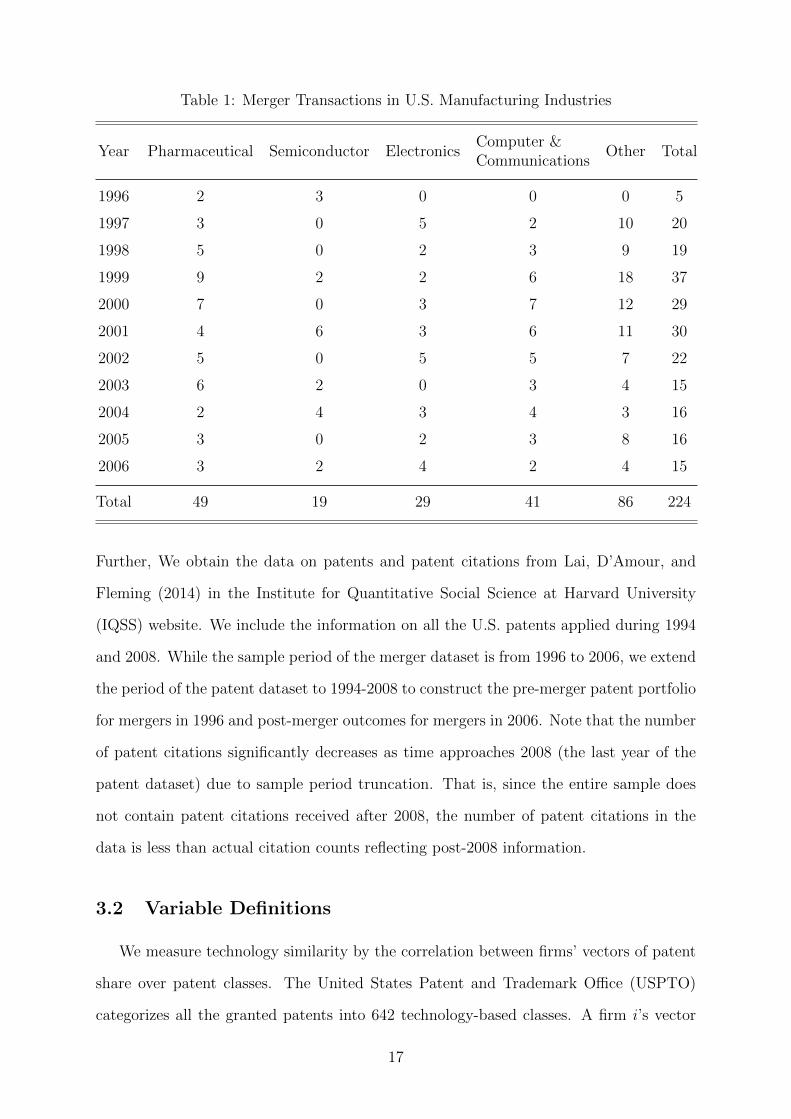
Table 1: Merger Transactions in U.S. Manufacturing Industries
Year Pharmaceutical Semiconductor ElectronicsComputer &Communications
Other Total
1996 2 3 0 0 0 5
1997 3 0 5 2 10 20
1998 5 0 2 3 9 19
1999 9 2 2 6 18 37
2000 7 0 3 7 12 29
2001 4 6 3 6 11 30
2002 5 0 5 5 7 22
2003 6 2 0 3 4 15
2004 2 4 3 4 3 16
2005 3 0 2 3 8 16
2006 3 2 4 2 4 15
Total 49 19 29 41 86 224
Further, We obtain the data on patents and patent citations from Lai, D’Amour, and
Fleming (2014) in the Institute for Quantitative Social Science at Harvard University
(IQSS) website. We include the information on all the U.S. patents applied during 1994
and 2008. While the sample period of the merger dataset is from 1996 to 2006, we extend
the period of the patent dataset to 1994-2008 to construct the pre-merger patent portfolio
for mergers in 1996 and post-merger outcomes for mergers in 2006. Note that the number
of patent citations significantly decreases as time approaches 2008 (the last year of the
patent dataset) due to sample period truncation. That is, since the entire sample does
not contain patent citations received after 2008, the number of patent citations in the
data is less than actual citation counts reflecting post-2008 information.
3.2 Variable Definitions
We measure technology similarity by the correlation between firms’ vectors of patent
share over patent classes. The United States Patent and Trademark Office (USPTO)
categorizes all the granted patents into 642 technology-based classes. A firm i’s vector
17

of patent shares over classes is represented by Fi = (Fi,1, Fi,2, ..., Fi,642), where Fi,c is
a firm i’s ratio of patent counts in class c to the total number of patents. Following
Jaffe (1986), the technological similarity is measured by the correlation between merger
partners’ technologies as follows:
CR(FA, FT ) =Cov(FA, FT )√
Var(FA) · Var(FT ), (10)
where FA (FT ) represents acquirer A’s (target T ’s) vector of patent shares over patent
classes. Some previous studies construct a measure of technology similarity by using this
patent distribution vector of firms. Ozcan (2015) measures technology similarity for his
sample of industrial firms with the Euclidean distance between merging firms’ vectors of
patent share over patent classes, whereas Linde and Siebert (2016) measure technology
similarity for their firms in the U.S. semiconductor industry by using the correlation
between merging firms’ vectors of patent share over patent classes. We use the correlation
(CR) between pre-merger patent distribution vectors of two firms to measures technology
similarity between firms, which is consistent with Linde and Siebert (2016). Two firms
have more similar technologies before their merger when CR is higher.
We measure technological complementarity by Mahalanobis distance (MAHA) be-
tween firms following Bloom et al. (2013). First, contruct a matrix of every firm’s vector
of patent shares over technology classes. That is, the 642×N matrix, F = [F ′1, F
′2, ..., F
′N ],
is the matrix of all the firms’ patent distributional vectors over 642 classes, where Fi
is a firm i’s 1 × 642 vector of patent shares across classes and N is the total num-
ber of firms. Then, normalize each column of the matrix F , so that obtain another
matrix F = [F ′1
(F1F ′1)
1/2 ,F ′2
(F2F ′2)
1/2 , ...,F ′N
(FNF′N )1/2
]. Third, form the N × 642 matrix C =
[F ′(,1), F
′(,2), ..., F
′(,642)], where F(,c) is a class c’s 1 × N vector of patent shares over N
firms. Then, C = [F ′(,1)
(F(,1)F′(,1)
)1/2,
F ′(,2)
(F(,2)F′(,2)
)1/2, ...,
F ′(,642)
(F(,642)F′(,642)
)1/2] is the normalized N × N
matrix of C. Thus, the 642 × 642 matrix CCORR = C ′C indicates the uncentered
correlation between vectors of all the classes’ patent shares across firms. Finally, to cap-
ture technological relatedness between different patent classes, use the N × N matrix
TECHSPILL = F ′ × CCORR × F . Hence, each element of the TECHSPILL matrix is
18

the MAHA distance between two corresponding firms. Therefore, MAHA is the weighted
correlation between firms’ patent class distributional vectors, where the weight is defined
by the correlation among all the patent classes (CCORR).
Technology similarity assumes that the spillovers occur only within the same patent
class, thus ruling out spillovers between different classes. In particular, CR partitions
technology space according to 642 patent classes, and it assumes that patent classes
are orthogonal to each other. As a result, in the case that two firms have no patent
filed in overlapping classes, the spillover effect between the two would be assigned as
zero. However, knowledge could flow not only within a class, but also across classes.
Therefore, MAHA is better in reflecting knowledge complementary across different patent
classes. We illustrate the difference between CR and MAHA with the following exam-
ple. Suppose that there are only 3 patent classes, and that acquirer A’s and target T ’s
vectors of patent shares over 3 classes are FA = (0.1, 0.4, 0.5) and FT = (0, 0.8, 0.2).
The correlation between two merger partners’ technologies A and T (CRAT ) is 0.5. To
compute MAHA, we take the following steps. Consider F = [F ′A, F
′T ] =
0.1 0
0.4 0.8
0.5 0.2
,
so that F =[
F ′A
(FAF′A)1/2
,F ′T
(FTF′T )1/2
]=
0.15 0
0.62 0.97
0.77 0.24
. Moreover, C = [F ′(,1), F
′(,2), F
′(,3)] =
0.1 0.4 0.5
0 0.8 0.2
, and C =
[F ′(,1)
(F(,1)F′(,1)
)1/2,
F ′(,2)
(F(,2)F′(,2)
)1/2,
F ′(,3)
(F(,3)F′(,3)
)1/2
]=
1 0.45 0.93
0 0.89 0.37
. Thus,
the matrix CCORR = C ′C =
1 0.45 0.93
0.45 1 0.75
0.93 0.75 1
. Finally, the matrix TECHSPILL =
F ′ × CCORR × F =
2.02 1.56
1.56 1.35
, so that Mahalanobis distance between two merger
partners A and T (MAHAAT ) is 1.56.
We measure product similarity by the correlation between firms’ vectors of sales share
19

over business segments. The Compustat provides the information of each firm’s business
segments classified by 4 digit SIC. We construct each firm’s pre-merger sales distribution
over 216 business segments based on the product market segment data. That is, a firm i’s
vector of sales across business segments is denoted by Si = (Si,1, Si,2, ..., Si,216), where Si,b
is a firm i’s ratio of sales in a business segment b to the total sales before the merger. The
PCR is the correlation between the pre-merger sales distribution vectors of two firms,
which measures product market similarity between them. Two firms are more likely to
compete in similar product markets before their merger when PCR is higher. Further,
we measure product complementarity by PMAHA, which is the correlation among firms’
vectors of market share in various business segments weighted by the correlation across
those business segments.
Turning to the post-merger outcomes, we use the average of a firm’s Tobin’s Q during
1 year (TOBINQ) and 3 years (AVERQ) after merger as measures of short-run and
long-run valuation effects, respectively. There have been several attempts to explore the
relationship between R&D or patents and stock market value (Hall, 2000; Hall, B. H.,
Jaffe, A., & Trajtenberg, 2005; Pakes, 1985). According to those studies, other measures
such as profit or total factor productivity (TFP) do not precisely reflect value of R&D
inputs (e.g., technologies) or R&D outputs (e.g., patents, citations, or products). On the
other hand, Tobin’s Q is a better indicator of expected net present value generated by
those factors related to R&D.
We employ total patent counts (PAT) and a total number of citation-weighted patents
(CWP) during 3 years after merger as measures of post-merger innovation outcomes.
Many researchers use patent counts as a proxy of innovation output (Ahuja & Katila,
2001; Benner & Waldfogel, 2008; Fleming, 2001; Hausman, Hall, & Griliches, 1984; Or-
naghi, 2009). However, each patent has different technological influence or economic
value. In this case, the number of citation-weighted patents can be an alternative measure
to simple patent counts in the sense that the number of citations to a patent represents
the patent’s value (Hall, B. H., Jaffe, A., & Trajtenberg, 2005; Trajtenberg, 1990). For in-
stance, a patent cited by other 100 patents is more valuable than another patent without
20

citations because the former is technologically more influential to other patents than the
latter. In order to construct citation-weighted patent counts, we apply the linear weight-
ing scheme to the analysis following Trajtenberg (1990). That is, let a firm i’s number of
citations received for each patent k be CITik, then the firm i’s citation-weighted patent
counts (CWPi) become
CWPi =n∑k=1
(1 + CITik), (11)
where n is the number of patents granted to the firm i. For our analysis, we use the number
of patents to measure the quantity of innovation outputs and the citation-weighted patent
counts to measure the quality of innovation outputs. Additionally, we compute the ratio
of citation to patent (CITINT) to measure the average quality of patent.
In addition to patent count, citation-weighted patents and citation per patent, we
consider the following post-merger innovation outcomes: (1) the 90 percentile of orig-
inality of patents (ORIG), (2) the 90 percentile of generality of patents (GENERAL),
and (3) the standard deviation of CWP during 3 years after merger (STDV). Specifically,
we employ originality and generality index provided by National Bureau of Economic
Research (NBER) Patent Data Project website. Following Hall, Jaffe, and Trajtenberg
(2001), the measure of originality (generality) is constructed by Measurei = 1−∑C
c s2ic,
where sic indicates the ratio of citations made (received) by patent i in patent class c
to C patent classes. While ORIG and GENERAL measure technological diversity after
merger (Hall et al., 2001), STDV measures the risk of post-merger patenting activity
(Amore, Schneider, & Zaldokas, 2013).
3.3 Descriptive Statistics
Table 2 reports the descriptive statistics. All financial variables are adjusted to dollar
values in 2000 using consumer price index (CPI). Target firms show higher R&D inten-
sity than acquirers, which is consistent with the results in Blonigen and Taylor (2000).
Moreover, acquirers have larger stock market values than targets, so that they are more
21

Table 2: Descriptive Statistics
Variable Description Mean Std. Dev. N
Acquirer
R&D intensity log
(R&D expenditure
Sales
)0.166 0.266 224
Tobin’s Q log
(Stock market value
Total asset
)1.104 0.126 224
IND1 Pharmaceutical Industry 0.232 0.423 224
IND2 Semiconductor Industry 0.103 0.304 224
IND3 Electrionics Industry 0.107 0.310 224
IND4 Computer & Communications Industry 0.161 0.368 224
IND5 Other Industry 0.397 0.490 224
Target
R&D intensity log
(R&D expenditure
Sales
)0.341 0.615 224
Tobin’s Q log
(Stock market value
Total asset
)1.092 0.196 224
IND1 Pharmaceutical Industry 0.219 0.414 224
IND2 Semiconductor Industry 0.085 0.279 224
IND3 Electrionics Industry 0.129 0.336 224
IND4 Computer & Communications Industry 0.183 0.388 224
IND5 Other Industry 0.384 0.487 224
Match-SpecificCharacteristic
CR Correlation distance of technologies 0.382 0.313 224
MAHA Mahalanobis distance of technologies 0.941 0.598 224
PCR Correlation distance of products 0.436 0.467 224
PMAHA Mahalanobis distance of products 0.352 0.356 224
SameState Dummy for same state 0.402 0.491 224
Post-MergerOutcome
TOBINQ1 Tobin’s Q in merger year 1.032 0.497 224
TOBINQ3 3-year average of Tobin’s Q after merger 0.966 0.442 224
PAT log(Patent counts) 3.727 1.941 224
CWP log(Citation-weighted patent counts) 4.778 2.445 224
CITINT log
(CitationsPatents
)0.939 0.811 224
ORIG Originality of patents 0.588 0.342 224
GENERAL Generality of patents 0.460 0.390 224
STDV 3- year standard deviation of CWP after merger 10.435 6.131 224
22

capable to finance a merger. Before taking a logarithm, the average of acquirers’ stock
market value before merger is about $16 billion, whereas the average of targets’ stock
market value is approximately $2.3 billion. The average Tobin’s Q of acquirers is slightly
higher than that of targets. The composition of targets’ industry is similar to that of
acquirers’ industry because most of the deals are horizontal mergers. Pharmaceutical
firms involve in more merger transactions than firms in the other manufacturing sectors.
In particular, more than 20% of mergers belong to pharmaceutical industry.
Turning to the match-specific characteristics, which play the key role in merger value
function. The averages of CR and MAHA are 0.382 and 0.941, respectively. The averages
of PCR and PMAHA are 0.436 and 0.352, respectively. 40.2% of our mergers with the
acquirer and target locating in the same state. Finally, the descriptive statistics of post-
merger outcomes are presented in the bottom panel of Table 2.
4 Empirical Results
4.1 Matching Model Estimation
This sub-section discusses the results of merger value function reported in Table 3.
First, the coefficients for CR and PCR are positive and significant in Column (1), and the
coefficients for MAHA and PMAHA are positive and significant in Column (2). These
results indicate that the more similar the merger partners’ technologies and products,
the higher their merger value. These results suggest that technology spillover and prod-
uct market synergies between merging firms create merger value. Our results support
Hypotheses 1 and 2.
Turning to the control variables, we find that a firm with high Tobin’s Q derives more
value from another high Q firm, indicating a positive assortative matching in Tobin’s Q.
This is supported by the fact that we obtain more maximum score inequalities satisfied
by setting the coefficient for an interaction term between merging partners’ Tobin’s Q
to +1 instead of -1. It implies that merging partners with higher level of Tobin’s Q can
create larger synergies through the merger (Rhodes-Kropf & Robinson, 2008).
23

Tab
le3:
Mer
ger
Val
ue
Est
imat
ion
(1)
(2)
(3)
(4)
(5)
(6)
(7)
(8)
MA
HA
95.2
73**
95.8
57**
64.1
16**
[35.
333,
95.3
02]
[35.3
23,
94.7
03]
[23.9
73,
86.9
25]
[,]
PM
AH
A79
.635
**74.0
76**
77.1
04**
[25.
541,
93.3
70]
[31.2
47,
91.6
19]
[25.8
89,
91.1
78]
[,]
CR
69.2
91**
65.0
42**
82.7
62**
[27.
282,
88.4
26]
[26.0
81,
87.0
19]
[32.4
28,
93.1
97]
[,]
PC
R22
.259
**22.4
83**
83.4
57**
[14.
775,
74.4
87]
[11.4
56,
74.2
44]
[30.2
39,
91.0
65]
[,]
Sam
eSta
te3.
288
16.6
763.2
27
7.5
83
12.1
93
10.9
84
[-27
.897
,15
.920
][-
25.6
19,
39.2
62]
[-9.7
82,
45.3
80]
[-25.2
83,
59.2
99]
[-11.2
96,
52.1
44]
[-18.9
76,
60.6
79]
[,]
[,]
Tob
in′ s
Qat
1**
1**
1**
1**
1**
1**
1**
1**
Nor
mal
ized
Nor
mal
ized
Norm
alize
dN
orm
ali
zed
Norm
ali
zed
Norm
ali
zed
Norm
ali
zed
Norm
ali
zed
R&
Din
ten
sity
at
7.34
22.
167
94.3
91
42.7
31
87.4
34
42.5
34
[-30
.527
,68
.776
][-
31.2
43,
66.1
19]
[-3.5
20,
90.8
56]
[-15.6
38,
79.4
97]
[-2.5
54,
94.1
70]
[-15.0
30,
79.7
19]
[,]
[,]
Ineq
ual
itie
s2,
684
2,68
43,0
64
3,0
64
671
671
13,2
50
13,2
50
%of
Ineq
.sa
tisfi
ed71
.76%
71.6
8%72.5
8%
72.6
9%
88.8
2%
90.3
1%
%%
Mer
ger
mar
ket
s46
4641
41
46
46
46
46
Note:
We
use
the
max
imu
msc
ore
esti
mat
ion
inal
lth
eco
lum
ns
an
dru
nth
ees
tim
ati
on
firs
tse
ttin
gth
eco
effici
ent
for
an
inte
ract
ion
term
bet
wee
nm
ergin
gfi
rms’
Tob
in’s
Qto
+1,
and
then
fixin
git
to-1
.W
eth
ense
lect
the
vec
tors
of
para
met
eres
tim
ate
sth
at
maxim
ize
the
maxim
um
score
ob
ject
ive
fun
ctio
n.
Th
ese
lect
edco
effici
ent
for
the
inte
ract
ion
term
ofT
obin
’sq
(Tob
in′ s
Qat)
is+
1.
R&
Din
ten
sity
at
isth
ein
tera
ctio
nte
rmb
etw
een
acq
uir
er’s
an
dta
rget
firm
’sR
&D
inte
nsi
ty.
95%
con
fiden
cein
terv
alis
show
nin
bra
cket
s.T
he
coeffi
cien
tsare
sign
ifica
nt
at
the
5%
leve
lw
hen
the
con
fid
ence
inte
rval
does
not
conta
in0.
Mer
ger
mark
etis
defi
ned
by
the
com
bin
atio
nof
targ
etfi
rms’
ind
ust
ryty
pe
an
dm
erger
tran
sact
ion
year
inC
olu
mn
s(1
),(2
),(5
)to
(8).
For
Colu
mn
s(3
)an
d(4
),m
erger
mark
etis
con
stru
cted
by
usi
ng
acqu
irin
gfi
rms’
ind
ust
ryty
pe
an
dm
erger
year.
**p<
0.0
5
24

Furthermore, since the coefficient for the interaction term of Tobin’s Q is normalized
to +1, we measure the relative importance of each covariate in generating merger value.
In Table 4, we multiply one standard deviation of each covariate to its corresponding
point estimate reported in Columns (1) and (2) of Table 3 for comparison. According to
the results, MAHA has the largest impact in creating merger value, and then followed by
PMAHA. That is, when we increase MAHA by one standard deviation (0.51), the merger
value rises by 48.59. The increase in one standard deviation of PMAHA (0.26) raises
the merger value by 20.71. On the other hand, an increase in one standard deviation
of CR and PCR raises the match value by 17.25 and 7.81, respectively. The impact
of MAHA is three times larger than that of CR, which suggests that the technology
spillover across and within patent classes are both important to create merger value.
The impact of PMAHA is four times larger than that of PCR, which suggests that the
product market synergies from reducing competitiona and from internalizing externality
across complementary products are both important to create merger value. Furthermore,
when there is an increase in one standard deviation (0.266) of interaction term between
merging firms’ Tobin’s Q, the merger value increases by 0.266, only about 0.5% of the
rise in the merger value due to the changes in MAHA.
25

Tab
le4:
Rel
ativ
eIm
por
tance
ofC
ovar
iate
sin
Mat
chV
alue
(1)
(2)
(3)
(4)
(5)
(6)
(7)
(8)
(9)
Est
.S
td.
Dev
.E
st.×
Std
.D
ev.
Est
.S
td.
Dev
.E
st.×
Std
.D
ev.
Est
.S
td.
Dev
.E
st.×
Std
.D
ev.
CR
69.2
90.
2517.2
565.0
40.2
516.2
682.7
60.2
520.6
9
PC
R22
.26
0.35
7.8
122.4
80.3
57.8
783.4
60.3
529.2
1
MA
HA
95.2
70.
5148.5
995.8
60.5
148.8
964.1
20.5
132.7
PM
AH
A79
.64
0.26
20.7
174.0
80.2
619.2
677.1
0.2
620.0
5
Tob
in’s
Qat
10.
266
0.2
66
10.2
66
0.2
66
10.2
66
0.2
66
Note:
Est
.in
dic
ates
ap
oint
esti
mate
of
each
cova
riate
inT
ab
le3.
Poin
tes
tim
ate
sin
Colu
mn
(1)
com
efr
omC
olu
mn
(1)
and
(2)
inT
ab
le3,
those
inC
olu
mn
(4)
are
from
Colu
mn
(3)
an
d(4
)in
Tab
le3,
an
dth
ose
inC
olu
mn
(7)
com
efr
omC
olu
mn
(5)
an
d(6
)in
Tab
le3.
Tob
in′ s
Qat
isth
ein
tera
ctio
nte
rmb
etw
een
acqu
irer
’san
dta
rget
firm
’sT
obin
’sQ
.
26

Finally, we examine the goodness-of-fit of our matching model. To this end, we
compare the acquirer-target pairs in a stable matching equilibrium with those in observed
matching. When the stable matching assignments are similar to the realized merger
pairs, the empirical matching model has a predictive power. The procedure of generating
predicted matches from our model is as follows. First, we use the estimated coefficients
reported in Column 2 of Table 3 to compute all the possible merger values. Then, deferred
acceptance algorithm based on these match values is applied to matching games in all
the merger markets to find pairwise stable matching assignments.
Table 5: Year-by-Year Goodness-of-Fit
YearNumber of
MergersPredictedMatch (1)
PredictionRate (%)
AverageRank
PredictedMatch (2)
PredictionRate (%)
AverageRank
1996 5 0 0% 72% 1 40% 75%
1997 21 6 29% 58% 8 40% 74%
1998 18 10 56% 70% 12 68% 66%
1999 37 7 19% 69% 8 41% 74%
2000 29 18 62% 62% 16 55% 75%
2001 30 9 30% 65% 12 47% 67%
2002 22 8 36% 71% 7 41% 75%
2003 16 11 60% 76% 11 60% 81%
2004 15 6 40% 70% 9 50% 76%
2005 17 13 76% 71% 10 75% 77%
2006 14 8 57% 68% 7 73% 75%
Total 224 96 43% 68% 101 45% 74%
Note: Predicted Match (1) represents the number of observed matches consistent with equilib-rium matches driven by the match values computed using estimiates in Column (1) of Table3. Predicted Match (2) represents the number of observed matches consistent with equilib-rium matches driven by the match values computed using estimiates in Column (2) of Table 3.Average Rank indicates the percentile of realized merger matches relative to values of all thecounterfactual matches.
Table 5 shows the goodness-of-fit of our model by year. Finally, we compare the
merger matches in the stable matching equilibrium and those observed in the data. Our
model predicts 101 mergers among 224 transactions, indicating 45% of prediction rate.
Except for 1996 and 1999, the merger prediction rate of the model is more than 50%.
27

When it comes to the highest value, there are 117 mergers having the merger value higher
than all counterfactual mergers. This implies that some acquirer purchases a target firm
with lower match value. It is because the acquiring firm’s potential target with the highest
value is matched to another acquirer who provides a higher offer to the target.
4.2 Model Extension
4.2.1 Alternative Market Definition
The first extension is on the specific merger market definition used in our benchmark
model. In this robustness check, we define the merger market as the combination of
acquirer’s industry types and merger transaction year. We report the results from this
alternative market definition in Column (3) and (4) of Table 3. Encouragingly, they are
qualitatively similar to the results in Column (1) and (2) of Table 3. The coefficients of CR
and PCR are positive and significant in Column (1), and the coefficients of MAHA and
PMAHA are positive and significant in Column (2). Both model specifications suggest
that technology spillover and product market synergies create merger value.
4.2.2 Predetermination of Acquirer and Target Sets
Columns (5) and (6) in Table 3 reports the estimation results for this robustness check.
The coefficient of PMAHA is positive and significant, suggesting that complementarity in
merging firms’ products increases merger value. Further, the coefficient of CR is positive
and significant. However, the percentage of stable equilibrium inequalities satisfied only
71.68% in this robustness check, which is lower than 91.12% in the benchmark model.
These results indicate that our benchmark model is more appropriate to explain the
merger partner choices than the model using extended sets of acquirers and target firms.
We interpret these results as the choice of being either acquirer or target is driven by
acquirer- or target-specific characteristics rather than match-specific characteristics.
28

4.2.3 Merging or Staying Independent
The third model extension is to include non-merging firms into the sample. Before
choosing a merger partner, a firm decides whether to merge or to stay alone. Then, it
chooses to merge with a firm that is expected to achieve synergies. By including stand-
alone firms in our sample, we alleviate the endogeneity problem caused by the correlation
between unobservables driving merger partner choice and merger decision.
The following example shows how to construct maximum score inequalities in this
case. Suppose that there are 5 firms in a merger market, 2 acquirers a and a, 2 targets
t and t and a nonmerging firm s. Their matching outcomes are (a, t), (a, t) ∈ µ and
s ∈ SA, where SA represents a set of stand-alone firms. For two realized merger pairs
(a, t) and (a, t), we use the inequality (5) to determine whether they belong to stable
matching equilibrium. However, to compare match value between observed merger pairs
and a stand-alone firm, we impose the following assumptions. First, we assume that a
non-merging firm’s similarity and complementarity of technology and product are zero.
It is because those distances cannot be defined for a stand-alone firm. Second, we set
the interaction term of R&D intensity and Tobin’s Q to individual firm’s characteristics.
Based on these assumptions, a stable matching inequality can be written as
V (a, t) + V (s, 0) ≥ V (a, 0) + V (s, t), (12)
where (s, 0) and (a, 0) represent stand-alone firms. Even though a stand-alone firm s
plays a role as an acquirer in Equation (13), it can also be acquired by another firm.
Thus, we can construct an additional inequality
V (a, t) + V (0, s) ≥ V (a, s) + V (0, t). (13)
When it comes to two non-merging firms s1 and s2, they prefer to be stand-alone firms
rather than merging with each other. This implies the following inequality
V (s1, 0) + V (s2, 0) ≥ V (s1, s2). (14)
29

Taken together, our maximum score objective function becomes
Q(α) =n∑
m=1
{ ∑s,s1,s2∈SAm
∑(a,t),(a,t)∈µm
1
[{q1(α) ≥ 0} ∩ {q2(α) ≥ 0}
]
+1
[{q3(α) ≥ 0} ∩ {q4(α) ≥ 0}
]+ 1[q5(α) ≥ 0] + 1[q6(α) ≥ 0]
}, (15)
where q1(α) = V (a, t|α) + V (a, t|α)− V (a, t|α)− V (a, t|α)
q2(α) = V (a, t|α) + V (s, 0|α)− V (a, 0|α)− V (s, t|α),
q3(α) = V (a, t|α) + V (0, s|α)− V (a, s|α)− V (0, t|α),
q4(α) = V (a, t|α) + V (s, 0|α)− V (a, 0|α)− V (s, t|α),
q5(α) = V (a, t|α) + V (0, s|α)− V (a, s|α)− V (0, t|α),
q6(α) = V (s1, 0|α) + V (s2, 0|α)− V (s1, s2|α), .
Columns (7) and (8) of Table 3 present the results for the model including stand-
alone firms into the sample. Being consistent with our benchmark estimation results,
the coefficient of MAHA is positive and significant, suggesting that complementarity in
merging firms’ technologies plays a positive role in selecting to merger and whom to
merger with. More importantly, containing stand-alone firms into the sample allows us
to pin down the effect of technology complementarity on merger value more precisely. As
a result, we obtain a larger estimate of MAHA relative to the estimate in Column 5 of
Table 3.
4.3 Counterfactual Analysis
In this sub-section, we perform counterfactual experiments exploring changes in merger
value function when technology and product complementarities are assumed to have no
effect on merger value function. In other words, our counterfactual experiments examine
characteristics of the matches in a stable equilibrium if firms do not consider similarity or
complementarity in technology and product as a determinant of merger value function.
Table 6 shows the results of these counterfactual experiments. First, we turn the
30

Tab
le6:
Cou
nte
rfac
tual
Anal
ysi
s
(1)
(2)
(3)
(4)
(5)
(6)
CR
MA
HA
PC
RP
MA
HA
%d
rop
inm
atch
valu
eP
red
icti
on
rate
(%)
Bas
elin
eM
od
el(1
)0.
471
0.5
0%42.9
%
αCR
=0
0.25
90.
487
46.1
%39.1
%
αPCR
=0
0.38
70.
292
14.8
%40.2
%
αCR
=0
&αPCR
=0
0.24
40.
243
51.7
%34.9
%
Bas
elin
eM
od
el(2
)1.
042
0.41
60%
45.1
%
αMAHA
=0
0.80
90.
454
66.8
%30.4
%
αPMAHA
=0
0.99
50.
229
24.5
%38.1
%
αMAHA
=0
&αPMAHA
=0
0.69
00.
188
75.2
%21.6
%
Note:αCR
,αM
AHA
,αPCR
andαPM
AHA
ind
icate
an
esti
mate
dco
effici
ent
for
CR
,M
AH
A,
PC
Ran
dP
MA
HA
resp
ecti
vel
y.W
ed
oea
chco
unte
rfac
tual
exp
erim
ent
by
sett
ing
corr
esp
on
din
gp
ara
met
eres
tim
ate
inth
eb
asel
ine
mod
elto
0an
dfi
nd
-in
gst
able
equ
ilib
rium
mat
ches
bas
edon
def
erre
dacc
epta
nce
alg
ori
thm
.C
R,
MA
HA
,P
CR
an
dP
MA
HA
are
the
aver
ages
ofth
ose
mea
sure
sof
all
the
equ
ilib
riu
mm
atc
hes
inea
chco
unte
rfact
ual
exp
erim
ent.
%d
rop
inm
atc
hva
lue
rep
rese
nts
%d
ecre
ase
insu
mof
mat
chva
lues
from
equ
ilib
riu
mm
atc
hes
inea
chco
unte
rfact
ual
exp
erim
ent
com
pare
dto
valu
esu
mof
equ
ilib
riu
mm
atch
esin
our
bas
elin
em
od
el.
31

coefficient of MAHA to zero and compute the stable equilibrium matches. The average
of technology similarity in equilibrium matches decreases from 0.402 in the benchmark
model to 0.259 in this counterfactual experiment, and the average of technology com-
plementarity in equilibrium matches decreases from 0.975 in the benchmark model to
0.712 in this counterfactual experiment. The reductions of CR and MAHA in equilib-
rium matches from the benchmark and this counterfactual experiment are 0.14 and 0.26,
which are equivalent to 46% and 44% of one standard deviation of those measures, respec-
tively. Firms select merger partners with less complementary technologies if technology
complementarity does not appear in the merger value function. More importantly, when
it comes to a decrease in match values in this counterfactual experiment, it shows about
46.1% reduction in value sum of equilibrium matches relative to value sum from baseline
equilibrium matches. The prediction rate of our model for observed merger decreases from
64.7% to 41.1%. These results suggest that the inclusion of technology complementarity
is significantly important to explain merger partner choices.
Second, we turn the coefficient of PMAHA to zero and compute the stable equilib-
rium matches. The reductions of PCR and PMAHA in equilibrium matches from the
benchmark and this counterfactual experiment are 0.06 and 0.05, which are equivalent
to 13% and 15% of one standard deviation of those measures, respectively. Firms select
merger partners with less complementary products if they do not concern about product
complementarity in the merger value function. Moreover, the counterfactual model gen-
erates 14.5% lower merger value and predicts 7.6% fewer realized matches among entire
observed matches. These results imply that product complementarity also plays a crucial
role in merger partner choices.
4.4 Post-Merger Outcomes
The choice of merger partner is made under the expectation of mutual gain. The
probability of merger between firms with complementary technologies and products is
higher because they expect a greater synergy from combining those resources. An im-
portant aspect of merger synergy for creating value is the post-merger innovation. Thus,
32

the merger value is expected to be positively related to those post-merger outcomes if
the anticipated merger synergy realized. Such relationship also provides a support for
the specification of our model.
In this sub-section, we regress the post-merger outcomes on the estimated merger
value. The regressions also control for year and industry fixed effects as well as acquirer-
and target-specific attributes. Thus, the post-merger outcome equation is
Yi = β1Vi +Xaiβ2 +Xtiβ3 + νyear + ξindustry + εi, (16)
where Yi represents a merged firm i’s post-merger outcome variables. Vi is the firm i’s
estimated merger value. Xai and Xti are acquirer- and target-specific characteristics,
respectively. νyear represents year fixed effects, ξindustry represents industry fixed effects,
and εi is an unobserved error term.
Table 7 reports the relationship between post-merger outcomes and estimated merger
value, where the estimated merger value is based on Column (5) of Table 3. First, we
examine how the merger value relates to post-merger valuation in stock market. We
use two different types of Tobin’s Q to measure the merged firm’s short- and long-run
valuations based on the expectation of discounted present value. The coefficients in
Column (1) and (2) are positive and significant, suggesting that the merger value has
positive influences in the firm’s valuation in the merger year and over the three-year
period after the merger, respectively. Taken together, the merger value positively relates
to the merged firm’s short- and long-run valuations.
Next, we turn to the relationship between estimated merger value and post-merger
innovation outcomes. The coefficients on the merger value are positive and significant in
Columns (3) to (4) of Table 7. These results indicate that the larger the merger value,
the more patents and citations after the merger. In addition, the coefficient in Column
(5) is positive, suggesting that the merger value is more related to innovation quality
than innovation quantity.
The estimates of match value are positive and significant in Columns (6) and (7). It
suggests that the merger value is positively correlated with originality and generality of
33

Table 7: Post-Merger Outcomes
(1) (2) (3) (4) (5) (6) (7) (8)TOBINQ AVERQ PAT CWP CITINT ORIG GENERAL STDV
Match Value 0.0439 0.0405* 0.503*** 0.573*** 0.0552† 0.0418* 0.0364* 0.0568*(0.0267) (0.0161) (0.107) (0.120) (0.0299) (0.0163) (0.0179) (0.0274)
Acquirer
R&D intensity 0.122 0.0724 -0.711 -0.997 -0.239 0.0664 0.120 -0.309*(0.148) (0.0892) (0.589) (0.662) (0.165) (0.0896) (0.0985) (0.151)
Tobin’s Q -3.735*** -3.458** 0.500 -0.298 -0.276 -0.471(1.087) (1.222) (0.304) (0.165) (0.182) (0.278)
Target
R&D intensity 0.0719 0.0723 -0.194 -0.126 0.0894 0.0131 -0.0150 0.131(0.0667) (0.0401) (0.265) (0.298) (0.0741) (0.0403) (0.0444) (0.0678)
Tobin’s Q 0.335 0.339 0.0677 0.132 0.140 0.164(0.712) (0.801) (0.199) (0.108) (0.119) (0.182)
Year effects YES YES YES YES YES YES YES YES
Industry effects YES YES YES YES YES YES YES YES
Observations 224 224 224 224 224 224 224 224
Adjusted R2 0.235 0.242 0.225 0.382 0.653 0.421 0.461 0.072
Note: Robust standard errors are in parentheses. We use OLS estimation in all the columns. The de-pendent variables are as follows. Tobin’s Q in a merger year (TOBINQ) in Column (1). The average ofpost-merger Tobin’s Q (AVERQ) in Column (2). The logged number of patents (PAT) in Column (3).The logged number of citation-weighted patents (CWP) in Column (4). The ratio of citation counts topatent counts (CITINT) in Column (5). The 90 percentile of originality of patents (ORIG) in Column(6). The 90 percentile of generality of patents (GENERAL) in Column (7). The standard deviation ofCWP during 3 years after merger (STDV) in Column (8). The Match Value is computed using the esti-mated parameters in Column (6) of Table 3.† p < 0.10, * p < 0.05, ** p < 0.01, *** p < 0.001
technological diversity, and patenting volatility.
Further, since Table 4 reports that technology complementarity (i.e. MAHA) and
product complementarity (i.e PMAHA) are two important elements in the merger value
function, we examine their economic impacts on the post-merger outcomes. We rank the
observed mergers according to their MAHA and PMAHA values. Then, we examine the
post-merger outcomes for the group of mergers with MAHA and PMAHA in first quarter
and the group of mergers with MAHA and PMAHA in last quarter. We interpret mergers
with higher MAHA and PMAHA values as good matches, whereas mergers with lower
MAHA and PMAHA values as bad matches.
Table 8 shows the difference in post-merger outcomes between two merger groups with
34

Tab
le8:
Mer
ger
Val
ue
and
Pos
t-M
erge
rO
utc
omes
by
Diff
eren
tSim
ilar
ity
(1)
(2)
(3)
(4)
(5)
(6)
(7)
(8)
(9)
Mat
chV
alu
eT
OB
INQ
AV
ER
QP
AT
CW
PC
ITIN
TO
RIG
GE
NE
RA
LS
TD
V
Diff
eren
ceb
etw
een
Hig
han
dL
owC
Rgr
oup
64.8
2***
0.26
1**
0.30
7***
0.68
5*0.
554
-0.0
780.0
65
0.0
14
0.2
07†
(2.4
1)(0
.11)
(0.0
9)(0
.40)
(0.4
8)(0
.13)
(0.0
6)
(0.0
7)
(0.0
8)
Diff
eren
ceb
etw
een
Hig
han
dL
owP
CR
grou
p42
.46*
**0.
356*
*0.
332*
**-0
.439
-0.5
03-0
.022
0.0
37
-0.0
72
0.0
71
(3.3
5)(0
.09)
(0.0
7)(0
.37)
(0.4
8)(0
.15)
(0.0
7)
(0.0
7)
(0.0
8)
Diff
eren
ceb
etw
een
Hig
han
dL
owM
AH
Agr
oup
164.
80**
*0.
160*
0.18
7*1.
779*
**1.
816*
**0.
056
0.1
25*
0.0
65
0.2
00*
(8.0
4)(0
.09)
(0.0
8)(0
.40)
(0.5
0)(0
.15)
(0.0
6)
(0.0
7)
(0.0
9)
Diff
eren
ceb
etw
een
Hig
han
dL
owP
MA
HA
grou
p10
4.42
***
0.05
80.
082
0.21
90.
087
-0.1
53-0
.070
-0.0
26
0.1
50*
(12.
07)
(0.0
9)(0
.07)
(0.4
0)(0
.48)
(0.1
4)(0
.06)
(0.0
6)
(0.0
9)
Note:
Rob
ust
stan
dar
der
rors
are
inp
aren
thes
es.
Mer
ger
valu
ean
dp
ost
-mer
ger
ou
tcom
esin
each
gro
up
of
mer
ger
sare
the
aver
age
of
56
obse
rvat
ion
sin
each
grou
p.
†p<
0.10,*p<
0.05
,**p<
0.01
,***p<
0.0
01
35

high and low MAHA and that between two merger groups between high and low PMAHA.
Column (1) reports that the merger value is greater for merger with a higher technology
complementarity. Column (3) shows that the group of mergers with high MAHA has
average Tobin’s Q by 14% points higher than the group of mergers with lower MAHA
over three-year periods after the merger. Moreover, most of the post-merger innovation
outcomes are significantly larger for the group of mergers with higher MAHA. These
results suggest that a better innovation outcome is a source of merger synergy for merger
driven by complementary technologies between merging partners. Further, when it comes
to the comparison between the mergers with high PMAHA and low PMAHA, the former
group of mergers has average Tobin’s Q by 10% points higher than the latter group of
mergers over three-year periods after the merger (see Column 3). However, there is no
significant difference for post-merger innovation outcomes between high and low PMAHA
groups. We suggest that mergers driven by complementary products between merging
firms may seek synergy in pricing coordination and cost reduction.
5 Conclusion
This paper examines the effects of complementarities between firms’ technology and
product on merger value creation. We find that firms prefer to match with the other
firm that has complementary technologies and produces complementary products. All
these results suggest that merging firms perceive complement technologies and products
as sources of merger synergy. Technology and product complementarities contribute a
substantial portion of value creation from merger and improve the predictive power of
our model. Post-merger innovation quantity, innovation quality, and firm valuation are
both higher for mergers with a higher estimated merger value, suggesting mutual benefits
for both the merging firms from assortative matching in complementary technologies and
products.
The managerial implication of our analysis highlights the importance of merging with
the right partner in addition to merging with a good partner. While our analysis does not
36

imply that mergers are in general patent and value creating, it does suggest that firms
within a merger market tend to sort into merger pairs in order to maximize post-merger
performance. Mergers between firms with complementary technologies and products are
expected to achieve synergy because there is a considerable boost in post-merger perfor-
mance. Since divestiture and consolidation after merger are costly processes, managers
would be wise to consider technology and product complementarities as two additional
factors for deciding a potential merger.
References
Ahuja, G., & Katila, R. (2001). Technological Acquisition and the Innovation Perfor-
mance of Acquiring Firms: A Longitudinal Study. Strategic Management Journal ,
22 (3), 197–220.
Akkus, O., Cookson, J. A., & Hortacsu, A. (2015). The Determinants of Bank Mergers :
A Revealed Preference Analysis The Determinants of Bank Mergers : A Revealed
Preference Analysis. Management Science, 62 (8), 2241–2258.
Amore, M. D., Schneider, C., & Zaldokas, A. (2013). Credit supply and corporate
innovation. Journal of Financial Economics , 109 (3), 835–855.
Bena, J., & Li, K. (2014). Corporate Innovations and Mergers and Acquisitions. The
Journal of Finance, LXIX (5), 1923–1960.
Benner, M., & Waldfogel, J. (2008). Close to you? Bias and precision in patent-based
measures of technological proximity. Research Policy , 37 (9), 1556–1567.
Bertrand, O. (2009). Effects of foreign acquisitions on R&D activity: Evidence from
firm-level data for France. Research Policy , 38 (6), 1021–1031.
Blonigen, B., & Taylor, C. (2000). R&D Intensity and Acquisitions in High-Technology:
Evidence from the US Electronic and Electrical Equipment Industries. Journal of
Industrial Economics , 48 (1), 47–70.
Bloom, N., Schankerman, M., & Reenen, J. V. (2013). Identifying Technology Spillovers
and Product Market Rivalry. Econometrica, 81 (4), 1347–1393.
37

Cassiman, B., Colombo, M. G., Garrone, P., & Veugelers, R. (2005). The impact of
M&A on the R&D process. Research Policy , 34 (2), 195–220.
Chondrakis, G. (2016). Unique synergies in technology acquisitions. Research Policy ,
45 (9), 1873–1889.
Christensen, C., Alton, R., Rising, C., & Waldeck, A. (2011). The Big Idea: The New
M&A Playbook. Harvard Business Review(March).
Cohen, W. M., & Levinthal, D. A. (1990). Absorptive Capacity : A New Perspective on
Learning and Innovation. Administrative Science Quarterly , 35 (1), 128–152.
Cournot, A.-A. (1838). Recherches sur Les Principes Mathematiques De La Theorie Des
Richesses. chez L. Hachette.
Delgado, M. A., Rodriguez-Poo, J. M., & Wolf, M. (2001). Subsampling Inference in Cube
Root Asymptotics with An Application to Manski’s Maximum Score Estimator.
Economics Letters , 73 (2), 241–250.
Desyllas, P., & Hughes, A. (2010). Do high technology acquirers become more innovative?
Research Policy , 39 (8), 1105–1121.
Erel, I., Liao, R. C., & Weisbach, M. S. (2012). Determinants of Cross-Border Mergers
and Acquisitions. The Journal of Finance, 67 (3), 1045–1082.
Fleming, L. (2001). Recombinant Uncertainty in Technological Search. Management
Science, 47 (1), 117–132.
Fox, J. T. (2010a). Estimating Matching Games with Transfers.
Fox, J. T. (2010b). Identification in matching games. Quantitative Economics , 1 (2),
203–254.
Gal-Or, E. (1988). The Informational Advantages or Disadvantages of Horizontal Merg-
ers. International Economic Review , 29 (4), 639–661.
Grossman, S., & Hart, O. D. (1986). The Costs and Benefits of Ownership : A Theory
of Vertical and Lateral Integration. Journal of Political Economy , 94 (4), 691–719.
Hall, B. H. (2000). Innovation and Market Value (R. Barrell, G. Mason, & M. O’Mahony,
Eds.). New York: Cambridge University Press.
Hall, B. H., Jaffe, A. B., & Trajtenberg, M. (2001). The NBER Patent Citation Data
38

File: Lessons, Insights and Methodological Tools.
Hall, B. H., Jaffe, A., & Trajtenberg, M. (2005). Market value and patent citations.
RAND Journal of Economics , 36 (1), 16–38.
Hausman, J., Hall, B. H. ., & Griliches, Z. (1984). Econometric Models for Count Data
with an Application to the Patents-R & D Relationship. Econometrica, 52 (4),
909–938.
Hoberg, G., & Phillips, G. (2010). Product Market Synergies and Competition in Mergers
and Acquisitions : A Text-Based Analysis. Review of Financial Studies , 23 (10),
3773–3811.
Ishihara, M., & Rietveld, J. (2017). The Effect of Acquisitions on Product Innovativeness
, Quality , and Sales Performance : Evidence from the Console Video Game.
Jaffe, A. (1986). Technological Opportunity and Spillovers of R&D : Evidence from
Firms ’ Patents , Profits , and Market Value. American Economic Review , 76 (5),
984–1001.
Jensen, M. C. (1988). Takeovers : Their Causes and Consequences. Journal of Economic
Perspective, 2 (1), 21–48.
Lai, R., D’Amour, A., & Fleming, L. (2014). The careers and co-authorship networks of
U.S. patent-holders, since 1975. doi: hdl/1902.1/12367
Linde, S., & Siebert, R. (2016). Do Mergers Among Multimarket Firms Create Value?
Makri, M., Hitt, M. A., & Lane, P. J. (2010). Complementary Technologies, Knowledge
Relatedness, and Invention Outcomes in High Technology Mergers and Acquisitions.
Strategic Management Journal , 31 (6), 602–628.
Ornaghi, C. (2009). Mergers and innovation in big pharma. International Journal of
Industrial Organization, 27 (1), 70–79.
Ozcan, Y. (2015). Innovation and Acquisition: Two-Sided Matching in M&A Markets.
Pakes, A. (1985). On Patents, R & D, and the Stock Market Rate of Return Return.
Journal of Political Economy , 93 (2), 390–409.
Park, M. (2013). Understanding merger incentives and outcomes in the US mutual fund
industry. Journal of Banking and Finance, 37 (11), 4368–4380.
39

Park, Y. (2016). Bank Merger Incentives and Market Competition : A Two-sided Match-
ing Model with Externalities.
Politis, D., & Romano, J. (1992). A General Theory for Large Sample Confidence
Regions Based on Subsamples under Minimal Assumptions (Tech. Rep.). Stanford:
Department of Statistics, Stanford University.
Rao, V. R., Yu, Y., & Umashankar, N. (2016). Anticipated vs. Actual Synergy in Merger
Partner Selection and Post-Merger Innovation. Marketing Science, 35 (6), 934–952.
Rhodes-Kropf, M., & Robinson, D. T. (2008). The Market for Mergers and the Boundaries
of the Firm. Journal of Finance, 63 (3), 1169–1211.
Roth, A., & Sotomayor, M. (1992). Two-Sided Matching (Roth & Sotomayer, 1992).pdf.
Shleifer, A., & Vishny, R. W. (2003). Stock market driven acquisitions. Journal of
Financial Economics , 70 (3), 295–311.
Trajtenberg, M. (1990). A Penny for Your Quotes: Patent Citations and the Value of
Innovations. RAND Journal of Economics , 21 (1), 172–187.
Yu, Y., Umashankar, N., & Rao, V. R. (2015). Choosing the Right Target: Relative
Preferences for Resource Similarity and Complementarity in Acquisition Choice.
Strategic Management Journal , 37 (8), 1808–1825.
40