technologies materials - stumejournals.comstumejournals.com/mtm/archive/2016/8-2016.pdf · prof....
TRANSCRIPT

Published by Scientific technical
Union of Mechanical Engineering
I n t e r n a t i o n a l j o u r n a l for science, technics andinnovations for the industry
YE
AR
X8
Is
su
e
P
RIN
T IS
SN
13
13
-02
26
/ 2016
MACHINESTECHNOLOGIESMATERIALS
WE
B I
SS
N 1
31
4-5
07
X

MACHINES. TECHNOLOGIES. MATERIALS
INTERNATIONAL SCIENTIFIC JOURNAL
EDITORIAL BOARD FOREIGN MEMBERS
Prof. Adel Mahmoud IQ Prof. Marian Tolnay SK Prof. Ahmet Ertas TR Prof. Mark Easton AU Prof. Andonaq Londo AL Prof. Mart Tamre EE Prof. Andrei Firsov RU Prof. Maryam Ehteshamzade IR Prof. Andrzej Golabczak PL Prof. Michael Evan Goodsite DK Prof. Anita Jansone LV Prof. Movlazade Vagif Zahid AZ Prof. Aude Billard CH Prof. Natasa Naprstkova CZ Prof. Bojan Dolšak SI Prof. Oana Dodun RO Prof. Christian Marxt LI Prof. Oleg Sharkov RU Prof. Dale Carnegie NZ Prof. Páll Jensson IS Prof. Ernest Nazarian AM Prof. Patrick Anderson NL Prof. Esam Husein KW Prof. Paul Heuschling LU Prof. Ewa Gunnarsson SW Prof. Pavel Kovac RS Prof. Filipe Samuel Silva PT Prof. Per Skjerpe NO Prof. Francisco Martinez Perez CU Prof. Péter Korondi HU Prof. Franz Haas AT Prof. Peter Kostal SK Prof. Genadii Bagliuk UA Prof. Juan Alberto Montano MX Prof. Georg Frey DE Prof. Renato Goulart BR Prof. Gregory Gurevich IL Prof. Roumen Petrov BE Prof. Haydar Odinaev TJ Prof. Rubén Darío Vásquez Salazar CO Prof. Hi oyuki Moriyama JP Prof. Safet Isić BA Prof. Iryna Charniak BY Prof. Sean Leen IE Prof. Ivan Svarc CZ Prof. ShI Xiaowei CN Prof. Ivica Veza HR Prof. Shoirdzan Karimov Z Prof. Jae-Young Kim KR Prof. Sreten Savićević ME Prof. Jerzy Jedzejewski PL Prof. Stefan Dimov UK Prof. Jean-Emmanuel Broquin FR Prof. Svetlana Gubenko UA Prof. Jordi Romeu Garbi ES Prof. Sveto Cvetkovski MK Prof. Jukka Tuhkuri FI Prof. Tamaz Megre idze GE Prof. Kazimieras Juzėnas LT Prof. Tashtanbay Sartov KG Prof. Krasimir Marchev USA Prof. Teimuraz Kochadze GE Prof. Krzysztof Rokosz PL Prof. Thorsten Schmidt DE Prof. Leon Kukielka PL Prof. Tonci Mikac HR Prof. Mahmoud El Gammal EG Prof. Vasile Cartofeanu MD Prof. Manolakos Dimitrios GR Prof. Yasar Pancar TR Prof. Marat Ibatov KZ Prof. Yurij Kuznetsov UA Prof. Marco Bocciolone IT Prof. Wei Hua Ho ZA
PRINT ISSN 1313-0226,WEB ISSN 1314-507X YEAR X, ISSUE 8 / 2016


C O N T E N T S MACHINES EFFECT OF FRICTION ON A RECEDING CONTACT BETWEEN CYLINDRICAL INDENTER, LAYER AND SUBSTRATE Rončević B., D.Sc. ................................................................................................................................................................................................ 3 THE STRAIN OF CLAMPS ON CARRYING STRUCTURE Prof. Dr. Hristovska E., Prof. Dr. Nusev Stojance, Assoc. Prof. Dr. Zlatko Sovreski, Assis. Prof. Dr. Ivo Kuzmanov, Assis. Prof. Dr. Roberto Pasic .............................................................................................................................................................................. 7 NEW TYPE OF INNOVATIVE LIFTERS Stoimenov N. ........................................................................................................................................................................................................ 9 TRUCK MOUNTED CRANES DURING LOAD LIFTING – DYNAMIC ANALYSIS AND REGULATION USING MODELLING AND SIMULATIONS Prof.asc. Doçi Ilir, Prof.asc. Lajqi Naser ............................................................................................................................................................ 12 TECHNOLOGIES SMART URBAN TRANSPORT FOR THE CITY OF THE FUTURE Assist. prof. dr. Angelevska B., Assoc. prof. dr. Atanasova V. ......................................................................................................................... 16 PROGRAMMING MODULE DESIGN FOR SETTING TECHNOLOGICAL PARAMETERS FOR WORKPIECES Eng. Matsinski P., MA, Assoc. Prof. Eng. Topalova M., PhD, Assoc. Prof. Eng. Tsekov L., PhD .................................................................. 20 TECHNOLOGICAL SUPPORT OF PERFORMANCE CHARACTERISTICS OF MACHINE COMPONENTS D. Sc. in Engineering V. F. Bezjazychnyi .......................................................................................................................................................... 23 COLDDRAWINGOFPUREMAGNESIUMWIRE Haruka Takeura, Kazunari.Yoshida ................................................................................................................................................................... 26 MATERIALS CoO/Al2O3, CuO/Al2O3 AND NiO/Al2O3 CATALYSTS FOR PHOTODEGRADATION OF MALACHITE GREEN DYE UNDER UV-IRRADIATION Chief. Assist. Prof. Milenova K. PhD., Chief. Assist. Prof. Zaharieva K. PhD., Assoc. Prof. Avramova I. PhD., Assoc. Prof. Stambolova I. PhD., Assoc. Prof. Blaskov V. PhD., Assoc. Prof. Dimitrov L. PhD., Assoc. Prof. Eliyas A. PhD. ..................... 30 ELECTRIC DISCHARGE SYNTHESIS OF TITANIUM CARBIDE Prof., Dr. of Science Syzonenko O., Prof., Dr. of Science Shregii E., Dr.hab.inż., PhD, Prof. Prokhorenko S., Torpakov A., Lypian Ye., Trehub V., Cieniek B. ......................................................................................................................................................................................... 34 POLYMER COMPOSITES WITH FIBER REINFORCEMENT Ing. Lenka Markovičová, PhD., RNDr. Viera Zatkalíková, PhD., Eng. Aneta Tor – Świątek, Ph.D., Dr. Eng. Tomasz Garbacz ................... 38 POLYESTER/SILICATE COMPOSITES Assoc. Prof. Cherkezova R. PhD., Assoc. Prof. Radenkov Ph. PhD., Asst. Prof. Zafirova K., Assoc. Prof. Popov A. PhD., Asst. Prof. Hristova Т. PhD., Assoc. Prof. Radenkov M. PhD., Senior Asst. Prof. Todorov N. PhD. .............................................................. 41 EFFECT OF PLASTIC DEFORMATION ON THE MICROSTRUCTURE AND PLASTICITY OF HIGH FREQUENCY ELECTRIC RESISTANCE WELDING Prof. Dr. Maksuti Rr. ......................................................................................................................................................................................... 45

EFFECT OF FRICTION ON A RECEDING CONTACT BETWEEN CYLINDRICAL INDENTER, LAYER AND SUBSTRATE
Rončević B., D.Sc.
Faculty of Engineering – University of Rijeka, Croatia E-mail: [email protected]
Abstract: This paper presents the results of a finite element analysis of a receding frictional contact between a cylindrical indenter, layer and substrate. The elasticity of all three bodies is taken into account, and the bodies are considered as isotropic. The problem is analysed within the frame of linear theory of elasticity and under the assumption of plane strain conditions. It is a well known fact that the presence of friction modifies the resulting contact pressure distributions, and the results obtained for the case of elasticity of all three bodies presents a novelty in this field of study. Furthermore, the results are analysed for several different geometries, which gives an insight into the influence of the ratio between the indenter radius and layer thickness. KEYWORDS: RECEDING CONTACT PROBLEM, FRICTIONAL CONTACT, UNBONDED LAYER, CYLINDRICAL INDENTER
1. Introduction
In most contact problems the area of the contact surface increases as the intensity of the applied load and the ensuing deformation also increase. However, a separate class of conforming contact problems deviates from this behaviour; in these cases the contact area shrinks with the application of load. Such contacts are referred to as reced-ing contacts. In a more succinct definition given by K. L. Johnson, a receding contact is one where the loaded contact area is completely contained within the unloaded contact area [1]. Receding contact typically occurs in structural problems involving unbonded layers pressed against a substrate. This type of structural problem is mainly encountered in foundations, pavements and railways, but it has also been studied in connection to tilting pad bearings and resistance spot welding problems, thus making it a model problem relevant in quite a wide range of technological fields.
This problem was studied extensively in scientific literature over the past few decades. The discovery of the phenomenon can be attributed to Filon [2], and some of the more important analytical studies that set the theoretical basis for further research can be found in [3-5]. An interesting experimental study from that period carried out by Durelli, Parks and Nørgård is found in [6]. Among the newer studies, results found in [7-12] can be singled out. The common fea-ture of all results published over the span of an entire century is that the problem was always considered with certain simplifications that made analytical solutions possible or numerical analyses somewhat less demanding; in some cases the indenter was replaced by a con-centrated force or a uniformly distributed pressure of constant width, while in some cases either the indenter or both the indenter and the support were assumed as rigid. The most recent study by Rončević et al. in [13] was carried out free of these restrictions for the case without friction, and the obtained results showed marked differences from the idealized solutions. This is primarily because the elasticity of the indenter leads to the case of load-dependent contact widths, whose extent progresses faster than in the case of rigid indenter, and consequently lower values of maximal contact pressures are obta-ined. As a continuation of the research presented in [13], the case of a frictional receding contact remains to be systematically scrutinized.
This paper considers the case of an elastic cylindrical indenter pressing an unbonded elastic layer resting on an elastic support. The problem is modelled under the assumption of linear elasticity and plane strain, with friction also taken into account. This implies that in addition to compressive tractions both contacting surfaces (i.e. indenter-layer, layer-support) transmit tractions in the tangential di-rection as well. All bodies in contact (indenter, layer and substrate) are assumed to be isotropic, with the elasticity of the indenter leading to continuous change of the contact width as load is increased. The analysis is carried out in a preliminary fashion, with emphasis on the qualitative aspect of the problem. In Chapter 2 a brief description of the problem and numerical model is outlined. Analysis results are presented and discussed in Chapter 3. Chapter 4 gives concluding remarks, complemented by an outlook to future research.
2. Numerical model 2.1. Description of the problem
The problem investigated in this research is shown in Fig. 1. An in-denter with a cylindrical profile of radius R is loaded by a uniformly distributed stress σ = 108 N/mm, thus pressing against the layer that rests unbonded on top of flat support. After being subjected to the pressure exerted by the indenter over a contact area of the width 2a, the layer separates from the substrate, maintaining contact with it only over the contact area of the width 2b.
Fig. 1. Geometry of the problem:
(1) indenter, (2) layer, (3) substrate (support)
The primary unknowns are the half-widths of the two contact areas, i.e. a at the indenter-layer interface and b at the layer-substrate interface, contact pressure distributions (normal pn and tangential pt) on both contact surfaces, and finally the extent of stick and slip zones, which is also a matter of interest.
2.2. Features of the finite element model Material properties of all three bodies are assumed to be the same, namely: E=200 GPa, ν =0.3. Four different geometries are analysed by varying the indenter radius R, with the remaining measures and proportions kept as shown in Fig. 1; these geometries correspond to ratios R/h = 50, 100, 200 and 500.
The coefficient of friction on both contacting surfaces is taken as µ =0.2, and the transition from the state of stick to the state of slip is assumed to take place in accordance with Coulomb's friction mo-del. This means that the static friction (stick) at any given point on the contact surface is overcome (slip) when the tangential traction pt reaches the value µpn, with pn being the normal contact traction.
R
σ
h
h10
h10
h20
(2)
(3)
(1)
3

For the purpose of FEM analysis, the material of all three contacting bodies is defined as isotropic and linearly elastic and the model is solved by using the nonlinear static analysis in the Femap software package. The model is meshed with plane strain finite ele-ments, which is an especially suitable approximation for the model-ling of the layer. A detail of the mesh in the vicinity of the initial point of contact is shown in Fig. 2, showing the uniform structuring of the mesh in the region where accuracy of the result is of utmost importance.
Fig. 2. Mesh detail around the initial point of contact
The transmission of forces between the contacting bodies is
modelled by using slide line elements, which offer several important advantages over the limiting capabilities of the now outdated gap elements. Slide line elements easily deal with non-conforming mesh-ing (node-on-element) and also allow large displacements of the con-tacting surfaces in the tangential direction (i.e. along the slide line). Every slide line element can contain an arbitrary number of nodes that are lying on the lines or curves of both bodies where the contact forces are transmitted or are expected to take place with the appli-cation of load. The nodes of one body are designated as the master nodes and the nodes of the other as the slave nodes, the choice be-tween the two usually being arbitrary. The Femap algorithm uses the penalty method for imposing the displacement compatibility condi-tions and the calculation of the contact forces [14,15].
3. Analysis results
In order to assess how the presence of friction influences the result-ing contact pressure distributions, it is useful to partly reproduce the already obtained results for the frictionless case, given in [13]. For geometry R/h = 50 contact pressure distributions are shown in Fig. 3 in dimensionless form. Hereafter, it will be understood that index 1 designates the indenter-layer interface, and index 2 designates the layer-substrate interface.
0
2
4
6
8
10
12
-1,5 -1 -0,5 0 0,5 1 1,50
1
2
3
4
5
6
7
8
9
10
-2 -1,5 -1 -0,5 0 0,5 1 1,5 2
Fig. 3. Contact pressure distributions for the frictionless case and geometry R/h = 50: a) at the indenter-layer interface a/h ≈1.29 and
pn1,max /σ ≈ 11 ; b) at the layer-substrate interface b/h ≈1.78 and pn2,max /σ ≈ 9.35
For the remaining geometries in case with no friction the results are qualitatively similar to those given in Fig. 3, and the values of con-tact half-widths and maximal contact pressures are given in Table 1. It should be kept in mind that the results in Table 1 exist only for the normal contact pressures, due to the absence of friction.
The results obtained for the case of frictional contact can then be compared to the results from Fig. 1 and Table 1.
Table 1. Results for the frictionless contact (approximate values)
R/h a/h pn1,max/σ b/h pn2,max/σ 100 1.70 7.768 2.13 7.358 200 2.40 5.526 2.70 5.481 500 3.71 3.626 3.96 3.574
The contact pressure distributions obtained for the frictional
contact are shown in Figures 4-7. The dashed line in these figures re-presents the local static friction force, i.e. the threshold for the occur-rence of slip state at any observed point of the contact area when the local tangential force reaches this value.
0
2
4
6
8
10
12
0 0,5 1 1,5
pn1pt1Ft
0
1
2
3
4
5
6
7
8
9
10
0 0,5 1 1,5 2
pn2pt2Ft
Fig. 4. Contact pressure distributions for R/h = 50;
a) at the indenter-layer interface a/h≈ 1.24, pn1,max /σ ≈ 10.8 ; b) at the layer-substrate interface b/h ≈ 1,99, pn2,max /σ ≈ 9
0
1
2
3
4
5
6
7
8
0 0,5 1 1,5 2
pn1pt1Ft
Fig. 5. Contact pressure distributions for R/h = 100; a) at the indenter-layer interface a/h≈ 1.74, pn1,max /σ ≈ 7.71 ;
x/h
x/h
x/h
(1) – indenter (2) – layer (3) – substrate
(2)
(1)
(3)
a) b)
pn1/σ pn2/σ
x/h x/h
a)
b)
p1/σ
p2/σ
p1/σ
a)
4

0
1
2
3
4
5
6
7
8
0 0,5 1 1,5 2 2,5
pn2pt2Ft
Fig. 5. (continued) Contact pressure distributions for R/h = 100; b) at the layer-substrate interface b/h ≈ 2.32, pn2,max/σ ≈ 7.16
0
1
2
3
4
5
6
0 0,5 1 1,5 2 2,5
pn1
pt1
Ft
Fig. 6. Contact pressure distributions for R/h = 200; a) at the indenter-layer interface a/h≈ 2.41, pn1,max /σ ≈ 5.4 ; b) at the layer-substrate interface b/h ≈ 2.97, pn2,max /σ ≈ 5.45
The distribution of tangential contact tractions pt (the red line)
in Figs 4.b and 6.b goes slightly above the line of the static friction, which is in contradiction with the assumptions of Coulomb's static friction model. This inaccuracy must be attributed to numerical error, most likely due to the basic property of the penalty method, which always produces a certain amount of violation of the enforced con-straints (i.e. penetration). However, the value of this error is obvio-usly not very significant and the accuracy of the obtained result can be considered as satisfactory.
0
0,5
1
1,5
2
2,5
3
3,5
4
0 1 2 3 4
pn1
t1
0
0,5
1
1,5
2
2,5
3
3,5
4
0 1 2 3 4
pn2
Fig. 7. Contact pressure distributions for R/h = 500; a) at the indenter-layer interface a/h≈ 3.97, pn1,max /σ ≈ 3.46 ; b) at the layer-substrate interface b/h ≈ 3.98, pn2,max /σ ≈ 3.42
Based on the results presented in Figures 4-7 and comparing
them to the results presented in Fig. 3 and Table 1, it can generally be concluded that the presence of friction reduces the maximal va-lues of the normal component of the contact pressures and also con-tributes to the widening of the contact area. This phenomenon holds true on both contact surfaces. The one exception to this conclusion seems to be the case of indenter-layer interface when R/h = 50, since the result for the contact area is larger for the frictionless case. This result may well be the consequence of numerical error in either of the two cases and should be further scrutinized.
The tangential contact tractions pt follow a consistent pattern for all geometries with regard to stick and slip zones. At the indenter-layer interface all points are in a state of stick, since the static friction force exceeds the value of the tangential contact tractions. At the layer-substrate interface points enter a state of slip in the area away from the centre, where the points remain in a state of stick. This re-sult is in qualitative agreement with those in the available literature. Moreover, the extent of the stick zone relative to the size of the entire layer-substrate contact area increases as the ratio R/h increases. The size of the stick zone (x/h)st relative to the size of the contact area b is estimated in Table 2. Table 2. Relative size of the stick zone for all values of R/h
R/h 50 100 200 500
st
1
hx
b 0.28 0.30 0.44 0.70
It is evident from Table 2 that the extent of the stick zone grows pro-gressively as R/h increases.
It should, however, be noted that the values in Table 2 are ap-proximate, since the curves obtained for tangential contact pressures contain a certain amount of error, as already pointed out.
0
1
2
3
4
5
6
0 0,5 1 1,5 2 2,5 3
pn2
Ft
pn2pt2Ft
x/h
p2/σ
b)
x/h
x/h
a)
b)
p1/σ
p2/σ
x/h
x/h
a)
b)
p1/σ
p2/σ
pn1
pt1
Ft
pn2pt2Ft
5

4. Conclusion and outlook
The behaviour of receding contacts with a single unbonded layer was studied under the assumption of frictional contact. The influence of friction was analysed on a preliminary level, with emphasis on qua-litative assessment, and four geometries with R/h = 50, 100, 200 and 500 were analysed with the coefficient of friction assumed to be 0.2 on both contacting surfaces. The problem was modelled within the framework of linear elasticity and all three bodies were considered as elastic. Such level of generality in the model presents a novelty in this field of study.
The obtained results show that the presence of friction reduces the values of the normal component of maximal contact pressures on both contact surfaces, at the same time widening the contact areas. Friction was modelled in accordance with Coulomb’s static friction model, so the criterion for the determination of stick and slip zones was the equality of the local tangential contact traction and the local static friction force. At the indenter-layer interface all points remain in a state of stick, since the static friction force exceeds the value of the tangential contact tractions. However, at the layer-substrate inter-face points in the area away from the central point of contact, i.e. to-ward the edges of the contact area, enter a state of slip, while still remaining in a state of stick in the vicinity of the central point. In fact, the size of the stick zone (x/h)st relative to the size of the entire contact area is shown to grow progressively as R/h increases.
Potential extensions and improvements of the presented study are many. Firstly, the problem should be investigated for a larger set of values of the coefficient of friction. Secondly, it is a worthwhile effort to analyse the load-dependent aspects of the problem, which would quantify the variable nature of the stick and slip zones within the same geometry analysed for a single coefficient of friction. The investigation for several different coefficients of friction and seve-ral geometries would then fully characterize the receding contact of a single unbounded layer. Finally, possible numerical errors, which are always present, should be put under additional scrutiny in order to fully validate the presented results and observations.
References
[1] Johnson, K. L. Contact mechanics, Cambridge University Press, Cambridge, 1992.
[2] Filon, L. N. G. On an Approximate Solution for the Bending of a Beam of Rectangular Cross-Section under any System of Load, with Special Reference to Points of Concentrated or Dis-continuous Loading. Philosophical Transactions of the Royal Society of London, 1903, A 201, pp. 63-155.
[3] Keer, L. M.; Dundurs, J.; Tsai, K. C. Problems Involving a Re-ceding Contact Between a Layer and a Half Space. Transactions of the ASME – Journal of Applied Mechanics Vol. 39 (4), 1972, Series E, pp. 1115-1120.
[4] Tsai, K. C.; Dundurs, J.; Keer, L. M. Elastic Layer Pressed Against a Half Space. Transactions of the ASME – Journal of Applied Mechanics Vol. 41 (3), 1974, Series E, pp. 703-707.
[5] Gladwell, G. M. L. On Some Unbonded Contact Problems in Plane Elasticity Theory. Transactions of the ASME – Journal of Applied Mechanics Vol. 43 (3), 1976, Series E, pp. 263-267.
[6] Durelli, A. J.; Parks, V. J.; Nørgård, J. S. Photoelastic solution of stresses in the elastic foundation supporting a plate. Inter-national Journal of Solids and Structures Vol. 9, 1973, pp. 193-202.
[7] Ahn, Y. J.; Barber, J. R. Response of frictional receding contact problems to cyclic loading. International Journal of Mechanical Sciences Vol. 50, 2008, pp. 1519-1525.
[8] Comez, I. Frictional contact problem for a rigid cylindrical stamp and an elastic layer resting on a half plane. International Journal of Solids and Structures Vol. 47, 2010, pp. 1090-1097.
[9] Adibelli, H.; Comez, I.; Erdol, R. Receding contact problem for a coated layer and a half-plane loaded by a rigid cylindrical stamp. Archives of Mechanics Vol. 65 (3), 2013, pp. 219-236.
[10] Öner, E.; Yaylaci, M.; Birinci, A. Solution of a receding contact problem using an analytical method and a finite element met-hod. Journal of Mechanics of Materials and Structures Vol. 9 (3), 2014, pp. 333-345.
[11] Birinci, A.; Adiyaman, G.; Yaylaci, M.; Öner, E. Analysis of continuous and discontinuous cases of a contact problem using analytical method and FEM. Latin American Journal of Solids and Structures Vol. 12 (9), 2015, pp. 1771-1789.
[12] Öner, E.; Yaylaci, M.; Birinci, A. Analytical solution of a contact problem and comparison with the results from FEM. Structural Engineering and Mechanics Vol. 54 (4), 2015, pp. 607-622.
[13] Rončević, B.; Bakić, A.; Kodvanj, J. Numerical and experimen-tal analysis of a frictionless receding contact between cylindri-cal indenter, layer and substrate. Transactions of FAMENA, 40, 2(2016), pp. 1-18.
[14] Allahabadi, R. Three Dimensional Slideline Contact. MSC/ /NASTRAN World User's Conference, 1993.
[15] MSC.Nastran 2004 Quick Reference Guide. MSC.Software Corporation, 2003.
6

THE STRAIN OF CLAMPS ON CARRYING STRUCTURE
Prof. Dr. Hristovska E., Prof. Dr. Nusev Stojance, Assoc. Prof. Dr. Zlatko Sovreski, Assis. Prof. Dr. Ivo Kuzmanov, Assis. Prof. Dr. Roberto Pasic
University St. Kliment Ohridski, Faculty of Technical Sciences, Bitola, Republic of Macedonia
Abstract: As a result of the conducted theoretical and experimental researches of the local state of strains at the most loaded intersection of the clamps on the working wheel’s carrying structure in a concrete rotating excavator, an array of results has been attained. This paper represents systematically by means of diagrams the results of such researches under normal and specific working regimes of the excavator. The specific working regimes during the entire exploitation life of the excavator account for about 1 %, with the excavator working in specific cases while digging under unpredictable working conditions. The experimental magnitudes of the strains are obtained with conducted experimental measurement in compliance with the established methodology for this purpose. The theoretical magnitudes of the strains are derived using the established mathematical model of clamps and applied computer FEM analysis.
Keywords: STRAIN, CLAMPS, ROTATING EXCAVATOR, DYNAMIC LOADS, NORMAL AND SPECIFIC WORKING REGIMES
1. Introduction This paper analyzes the strain of the clamps (Figure 1) of the
working wheel’s carrying structure of the rotating excavator SRs-630 under exploitation conditions in the coalmine “Suvodol”-Bitola, under normal and specific working regimes.
The research of the strain is applied at the most loaded intersection of the clamps at few characteristic points. In order to obtain accurate magnitudes of the strain an experimental measurement was employed using the tensometric method postulates. The theoretical magnitudes of the stresses are derived with software package ALGOR-FEA analyzing an established mathematical model of clamps and using the principles of FEA method (Finite Elements Method), for accurate measured loads in the characteristic points (measuring positions) on the most loaded intersection of the clamps.
15
30
4647
Fig. 1 Clamp dogs and working wheel’s carrying structure of the excavator
2. Basic remarks on theoretical and experimental researches
The theoretical researches of the strain (stress) of the clamps under most unfavourable combination of the dynamic loads are conducted for normal and specific working regimes of the excavator. It means that for each normal and specific working regime, clamp are analyzed when simultaneously loaded with the measured maximal forces of tension at characteristic measuring positions of the clamps (shown on Figure 2), determined by experimental measurement.
The experimental researches of the stain of the clamps is carried out using an established methodology for measuring excavator constructions, which is outlined for this purpose which is not a simple one due to the complexity of the excavator’s construction and its specifically exploitation conditions.
This research has shown that the maximal magnitudes of the loads do not act simultaneously at all measuring positions. Due to of the mentioned fact, it is logical that the theoretical determined strains of the clamps have higher values than the real ones.
1
22’
3
4
Fig. 2 Distribution of measuring positions on the clamps
The following normal working regimes are quoted hereunder:
• First regime - Uppermost position (of the working wheel carrying structure) and turning left,
• Second regime - Uppermost position and turning right, • Third regime - Horizontal position and turning left, • Fourth regime - Horizontal position and turning right, • Fifth regime - Nethermost position and turning left, • Sixth regime - Nethermost position and turning right.
As specific working regimes the following ones are quoted: • First regime - maximal loading and turning left, • Second regime - maximal loading and turning right.
3. Comparative results of theoretical and experimental researches Under normal regimes The comparative theoretical and experimental results under
normal working regimes mentioned above comprising all possible working conditions in the rotating excavator exploitation life, are presented on figures numbered from 3 to 8, shown below.
clamps
7

I regime
0
10
20
1 2 3 4 5 6 7 8
measuring position
stre
ss in
kN
/cm
^2 ExperimentalTheoretical
Fig. 3 Strain of clamps at measuring positions under dynamic loads in First working regime of the excavator
II regime
0
5
10
15
20
1 2 3 4 5 6 7 8
measuring position
stre
ss in
kN/c
m^2 Experimental
Theoreticali
Fig. 4 Strain of clamps at measuring positions under dynamic loads in Second working regime of the excavator
III regime
0
20
1 2 3 4 5 6 7 8
measuring position
stre
ss in
kN
/cm
^2 ExperimentalTheoretical
Fig. 5 Strain of clamps at measuring positions under dynamic loads in Third working regime of the excavator
IV regime
01020
1 2 3 4 5 6 7 8
measuring position
stre
ss in
kN/c
m^2
ExperimentalTheoretical
Fig. 6. Strain of clamps at measuring positions under dynamic loads in Fourth working regime of the excavator
V regime
01020
1 2 3 4 5 6 7 8
measuring position
stre
ss in
kN
/cm
^2 ExperimentalTheoretical
Fig. 7 Strain of clamps at measuring positions under dynamic loads in Fifth working regime of the excavator
VI regime
01020
1 2 3 4 5 6 7 8
measuring position
stre
ss in
kN
/cm
^2 ExperimentalTheoretical
Fig. 8 Strain of clamps at measuring positions under dynamic loads in Sixth working regime of the excavator
Under specific regimes The comparative theoretical and experimental results for
mentioned specific working regimes in the previous section, which simulate maximum working loads in rotating excavator exploitation life, are presented on following figures numbered 9 and 10.
I regime
05
101520
1 2 3 4 5 6 7 8
measuring position
stre
ss in
kN
/cm
^2 Experimental
Theoretical
Fig. 9 Strain of clamps at measuring positions under dynamic loads in First working regime of the excavator
II regime
0
10
20
1 2 3 4 5 6 7 8
measuring position
stre
ss in
kN
/cm
^2 Experimental
Theoretical
Fig. 10 Strain of clamps at measuring positions under dynamic loads in Second working regime of the excavator
4. Conclusion Comparing the strain magnitudes from dynamic loads obtained
by theoretical and experimental researches of the local stress state of the clams, points out different deflection, depending on the excavator’s working regime. Deflections for regimes from I to VI are evaluated maximum up to 58 %. The deflections of the strain in the theoretical research model stem from the simultaneous loading with the measured maximal forces at each measuring positions (being not the case in experimental research).
This statement infers that the introduced models for theoretical and experimental researches of strain of the clamps, under normal and specific working regimes of the excavator, are not only original, bat give very exact results as well (according to experiences from the excavator researches). This allows their future use for similar types of rotating excavators which work under similar exploitation conditions. The specificities of excavator construction and working conditions should be considered in that case.
5. References
[1] Hristovska, E., Establishing a methodology for experimental measuring of loads and stress state determination on clamp dogs of carrying structures, Tribology in industry, Journal of the Serbian tribology society, Kragujevac, Serbia, Vol. 37, No. 4, 2015, pp. 464-472
[2] Hristovska, E., Characteristic of the working load on the rotating excavator, VIII International Conference “Machinery, technology, materials”, Sofia, Bulgaria, 26-28 May, 2010.
[3] Hristovska, E., Bahtovska, E., Comparative diagrams for research on local state of stress of the clamp dogs of a rotating excavator from static loading, 2nd DAAAM International Conference of Advanced Technologies for Developing Countries-ATDC’03, Tuzla, Bosnia and Herzegovina, 25-28 June, 2003.
[4] E. Hristovska: Concept solution for measuring on working loadings of the clamp dogs of the carrying structure on the rotating excavator’s working organ, International Conference 4E Ohrid, Macedonia, 3-4 October, 2002.
8

NEW TYPE OF INNOVATIVE LIFTERS
НОВ ТИП ИНОВАТИВНИ ЛИФТЕРИ
Stoimenov N. Institute of Information and Communication Technologies, Bulgarian Academy of Science, Sofia, Bulgaria
e-mail: [email protected]
Abstract: In this article the new shape of lifters for Semi-Autogenous Grinding (SAG) and autogenous mills has been investigated. Lifters are designed for lifting, separating the grinding bodies (at SAG mill) and the grinding material to the required height of separation, crushing and grinding of the material in order to achieve the required output particle size. The main purpose of these mills is material grinding and crushing. Lifters are most used in the mining industry. Hence, attention is paid to analysis of different working regimes of mills with new lifter shape.
Key words: LIFTERS, SAG MILL, AUTOGENOUS MILL, GRINDING.
1. Introduction Grinding process is mostly applied in ball mills, and it is a
major technological function in many industries such as: production of cement, metallurgy, mining and etc. This process is extremely energy-intensive (globally 20% of energy is used for grinding processes), and it requires overall testing and optimization of the milling technology, the shape of the grinding bodies and the parameters of the grinding media. The expected results of grinding process are improvement in the quality of the starting material, reducing energy costs, increasing productivity [1-3].
The aim of this article is analysis of new type of lifters for SAG and autogenous mills.
2. Manuscript Preparation The most commonly used form of lifter shape includes head,
edges and face (Fig. 1) [4]. Lifters are located in the inner surface of the cylindrical shell of the mill, rigidly mounted. The head lifter body is exposed to friction surface with a non-linear profile. Also, there are three linear parts: the top of the lifter head, a lower portion to the lifter base, a middle portion between the upper and lower part, and upper part with flat end and a smaller size.
Fig. 1. The most commonly used form of lifter [4].
Also, other shape of lifter is investigated – inverted trapezoid, shown on Fig. 2. Narrow side of lifter is in contact with the inner wall of the mill (drum). Thus, the trapezoid shape and pockets on the sides of the trapezoid allow to the material to elevate higher. F. The pockets are placed on the both sides of the lifter. This enables rotation of the mill in both directions (clockwise and
counterclockwise). In this variant, the material for grinding and the grinding bodies are elevated to a higher angle. Consequently, the material falls in the central part of the mill and falls on the filling material and grinding bodies [5].
Fig. 2. Lifter with inverted trapezoid shape [5].
3. Analysis of the New Shape of Lifter The new lifter shape for SAG and autogenous mill is designed
for lifting, separating the grinding bodies (at SAG mill) and the material for grinding to the required level. The new design of lifter shape helps for fragmentation and crushing material in order to achieve the required particle size.
The new body form aims to achieve a high degree of crushing and grinding material for the mining industry.
Lifters type of spheroidal tetrahedron Reloe can be used for autologous and SAG mills, as well as in ball mills. The shape of the body includes a spheroid shape with slightly rounded edges.
The advantage is that the output material, achieved of the device with new lifter shape, has an increased crushing of the material. The main crushing will be accompanied by the entry of material grinding on the sharpened edge.
Another advantage is that the spherical surfaces contribute to the dissipation of energy produced by the impact of material grinding lifters, to avoid damage of the lifter edge.
In practice and literature are known different modes (regimes) of grinding [1, 2]. These modes can be achieved by separation inside the mill, as well as landing at certain angles. Fig. 3 shows different grinding modes.
Cascade regime is used for fine grinding (Fig. 3a). The most used regime is cataract regime, shown on Fig. 3b. The crushing of the material is achieved in the opposite part of the mill (red arrows). This regime provides also milling in the “blue part” of the drum. The centrifugal regime is shown on Fig. 3c [1-3].
The lifter [6], shown in Fig. 4 consists of body 1 with head 2 and base 3. The head 2 is a triangle with spheroidal walls 4 and pointed tip 5. The base 3 is of a smaller size than the head 2 and the head 2 ends with a perpendicular wall 6 to the base 3. The space between the wall of the base 3 and the perpendicular wall 6 forms a pocket 7. Axially on forehead 8 of the base is made a hole 9 for fixing the lifter to the drum of the mill through a hole 11 in the drum 10
9

a) Cascading
b) Cataracting
c) Centrifugal
Fig. 3. Work regimes in ball mills.
Fig. 4. New lifter form [6].
The behavior of the new type of lifter, including grinding bodies in cascade mode is shown in Fig. 5.
Fig. 5. Behavior of the new type of lifter, including grinding bodies.
10

4. Operating principle In supplying hole of the mill is fed the material for grinding.
According to the type of mill feeding with material can be discontinuous and continuous cycle. With the movement of the drum with a certain speed, the material for grinding begins to rotate with the mill. With the help of the lifters, the material rises to a certain height. After that it separates from the wall of the drum mill and a goes into mode of free fall, then falls on the drum bottom. When falls on lifters or drum bottom, the material is crushing. According to the desired output size of the material for grinding is determined and as well as operating time of the mill. On Fig. 6 is shown mill with new shape of lifter.
Fig. 6. Mill with new shape of lifter.
If you have supplementary material, e.g., executable files, video clips, or audio recordings, on your server, simply send the managing editor and the editorial assistant a short description of the supplementary material and inform them of the URL at which it can be found. We will add the description of the supplementary material to the online version of the corresponding AIIT volume and create a link to your server. Alternatively, if this supplementary material is not to be updated at any stage, then it can be sent directly to the managing editor and the editorial assistant, together with all the other files.
5. Conclusion By changing the size of lifters, the angle of separation and
landing angle changes. The angle of separation and angle of landing depends also from: changing the size of the material for grinding; changing the size of the grinding bodies (at SAG mill); changing the speed of the mill; wet or dry grinding.
The lifter body and the edge facilitate the crushing of the material. Pocket for retaining material helps to uplift the material to a higher point of separation, which increases productivity.
Acknowledgment This work was supported by the project “Investigation and
optimization of grinding processes via innovative forms of grinding bodies and environments”, grant DFNP-96/04.05.2016, funded by the Bulgarian Academy of Science, program for supporting young scientist.
6. References 1. Jultov A., Machines for construction materials, Sofia,
Technika, 1980 (in Bulgarian)
2. Denev S., Crushing grinding and sieving of minerals, Sofia, Technika, 1964 (in Bulgarian)
3. Tsvetkov H. Mineral processing machines, NP "Technology", Sofia, 1988 (in Bulgarian)
4. David Royston, „Lifter bars“ WIPO No: W000/33963
5. David J Page, Pramod Kumar, Raj K. Rajamani, Robert Mepham “LILFTER BAR” Pub.No.: US 2012/0228416 A1, Pub. Date: Sep.13, 2012
6. Karastoyanov D., Stoimenov N., Lifter, Bulgarian Patent Application, Reg.No 112174, priority from 14.12.2015 Ribière, M., Charlton, P.: Ontology Overview. Motorola Labs, Paris (2002). [Online]. Available: http://www.fipa.org/docs/input/f-in-00045/f-in-00045.pdf (current October 2003)
7. D. Karastoyanov, M. Mihov, B. Sokolov., Optimization of the Control System by Milling Processes., John Atanasoff Celebration Days, International Conference “Robotics, Automation and Mechatronics” RAM 2012, Sofia, 15-17 October 2012, ISSN 1314-4634
11

TRUCK MOUNTED CRANES DURING LOAD LIFTING – DYNAMIC ANALYSIS AND REGULATION USING MODELLING AND SIMULATIONS
Prof.asc. Doçi Ilir, Prof.asc. Lajqi Naser*
Faculty of Mechanical Engineering –University of Prishtina, Kosovo ([email protected]) *Corresponding author ([email protected])
Abstract: Truck Mounted Cranes are used for load lifting and lowering, mainly in construction industry for materials handling. These cranes have complex structure with many parts and mechanisms with bars, linkages, actuators, cables, outriggers, etc. Using modeling and simulations with software we will analyze dynamics and oscillations in crane while lifting the maximal load, and methods of control of these oscillations in order to optimize the work process of truck crane. Dynamic parameters analyzed are: velocity, acceleration, angular velocity, forces and torques that act in main parts of crane, including load swinging. The study will be accomplished with design of block diagrams that represents crane model and motion, and gain results in form of diagrams containing main kinematic and dynamic parameters. Results of the tested system will be used to get conclusions about dynamic behavior of crane, and look for optimal motion control. Analysis will be done using modeling and simulations with software MapleSim, based on truck crane from standard manufacturer.
Keywords: TRUCK CRANE, DYNAMICS, LOAD LIFTING, OSCILLATIONS, CONTROL, MODELING, SIMULATIONS
1. Introduction Crane and truck are modeled based on manufacturer Palfinger
PK 10500 (Fig.1) [1]. Crane is mounted behind the cabin of truck. Main parts of are: Boom consisting of 3-bars mechanism with actuators, last bar has telescopic end. Bottom frame- 2-bars mechanism with outriggers. Max length of the Boom – 7.7 m. Total mass of crane is 1150 kg. It’s a type of hydraulic crane. Max lifting capacity at boom end is Qmax = 12 kN ≈ 1260 kg. Truck Crane lifting velocity: v = 0.3 m/s. Length of hanging cables is 1 m.
Type of Truck: Mercedes Benz, 1317 GVW 4x2, P = 129 kW and T = 566 Nm [1].
Fig.1. Truck and mounted crane with parts [1]
Lifting of load with crane means picking up the load when it is positioned in ground, then crane will be extended to take the load and lift it in optimal height to put in cargo area of the truck. (Fig.1)
2. Schematic design of truck crane model
In Fig.2 is presented schematic design and block diagram of Truck crane created with software that enables topological representation and interconnects related components [3]. Schematic diagram is created in order to apply analysis, generate differential equations and apply simulations [2],[4].
Block diagram design starts from left, with base of crane BS mounted on truck, and continues to the right until the end where Load Q is connected (Fig.2). All crane parts are designed with these schematic elements:
- Rigid body frames (bars): Base Link Bar-BB, Heel section bar – HS; Cylinder Link bar – CL; Middle section bar – MS; Lifting Boom- B1; Telescopic Boom - B2, Cylinder frames – C1, C2; Hook – H1. - Concentrated masses – Base Mass-mb; Base mass-m1; Cylinder frame mass-m2 and m4; Middle section bar mass – m3 ; Boom mass – m5 and m6; Lifting system mass – m7; Load-Q;
Fig.2. Block Diagram of truck crane with load lifting motion
- Fixed Frame – Bottom frame - Base of crane in truck - BS; - Revolute joints- R1, R2, R3; Spherical joint at end of Boom- SP1; - Pistons: Lifting Boom piston- P1; Telescopic Boom piston - P2; - Cylinders: Boom lifting cylinder – HC1; Telescopic Boom cylinder – HC2; - Hydraulic motors – Lifting Boom motor – HM1; Telescopic Boom motor – HM2; - Hanging cables - are created with Spring and dumping element - SD1, and translational Joint P3. Together with Load Q, and Hook – H1 are modelled in the form of single pendulum.
In Fig.3. is presented discrete-continuous model of crane used for model view and simulation. This model is 3-D visualization created by software recurring from Block diagram on Fig.2. On this model simulations will be performed in time frame of 0< t < 10 s. During this simulation time, crane will lift up Boom and Load Q.
3. Differential equations of truck-crane
To formulate dynamics of this system, standard Euler-Lagrange methods are applied, by considering the crane as a multi-body system composed by links and joints. For a controlled system with several degrees of freedom (DOF), the Euler-Lagrange equations are given as [5], [11], [12]:
12

ii
p
i
k QqE
qE
dtd
=∂
∂+
∂∂
(i=1 ,2...n) (3.1)
Where: qi - are generalized coordinates for the system with n degrees of freedom, Ek is Kinetic Energy, Ep is Potential energy, Q is the n-vector of external non-conservative forces acting at joints.
Fig.3. Discrete-continuous model of truck-crane
Kinetic energy for mechanical systems is in the form:
Ek (q, �̇� ) = 12𝑞�̇� ∙ 𝑀(𝑞) ∙ �̇� (3.2)
Ep(q) – is potential energy that is a function of systems position. M(q) - is a symmetric and positive matrix of inertias. [7] Modern software calculates physical modelled systems through
mathematical methods, numeric methods and Finite Elements Method. These calculations are based on Euler-Lagrange Equation (3.1), and forces applied for control of force/moments acting on crane. The modeling result is then an n-degree-of-freedom crane model whose position is described by generalized coordinates q = [ q1 … q1 ]T , and which is enforced, in addition to the applied forces, by m actuator forces/moments u = [u1… um ]T, where m<n [6]. The crane dynamic equations can be written in the following second order differential equation:
uBqqQq
EqqqCqqM Tp −⋅=
∂
∂+⋅+⋅ ),(),()( (2.3)
where M is the nx n generalized mass matrix, ),( qqC ⋅ is nxn
matrix of Corriolis Forces, q
E p
∂
∂ is the vector of gravity, Q is n-
vector of generalized applied forces, and BT is the nxm matrix of influence of control inputs u on the generalized actuating force vector fu = - BTu. [6].
After completion and testing of model, Software Maplesim has powerful module for symbolic generation of differential equations [3]. There are 12 DOF for crane model (Fig.2), which gives 12 differential equations. Variables in differential equations given in time dependency are: P1_F(t) – force in piston P1 shown as translational joint, P1_F2((t) – force in piston P1 in direction of y, P2_F(t) – force in piston P2 shown as translational joint, P2_s(t) – position of piston P2, P3_F(t) – force in hanging cables P3 shown as translational joint, P3_s(t) – length of hanging cables P3, ζ(t) – Position of load Q around x axis η (t) – Position of load Q around y axis ξ(t) – Position of load Q around z axis
HC1_s_rel(t) – Relative length of cylinder HC1 R1_θ(t) – Rotation of Revolute joint R1 around its axis (z), (Euler Angles) R2_θ(t) – Rotation of Revolute joint R2 around its axis (z),
3.1. Differential equations
12 Differential equations that represent lifting motion of crane are very long, and we will be presented in short form:
1100000
- 3200
· 𝑑𝑑𝑡
P2_s(t) = 0 ...(3.1.1)
(25
·cos(R2_θ(t))+ 310
·sin(R2_θ(t))- 725
·cos(R1_θ(t))+ 75
·sin(R1_θ(t))- 110
)·cos(R1_θ(t))+( 25·sin(R2_θ(t))- 3
10·cos(R2_θ(t))-
725
·sin(R1_θ(t)) - 75 ·cos(R1_θ(t))+ 17
10)· sin(R1_θ(t))=0 ...(3.1.2)
1·10-15·( 𝑑𝑑𝑡
( 𝑑𝑑𝑡
P2_s(t)))- P2_F(t) = 0 ...(3.1.3)
-P3_F(t) -80000·P3_s(t)-8000· 𝑑𝑑𝑡
P3_s(t) = 0 ...(3.1.4)
cos(ζ(t))·(-sin(ξ(t))·cos(η(t))·(-1250·( 𝑑𝑑𝑡
( 𝑑𝑑𝑡
ζ(t))+…+1
10000·
sin(η(t))·cos(η(t))·cos(ζ(t)))·(sin(ζ(t))· 𝑑𝑑𝑡𝜂(t))+cos(η(t))·cos(ζ(t))
· 𝑑𝑑𝑡𝜉(t)))))· sin(ζ(t)) = 0 ...(3.1.5)
sin(ξ(t))·cos(η(t))·(-1250·( 𝑑𝑑𝑡
( 𝑑𝑑𝑡
R2_θ(t)))·(2/5·sin(R2_θ(t))-3/10·
cos(R2_θ(t)))-…+cos(η(t))·cos(ζ(t))· ( 𝑑𝑑𝑡𝜉(t))·(sin(ξ(t))·sin(η(t))
·sin(ζ(t))- cos(ξ(t))· cos(ζ(t)))))-P3_F(t) = 0 ...(3.1.6)
sin(η(t))·((sin(ξ(t))·sin(η(t))·sin(ζ(t))-cos(ξ(t))·cos(ζ(t))·(-1250· 𝑑𝑑𝑡
( 𝑑𝑑𝑡
ζ(t)))+…+0.0001·sin(η(t))·cos(η(t))·cos(ζ(t)))·(sin(ζ(t))·
( 𝑑𝑑𝑡
ζ(t))+ cos(η(t))·cos(ζ(t))· 𝑑𝑑𝑡𝜉(t)))))· cos(η(t))· cos(ζ(t)) = 0
...(3.1.7)
(13100
·cos(R1_θ(t))-35·sin(R1_θ(t)))·(sin(R1_θ(t))·P1_F2(t)+
cos(R1_θ(t))·P1_F(t)+50·( 𝑑𝑑𝑡
( 𝑑𝑑𝑡
(R1_θ(t)))·(13100
·cos(R1_θ(t))-
35·sin(R1_θ(t)))-…-sin(R1_θ(t))·P1_F(t)+0.0001· 𝑑
𝑑𝑡( 𝑑𝑑𝑡
(R1_θ(t)) = 0 ...(3.1.8)
(85
·cos(R2_θ(t))+1110
·sin(R2_θ(t)))·(-1250·( 𝑑𝑑𝑡
ζ(t)+sin(η(t))·
( 𝑑𝑑𝑡𝜉(t)))·(( 𝑑
𝑑𝑡𝜁(t)+sin(η(t))·( 𝑑
𝑑𝑡𝜉(t)))·sin(ξ(t))·sin(η(t))· sin(ζ(t))-
…-1980· 𝑑𝑑𝑡
(R2_θ(t))2·(25·cos(R2_θ(t))+ 3
10·sin(R2_θ(t))))
+ 310000
· 𝑑𝑑𝑡
( 𝑑𝑑𝑡𝑅2_𝜃(t)) = 0 ...(3.1.9)
(sin(ξ(t))·sin(η(t))·sin(ζ(t))-cos(ξ(t))·cos(ζ(t)))·(-1250·
( 𝑑𝑑𝑡
( 𝑑𝑑𝑡
ζ(t))+…- 110000
·cos(η(t))2·sin(ζ(t))·cos(ζ(t)))·(sin(ζ(t))
· 𝑑𝑑𝑡
η(t)+ cos(η(t))· cos(ζ(t))· 𝑑𝑑𝑡
η(t))) = 0 ...(3.1.10)
𝑑𝑑𝑡
HC1_s_rel(t) = 125
...(3.1.11)
HC1_s_rel(t)=-sin(R1_θ(t))·25·cos(R2_θ(t))+ 3
10·sin(R2_θ(t))-…- 7
25·
sin(R1_θ(t))- 75
·cos(R1_θ(t))+ 1710
) ...(3.1.12)
4. Graphical results for main parts of crane Based on model created, differential equations gained, and
simulations, results are achieved for main dynamic parameters [4], [2], [13]: Velocity (v) (m/s), Acceleration (a) (m/s2), Angular
x
z
y
mbBS 2 m
m2,R1m1
C1
HS
MS
BB
m4P1,HC1,HM1
P2,HC2,HM2
S1, m7
m5SD1, P3
H1
Q
2 m
C2
B1m3, R2
m6 B2
CL
y
1.6 m1
mLiftingmotion
13

velocity (w) (1/s) , Angular acceleration (aa) (1/s2, Force (F) (N), Torque (T) (Nm).
Results are achieved after adjustment of flow rate of Hydraulic motor HM1 to give force in the cylinder HC1 with cross section AHC1 = 0.02 m2 that will lift the boom. This flow rate is qHM1 = 0.0008 m3/s. This is achieved through numerous simulations in order to achieve optimal results with less oscillations, and to achieve the lifting speed v ≈ 0.3 m/s. [8] This is main part of regulation and control in this work. Higher values of qHM1 will give higher speeds which increases oscillations, and lower values of qHM1 will not properly lift the load.
Other parameters important for regulation and optimized results are for element SD1 of cables, in order to minimize effect of vibrations. Spring constant for SD1 (hanging cables) is determined as k = 80 kN/m and Damping constant is d = 8 kNm/s [9].
While this work deals only for load lifting, parameters for P2, HC2, and HM2 are not active, while there is no motion of telescopic boom for extension of load.
Next will be presented graphical results for main parts of crane: Base, Boom Section, Cylinders and pistons, hanging cables and load Q [13]. Results will be presented in graphical form, where horizontal axis is time (t = 0…10 s) and vertical axis are values of dynamic parameters. Only most significant graphs will be shown.
4.1. Results for Crane’s Base Base of crane is place where Heel Section Bar-HS is mounted
on ground - BS (Fig.2 and Fig.3). Force component F(y) (or F(2) in Fig.4) is part of reaction force. Based on Fig.4, graph of F(y) shows change of curved line, with oscillations at the beginning of lifting process,. Max value of Force F(y) is: Fymax = |-2.6·105| N at the start of process. After time t > 2 s line in diagram is less dynamic, almost constant. Values of F(x) component are small and negligible, up to Fxmax = 180 [N] and not shown in graphs.
Fig.4. Force component F(y) Fig.5. Torque T(z) or (T3)
Torque T(z) in Fig.5 has max value: Tzmax = -6.6·105 Nm at the start of process, and ends with Tz = -6.2·105 Nm. Until time t=2.4 s, graph shows some oscillations, and after that time it has less dynamic behavior and in parabolic form. This change is due to change of Torque while boom lifting.
Fig.6. Torque T(z) and acceleration a(z) in Crane’s Boom
4.2. Results for Crane’s Boom In Fig.6. and Fig.7 are shown graphical results for Lifting Boom
– B1 for some main parameters. This is the part that passes the force from cylinders to lifting the load Q and is heavy loaded part.
Fig.7. Force components F(x) and F(y) in Crane’s Boom
4.3. Results for hydraulic cylinder and piston In Fig.8. and Fig.9 are shown graphical results for Hydraulic
cylinder HC1 and piston P1. This is the part that gives main pressure force to the boom to lift the load Q and is the main part of control and regulation for the work of crane.
Fig.8. Force in cylinder HC1
Fig.9. Force components F(x) and F(y) in piston P1
4.4. Results of motion of Load Q Q is component being carried by crane. Load makes swinging
motion and oscillations while being lifted. This behavior influences directly and indirectly other parts of crane. Results of main parameters – kinematic and dynamic are shown in Fig.10, 11. It is important to identify dynamic behavior of carried load in order to understand dynamic occurrences that affect other parts of crane.
Based on Fig.10 and Fig.11, velocity components v(x) and v(y) shows load Q has irregular motion and irregular oscillations.
14

Fig.10. Load Q – Velocity v(x) and v(y)
Fig.11. Load Q – angular velocity w(z) and angular accel. α(z)
- Fig.11 represents angular velocity w(z) and angular acceleration α(z) of load Q. Graph shows high dynamic form of this parameters, in a form of sinusoids, with short periods, intense oscillations, high frequencies and amplitudes.
4.5. Results for Hanging Cables
Hanging cables are designed with objects SD, P3 and H1. They are the link between Boom and Load Q. In Fig.12. are shown graphs of dynamic parameters: force in cables - F(y) and angular velocity-w(z). Force F(y) has value of F(y) ≈ |-12000| N after t>2 s, which validates results of calculations, while load has value Q = 12000 kN [10]. Angular velocity graph w(z) is similar as for load Q (Fig.11), with intense oscillations, high frequencies and amplitudes.
Fig.12. Hanging Cables- Force F(y) and angular velocity w(z)
5. Conclusions
In this work we have analyzed a particular type of crane – Truck mounted Crane while lifting load in order to determine its dynamic behavior and apply motion control through modeling and simulations with software. Studying dynamics of truck cranes while lifting load proved the dynamic nature of the process and showed importance for regulation and control.
Essential to the design of high performance motion control is the development of accurate mathematical models in order to describe the crane dynamics [7], [13]. Main kinematic and dynamic parameters are presented with graphs, analyzed and commented. Applying modeling and simulations with block diagrams for crane’s is a form of Model Predictive Control Technology, a class of algorithms that compute a sequence of manipulated variable adjustments in order to optimize the future behavior of crane [8]. This can lead to important results and conclusions about crane dynamics during work process.
It is useful to create mathematical models of crane, find kinematic and dynamic parameters, and determine its dynamics during work [4]. This can help also to further analysis for crane’s motion control and optimization. Main issues in load lifting process are oscillations in some parts of crane, and mostly with irregular occurrence. They occur in different planes. These oscillations that might be difficult to measure with actual instruments, can explain causes of parts failure, materials fatigue and stability problems [10]. Also, damping was implemented in the modeling of crane’s cables and load swinging as a method of control of motion and reduction of oscillations in order to minimize their effects [13].
6. References
[1] Truck crane manual, https://www.palfinger.com/en-US/usa/products/knuckle-boom-cranes/PK+11001_S106-EK-A?page=2&ref=1 [2] Tomasz Geisler, Wojciech Sochacki. Modelling and Research into the Vibrations of Truck Crane. Scientific Research of the Institute of Mathematics and Computer Science. 1(10) 2011, 49-60. [3] MapleSim User Guide, Maplesoft, a division of Waterloo Maple Inc., 2014. [4] Doçi I, Buza Sh, Pajaziti A, Cakolli V. Studying dynamic effects of motion of telpher on console cranes using simulations. Journal of Fundamental Sciences and Applications. Tech-Sys 2015;21(2):337-342. [5] Bridget Cunningham. The Motions and Mechanics of a Truck-Mounted Crane. 2015. Comsol Blog. [6] Garcíaorden, J. Carlos, Goicolea, José M., Cuadrado Javier, Multibody Dynamics, Computational methods and applications, p.91, 2007 Springer. [7] La Hera, P. M., Dynamics modeling of an electro-hydraulically-actuated system, 2011, Umea University. [8] S. Joe Qin, Badgwell Th.A., An overview of industrial model predictive control technology, Control Engineering Practice, A Journal of IFAC, ISSN: 0967-0661, 2003. [9] Spak K., Agnes G., Daniel Inman D., Cable Parameters for Homogenous Cable-Beam Models for Space Structures, The Society for Experimental Mechanics, Inc. 2014. [10] Doçi I, Imerib V. Dynamic Analysis of Forklift during Load Lifting using Modeling and Simulations. International Journal of Current Engineering and Technology. 2013;3(2):342-7. [11] A. Maczynski, S. Wojciech. Dynamics of a Mobile Crane and Optimisation of the Slewing Motion of Its Upper Structure, Nonlinear Dynamics. 2003; 32(3): 259-290. [12] Jon Danielson. Mobile boom cranes and advanced input shaping control. 2008. Georgia Institute of Technology. [13] Doçi I, Hamidi B. Studying rotational motion of Luffing Boom Cranes with maximum load using simulation. International Journal for science, technics and innovations for the industry-MTM 2015; 1(12):20-24.
15

SMART URBAN TRANSPORT FOR THE CITY OF THE FUTURE
Assist. prof. dr. Angelevska B., Assoc. prof. dr. Atanasova V. Faculty of Technical Sciences – University “St. Kliment Ohridski” Bitola, Macedonia
[email protected]; [email protected]
Abstract: For urban transport to be competitive and sustainable, it has to be smart. Cities worldwide use smart technologies to integrate transport systems, minimize costs and improve user experience. The concept of smart transport is a hot topic between city leaders looking to find a wave of innovation to more sustainable and prosperous cities [1]. The city of Skopje is on a good path towards the development of smart urban transport. Hence, the purpose of the paper is to present progress made in the city of Skopje implementing smart measures in urban transport. More important, the analysis recommends additional smart measures and directions with a potential to support and strengthen sustainable urban mobility features. KEYWORDS: URBAN TRANSPORT, SMART MEASURES, CITY OF SKOPJE
1. Introduction
Smart, by definition, includes intelligent, sophisticated, clever, fashionable, vigorous, and readily effective. These ideas should be the guidelines for development directions of urban transport [2].
When we think about the cities of the future, we try to imagine some sort of revolutionary transformation of the way people get around. Whether it is in self-driving vehicle, efficient public transport networks or simply bicycles may depend on who you ask [3].
Being modest and not so revolutionary, the first steps may not always look to have the real potential to bring the vision of smart cities. But, it must be acknowledged that the first steps are beginning of this vision and that the process of their implementation usually is time and finance consuming. The city of Skopje is at this starting point. Several smart measures are implemented, especially in public transport, where automatic vehicle location and electronic payment were introduced. Further, smart ticketing is implemented also in parking. The city of Skopje is particularly proud of android application “Skopje green route”, which as a navigation tool provides citizens with real-time information.
Presented analysis recognizes these innovations implemented towards smart city development, and is upgraded by recommending other smart measures, categorized by their priority. All of these smart measures, applicable for the city have potential to contribute for sustainable urban transport management and to improve quality of life for citizens.
2. Smart measures and urban transport
Building a smart and interconnected urban transport system is more than most cities can hope to do all at once. Three key elements of smart urban transport – communications, efficient operations and integration – serve as important starting points and can yield significant social, environmental and economic benefits [1].
Smart technologies and services contribute to solving complex coordination problems in transport, along with cutting costs [1]. But, an uncritical adoption of smart measures, without considering economical and social conditions can undermine their expected effect [4].
One of the core ideas behind smart cities is that the progress in information technologies enables citizens and urban/transport planners to made better informed decisions using data-driven solutions for urban problems. Emerging data sources and tools – including smart phones, connected and automated vehicles, and the sharing economy – have the potential to improve how cities agencies make investment and operational decisions, and also engage the public [5].
By providing better visibility into urban transport systems cities can have faster, more efficient traffic management, timelier infrastructure repairs, improved traffic flow and road safety, and faster commutes. Further, improved transport systems can reduce fuel costs and CO2 emissions [1].
Yet beneath these headline claims, remains a wide variety of different understandings and discourses on smart cities, which needs to be unpacked and critically examined. Particularly urgent is the need for a more detailed discussion for the potential impacts of smart cities on the future of urban transport and mobility systems [4].
3. City of Skopje: towards a smart city
The development intentions of the city of Skopje are towards principles of sustainable transport and improvement of life quality. Accomplishing these principles, several smart innovations are implemented so far in urban transport, which are briefly explained in the following text.
3.1. Smart measures in public transport
The city of Skopje has the largest bus fleet in Macedonia, and recently has started to integrate and reorganize its services to satisfy user experience and improve efficiency. In this way, the city improves quality of service and delivers greater mobility for residents.
In the reorganization process, as smart measures two notable measures can be mentioned: automatic vehicle location (AVL) and electronic payment in public transport vehicles. These measures are implemented since august 2015. More than 500 buses are equipped with devices for AVL and electronic payment [6].
Fig. 1: Valuator of smart cards in public transport
Source: [6] As a result of AVL, passenger now are better informed for the
arriving time of buses – information is timely and in real-time, both in audio and video form. Information is presented through stop’s displays, SMS and internet.
16

Fig. 2: 50 informative display are installed on bus stops
Source: [6]
Electronic payment provides easy and fast payment, decreasing the waiting time of buses at stops; hence respecting the timetable. There are 60 locations and 3 ticket machines where tickets (non-personalized card) can be bought.
Fig. 3: Non-personalized and personalized card
Source: [6]
Also, as a support a web-application is created to re-fill the cards and 8 info-centers for cards issuing are in use. The web-site, SMS service and mobile application provide [6]:
- journey planner - re-fill and control of the cards status - information for arriving time of buses - registration for issuing personalized card - information by SMS on bus stops without display.
Effective coordination of public transport is supported by
operative control center, which provides the following functions [6]:
- planning of timetables and drivers engagement - real-time tracking and managing of public transport
vehicles - planning of the payment - real-time communication with the drivers - informing the passengers for traffic interruptions - statistical reporting.
Introduction of all these measures in public transport is
expected to accomplish several economic and social benefits: improvement of service quality, avoidance of timetable delays, provided timely corrections and decrease of the waiting time according to the real-time traffic conditions.
3.2. Smart measures in parking These measures are applied in the process of parking payment. Two ways for ticketing on public areas for parking are introduced:
1. non-contact card – easy and simple; at the entrance/exit of the parking, the card is placed close to the reader
2. bar codes – at the entrance, the driver obtain bar codes and it is obliged to keep it until the end of parking time. At the exit, the driver gives the bar code and pays for the parking service.
3.3. Promotion of the new android application “Skopje
green route” As part of the activities of the European week for mobility-mass campaign for promotion of sustainable modes of transport, the Municipality of Skopje city presented the new android application “Skopje green route” on 19.09.2014. Using this application citizens
can receive real-time information for traffic flows and can select the shortest, most economical and most environmental friendly way to travel to destination point. The development of this application is another significant step for creation of sustainable urban transport in the city. This innovative and revolutionary concept for the city was developed under the UN development program, and integrates the main transport factors in the city: the Municipality, public transport company JSP-Skopje, public transport company for parking “Gradski parkinzi”, and the center for traffic management and control. Application was created by the students from FINKI faculty and it was chosen as one of the 7 best projects on the UN global contest for innovations, which purpose was to show possibilities for using big databases when dealing with climate changes [7].
Fig. 4: Poster promotion of “Skopje green route”
Source: [7]
“Skopje green route” is a navigation tool which enables the citizens with continuous information about traffic conditions, promoting the available ecological and economical transport modes and quantifying the greenhouse emissions caused by motorized urban transport.
Another value of this concept is an option for information provided by the citizens themselves, meaning that every user can add additional real-time information for traffic delays, jams, and current traffic conditions. “Skopje green route” is focused on every member of the community with a main purpose [7]:
- to initiate systematic changes in the transport habits of the citizens and institutions
- to contribute for raising the public awareness and - to constitute sustainable future generations of the city of
Skopje. The city of Skopje is a first city in the Balkans wider region,
whose model for public transport is incorporated in Google’s Transit web-service, wherewith the city of Skopje becomes available for the Google’s users worldwide.
This android application is free. By selecting a smart way of transport everyone can contribute for cleaner environment, lower noise, better health and budget savings (domestic and state). This is a tool that provides realization of daily obligations, being responsible to the environment at the same time [7]. The application is a great conjunction between modern technology and transport system and could be easily replicated in other Macedonian towns.
4. Recommendations for further development of smart measures in Skopje city
Smart technology can be used to integrate services between different areas of government. The city of Skopje should undertake an ambitious program in order to efficiently ensure that city services reach all citizens. The city’s long-term plan should involve government, residents and the business community in developing and shaping the city’s technological initiatives [1]. Operating systems are expected to improve daily commuting experience as well as to reduce operating costs of transport systems.
Fig. 5 very effectively displays functional parts of an integrated and intelligent transport system, achieved through smart
17
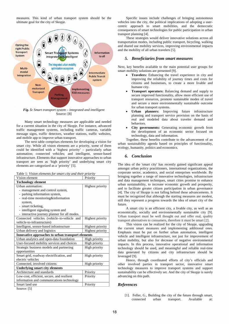
measures. This kind of urban transport system should be the ultimate goal for the city of Skopje.
Fig. 5: Smart transport system – integrated and intelligent
Source: [8]
Many smart technology measures are applicable and needed for a current situation in the city of Skopje. For instance, advanced traffic management systems, including traffic cameras, variable message signs, traffic detectors, weather stations, traffic websites, and mobile app to improve urban transport.
The next table comprises elements for developing a vision for smart city. While all vision elements are a priority, some of them could be identified with a ‘highest priority’ – particularly urban automation; connected vehicles; and intelligent, sensor-based infrastructure. Elements that support innovative approaches to urban transport are seen as ‘high priority’ and underlying smart city elements are categorized as a ‘priority’ [5]. Table 1: Vision elements for smart city and their priority Vision element Priority Technology element Urban automation:
- management and control system, - parking information system, - real-time monitoring&information
system, - smart ticketing, - intelligent signaling system and - interactive journey planner for all modes.
Highest priority
Connected vehicles (vehicle–to-vehicle and vehicle-to-infrastructure)
Highest priority
Intelligent, sensor-based infrastructure Highest priority Urban delivery and logistics Highest priority Innovative approaches to urban transport elements Urban analytics and open-data foundation High priority User-focused mobility services and choices High priority Strategic business models and partnering opportunities
High priority
Smart grid, roadway electrification, and electric vehicles
High priority
Connected, involved citizens High priority Underlying smart city elements Architecture and standards Priority Low-cost, efficient, secure, and resilient information and communications technology
Priority
Smart land use Priority Source: [5]
Specific issues include challenges of bringing autonomous vehicles into the city, the political implications of adopting a user-centric approach to smart mobilities, and the democratic consequences of smart technologies for public participation in urban transport planning [4].
These strategies would deliver innovative solutions across all transportation modes, including public transport, bicycling, walking and shared use mobility services, improving environmental impacts and the mobility of all urban travelers [5].
5. Beneficiaries from smart measures Next, key benefits available to the main potential user groups for smart mobility solutions are presented [9].
• Travelers: Enhancing the travel experience in city and improving the reliability of journey times and costs for citizens and businesses, to create a more livable and humane city.
• Transport operators: Balancing demand and supply to secure improved functionality, allow more efficient use of transport resources, promote sustainable modes of travel and secure a more environmentally sustainable outcome for urban transport systems.
• Urban planners: Improving future infrastructure planning and transport service provision on the basis of real and modeled data about traveler demand and behaviors.
• City governments: Generating economic growth from the development of an economic sector focused on technology, data and information.
Together, these benefits contribute to the advancement of an urban sustainability agenda based on principles of functionality, ecology, humanity, politics and economics.
6. Conclusion The idea of the 'smart city' has recently gained significant appeal amongst urban policy practitioners, international organizations, the corporate sector, academics, and social enterprises worldwide. By bringing together a range of innovative technologies, infrastructure and data management techniques, smart cities promise to enhance urban sustainability, to increase economic growth and prosperity, and to facilitate greater citizen participation in urban governance [4]. The city of Skopje is not falling behind these advancements. It must be recognized that although the starting measures are modest, still they represent a progress towards the idea of smart city of the future.
A smart city is an efficient city, a livable city, as well as an economically, socially and environmentally sustainable city [9]. Urban transport must be well thought out and offer real, quality transport alternatives to consumers, therefore it must be smart [2].
This vision can be realized for the city of Skopje, upgrading the current smart measures and implementing additional ones. Emphasis must be put on further urban automation, intelligent vehicle and intelligent infrastructure, not just for improvement of urban mobility, but also for decrease of negative environmental impacts. In this process, innovative operational and information technology should be used, and meaningful and reliable real-time data generated by citizens and city infrastructure should be leveraged [9].
Hence, through coordinated efforts of city’s officials and other involved parties in transport sector, innovative smart technology measures to improve transport systems and support sustainability can be effectively set. And the city of Skopje is surely advancing on this path. References
[1]. Feller, G., Building the city of the future through smart, connected urban transport. Available at:
18

http://thecityfix.com/blog/building-city-future-smart-connected-urban-transport-integrated-communication-efficiency-meeting-minds-gordon-feller/.
[2]. Kunieda, M., Gauthier, A., Gender and urban transport: smart and affordable, Module 7a – Sustainable transport: A sourcebook for policy makers in developing cities, Deutsche Gesellschaft für Technische Zusammenarbeit (GTZ) GmbH, Eschborn, Germany, 2007, p. 50.
[3]. Rosenberg, S., Sustainable urban transportation: Smart city driving. Available at: http://cityminded.org/sustainable-urban-transportation-smart-city-driving-8392.
[4]. Urban mobilities in the smart city. TSU Seminar series, 2016. Available at: http://www.tsu.ox.ac.uk/events/ht16_seminars/
[5]. Questions and answers for the beyond traffic smart city challenge. Available at: https://www.transportation.gov/smartcity/q-and-a
[6]. www.skopska.mk
[7]. http://www.jsp.com.mk/proekt.aspx?proekt=20
[8]. Role of urban transport in smart cities, Urban mass transit Company limited, Roundtable discussion, Urban mobility India, November 2014.
[9]. Urban mobility in the smart city age, Smart cities cornerstone series, Schneider electric, ARUP the Climate group. p. 44.
19

PROGRAMMING MODULE DESIGN FOR SETTING TECHNOLOGICAL PARAMETERS FOR WORKPIECES
Eng. Matsinski P., MA, Assoc. Prof. Eng. Topalova M., PhD, Assoc. Prof. Eng. Tsekov L., PhD Technical University of Sofia, Engineering and Pedagogical Faculty of Sliven, Bulgaria
[email protected], [email protected], [email protected]
Abstract: This paper presents an option of formalizing input data in automated design processes for machining. A tabular data model required by the technology technician is designed to develop products for the machining process, namely a workpiece. A script-based approach of human-computer dialogue in the setup of structural and technology parameters of a workpiece is adopted as well as particular algorithms to be submitted into the system.
Keywords: SYSTEM ANALYSIS, COMPUTER AIDED PROCESS PLANNING, TABULAR DATA MODELLING, STRUCTURAL PARAMETERS, LIFECYCLE, LOGIC CONTROL
1. Introduction Technology Design (DT) process is an idealised creative
process of the human brain based on a priori information from the structural design of each item and a posteriori data, providing particular production. This determines the complexity of input data into Computer aided process planning (CAPP) systems containing both output results of structural design and basic data for resource provision of production processes. Practically, formalization of the inputs in CAPP systems and development of an efficient database (DB) schema are the main factors that ensure high quality and efficiency in managing the technology design process and the new product development.
In order to fulfill the task the following terms and clarifications have been adopted, specified in the basic concepts and related to technological design:
• Subject of our scientific research is a machine-building product, namely a workpiece, resulting from machining.
• Objective of technology design is to develop and maintain effectiveness of the product across all phases of its lifecycle from planning, analysis, design and implementation through continuous monitoring and optimization of each intermediate stage.
• Development of algorithms aims at human-computer dialogue, which is a proper combination of user-guided dialogue, system-guided dialogue and scenario-based design.
• Data is entered and selected from tables, being verified by continuous visual, and where possible mathematical and logical control.
• Entry algorithms follow the already chosen approach [4] of maximum unification and modular implementation ensuring updating.
2. Tabular Input Data Model A source of basic inputs for CAPP system is the structural
design results, derived by different means and supplemented with mandatory production and operational requirements for each particular product. Data related to supply (stock of resources, raw materials, etc.), staff (labour force, labour productivity, etc.), distribution (feasibility, cost, etc.) plays an essential role. Marketing data connected with the characteristics and prospects of every detail in the functional and structural analysis of the product at all stages of its lifecycle is also of great significance.
The perspective adopted here regards formalization of input data into technology design process as classification structure represented by functional modules in technological database (TDB):
• Data reference for the workpiece: drawing number, shape, dimensions, material, weight, accuracy, manufacturing program, etc. (Table 1);
• Billet condition data: type, shape, dimensions, etc. (Table 2);
• Additional data requirements: type of product, system, functional, structural requirements, etc. (Table 3).
Table 1: Structural inputs for the workpiece
Table 2: Billet condition data
Table 3: Additional requirements for the product
It is essential for the input stage to ensure authenticity of the inputs, their accuracy and completeness across all stages of the lifecycle. Thus, two main types of data are involved, namely mandatory and recommended.
To determine mandatory data, it requires both a comprehensive systematic analysis of the information flow and definition of the necessary and sufficient conditions for managing all stages of work preparation.
Recommended data should be of the sort that the system analyst, designer and CAD technician could miss to submit, without consequences to incorrect implementation of design and planning processes.
The diversity in the type and application of the inputs in the TDB tables has to be organized into groups of products and of workpiece structure.
For instance, the structural input table, apart from the serial product numbers, includes the following groups:
• General data: drawing number, name and shape of the workpiece;
• Dimensions: maximum linear and angular dimensions of the workpiece;
• Material: type and brand name material selected by the designer;
• Workpiece weight; • Accuracy and precision: required level of accuracy of
linear measurements and angular measurements, accuracy of shape, position and orientation accuracy, beating and surface roughness.
• Additional prescriptions: requirements for hardness, additional treatments to achieve it, coating, etc.
• Production program: annual program for the production of the workpiece, batch size, etc. [1, 2, 3].
General Data
Dimen-sions
Mate- rial Weight Accuracy
Indicators Additional
Prescriptions Production Program
General Data
Dimen- sions
Mate- rial Weight Accuracy
Indicators Surface
Roughness
Additional Prescrip-
tions
General Data
Information System
Requirements
Functional Requirements
Structural Requirements
Performance Requirements
20

Mandatory data can include dimensions of the workpieces, such as length and diameter for rotational symmetrical workpieces; length, width and height for prismatic workpieces and so on.
Incomplete data dimensions are a prerequisite for the uncertainty of the type and dimensions of the working area of the machine and the impossibility of applying design technology, respectively.
Billet condition data is grouped in the same way as described above concerning structural input data for workpieces. The difference is in the parameters reflecting surface quality: depth of the surface deformed layer, spatial variation and relative workpiece distortion.
3. Algorithms and software to setup structural and technological parameters of workpieces
Due to the large number of structural and technological parameters of the workpieces and their complex interrelationships the task of formalizing input data needs to be decomposed into multiple subtasks so as to create a hierarchy. This suggests implementation of decision on a modular basis as each module performs a particular subtask and represents a relatively autonomous decision.
3.1. General framework for algorithms to setup structural and technological parameters of workpiece (Figure 1)
In automated design processes for machining there are two main options for entering structural and technological parameters of the workpiece: manual – from pen or pencil drawings and automated – from CAD systems. Setting parameters for workpieces from CAD systems can be done in two ways by means of reading data from the CAD model, which has been recorded in a neutral file format
(STEP, DXF, etc.) or as a result of exchange of information between graphics rendering and CAD systems. In the last two cases the CAPP system must include a module for unified access, obtaining and control of input data by the design technician.
The dialogue requires an appropriate entry methodology as the result determines system’s mode of operation: manual or automated. If submitting data is manually selected, human-computer interaction (HCI) follows the user-guided model. In the automatic mode, task execution continues with the inclusion of a special module for obtaining data from CAD systems. Taking into consideration the wide variety of CAD systems and especially data completeness at data set level, the algorithm provides for mixed mode of data submission. It is realized by checks for input completeness and/or for data obtained by returning execution to General Data Entry Block for the workpiece.
Control is both logical and visual and in the absence of mandatory values for structural parameters of the workpiece the cycle of iterations closes for entering missing data. Cycle exit and data record in Structural Parameters Database (Table 1) occur when all required mandatory parameters have been entered.
The process of finishing condition data submission takes place in a similar way, however under complete supervision: visual, mathematical and logical.
Additional prescriptions are entered directly by the technologist and are visually controlled while the process of TD is repeated and indirectly controlled so it frequently involves multiple-criteria optimization. The nature of information in this table is often subjected to entering catalog data from reference tables stored in system libraries in CAPP system.
Figure 1. General framework for algorithms to setup structural and technological parameters of workpieces
3.2. Algorithm for accuracy indicators entry (Figure 2) Normative documents (standards, norms, etc.) determine different ways to refer to accuracy indicators in design documentation. For example, the lack of a prescription for a minimum tolerance of linear measurements in drawings does not mean there have not been any intentions to do so. This calls for the design of CAPP system be defined a function with prescribed tolerance in accordance with the normalized by the designer maximum degree of accuracy.
In non-machine technology design it is the technician who does this prescription in the design process. Therefore, accuracy parameters entry begins with initializing made by the designer prescriptions. The step is significant for user-guided dialogue in submitting each of the indicators. The dialogue is mixed, providing full control of input (visual, logical and mathematical).
The complicated relationship between accuracy indicators requires mathematical, logical and other data processing from libraries in CAPP system. Therefore, the algorithm for accuracy parameters entry is based on modular approach. The algorithm structure is divided into fundamentally identical groups of blocks for various accuracy indicators. Indicators entry takes place consecutively, starting with possible tolerances for linear dimensions. Using control prescription and visualization help limit deviations in the absence of data from this structural design. Similarly, if there is lack of evidence of deviations from angular dimensions, values according to the ones normalized by the designer for maximum accuracy are assigned. Entering each of the following indicators for form accuracy, precision orientation and location as well as beating is carried out in case there is data for each one in the design documentation. Visual control and/or control with mathematical and logical relationships is realized between inputs and values of linear dimensions. Entering prescriptions for
21

surface roughness and tolerances for linear and angular dimensions is managed by an interim control for entering values based on normalized by the designer maximum roughness.
4. Conclusion The proposed table model is based on the formalization of input
data and provides systematic approach to technology design.
The developed algorithms define human-computer dialogue by means of visual, logical and mathematical control so as to achieve authenticity, accuracy and completeness of the process for entry input of the workpiece and the billet.
Figure 2. A node-positioning algorithm of accuracy indicators entry
5. References 1. Диков А. Технология на машиностроенето, С., Софттрейд, 2006, p. 323 // ISBN-10: 954-334-034-X.
2. Клепиков В. В., А. Н. Бодров. Технология машиностроения, М., Форум, 2008, p. 864 // ISBN 978-5-91134-251-7.
3. Пучков А. А., А. В. Петухов. Основы технологии машиностроения. Учебное пособие, Гомель, 2012, p. 276.
4. Цеков Л., М. Топалова, Пл. Мъцински. Таблично моделиране на технологични процеси в машиностроенето. Машиностроене и машинознание, year IX, is. 2, ТУ – Варна, 2014, pp. 30-33 // ISSN 1312-8612.
Acknowledgements The presented paper is funded by the Scientific and Research Centre of Technical University of Sofia, Contract № 152PD 0029-16/2015.
22

TECHNOLOGICAL SUPPORT OF PERFORMANCE CHARACTERISTICS OF MACHINE COMPONENTS
ТЕХНОЛОГИЧЕСКОЕ ОБЕСПЕЧЕНИЕ ЭКСПЛУАТАЦИОННЫХ СВОЙСТВ ДЕТАЛЕЙ МАШИН
D. Sc. in Engineering V. F. Bezjazychnyi,
P. A. Rybinsk State Aviation Technical University, Russia, Rybinsk, Pushkin str., 53 E-mail: [email protected]
The relationship between the layer quality parameters of the machined surface and the technolog-
ical conditions of cutting has been presented, as well as the calculative estimation of the performance characteristics of machine components: fatigue life, wear life, and compression joints' strength.
KEYWORDS: CUTTING CONDITIONS, PROPERTIES OF MATERIALS OF MACHINE COMPONENTS, QUALITY OF THE SURFACE LAYER, PERFORMANCE CHARACTERISTICS.
1. Introduction.
Managing the surface layer quality in order to provide the performance characteristics for machine components makes feasible calculating correlations between the parameters which characterize the surface layer quality and the cutting conditions. In this regard, the functional relation has been defined between the cutting condi-
tions, the tool geometry and the surface layer quality parameters as well as the cutting accuracy based on the properties of the machined and the tool materials and the stiffness of the machine-attachment-tool-work piece technological system:
( ) ост н p т д р д и ст д р
пл 1 1 сист 1 1 р 1 р
, , , , , , , , , , , , , ,, , , , ,
, , α , , , , , , ,.
h Rz T E аt S v r f
с , , , j В Н L Hσ σ τ µ β β λ λ λ
ϕ = ρ θ γ ϕ ρ α α
where Тр is the size tolerance provided when cutting; βд and βи are the coefficients of the linear expansion of the machined and the tool materials; Ед and τp are the elasticity modulus and the flow shear strength of the machined material, respectively; λд and λp are the heat conductivity coefficients of the machined and the tool materi-als; θпл is the melting point of the machined material; α and γ are the face and the end tool edge angles; ϕ and ϕ1 are the main and the auxiliary cutting edge angles in the plane; ρ1 is the rounded cutting edge radius; В1 and Н1 are the width and the height of the tool hold-er cross section; Lр is the length of the cutter part projecting from the tool head; Н is the size of the work piece; λст is the heat conduc-tivity of the cutter holder material; α1 and αр are the conductivity coefficients of the machined material and cutter holder material; jсист is the stiffness of the machine-attachment-tool-work piece sys-tem; cρ is the volumetric specific heat of the machined material; S is the feed (the tool displacement rate); t and v are the cutting depth and rate; r is the tip radius in the plane; σост is the value of residual stresses on the set level from the work piece surface; hн is the de-gree of cold working of the surface layer material; Rz is the peak-to-valley deviation on the work piece surface; δ is the wear flat height
on the tool point back face; а is the thermal diffusivity of the ma-chined material; σТ is the tensile yield strength of the work piece material.
Thus, the cutting conditions and the tool geometry are the function of the characteristics of the work piece surface layer, cut-ting accuracy, properties of the machined and the tool materials, work piece and the cutter dimensions, rigidity of the technological system.
2. Findings of the study.
To manage forming the work piece surface layer the cal-culative dependencies were obtained to define residual stresses in the surface layer σост, those of degree N and depth hн of cold work-ing, and parameters of surface roughness Rz etc. Some examples are given below.
For instance, axial residual stresses σо.ост in the surface layer caused by the thermal effect, at r > rон and σо.о max < 2σт are determined by the following formula:
[ ]
[ ],
1)(2
1
)(1
)(2 д1д
21вн
21
2
11вн
11
2
1н
2в
2н11
1н
то.ост
22
22
2
2
µ−β
+−−+
−
−+−−++
−+
+−+
+σ−=σ
++
++
ЕА
arraX
arraXar
rraaarr
XX
XX
X
X
where r is the work piece radius from the center in which the values of the residual stresses are determined; rн and rв are the outer and the inner radii of the work piece; µ is the Poisson's ratio of the work
piece material; А1 and Х2 are the values defined by the technological cutting conditions [1].
23

44
3
1 021,0042,005,0
1
101 sinsin)( XX
dXX
A аБВCA −−
−
γα
ρθ= ,
where 1Б aaν
= is the cutting process dimensionless group charac-
terizing the impact of cutting conditions on the temperature in the surface layer comparing to the impact of heat-transfer properties of
the machined material [2]; 1tg 1
B =β
is the dimensionless group
characterizing the plastic yield degree of the removed stock material and the material of the work piece surface layer; β1 is the relative
shear plane inclination; С0, Х1, Х3, Х4 and d are the values depend-ing on the cutting conditions [1].
The depth of cold working in the surface layer is deter-mined based on the condition of equality:
σу + σн = – σт ,
where σу is the stress conditioned by the force impact on the surface layer; σн are the stresses caused by the heat impact on the surface layer.
211
p
1
рy 1
1;;;cos2
;;2 µ−
⋅
γ
∆∆
απ
τ−
ψ⋅
π
τ=σ B
hyE
bb
ah
hyВ ;
( )
×−
++−−µ−
β=σ
д2
в2
он1н
1
д1дн )(5,0
1)1(
2
2 Errarr
аЕА Х
Х
×+−+
++
−+
+−+−× ++ 22 1
1вн2
1н
2
1онн11оннд )(
12)( ХХ arr
Хar
ХarrarrE
, )(5,0
212
он2
н1д
т1д
2
1вн
2
1н2
−β
σ−
+
+−−
++
× rrА
aEХ
arrХar Х
where τр is the flow shear strength of the machined material; h, ∆, ∆1 are the dimensions of the area of the plastic material in the sur-face layer; у is the depth of the layer under consideration from the surface; rон is the radius corresponding to the boundary of elastic and plastic flow in the surface layer under heating, rон = rн – r = у.
The degree of the cold working on the work piece surface is defined by the formula:
( )н
0,8в вэ
,1,25 /
hN =σ σ
where σв is the yield value of the machined material; σвэ is the yield value of the electrical steel taken as a standard.
If the cutting rate changes in dependence of the speed of the maximal build-up forming νнар to the optimal νо, then at
( ) ( )21 1 2 1 cosr S r t r − − ≤ ≤ − ϕ the peak-to-valley ratio is as
follows, mm:
( )
[ ]( )( )
( )
( )
2
1
sin112
sin12
1p
075,01
57,01p
3,0345,01
57,0115,0
165,0
43,01,01
7,01
125,01
p
cos
sincossin
1arccos5,0
6625,0vsin85,2
sinvarctgtg11
1
81
2
2
α×
ρδ+
γ+γα+
+−ρτ−
−ρβελ+λα×
×
αλρθρ
γ−++τ
=
−
−
γ−−
γ−−
BBa
Bab
aba
acba
BB
t
rRz
xb
xb
.
Using the above dependencies to determine the surface layer quality parameters the dependences were obtained to define the indices of performance characteristics of machine components. So, the endurance limit of the work piece material machined with the edge tool is determined as follows:
– when turning
( ) 09,0ост
147,0н
05,0вэв1
−−− σ⋅⋅⋅σσ⋅=σ hRzm K ;
– when milling
( ) 063,0ост
139,0н
067,0вэв1
−−− σ⋅⋅⋅σσ⋅=σ hRzn L ,
where m, n, K, L are the values depending on the cutting type [1]; σв
and σвэ is the ration between the yield value of the machined mate-rial and the yield value of the electrical steel taken as a standard.
The wear rate of the machined surface is defined by the formula:
24

( )
( )
( )( ) ( ) .
μ164,341
γsin45,01ρ
vsinτ
ρβελλsin3,4
ρ6625,0
81
7,30316,0
1323,084,0161,0216,0161,01323,0
м
0
2,512,0719,0
12
1,01
04,0
74,00
25,00
05,043,0p
075,01
57,0p
3,0345,0
157,0115,0
0125,0
1
5,02
1
0
0
0
+ν−+−++ν−
++ν−
−
−
−−
+ν
−
σ+ν
−×
×α
+
αν
×
×θ
×
×α⋅=
yyy
y
ttt
t
EAN
kf
b
mcta
amta
ca
r
bJ
c
n
n
n
h
,
where Rz is the peak-to-valley ratio of the contact surface profile, mm; ν and b are the bearing surface approximation curve parame-ters; σ0 is the acting stress in the contact area of mating surfaces, МPа; N is the load acting on the contact, Н; Ас is the nominal area outlined by the dimensions of the adjoining solids, mm2; µ is the Poisson's ratio of the work piece material; Е is the elasticity modu-lus of the material which wears out faster, Pа; ty is the friction fa-tigue curve parameter [3]; K is the coefficient characterizing the stress condition on the contact (for brittle materials K = 5, for high-plasticity materials K = 3); fм is the value of the molecule-based component of the friction ratio.
Thus, the surface wear rate is the function of its cutting conditions, as well as the properties of the work piece material.
When making pressure couplings the values of axial force Ро and torque Мкр, which provide the strength of such connections, are determined by the formulas:
- when manufacturing joinable parts made of the same material:
( ) ( )
( ) ( ) ,2,11
,2,112
22
2221
11
21н2
22,0
кркр
22
2221
11
21н2
22,0
oco
NWC
NWC
RzRzfldM
NWC
NWC
RzRzflP
+
+−δ⋅
α
σ⋅µ+⋅⋅⋅⋅π=
+
+−δ⋅
α
σ⋅µ+⋅⋅⋅π=
where l is the length of the contact area of the mating parts; d is the nominal mating diameter; fос and fкр are the friction coefficients
under the press fitting and press fitting with twisting; δ is the value of the nominal tension; Rz1 and Rz2 is the peak-to-valley ratio on the contacting surfaces; N1 and N2 are the cold working degrees on the surface of mating parts; 2,0σ′ and 2,0σ ′′ are the conventional yield
stress for the materials of the mating parts; W1 and W2 are the values of the stored power in the surface layer of the materials of the first and the second mating parts; µ1 and µ2 are the Poisson's ratio of the mating part materials [3]; С1 and С2 are the factors depending on the part dimensions and the Poisson's ratios of the materials of the mating parts.
3. Conclusion.
Thus, the methods was presented to calculate the cutting mode, providing the predetermined performance characteristics of work pieces and allowing to control the cutting process thereby ensuring manufacture of reliable and durable products and making the manufacturing process be science-intensive and cost-effective.
4. References.
1. Bezjazychnyi V.F. The method of similarity in engineer-ing technology. – M: Machinostroyeniye, 2012. – 320 p.
2. Silin S.S. The method of similarity when cutting materi-als. – M: Machinostroyeniye, 1979. – 152 p.
3. Malinin N.N. Applied theory of plasticity and creep – M: Machinostroyeniye, 1970. – 400 p.
25

COLD DRAWING OF PURE MAGNESIUM WIRE
Haruka Takeura1. Kazunari.Yoshida2.
1Dept. of Graduate Student, Tokai University 4-1-1 Kitakaname, Hiratsuka, Kanagawa, Japan
2Dept. of Precision Engineering, School of Engineering, Tokai University
Corresponding author. E-mail: [email protected]
Abstract:
Pure magnesium is a material with very high functionality, however, the cold drawing of this material is very difficult, because it has a
hexagonal crystal structure and until this day there is no optimal cold wire drawing conditions. In this research, the goal is to create the optimal
cold drawing conditions for pure magnesium wires. The first step is the investigation of the annealing temperatures by using tensile testing of
the annealed wires, which will allow is to optimize the manufacturing of magnesium. Following the results listed below, the most suitable
annealing temperature was 250°C for a reduction of 10% per pass. After the reaching the drawing limit and examining the drawn wires, cracks
in the center of the wires, that is why suppressing their occurrence by applying a middle annealing to the process is needed. Consequently, it
is possible to produce a cold fine drawn pure magnesium wire, without cracks or defects on the surface or hindering its medical properties.
Keywords: PURE MAGNESIUM, COLD WIRE DRAWING, ANNERLING, DIAMOND DIE
1. Introduction
Magnesium is a very light high functionality material that has high
vibration absorbency, heat dissipation, electromagnetic wave-
shielding and recycling efficiency. However proper cold wire
drawing conditions haven’t been establish, that is why warm or hot
processing is commonly used. As a result, strength improvement of
the wires is not possible, that is why the production of medical tools
is disregarded. If it were possible to cold draw magnesium wires, the
applications for material products would expand.
In this research, an investigation regarding the optimal cold drawing
conditions of pure magnesium wire, the changes in the mechanical
properties of the material after drawing and the problems that might
occur during processing is conducted, the aim of which is to produce
pure magnesium wire.
2. Preconditions and means for resolving the
problem
2. 1. Tested wire and annealing conditions
Table1 shows the sample material and the annealing condition.
2. 2. Wire drawing process
In this research, the used material is pure magnesium wire with a
diameter of 2.58mm. It was subjected to wire drawing with a
reduction per pass (R/P) of 10%, 15% and 20%. The wire drawing
process is explained in Fig. 1 and equations (1), (2). The drawing
speed used was 300 mm/min, the drawing dies were tungsten carbide
dies and diamond dies with a half-angle of 6 degree and for the wire
drawing process teflon resin lubricant AGP8H and Na-soap powder
were used.
3. Solution of the examined problem
In order, the present goal to be achieved, narrowing down the
optimum drawing conditions for drawing of pure magnesium wires
was needed. The low formability of pure magnesium prevents it from
having a high drawing limit, following this, the improvement of the
drawing limit can be achieved with proper annealing of the wires
before and during the wire drawing processing, for that purpose the
annealing conditions that were examined were 200°C, 250°C and
Tested material Pure magnesium
Diameter [mm] 2.58
Annealing
conditions
300°C ,250°C ,200°C
keep 1 hour
D0 D1, Dn
Direction
α°
Fig.1 Definition of pass reduction and total reduction
in wire drawing
𝑅/𝑃 = 1 − 𝐷1
𝐷0 2 × 100 % …(1)
𝑅𝑡 = 1 −
𝐷𝑛
𝐷0 2 × 100 % …(2)
Table1 Tested material and annealing condition
26

300 °C. The second thing that needed optimization was the reduction
per pass, the following R/P were suggested for this experiment 10%,
15% and 20%. Finally, the last thing that needed confirmation was
the material of the drawing dies, in this case the tested dies were
tungsten carbide die and poly-crystal diamond die.
After comparing the different wire drawing conditions, an optimum
drawing method was chosen and used in order to fabricate wires for
medical tests.
4. Results and discussion
4. 1. Tensile test of the annealed pure magnesium wires
Firstly, tensile test was performed on the drawn pure magnesium
wires, in order to investigate their mechanical properties, following
this a Stress-Strain curve was build using the results. The Stress-
Strain curves can be seen in Fig. 2.
The highest tensile strength exhibited by the drawn wires was of
208.2MPa for the annealed wire at 200°C, compared to the 250°C
with 187.6Mpa and 300°C with 186.8Mpa, but the elongation at
fracture for that wire was only 3.87%, which is almost three times
smaller than 11.5%(250°C) and 11.2%(300°C).
In the drawing processing, high ductility materials are more suitable
for drawing than more brittle materials, following the results shown
in Fig. 2, the most suitable annealing temperature for the drawing of
pure magnesium wires is 250°C, based on the high elongation in
tensile test.
In the SEM (Scanning Electron Microscope) image of the break side
of the annealed wire, it can be seen that the 200°C and 300°C has a
relatively brittle surface, compared to the 250°C wire, which has
dimple fracture surface. It can be concluded that by using the 250°C
annealing temperature, a high ductility material can be achieved.
4. 2. Changes of the drawing limit a wire with different
annealing temperatures
In order to investigate the drawing limit of the pure magnesium, each
of the annealed wires were used with the three different R/P and were
drawn using tungsten carbide dies. The results are shown in Fig. 4.
After drawing of all annealed wires, the wires that used 10% R/P were
able to be drawn up to the goal of Rt=68.8%. For the 20% R/P the
200°C, 250°C and 300°C were drawn up to Rt=47.5% for 200°C and
Rt=57.1% for 250°C and 300°C, but in the case of 300°C there was
a breaking that occurred at the 47.5%, as the 250°C were successfully
drawn until 57.1%. Finally for R/P of 15%, only the annealed wire at
200°C broke at Rt=56.1%, as the 250°C and 300°C were able to be
drawn up to the drawing limit of Rt=68.8%, but in the 300°C’s case
two breaks occurred at the finishing diameter, but 250°C’s case only
one of the samples broke.
4. 3. Internal defect which is occurred in drawn wire
After drawing the pure magnesium wires while using the optimum
drawing conditions that were chosen after the previous experiments
– annealing temperature of 250°C, R/P=10%, , it was discovered that
internal defect in the center of the wire occurred, as seen in Fig. 5.
200
150
100
50
0 0 0.05 0.15 0.1 0.2
250
Str
ess
σ [
MP
a]
Strain ε
200℃
300℃
250℃
Fig.2 Stress-Strain curve of magnesium wire in tensile test
200℃ 250℃
300℃
Fig.3 SEM image of magnesium wire surface after tensile test
68.8 65.3 61.5 57.1 52.4 47.5 41.1 34.4 27.3 19.0 10.0
200℃ 250℃ 300℃ R/P=10% R/P=20%
To
tal
red
uct
ion R
t [%
]
R/P=15% Fig.4 Drawing limits of magnesium wire
a) b) c)
Break
Drawn
27

Due to the occurrence of internal defect, cupping in the wire, it
becomes unfit to be used as a production material.
In Fig. 6 it is shown that the couse of inner cracks is due to the tensile
stress in the center part of the wire. It is possible to suppress its
occurrence by lowering the half-width of the die or it increasing the
reduction per pass, because by the reduction of the friction force is
necessary. Based on the graph in this Fig. 6, it was determined that
any higher angle than 6º was unsuitable, also to further decrease
friction diamond dies were suggested for this experiment.
4. 4. Drawing process using a diamond dies
pass Tungsten carbide dies
[MPa]
Diamond dies
[MPa]
Difference
[%]
1 55 48 12.7
3 66 62 6.1
5 70 67 4.3
In Table 2, the drawing stress using tungsten carbide and diamond
dies, for reduction of 10% can be seen, the diamond dies had a lower
drawing stress of about 7-8%. After drawing the pure magnesium
wires annealed at 200°C, 250°C and 300°C while using R/P of 10%,
reaching the drawing limit of Rt=68.8% was possible for all wires,
that is why in order to compare the increase of drawing limit and
decrease of drawing stress by using diamond dies, the R/P used was
20% to establish the effectiveness of using diamond dies In this case,
the results can be seen in Fig. 7.
Furthermore, after drawing the wire to Rt=68.8% with a R/P=10%
and annealing temperature of 300°C, the finishing wires were
examined by using SEM, in order to observe the difference between
the drawn wires’ surfaces between the tungsten carbide and diamond
dies. The results can be seen in Fig. 8.
There are many defects on the surface of the tungsten carbide die
drawn wire, such as surface flaw and die marks, after reaching the
drawing goal, but in the case of the diamond die, after drawing it
exhibits much finer surface compared to the tungsten carbide die and
a lack of die marks.
Following this, it can be concluded that the diamond dies present
much better effectiveness for drawing of pure magnesium wires, with
higher drawing limit, lower drawing stress and a finer surface of the
finishing drawn wire, but even after the application of diamond dies,
the occurrence of cupping still persisted, which led to the introduction
65.3
61.5
57.1
52.4
47.5
41.1 34.4
27.3
19.0
10.0
200℃ 300℃
To
tal
red
uct
ion [
%]
Tungsten carbide dies Diamond dies
Fig.7 Drawing limits of magnesium by using a diamond dies
(α=6 º, R/P=20%)
Fig.5 Internal defect in drawn wire
(α=6°, R/P=10%, 𝑅𝑡=68.8%)
300μm
stress
die
Tensile
Direction
Danger
40
30
20
10
0 5 10 15 20
R/P
[%]
α [°]
Fig.6 Occurrence of cupping in the wire1)
Safe for internal defect
Table 2 Difference in drawing stress
between tungsten carbide dies and diamond dies
Break
Dia
mo
nd
die
s W
C d
ies
500μm 100μm
Fig.8 SEM image of drawn wire surface
with the WC dies and diamond dies (α=6 º, R/P=10%,𝑅𝑡=68.8%)
28

of an intermediate annealing for further increasing the workability of
the material.
4. 5. Effect of the intermediate annealing
The drawing of pure magnesium wires with two intermediate
annealing points (Rt=34.4% and Rt=57.1%) and a single intermediate
annealing point (Rt=34.4%; Rt=41.1%; Rt=47.5%), were examined
for a total reduction of Rt=68.8% and the changes of mechanical
properties were summarized in the stress-strain diagram of Fig. 9.
In the case of single annealing with Rt=41.1%, the elongation at
fracture was about 0.067 and total tensile strength was around
230Mpa. The case of the two intermediate annealing the tensile
strength was higher by comparison with 237Mpa, but the elongation
at fracture was 0.06, which is lower than the single annealed wire at
Rt=41.1%. Also in the case of all other annealed wires, the tensile
strength of the drawn finishing wire was close to the previously
mentioned wires, but the elongation at fracture was much lower.
Following these results, the annealing most suitable for this wire
drawing, is the single annealing at Rt=41.1%
In addition, it the inner section of the drawn wires were checked to
confirm the presence of defects in the center of the drawn wires. In
Fig. 10, the comparison between intermediate annealing of Rt=41.1%
and Rt=47.5%.
After observing the wire drawn with an intermediate annealing with
Rt=47.5%, it was determined that just like the case of Fig. 5, it
exhibits cupping in the center of the wire, rendering it unsuitable for
production of medical tool. In the case of the Rt=41.1%, after closely
examining the center of the drawn wire along its length, no trace of
cupping was spotted. Based on this, it was concluded that by using
intermediate annealing of Rt=41.1% for cold drawing of pure
magnesium with a total reduction of Rt=68.8%, the occurrence of
cupping can be prevented, leading to a more suitable material for the
needed purposes.
5. Conclusion
For the wire drawing of pure magnesium, the most suitable
annealing temperature was decided at 250 ° C, and very effective
means is using a diamond die, also by using a diamond die, a
reduction per pass of 10% and by performing an intermediate
annealing at a cross-section reduction rate of 40%, it was possible to
achieve a diameter of 1.44, without the occurrence of inner cracks in
the center of the wire, which is suitable for the production of medical
tools.
6. Reference
1. Kazunari Yoshida, “My 35 years of research on wiredrawing”,
WIRE JOURNAL INTERNATIONAL, Vol. 44, 2011, 50-56
2. Y. Oishi, K. Mori and N. Kawabe, Sumitomo Electric
Industries,LTD, “Mechanical properties of drawn magnesium
alloy”, proceedings of The Japan Institute of Light Metals, Vol.
108, 2005, 5-6
3. M. Sato, H. Nakamaru and Y. Ri, “High Precision Working of
Aluminum Alloy Tubes by Sinking”, Proceedings of The Japan
Institute of Light Metals, Vol. 95, 1998, 131-132
4. Conruy. J. T “Windows of opportunity for magnesium wrought
products”, Proc. Annu. Meet. Int Magnes. Assoc. Vol. 46, 1989,
53-57
5. O. Hasegawa and H. Nishimura, “Material Characteristics and
Deformation Behavior of AZ31 magnesium Alloy extruded
Tube under Press Bending”, Proceedings of The Japan Institute
of Light Metals, Vol. 99, 2000, 219-220
Two intermediate annealing No annealing
41.1% 47.5% 34.4%
0.08
Fig.9 Stress-Strain curve of intermediate annealed wire (𝑅𝑡=68.8%)
250
200
150
100
50
0
0 0.02 0.04 0.06
Str
ess
σ [
MP
a]
Strain ε
300μm 200μm
Rt=
47
.5%
R
t= 4
1.1
%
Fig.10 The internal defect that occurred to
the annealed drawn wire (𝑅𝑡=68.8%)
29

CoO/Al2O3, CuO/Al2O3 AND NiO/Al2O3 CATALYSTS FOR PHOTODEGRADATION OF MALACHITE GREEN DYE UNDER UV-IRRADIATION
CoO/Al2O3, CuO/Al2O3 И NiO/Al2O3 КАТАЛИЗАТОРИ ЗА ФОТОРАЗГРАЖДАНЕ НА МАЛАХИТОВО
ЗЕЛЕНО БАГРИЛО ПОД УВ ОБЛЪЧВАНЕ
Chief. Assist. Prof. Milenova K. PhD.1, Chief. Assist. Prof. Zaharieva K. PhD.1, Assoc. Prof. Avramova I. PhD.2, Assoc. Prof. Stambolova I. PhD.2, Assoc. Prof. Blaskov V. PhD.2, Assoc. Prof. Dimitrov L. PhD.3, Assoc. Prof. Eliyas A. PhD.1
1Institute of Catalysis, Bulgarian Academy of Sciences, “Acad. G. Bonchev” St., Bl.11, 1113 Sofia, Bulgaria 2Institute of General and Inorganic Chemistry, Bulgarian Academy of Sciences, “Acad. G. Bonchev” St., Bl.11, 1113 Sofia, Bulgaria
3Institute of Mineralogy and Crystallography “Аcad. I. Kostov”, Bulgarian Academy of Sciences, “Acad. G. Bonchev” St., Bl.107, 1113 Sofia, Bulgaria
Abstract: CoO, CuO or NiO supported on Al2O3 photocatalysts were prepared by impregnation and then calcination at 400oC for 3 hours. The obtained samples were physico-chemically studied by Powder X-ray diffraction analysis, X-ray photoelectron spectroscopy and Scanning electron microscopy. The photocatalytic oxidative degradation of aqueous solution of Malachite Green (MG) dye as pollutant using CoO, CuO or NiO supported on Al2O3 under UV irradiation was tested. The results determined that the highest degree of degradation of MG dye after 120 minutes was achieved using NiO/Al2O3 photocatalyst (82%) than that the other materials CuO/Al2O3 (64%), CoO/Al2O3 (59%) and Al2O3 (50%). The calculated apparent rate constants increasing in the order: Al2O3 (2.7x10⁻³ min-1)<CoO/Al2O3 (3.9x10⁻³ min-
1)<CuO/Al2O3 (4.1x10⁻³ min-1)<NiO/Al2O3 (8.4x10⁻³ min-1).
Keywords: NiO, CuO, CoO, Al2O3, MALACHITE GREEN, PHOTOCATALYST, DEGRADATION
1. Introduction Latest industrial development has ameliorated living standards
but due to insufficient environmental monitoring, the continuous discharge of many industrial pollutants (organic compounds derived from synthetic dyes and etc.) is causing major environmental problems. Since these pollutants are carcinogenic at trace levels for aquatic and non-aquatic organisms, a wide range of remediation techniques as: biological, physical, and chemical methods have been applied for water decontamination [1-4]. Photocatalysis is widely used to describe the process based on a series of light-induced redox reactions occurring when a semiconductor (e.g. TiO2, ZnO, SnO2, WO3), interacts with light in order to generate reactive species. This can lead to the photodegradation of the dye pollutants [2]. The challenge for the recent researchers is to create new and effective photocatalysts, applying appropriate synthesis methods by modifying the structure or properties of supports (to achieve more active sites, which may promote the reaction with the reactants) and introduce other elements homogeneously distributed on the support [5]. Non-reactive solid supports such as alumina may significantly control the photochemical reactivity of adsorbed molecules due to electronic interaction between the molecules and the surfaces [6]. The excellent dispersing ability of the alumina surface is much more pronounced in the supported photocatalysts [7]. Al2O3 was used as a catalyst for the photomineralization of hazardous organic molecules [2, 8]. Introduction of some transition metals, such as Cr, V, Fe, Cu, Mn, Co, Ni, Mo etc. may lead to higher catalytic activity [4]. Karunakaran et al. (ref. [6]) concluded that the presence of a semiconductor like (TiO2, ZnO, CuO and other) with Al2O3 (insulator) lead to synergism between them, which improved their photocatalytic performance. The iron oxide supported on alumina was studed in photo-assisted Fenton degradation of different textile dyes [5]. 2-phenyl-4-(1-naphthyl) quinolinium supported on silica–alumina photocatalyst was examined for H2O2 production [9]. The impact of surface of Al2O3/TiO2 [10] and Al2O3–Fe2O3 catalysts [11] on the photodegradation of organic pollutants was discussed in details. Cobalt oxide as photocatalyst was applied for reaction of photocatalytic water-splitting [12]. Cobalt oxide supported on carbon was used for degradation reaction of Methyl Orange [13]. Properties of CuO–CoO/Al2O3 catalysts were investigated for NO reduction by CO [14]. CuO was used as semiconductor photocatalysts for the degradation of dyes [15]. Films of CuO [16] and nickel oxide powders [17] were evaluated as photocatalysts for degradation of Rhodamine B dye. Photocatalytic activity of pure
CuO for H2 evolution reaction was discussed in [18]. Many researchers had anticipated the reaction of CuO on different adsorbents like activated alumina in wastewater treatments [15]. Series of NiO photocatalysts have been investigated in the degradation of Methylene Blue [19].
The present paper deals with synthesis of CoO/Al2O3, CuO/Al2O3 and NiO/Al2O3 powders, prepared by impregnation of previously prepared alumina containing support. They were physicochemically characterized and tested in the photodegradation of Malachite Green dye under UV-irradiation.
2. Experimental 2.1. Synthesis of the samples
The Al2O3 powder was prepared after precipitating aluminium hydroxide. Then it was mixed with bentonite in respect to obtain composite Al2O3: bentonite (90:10) and compressed in tablets. The powder was calcined at 800oC for 8h to obtain γ-Al2O3 (the composite material was synthesized at University of Chemical Technology and Metallurgy, Sofia, with assistance of Assoc. Prof. Nikoleta Kassabova). In order to obtain photocatalytic systems, with active phase NiO, CuO or CoO were used the corresponding water solutions of: Ni(NO3)2.6H2O, Cu(NO3)2.3H2O and Co(NO3)2.6H2O calculated to give 10 wt % content with respect to Ni, Cu or Co amount. The carrier was impregnated with the aqueous nitrate solutions under heating and constant electromagnetic stirring. Than the samples were dried at 100 оС and after that calcined at temperature 400 оС for 3 hours. The prepared photocatalysts was named as: Al2O3 as P1; CoO/Al2O3 as P2; CuO/Al2O3 as P3; NiO/Al2O3 as P4.
2.2. Powder X-ray diffraction analysis (PXRD)
The powder X-ray diffraction patterns were recorded on a Bruker D2 Phaser diffractometer within the range of 2θ values between 5º and 75º using Cu Kα radiation (λ = 0.154056 nm) at 40 kV. The phases were determined by using of JCPDS database (Powder Diffraction Files, Joint Committee on Powder Diffraction Standards, Philadelphia PA, USA, 1997).
30

2.3. Scanning electron microscopy (SEM)
SEM studies were performed on a JSM – 5510 JEOL scanning electron microscope. For morphology observations of the samples the accelerating voltage 10 kV was used.
2.4. X-ray Photoelectron spectroscopy (XPS)
The XPS analyses were performed on a Kratos AXIS Supra with a monochromatic Al X-ray source. Each analysis started with a survey scan from 0 to 1200 eV pass energy of 160 eV at steps of 1 eV with 1 sweep. For the high resolution analysis the number of sweeps was increased, the pass energy was lowered to 20 eV at steps of 100 meV. The X-ray Photoelectron spectroscopy method was used for the investigation of the surface states of Cu;Co;Ni loaded photocatalysts over precursor Al2O3:bentonite. The C1s, O1s, Al2p, Si2p, Co2p, Cu2p as well as Ni2p photoelectron lines were recorded and the obtained spectra were discussed. The surface concentrations of the constituent elements in the investigated catalysts have been calculated, too.
2.5. Photocatalytic investigations
Synthesized samples were investigated for period of 2 hours in the oxidative degradation of Malachite Green (MG) dye in a semi-batch photocatalytic reactor. UV light irradiation was used with power 18 W and мaximal emission at 365 nm. In the beginning of the process the concentration of MG dye solutions was 5 ppm (λmax = 615 nm) accordingly, with catalyst loading 1g/l. Before switching on the UV illumination investigated systems were equilibrated in the dark for about 30 min. All activity tests were run out at a constant stirring rate using continuous air flow at room temperature. To examine the photocatalytic activity of materials, sample aliquots of the suspension have been taken out of the reaction vessel at regular time intervals (powder was separated from the aliquot solution by centrifugation). The absorbance of investigated solutions was measured on UV-1600PC Spectrophotometer (wavelength range from 200 to 800 nm). The degree of degradation is estimated using dependence (C-Co/Co)x100, where Co and C are initial concentration before turning on the illumination and residual concentration of the dye solution after illumination for selected time interval.
3. Results and discussions Figure 1 illustrates Powder X-ray diffraction patterns of the
investigated materials. The presence of γ-Al2O3 (PDF-29-1486), SiO2 (PDF-87-2096) were established in all the samples – P2, P3 and P4. Additionally CuO (PDF-44-0706) for P3 and Co3O4 (PDF-42-1467) for P4 samples are observed in the PXRD spectra.
The Survey spectra are shown in Figure 2 for the illustration of the constituent elements in the catalysts. The position of O1s and Al2p photoelectron peaks at 531.5 eV and 74.5eV, respectively indicate that the support of the studied catalysts is Al2O3. The small quantities of silicon on their surfaces have been detected, also. The binding energy of Si2p peak at around 103.2 eV, is typical for SiO2. This is in coincidence with the XRD results.
The binding energies of Ni2p, Cu2p as well as Co2p photoelectron peaks and the shape of the peaks shows that the loaded elements exist on the surface as oxide, NiO, CuO and CoO as well.
It should be mentioned, that the calculated quantity of Ni, Cu and Co is different and follow the order Cu>Ni>Co although the equal quantity used during the synthesis of the final catalyst.
Figure 3 presents SEM pictures of the three samples: A) P4; B) P3 and C) P2 at two different magnifications (x 1.000 and 8.000).
Fig. 1 PXRD patterns of CoO/Al2O3, CuO/Al2O3 and NiO/Al2O3 photocatalysts.
The SEM observations of NiO supported photocatalyst (Figure 3A) revealed typical layered material. The micrographs presented “plates-like” structures joined in aggregate. In the bigger magnification morphology observations of the sample P4 also demonstrated presence of bulk aggregates with irregular shape and also smaller particles on them.
The SEM images of CuO/Al2O3 (Figure 3B) were consistent from “flake-like” pieces and other bigger particles, with different sizes, and thin ones stuck to their surface. In the bulk and between the different stones were observed fibrous particles. In the larger augmentation it can be seen that the investigated material in some places also revealed porous “spider web-like” structure.
Fig. 2 XPS of NiO/Al2O3, CoO/Al2O3, CuO/Al2O3 samples.
The SEM photographs of CoO/Al2O3 sample (Figure 3C) showed aggregates with almost smooth surface, maybe it was flip off between two grains. It also composed of different little particles like flakes, tiny spots situated on angular species. Some of the broken off pieces had pores. Consequently the pictures also exposed dissimilar pores, according to size, between the particles. On the major magnification common nature of P2 sample displayed that separate grains were sintered.
31

Fig. 3 SEM pictures of samples: A) P4; B) P3 and C) P2 at different magnifications.
Photocatalytic activities of investigated catalysts were tested for
degradation of textile dye Malachite Green under UV-light illumination. The results of dark period before switch on the lamp showed that the absorption capacity of alumina containing support is lower than the supported materials. Absorption increases slightly with adding of active phase CoO, CuO or NiO and it is in the following order: P1<P2<P3<P4 (Figure 4). Figure 4 also represents the degradation degree of the MG dye solution, the supported photocatalysts P2÷P4 showed better extent of degradation of MG dye then the support P1.
Fig. 4 Degradation degree of the MG dye solution under UV-A illumination over investigated samples; where Co is initial concentration of the dye, C is the dye concentration after illumination.
On Figure 5 is shown degree of degradation of P1÷P4 catalysts after 120 min time of illumination, which varied in the range of 59÷82% for impregnated systems and 50% for the support. Among the investigated photocatalysts NiO/Al2O3 showed the highest photocatalytic performance, which is 35% enhancement in comparison to this of Al2O3 sample.
It can be seen from Figure 6 that the reaction course of MG dye degradation as a function of the time of illumination of investigated photocatalysts, follows pseudo first order kinetics. The apparent rate constants k is estimated using logarithmic linear dependence: –ln(C/C0) = k.t. The values of rate constants and degree of
degradation of MG dye for 120 minutes illumination are given in Table 1. Apparent rate constants of supported photo-catalysts were (3.9÷8.4 x10⁻³, min-1), while for the support was (2.7 x10⁻³, min-1). Increasing of absorption was in accordance with enhancement degree of degradation and apparent rate constants.
Fig. 5 Degree of degradation of the MG dye solution after 120 min under UV-A illumination over investigated samples. Table 1: Apparent rate constants and degradation conversion degrees (120min) of investigated photocatalysts regarding MG dye.
Samples k x10-3,min-1 Degradation, %
P4 8.4 82 P3 4.1 64 P2 3.9 59 P1 2.7 50
In our previous work we found out that alumina based samples,
which contain α-Al2O3, ө-Al2O3 and Ca3Al2O6 showed 29% photocatalytic degree of degradation of Reactive Black 5 textile dye and after mechanochemical activation the degree of degradation increased up to 40% [20]. Some researchers reported the existence of unusual synergism when an insulator is present along with a semiconductor like TiO2, ZnO, ZnS, Fe2O3, CdO, CuO and Nb2O5 [6]. Probably, in our case CuO, CoO and NiO supported on γ-Al2O3 composites show synergistic photocatalytic effect and as result of it comes the enhanced dye photodegradation degree.
Fig. 6 Reaction course as a function of the time of illumination –ln (C/C0) of the alumina supported photocatalysts.
In conclusion we can state that all active semiconducting phases (CoO, CuO or NiO) exert considerable catalytic photodegradation
32

of MG dye, whereupon NiO/Al2O3 photocatalyst is superior to the other two systems. In this case both the alumina and the semiconductor particles are likely to be present in the agglomerates. This could lead to the transfer of holes from the illuminated semiconductor to the dye molecule, adsorbed on the Al2O3 surface, resulting in effective separation of the electron-hole pairs and higher rate of photoreaction.
4. Conclusions
The NiO/Al2O3, CuO/Al2O3 and CoO/Al2O3 photocatalytic systems were synthesized by impregnation method. The SEM pictures showed particles and aggregates with sizes around 0.2÷80 µm. The materials were tested as catalysts for photodegradation of toxic pollutant Malachite Green dye under UV light. Photocatalytic degradation of MG dye on Al2O3 samples was 50%. In the case of NiO, CuO and CoO supported Al2O3 photocatalysts the degradation rate increases to some extent due to the synergism between insulating support and semiconducting oxide. The best photocatalytic efficiency was manifested by the NiO supported on γ-Al2O3 (degradation rate 82%), which correlates with its highest adsorption capacity and respectively specific surface area.
Acknowledgements The financial support by National Science Fund, Ministry of Education and Sciences of Bulgaria (Contract DFNI – T-02-16) is acknowledged.
References [1] Asif S. A. B., S. B. Khan, A. M. Asiri. Visible light functioning photocatalyst based on Al2O3 doped Mn3O4 nanomaterial for the degradation of organic toxin. Nanoscale Research Letters, 10, 2015, 355-364.
[2] Rubio-Clemente A., R. A. Torres-Palma, G. A. Peñuela. Removal of polycyclic aromatic hydrocarbons in aqueous environment by chemical treatments: A review. Sci. Total Environ., 478, 2014, 201-225.
[3] Trujillo-Reyes J., J. R. Peralta-Videa, J. L. Gardea-Torresdey. Supported and unsupported nanomaterials for water and soil remediation: Are they a useful solution for worldwide pollution. J. Hazard. Mater., 280, 2014, 487-503.
[4] Fechete I., Y. Wang, J. C. Védrine. The past, present and future of heterogeneous catalysis. Catal. Today, 189, 2012, 2-27.
[5] Soon A. N., B. H. Hameed. Heterogeneous catalytic treatment of synthetic dyes in aqueous media using Fenton and photo-assisted Fenton process. Desalination, 269, 2011, 1-16.
[6] Karunakaran C., R. Dhanalakshmi, P. Gomathisankar. Photomineralization of phenol on Al2O3: synergistic photocatalysis by semiconductors. Res. Chem. Intermed., 36, 2010, 361-371.
[7] Tzirakis M. D., J. Vakros, L. Loukatzikou, V. Amargianitakis, M. Orfanopoulos, C. Kordulis, A. Lycourghiotis. γ-Alumina-supported [60] fullerene catalysts: Synthesis, properties and applications in the photooxidation of alkenes. J. Mol. Catal. Chem., 316, 2010, 65-74.
[8] Tzompantzi F., Y. Pina, A. Mantilla, O. Aguilar-Martínez, F. Galindo-Hernández, X. Bokhimi, A. Barrera. Hydroxylated sol–gel Al2O3 as photocatalyst for the degradation of phenolic compounds in presence of UV light. Catal. Today, 220-222, 2014, 49-55.
[9] Yamada Y., A. Nomura, K. Ohkubo, T. Suenobu, S. Fukuzumi. The long-lived electron transfer state of the 2-phenyl-4-(1-naphthyl) quinolinium ion incorporated into nanosized mesoporous silica–
alumina acting as a robust photocatalyst in water. Chem. Commun., 49, 2013, 5132-5134.
[10] Egerton T. A.. The influence of surface alumina and silica on the photocatalytic degradation of organic pollutants. Catalysts, 3, 2013, 338-362.
[11] Li F. B., X. Z. Li, C. S. Liu, T. X. Liu. Effect of alumina on photocatalytic activity of iron oxides for bisphenol A degradation. J. Hazard. Mater., 149, 2007, 199-207.
[12] Liao L., Q. Zhang, Z. Su, Z. Zhao, Y. Wang, Y. Li, X. Lu, D. Wei, G. Feng, Q. Yu, X. Cai, J. Zhao, Z. Ren, H. Fang, F. Robles-Hernandez, S. Baldelli, J. Bao. Efficient solar water-splitting using a nanocrystalline CoO photocatalyst. Nature Nanotechnology, 2013, www.nature.com/naturenanotechnology,DOI:10.1038/NNANO.2013.272.
[13] Dou J., S. Yin, J. Y. Chong, B. Zhang, J. Han, Y. Huang, R. Xu. Carbon spheres anchored Co3O4 nanoclusters as an efficient catalyst for dye degradation. Appl. Catal. Gen., 513, 2016, 106-115.
[14] Lv Y., L. Liu, H. Zhang, X. Yao, F. Gao, K. Yao, L. Dong, Y. Chen. Investigation of surface synergetic oxygen vacancy in CuO–CoO binary metal oxides supported on γ-Al2O3 for NO removal by CO. J. Colloid Interface Sci., 390, 2013, 158-169.
[15] Julkapli N. M., S. Bagheri, S. B. A. Hamid. Recent advances in heterogeneous photocatalytic decolorization of synthetic dyes. The Scientific World Journal, 2014, ID 692307, http://dx.doi.org/10.1155/2014/692307.
[16] Li. B.-X., Y.-Y. Wang, Y.-F. Wang. Facile synthesis and photocatalytic property of CuO nanostructure arrays. Acta Phys.- Chim. Sin., 25(11), 2009, 2366-2372.
[17] Suo Z., X. Dong, H. Liu. Single-crystal-like NiO colloidal nanocrystal-aggregated microspheres with mesoporous structure: Synthesis and enhanced electrochemistry, photocatalysis and water treatment properties. J. Solid State Chem., 206, 2013, 1–8.
[18] Yao M.-h., Y.-g Tang, L. Zhang, H.-h. Yang, J.-h. Yan. Photocatalytic activity of CuO towards HER in catalyst from oxalic acid solution under simulated sunlight irradiation. Trans. Nonferrous Met. Soc. China, 20, 2010, 1944-1949.
[19] Wan X., M. Yuan, S.-l. Tie, S. Lan. Effects of catalyst characters on the photocatalytic activity and process of NiO nanoparticles in the degradation of methylene blue. Appl. Surf. Sci., 277, 2013, 40-46.
[20] Milenova K., K. Zaharieva, I. Avramova, A. Eliyas, I. Stambolova, V. Blaskov, L. Dimitrov, Z. Cherkezova-Zheleva, B. Kunev, S. Rakovsky. Alumina based photocatalysts for degradation of Reactive Black 5 textile dye aqueous solution. Tribological Journal BULTRIB, 5, 2015, 232-238.
33

ELECTRIC DISCHARGE SYNTHESIS OF TITANIUM CARBIDE
ЭЛЕКТРОРАЗРЯДНЫЙ СИНТЕЗ КАРБИДА ТИТАНА
Prof., Dr. of Science Syzonenko O.1, Prof., Dr. of Science Shregii E.2, Dr.hab.inż., PhD, Prof. Prokhorenko S.2, Torpakov A.1, Lypian Ye.1, Trehub V.1, Cieniek B.2
1 Institute of Pulse Processes and Technologies of NAS of Ukraine – Mykolaiv, Ukraine, E-mail: [email protected] 2 Center for Microelectronics and Nanotechnology University of Rzeszów, Poland, E-mail: [email protected]
Abstract: Peculiarities of titanium carbide obtainment by high voltage electric discharge synthesis (HVED) are considered in present paper. Mathematical and physical modelling of processes that occur during HVED impact on “Ti powder – hydrocarbon liquid” disperse system is performed. HVED creates thermodynamic conditions for pyrolysis of hydrocarbon liquid with formation of solid-phase carbon and gaseous hydrogen and for synthesis of titanium carbide during reaction of carbidization between titanium and carbon particles. Regularities of connection between HVED parameters and changes of dispersity and intensity of titanium carbide formation KEYWORDS: HIGH VOLTAGE ELECTRIC DISCHARGE, PLASMA, CARBIDIZATION, POWDERS, TITANIUM
1. Introduction
Scientific interest to titanium carbide and to development of less expensive methods of its production in particular is connected with a set of unique properties that this material has. First of all, it is a high melting point and hardness, which contributed to fast development of industrial production of tungsten-free hard alloys based on titanium carbide. In its turn relatively high heat resistance and high temperature strength caused the development of methods of tools and constructional products coating with titanium carbide. It is worth noting that recently titanium carbide is increasingly used as an abrasive material [1].
Method of high voltage electric discharge treatment of titanium powder in hydrocarbon liquid [2, 3] is one of the most prospective electric discharge technologies of submicro- and nanosized TiC powders obtainment. Particular attention should be paid to multifactor impact during cyclical HVED treatment of elementary titanium powders which includes thermal impact of low-temperature plasma of discharge channel and electromagnetic and hydrodynamic impact on treated medium. Thermal impact of discharge channel plasma leads to pyrolysis of hydrocarbon liquid with formation of solid-phase carbon and gaseous hydrogen. Synthesized carbon nanoparticles can enter reaction of carbidization with Ti powder particles, with their surface layers in particular, including fresh-formed during impact destruction of Ti 3D-structures.
As the prospect of the use of HVED treatment of titanium powder in hydrocarbon liquid in order to disperse and activate powder as well as to synthesize titanium carbide, has been proven in papers [2,3], it is important to determine the factors which have the most impact on carbidization process and to define the dependences of dispersity and phase composition on impact parameters.
Because of this, the goal of present is to find the regularities of dependence of dispersity and intensity of titanium carbide formation on HVED parameters.
2. Preconditions and means for resolving the problem
2.1. Thermodynamic analysis of “Ti powder – hydrocarbon liquid” system under HVED impact
It is known that during HVED temperature of plasma in discharge channel can reach up to ~ 4∙104 К and pressure - up to ~ 1 GPa [4]. In order to evaluate processes while taking into account processes of possible reactions and formation of their final products, thermodynamic analysis of equilibrium processes, which is used in theory of metallurgy and welding for forecasting of the course of reactions, was used. Usage of this method allows assumption that, despite short duration of the process, high temperature of metal
heating and large specific area of contact ensure thermodynamic equilibrium [5]. Moreover, in paper [6] it is stressed that during electric discharge treatment thermodynamic processes can be considered adiabatic because of pulses short duration. Thermodynamic calculations are based on values of enthalpy H, entropy S, heat capacity Cp and Gibbs energy G for chemical compounds. The nature of Gibbs energy change gives an indication of the fundamental possibility of considered process. Methods of thermodynamic analysis are considered in [7] in details.
For all components of kerosene model analog for reactions of decomposition to carbon and hydrogen evaluated ΔG value is negative for decomposition of both liquid and gaseous phase. Generally, HVED impact on hydrocarbon medium by plasma channel allows obtainment of carbon in different phase states.
The inner temperature of the plasma in discharge channel which reaches up to ~ 4∙104 К is only slightly dependent on value of energy and time of its release [4]. Energy, released inside discharge channel, is mainly spent on heating of substance inside discharge channel and on the work of channel expansion on surrounding liquid. It turns out that energy, spent on heating of substance, is concentrated in relatively equally heated area of channel, while energy stored in thin transition layer between plasma and liquid is
relatively small. Its thickness δ can be evaluated as τ2~ ⋅χδ , where χ – coefficient of thermal conductivity, m2/s; τ – duration of first semiperiod of discharge, s [4].
For discharges in kerosene thickness of transient layer is microns (for example, for temperature of 900 K and pressure of 4 MPa χ = 1,7·10-7 m2/s, at t=5 μs thickness of layer is δ ≈ 1,85 μm), which is enough for correct evaluation of processes occurring in this area. Therefore, to achieve efficient carbidization, it is necessary to create conditions at which plasma channels will be distributed through all volume of reactor.
In considered system, the most probable reaction is formation of titanium carbide TiC (see Fig. 1) in wide temperature range.
Fig. 1 Dependence of Gibbs energy change of Ti + C → TiC reaction on temperature
34

2.2. Methods of research A flat, transparent discharge chamber was manufactured for physical modelling of electric discharge processes that occur in Ti powder layer, which allowed photo registration of discharges in layer of powder [9, 10]. Ti of dm=100 μm fraction in kerosene was an object of study. Distance between chamber walls was D=5 mm. A tip – plane electrode system was used for modelling. A reflex photo camera with shutter speed set in range from 2 up to 3 s was used for photography.
Experimental studies of the impact of HVED parameters on regularities of change of dispersity and phase composition of Ti powder were conducted on experimental stand, described in details in work [11], with variation of specific treatment energy in range from 10 up to 40 MJ/kg. Studies of hydrodynamic characteristics of HVED were performed in discharge chamber by waveguide pressure sensor (WPS) [12,13].
Optic and electron microscopes BIOLAM-I (БИОЛАМ-И) and REMMA-102 (РЭММА-102) were used for evaluation of HVED impact on powders particles size. Phase analysis was performed on D8 Bruker ADVANCE X-ray diffractometer (СuКα) and analog-to-digital converter. Analysis of obtained X-ray diffraction patterns was performed in QualX software with PDF-2 and POW_COD bases [14].
2.3. Physical modelling of distribution of plasma
formations during HVED in kerosene – Ti powder” system
Studies have shown that plasma formation appearance is observed during treatment of “titanium powder – hydrocarbon liquid” disperse system (see Fig. 2). In the beginning of studies plasma formations were observed in areas adjacent to anode and cathode (see Fig. 2, a, b) which lead to increase of gap between anode and powder layer. On the photo of 10th pulse it worth noting that local plasma formations begin appearing between particles in powder layer and that diameter of plasma formation in near-anode area increases, which indicates the increase of fraction of energy released in region between anode and powder layer. Further increase of fraction of energy released in this region leads to increase of hydrodynamic impact of gas-vapor cavity on the medium, mixing of powder and formation of Ti particles suspension in kerosene (see Fig. 2, c). Plasma formations in central part of chamber, united in channels, slowly displace powder to chamber corners, decreasing concentration of solid phase in central region which leads to increase of interelectrode gap resistance value (see Fig. 2, c, d).
Fig. 2 Integral photos of discharge in “Ti powder – kerosene”
disperse system with single discharge energy W1 = 90 J and initial dispersity dm = 100 μm after 5th (a), 10th (b), 50th (c) и 100th (d)
pulses
Fig. 2, c, d clearly shows the multifactorness of electric discharge impact on disperse powder – thermal impact of low-temperature plasma of discharge channel and hydrodynamic impact. Integral shots of discharges in disperse system show, that changes
of solid phase concentration in discharge gap leads to significant change of plasma formations distribution in volume of discharge camber. Decrease of solid phase concentration in interelectrode gap leads to increase of hydrodynamic impact while electroerosion destruction of particles – removal of liquid-phase metal from treated particles surface under the impact of electrodynamic forces – weakens. It is also worth noting that decrease of concentration of solid phase in interelectrode gap leads to unnecessary intensification of carbon formation processes.
Therefore, to choose regimes of powders treatment it is necessary to find connection between pressure amplitude and concentration of solid phase and discharge circuit parameters.
2.4. Study of hydrodynamic characteristics of HVED in
“kerosene – Ti powder” system
Analysis of results if experimental study of pressure amplitude during HVED in kerosene (see Fig. 3) indicates the tendency of pressure amplitude increase from ~10 to ~25 MPa as a result of increasing capacitors capacity from 0.4 to 1.6 μF.
In case of variation of capacitors capacity in range from 0.4 to 1.6 μF during HVED in kerosene with addition of Ti powder (S:L rate 1/18) values of pressure amplitude (see Fig. 3, curve 3) decrease ~1.8 times in average if compared to HVED in kerosene in similar regimes (see Fig. 3, curve 1).Experimental values of pressure amplitude in regime with C=1.6 μF during HVED in kerosene and in kerosene with addition of Ti powder (S:L rate 1/18) are ~26 and ~13 MPa respectively (13 MPa difference) while the standard deviations of the respective data sets are 8.84 and 2.76 MPa respectively.
1
2
2
3
4
4
Fig. 3 Pressure amplitude during HVED with the use of kerosene as
continuous medium 1 – pressure amplitude during HVED in kerosene; 2 – standard
deviation of data set of HVED in kerosene; 3 – pressure amplitude during HVED in kerosene with addition of Ti powder (S:L rate
1/18); 4 – standard deviation of data set of HVED in kerosene with addition of Ti powder (S:L rate 1/18)
During HVED in kerosene in regimes with C=0.4 and 0.8 μF
pressure wave front velocity matches speed of sound in kerosene (v = 1330 m/s) within margin of error. Increase of capacitors capacitance leads to increase of average pressure wave front velocity to 1363 m/s which indicates formation of shock waves.
Addition of Ti powder in kerosene (S:L rate 1/18) leads to decrease of pressure wave front velocity in regime with C=0.4 μF to 1270 m/s (see Fig. 4, curve 3), which is less than speed of sound in kerosene. Increase of capacitors capacitance to 1.6 μF doesn’t lead to significant changes of experimentally registered pressure wave front velocity. Yet, as it was mentioned earlier (see Fig. 3), amplitude of pressure on WPS in this regimes rises from 10 to 13 MPa, which confirms the assumption of interaction between pressure wave front and particles of disperse phase suspended in continuous medium.
a b
c d
1см 1см
1см 1см
C, μF
P, MPa
35

Fig. 4 Velocity of pressure wave front during HVED with the use of
kerosene as continuous medium 1 – pressure wave front velocity during HVED in kerosene;
2 – standard deviation of data set of HVED in kerosene; 3 – pressure wave front velocity during HVED in kerosene; with addition of Ti powder (S:L rate 1/18); 4 – standard deviation of
data set of HVED in kerosene with addition of Ti powder (S:L rate 1/18); 5 – speed of sound in kerosene
2.5. Study of changes in phase composition and
dispersity Dynamics of processes of carbidization of Ti powders was studied by X-ray diffraction phase analysis (see Fig. 5) of powders while increasing specific treatment energy in range from 2 up to 20 MJ/kg.
It was found out that treatment with specific energy Wsp=2 MJ/kg leads to synthesis of titanium carbide phase (see Fig. 5, b) and its content is ~11 %. Increase of specific HVED treatment energy to Wsp=10 MJ/kg leads to significant increase of quantity and intensity of titanium carbide TiC peaks (see Fig. 5, c) and its content rises to 40 %. Further increase of specific energy to Wsp=20 MJ/kg leads to increase of titanium carbide content to ~71 % and increase of TiC peaks intensity (see Fig. 5, d).
Fig. 5 X-ray diffractograms of Ti powder, initial (a) and after
HVED treatment with specific energy Wsp 2(b), 10 (c) and 20 MJ/kg (d)
Dependence of titanium carbide quantity change (calculated
with X-ray diffractograms) on specific treatment energy (see Fig. 6) can be evaluated by power function:
805.0Ti 335.6 spWC ⋅= (1)
where CTi – is a quantity of titanium carbide, %; Wsp – specific treatment energy, MJ/kg. This function allows calculation of specific treatment energy necessary for carbidization of titanium powder.
Fig. 6 Dependence of quantity of synthesized titanium carbide
on specific treatment energy
It is clear that carbidization processes are accompanied by powders dispersion and activation. Results of studied have shown that the most intense 12 times grinding of treated powder (see Fig. 7) during HVED occurs after treatment with specific energy of 10 MJ/kg, maximal peak of particles sizes of 37 % lies in range of 1.3μm (see Fig. 8), which, as was mentioned earlier, contributes to carbidization and formation of ~40 % TiC. As a result, dispersed and activated titanium powder actively reacts with synthesized nanocarbon particles, forming titanium carbide.
Further increase of specific energy to 30 MJ/kg dispersion intensity decreases, but grinding continues to size of 0.3μm and is 40 %. Further increase of specific energy to 40 MJ/kg impacts value of mean diameter insignificantly, but peak of particles size distribution moves to point of 0.3 μm and is 47 % (see Fig. 9)
Fig. 7 Dependence of Ti powder mean diameter after HVED
treatment on specific treatment energy
Fig. 8 Distribution of percent content F(dm) of Ti powder particles by values of mean diameter dm after HVED treatment with specific
energy Wsp 10 (1), 20 (2), 30 (3) and 40 MJ/kg (4)
dm, μm
Wsp, MJ/kg
F(dm
), %
dm
, μm
2 4
3
1 5 4
2
C, μF
v, m/s
36

Fig. 9 Microelectronic photos of Ti powder, initial, magnification ×800 (a) and after treatment with Wsp=40 MJ/kg, magnification
×4000 (b)
3. Conclusion
Conditions, necessary for efficient electric discharge synthesis of titanium carbide, are theoretically justified and experimentally confirmed.
Conducted studies allowed finding regularities of connection between kinetics of processes of dispersion, activation and synthesis of titanium carbide and HVED treatment parameters
.
4. Literature 1. Kiparisov S. Karbid titana: poluchenie, svojstva, primenenie.
Moscow, Metallurgija, 1987, 216 p. (Kiparisov S., Ju. Levinskij, A. Petrov), (In Russian).
2. Garbuzova A. Analiz sovremennogo sostojanija proizvodstva i primenenija karbida titana. – Vestnik Sibirskogo gosudarstvennogo industrial'nogo universiteta, No. 1 (7), 2014, P. 34–39. (Garbuzova A., G. Galevskij, V. Rudneva, L. Shirjaeva), (In Russian).
3 Sizonenko O. Dispersion and carburization of titanium powders by electric discharge. – Powder Metallurgy and Metal Ceramics, Vol. 52, Issue 5/6, 2013, P. 247–253. (Sizonenko O., G. Baglyuk, E. Taftai et al).
4. Naugol'nyh K. Jelektricheskie razrjady v vode. Moscow, Nauka, 1971, 155 p. (Naugol'nyh K., N. Roj), (In Russian).
5. Konovalov A. Teorija svarochnyh processov. Moscow, MGTU, 2007, 752 p. (Konovalov A., A. Kurkin, Je. Makarov et al), (In Russian).
6. Lazarenko B. Sovremennyj uroven' razvitija jelektroiskrovoj obrabotki metallov i nekotorye nauchnye problemy v jetoj oblasti. – Jelektroiskrovaja obrabotka metallov, No. 1, 1957, P. 9–37. (Lazarenko B., N. Lazarenko), (In Russian).
7. Lipjan E. Termodinamicheskij analiz geterogennyh himicheskih reakcij v sisteme «smes' poroshkov Fe–Ti–uglevodorodnaja zhidkost'» pod vozdejstviem vysokovol'tnyh jelektricheskih razrjadov. – Visnyk Natsional'noho tekhnichnoho universytetu «KhPI», No. 51 (1160), 2015, P. 59–65. (Lipjan E., N. Sizonenko, A. Torpakov, A. Zhdanov), (In Russian).
9. Sizonenko O. Рlasma technologies for obtainment of composite materials dispersion hardened by nanostructured particles. – Machines, Technologies, Materials, Issue 1, 2014, P. 32–35. (Sizonenko O., А. Torpakov, A. Zaichenko et al).
10. Sizonenko O. Analiz fiziko-tehnicheskih processov pri vysokovol'tnoj jelektrorazrjadnoj obrabotke metallicheskih poroshkov. – Visnyk ukrayins'koho materialoznavchoho tovarystva, Vol. 8, 2015, P. 10–21. (Sizonenko O., V. Tregub, E. Lipjan, A. Torpakov), (In Russian).
11. Sizonenko O. Effect of high-voltage discharge on the particle size of hard alloy powders. – Powder Metallurgy and Metal Ceramics, Vol. 49, Issue 11/12, 2011, Р. 630–636. (Sizonenko O., G. Baglyuk, A. Raichenko et al).
12. Torpakov A. Vlijanie sostava rabochej sredy na amplitudu volny davlenija vysokovol'tnogo jelektricheskogo razrjada. – Visnyk Natsional'noho tekhnichnoho universytetu «KhPI», No. 20 (1129), 2015, P. 138–148. (Torpakov A., O. Sizonenko, E. Sheregij et al), (In Russian).
13. Torpakov A. Vlijanie sostava rabochej sredy na skorost' fronta volny davlenija vysokovol'tnogo jelektricheskogo razrjada. – Visnyk Natsional'noho tekhnichnoho universytetu «KhPI», No. 14 (1186), 2016, P. 97–101. (Torpakov A., O. Sizonenko, Je. Taftaj), (In Russian).
14. Altomare A. QUALX2.0: a qualitative phase analysis software using the freely available database POW_COD. – J. Appl. Cryst., Vol. 48, 2015, P. 598–603. (Altomare A., N. Corriero, C. Cuocci et al). Work was performed with partial help of Grant of NAS of
Ukraine for scientifical and research works of young scientists in 2016 (topic № II–18–16, № ГР 0115U003864).
a b
37

POLYMER COMPOSITES WITH FIBER REINFORCEMENT
Ing. Lenka Markovičová, PhD.1, RNDr. Viera Zatkalíková, PhD.1, Eng. Aneta Tor – Świątek, Ph.D.2, Dr. Eng. Tomasz Garbacz2 University of Žilina, Faculty of Mechanical Engineering, Department of Materials Engineering, Slovak Republic 1 Lublin University of Technology, Mechanical Engineering Faculty, Department of Polymer Processing, Poland2
Abstract: Polymers are used in every walk of life now-a-days. They are not even hundred years old but playing significant role in every sector of life such as sports, defense, medical, automobile, electrical, agricultural etc. In the beginning, polymers were considered as excellent insulators but conductive polymers are available now. Polymers have good water resistance but some polymers are good absorber of water. The present article deals with monitoring the changes in the mechanical properties of composites with polymer matrix. The composite was formed from the PA matrix and glass fibers. The mechanical properties, impact strength (Charpy) and micro-hardness (Vickers) were evaluated on samples of the composite before and after UV radiation on the sample.
Keywords: POLYMER COMPOSITES, IMPACT STRENGTH - CHARPY , VICKERS MICRO-HARDNESS, GLASS FIBERS
1. Introduction The mechanical behavior of polymers is dependent on many
factors, including polymer type, molecular weight, and test procedure. Modulus values are obtained from a standard tensile test with a given rate of crosshead separation. In the linear region, the slope of a stress-strain curve will give the elastic or Young' s modulus E. Polymeric material behavior may be affected by other factors such as test temperature and rates. This can be especially important to the designer when the product is used or tested at temperatures near the glass transition temperature where dramatic changes in properties occur [1, 2,].
The term fillers refers to solid additives that are incorporated into the plastic matrix. They are generally inorganic materials and can be classified according to their effect on the mechanical properties of the resulting mixture. Inert or extender fillers are added mainly to reduce the cost of the compound, while reinforcing fillers are added to improve certain mechanical properties such as modulus or tensile strength. Although termed inert, inert fillers can nonetheless affect other properties of the compound besides cost. In particular, they may increase the density of the compound, reduce the shrinkage, increase the hardness, and increase the heat deflection temperature. Reinforcing fillers typically will increase the tensile, compressive, and shear strengths, increase the heat deflection temperature, reduce shrinkage, increase the modulus, and improve the creep behavior. Reinforcing fillers improve the properties via several mechanisms. In some cases, a chemical bond is formed between the filler and the polymer, in other cases, the volume occupied by the filler affects the properties of the thermoplastic. As a result, the surface properties and interaction between the filler and the thermoplastic are of great importance. A number of filler properties govern their behavior. These include the particle shape, the particle size and distribution of size, and the surface chemistry of the particle. In general, the smaller the particle, the greater the improvement of the mechanical property of interest (such as tensile strength). Larger particles may give reduced properties compared to the pure thermoplastic. Particle shape can also influence the properties. For example, plate-like particles or fibrous particles may be oriented during processing. This may result in properties that are anisotropic [3]. The surface chemistry of the particle is important to promote interaction with the polymer and to allow for good interfacial adhesion. It is important that the polymer wet the particle surface and have good interfacial bonding so as to obtain the best property enhancement. Examples of inert or extender fillers include china clay (kaolin), talc, and calcium carbonate. Glass spheres are also used as thermoplastic fillers. They may be either solid or hollow, depending on the particular application. Talc is a filler with a lamellar particle shape. Carbon black is used as a filler primarily in the rubber industry, but it also finds application in thermoplastics for conductivity, UV protection, and as a pigment. Fillers in fiber form are often used in thermoplastic. Types of fibers
include cotton, wood flour, fiberglass, and carbon. Table 1 shows the fillers and their forms [4,5].
Table 1: Forms of various fillers
Spherical Lamellar Fibrous Sand/quartz
powder Mica Glass fibres
Silica Talc Asbestos Glass spheres Graphite Wollastonite
Calcium carbonate Kaolin Carbon fibers
Carbon black Whiskers Metallic oxides Cellulose
Synthetic fibers
2. Experimental methods and materials As an experimental material was used a composite of polymeric
matrix (PA + PAI) and filler (glass fiber). The glass fiber strand have manufacturing marking GF 672, fiber diameter is 10 μm and the fiber length of 4 mm. They were supplied by three types of composite to be different in filler loading (10 %, 20 % and 30 %). It is a modern material that should be used in interior and exterior of cars. It should also resist UV radiation due to the addition of UV stabilizers. The experimental implementation of mechanical and thermal tests, samples in the form of rods and paddles which were produced from the granules of the polymer injection molding technology.
Testing degradation of polymeric materials is one of the most important tests to the lifetime of polymer product. Ageing tests can be either in real conditions of use of the polymer in a particular application, or using artificial accelerated ageing conditions. Accelerated ageing methods provide test results significantly faster natural aging tests. Testing is based on exposing test bars to man-made climate. After a fixed interval of exposure changes are detected in end points (aesthetic, physical, electrical, etc.). The apparatus for man-made weather ageing (Fig. 1) ensure continued maintaining of artificial climatic conditions (day and night cycles, changing humidity, drought and wet, etc.) [6,7].
Fig. 1 SolarBox 1500 E with flooding
38

A source of light radiation guarantees a radiant flux of radiation intensity 550 W m-2. The source of light is a xenon arc lamp, but other sources of radiation are allowed too. The device must be equipped with a thermometer built into the black panel, which senses the temperature of the black panel. The black panel temperature of exposure time was selected at 65 °C, the liquid phase lasted for 102 minutes and the wet phase for 18 minutes. If it necessary wetting by distilled or deionised water can be applied. The numbers of man-made climate factors that simultaneously affect the test bars is selected by the test program. Test runs continued for a period fixed in the testing program. The duration of the test was 750 hours.
3. Results and discussion The test samples were evaluated by the selected mechanical
parameters (impact strength - Charpy and micro-hardness - Vickers) regarding the effects of UV radiation. The same parameters were assessed after 1 run, 750 hours of UV radiation acting on the sample. The test also included evaluation of the structure and changes in the structure before and after UV irradiation.
Samples for the structure test were embedded in Bakelite in the first step and then cut and polished. Grinding of the samples was carried out using the device Struers Tegra Pol-15 under a program designed for polyamides. SiC abrasive paper with grain size 500, 1 200 and 4 000 was used for grinding. Each grit sandpaper was used to grind the sample for 1 minute. Grinding was followed by polishing using Mol plate for 3 minutes. This was followed by 2 minute polishing with Nap-B, and finally polishing was finalized using wet disc and Chem-OP-S (diamond slurry) for 1 minute. The samples prepared in the above-mentioned way were evaluated for structure changes by light microscope Neophot 32.
The test took place at a temperature of 23 ° C (23 ± º2C). The hammer, which rotates about its axis was placed in the initial position and the shift indicator is set to the scale also pointed position. In the lowest position the hammer and also the place with the fastest speed on two supports placed sample without a notch. At the moment of the breakout indicator sample is transferred to a certain amount, which is read directly the value of the energy needed to puncture the sample. The samples were appropriately adjusted before the measurement such that the surface is smooth and unnotched. The samples had the following parameters: width: 10 mm, thickness: 4 mm and a length of 80 mm. Results of measurements are shown in Figure 2.
0,5
0,6
0,23
0,35
0 2
0,3
0,4
0,5
0,6
0,7
0,8
Impa
ct st
reng
th W
[J]
Fig. 2 Effect of UV radiation on the change of impact strength
The results show that the impact resistance to the most impact volume of glass fibers, wherein the amount of the impact strength values increase. The values of impact resistance by the action of UV radiation halved. One of the important properties of the polymer material, and the impact strength, which is a combination of strength, plasticity, and durability of the material. When polymers mechanical resistance is dependent on the speed with which a force is applied to the material. At lower speeds the polymer occurs to a relatively large deformation, while at higher speeds has a brittleness of the material, because the mechanical energy is not enough to dispose the material. Because of this feature, the polymer is
gradually becoming a better design choice for a variety of applications.
Microhardness testing was carried out using equipment ZHVμ Micro Vickers. This durometer allows the measurement in the range of 0.01 to HV HV2 with motor load variations to the steps 10, 25, 50, 100, 200, 300, 500, 1000, 2000 (gf). The model is controlled by a PC software High Definition (HD) device includes 4 lenses of the microscope's built, the sliding base that allows you to move in the x, y, z. The image is captured by the camera and evaluated software where digital screen displays the results. The test force can be selected on the control panel, load change takes place automatically. The software for the conduct of the test, and the processing is able to completely control the parameters of the contamination of the test sample, view the progress of force and depth of the indentation with respect to time, and the like. An important feature in this case is the ability to directly evaluate the microhardness (HV) of the material.
Test conditions:
- The temperature of the experiment is from 10 ° C to 30 ° C.
- Load force used must be to measure the micro hardness less than 2 N.
- The test specimen is placed on the test solid, a solid support so as to not move during the test.
- The load is perpendicular to the sample surface, without shocks and vibrations.
- The period from the beginning of loading for achievement test force shall not be less than 2 seconds and longer than 8s.
- Duration of the test force is in the range of 10 to 15 seconds.
Results of measurements are shown in Figure 3.
27,6
31,3
27,3
28
27
28
29
30
31
32
HV
0,2
Fig. 3 Microhardness HV
In practice, very often enhanced hardness is an important complementary method to determine the mechanical properties of materials. Hardness can be defined as material resistance against penetration of a foreign body into its surface. The hardness of not one of the physical quantities, the resulting value is dependent on the complex surface properties of the material and the conditions in which measurements are taken. Measurement of hardness and polymer composites, and has specific differences in contrast to other materials. Since polymeric materials have a certain proportion of elastic deformation, and can be said to plastics in general, "flexible", not all methods are suitable for measuring the hardness.
From the measured results show that the total microhardness depends mainly on the amount of glass fibers. For materials with a hardness of 30% it is the highest, but where it also depends on it, at which point exactly measurement made, whether it is the place where is worth more glass fibers, or is this polymer matrix. The largest differences in microhardness are especially at 10% volume glass fibers, that is where most of the matrix to which the UV radiation is the most evident effect and microhardness reduced to a small extent.
39
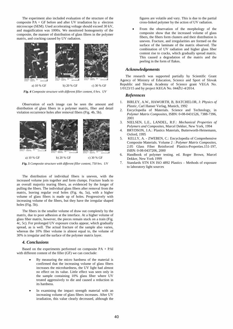
The experiment also included evaluation of the structure of the composite PA + GF before and after UV irradiation by a electron microscope (SEM). Used accelerating voltage should exceed 30 kV, and magnification was 1000x. We monitored homogeneity of the composite, the manner of distribution of glass fibres in the polymer matrix, and cracking caused by UV radiation.
a) 10 % GF b) 20 % GF c) 30 % GF
Fig. 4 Composite structure with different filler content, 0 hrs. UV
Observation of each image can be seen the amount and distribution of glass fibers in a polymer matrix, fiber and detail violation occurrence holes after removal fibers (Fig. 4b, 5b).
a) 10 % GF b) 20 % GF c) 30 % GF
Fig. 5 Composite structure with different filler content, 750 hrs. UV
The distribution of individual fibers is uneven, with the increased volume join together and form clumps. Fracture leads to an overall majority tearing fibers, as evidenced by the longer of pulling the fibers. The individual glass fibers after removal from the matrix, leaving regular oval holes (Fig. 4a, 5a), with a higher volume of glass fibers is made up of holes. Progressively with increasing volume of the fibers, but they have the irregular shaped holes (Fig. 5b).
The fibers in the smaller volume of draw out completely by the matrix, due to poor adhesion at the interface. At a higher volume of glass fiber matrix, however, the pieces remain stuck on a train (Fig. 4c, 5c). For prolonged UV exposure cracks appear, which gradually spread, as is well. The actual fracture of the sample also varies, whereas the 10% fiber volume is almost equal to, the volume of 30% is irregular and the surface of the polymer matrix layer.
4. Conclusions Based on the experiments performed on composite PA + PAI
with different content of the filler (GF) we can conclude:
• By measuring the micro hardness of the material is confirmed that the increasing volume of glass fibers increases the microhardness, the UV light had almost no effect on its value. Little effect was seen only in the sample containing 10% glass fiber where UV treated aggressively to die and caused a reduction in its hardness.
• In examining the impact strength material with an increasing volume of glass fibers increases. After UV irradiation, this value clearly decreased, although the
figures are volatile and vary. This is due to the partial cross-linked polymer by the action of UV radiation.
• From the observation of the morphology of the composite show that the increased volume of glass fibers, the fibers form clusters and their distribution is uneven. Fracture, and irregularities are formed on the surface of the laminate of the matrix observed. The combination of UV radiation and higher glass fiber content rise to cracks, which gradually spread matrix. This caused a degradation of the matrix and the peeling in the form of flakes.
Acknowledgements The research was supported partially by Scientific Grant
Agency of Ministry of Education, Science and Sport of Slovak Republic and Slovak Academy of Science grant VEGA No. 1/0123/15 and by project KEGA No. 044ŽU-4/2014.
References 1. BIRLEY, A.W., HAWORTH, B, BATCHELOR, J: Physics of
Plastic, Carl Hanser Verlag, Munich, 1992 2. Encyclopedia of Materials. Science and Technology, in
Polymer Matrix Composites, ISBN: 0-08-0431526, 7388-7396, 2001
3. NIELSEN, L.E., LANDEL, R:F.: Mechanical Properties of Polymers and Composites, Marcel Dekker, New York, 1994
4. BRYDSON, J.A.: Plastics Materials, Butterworth-Heinemann, Oxford, 1995
5. KELLY, A. - ZWEBEN, C.: Encyclopedia of Comprehensive Composite Materials. Volume 2 : Polymer Matrix Composites, 2.05 Glass Fiber Reinforced Plastics-Properties.151-197, ISBN: 0-08-0437206, 2000
6. Handbook of polymer testing. ed. Roger Brown, Marcel Dekker, New York 1999
7. Standards STN EN ISO 4892 Plastics – Methods of exposure to laboratory light sources
40

POLYESTER/SILICATE COMPOSITES
ПОЛИЕСТЕРНО-СИЛИКАТНИ КОМПОЗИТИ
Assoc. Prof. Cherkezova R. PhD.1, Assoc. Prof. Radenkov Ph. PhD.2, Asst. Prof. Zafirova K.1, Assoc. Prof. Popov A. PhD.3, Asst. Prof.
Hristova Т. PhD.1, Assoc. Prof. Radenkov M. PhD.2, Senior Asst. Prof. Todorov N. PhD.3 Medical University „Prof. Dr. Paraskev Stoyanov“- Varna1, Technical University - Sofia2, University „Prof. Dr. Asen Zlatarow “ – Burgas3,
Bulgaria E-mail: [email protected], [email protected], [email protected], Tatiana. [email protected],
[email protected], [email protected] Abstract This work is a continuation of the HUPER development, as in this study hydrophilization was performed by different types of cement (grey cement and medical cement). It was established that alkaline hydroxides in the cement “milk” composition traditionally perform the preselected role of a hydrophilizer. Water was used as a second dispersing component, which can not only homogenize the composition of the prepared composite material. A third component was introduced (water glass), which was studied due to its dispersing role towards the resin/cement/water system. Mechanical strength characteristics (mostly impact characteristics) characterizing the shape, dimensions and integrity of the operational product were studied based on the obtained composition in various proportions of components. KEYWORDS: hydrophilization, resin/mineral disperse system, cement, water glass. 1. Introduction The development of composites based on hydrophilized unsaturated polyester resin (HUPER) could be accomplished not only by methods described in previous works [1-5] but also with different types of cement (Sulfate-resistant blastfurnace cement and medical cement). The addition of cement affects the curing behavior compared to the unmodified resin, which is important for tracing the polymerization. The investigation of mechanical indices of the compositions obtained is another essential task in terms of their main purpose as polymer/silicate composites. Some literary sources review the role of cement as a supplement demonstrating the various advantages of modified resins: for obtaining artificial stone [6]; possibilities for producing repair materials [7]; for strength and elasticity modulus optimization [8]. Cement-based composites were also obtained as cement was used as a filler in a fiberglass/polyester resin matrix in view of sea-water resistance [9]. The purpose of this work is the development of UPER-based compositions in view of their application as composite materials – polymer concrete, fiberglass, etc. 2. Materials and methods 2.1. Materials We used: Resin of type Vinalkyd 550 PE-R (Orgachim Resins – Ruse) containing 35% styrene and 65% unsaturated polyesters, which is a condensation product of propylene glycol and maleic anhydride. A 50% solution of cyclohexanone perodxide (CHP) in dibutylphthalate was used as a curing initiator, and a 10% solution of cobalt naphthenate (CN) in styrene was the accelerator. Medical two-compound zinc phosphate cement in the form of powder, ADHESOR® - „SpofaDental“ (MC). Sulfate-resistant blastfurnace cement CEM III A-S 42.5 N SR – Devnya Cement, town of Devnya (SC). Sodium silicate solution (Water glass - WG) – BEKO Water Glass and Detegrents Factory, town of Troyan
2.2. Methods Methods for obtaining compositions based on unsaturated polyester resin (UPER) hydrophilized with different types of cement (SC and MC) have been developed at fixed amount of water compared to cement (50%) in the presence or absence of WG, at fixed CN/CHP ratio compared to resin. Charpy impact strength tests have been performed to test pieces using Ceast 6545/000, Great Britain. A test piece fixed next to its ends as a horizontal beam is hit by a single pendulum impact. The impact direction is in-between the supports holding the test piece at fixed speed of 50 mm/min. The impact energy absorbed by the test piece is reported. Test pieces were tested for pressure strength by dynamometer Instron 4203, Great Britain. The test piece is pressure loaded at a fixed rate of strain of 50 mm/min, until destroyed. 3. Results and discussion Polymeric compositions have been developed with various quantities of SC at a constant cement to water ratio (2:1), the same amount of UPER curing in the presence of CN/CHP redox system (table 1). A composition without SC was produced for comparison. The polymerization of UPER was traced in the presence of different percentage of SC compared to resin. It was found that with increase in its amount, within the range from 10% to 40%, the maximum temperature gradually decreased from 140 to 60 ˚C (fourfold decrease). The kinetics of the polymerization process of UPER in the absence of SC shows that the unmodified resin has the highest curing temperature and the least gelation time (fig.1).
41

Table 1. Data on the obtaining of composites based on UPER hydrophilized with different quantities of SC. Quantities: UPER – 30 g, CN – 0.5 ml, water – 50% vs. SC quantity, CHP – 1 ml
Composition No.
SC quantity %
Time [τ, min]
Temperature T max., ˚C]
1 - 9 154
2 12.82 14 139.5
3 21.50 22 124.5
4 27.78 27 101
5 32.52 30 84.5
6 36.23 35 70.5
7 39.21 37 61.5
Fig. 1. Kinetics of the polymerization process, where curve 1 – 0% SC, curve 2 – 12.82% SC, curve 3 – 21.5% SC, curve 4 –
27.78% SC, curve 5 – 32.52% SC, curve 6 – 36.23% SC, curve 7 – 39.21% SC (according to Table 1) The impact and pressure strengths of the compositions in table 1 have been studied as shown in fig. 2 and fig. 3, respectively. Fig. 2 shows that the increased percent content of SC results in increase of the impact strength compared to the zero sample, as such dependency is of extremal nature – at about 22 ±2% and 35±2% SC reaches maximums and at 27±2% and 35± % SC reaches minimums.
Fig. 3 shows the change in the pressure strength according to the SC quantity, where the most significant increase is at 15% SC. Further increase in the cement quantity does not lead to significant increase in that inedx, while the high value trend is preserved.
Fig. 3. Data on the pressure strength when changing the SC quantity
(according to Table 1). The influence of a third component (WG) was studied and for that purpose, compositions at fixed amount of SC (21,5%) were developed. The respective composition in the absence of WG was produced for comparison (No. 1, table 2). Table 2. Data on the obtaining of composites based on UPER hydrophilized with the same quantity of SC when changing the amount of WG. Quantities: UPER – 30 g, CN – 0.5 ml, SC – 21,5%, water – 50% vs. SC quantity, CHP – 1 ml
Composition No.
WG quantity %
Time [τ, min]
Temperature [T max., ˚C]
1 - 22 124.5
2 2.52 42 97.5
3 4.91 41 90.5
4 7.18 35 99.5
5 9.36 39 83.5
6 11.43 39 75.5
The kinetics of polymerization processes was traced according to the WG content and the strength indices of such compositions and certain main conclusions were made concerning the obtained result. Those conlcusions will be presented in our following works. Polymeric compositions have beem also developed with different quantities of MC (MC:water=2:1), at a fixed amount of UPER and redox system (table 3).
Fig. 2. Data on the impact strength when changing the SC quantity (according to Table 1).
42
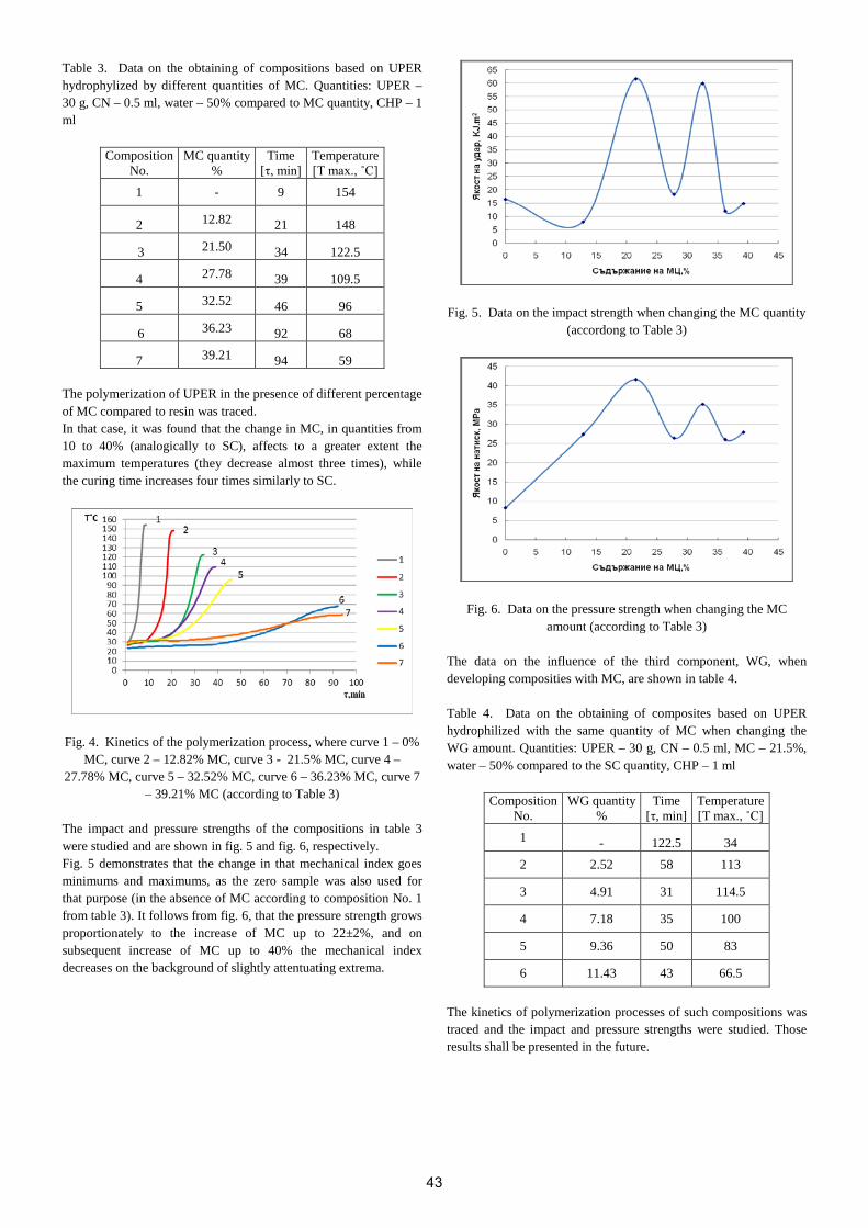
Table 3. Data on the obtaining of compositions based on UPER hydrophylized by different quantities of MC. Quantities: UPER – 30 g, CN – 0.5 ml, water – 50% compared to MC quantity, CHP – 1 ml
Composition No.
MC quantity %
Time [τ, min]
Temperature [T max., ˚C]
1 - 9 154
2 12.82 21 148
3 21.50 34 122.5
4 27.78 39 109.5
5 32.52 46 96
6 36.23 92 68
7 39.21 94 59 The polymerization of UPER in the presence of different percentage of MC compared to resin was traced. In that case, it was found that the change in MC, in quantities from 10 to 40% (analogically to SC), affects to a greater extent the maximum temperatures (they decrease almost three times), while the curing time increases four times similarly to SC.
Fig. 4. Kinetics of the polymerization process, where curve 1 – 0% MC, curve 2 – 12.82% MC, curve 3 - 21.5% MC, curve 4 –
27.78% MC, curve 5 – 32.52% MC, curve 6 – 36.23% MC, curve 7 – 39.21% MC (according to Table 3)
The impact and pressure strengths of the compositions in table 3 were studied and are shown in fig. 5 and fig. 6, respectively. Fig. 5 demonstrates that the change in that mechanical index goes minimums and maximums, as the zero sample was also used for that purpose (in the absence of MC according to composition No. 1 from table 3). It follows from fig. 6, that the pressure strength grows proportionately to the increase of MC up to 22±2%, and on subsequent increase of MC up to 40% the mechanical index decreases on the background of slightly attentuating extrema.
Fig. 5. Data on the impact strength when changing the MC quantity (accordong to Table 3)
Fig. 6. Data on the pressure strength when changing the MC amount (according to Table 3)
The data on the influence of the third component, WG, when developing composities with MC, are shown in table 4. Table 4. Data on the obtaining of composites based on UPER hydrophilized with the same quantity of MC when changing the WG amount. Quantities: UPER – 30 g, CN – 0.5 ml, MC – 21.5%, water – 50% compared to the SC quantity, CHP – 1 ml
Composition No.
WG quantity %
Time [τ, min]
Temperature [T max., ˚C]
1 - 122.5 34 2 2.52 58 113
3 4.91 31 114.5
4 7.18 35 100
5 9.36 50 83
6 11.43 43 66.5 The kinetics of polymerization processes of such compositions was traced and the impact and pressure strengths were studied. Those results shall be presented in the future.
43

4. Conclusion There are alternating maximums and minimums and it is determined by different factors, polyemrization first; moreover, there may be emulsion of cement milk in the resin, as at higher concentrations, there will be emulsion of resin in the cement milk, respectively. Therefore, phase inversion could be expected at higher concentrations. It can be assumed that the emulsion containing drop-shaped cement milk cures before the resin and vice versa, where cement cures slowly, resin cures first. It could be expected that interpenetrating polymer/silicate networks have been obtained. In such cases, curves necessarily follow minimums and maximums and when the curves are of the right Gaussian character, it would mean that polymer-silicate mechanical blends were obtained. At the same time, although the polymer and silicate are two different skeletons, they are interconnected because each resion molecule has turned into soap. And the soap moistens and interacts with cement, which does not inhibit the resin polymerization. Indeed, we have a lot of mazimums and minimums and very complex processes are under way, apparently depending on the polymerization process activity, sample compositions and structure formation processes. The completion of the polymerication process puts an end to resin curing and cement curing. 5. References
1. Radenkov, M., V. Trenev, V. Dikov, R. Cherkezova, Ph. Radenkov. On the noxious influence of the excess of moisture during polymer concrete obtaining. Mechanics and Technology of Composite Materials. 2009, 238-42.
2. Radenkov, M., V. Trenev, V. Dikov, R. Cherkezova, Ph. Radenkov. An Approach to Eliminate the Adverse effect of Increased Humidity on Formation of Polymer Concrete. Mechanics and Technology of Composite Materials. 2009, 242-48.
3. Черкезова, Р; 2001. Многокомпонентна полимерна система на основата на хидрофилизирана ненаситена полиестерна смола и методи за получаването й. BG Patent 63168.
4. Cherkezova, R; An. Topliyska, F. Radenkov, B. Milosheva. Dynamics of hardening of polyester-silicate adaptive compositions for binding silicate concrete with polyester polymer concrete. Journal of polymer engineering. 2005, 1(25), 11-21.
5. Cherkezova, R., Ph. Radenkov, M. Radenkov, T. Hristova, K. Zafirova, N. Todorov, A. Popov. Hydrophilization of unsaturated polyester resin with sulfur, sodium hydroxide and water with a possibility for its curing in the presence of water as a solvent. In: Materials, Methods & Technologies, 26-30 June 2016. J. Int. Sci. Pub., 10, 2016.
6. Sarami, N., L. Mahdavian. Comparison of artificial stone made from sludge stone with travertine stone waste of stone cutting factory. Int. J. Eng. Res. Africa, 23, 2016, 64-71.
7. Adi Kristiawan, S., A. Bekti Prakoso. Flexural behaviour of patch-repair material made from unsaturated polyester resin (UPR)-mortar.In: International Conference on Advanced Materials Engineering and Technology, ICAMET 2015; Kaohsiung; Taiwan; 4 - 5 December 2015. Materials Science Forum, 857, 2016, 426-30.
8. Gupta, S.U.C., V.N. Pillai, S.S. Gupta. Development of hovercraft landing base/platform at seashore by cementicious MF polymer sea-sand composites. Recent Innovations in Chem. Eng, 8(1), 2015, 43-56.
9. Shettar, M., P. Hiremath. Effect of seawater on mechanical properties of GFRP with cement as filler material for fishing boat application. Int. J. Appl. Eng. Res., 10(19), 2015, 40027-30.
44

EFFECT OF PLASTIC DEFORMATION ON THE MICROSTRUCTURE AND PLASTICITY OF HIGH FREQUENCY ELECTRIC RESISTANCE WELDING
Prof. Dr. Maksuti Rr.
Faculty of Applied Sciences, State University of Tetova, Republic of Macedonia
Abstract: High frequency electric resistance welding is one of the most extensively used methods for production of longitudinally welded carbon steel pipes suitable for line pipe, casing and tubing. In this pipe production process, the hot rolled steel strip goes into the continuous cold forming process and its edges are continuously joined by a combination of localized high-frequency electric resistance heating and plastic deformation. The heated edges up to the welding temperature squeezed together at the “Vee” apex by the forge pressure rolls, plastically deformed and a forge type weld is formed. The plastic deformation which is realized under the action of the squeezing rolls caused changes of the microstructure constituents in the bond line and in the heat affected zone and plays principal role on the quality of the welded joint. In this paper microstructure and plasticity of the welded joint were investigated by light microscopy and flattening testing. The obtained results shows that plastic deformation plays principal role on the microstructure and plasticity of the welded joint.
KEYWORDS: MICROSTRUCTURE, PLASTIC DEFORMATION, HIGH FREQUENCY WELDING, PLASTICITY.
1. Introduction High-frequency electric resistance welding (HFERW) process
is one of the most extensively methods for production of high quality longitudinal seam welded carbon steel pipes suitable for line pipe, casing and tubing. In this process, hot rolled strip is gradually formed into round shape through roll-forming stands, and its edges are joined by a combination of localized high-frequency electric resistance heating and forge pressure, as schematically illustrated in Figure 1 [1,2,3]. Most of these pipes are produced according to API Standard [4] plus client supplementary requirements. Under this heat input condition and forge pressure it is possible to improve the weld joint quality and productivity of longitudinal seam welded carbon steel pipes.
Fig.1 Schematic illustration of HFERW
The high-frequency current applied to the strip edges through sliding contacts, concentrated on the surface layer of the strip edges due to the “skin” and “proximity” effects, generate joule heat and the hot “ Vee” converge edges are forged together in the weld squeeze rolls and a forge type weld is achieved [5]. The HF weld is a true forge weld in that no filler metal is added and, if done properly, no molten or oxidized metal is left on the bond line.
One of the most important factor in the high frequency electric resistance welding (HFERW) is plastic deformation which is present in the entire manufacturing process, from the beginning to the end of the manufacturing process. Almost in all manufacturing operations, plastic deformation directly or indirectly participates on the development of these operations at room temperatures or at elevated temperatures. Depending on the intensity of cold plastic deformation and the sizes of pipes (diameter and wall thickness), it can happen changes of mechanical properties, i.e. strength increased due to work hardening or decreased due to Bauschinger effect [6].
Figure 2 shows that during HFERW, all of the molten thin layer and metal oxides and other inclusions are squeezed out of the weld toward the outside and inside surfaces as a result of plastic deformation of the squeezing rolls.
Fig.2 Effect of plastic deformation on the HFERW
The material extruded on the inside and outside weld surfaces, usually removed by scarfing while still hot and forms a typical HFERW weld with narrow bond line (BL) or fusion line (FL) and associated local heat affected zone (HAZ) is formed [5]. The high frequency electric resistance welded seam is subjected to post weld heat treatment in-line such as induction heating and gradually air cooling, the purpose of which is to eliminate zones of excessive hardness from the initial welding process as such zones could be susceptible to various forms of environmental cracking.
The plastic deformation which is realized under the action pressure of the squeezing rolls caused metal flows of the hot rolled coils towards the outside and inside surfaces of the bond line. This flow pattern consists of streaks and striations. The orientation of this pattern, with respect to the new surface, indicates the direction of metal flow lines (fibres), respectively flow angles during plastic deformation [6]. The flow lines, respectively flow angles (α1, α2, α3, α4), Figure 3, are a natural consequence of applied plastic deformation of the squeezing rolls. The orientation of the flow lines indicates the direction of the metal flow during plastic deformation. By the measurement of the flow angles (α1, α2, α3, α4) and especially flow angle (α1+α3), it is possible to determine directly whether the squeezing pressure and relevant welding temperature are correct or not.
Fig.3 Flow lines (fibres) and flow angles around bond line during
plastic deformation
45

Microstructural changes that takes place during the HFERW covers the properties of the welded pipes, defects associated with welding and the performance of welded pipes in service.
Forge weld area of HFERW may be divided into four zones, Figure 4, [7]: 1-bond line (BL) or fusion line (FL); 2-heat affected zone (HAZ); 3-edge of the heat affected zone and 4-base metal or parent metal (BM). These different zones are normally defined by the peak temperature experienced at certain distance from the fusion line during welding. Each zone in the weld area is characterized by a unique microstructure and hence different mechanical properties. The zones of the weld area are quite narrow and it is difficult to investigate the behavior of specific location without interference from the adjacent zones with different properties.
Fig.4 Schematic illustration of constitutive parts of weld area
2. Experimental procedure High-frequency electric resistance welding was conducted using
an L-16 in, pipe mill Newco IMK-Ferizaj, Kosova. Newco IMK-Ferizaj-Kosova produces high frequency electric resistance longitudinal seam welded steel pipes with Ø114.3-406.4mm diameter and 3.2-12.7mm wall thickness. Casing pipes Ø114.3x5.21mm are typical case in the mill production schedule, hence in this paper these pipes were investigated. Pipes Ø114.3x5.21mm were fabricated from high strength steel coils J55 according to API [4] standard, using the pipe mill equipped with a contact type high frequency electric resistance welding machine-Thermatool. The frequency of current was 400kHz.
Chemical composition and mechanical properties of the used steel are given in Table 1 and 2.
Table 1: Chemical composition of used steel coils J55
Steel coils
Chemical composition [wt-%]
C Mn Si P S Al Nb N
API grade J55
0.141 1.113
0.229
0.014
0.008
0.047
0.017 0.0072
Table 2: Mechanical properties of used steel coils J55
Steel coils
Mechanical properties
Re Rm A2”
[MPa] [%]
API grade J55
453 557 32.5
The influence of plastic deformation can be observed by examining the flow lines, respectively flow angles around fusion (bond) line.
The flow lines are visible in all metallographic specimens and the degree of upset is different, depending from the intensity of plastic deformation of squeeze weld rolls.
Under the action of plastic deformation, the squeezing amount (Sa), Figure 5 is defined as the difference between the circumference length measured at “Vee” angle in the front of the squeezing rolls and at pipes in the rear of squeezing rolls, which is usually 1-5mm. In this paper squeezing amount (Sa=Cb-Ca) varies from 1.7-5.9mm.
Fig.5 Squeezing amount during HFERW
Plasticity of welded joint was confirmed by conducting flattening testing [4].
In order to determine metallographic macro and micro analysis, the metallographic specimens were prepared by standard metallographic techniques that includes grinding, polishing and etching with suitable etchant (nital and Oberhoffer) to reveal the macro and microstructure.
For the experimental procedure, pipe rings (10-15cm long) were extracted from several pipes for use as the specimens, Figure 6.
Fig.6 Sketch illustrating the used specimens
3. Results and discussion Figure 7 shows the effect of plastic deformation on the flow
lines and flow angles depending on the squeezing amount (Sa=1.7-5.9mm).
The flow lines and flow angles (α1,α2,α3, α4, α1+α3 and α2+α4) were measured separately for each cases of squeezing amount and obtained results were presented in the relevant illustration in Figure 7, together with the values of the squeezing amount at the bottom of the right side of the illustrations. From the presented illustrations in Figure 7 it is clear that increasing of plastic deformation, respectively increasing of the squeezing amount, increased the orientation of flow lines towards the outside and inside of wall thickness. Flow angles also increased with the increasing of plastic deformation and should be noted that for small angles (α1+α3<50o), “Y” flow, Figure 8a, in the outside weld joint were occurred cracks. Cracks or breaks were occurred also for larger angles (α1+α3>70o), “T” flow, figure 8b. Optimal values for (α1+α3) were 60±10o. Plasticity of the welded joint, in this case
46

measured by the flattening testing is good only for optimal values of (α1+α3=60±10 o).
Fig.7 Flow lines and flow angles depending on the squeezing
amount
(a) (b)
Fig.8 Metal flow during HFERW :a-“Y” flow, b-“T” flow
The test specimens for flattening testing were flattened in a hydraulic press, DIHNAFORIN PS 2043, at room temperature between to parallel plates with the weld line located 90o and 0o to the applied force. The specimens (rings) were flattened to a specified height (h=2/3D=76.2mm) according to API, Figure 9.
Fig.9 Schematic illustration of flattening test
During flattening testing, in some rings were occurred cracks or breaks in the weld area in the position (90o and 0o) before specified height (h=76.2mm) according to API. Figure 10 shows the results of the flattening testing of all tested specimens.
Correlation between squeezing amount (Sa) and flow angle (α1+α3), Figure 11 (red rectangle) shows that optimal values of squeezing amount (Sa) are in the range 2.5-3.5mm for manufacturing of HFERW pipes Ø114.3x5.21mm from high strength steel coils J55 according to API in line L-16, at the pipe mill Newco IMK-Ferizaj, Kosova.
Fig.10 Plasticity of the welded joint
Fig.11 Correlation between Squeezing amount (Sa) and flow
angle (α1+α3)
47
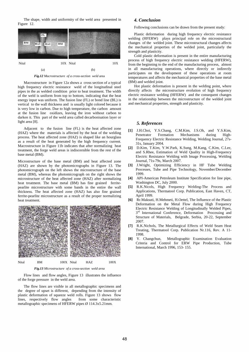
The shape, width and uniformity of the weld area presented in Figure 12.
Nital 10X Nital 10X
(a) (b)
Fig.12 Macrostructure of a cross-section weld area
Macrostructure in Figure 12a shows a cross section of a typical high frequency electric resistance weld of the longitudinal steel pipes in the as welded condition prior to heat treatment. The width of the weld is uniform from top to bottom, indicating that the heat energy input was uniform. The fusion line (FL) or bond line (BL) is vertical to the wall thickness and is usually light colored because it is very low in carbon. Due to high temperature, the carbon amount at the fusion line oxidizes, leaving the iron without carbon to darken it. This part of the weld area called decarbonisation layer or light area [8].
Adjacent to the fusion line (FL) is the heat affected zone (HAZ) where the materials is affected by the heat of the welding process. The heat affected zone (HAZ) is shaped like an hourglass as a result of the heat generated by the high frequency current. Macrostructure in Figure 11b indicates that after normalizing heat treatment, the forge weld areas is indiscernible from the rest of the base metal (BM).
Microstructure of the base metal (BM) and heat affected zone (HAZ) are shown by the photomicrographs in Figure 13. The photomicrograph on the left shows the microstructure of the base metal (BM), whereas the photomicrograph on the right shows the microstructure of the heat affected zone (HAZ) after normalizing heat treatment. The base metal (BM) has fine grained ferrite-pearlite microstructure with some bands in the entire the wall thickness. The heat affected zone (HAZ) has also fine grained ferrite-pearlite microstructure as a result of the proper normalizing heat treatment.
Nital BM 100X Nital HAZ 100X
Fig.13 Microstructure of a cross-section weld area
Flow lines and flow angles, Figure 13 illustrates the influence of the forge pressure in the weld area.
The flow lines are visible in all metallographic specimens and the degree of upset is different, depending from the intensity of plastic deformation of squeeze weld rolls. Figure 13 shows flow lines, respectively flow angles from some characteristic metallographic specimens of HFERW pipes Ø 114.3x5.21mm.
4. Conclusion Following conclusions can be drawn from the present study: Plastic deformation during high frequency electric resistance
welding (HFERW) plays principal role on the microstructural changes of the welded joint. These microstructural changes affects the mechanical properties of the welded joint, particularly the strength and plasticity.
Cold plastic deformation is present in the entire manufacturing process of high frequency electric resistance welding (HFERW), from the beginning to the end of the manufacturing process, almost in all manufacturing operations, where directly or indirectly participates on the development of these operations at room temperatures and affects the mechanical properties of the base metal (BM) and welded joint.
Hot plastic deformation is present in the welding point, where directly affects the microstructure evolution of high frequency electric resistance welding (HFERW) and the consequent changes in the relationship between the microstructure of the welded joint and mechanical properties, strength and plasticity.
5. References [1] J.H.Choi, Y.S.Chang, C.M.Kim, J.S.Oh, and Y.S.Kim,
Penetrator Formation Mechanisms during High- Frequency Electric Resistance Welding, Welding Journal, 27s-31s, January 2004.
[2] D.Kim, T.Kim, Y.W.Park, K.Sung, M.Kang, C.Kim, C.Lee, and S.Rhee, Estimation of Weld Quality in High-Frequency Electric Resistance Welding with Image Processing, Welding Journal, 71s-79s, March 2007.
[3] J.Wright, Optimizing Efficiency in HF Tube Welding Processes, Tube and Pipe Technology, November/December 1999.
[4] API-American Petroleum Institute Specification for line pipe, Washington DC, July 2000.
[5] R.K.Nicols, High Frequency Welding-The Process and Applications, Thermatool Corp. Publication, East Haven, CT, April 1999.
[6] Rr.Maksuti, H.Mehmeti, H.Oettel, The Influence of the Plastic Deformation on the Metal Flow during High Frequency Electric Resistance Welding of Longitudinally Welded Pipes, 3rd International Conference, Deformation Processing and Structure of Materials, Belgrade, Serbia, 20-22, September 2007.
[7] R.K.Nichols, The Metallurgical Effects of Weld Seam Heat Treating, Thermatool Corp. Publication Nr.116, Rev. A 11-1998.
[8] Y. Changchun, Metallographic Examination Evaluation Criteria and Control for ERW Pipe Production, Tube International, March 1996, 153- 155.
48