technical report effects of mergers involving...
TRANSCRIPT

Technical Report Effects of Mergers Involving Differentiated Products
COMP/B1/2003/07
Roy J. Epstein*
Daniel L. Rubinfeld†
October 7, 2004
INTRODUCTION AND SUMMARY
This Technical Report is offered in accordance with our contract to develop
protocols and software for horizontal merger review under COMP/B1/2003/07. The
report is divided into five sections. Section I is an overview of merger simulation
methods, including estimation of the necessary elasticities to calibrate a simulation
model. We discuss econometric estimation of a full AIDS demand system as well as use
of logit and PCAIDS models that incorporate restrictions that allow one to perform
simulation with much less data. Adding �nests� allows specification of more general
logit and PCAIDS models with fewer restrictions on elasticities. In this Report we
discuss nests within the PCAIDS framework and show how they may be parameterized
exogenously or calibrated based on observed profit margins. We also compare the
properties of AIDS, logit, and PCAIDS, since each of these models is likely to predict
somewhat different price effects from mergers.
Section II discusses �Critical Loss Analysis� (�CLA�), which has become a widely
used methodology for analyzing market definition and competitive effects. We describe
the CLA calculation and we review recent literature that discusses interpretation and
potential misuse of CLA. We also describe how CLA relates to merger simulation, since
the two approaches share important similarities. For example, a recent reformulation of
CLA in terms of �diversion ratios� is very similar to the use of cross-price elasticities to
* Adjunct Professor of Finance, Boston College, Chestnut Hill, MA USA. Email: [email protected]. † Robert L. Bridges Professor of Law and Professor of Economics, University of California, Berkeley.
Email: [email protected].

ii
calibrate a merger simulation model. This section also describes how CLA and merger
simulation can be applied to study coordinated effects.
Section III discusses geographic market definition. We review the leading articles
on methodology and discuss the practical issues of implementing such methodologies.
Experience has shown that the geographic market definition often has to be developed
using facts that are highly specific to the case at hand, since suitable datasets for
econometric estimation are often not available in a merger investigation. We discuss the
role of limited �natural experiments� in interpreting the data on market definition and we
compare the analysis used by the parties in Volvo Scania.
Section IV describes the econometric software for demand system estimation and
unilateral effects simulation. Section V presents two case studies of estimation and
simulation. It also includes commentary on geographic market definition and other
aspects of unilateral effects analysis raised in the litigated U.S. v. Oracle merger case.
There are two appendices. Section VI is a detailed technical appendix that
summarizes the analytical details associated with the econometric estimation of demand
models using scanner data and with the simulation of the likely price effects of mergers.
Section VII reproduces the full text of the 2002 Antitrust Law Journal article by Epstein
and Rubinfeld that introduced PCAIDS. The article is included as a convenience for the
reader since there are frequent references to it in this Report.

iii
CONTENTS I. OVERVIEW OF MERGER SIMULATION................................................................................ 1
A. INTRODUCTION............................................................................................................................ 1 B. PARAMETER REDUCTION IN DEMAND MODELS............................................................................. 3
1. Independence of Irrelevant Alternatives (�IIA�) ..................................................................... 3 2. Multi-Stage Budgeting Models and AIDS................................................................................ 5
C. ALM STRUCTURE ....................................................................................................................... 6 D. AIDS STRUCTURE AND ESTIMATION............................................................................................ 9 E. PCAIDS ................................................................................................................................... 11
1. PCAIDS Calibration without Nests ....................................................................................... 12 2. Deviations from Proportionality � PCAIDS with Nests ........................................................ 12 3. Using Brand-Level Profit Margins to Calibrate PCAIDS with Nests...................................... 14
F. GENERAL SOLUTION OF THE POST-MERGER FOCS...................................................................... 17 G. SIMULATION AND PRODUCT MARKET DEFINITION ...................................................................... 19 H. THE CHOICE OF MERGER SIMULATION MODEL ........................................................................... 21
1. The Bertrand Assumption ..................................................................................................... 21 2. Testing IIA ........................................................................................................................... 22 3. Comparing the ALM, PCAIDS, and AIDS ............................................................................. 24
I. MERGER SIMULATION BIBLIOGRAPHY........................................................................................ 25 1. Foundational Analyses of Demand and Industrial Organization............................................ 25 2. Specification and Use of ALM, AIDS, and PCAIDS Models................................................... 25 3. Additional Merger Simulation Demand Models..................................................................... 27
II. CRITICAL LOSS ANALYSIS.................................................................................................... 28 A. INTRODUCTION.......................................................................................................................... 28 B. CLA AND DIVERSION RATIOS .................................................................................................... 30 C. COORDINATION ......................................................................................................................... 32 D. CRITICAL LOSS BIBLIOGRAPHY .................................................................................................. 33
III. GEOGRAPHIC MARKET DEFINITION............................................................................. 34 A. OVERVIEW ................................................................................................................................ 34 B. APPROACHES TO GEOGRAPHIC MARKET DEFINITION .................................................................. 35
1. Elzinga-Hogarty Tests .......................................................................................................... 35 2. Price Correlations................................................................................................................ 37 3. Granger Causality and Cointegration................................................................................... 38 4. Other Methodologies............................................................................................................ 41
C. GEOGRAPHIC MARKET DEFINITION BIBLIOGRAPHY .................................................................... 43 IV. ECONOMETRIC SOFTWARE............................................................................................. 45
A. STATA PROGRAMS FOR ECONOMETRIC DEMAND SYSTEM ESTIMATION........................................ 45 B. ESTIMATION AND ENDOGENEITY................................................................................................ 47 C. DG-COMP MSP EXCEL MENU COMMANDS .............................................................................. 48 D. IMPORTING STATA ESTIMATION RESULTS INTO DG-COMP MSP................................................ 56
1. AIDS.................................................................................................................................... 56 2. Logit .................................................................................................................................... 58
V. CASE STUDIES .......................................................................................................................... 61 A. BEER......................................................................................................................................... 61
1. AIDS Beer Estimation Results............................................................................................... 62 2. Logit Beer Estimation Results............................................................................................... 62 3. Beer Simulation Results........................................................................................................ 62
B. TOILET TISSUE .......................................................................................................................... 63 1. AIDS Tissue Estimation Results ............................................................................................ 64

iv
2. Logit Tissue Estimation Results ............................................................................................ 64 3. Tissue Simulation Results ..................................................................................................... 65
C. BUSINESS SOFTWARE ................................................................................................................ 66 1. Geographic Market .............................................................................................................. 67 2. Unilateral Effects ................................................................................................................. 68
VI. TECHNICAL APPENDIX ..................................................................................................... 71 A. NOTATION................................................................................................................................. 71 B. ECONOMETRIC ESTIMATION....................................................................................................... 72
1. ALM..................................................................................................................................... 72 2. AIDS.................................................................................................................................... 73
C. SHARES AND ELASTICITIES FOR THE SIMULATION MODELS ......................................................... 74 1. ALM..................................................................................................................................... 74 2. AIDS.................................................................................................................................... 75 3. PCAIDS ............................................................................................................................... 75
D. FIRST-ORDER CONDITIONS FOR SIMULATION.............................................................................. 78 1. Pre-Merger .......................................................................................................................... 78 2. Post-Merger......................................................................................................................... 79
E. SOLUTION EXAMPLES ................................................................................................................ 80 1. ALM..................................................................................................................................... 80 2. AIDS.................................................................................................................................... 82 3. PCAIDS ............................................................................................................................... 83 4. PCAIDS with Nests............................................................................................................... 85
VII. APPENDIX: MERGER SIMULATION: A SIMPLIFIED APPROACH WITH NEW APPLICATIONS.................................................................................................................................. 87

1
I. OVERVIEW OF MERGER SIMULATION
A. Introduction
Merger simulation is a set of quantitative techniques to predict price effects of
mergers with differentiated goods. Applied to unilateral effects analysis, it has been used
to assess the magnitude of merger-specific efficiencies (reductions in marginal costs for
the merging firms) required to offset predicted price increases and to evaluate the
adequacy of proposed divestitures. Simulation can also help analyze the competitive
effects of product repositioning and de novo entry. The development of simulation
methods is continuing and the scope of their possible application is being broadened. For
example, we will describe potential applications of simulation methods to the evaluation
of coordinated effects and to Critical Loss Analysis.
In the history of merger analysis, merger simulation is a relatively new entrant. It
has been used by the U.S. competition authorities since the early 1990s. While complex
in its details, merger simulation is appealing because it allows one to generate
quantitative predictions, and (within the framework of a well-specified model) to evaluate
the robustness of those predictions. Put simply, merger simulation takes as a starting
point a model of equilibrium pricing (typically Bertrand), calibrates that model to the
available industry data (such as prices and shares), and uses the model to predict post-
merger price changes.1 Existing techniques focus on the relatively short-term price
effects; a particular transaction may also raise concerns about longer-run issues such as
the rate of product development and innovation that would require separate analysis.
Merger simulation analysis is carried out in two stages. In the first stage, the
estimation of a demand model provides own and cross-price elasticities of demand for the
goods in the pre-merger market. In the second stage, one solves the first-order conditions
(FOCs) for post-transaction profit maximization by the new, post-merger entity. The
post-transaction FOCs differ because they take account of both the cross-price elasticities 1 For recent discussions of the methodology of merger simulation see Epstein and Rubinfeld (2002);
Werden, Froeb, and Scheffman (2004); and Harkrider and Rubinfeld (2004; forthcoming), chapter 11.
2
between the two merging firms and the merger-specific efficiencies. Moreover, the
demand model implies new elasticities as prices change in the new equilibrium. The
solution finds the new post-transaction prices that are consistent with all of these effects.
We discuss three alternative demand models for use in merger simulation. Because
these models have been discussed extensively in the literature, we limit our overview to
their most important features. The models are (i) the antitrust logit model2 (�ALM�); (ii)
the Almost Ideal Demand System3 (�AIDS�), and (iii) the proportionality-calibrated
AIDS known as �PCAIDS.�4 Each model should be viewed as an approximation to the
�true� underlying demand structure. They differ in their data requirements, difficulty in
calibration, flexibility in representing price elasticities, and bottom-line predictions of
price changes.
The ALM requires only market shares, a measure of substitutability between
products, and an estimate of the market demand elasticity. As a tradeoff for the relative
simplicity of its inputs, the ALM relies upon a relatively strong assumption that the cross-
elasticities are identical across products. This assumption will not always be appropriate
in mergers involving differentiated products.
In contrast, AIDS is less restrictive but it requires detailed price and revenue
information, generally supplied by scanner data. AIDS is structurally more complex than
ALM and frequently requires estimation of dozens of coefficients. It can be a significant
econometric challenge to obtain a complete set of coefficients with plausible algebraic
signs, magnitudes, and statistical reliability.
The PCAIDS model offers a simplified version of AIDS that requires only market
shares, an estimate of the market�s demand elasticity, and an estimate of the price
elasticity of demand for a single brand in the market. PCAIDS is similar to the ALM in
assuming in its most basic form that cross-price elasticities between competing products
are equal. PCAIDS and the ALM differ in their underlying mathematical structure,
which leads to different predictions of unilateral effects. When the assumption of equal
2 Werden and Froeb (1994). 3 Hausman, Leonard, and Zona (1994). 4 Epstein and Rubinfeld (2002).
3
cross-price elasticities is not appropriate, both the ALM and PCAIDS can be generalized
by introducing additional �nesting parameters� to make the demand model more flexible.
The models yield different estimates of price effects since elasticities change along
the underlying demand curves as prices increase. Own-price elasticities increase and
cross-price elasticities will also change. Even if all models are matched to the same set
of pre-merger elasticities, the predicted post-merger prices will depend on the �curvature�
of the mathematical relationships that define the demand system.
In this Report we spell out many of the technical details associated with the
application of merger simulation methods. We also discuss factors that might be
considered in deciding whether a particular merger simulation method is appropriate for
the industry being studied. Simulation is an important tool but it should not be used
uncritically or to the exclusion of other possible analyses of mergers involving
differentiated goods.
B. Parameter Reduction in Demand Models
1. Independence of Irrelevant Alternatives (�IIA�)
The demand systems needed to carry out merger simulation are confronted by the
practical problem of estimating a large number of parameters with limited amounts of
data. In general, with N goods there are on the order of N2 unknown own and cross-price
elasticities. Even with scanner datasets, econometric estimation of an unrestricted system
may be infeasible or the results may not be reliable.
The structure of the ALM and PCAIDS incorporates an assumption that greatly
reduces the number of unknown parameters. Specifically, the cross-price elasticities for
all goods with respect to the price of any one other good are the same. Formally, εij = εkj,
where the ε�s are the cross-price and own-price elasticities. Economists refer to this
assumption as the Independence of Irrelevant Alternatives (�IIA�) property.
IIA implies that substitution from any good in the choice set (i.e., market) to all
others in that set is proportional to their relative market shares. Suppose, for example,
that the choice set consists of goods A, B, and C, with respective shares of 60 percent, 30

4
percent, and 10 percent. If the price of good C is increased, the IIA property says that the
substitution to good A must be twice that to B because the share of A is twice that of B.
IIA is a way to define what it means for goods to be equally close substitutes for each
other. If the substitution away from C is proportional to the relative shares of A and B,
then A and B are equally close substitutes for C. The intuition is that if sales of C were
stopped altogether, the sales of A and B would increase by amounts that left their relative
sizes unchanged.
IIA reduces the number of parameters in the system from N2 to 2N, i.e., N own-price
elasticities plus N cross-price elasticities. For markets with 5 brands, for example, it is
only necessary to estimate 10 parameters instead of 25. The ALM, and PCAIDS with
Slutsky-symmetry and homogeneity restrictions from economic theory, in fact have the
property that each system has only two unknown parameters regardless of the number of
brands in the system. This simplification is valuable because it significantly reduces the
data requirements for merger simulation analysis.
IIA provides a convenient basis for inferring substitution patterns if they have not
yet been, or cannot be, estimated. In the absence of reliable evidence to the contrary, a
reasonable assumption is that the merging firms� products are neither especially close nor
especially distant substitutes, which means that IIA applies, at least approximately.5 IIA
also ensures that all estimated elasticities make sense, i.e., that goods assumed to be
substitutes have positive cross elasticities of demand.
If the IIA assumption does not describe the actual market, however, then the
restriction can result in highly inaccurate patterns of substitution. For example, the
implied cross-elasticity can force a high degree of substitution from a luxury car to a
minivan if the minivan has a large share in a �market� defined as all passenger motor
vehicles. Use of IIA is analogous to imposing a set of restrictions on an econometric
model. Restrictions make it possible to obtain values for parameters that either could not
be estimated with the available data, or would be estimated with very low precision.
Imposing valid restrictions allows the remaining parameters to be estimated more
precisely. But imposing invalid restrictions runs the risk of significant bias. 5 See Werden and Froeb (2002) and Willig (1991).

5
When IIA is not appropriate, the alternative is to turn to a more highly parameterized
model of demand. The full AIDS is one possibility, although estimating this model is
data intensive and involves estimating many more parameters. The other possibility is to
specify either the logit or PCAIDS model with nests. In our view, PCAIDS with nests is
often the most appealing alternative because it uses a relatively small number of
additional parameters and is easy to use for sensitivity analyses.
2. Multi-Stage Budgeting Models and AIDS
AIDS is a less restricted system than either ALM or PCAIDS. With no structural
restrictions, there are (N�1)(N+2) parameters. Imposing Slutsky-symmetry and
homogeneity restrictions reduces the number of parameters to (N�1)(N/2+2), which is
still of order N2. Even with relatively large datasets, econometric estimation of so many
coefficients can be problematic, with wrong algebraic signs, implausible magnitudes, and
low statistical reliability for the estimated coefficients.
Restrictions to reduce the number of free parameters in AIDS may be imposed by
assuming a multi-level decision-making process. 6 For example, suppose a dinner entrée
in a restaurant could be beef, lamb, salmon, or trout. An unrestricted AIDS with the four
goods would involve 18 parameters. But suppose customers first choose whether they
want meat or fish, and then make a final choice from the sub-category. This might be
represented as separate meat and fish �markets,� each with two goods. There would be 8
parameters in all, a substantial reduction (in addition, there needs to be additional
structure to determine the initial choice of meat vs. fish).7
Rubinfeld (2000) is a case study of a multi-level model in the context of a merger in
the ready-to-eat (�RTE�) cereal industry. In the RTE industry there are approximately
200 brands. An unrestricted AIDS model would involve nearly 40,000 (200 x 200)
parameters. Simplification is necessary to make the model tractable; such simplification
is usually achieved through a series of relatively strong assumptions about the
6 The concept of multi-level budgeting is due primarily to Gorman (1995). For an exposition, see Maddala
(1988), p. 66. 7 See Hausman, Leonard, Zona (1994) for an application to �premium,� �popular,� and �lite� beer demand.

6
relationship between brands and the relationship between brands and/or attributes of
brands.
With a multi-level decision-making model groups of individual brands are combined
into sensible aggregates, and demands for brands in one �branch� or segment of a �tree
structure� are assumed to be separable from the demands in other branches. As
Rubinfeld (2000) suggests, �one might think of cereal choice as occurring at the third
stage of a three-stage decision-making process. The top level determines the demand for
RTE cereal, the second level divides the choice of the 200 cereal brands into three
segments (Kid cereals, Family cereals, and Adult cereals), and the third stage determines
the demand for brands within one of the three segments.�8
This process greatly reduces the number of parameters to be estimated, but at a cost.
The greater the number of restrictions built into the multi-level budgeting assumptions,
the more the sensitivity of the resulting price predictions to those restrictions. Rubinfeld
points out that by construction cross-price elasticities between products in different
segments are likely to be small. The sensitivities of the merger simulation method to the
specification of the multi-stage budgeting process have been discussed in a significant
U.S. merger case involving the cereal industry.9 Given these sensitivities, it is a good
practice to evaluate the robustness of any simulated prices effects to the multi-stage
model specification.
C. ALM Structure
The ALM is a reformulation of the conventional logit model designed to make it
more functional for antitrust practitioners.10 Competitive interactions among goods are
completely characterized by their shares and prices, which are observed, and values for
two key parameters β and ε, which must be estimated. The β parameter measures the
substitutability of the goods for each other (i.e., own and cross-price elasticities). The 8 Rubinfeld (2000), pp. 173-174. 9 New York v. Kraft Gen. Foods, Inc. 926 F. Supp. 321 (S.D.N.Y. 1995). Rubinfeld (2000), Appendix
spells out how one should calculate the cross-price elasticities between brands that are in different segments.
10 For a more detailed discussion of the application of the logit model, see Werden et. al. (1996).
7
value of β can be estimated from aggregate data on prices and quantity of actual
transactions, household level data on actual choices, or survey data. A natural
experiment such as the entry and exit of a brand may also reveal patterns of sales
diversion to develop an estimate. The ε parameter is the price elasticity for the market as
a whole and can be estimated using aggregate data.
The underlying demand model for the ALM is specified as follows.11 Consumers
make a discrete choice from a set of n alternatives, where the choice provides the greatest
utility. That is, the choice is a quantity (e.g., kilos of bread, liters of beer). The indirect
utility function associated with choice of product j by consumer i is specified as
Uij = αj � βpj + eij .
The utility is a function of the own price pj and the fixed effect αj summarizes
perceived relative quality differences products. The price coefficient β is assumed to be
constant for all consumers and products. The eij is an error term that measures the
deviation of consumer i�s utility from the mean utility for product j. The key
probabilistic assumption in ALM and other logit-based choice models is that the error
terms are independently and identically distributed according to the type I extreme value
distribution (see Maddala, 1988). Given this distribution for the errors, the probability of
choosing product j is given by
πj = exp(αj + βpj) / ∑ exp(αk + βpk), k=1�n
This model describes choices over every good the consumer might purchase. In the
context of merger simulation, the choice set is narrowed by categorizing the
products/brands of interest as �inside� goods and aggregating all other goods as a single
�outside� good. In particular, let product n be the aggregate outside good and assume pn
= 0 to assign it a constant utility. Shares are then defined in the conventional sense by
terming the inside goods the �market,� so that each share sj equals the choice probability,
conditional on the choice being an inside good. That is, sj = πj / (1 � πn). These quantity
shares are observable (note that the logit theory is not developed in terms of revenue
shares).
11 This discussion is based on Werden and Froeb (1994).

8
Let εj be the own-price elasticity, εjk be the cross-price elasticity with respect to the
kth good, and let ε be the market elasticity. Finally, let pbar be the share-weighted
average price. Then the elasticities for the system are12
εj = [β pbar(1 � sj) + εsj] pj / pbar
εjk = sk(�β pbar + ε] pk / pbar .
As Werden and Froeb emphasize, this formulation is appropriate only if the prices are
appropriately normalized, e.g., price is measured per unit of volume or weight.13 As a
two parameter system, the ALM is generally calibrated with estimated values for ε and
β. (Observe that is it possible to solve for β, given values for ε and a single own-price
elasticity). Werden and Froeb (1994) also show that ε = β pbar πn. So, the market
elasticity also changes post-merger as pbar and πn change.
To complete calibration of the model, it is necessary to find the α�s. As fixed
effects, differences among the α�s are all that matter so it is convenient to set αn = 0 as a
normalization. Then, from the definition of the π�s, ln(πj / πn) = αj � βpj. From the
definition of sj, it follows that αj = ln((1 � πn)/πn) + ln(sj) + βpj, j=1�n�1. The outside
good probability is updated dynamically in the simulation by setting πn = 1/ (1+∑exp(αk
� βpk)), k=1�n�1.
In the ALM, prices increase as a result of a merger, but the magnitudes of the price
increases for different brands are different. All else equal, larger shares for the merging
firms result in larger unilateral effects. If the merging brands have significantly different
shares, the merger has asymmetric effects on the prices of those brands. The price of the
smaller-share brand increases more than that of the larger-share brand. The explanation
is that the larger brand serves as a larger �magnet� and is better able to capture sales
diverted from the smaller brand. In addition, the prices of the merging brands typically
increase much more than the prices of non-merging brands. Increased concentration
12 Werden and Froeb (1994), p. 410. 13 Werden and Froeb, p. 409.

9
among the non-merging brands increases the price effects of a merger, but the effect is
typically fairly weak.
Finally, we note that the study of logit choice models is an active area of research in
economic theory. For example, one generalization is the �mixed� or �random-
coefficients� logit model. These models incorporate customer heterogeneity by
specifying that the observed demand is a mixture of distinct individual demands for
consumers who have different characteristics. Suppose high-income consumers have
relatively inelastic demands, while low-income consumers have relatively elastic
demands. Observed demand then can be modeled as the weighted average or �mixture�
of two logit demands, with the weights being the population proportions of high- and
low-income consumers. Mixed logit models are more flexible than the ALM but the data
requirements are intensive and estimation is considerably more complex.14
D. AIDS Structure and Estimation
AIDS is a different model of demand. It is interpreted as a first-order approximation
to any demand system, so it does not make the same structural assumptions as the ALM.
AIDS explains the share of each good as a linear function of the logarithms of the prices
of each of the N goods in the market and the �real� expenditure in the market. In contrast
to logit, the shares are in terms of revenue, since the model was derived from an analysis
of consumer expenditure (the details in terms of the underlying microeconomic theory are
set forth in Deaton and Muellbauer, 1980). For example, the share equation for si is
si = ai + ∑bijlnpj + hiln(x/P), j = 1 to N
where x is total market expenditure and P is a price index. Each �own-coefficient� bii
specifies the effect of each brand�s own price on its share. These coefficients should
have negative signs, since an increase in a brand�s price should (all other prices held
constant) reduce its share. The �cross-effect� coefficients bij should have positive signs
(assuming that brands are substitutes), since these terms are related to the cross-price
elasticities.
14.See, e.g., Berry, Levinsohn, and Pakes (1995); Nevo (2000a).
10
AIDS has a number of desirable properties including flexibility in modeling
elasticities, the ability to impose and test the properties of consumer demand, and the
ability to aggregate. As already discussed, the downside to flexibility is the large number
of parameters that need to be estimated.
Empirical implementation of AIDS may differ from the basic specification. The
share equations can be modified to account for factors other than prices and expenditure.
For example, consumer preferences for the product might grow over time or be seasonal.
In addition, consumers in one geographic area might have a greater preference for the
product than the consumers in other geographic areas. The expanded model may include
fixed effects, trends, and seasonal variables. Retail scanning data on advertising and in-
store promotional activity may also be available to augment further the estimated model.
AIDS estimation generally requires decisions about data aggregation. In particular,
each brand may have different package sizes or minor differences in variety. Specifying
a demand system to account for all of the individual products is not realistic. Instead, the
products must in some way be aggregated and the demand system specified for the
aggregates. The question then is the proper degree of aggregation and the appropriate
aggregation method to use.
When disaggregated data are available, the degree of aggregation that should be
undertaken is the outcome of practical considerations and the desire not to distort the
econometric estimates. A good way to proceed is to test the effect of using different
levels of aggregation within a range dictated by the practical considerations given the
number of products in the category. In some cases the degree of aggregation does not
significantly affect the results, while in others it does.
When high-frequency (e.g., weekly) data are used, a danger exists that the elasticity
estimates obtained from a demand system represent short-run behavior rather than long-
run behavior. Specifically, if consumers stock up on products when they go on sale, their
short-run responsiveness to price changes (i.e., sales) might exceed their long-run
11
responsiveness to price changes (i.e., permanent price changes). Consumer inventorying
behavior could lead to incorrect conclusions when focusing on long-run elasticities.15
E. PCAIDS
PCAIDS is an approximation to the AIDS model that requires much less data. It
uses only revenue market shares and values for two elasticities�the price elasticity of
industry demand and the price elasticity of any one product. This simplicity is achieved
primarily by placing IIA restrictions on the structure of the AIDS model.
PCAIDS is similar to the ALM in that both rely on IIA to achieve reduction to a
two-parameter system. There are differences, however. First, the predicted unilateral
effects from PCAIDS differ from the ALM. The PCAIDS effects can be either higher or
lower. These differences stem from different mathematical curvature of the functions
underlying the demand systems and also from the possibility that revenue-based shares
(for PCAIDS) differ from quantity-based shares (for the ALM). In addition, a constant
industry elasticity is assumed in conventional implementations of PCAIDS (and AIDS),
whereas industry demand becomes more elastic in the ALM. The two models might be
viewed as providing approximate upper and lower bounds on the likely price effects of
the transaction. Second, it appears easier to relax the IIA assumption for PCAIDS. Since
proportionality may not be appropriate for many markets, it is important to be able to
investigate the effect of not using it, and this analysis is easily manageable with PCAIDS.
The third difference concerns aggregation. The revenue shares in PCAIDS are easy to
calculate for �brands� defined as composites of underlying products. The logit model
uses quantity shares, which can be difficult to define for aggregates of differentiated
goods.
A fourth difference between PCAIDS and the ALM is the role of prices. As
discussed earlier, the ALM requires suitably normalized prices, and the elasticities are
functions of the prices. PCAIDS does not require price data and prices do not enter into
the elasticity calculations. In this sense, PCAIDS has fewer data requirements. Because 15 For additional discussion of empirical estimation using scanner data, see Hosken, O�Brien, Scheffman,
and Vita (2002) available at www.ftc.gov.

12
the two methods have different strengths, we think it is valuable in practice to compare
results using both. The software that is provided along with this Report allows for these
comparisons.
1. PCAIDS Calibration without Nests
Basic calibration of PCAIDS is achieved by assuming IIA (i.e., proportionality) and
suppressing the expenditure term from the full AIDS.16 The industry price elasticity ε is
assumed known. Assume also that ε1 (the own-price elasticity for the first brand) is
known. Then it can be shown that the entire set of elasticities for the market is given by17
εj = [(1 � sj)ε1 + (sj � s1)ε] / (1 � s1)
εjk = sk(ε � ε1) / (1 � s1) PCAIDS is therefore a two-parameter system. As a two parameter system, PCAIDS can
also be calibrated with values for any pair of price elasticities (e.g., ε1 and ε can be found
given εj and εjk).
2. Deviations from Proportionality � PCAIDS with Nests
Proportionality will not always characterize the diversion of lost sales accurately
when products are highly differentiated. Fortunately, it is straightforward to modify
PCAIDS to allow a more general analysis. The approach is to group brands in different
�nests.� IIA is assumed to hold within a nest, but not across nests. This allows a more
flexible pattern of cross-price elasticities.
We illustrate the nest approach with a three-firm market, with shares of 20%, 30%,
and 50% respectively. Firm 1 contemplates a price increase. Under proportionality,
brand 2�s market share of 30% and brand 3�s share of 50% imply that 37.5% (30/80) of
the share lost by brand 1 from a price increase would be diverted to brand 2 and 62.5%
16 PCAIDS suppresses the expenditure term under the assumption that data to measure this effect are not
available. Though lacking the expenditure term, the PCAIDS brand price elasticities in general are different from AIDS price elasticities that impose homotheticity (compare equations (5) and (6) to the AIDS elasticities in Alston, Foster and Green, 1994). Consequently, the calculated brand elasticities from PCAIDS will, in general, differ from the unrestricted AIDS.
17 See Epstein and Rubinfeld (2002), Appendix.

13
(50/80) would be diverted to brand 3. That is, under proportionality, brand 2 is only 60%
(.375/.625) as likely to be chosen by consumers leaving brand 1 as brand 3.
Now suppose instead that brand 2 is relatively �farther� from brand 1 than would be
predicted by proportionality in the sense that fewer consumers would choose brand 2 in
response to an increase in the price of the first brand. For example, brand 2 may only be
�half as desirable� a substitute as brand 3 so that it is only 30% as likely to be chosen
instead of 60%. We describe this effect in terms of a �nesting parameter.� In this case
the nesting parameter equals 50% because the odds of choosing brand 2 are now only
half the odds predicted by proportionality. It is straightforward to calculate that the
implied share diversion to brand 2 becomes 23.1% and the diversion to brand 3 increases
to 76.9% (implying odds of 30% =.231/.769). As expected, fewer consumers leaving
brand 1 would choose brand 2.
The equations for PCAIDS elasticities with nests are more complex and have been
presented elsewhere.18 They now depend on the original parameters ε and ε1 and the set
of nesting parameters. We summarize this example by comparing the implied elasticities
with and without the nest for brand 2.
Non-Nested Demand
Separate Brand 2 Nest, (Nesting Parameter = 0.5)
Elasticity with Respect to: Elasticity with Respect to:
Brand p1 p2 p3 p1 p2 p3
1 �3.00 0.75 1.25 �3.00 0.46 1.54
2 0.50 �2.75 1.25 0.31 �2.08 0.77
3 0.50 0.75 �2.25 0.62 0.46 �2.08
The nest has a variety of effects. The cross-price elasticities for brand 2 in the right-
hand panel are scaled down by 50% relative to the other brands. That is, IIA no longer
holds (the cross elasticities ε12 and ε32 remain equal because brands 1 and 3 are in the
same nest). The nest implies diminished interbrand competition, as reflected by the
18 Epstein and Rubinfeld (2002), Appendix.

14
smaller own-price elasticities for brands 2 and 3. However, brands 1 and 3 become
relatively more substitutable on the basis of cross-price elasticity.19
The number of nesting parameters required in the model obviously depends on the
number of nests. More specifically, the number of parameters equals the number of pairs
of nests, because each parameter modifies the share diversion between the two associated
nests. With 2 nests there is one nesting parameter; a 3-nest specification requires three
parameters; and a 4-nest specification requires six parameters. Because the number of
nesting parameters increases exponentially with the number of nests, a tractable
simulation model probably should not have more than 3 or 4 nests.
What remains is the difficult question of when proportionality is inappropriate,
making nests necessary for accurate merger simulations. To this point, there has been
very little empirical testing of this question. Fortunately, PCAIDS makes it easy to detect
whether nesting is likely have economically meaningful effects through a sensitivity
analysis of the nesting parameters. A coarse grid (e.g., 0.75, 0.50, and 0.25) covering a
range of nesting factors may be adequate to assess sensitivity.
3. Using Brand-Level Profit Margins to Calibrate PCAIDS with Nests
There is a potentially more useful, data based approach to the estimation of nesting
parameters that relies on brand-level margin data.20 Assume, for example, that firms 1
and 2 are the merger partners each of which produces a single brand pre-merger.
Suppose further that the profit margins are available for these brands, since the merger
authority may be able to obtain this information. PCAIDS yields the own-price
elasticities, which in turn imply margins for each brand equal to �1/ε1 and �1/ε2,
respectively. Since ε1 was used to calibrate the model, the corresponding margin must be
consistent with this value. If the implied brand 2 margin is also close to the actual, this
indicates that a model without nests provides a good fit to the data. 19 The calculations assume an own-price elasticity of �3 for Brand 1 and an industry elasticity of �1. It
would be incorrect to scale the non-nested elasticities in the left-hand panel directly. Nests affect the impact of adding-up, homogeneity, and symmetry, and the appropriate calculation takes account of these constraints to generate economically consistent elasticities.
20 For more discussion, see Epstein and Rubinfeld (2004).

15
But the implied margin for brand 2 may not be close to the actual margin. This
suggests that brand 2 belongs in a separate nest, since the result of imposing IIA is not
consistent with the data. It is then possible to solve for the nesting parameter that yields
an implied brand 2 margin that is equal to the actual. The nesting parameter would
therefore be determined empirically.
A procedure to find the nesting parameters is as follows (for simplicity, the industry
elasticity is assumed to equal �1). Let E = diag(E1, E2) be the transposed block-diagonal
matrix of pre-merger brand elasticities for the two merging firms. Let B be the
corresponding block-diagonal matrix of PCAIDS coefficients. It is straightforward to
show that E = BS�1 � I, where S is the diagonal matrix of corresponding brand shares and I
is a conformable identity matrix. Let s be the vector of shares for the brands sold by the
merging firms. As shown in Epstein and Rubinfeld (2002, Appendix), the vector of
predicted pre-merger brand margins µpre for the merging firms is given by
µpre = � S�1diag(E1, E2, …, En)�1s. As also shown in Epstein and Rubinfeld (2002, Appendix), the elements of the B matrix
are functions of the nesting parameters ω, as well as the shares and the exogenous b11,
i.e.,
112k k1
jiij (k,1)
j)(i, bωs
ωsss
b N∑ =
−=
for i≠j. The elasticities that determine the margins are therefore functions of the shares,
b11, and the nesting parameters.
The PCAIDS software has the capability to use manual iteration to find b11 and the
nesting parameters that yield the observed margins.21 The recommended procedure is to
specify an exogenous brand elasticity that results in the corresponding brand margin that
matches the observed margin. Then, one should iteratively search over nesting
parameters in the (0,1] interval until parameters are found that yield margins for the other
brands that match the observed values. The software prints out the implied pre-merger
margins for this purpose.
21 It should be possible in future work to automate the solution process.

16
The �margin method� is potentially very useful, but it also raises its own set of
questions.22 For example, we expect that the incremental margins will be obtained
through examination of a company�s internal cost accounting reports. These reports may
require adjustment to eliminate allocated fixed costs or to include additional incremental
costs (such as selling expenses), depending on how the accounts in the system are
defined. Moreover, deriving nesting parameters for multi-brand firms can lead to
problems of overidentification (i.e., a range of nesting parameters would be consistent
with the margin data) or underidentification (the data would not be sufficient to estimate
all the nesting parameters). Nevertheless, the structure of PCAIDS still provides bounds
for the nesting parameters that are consistent with the available information.
It is possible that reasonable nesting parameters to generate the exact actual margins
will not exist in certain situations (see Epstein and Rubinfeld, 2004). This can happen for
two main reasons. First, the system may be overidentified. In this case the number of
equations (i.e., first-order conditions for brands with known margins) would exceed the
number of unknown nesting parameters (which equals the number of unique pairs of
nests). Second, one or more of the nesting parameters may require a value outside the
(0,1] interval to generate the margins. �Fitting� the model can therefore give rise to
either a deviation of an implied margin from an actual margin or a deviation of an
implied nesting parameter from the feasible range.
The best way to proceed in this situation is case specific and requires judgment. For
purposes of this discussion, we assume that actual margins have been determined as
accurately as possible, so that measurement error is not a factor. The analysis should first
consider whether the deviation is material. For example, if the actual and predicted
margins differ by a small amount, it may be reasonable to ignore the difference by
attributing it to the approximation error inherent in using any economic model.
Similarly, an implied nesting parameter only slightly greater than 100% might be set to
100% if the resulting implied margins are only slightly affected (note that a nesting
parameter of 100% means that the two nests should be combined into a single nest).
22 For a detailed discussion see Epstein and Rubinfeld (2004).
17
Large deviations may indicate that brands have been not assigned to appropriate nests�
regrouping the brands may result in a closer �fit� in terms of margins.
Ultimately, however, if no scenario yields implied margins that are reasonably close
to the actual with acceptable values for the nesting parameters, it may be the case that one
(or more) of the more fundamental assumptions underlying the demand model should be
examined. In PCAIDS these assumptions include Bertrand equilibrium, homogeneity,
Slutsky-symmetry, and symmetry of the matrix of nesting parameters. How one can best
reconcile the model with the observed margin data, when they differ, should be decided
on a case-by-case basis.
F. General Solution of the Post-Merger FOCs
The same solution method for the post-merger price effects can be used when
Bertrand pricing is assumed, regardless of the demand model. Recall that in the basic
differentiated Bertrand model, firms compete over price.23 Each firm maximizes its
profit, conditional on its belief that the prices of competing firms remain unchanged. An
equilibrium is reached when no firm wishes to change its pricing decision.
There is a FOC equation for each brand in the market. Under Bertrand price
competition, a general expression for all of the FOCs is given by the matrix equation:
s + diag(E1, E2, …, En)Sµ = 0. where Ei is the transposed matrix of own-price and cross-price elasticities for brand i.
These pre-merger elasticities are provided by the demand model. The vector s contains
the brand revenue shares (even when using the ALM as the demand model), S = diag(s),
and µ is a vector of brand-level incremental profit margins. The models we consider treat
incremental unit costs as independent of output pre- and post- merger but efficiencies are
allowed to shift these costs.
The first stage of a simulation is used to calculate the brand-specific margins µ.
Assuming the pre-transaction shares and elasticities are known, the margins are given
directly by: 23 See, for example, Pindyck and Rubinfeld (2005), Chapter 11, or Carlton and Perloff (2000), p. 166-172.
18
µpre = � S�1diag(E1, E2, …, En)�1s. The second stage analyzes the FOCs to predict price changes due to the transaction. In
general, the post-transaction shares, elasticities, and margins are functions of the price
changes. To simplify the notation, assume that the merger involves firms 1 and 2. There
are n�1 firms in the post-transaction market, but the number of brands remains N. The
merged firm requires a new cross-elasticity matrix E+ for the n1 plus n2 brands it is now
producing. The FOCs for the second stage are:
s + diag(E+, E3, …, En)Sµ = 0, (1) where all variables are understood to be taken at their post-transaction values.
To understand the solution of (1), consider the relation between µpre and µpost. For the jth brand,
cjpre = (1 � µj
pre) pjpre .
It follows from the definitions that cjpost = (1�γj)cj
pre and that pjpost = exp(δj)pj
pre. In this notation, γj is the merger-specific efficiency (i.e., percentage reduction in incremental cost) and δj is the unilateral price effect.24 As a result,
µjpost = 1 � cj
post/pjpost
= 1 � (1 � µjpre) (1�γj)/exp(δj) .
This relationship can be expressed in matrix notation for all brands as
µpost = 1 � Γ∆�1(1 � µpre), where 1 is an N vector of ones.
The second stage FOC can now be written as a function of the percentage price changes:
s + diag(E1, E2, …, E*n�1)S [1 � Γ∆�1(1 � µpre)] = 0, (2)
where the price changes also generate post-transaction shares and elasticities through the
demand model. That is, the solution to (2) is framed entirely in terms of finding the
vector δ that solves the system of equations. Observe that the pre-transaction prices and
costs ppre and cpre are not needed in the analysis.
Simulation of divestiture of a brand from the ith firm to the jth firm is accomplished
by suitable definition of the price elasticity matrices. The rows and columns
corresponding to the brands to be divested are deleted from Ei. When the jth firm is an
24 See also section VI.D.2 below.

19
incumbent in the market, Ej is augmented by a new row and a new column containing the
own-price elasticity and the cross-price elasticities with the other brands for the firm.
When the divestiture is to an entrant, the number of firms in the post-transaction market
increases by one and an additional elasticity matrix is defined that consists of a single
element equal to the own-price elasticity for the divested brand.
G. Simulation and Product Market Definition
Unilateral effects merger simulation does not require that a relevant antitrust product
market be defined. Instead, the procedure may be viewed as a way to model price effects
for any given set of firms and brands, regardless of whether they constitute a formal
relevant market. An example is the acquisition by Post of Nabisco�s ready-to-eat cereal
assets (see Rubinfeld, 2000). In the cereal merger, market definition played at best a
minimal role in the evaluation of unilateral effects (but market definition was central to
the analysis of coordinated effects). If the simulated effects are below the relevant
threshold, then the merging brands do not constitute a relevant antitrust market.
Sufficiently large predicted price effects suggest that the merging brands are a separate
market. The key issues are the magnitude of the �market� elasticity and the own and
cross price elasticities of the products explicitly included in the simulation.
To elaborate, the �market� elasticity in the model measures the �leakage� of
demand, given the universe of brands that has been included in the analysis. For this
reason, the market elasticity used in a merger simulation should depend on the number of
different brands under consideration. All else equal, a small number of brands implies a
higher market elasticity compared to a simulation with a larger number of brands. This
�top level� adjustment is required for each of the models we have discussed: logit,
PCAIDS (with or without nests), and AIDS. Indeed, merger simulation focuses market
definition (at least for unilateral effects) as an analysis of the appropriate market
elasticity, given the brands under consideration.
An advantage of merger simulation is that it provides a framework for estimating the
market elasticity. Given the goods included in the analysis, one possibility is to construct

20
an appropriate price index to estimate an aggregate demand elasticity econometrically.25
The econometric model typically uses quantity or revenue as the dependent variable, and
the right-hand side would include the price index as well as income and any other
relevant control variables.
The relationship between merger simulation and market definition may also be
approached from a different perspective. The correct relevant antitrust market is
generally not known with certainty because it typically cannot be observed. The goods
that actually compete with the merging firm�s products are usually identified on the basis
of prices and other data from the pre-merger market. The relevant antitrust market, at
least a definition based on the �Small but Significant Non-transitory Increase in Price�
(�SSNIP�) test, goes beyond this analysis by asking which additional competitors would
constrain the merging parties if the attempt were made to raise prices unilaterally post-
merger. That is, the relevant market must also take account of entry and possible product
repositioning. Merger simulation still captures these effects, however, to the extent that
they contribute to the market elasticity used in the analysis.
Suppose a market definition is proposed which consists of at least the merging
parties plus a set of existing competitors. The merger simulation can then test whether
these competitors are sufficient to constrain unilateral price increases. If the simulated
price effects are small, then one might infer that the merging firms do not constitute a
market and that the merger does not pose a threat to competition. If the simulated effects
are large, then one might investigate the role of entry, which is not modeled directly by
the simulation.26
In sum, simulation is typically carried out using the firms identified in a candidate
market definition that are already competitors of the merging firms. If the analysis shows
that the unilateral effects are small, then one will have some assurance that the proper
relevant market is broad and the merger is not anticompetitive. If the unilateral effects
are large, then the simulation focuses attention on whether the universe of included firms
is sufficiently large or whether entry on a sufficient scale is plausible. The simulation
25 See, e.g., Hausman and Leonard (2002), p. 248. 26 For discussion of entry in the context of merger simulation see Epstein and Rubinfeld (2002).

21
does not presuppose a market definition. Instead, it provides a valuable empirical check
on whatever market definition is under consideration.
H. The Choice of Merger Simulation Model
Critiques have been made on a number of levels with respect to the use of merger
simulation methods and the choice of demand model to be used as the basis for a
simulation analysis. The most sweeping critique may be that simulation should not be
used because it is too limited by the assumption of static, Bertrand competition.
Moreover, even if Bertrand competition is accepted, the validity of IIA may be
challenged in a given market when using the ALM or PCAIDS. Finally, an issue arises
with respect to the interpretation and reconciliation of the simulation results, when one
uses different underlying demand models.
1. The Bertrand Assumption
The Bertrand pricing assumption is standard in existing simulation models for
differentiated products both because it is intuitively plausible and analytically tractable.
It treats a firm as having market power as a result of the product differentiation; however,
the amount of market power can range from virtually none (i.e., perfectly competitive
pricing) to a high level, depending on the particular circumstances. Moreover, the static
Bertrand framework represents an advance over mere reliance on market shares for
merger analysis, and (while the relevant literature is small) is supported by the empirical
literature.27
Nonetheless, we do not claim that a static Bertrand model is universally applicable.
It may not adequately describe prices if a large fraction of output is sold in a small
number of �winner take all� auctions that might arise, for example in certain wholesale
markets. Other examples of market structures where a static Bertrand assumption may
not be appropriate include process industries (e.g., paper mills or steel mills) that operate
continuously, industries with significant network effects (e.g., airlines), and industries
with wasting assets (e.g., cruise ships, where lost revenue from unsold seats creates an 27 See Berry, Levinsohn, and Pakes (1995) and Slade (2004).

22
incentive to operate at full capacity). If firms have excess capacity, product
differentiation is limited, and/or incremental profit margins are high, the incentive to
engage in rivalrous behavior may outweigh the unilateral effects predicted by the
simulation. On the other hand, economic theory indicates that Bertrand behavior with
homogeneous goods when there are capacity constraints can lead to Cournot outcomes,
which clearly can be less than perfectly competitive.28
Even when the static Bertrand assumption is accepted as a working hypothesis, it is
possible that a particular market will respond to price changes in a way that is not
consistent with the simulation method. For example, the ALM, PCAIDS, and AIDS
allow the demand elasticities to change with post-merger price increases, but these
functional forms typically result in relatively limited variation in the elasticities. If price
increases as small as 5% or 10% would affect the price elasticities very substantially,
then the simulation will probably overstate the likely competitive effects. But in our
view the burden should be on the party making such a claim to provide adequate factual
support.
In sum, it would be a mistake either to dismiss merger simulation or to accept the
results uncritically. Simulation is a valuable and uniquely informative tool that should be
routinely available in a merger review. But in the end each transaction has to be judged
using the totality of the economic evidence, of which simulation is only a part.
2. Testing IIA
The IIA assumption (like any assumption) may be criticized. It is clearly desirable
to assess whether IIA is an appropriate assumption and to have a model specification
strategy that allows for deviations from proportionality. We offer several different
strategies for testing whether IIA characterizes demand in a given market.
First, if adequate data are available, estimation of the full AIDS is one possibility,
since AIDS does not impose IIA. IIA could be tested by imposing an appropriate set of
restrictions on the estimated coefficients. Recall that bij in AIDS measures the share
diversion from brand j to brand i in response to a price increase for brand j. IIA implies
28 Kreps and Scheinkman (1983).
23
that bij/bkj = si/sk, so the estimation procedure can impose the linear constraint bij =
(si/sk)bkj. When imposing these restrictions, it is important not to be misled by statistical
rejection of the null hypothesis of IIA. The demand system may be close to satisfying
IIA, but this null hypothesis may still be rejected as an artifact of the large sample sizes
generally available with scanner data. For example, in an econometric model the null
hypothesis may assert that the true value of a given regression coefficient is zero when in
actuality the coefficient differs from zero but by only a small amount. Because the null
hypothesis is not exactly true in this case, standard hypothesis testing procedures that
hold the probability of a Type 1 error fixed (e.g., at, 5%) are likely to reject the null
hypothesis in a large sample. In the context of testing IIA, suppose that the ratio of the
shares of two brands was 3 to 1 but the ratio of the respective estimated AIDS
coefficients was 3.1 to 1. Economically, the AIDS results indicate good support for IIA,
but the null hypothesis of IIA would likely be rejected in a large sample.
Second, marketing surveys or brand switching studies may exist that allow one to
infer cross-price elasticities (see Baker and Rubinfeld, 1999 and Werden, 2000). Cross-
price elasticities that are significantly different with respect to the same price change
would be evidence that proportionality does not hold. A customer survey could also be
designed to provide evidence on whether IIA is appropriate. For example, the survey
could posit a 5% price increase for a given brand (which can be one of the merging
brands or any other brand included in the simulation analysis) and ask the respondent to
rank preferences for each of the other brands. At a minimum, evidence for IIA would
require the preferences to be correlated with the shares of the other brands.
Third, if there is no independent source of information about cross-price elasticities,
then it is easy to use PCAIDS with nests to test the sensitivity of results to IIA by
specifying different nests and plausible nesting parameters. If the unilateral effects vary
significantly, then the situation is no different from an ordinary econometric analysis
when the estimation results are sensitive to model specification. In both situations, we
think it is appropriate to rely on the judgment of experienced researchers to reach the
most defensible outcome, or range of outcomes.

24
3. Comparing the ALM, PCAIDS, and AIDS
The ALM and PCAIDS have potentially testable differences in terms of the
predicted pre-merger margins. If brand margin data are available, the actual margins may
be compared to the predicted margins from the two models. Even if margins are only
available for one of the firms, a comparison is still possible if the firm produces multiple
brands. PCAIDS treats all the brands in the same nest for the same firm as a single
aggregate brand in the sense that the pre-merger margins are identical. The ALM yields
different margins when the brands have different prices. To be specific, suppose firm A
produces brands 1 and 2. If the brands are placed in the same nest, PCAIDS will
calculate identical margins and identical unilateral effects for them. However, the ALM
will generate different margins and effects if they have different prices. If the empirical
margins differ from the PCAIDS predictions, then nests should probably be used in
PCAIDS to create a structure that more closely approximates the empirical margins.
Similarly, empirical margins that differ from the ALM predictions suggest that a nested
logit model could fit the data better than ALM.
If data are available to estimate the full AIDS and a logit demand system, non-
nested hypothesis testing procedures can indicate which specification has a statistically
better fit.29 It is also possible, as discussed above, to impose constraints on the AIDS
model to test IIA. If the hypothesis of IIA is not rejected, then one can restrict attention
to the ALM and PCAIDS (we assume here that the expenditure term is not likely to be
important).
In a given situation there is a choice between logit, PCAIDS, nested PCAIDS, and,
data permitting, unrestricted AIDS. In practice, we think it is advisable to use each
model, data permitting. Each model will yield different unilateral effects because they
have somewhat different internal mathematical structures. The key question is whether
the results yield conflicting indications as to the likely unilateral effects associated with
the merger (especially in relation to price increase thresholds (e.g., 5%) used by the
Commission). In an ideal world, different models will all lead to the same conclusion.
But when they do not, expert judgment may help in deciding which analysis should
29 See, for example, Mizon and Richard (1986).

25
receive the most weight. For example, the complete matrix of own and cross-price
elasticities may appear more reasonable in one of the models. Alternatively, there may
be strong a priori grounds for specifying particular nests.
I. Merger Simulation Bibliography
This bibliography provides a thorough review of the principles of merger simulation
and a discussion of the underlying demand models. We have included the most
important and most widely cited articles. We have grouped them under descriptive
headings.
1. Foundational Analyses of Demand and Industrial Organization
Alston, Julian M., Kenneth A. Foster, and Richard D. Green, �Estimating Elasticities with the Linear Approximate Almost Ideal Demand System: Some Monte Carlo Results,� 76 Rev. Econ. Stat. (1994).
Anderson, Simon P., André de Palma, and J.F. Thisse. Discrete Choice Theory of Product Differentiation (1992).
Carlton, Dennis W. and Jeffrey M. Perloff, Modern Industrial Organization (3rd Edition, 2000).
Deaton, Angus and John Muellbauer, �An Almost Ideal Demand System,� 70 Am. Econ. Rev. (1980).
Gorman, William M. Collected Works of W.M. Gorman. Edited by C. Blackorby and A.F. Shorrocks (1995).
Kreps, David M. and José A. Scheinkman, �Quantity Precommitment and Bertrand Competition Yield Cournot Outcomes,� 14 Bell J. Econ. (1983).
Maddala, G.S., Limited-Dependent and Qualitative Variables in Econometrics (1988). McFadden, Daniel, �Conditional Logit Analysis of Qualitative Choice Behavior� in
Frontiers of Econometrics (P. Zarembka ed.), (1974). McFadden, Daniel, �Modeling the Choice of Residential Location� in Spatial Interaction
Theory and Planning Models (Anders Karlqvist et al. eds.), (1978). Pindyck, Robert S. and Daniel L. Rubinfeld, Microeconomics (Prentice Hall, 2005).
2. Specification and Use of ALM, AIDS, and PCAIDS Models
Baker, Jonathan B. and Daniel L. Rubinfeld, �Empirical Methods Used in Antitrust Litigation: A Review and Critique,� 1 J. Am. L. & Econ. Ass�n (1999).

26
Bresnahan, Timothy F. �Comments on �Valuation of New Goods Under Perfect and Imperfect Competition,�� in The Economics of New Goods (Timothy F. Bresnahan and Robert J. Gordon eds.), (1996).
Crooke, P., L. Froeb, S. Tschantz, and G. Werden, �Effects of Assumed Demand Form on Simulated Postmerger Equilibria,� 15 Rev. Ind. Org. (1999), 205-217.
Dhar, Tirtha, J-P. Chavas, and Brian W. Gould, �An Empirical Assessment of Endogeneity Issues in Demand Analysis for Differentiated Products,� 85 Am. J. Agr. Econ. (2003).
Epstein, Roy J. and Daniel L. Rubinfeld, �Merger Simulation: A Simplified Approach with New Applications,� 69 Antitrust L. J. (2002).
Epstein, Roy J. and Daniel L. Rubinfeld �Merger Simulation with Brand-Level Margin Data: Extending PCAIDS with Nests,� Adv. in Econ. Analysis & Policy 4 (2004) http://www.bepress.com/bejeap/advances/vol4/iss1/art2.
Harkrider, John D. and Daniel L. Rubinfeld, eds., ABA Antitrust Section, �Econometrics in Antitrust� (2004, forthcoming).
Hausman, Jerry and Gregory Leonard. �Economic Analysis of Differentiated Products Mergers Using Real World Data.� 5 Geo. Mason L. Rev. (1997).
Hausman, Jerry and Gregory Leonard, �The Competitive Effects of a New Product Introduction: A Case Study.� 50 J. Industrial Econ. (2002).
Hausman, Jerry, Gregory Leonard, and J. Douglas Zona, �Competitive Analysis with Differenciated Products,� 34 Annales D�Économie et de Statistique (1994).
Hosken, Daniel, Daniel O�Brien, David Scheffman, and Michael Vita, �Demand System Estimation and its Application to Horizontal Merger Analysis,� Washington, DC: Federal Trade Commission (2002).
L'autorità Garante Della Concorrenza e Del Mercato, Decision in SAI-Fondiaria Merger (2003), available at http://www.agcm.it/AGCM_ITA/DSAP/DSAP_287.NSF/0/387734d215f453fdc1256c980057053e?OpenDocument.
LaFrance, J.T, �Weak Separability in Applied Welfare Analysis,� 75 Am. J. Agr. Econ. (1993).
Mizon, Grayham E. and Richard, J-F, �The Encompassing Principle and its Application to Non-Nested Hypotheses,� 54 Econometrica (1986).
Nevo, Aviv, �Mergers with Differentiated Products: The Case of the Ready-to-Eat Cereal Industry,� 31 Rand J. Econ. (2000a).
New Zealand Commerce Commission, Decision in Cendant/Budget Merger (2002), available at http://www.comcom.govt.nz/publications/GetFile.CFM?Doc_ID=394&Filename=482.pdf.
Rubinfeld, Daniel L., �Market Definition with Differentiated Products: The Post/Nabisco Cereal Merger,� 68 Antitrust L. J. (2000).

27
Werden, Gregory J. �Simulating the Effects of Differentiated Products Mergers: A Practitioner�s Guide� in Strategy and Policy in the Food System: Emerging Issues (Julie A. Caswell and Ronald W. Cotterill, eds.). Storrs, Ct: Food Marketing Policy Center (1997).
Werden, Gregory J., �Expert Report in United States v. Interstate Bakeries Corp., and Continental Baking Co.,� 7 Int�l. J. Econ. Business 139 (2000).
Werden, Gregory J. and Luke M. Froeb, �The Effects of Mergers in Differentiated Products Industries: Logit Demand and Merger Policy,� 10 J. Law, Econ., and Org. (1994).
Werden, Gregory J. and Luke M. Froeb, �Simulation as an Alternative to Structural Merger Policy in Differentiated Products Industries,� in The Economics of the Antitrust Process 65 (Malcolm B. Coate and Andrew N. Kleit eds.) 1996.
Werden, Gregory J. and Luke M. Froeb, �Calibrated Economic Models Add Focus, Accuracy, and Persuasiveness to Merger Analysis,� in The Pros and Cons of Merger Control 63, Swedish Competition Authority, ed. (2002).
Werden, Gregory J., Luke M. Froeb, and David T. Scheffman, �A Daubert Discipline for Merger Simulation,� Antitrust, 89 Summer (2004).
Werden, Gregory J, Luke M. Froeb and Timothy J. Tardiff, �The Use of the Logit Model in Applied Industrial Organization,� 3 Int�l. J. Econ. Bus. (1996).
Willig, Robert D., �Merger Analysis, Industrial Organization Theory, and Merger Guidelines,� Brookings Papers On Economic Activity, Microeconomics 281 (1991).
3. Additional Merger Simulation Demand Models
Berry, Steven T., �Estimating Discrete Choice Models of Product Differentiation,� 25 Rand J. Econ. (1994).
Berry, Steven T., James Levinsohn, and Ariel Pakes, �Automobile Prices in Market Equilibrium,� 63 Econometrica 841 (1995).
Berry, Steven T., James Levinsohn, and Ariel Pakes, �Differentiated Products Demand Systems from a Combination of Micro and Macro Data: The New Vehicle Market,� 112 J. Political Econ. (2004).
Brannman, Lance, and Luke Froeb, �Mergers, Cartels, Set-Asides and Bidding Preferences in Asymmetric Second-price Auctions,� 82 Rev. Econ. Stat. (2000).
Bresnahan, Timothy, Scott Stern, and Manuel Trajtenberg, �Market Segmentation and the Sources of Rents from Innovation: Personal Computers in the Late 1980s,� 28 Rand J. Econ. (1997).
Nevo, Aviv, �A Practitioner�s Guide to Estimation of Random Coefficients Logit Models of Demand,� 9 J. Econ. & Mgmt. Strategy 513 (2000b).
Slade, Margaret E., �Market Power and Joint Dominance in U.K. Brewing,� 52 J. Ind. Economics (2004).

28
II. CRITICAL LOSS ANALYSIS
A. Introduction
Critical loss analysis (�CLA�) has become widely accepted in merger analysis since
it was introduced in 1989.30 The method has applications to unilateral and coordinated
effects analysis and market definition (both product market and geographic market).
CLA asks a simple question: for a given price increase, what is the smallest loss of sales
(in percentage terms) that would make the price increase unprofitable for a hypothetical
monopolist? This loss is termed the Critical Loss (�CL�). The analyst then needs to
determine the Actual Loss of sales in response to the price increase. If the Actual Loss
would be greater than CL, then the price increase would not be profitable. Depending on
the context, an Actual Loss greater than CL implies that a unilateral or coordinated price
effect equal to the given price increase was not a concern, or that the goods involved did
not form a separate antitrust market.
For example, suppose two adjacent aluminum firms each sell ingot at $100/ingot
and that each firm has an incremental cost of $50/ingot. Suppose also that each firm has
sales of 100 ingots. Each firm therefore has an incremental profit of $5,000 (100 units
times $50 profit/unit). Are the products of the two firms in a relevant market? To answer
the question, one might use the criterion that the products are in the same market if a
simultaneous and permanent 5% price increase by both firms would be profitable. Such a
price increase would be profitable if the combined firm�s unit sales declined by no more
than 9.1% (the CL). In other words, if the Actual Loss is predicted to be less than 9.1%
then the two firms would form a relevant market. It can be shown in general that CL is
equal to Y/(Y+CM), where Y is the hypothesized percentage price increase and CM is
the actual contribution margin (i.e., percentage incremental profit margin, (P�c)/P). In
this example CL = 5% / (5% + 50%) = 9.1%.
The original Harris and Simons article provides a simple application to geographic
market definition. They analyze the acquisition by Occidental Petroleum of the polyvinyl
30 Harris and Simons (1989).

29
chloride resin (�PVC�) assets of Tenneco. The FTC alleged a US market for PVC,
whereas the parties claimed a broader geographic market. The price of PVC was
$0.25/lb, with a variable cost of $0.18/lb, implying a contribution margin of
approximately 28%. For a 5% price threshold, the CL was approximately 15%.
Assuming that all US producers increased price by 5%, the CL (in terms of total US
consumption) was 875 million pounds. That is, US producers could restrict output
collectively by as much as 875 million pounds and still find that a 5% price increase was
profitable.
Harris and Simons then turn to the Actual Loss. Testimony in the case showed that
foreign PVC was acceptable to US consumers. Moreover, foreign suppliers had available
capacity to produce more than 875 million pounds of PVC that could profitably be used
to defeat an output restriction in the US. The implication was that domestic consumers
could defeat a 5% price increase in the US because they could divert a sufficient volume
of purchases to foreign suppliers, implying that the relevant geographic market for PVC
was larger than the US.
The price effects of a merger depend crucially on the magnitude of the loss sales that
would be diverted to competitors as the result of a price increase, and the allocation of
that diversion among the competing firms. The CL approach emphasizes the importance
of aggregate sales diversion. As a quantity response to a price increase, CLA can be
restated in terms of elasticities. In the PVC example, U.S. would not be a separate
market if the magnitude of the elasticity of demand facing U.S. producers is 3 or higher
(15% CL divided by 5% price increase). That is, if it were known that the elasticity was
at least this large, then one would have enough information to infer a broader market.
But if a direct measurement of the elasticity were not available, then the data on foreign
production plus the assumption that foreign PVC was a close substitute would allow one
to reach the same conclusion.
CLA can be controversial in more complicated settings.31 One set of issues involves
the analysis of Actual Loss with differentiated goods. Suppose, for example, that foreign
31 Katz & Shapiro (2003); O�Brien & Wickelgren (2003); Scheffman and Simons (2003), available at
www.antitrustsource.com.

30
PVC was a good but not perfect substitute for domestic PVC (a better analogy might be
US beer compared to European beer). There would be diversion to the foreign product if
the hypothetical US monopolist raised price. But would US consumers in this case
purchase more than 875 million pounds after a 5% price increase? CLA does not answer
this question. Scheffman and Simons state that it is a separate �factual matter [to
determine] what the Actual Loss in volume is likely to be as a result of the hypothesized
price increase� for which they suggest demand-elasticity analyses, customer-switching
analyses, etc.32 Determination of the Actual Loss conceptually stands on the same ground
as determining the market elasticity used in merger simulation. In this respect the
methods are quite similar; indeed, both require similar data to calibrate the analysis.
Cost accounting issues are central to CLA. Thus, proper use of the method entails
addressing the definition and measurement of incremental cost. There can also be a
question of the proper determination of CL when the merger partners (or the firms in the
candidate market) have different costs, so that CM for the hypothetical monopolist is no
longer uniquely defined. It should be noted, incidentally, that when the appropriate cost
data have been collected for CLA, one essentially has all the information needed to
implement PCAIDS with margin-based nests.
B. CLA and Diversion Ratios
It may be useful to frame CLA in terms of elasticities. Suppose firms maximize
profits by setting marginal revenue equal to marginal cost. Then the price elasticity for
each firm equals the (negative) reciprocal of its Lerner index, implying CM = �1/εi. The
critical loss for each firm is CLi = Y/(Y � 1/εi).33 However, the industry elasticity facing
the hypothetical monopolist (or the residual demand elasticity for the post-merger firm)
should be smaller in magnitude than any εi because it would face less competition than an
individual firm. The monopolist may well have an Actual Loss that is smaller than the
individual firm CL unless the industry elasticity is close to εi.
32 Scheffman and Simons (2003), pp. 3�4. 33 For a general analysis of the relationship between demand elasticities, diversion, and critical loss, see
Werden (1998).

31
This point has been debated. Scheffman and Simons argue that firms seldom set
price to equate marginal revenue and marginal cost. They claim that kinks in the industry
demand curve or in marginal costs make this assumption unrealistic. They conclude
��it is reasonable to assume that the Actual Loss for the hypothetical monopolist (or for
a merged entity with a significant cross elasticity between the products of the two parties)
will be lower than for an individual competitor. However, again, Actual Loss may also be
substantially greater than Critical Loss.�34 [emphasis added] Because they deny a
connection between margins and elasticity, the margins no longer constrain their
inferences from the data. We agree that kinks complicate CLA (and merger simulation,
as well). But in our view, the most reasonable course is to require significant factual
evidence for the existence of a kink before abandoning the standard analysis.
Katz and Shapiro present a variant of CLA based on their concept of an �aggregate
diversion ratio.� In the context of defining a relevant market, they hypothesize a price
increase for a single product Z. As with the logit choice model, the diversion ratio is
framed in terms of units. Sales of Z decline, with some sales going to other products in
the candidate market and other sales lost entirely. The aggregate diversion ratio is the
number of lost sales diverted within the market divided by the total number of lost sales.
For example, if sales of Z would fall by 200 units in response to a five percent price
increase but 90 units would go to other products in the candidate market, the aggregate
diversion ratio would be 45% (90/200). They conclude:
Given the pre-merger gross margin M, calculate the critical loss associated with a ten-percent price increase. If and only if the aggregate diversion ratio associated with a group of products is at least as large as the critical loss, then this group of products forms a relevant market using a five-percent price-increase threshold.35
This analysis is for a price increase for a single good and where all products have the
same profit margin (price minus incremental cost). The extension to a market-wide price
increase with varying margins is considerably more complex.
34 Scheffman and Simons (2003), p. 5. 35 Katz and Shapiro (2003), p. 17.
32
The diversion ratio approach for CLA is similar to using merger simulation. Indeed,
the diversion ratios are very closely related to price elasticities. Observe that for total
unit sales of Z equal to qz, the own-price elasticity in the example is �200/qz/.05.
Suppose for simplicity there was just one other good W in the candidate market, with
sales qw. The cross-price elasticity is then given by 90/qw/.05. Since the ALM and
PCAIDS are two-parameter systems, this is sufficient information to calibrate the demand
model and the price effects can be modeled directly.
When reliable data on diversion ratios are available we see some value in using CLA
as a complement to simulation. We reiterate, however, that the usefulness of CLA may
be limited to relatively simple cases. In more complex situations, the use of CLA may
raise as yet unresolved analytical issues. For one thing, we are not aware of a general
formulation of CLA for differentiated goods in the literature. For another, it is likely to
be difficult to obtain the data for each of the competing products sold by the merging
firms. Moreover, the CLA analysis becomes quite cumbersome for analyzing joint price
changes for several goods, as is the case in merger analysis. Simulation has the
advantage over CLA of automating the calculations. Moreover, the calibration of the
simulation model accommodates heterogeneity in margins and provides values for all of
the cross-price elasticities. Furthermore, the simulation model makes it easy to
experiment with alternative values for the elasticities, and to investigate the interaction
between the industry elasticity and the underlying cross-price elasticities.
C. Coordination
The PVC example of geographic market definition may also be interpreted as an
analysis of potential coordinated effects. Suppose that a merger was suspected to
increase the probability of collusive pricing in an industry. The CLA identifies the
minimum amount of sales the cartel would have to lose to make the Y% collusive price
increase unprofitable. Additional analysis would be required to establish whether
existing suppliers outside the suspected cartelizing firms could profitably expand output
to make the required additional sales to defeat the price increase. This output expansion
could come from increased production, diversion of sales from other markets, or
repositioning of other products to compete more directly with the products of the cartel.

33
If alternative suppliers were not sufficient to provide the additional sales, then the
analysis would have to turn to an evaluation of the likelihood of entry, taking into
account timeliness and profitability (including recovery of sunk costs of entry).
A merger simulation framework can provide an alternative analysis of coordination.
The simulation model can specify a hypothetical merger of all of the suspected
cartelizing firms, even though the announced merger may formally involve only two
firms. By treating the suspected cartel as a single entity after the merger, this approach
yields a model of perfect coordination because all price effects relevant for maximizing
the joint profits of the cartel are internalized. This analysis would also take the projected
merger-specific efficiencies into account. The predicted price effects of this hypothetical
merger may be useful not only to indicate the potential harm from collusion, but also to
provide a measure of the incentive for firms to collude in the first place.
D. Critical Loss Bibliography
This bibliography includes the most significant discussions of the underlying
principles of CLA published to date. In our view, an important remaining area of
analysis for this literature is to explore the relationship between merger simulation and
CLA with differentiated goods more closely.
Harris, Barry C. and Joseph J. Simons, �Focusing Market Definition: How Much Substitution is Necessary?� Research in Law and Economics 12 (1989) 207-226..
Katz, Michael L. and Carl Shapiro, �Critical Loss: Let�s Tell the Whole Story,� Antitrust (Spring 2003).
Langenfeld, James and Wenqing Li, �Critical Loss Analysis in Evaluating Mergers,� 46 Antitrust Bull. (2001).
O�Brien, Daniel P. and Abraham L. Wickelgren, �A Critical Analysis of Critical Loss Analysis,� Antitrust L.J. 161�84 (2003).
Scheffman, David T. and Joseph J. Simons, �The State of Critical Loss Analysis: Let�s Make Sure We Understand the Whole Story,� The Antitrust Source (November 2003).
Werden, Gregory, �Demand Elasticities in Antitrust Analysis,� 66 Antitrust Law Journal 363 (1998).

34
III. GEOGRAPHIC MARKET DEFINITION
A. Overview
We treat geographic market definition analogously to product market definition: A
geographic market is defined as a set of consumers and producers over which a
hypothetical monopolist could profitably impose the SSNIP. Thus, if another
product/producer constrains the prices of the producer in question, it is considered to be
in the relevant market. While the SSNIP test remains conceptually appropriate for both
geographic and product markets, empirical implementation of this test very much
depends on the data available in a particular transaction.
The key issue in a unilateral effects analysis is to identify competitors that can
expand output in the regions where the merging parties have the incentive to raise prices
without collusion. Some general guidance is provided in the U.S. Horizontal Merger
Guidelines, which describe four types of evidence for geographic market analysis:
(1) evidence that buyers have shifted or have considered shifting purchases
between different geographic locations in response to relative changes in price
or other competitive variables;
(2) evidence that sellers base business decisions on the prospect of buyer
substitution between geographic locations in response to relative changes in
price or other competitive variables;
(3) the influence of downstream competition faced by buyers in their output
markets; and
(4) the timing and costs of switching suppliers.
As we describe below, a variety of econometric models have been developed to examine
these effects but data requirements limit their applicability. When suitable datasets are
not available for statistical analysis, the geographic market definition will often depend
on interpretation of a few key facts and �natural experiments� that are sometimes

35
provided by relevant supply/demand shocks, as well as the marketing and business
planning documents obtained from the parties.
Assuming no price discrimination, a basic approach to geographic market definition
would begin with a particular customer location and determine what other suppliers
would find it profitable to ship product to the chosen location in the face of a
hypothesized price increase, or alternatively how far customers would travel to a new
supplier. Relevant markets can be very different, depending on the level of distribution.
For example, wholesale markets for groceries might be national or even international
given the ease of shipment, whereas retail markets are likely to be much narrower, given
the limited distances retail customers are willing to travel to a store.
In general, there is not a single methodology for determining the relevant geographic
market definition. At a minimum, one needs to identify the number, size, and locations
of firms that compete with the merging parties (the economic market). The next step
would then be to identify the additional competition in response to a hypothetical price
increase (which yields the antitrust market). The availability of particular data for these
tasks varies greatly from deal to deal, as do the institutional details of the market,
including different national regulations (e.g., technical product standards), legal barriers
to trade (such as licenses or import quotas), language differences, and other factors that
impede entry or expansion of output. In what follows, we review a variety of approaches
that have proven useful for one or both of these goals.
B. Approaches to Geographic Market Definition
1. Elzinga-Hogarty Tests
A widely used analysis for identifying geographic markets based on shipments data
was introduced by Elzinga and Hogarty (1973, 1978). The method relies on two simple
threshold tests of concentration of imports and exports for a given product definition.
The first test is called LIFO (�Little In From Outside�) and the second is called LOFI
(�Little Out From Inside�).

36
For convenience, we refer to activities inside a region as �domestic,� where the
activities involve the relevant product. LIFO measures the importance of imports.
Specifically, LIFO equals 1 minus the ratio of imports to domestic consumption. As
imports fall, LIFO approaches unity. LOFI, on the other hand, involves exports and is
defined as 1 minus the ratio of exports to domestic production. As exports fall, LOFI
also approaches unity.
Elzinga and Hogarty consider a region to be a geographic market if both tests exceed
a threshold. The authors originally proposed 75% (the �weak� market), but subsequently
advocated 90% (the �strong� market). The intuition is that when imports and exports are
relatively small, then prices are determined by domestic competition.
The Elzinga-Hogarty approach is implemented with historical data on trade flows.
As many commentators have noted, the historical flows may not be completely
informative in the context of a prospective merger analysis. In particular, they may
indicate overly narrow markets.36 Landes and Posner (1981) argue that even a de minimis
level for LIFO can be consistent with a broader antitrust market. Their point is that if
prices rose to anticompetitive levels due to the merger, imports could increase to defeat
the price increase, regardless of the historical level of imports. Werden (1981) makes a
similar point. The criticism has force, but additional analysis is generally necessary to
determine empirically whether imports could actually expand to the necessary extent.
Elzinga-Hogarty is often a reasonable starting point for analysis. It is clearly
important to understand historical product flow patterns before making judgments about
future flows. But Elzinga-Hogarty does not offer a complete analysis. Indeed, the 25%
and 10% thresholds are arbitrary. Values below these levels do not even necessarily
prove a broad market. For example, imports may be constrained or exports may be sold
at significantly different prices, suggesting a separate market.
36 Problems involving the choice of a �region� when using other than national data (e.g., hospital
admissions) are discussed in Frech et al. (2004). Capps et al. (2001) discusses complications for Elzinga-Hogarty that arise from the possibility of price discrimination.

37
2. Price Correlations
Stigler and Sherwin (1985) advocate using price correlations to define geographic
markets.37 They justify the use of correlations using Marshall�s principle that the prices
of similar goods in the same geographic market should tend towards equality after
making allowance for transportation and other arbitrage costs. The correlation criterion
is more general than Marshall�s definition because products may be differentiated and
therefore have different prices. Correlation is one way to take account of different units
of measurement and quality differences in testing whether prices move together. Prices
in a geographic market do not move in exact lock-step, however, so correlations will
generally be less than 1.
The Stigler-Sherwin method does not provide a criterion for determining how high a
correlation must be for two goods to be in the same market. Within a market, the
deviation of the correlation from 1 will depend on the magnitude of the arbitrage costs
and the time required for the arbitrage to be effective. One solution that is sometimes
used is to identify a benchmark good that is known to be in the same market. For
example, the products of the merging firms are presumably in the same market and could
serve as benchmarks. The correlation with the benchmark might then serve as the
minimum to identify other goods in the market. But even when such a benchmark is
identified, a correlation analysis for market definition may be difficult to interpret. For
example, Stigler and Sherwin compute a variety of correlations, using the data in levels,
logs, and first differences of levels and logs. There is no guarantee that these different
transformations yield consistent conclusions.
Other criticisms have been made of correlation analysis for market definition. For
example, there is no statistical control for �supply side� shocks that cause prices of
unrelated products to move together (see, e.g., Slade, 1986). A large change in the price
of oil could change the prices of plastics and airline tickets but the correlation in this
context is clearly specious. Werden and Froeb (1993) also point out that the usual
correlation tests are limited to comparisons of pairs of potential markets. If, in fact, there
37 Stigler and Sherwin argue that correlations are superior to Elzinga-Hogarty tests and the regression
approach presented by Horowitz (1981).

38
are many imperfect substitutes that exert, in the aggregate, a sufficient constraint on
prices, the Stigler Sherwin approach may reach a false conclusion. That is, the
correlations in a valid geographic market may be intrinsically �low.� This is another
manifestation of the general problem that the method does not identify a particular value
of the correlation coefficient that delineates the boundaries of competition. A variety of
other, more subtle criticisms are summarized in Kaserman and Zeisel (1996).
Despite these limitations, price correlations are still often informative for geographic
market definition. Especially when it is reasonable to assume that markets are at least
national in size, price correlations within a country can provide a benchmark for
correlations with foreign goods. But to prove a single market the correlations need to be
supplemented with additional evidence that arbitrage between two countries is feasible to
constrain prices. This evidence could include, for example, data on historical trade flows,
analysis of explicit entry barriers, and financial analysis of cost of entry.
3. Granger Causality and Cointegration
Some of the concerns with the use of price correlations can be remedied if one uses
more sophisticated econometric methods. One approach is Granger causality tests
(Granger (1969), Pindyck and Rubinfeld (2000, Chapter 9)). To test whether X �causes�
Y (and is therefore in the same geographic market), one compares the R2s of two
regressions, the first in which Y is regressed only on its own lag values, and the second in
which the regressors also include a series of lagged values for X. If the incremental
increase in goodness of fit is statistically significant, then one concludes that X �causes�
Y. Conversely, a similar procedure tests whether Y �causes� X. If the results of such
tests (i) that there is immediate feedback between two variables X and Y (which might
reflect two geographic locations), or if (ii) there is direct causality between X and Y and
between Y and X; then X and Y would be deemed to be in the same antitrust market. By
incorporating lags, this approach may be viewed as a �dynamic� version of price
correlation analysis and is potentially superior. For empirical examples, see Uri and
Rifkin (1985) and Benson and Faminow (1990). However, the approach does have some
of the same drawbacks as Stigler-Sherwin since it relies ultimately on price correlations
and not on underlying structural models of demand and supply. Further, reliable

39
estimation of the lag structures often requires fairly long time series of relatively high-
frequency (e.g., quarterly or higher).
More recently, cointegration (Engle and Granger (1987), Pindyck and Rubinfeld
(2000, Chapter 15)) has also been proposed for geographic market definition This is a
further refinement of analysis of correlations of time series data. Suppose that two price
series behave as random walks, i.e., they are each nonstationary processes with a unit
root. The simple correlation between them may be spuriously high because it is well-
known that independent random walks can appear to move together even when there is
no relationship between them. In essence, a cointegration test is a regression of Y on X
(involving lags and differences of the variables), when both variables have been found to
contain a unit root. If Y and X are truly unrelated (i.e., uncorrelated), then the residuals
in that regression will also be a nonstationary, unit root process. But if the residuals are
stationary, then Y and X are said to be cointegrated and the inference is that there is a
statistically valid relationship between the two processes.
The concept of cointegration can be extended to a system of N variables. Consider a
non-stationary N-vector of prices Pt = {p1t, p2t, �, pNt}, where pit is the log-price of a
commodity in period t. Suppose there are s cointegrating relations, i.e., s independent
and stationary linear combinations of the elements of Pt. The Granger representation
theorem (Engle and Granger, 1987) states that under fairly general conditions the process
for Pt can be written as
∆Pt = µ + ΠPt�1 + Γ1∆Pt�1 + Γ2∆Pt�2 + � + Γp�1∆Pt�p+1 + εt
where Γ and Π are n by n matrices and Π has reduced rank s. The matrix Π can be
written as Π = αβ′ , where α is an N by N�s matrix of coefficients and β is an N by N�s
matrix of cointegrating vectors. Estimation of the process for Pt involves testing the rank
of Π. A two-step estimation procedure for this model was given by Engle and Granger
(1987). A one-step procedure that jointly estimates the cointegrating vectors with the Γ
and Π parameters was given by Johansen (1988, 1991).38
38 For additional discussion of cointegration in the context of geographic market definition see Gonzalez-
Rivera and Helfand (2001).

40
Cointegration provides additional diagnostics and structure for the analysis. For
example, if neither Y nor X has a unit root, then a conventional correlation using the
levels of the prices may be calculated. If one variable has a unit root and the other does
not, then it is unlikely that the variables have any meaningful relationship, regardless of
the correlations that might be computed by using them.
Cointegration analysis for market definition raises two practical problems. First,
statistically powerful tests using this framework require lengthy and high frequency time
series. For many markets, such data may not be available. Second, cointegration
measures the long run behavior of the processes. Even if the null hypothesis of no
cointegration is rejected, it does not necessarily follow that prices in two different regions
are linked tightly enough to be considered part of a single market for the merger review.
For example, suppose that a price divergence in response to anticompetitive price shock
lasted 10 years. This may result in the series being cointegrated in a purely statistical
sense but for economic purposes one still may infer separate markets.
For example, consider a test for whether x and y are cointegrated. This amounts to
testing whether there is a unit root in the residual u of the regression of y on x. Using the
Dickey-Fuller procedure (see Hamilton, 2004), the residual may be analyzed with a
distributed lag regression of the form ut = ∑βi∆ut�i + γut�1 + εt and testing H0: γ = 1. The
null hypothesis is that there is a unit root, i.e., no cointegration. Rejection of H0 implies
that x and y are cointegrated. But another way of framing the question is to rewrite the
model for u as an autoregression ut = ∑δiut�i + εt. The impulse response function may be
calculated for this autoregression (see Hamilton, 1994, p. 586), which measures the
change in ut+j for a shock in period t. Rejection of H0 is equivalent to the inference that a
shock in period t has effects for all future j. That is, x and y could be cointegrated in a
statistical sense provided only that the horizon for the impulse response function is less
than infinity. But a shock (e.g., a price divergence between two regions) that lasted
significantly more than one or two years may lead to the conclusion that the regions are
economically separate even though they may be formally �cointegrated.�

41
4. Other Methodologies
Shipment data and price correlations are simplified and potentially incomplete
analyses because they do not specify a structural model of competition in the relevant
market. Structural models are typically more difficult to estimate but may be more
informative when suitable data are available. Early examples include the estimation of
residual demand curves; see Spiller and Huang (1986), Scheffman and Spiller (1987),
Baker and Bresnahan (1988). A variety of cautions and criticisms regarding residual
demand estimation for market delineation are presented in Froeb and Werden (1991). At
this point it appears that residual demand estimation is not widely used in merger
analysis.
Even more sophisticated structural models for geographic market definition have
been developed since residual demand curve estimation was introduced. Feenstra and
Levinsohn (1995) model variations in product qualities, some of which have a spatial
dimension.39 Pinske et al. (2002) show how to derive firms� response functions semi-
parametrically. They explain that the slope of a response functions is equivalent to a
diversion ratio. These ratios in turn predict the likely price effects of mergers and to
define markets. The approach is quite general, and it allows for a variety of distance
measures and functional forms. The main disadvantage is massive data requirements, a
general characteristic of semiparametric methods.
Critical Loss Analysis was originally developed as a tool for geographic market
definition, as discussed earlier. The challenge, as always with Critical Loss Analysis is
developing sufficient outside evidence on the Actual Loss, as well as to measure
incremental cost.
Finally, there is a different approach based on creating stylized maps of competitive
overlap described in Higgins (1999). These maps do not entail statistical estimation.
Instead, in their most simple form, they describe the geographic market in terms of a
distribution of representative customers on a closed section of a plane, with a uniform
maximum demand price for exactly one unit of the product. A finite number of suppliers,
39 A similar approach was taken in Levinsohn and Feenstra (1990); for earlier studies, see, for example,
Klein et. al. (1985) and Slade (1986).

42
each supplying a homogenous good, are also located in the plane. Suppliers have the
same per km transportation costs (i.e., arbitrage costs) and total costs increase linearly in
distance from a supplier. Suppliers sell on a delivered price basis, each has localized
market power but eventually there is a distance where delivered prices for two suppliers
are equal. Consider, for example, two suppliers and the perpendicular bisector of the
segment that connects them. Each supplier has a delivered price advantage on its side of
the bisector. The bisector defines the line of equal prices for that pair of suppliers. With
three or more suppliers, the mutual bisectors divide the plane into regions of localized
market power. A merger would increase market power by expanding the overlap regions
where the merging firms have the first and second lowest costs. That is, the overlaps
define the regions of concern. This methodology clearly makes highly restrictive
assumptions, but it has potential to shed light on mergers at the retail level. An extension
of the model with stochastic demand is given in Higgins et al. (2004).
Defining relevant geographic markets is conceptually straightforward but data
limitations significantly constrain empirical work. Because it is possible for either
demand or supply considerations to drive market definition, and because transportation
and other arbitrage costs can be difficult to measure, there is no single best approach. As
we have discussed, a variety of econometric methods is available when suitable datasets
exist. The various studies of the gasoline markets we have cited are good examples of
these approaches. Elzinga-Hogarty tests are less rigorous and have more modest data
requirements but will often still provide useful information. Frequently, however, proof
of the geographic market will depend on the ability to identify relevant but case-specific
patterns in the data that can reveal substitution patterns across regions in response to price
increases.
In this regard, we think the Commission made good use of the evidence on price and
margin differences and country-specific vehicle requirements to define markets in the
Volvo Scania investigation. This transaction was also interesting for raising the issue of
the role of the dealer network as a barrier to new entry or expansion by an existing fringe
supplier. It is not necessary here to review the detailed empirical analyses and criticisms
of the work of the experts retained by the merging parties. Analytically, we would have
been interested to see the results of merger simulation and CLA to the various markets

43
identified in Volvo Scania, since it appears that margin data were available. We also
would have liked more explicit financial analysis of the ability and incentive of fringe
suppliers to expand their sales and dealer networks after a hypothetical price increase.
C. Geographic Market Definition Bibliography
Baker, Jonathan and Timothy Bresnahan, �Estimating the Residual Demand Curve Facing a Single Firm,� 6 Int. J. of Industrial Org. (1988).
Benson, Bruce L. and Merle D. Faminow, �Geographic Price Interdependence and the Extent of Economic Markets,� 66 Economic Geography 47-66 (Jan. 1990).
Capps, Cory S; David Dranove, Shane Greenstein, and Mark Satterthwaite, �The Silent Majority Fallacy of the Elzinga-Hogarty Criteria: A Critique and New Approach to Analyzing Hospital Mergers,� NBER Working Paper No. 8216. (2001).
Elzinga, Kenneth G. and Thomas F. Hogarty, �The Problem of Geographic Market Delineation in Antimerger Suits,� 18 Antitrust Bulletin 45-81 (1973).
Elzinga, Kenneth G. and Thomas F. Hogarty, �The Problem of Geographic Market Delineation Revisited: The Case of Coal,� 23 Antitrust Bulletin 1-18 (1978).
Engle, Robert F. and Clive W.J. Granger, �Co-integration and Error Correction: Representation, Estimation and Testing,� 55 Econometrica 251-76 (1987).
Feenstra, Robert C. and James A. Levinsohn, �Estimating Markups and Market Conduct with Multidimensional Product Attributes,� 62 Rev. Econ. Studies 19-52 (1995).
Frech III H. E., James Langenfeld, and R. Forrest McClure, �Elzinga-Hogarty Tests and Alternative Approaches for Market Share Calculations in Hospital Markets,� 71 Antitrust L.J. (2004).
Froeb, Luke M. and Gregory J. Werden, �Residual Demand Estimation for Market Delineation: Complications and Limitations,� 6 Rev. Ind. Org. (1991).
Gonzalez-Rivera, Gloria and Steven M. Helfand, �The Extent, Pattern, and Degree of Market Integration: A Multivariate Approach for the Brazilian Rice Market,� 83 Am. J. Agric. Econ. 576�592 (2001).
Granger, Clive W.J. �Investigating Causal Relations by Econometric Models and Cross-Spectral Methods,� 37 Econometrica 424-38 (1969).
Hamilton, James D. Time Series Analysis. Princeton: Princeton University Press (1994).
Higgins, Richard S. �A Geometric Treatment of Discriminatory Pricing Among Spatially Competitive Suppliers, with Antitrust Applications.� 20 Manag. Decis. Econ. 437�445 (1999).
Higgins, Richard S., Paul A. Johnson, and John T. Sullivan, �Spatial Competition and Mergers,� 4 Topics in Economic Analysis and Policy, BE Press, Issue 1, Article 3 (2004).
44
Horowitz, Ira, �Market Definition in Antitrust Analysis: A Regression-based Approach,� 48 Southern Economic Journal 1-16 (1981).
Johansen, Sǿren, �Statistical Analysis of Cointegration Vectors,� 12 J. Econ. Dynamics and Control (1988).
Johansen, Sǿren, �Estimation and Hypothesis Testing of Cointegration Vectors in Gaussian Vector Autoregressive Models ,� 59 Econometrica (1991).
Kaserman, David L. and Hans Zeisel, �Market definition: Implementing the Department of Justice Merger Guidelines,� 41 Antitrust Bulletin (1996).
Landes, William M. and Richard A Posner, �Market Power in Antitrust Cases,� 94 Harvard Law Review 937-996 (1981).
Levinsohn, James A. and Robert C. Feenstra, �Identifying the Competition,� 28 Journal of International Economics, 198-216 (1990).
Pindyck, Robert S. and Daniel L. Rubinfeld, Econometric Models and Economic Forecasts, New York: 4th Edition (2000).
Pinkse, Joris, Margaret E. Slade and Craig Brett, �Spatial Price Competition: A Semiparametric Approach, 70 Econometrica 1111-1153 (2002).
Rodriguez, A.E. and Mark D. Williams, �Is the World Oil Market �One Great Pool�? A Test,� 5 Energy Studies Review 121-30 (1993).
Scheffman, David T. and Pablo T. Spiller, �Geographic Market Definition Under the U.S. Department of Justice Merger Guidelines,� 30 Journal of Law and Economics 123-149 (1987).
Slade, Margaret E., �Exogeneity Tests of Market Boundaries Applied to Petroleum Products,� 34 J. Industrial Econ. 291-303 (1986).
Spiller, P.T. and C.J. Huang, �On the Extent of the Market: Wholesale Gasoline in the Northeastern United States, 35 J. Industrial Econ. 131-145 (1986).
Stigler, George J. and Robert A. Sherwin, �The Extent of the Market,� 28 J. Law and Economics 555-85 (1985).
Uri, Noel D. and Edward J. Rifkin, �Geographic Markets, Causality and Railroad Deregulation,� 67 Rev. Econ. Statistics 422-28 (1985).
Werden, Gregory J., �The Use and Misuse of Shipments Data in Defining Geographic Markets,� 26 Antitrust Bulletin 719-37 (1981).
Werden, Gregory J. and Luke M. Froeb, �Correlation, Causality, and All that Jazz: The Inherent Shortcomings of Price Tests for Antitrust Market Delineation,� 8 Review of Industrial Organization 329-353 (1993).

45
IV. ECONOMETRIC SOFTWARE
In this section we describe the use of the econometric software for demand system
estimation. The software has two different components. First is a set of Stata modules to
estimate AIDS and logit demand models econometrically using panel (i.e., scanner) data.
Second is an Excel add-in (consisting of two .xla files) that carries out merger simulation
in Excel. The Excel add-in will be referred to as the DG-COMP MSP, or Merger
Simulation Program. The Stata output is easily transferred to Excel. DG-COMP MSP
can perform simulation using the ALM, AIDS, PCAIDS, and PCAIDS with nests.
A. Stata Programs for Econometric Demand System Estimation
There are four Stata programs. The user interacts only with the top-level program
called demand_shell. This module is customized for each problem because it aggregates
the scanner-level data to define the relevant brands. The demand_shell program invokes
three other subroutines that prepare a final regression dataset and perform the actual
AIDS and logit estimation. The discussion in this section assumes a working knowledge
of Stata.
It is critical to configure Stata properly with the memory and matrix size commands.
The case studies were carried out with the system parameters:
set memory 32m set matsize 500
Larger problems may require higher limits. For simplicity, place the Stata programs and
the input data in the same directory and use the Stata cd command to point to that
directory.
The syntax to run the software from the Stata command line is
do demand_shell rawinputfilename.csv outputlabel [A | L]
As presently written, demand_shell assumes the input data is a comma-delimited file.
The name of the actual datafile is used in place of rawdatafilename. The optional
argument A means estimate only the AIDS and L means estimate only the logit system.

46
If the third argument is not given then both demand systems are estimated. The programs
place the estimation results in log files with the following names: The AIDS results are
appended to a log with the name AIDS_outputlabel_date and the logit results are
appended to a log with the name LOGIT_outputlabel_date. For example, the toilet tissue
case study was estimated using the command
do demand_shell subwtti.csv tissue
The AIDS results were placed in AIDS_tissue_23Jun04.log and the logit results were
placed in LOGIT_tissue_23Jun04.log.
It is the user�s responsibility to customize the input section of demand_shell to
accommodate the actual input data for a particular problem. Each input observation must
contain information sufficient to generate the following Stata variables:
brand (a string that contains the name of the brand) rev (a float variable that measures sales revenue)
q (a float variable that measures units sold) fixed (a string variable to define a fixed effect for each geographic
location in the data, e.g., city1, city2�) time_t (a float variable that codes the time period of the observation)
The user is also responsible for including Stata code in the input section to apply any
filters to the data or check for data errors. The software aggregates the raw observations
to the level of brand i, location j, time t. The �brands� in the analysis are typically
aggregates of more detailed product offerings. For example, the SCOTT brand in the
toilet tissue case study includes SCOTT WHITE, SCOTT YELLOW and other product
line variants in the underlying data. The OTHER brand is an aggregate of various fringe
suppliers.
The other Stata programs called by demand_shell are panel_data,
AIDS_homogeneous, and logit_no_nest. These programs reorganize the data for Stata
and should not require any user modification.
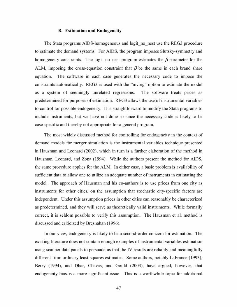
47
B. Estimation and Endogeneity
The Stata programs AIDS-homogeneous and logit_no_nest use the REG3 procedure
to estimate the demand systems. For AIDS, the program imposes Slutsky-symmetry and
homogeneity constraints. The logit_no_nest program estimates the β parameter for the
ALM, imposing the cross-equation constraint that β be the same in each brand share
equation. The software in each case generates the necessary code to impose the
constraints automatically. REG3 is used with the �mvreg� option to estimate the model
as a system of seemingly unrelated regressions. The software treats prices as
predetermined for purposes of estimation. REG3 allows the use of instrumental variables
to control for possible endogeneity. It is straightforward to modify the Stata programs to
include instruments, but we have not done so since the necessary code is likely to be
case-specific and thereby not appropriate for a general program.
The most widely discussed method for controlling for endogeneity in the context of
demand models for merger simulation is the instrumental variables technique presented
in Hausman and Leonard (2002), which in turn is a further elaboration of the method in
Hausman, Leonard, and Zona (1994). While the authors present the method for AIDS,
the same procedure applies for the ALM. In either case, a basic problem is availability of
sufficient data to allow one to utilize an adequate number of instruments in estimating the
model. The approach of Hausman and his co-authors is to use prices from one city as
instruments for other cities, on the assumption that stochastic city-specific factors are
independent. Under this assumption prices in other cities can reasonably be characterized
as predetermined, and they will serve as theoretically valid instruments. While formally
correct, it is seldom possible to verify this assumption. The Hausman et al. method is
discussed and criticized by Bresnahan (1996).
In our view, endogeneity is likely to be a second-order concern for estimation. The
existing literature does not contain enough examples of instrumental variables estimation
using scanner data panels to persuade us that the IV results are reliably and meaningfully
different from ordinary least squares estimates. Some authors, notably LaFrance (1993),
Berry (1994), and Dhar, Chavas, and Gould (2003), have argued, however, that
endogeneity bias is a more significant issue. This is a worthwhile topic for additional

48
research but, absent specific information to the contrary, we believe it is generally
reasonable to treat prices in scanner data as predetermined. In the case studies discussed
in Section V, for example, prices for individual products often remain unchanged for
many weeks on end, while the corresponding shares display variation. This is evidence
of a lack of simultaneous feedback from shares to prices.
C. DG-COMP MSP Excel Menu Commands
The user interacts with three components of DG-COMP MSP. First is a set of
commands that the system adds to the Excel menu bar. Second is a �data input sheet�
that the user creates to specify the inputs to the simulation. Third is the output sheet that
contains the results of the simulation. The software is intended to be �user friendly� and
has a self-documenting internal help file.
The commands are placed onto the Excel menu bar automatically when DG-COMP
MSP starts. They are available under the heading �Merger Simulation� and include
commands to control data input options and to carry out simulation. The tree structure of
the commands is summarized in the following table.
Data Input and Workbook Commands Drop-down Menus Create New Data Input Sheet Select/Change Active DG-COMP MSP � Workbook Data Input Sheet Reset Active Data Input Sheet Simulation Options
Divest Brands PCAIDS Merger Simulation PCAIDS Merger Simulation with Nests Non-Nested Logit Parse Stata Log File Logit Simulation Standard AIDS Parse Stata Log File Define Input Area for AIDS Parameters Reorganize AIDS Parameters AIDS Simulation Help
The user must create a �data input sheet� that contains the basic data to specify the
simulation. This information always includes the industry elasticity of demand, the

49
names of the firms, the names of the brands, and the brand shares. For PCAIDS it is also
necessary to include the brand elasticity for a single brand. For nested PCAIDS it is
necessary to specify the name of the nest for each of brands associated with it. For the
ALM, it is necessary to specify the logit β parameter (or, alternatively, the brand
elasticity for a single brand) and brand unit prices. For the full AIDS it is necessary to
include the matrix of estimated price and expenditure coefficients.
The following pages contain screenshots of the inputs for the different demand
models using the beer case study describe in section V.
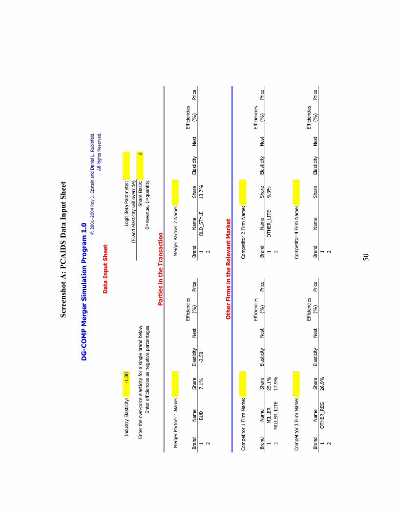
50
Scre
ensh
ot A
: PC
AID
S D
ata
Inpu
t She
et
DG
-CO
MP
Mer
ger
Sim
ulat
ion
Pro
gram
1.0
© 2
001�
2004
Roy
J. E
pste
in a
nd D
anie
l L. R
ubin
feld
.
All R
ight
s R
eser
ved.
Dat
a In
put
She
et
Indu
stry
Ela
stic
ity:
-1.0
0Lo
git Be
ta P
aram
eter
:(B
rand
ela
stic
ity w
ill o
verr
ide)
Ente
r th
e ow
n-pr
ice
elas
ticity
for
a s
ingl
e br
and
belo
w.
Shar
e Ba
sis:
0En
ter
effic
ienc
ies
as n
egat
ive
perc
enta
ges.
0=re
venu
e, 1
=qu
antit
y
Par
ties
in t
he T
rans
acti
on
Mer
ger
Part
ner
1 N
ame:
Mer
ger
Part
ner
2 N
ame:
Bran
dN
ame
Shar
eEl
astic
ityN
est
Effic
ienc
ies
(%)
Pric
eBr
and
Nam
eSh
are
Elas
ticity
Nes
tEf
ficie
ncie
s (%
)Pr
ice
1BU
D7.
1%-2
.50
1O
LD_S
TYLE
13.7
%2
2
Oth
er F
irm
s in
th
e R
elev
ant
Mar
ket
Com
petit
or 1
Firm
Nam
e:Co
mpe
titor
2 F
irm N
ame:
Bran
dN
ame
Shar
eEl
astic
ityN
est
Effic
ienc
ies
(%)
Pric
eBr
and
Nam
eSh
are
Elas
ticity
Nes
tEf
ficie
ncie
s (%
)Pr
ice
1M
ILLE
R25
.1%
1O
TH
ER_L
ITE
9.3%
2M
ILLE
R_L
ITE
17.9
%2
Com
petit
or 3
Firm
Nam
e:Co
mpe
titor
4 F
irm N
ame:
Bran
dN
ame
Shar
eEl
astic
ityN
est
Effic
ienc
ies
(%)
Pric
eBr
and
Nam
eSh
are
Elas
ticity
Nes
tEf
ficie
ncie
s (%
)Pr
ice
1O
THER
_REG
26.9
%1
22

51
Scre
ensh
ot B
: PC
AID
S w
ith N
ests
Dat
a In
put S
heet
DG
-CO
MP
Mer
ger
Sim
ulat
ion
Pro
gram
1.0
© 2
001�
2004
Roy
J. E
pste
in a
nd D
anie
l L. R
ubin
feld
.
All R
ight
s R
eser
ved.
Dat
a In
put
She
et
Indu
stry
Ela
stic
ity:
-1.0
0Lo
git Be
ta P
aram
eter
:(B
rand
ela
stic
ity w
ill o
verr
ide)
Ente
r th
e ow
n-pr
ice
elas
ticity
for
a s
ingl
e br
and
belo
w.
Shar
e Ba
sis:
0En
ter
effic
ienc
ies
as n
egat
ive
perc
enta
ges.
0=re
venu
e, 1
=qu
antit
y
Par
ties
in t
he T
rans
acti
on
Mer
ger
Part
ner
1 N
ame:
Mer
ger
Part
ner
2 N
ame:
Bran
dN
ame
Shar
eEl
astic
ityN
est
Effic
ienc
ies
(%)
Pric
eBr
and
Nam
eSh
are
Elas
ticity
Nes
tEf
ficie
ncie
s (%
)Pr
ice
1BU
D7.
1%-2
.50
reg
1O
LD_S
TYLE
13.7
%re
g2
2
Oth
er F
irm
s in
th
e R
elev
ant
Mar
ket
Com
petit
or 1
Firm
Nam
e:Co
mpe
titor
2 F
irm N
ame:
Bran
dN
ame
Shar
eEl
astic
ityN
est
Effic
ienc
ies
(%)
Pric
eBr
and
Nam
eSh
are
Elas
ticity
Nes
tEf
ficie
ncie
s (%
)Pr
ice
1M
ILLE
R25
.1%
reg
1O
TH
ER_L
ITE
9.3%
lite
2M
ILLE
R_L
ITE
17.9
%lit
e2
Com
petit
or 3
Firm
Nam
e:Co
mpe
titor
4 F
irm N
ame:
Bran
dN
ame
Shar
eEl
astic
ityN
est
Effic
ienc
ies
(%)
Pric
eBr
and
Nam
eSh
are
Elas
ticity
Nes
tEf
ficie
ncie
s (%
)Pr
ice
1O
THER
_REG
26.9
%re
g1
22
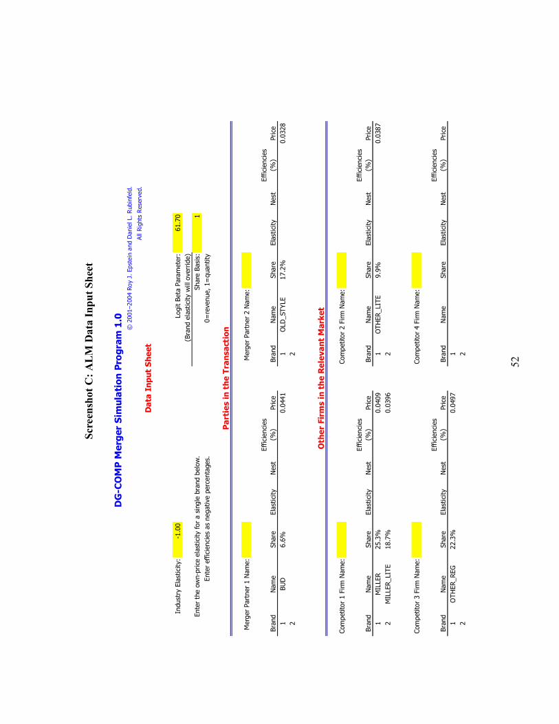
52
Scre
ensh
ot C
: AL
M D
ata
Inpu
t She
et
DG
-CO
MP
Mer
ger
Sim
ulat
ion
Pro
gram
1.0
© 2
001�
2004
Roy
J. E
pste
in a
nd D
anie
l L. R
ubin
feld
.
All R
ight
s R
eser
ved.
Dat
a In
put
She
et
Indu
stry
Ela
stic
ity:
-1.0
0Lo
git Be
ta P
aram
eter
:61
.70
(Bra
nd e
last
icity
will
ove
rrid
e)En
ter
the
own-
pric
e el
astic
ity for
a s
ingl
e br
and
belo
w.
Shar
e Ba
sis:
1En
ter
effic
ienc
ies
as n
egat
ive
perc
enta
ges.
0=re
venu
e, 1
=qu
antit
y
Par
ties
in t
he T
rans
acti
on
Mer
ger
Part
ner
1 N
ame:
Mer
ger
Part
ner
2 N
ame:
Bran
dN
ame
Shar
eEl
astic
ityN
est
Effic
ienc
ies
(%)
Pric
eBr
and
Nam
eSh
are
Elas
ticity
Nes
tEf
ficie
ncie
s (%
)Pr
ice
1BU
D6.
6%0.
0441
1O
LD_S
TYLE
17.2
%0.
0328
22
Oth
er F
irm
s in
th
e R
elev
ant
Mar
ket
Com
petit
or 1
Firm
Nam
e:Co
mpe
titor
2 F
irm N
ame:
Bran
dN
ame
Shar
eEl
astic
ityN
est
Effic
ienc
ies
(%)
Pric
eBr
and
Nam
eSh
are
Elas
ticity
Nes
tEf
ficie
ncie
s (%
)Pr
ice
1M
ILLE
R25
.3%
0.04
091
OTH
ER_L
ITE
9.9%
0.03
872
MIL
LER_L
ITE
18.7
%0.
0396
2
Com
petit
or 3
Firm
Nam
e:Co
mpe
titor
4 F
irm N
ame:
Bran
dN
ame
Shar
eEl
astic
ityN
est
Effic
ienc
ies
(%)
Pric
eBr
and
Nam
eSh
are
Elas
ticity
Nes
tEf
ficie
ncie
s (%
)Pr
ice
1O
THER
_REG
22.3
%0.
0497
12
2

53
Scre
ensh
ot D
: AID
S D
ata
Inpu
t She
et
DG
-CO
MP
Mer
ger
Sim
ulat
ion
Pro
gram
1.0
© 2
001�
2004
Roy
J. E
pste
in a
nd D
anie
l L. R
ubin
feld
.
All R
ight
s R
eser
ved.
Dat
a In
put
She
et
Indu
stry
Ela
stic
ity:
-1.0
0Lo
git Be
ta P
aram
eter
:(B
rand
ela
stic
ity w
ill o
verr
ide)
Ente
r th
e ow
n-pr
ice
elas
ticity
for
a s
ingl
e br
and
belo
w.
Shar
e Ba
sis:
0En
ter
effic
ienc
ies
as n
egat
ive
perc
enta
ges.
0=re
venu
e, 1
=qu
antit
y
Par
ties
in t
he T
rans
acti
on
Mer
ger
Part
ner
1 N
ame:
Mer
ger
Part
ner
2 N
ame:
Bran
dN
ame
Shar
eEl
astic
ityN
est
Effic
ienc
ies
(%)
Pric
eBr
and
Nam
eSh
are
Elas
ticity
Nes
tEf
ficie
ncie
s (%
)Pr
ice
1BU
D7.
1%1
OLD
_STY
LE13
.7%
22
Oth
er F
irm
s in
th
e R
elev
ant
Mar
ket
Com
petit
or 1
Firm
Nam
e:Co
mpe
titor
2 F
irm N
ame:
Bran
dN
ame
Shar
eEl
astic
ityN
est
Effic
ienc
ies
(%)
Pric
eBr
and
Nam
eSh
are
Elas
ticity
Nes
tEf
ficie
ncie
s (%
)Pr
ice
1M
ILLE
R25
.1%
1O
TH
ER_L
ITE
9.3%
2M
ILLE
R_L
ITE
17.9
%2
Com
petit
or 3
Firm
Nam
e:Co
mpe
titor
4 F
irm N
ame:
Bran
dN
ame
Shar
eEl
astic
ityN
est
Effic
ienc
ies
(%)
Pric
eBr
and
Nam
eSh
are
Elas
ticity
Nes
tEf
ficie
ncie
s (%
)Pr
ice
1O
THER
_REG
26.9
%1
22
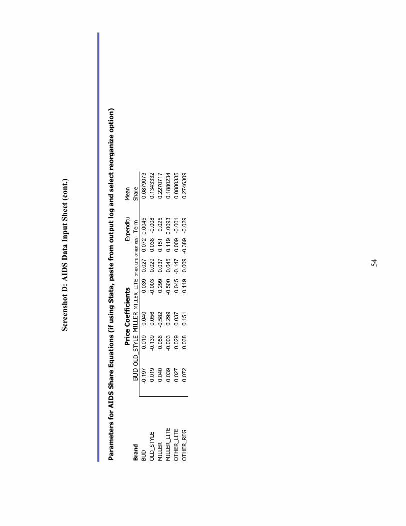
54
Scre
ensh
ot D
: AID
S D
ata
Inpu
t She
et (c
ont.)
Par
amet
ers
for
AID
S Sh
are
Equa
tion
s (i
f u
sin
g S
tata
, pas
te f
rom
ou
tpu
t lo
g an
d se
lect
reo
rgan
ize
opti
on)
Pri
ce C
oeff
icie
nts
Expe
nditu
Mea
nB
ran
dBU
DO
LD_S
TYLE
MIL
LER
MIL
LER_
LITE
OTH
ER_L
ITE
OTH
ER_R
EGTe
rmSh
are
BUD
-0.197
0.019
0.040
0.039
0.027
0.0720.0045
0.0879073
OLD
_STY
LE0.019
-0.139
0.056
-0.003
0.029
0.038-0.008
0.1343332
MIL
LER
0.040
0.056
-0.582
0.299
0.037
0.151
0.025
0.2270717
MIL
LER
_LIT
E0.039
-0.003
0.299
-0.500
0.045
0.1190.0093
0.1880234
OTH
ER_L
ITE
0.027
0.029
0.037
0.045-0.147
0.009-0.001
0.0880335
OTH
ER_R
EG0.072
0.038
0.151
0.119
0.009-0.389
-0.029
0.2746309

55
The menu command �Select/Change Active DG-COMP MSP �� is used to switch
among different input sources. Click on a cell in the desired workbook or data input
sheet and then invoke the command to identify the choice to the software. The selected
workbook or data input sheet is referred to as �active.�
The �Reset Active Data Input Sheet� command clears the data from the active sheet
and restores the default formatting.
The �Divest Brands� command is an option to specify hypothetical divestiture of
one or more brands sold by the merging firms. Each brand can be divested either to an
existing competitor or a hypothetical new entrant. A firm is not permitted to divest all of
its brands. After the divestiture is specified, the actual simulation is carried out by using
one of the following commands.
The �PCAIDS Merger Simulation� command performs PCAIDS simulation and
appends the results to an output worksheet. The output worksheet has the name
datainputsheetname_PCAIDS.
The �PCAIDS Merger Simulation with Nests� command performs PCAIDS
simulation with nests and appends the results to an output worksheet. After this
command is selected, the user is prompted to specify the lower triangle of the
(symmetric) matrix of nesting parameters. The output worksheet has the name
datainputsheetname_NESTED_PCAIDS.
The �Non-Nested Logit� command has submenus to process the Stata log file (when
the logit β parameter is estimated econometrically) and to perform simulation using the
ALM. The simulation results are appended to an output worksheet with the name
datainputsheetname_LOGIT. For further information on processing the Stata file see
section IV.D.2 below.
The �Standard AIDS� command has submenus to process the Stata log file with
AIDS estimation results and to perform simulation using the ALM. The simulation
results are appended to an output worksheet with the name datainputsheetname_AIDS.
For further information on processing the Stata file see section IV.D.1 below.
The �Help� command provides brief descriptions of these menu choices.
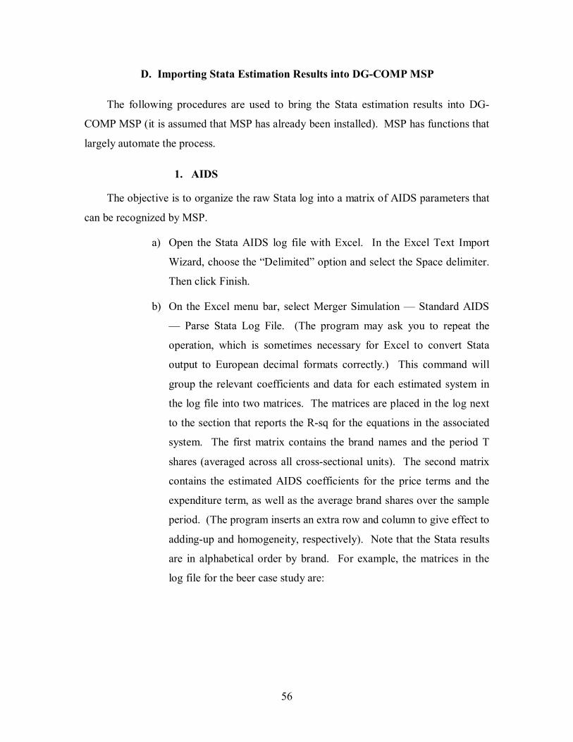
56
D. Importing Stata Estimation Results into DG-COMP MSP
The following procedures are used to bring the Stata estimation results into DG-
COMP MSP (it is assumed that MSP has already been installed). MSP has functions that
largely automate the process.
1. AIDS
The objective is to organize the raw Stata log into a matrix of AIDS parameters that
can be recognized by MSP.
a) Open the Stata AIDS log file with Excel. In the Excel Text Import
Wizard, choose the �Delimited� option and select the Space delimiter.
Then click Finish.
b) On the Excel menu bar, select Merger Simulation � Standard AIDS
� Parse Stata Log File. (The program may ask you to repeat the
operation, which is sometimes necessary for Excel to convert Stata
output to European decimal formats correctly.) This command will
group the relevant coefficients and data for each estimated system in
the log file into two matrices. The matrices are placed in the log next
to the section that reports the R-sq for the equations in the associated
system. The first matrix contains the brand names and the period T
shares (averaged across all cross-sectional units). The second matrix
contains the estimated AIDS coefficients for the price terms and the
expenditure term, as well as the average brand shares over the sample
period. (The program inserts an extra row and column to give effect to
adding-up and homogeneity, respectively). Note that the Stata results
are in alphabetical order by brand. For example, the matrices in the
log file for the beer case study are:

57
Period T Share
BUD 0.071 MILLER 0.251 MILLER_LITE 0.179 OLD_STYLE 0.137 OTHER_LIGHT 0.093 OTHER_REG 0.269
and (note the column without a name contains the price coefficients
obtained by imposing homogeneity)
lnp1
lnp2
lnp3
lnp4
lnp5
lnrexp
Mean Share
�0.197 0.040 0.039 0.019 0.027 0.072 0.004 0.088 0.040 �0.582 0.299 0.056 0.037 0.151 0.025 0.227 0.039 0.299 �0.500 �0.003 0.045 0.119 0.009 0.188 0.019 0.056 �0.003 �0.139 0.029 0.038 �0.008 0.134 0.027 0.037 0.045 0.029 �0.147 0.009 �0.001 0.088 0.072 0.151 0.119 0.038 0.009 �0.389 �0.029 0.275
c) Create an MSP input data sheet in the Excel file by selecting Merger
Simulation � Create New Data Input Sheet. Alternatively, if a data
input sheet already exists, activate it by selecting the appropriate
Merger Simulation command. On the MSP input data sheet, enter the
industry elasticity and the names and shares of the brands for each
firm. The names of the brands must match the names used in Stata. If
the brand shares are based on revenue, enter 0 in the yellow-
highlighted cell M9. Usually, the easiest way to enter the brand names
and shares is to copy the first matrix from the log file and paste it into
a blank area of the input data sheet. Use the mouse to drag each brand
and share to the appropriate area of the input data sheet.
d) Select Merger Simulation � Standard AIDS � Define Input Area for
AIDS Parameters. This will create row and column labels for a blank
matrix.
e) Copy the second matrix created in the AIDS log in step b) and paste
special it into the area created in the input data sheet in step d). Copy
only the numerical values, there should be N rows and N+2 columns,

58
where N is the total number of brands in the analysis. Do not copy the
header row with the column names.
f) Finally, select Merger Simulation � Standard AIDS � Reorganize
AIDS Parameters. This orders the data in the matrix by brand by firm,
as required for the simulation, instead of alphabetically.
If you choose to create the input data sheet in the log file after it was brought into
Excel, be sure to save the log file as a standard Excel workbook without the �.log�
extension in the filename.
The actual simulation is run by selecting Merger Simulation � Standard AIDS �
AIDS Simulation. Note that the estimated fixed effects are not needed for the simulation.
2. Logit
The Stata log provides the brand names, period T average shares and T prices, and
the estimated logit β coefficient.
a) Open the Stata LOGIT log file with Excel. In the Excel Text Import
Wizard, choose the �Delimited� option and select the Space delimiter.
Then click Finish.
b) On the Excel menu bar, select Merger Simulation � Non-Nested
Logit � Parse Stata Log File. (The program may ask you to repeat
the operation, which is sometimes necessary for Excel to convert Stata
output to European decimal formats correctly.) The command will
group the brand names and period T shares and prices at the start of
the log for each estimated system. The command also inserts the
estimated logit β coefficient from the regression output alongside this
information. Note that the Stata results are in alphabetical order by
brand. For example, the log for the beer case study after the parse
command contained:

59
Brand q_shar~T price_T Beta BUD 0.066 0.044 �61.697 MILLER 0.253 0.041 MILLER_LITE 0.187 0.040 OLD_STYLE 0.172 0.033 OTHER_LIGHT 0.099 0.039 OTHER_REG 0.223 0.050
c) Create an MSP input data sheet in the Excel file by selecting Merger
Simulation � Create New Data Input Sheet. Alternatively, if a data
input sheet already exists, activate it by selecting the appropriate
Merger Simulation command. On the MSP input data sheet, enter the
industry elasticity and the names, shares, and prices of the brands for
each firm. Usually, the easiest way to enter the brand names, shares,
and prices is to copy the block of information from the log file and
paste it into a blank area of the input data sheet (omitting the header
row with the column names). Use the mouse to drag each
brand/share/price combination to the appropriate area of the input data
sheet. (Include the 3 blank cells between the share and the price when
dragging to conform to the layout of the data input sheet).
d) Copy the value of the estimated β coefficient and paste special it into
the highlighted cell M7. Make sure that a brand elasticity is not
entered elsewhere on the data input sheet. A brand elasticity, if
specified, implies a value of β that will override the value entered in
M7.
e) If the brand shares are based on quantities, enter 1 in the highlighted
cell M9, else enter 0. The shares in the logit log file should be based
on quantity.
If you choose to create the input data sheet in the log file after it was brought into
Excel, be sure to save the log file as a standard Excel workbook without the �.log�
extension in the filename.
The actual simulation is run by selecting Merger Simulation � Non-Nested Logit
� Logit Simulation. The estimated fixed effects are not needed for the simulation.

60

61
V. CASE STUDIES
We now describe the results of two illustrative case studies. The first study
involves beer and the second toilet tissue. The data were obtained from a public use
database of supermarket scanner data maintained by the University of Chicago. The data
are described in detail at http://www.gsb.uchicago.edu/kilts/research/db/dominicks/. The
complete database contains approximately 9 years of weekly store-level data for the
Dominick�s supermarket chain in the Chicago area, covering sales of more than 3500
UPCs (Universal Product Codes) in several dozen stores. The case studies used a subset
of the available data to simplify management of the input files.
A. Beer
The beer data included weekly observations for approximately 2 years on 186
separate products in 5 stores. The UPCs track products at a very detailed level, e.g., sales
of Beck�s Bier are recorded separately for cans and bottles. Moreover, many of the
UPC�s have very small sales and some even have zero sales in a given week. For
purposes of the case study, the UPCs were aggregated into 6 composite brands:
Budweiser, Miller, Miller Lite, Old Style, Other Light Beer, and Other Regular Beer.
The average shares across the sample stores at the end of the sample were as follows:
Brand
Revenue Share (%)
Quantity Share (%)
BUD 7.1 6.6 MILLER 25.1 25.3 MILLER_LITE 17.9 18.7 OLD_STYLE 13.7 17.2 OTHER_LIGHT 9.3 9.9 OTHER_REG 26.9 22.3 Total 100.0 100.0
The econometric estimation used these brands with fixed effects for each brand for each
of the 5 stores.
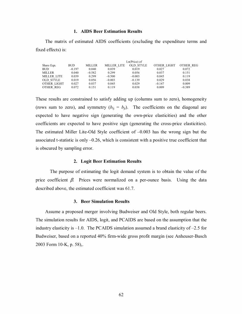
62
1. AIDS Beer Estimation Results
The matrix of estimated AIDS coefficients (excluding the expenditure terms and
fixed effects) is:
Ln(Price) of Share Eqn. BUD MILLER MILLER_LITE OLD_STYLE OTHER_LIGHT OTHER_REG BUD �0.197 0.040 0.039 0.019 0.027 0.072 MILLER 0.040 �0.582 0.299 0.056 0.037 0.151 MILLER_LITE 0.039 0.299 �0.500 �0.003 0.045 0.119 OLD_STYLE 0.019 0.056 �0.003 �0.139 0.029 0.038 OTHER_LIGHT 0.027 0.037 0.045 0.029 �0.147 0.009 OTHER_REG 0.072 0.151 0.119 0.038 0.009 �0.389
These results are constrained to satisfy adding up (columns sum to zero), homogeneity
(rows sum to zero), and symmetry (bij = bji). The coefficients on the diagonal are
expected to have negative sign (generating the own-price elasticities) and the other
coefficients are expected to have positive sign (generating the cross-price elasticities).
The estimated Miller Lite-Old Style coefficient of �0.003 has the wrong sign but the
associated t-statistic is only �0.26, which is consistent with a positive true coefficient that
is obscured by sampling error.
2. Logit Beer Estimation Results
The purpose of estimating the logit demand system is to obtain the value of the
price coefficient β. Prices were normalized on a per-ounce basis. Using the data
described above, the estimated coefficient was 61.7.
3. Beer Simulation Results
Assume a proposed merger involving Budweiser and Old Style, both regular beers.
The simulation results for AIDS, logit, and PCAIDS are based on the assumption that the
industry elasticity is �1.0. The PCAIDS simulation assumed a brand elasticity of �2.5 for
Budweiser, based on a reported 40% firm-wide gross profit margin (see Anheuser-Busch
2003 Form 10-K, p. 58),.

63
Simulation Method
Brand
Predicted Unilateral Effect (%)
AIDS BUD 3.4 OLD_STYLE 3.0 Logit BUD 6.0 OLD_STYLE 1.5 PCAIDS BUD 4.5 OLD_STYLE 2.5
Note that the logit simulation yields the highest single effect, as well as the lowest effect.
Alternatively, for the PCAIDS analysis one might expect that regular beer and light
beer should be in separate nests. The following simulation assumes a nesting parameter
equal to 0.25, implying that light beer is a poor substitute for regular beer.
Simulation Method
Brand
Predicted Unilateral Effect (%)
NESTED PCAIDS BUD 6.1 OLD_STYLE 3.5
The predicted effects are somewhat larger compared to the non-nested PCAIDS. Note
that the nest structure effectively makes the pre-merger market more concentrated with
respect to Budweiser and Old Style because they are both regular beers. The light beers
nest has less ability to constrain the effect of the merger.
B. Toilet Tissue
The toilet tissue data included weekly observations for approximately 2 years on 110
separate products in 4 stores. These products often have minimal differentiation, e.g.,
sales for a given manufacturer can be recorded separately depending on the color of the
tissue. As with beer, some UPC�s had very small and even zero sales in a given week.
For the case study, the UPCs were aggregated into 5 composite brands: Charmin,
Kleenex, Northern, Scott, and Other.
The average shares across the stores at the end of the estimation period were as
follows:

64
Brand
Revenue Share (%)
Quantity Share (%)
CHARMIN 21.9 22.5 KLEENEX 24.1 19.8 NORTHERN 16.8.0 21.0 OTHER 11.7 17.8 SCOTT 25.5 18.9 TOTAL 100.0 100.0
The econometric estimation used these brands with fixed effects for each brand for each
of the 4 stores. Note that the revenue share for Scott is much larger than its quantity
share. A difference of this magnitude is likely to result in significantly larger unilateral
effects in the AIDS framework. It should be noted, however, that the quantity share is
given (as reported) in terms of rolls of paper. Casual inspection at the supermarket
reveals that Scott has many more sheets per roll than other brands, so the Scott quantity
share would be underestimated if number of sheets is the more appropriate unit of
measurement.
1. AIDS Tissue Estimation Results
The matrix of estimated AIDS coefficients (excluding the expenditure terms and
fixed effects) is:
Ln(Price) of Share Eqn. CHARMIN KLEENEX NORTHERN OTHER SCOTT CHARMIN �0.575 0.092 0.150 0.098 0.236 KLEENEX 0.092 �0.500 0.177 0.086 0.145 NORTHERN 0.150 0.177 �0.777 0.128 0.322 OTHER 0.098 0.086 0.128 �0.360 0.048 SCOTT 0.236 0.145 0.322 0.048 �0.751
The estimation imposes the same constraints of adding-up, homogeneity, and symmetry.
All of the estimated coefficients have the expected sign.
2. Logit Tissue Estimation Results
The purpose of estimating the logit demand system is to obtain the value of the price
coefficient β. Prices were normalized on a per roll basis. It is known that sheets per roll
vary across brands, indicating it might be more appropriate to normalize on a per sheet
basis. However, data on number of sheets per roll were not available. Using the data
described above, the estimated coefficient was 9.12.
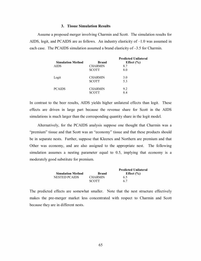
65
3. Tissue Simulation Results
Assume a proposed merger involving Charmin and Scott. The simulation results for
AIDS, logit, and PCAIDS are as follows. An industry elasticity of �1.0 was assumed in
each case. The PCAIDS simulation assumed a brand elasticity of �3.5 for Charmin.
Simulation Method
Brand
Predicted Unilateral Effect (%)
AIDS CHARMIN 8.7 SCOTT 8.0 Logit CHARMIN 3.0 SCOTT 5.3 PCAIDS CHARMIN 9.2 SCOTT 8.4
In contrast to the beer results, AIDS yields higher unilateral effects than logit. These
effects are driven in large part because the revenue share for Scott in the AIDS
simulations is much larger than the corresponding quantity share in the logit model.
Alternatively, for the PCAIDS analysis suppose one thought that Charmin was a
�premium� tissue and that Scott was an �economy� tissue and that these products should
be in separate nests. Further, suppose that Kleenex and Northern are premium and that
Other was economy, and are also assigned to the appropriate nest. The following
simulation assumes a nesting parameter equal to 0.5, implying that economy is a
moderately good substitute for premium.
Simulation Method
Brand
Predicted Unilateral Effect (%)
NESTED PCAIDS CHARMIN 6.5 SCOTT 6.7
The predicted effects are somewhat smaller. Note that the nest structure effectively
makes the pre-merger market less concentrated with respect to Charmin and Scott
because they are in different nests.

66
C. Business Software
In a recent case, the U.S. brought suit against Oracle Corporation, alleging that the
proposed hostile acquisition of PeopleSoft by Oracle is anticompetitive and violates
Section 7 of the Clayton Act. The District Court ruled against the U.S., but as this is
written, it appears likely that the decision of the Court will be appealed. Whatever the
ultimate outcome, the case raises interesting questions concerning unilateral effects
analysis generally, and merger simulation and geographic market definition specifically.
In what follows, we briefly highlight some of those questions.40
According to the Department of Justice, Oracle, PeopleSoft, and SAP are the only
three firms in a $500 million U.S. market for high function business applications software
(i.e., software sold to major businesses to manage their operations). DOJ argued that the
merger is 3-to-2 in that market and will lessen competition. In particular, DOJ alleged
the merging parties have a 48% share in �high function financial management software�
(�FMS�) and a 68% share in �high function human resource management software�
(�HRM�). Oracle countered that these shares were overstated because the geographic
market should include at least Europe and perhaps the rest of the world, and that the
product market is too narrow. The parties also disagreed as to the extent, if any, of the
unilateral effects that will be generated as the result of the merger.41 DOJ claimed that
software prices would increase. Oracle argued they would not, claiming the absence of
significant barriers to entry into DOJ�s alleged product market. In particular, Oracle
pointed to a number of potential competitors, including Microsoft and Lawson, and
argued that customers can protect against any exercise of market power by Oracle by
outsourcing or by obtaining software from potential competitors that are able to
reposition themselves to compete with Oracle and PeopleSoft.
The DOJ submitted economic testimony with respect to market definition (Prof.
Kenneth Elzinga) and unilateral effects (Prof. Preston McAfee). Oracle offered counter
economic testimony on each (by Profs. Jerry Hausman and Tom Campbell, respectively). 40 Redacted versions of the submissions by both parties are available on their respective websites:
www.usdoj.gov/atr/cases, and www.oracle.com/peoplesoft. For a PeopleSoft point of view, see www.peoplesoft.com/corp/en/news_events/news/justice.jsp.
41 Both parties appear to agree that a coordinated effects theory is not appropriate in this case.

67
Oracle�s third economic expert, Prof. David Teece, testified that the market was dynamic
and that the introduction of a new �infrastructure layer� of competitive products marked a
paradigm shift that needed to be accounted for in defining a relevant market.
Judge Walker ruled for Oracle in his September 2004 decision. In Judge Walker�s
opinion, the U.S. did not meet its legal burden to prove by a preponderance of the
evidence that (i) HRM and FMS (both forms of high function software) define separate
relevant product markets; (ii) the relevant geographic market is the U.S. as opposed to a
world market; (iii) there are any significant unilateral effects. The Court also ruled that
Oracle had not proved any efficiencies, but that point will be moot unless the District
Court�s opinion is overturned and the case is remanded for further proceedings.
The Oracle case raises two issues that are relevant for this Report. The first one
concerns which empirical methods for evaluating unilateral effects are relevant in an
auction situation in which many contracts are put up for bid. The second involves
application of the Elzinga-Hogarty test. We discuss each of these issues, in reverse order.
1. Geographic Market
With respect to geographic market definition, DOJ (citing the Horizontal Merger
Guidelines) argued that the scope of the market is the U.S. because �there was no
evidence that [U.S. customers] could effectively turn outside of [the United States] for
alternative sources of [the product.]42 The government argued further that customers are
business units operating in the U.S., wherever their corporate headquarters might be
located. Prof. Elzinga testified that licensing high function software involves on-going
customer relationships that require on-site evaluations and demonstrations, as well as
product support and continuing maintenance and upgrades. Such relationships, he
argued, necessitate a vendor with significant domestic operations. He testified further
that, because arbitrage is not possible, a hypothetical monopolist of U.S. sales of the
product could raise prices in the U.S. (the price increase would not be defeated by
importation). Ironically, Prof. Elzinga rejected the application of an Elzinga-Hogarty test
in this case because the test �was designed for product markets that are literally shipped
42 DOJ, Post-trial Brief, July, 2004. p.23.

68
from factory to customer, that have substantial transportation costs relative to the value of
the product, and for which there are no legal impediments to shipment across geographic
boundaries.�43 He also argued that the Elzinga-Hogarty test should not be applied to the
case due to the existence of geographic price discrimination.
Oracle claimed the geographic market is worldwide and that if there were a U.S.
market, Oracle does not have significant market power because market shares should
�reflect global capabilities � because SAP�s dominance globally, and in particular
among global enterprises, would be enough to defeat plaintiffs� claims.�44 Oracle argued
further for a worldwide market using four distinct �tests:�45 (1) sellers such as SAP,
Oracle, PeopleSoft, Siebel, and Microsoft market their software globally; (2) the Elzinga-
Hogarty test indicates a worldwide market; (3) software transportation costs are minimal;
and (4) prices in the U.S. tend to move uniformly with prices outside the U.S. (relying on
the Stigler-Sherwin test and an empirical analysis of Prof. Hausman).
The Court rejected Prof. Elzinga�s argument that the geographic marked is limited
by the fact that products are marketed and supported in the U.S. The Court also
concluded that an Elzinga-Hogarty test was appropriate in this case, from which it
follows that the relevant geographic market is worldwide.46 Nevertheless, the testimony
by both sides confirms that there is no single best test to determine a relevant market, and
that good economics involves a judicious evaluation of a range of documentary and
empirical evidence as well as the choice of an appropriate methodology.
2. Unilateral Effects
DOJ argues that by eliminating PeopleSoft as a competitor, the proposed acquisition
would cause Oracle to offer lower discounts to U.S. customers on its high function
business software. The Government identifies four distinct unilateral effects theories,
namely mergers that will raise price by:
43 Id., p. 24. 44 Oracle, Post-trial Brief, July, 2004, p. 22 45 Id., p. 23�24. 46 Opinion of the District Court, pp. 132-136.

69
�(a) creating a monopoly or dominant firms; (b) perpetuating a monopoly or dominant firm by eliminating a nascent rival; (c) giving one firm stronger control of its �niche� in a product-differentiated market; or (d) strengthening a firm�s power to make noncompetitive bids that buyers will be unable to refuse.�47
DOJ argued that points (c) and (d) apply to this case. In response to a challenge by Judge
Walker, DOJ pointed in particular to the analysis of unilateral effects in FTC v. Swedish
Match and to FTC v. Staples, Inc.48 and cited legal commentator Herbert Hovenkamp:
�Unilateral effects theories have proven to be among the most useable and robust contributions of the post-Chicago revolution in antitrust economics � Unilateral effects methodologies for analyzing mergers must be regarded as, if anything, more reliable than the methodologies used for evaluating mergers under the traditional concerns about increased concentration.�49
In support of its unilateral effects case, DOJ cited documentary evidence and offered
direct testimony from customers that Oracle and PeopleSoft are each others� closest
competitors. Prof. McAfee emphasized that competition in this market involves a
customer-specific bidding process. Prof. McAfee relied on three separate analyses to
conclude that there will be significant price effects in the relevant market: (1) an analysis
of 25 specific cases of competition between Oracle and PeopleSoft; (2) a regression
analysis showing that when PeopleSoft is a competitor, Oracle offers higher discounts;
and (3) a more general analysis of bidding behavior using auction theory. All three
analyses led Prof. McAfee to conclude that the proposed merger will result in higher
prices.
In response, Oracle argued that it will not be able to raise prices post-merger. Citing
the Guidelines presumption that unilateral effects are not likely to be a problem if the
post-merger market share of the firm is less than 35%, Oracle used product and
geographic market definitions to support its view that the post-merger share will be
47 DOJ, Post-trial Brief, p. 28. 48 131 F. Supp. 2d 151 (D.D.C. 2000) and 970 F. Supp. 1066 (D.D.C. 1997), respectively. These were
cases in which the Government as successful. The defendant was victorious in a number of other unilateral effects cases, including U.S. v. Long Island Jewish Med. Ctr. (983 F. Supp. 121 at 142�144) and NewYork v. Kraft Gen. Foods (926 F. Supp. 321 at 352�33).
49 Herbert Hovenkamp, �Post-Chicago Antitrust: a Review and Critique,� 2001 Colum. Bus. L. Rev. 257, 333.
70
significantly less than 35%. Oracle argued further that market shares are likely to give an
inaccurate picture of this acquisition since (1) customers choose to limit the number of
vendors, they do not care to have a large number of bidders; and (2) it is difficult to
predict price effects in markets in which buyers as well as sellers have substantial market
power.
Finally, Oracle argued that an appropriate unilateral effects analysis of the diversion
of sales requires extensive econometric analysis and that DOJ failed to provide one.
Interestingly, Oracle pointed explicitly to the potential of merger simulation as a valuable
tool. Oracle�s position, however, was that the relevant demand elasticities should be
estimated econometrically and should not be based on qualitative assessments. Oracle
also criticized Profs. Elzinga and McAfee for assuming closeness of products based on
market shares, without developing appropriate evidentiary support.
In ruling for Oracle, Judge Walker placed a significant burden on the DOJ.
According to Judge Walker, �to prevail on a differentiated products unilateral effects
claim, a plaintiff must prove a relevant market in which the merging parties would have
essentially a monopoly or dominant position.�50 In Judge Walker�s view, DOJ�s customer
testimony was not sufficient to support the Government�s market definition. As a result,
he rejected the DOJ alleged market shares as inapplicable.51
Judge Walker also concluded that the Government failed to prove that Oracle and
PeopleSoft were each others� closest competitor. He rejected the testimony of Prof.
McAfee on unilateral effects because that testimony was based on the wrong market
definition (a U.S. rather than global market). Judge Walker also criticized the
Government (and its expert Prof. Elzinga) for not presenting market definition testimony
based on econometric analyses of cross-price elasticities and/or diversion ratios.
50 District Court Opinion, p. 47. 51 District Court Opinion, p. 140.

71
VI. TECHNICAL APPENDIX
This appendix has two main purposes. First, it presents the specification of the
ALM and AIDS econometric demand models used by the Stata programs. Second, it
allows a user of the simulation software to follow the calculations and verify the solution.
Because it is intended to be a complete, stand-alone explanation, it may repeat
information presented elsewhere in this Report. We provide examples to illustrate the
details of the calculations for each of the four simulation models.
A. Notation
The following notation is used throughout the Appendix. There are n firms. Each
firm produces ni brands, for a total of N brands. All brands are �inside� goods. There are
I �cities� and T time periods in the data.
The kth brand has the following characteristics:
qkit � brand quantity sold in city i during period t. pkit � brand price in city i during period t.
skit � brand share in city i during period t. The share is based on quantity for ALM and is based on revenue for AIDS and PCAIDS.
εkk � own-price elasticity
εjk � cross-price elasticity of brand j with respect to change in price of brand k
ck � incremental cost (assumed constant)
µk = average brand profit margin (pk � ck)/pk. In addition, we require:
Ei � transposed matrix of own-price and cross-price elasticities for the ith firm, with element (k, j) equal to εjk.
γk � merger-specific efficiency for the kth brand, i.e., ckpost = (1 + γk)ck.
δki � fixed effect for brand k, city i xit � total nominal expenditure in city i during period t for the brands
represented by s1�sN. Pit � a price index

72
ε � industry elasticity of demand
B. Econometric Estimation
1. ALM
The dependent variables for the regressions in the ALM are constructed by taking
logarithmic transformations of the share data, which yields a convenient linear model.
One brand is used as a numeraire good, so the estimated model contains only N�1 brand
share equations. Without loss of generality, brand N is used as a numeraire. The logit
model implies that the observed market shares satisfy
∑ ++
=)exp(
)exp(
jitj
kitkkit p
ps
βαβα
.
where β and the α�s are parameters to be determined. The model is linearized by using
the transformation ln(skit/sNit) as the dependent variable for the brand k share equation.
After the transformation, each brand share equation is of the form
ln(skit / sNijt) = αk � αN + β(pkit � pNit).
Because this is a panel model, it is appropriate to add fixed effects for each brand for
each city. There are therefore I�1 fixed effects (to avoid perfect collinearity) per brand.
The complete model can be written as
∑
∑
−
=−−−−−
−
=
++−+=
++−+=
1
1,1,1,11,1
1
1
11111
)()/ln(
)()/ln(
I
mitNmNNititNNNititN
it
I
mmNititNitit
uppss
uppss
δβγ
δβγ
K
Because the underlying theory assumes that β is the same in each equation, the model
should be estimated with a systems estimation procedure to impose the appropriate cross-
equation constraints. If data are available, the user may add additional variables to the

73
system to control for factors other than price. For example, in the context of supermarket
data, the system could include a dummy variable that takes on the value 1 if the brand
was under promotion in a particular time period and 0 otherwise.
2. AIDS
The estimated share equations are of the form skit = ak + ∑bkmln pmit + hkln (xit / Pit)
+ ∑δkj. That is, as a panel model, the brand share equations include I�1 city fixed effects
in addition to the usual price terms and real expenditure term. Because the shares are
defined to add to 100% for each time period in each city, it is appropriate to impose this
�adding up� constraint on the estimation procedure. This is accomplished by estimating
only N�1 share equations for each city and time period. The last equation is obtained as a
residual where sNit is calculated as 1 minus the sum of the other brand shares for the ith
city in each period, which ensures that the constraint is satisfied. We deflate expenditure
using a Stone price index, i.e., ln Pij = ∑ωklnpkij.52 Each weight ωk equals the average
brand k revenue share over the entire sample period. There are therefore I�1 fixed effects
(again, to avoid perfect collinearity). The complete model can then be written as the N�1
equation system:
+++++=
+++++++=
−−−−−
−
=∑
)ln()ln()ln(
)/ln()ln()ln()ln(
,122,111,11,1
1
1
111121211111
NitNNitNitNNitN
it
I
mmititNitNititit
pbpbpbas
uPxhpbpbpbas
K
K
K δ
itN
I
mmNititN uPxh ,1
1
1,11 )/ln( −
−
=−− ++∑δ
Slutsky-symmetry imposes the constraints bij = bji. In addition, the homogeneity
constraint from economic theory is imposed by dropping the ln(pN) term during
estimation (this constraint is testable econometrically). The coefficient biN in the ith
equation is recovered as a residual defined as the negative of the sum of the other b�s in
the equation. As with the ALM, if data are available the user may add additional
52 The formal derivation AIDS requires a trans-log price index but Deaton and Muellbauer (1980, p. 316)
suggested use of Stone�s index as a convenient simplification to linearize the model. The resulting specification is sometimes referred to in the literature as LA/AIDS (�linear approximate AIDS�).

74
variables to the system, such as a dummy variable for brand promotion, to control for
factors other than price and expenditure.
C. Shares and Elasticities for the Simulation Models
We summarize here the determination of shares and elasticities for the demand
models analyzed in this Report.
1. ALM
Elasticities in the ALM depend on two parameters. Typically, the parameters are
the pre-merger industry elasticity ε and the logit parameter β. Let pbar be the (quantity)
share-weighted average price, ∑sipi. The ALM elasticities are53
εj = [β pbar(1 � sj) + εsj] pj / pbar
εjk = sk (�β pbar + ε] pk / pbar .
The prices in these formulas are typically average prices for the entire sample in the
period just prior to the merger. The IIA property holds because εjk = εik. The sign
convention is β < 0, ε < 0, εj < 0, εjk.>0.
Alternative calibrations are possible. For example, suppose exogenous information
was available on ε and one of the brand elasticities εi (instead of β). Given the prices and
shares, one can invert the elasticity formula for εi to solve for β and then calculate the
remaining elasticities in the system.
Higher post-merger prices imply changes in the shares and elasticities. The
calibration of the ALM to produce updated shares is achieved as follows (see Werden and
Froeb, 1994). Define z = ε /(β pbar) using pre-merger information. In addition, for the
kth brand use the average pre-merger share to define αk = ln(sk) � (β pbar) + ln((1�z)/z),
k=1�N. The α�s calculated in this way take account of the averaged data used for the
simulation. The shares are then given by
53 Werden and Froeb (1994), p. 410.

75
∑ ++
=)exp(
)exp(
jj
kkk p
ps
βαβα
.
Werden and Froeb (1994) also show that
∑ ++=
)exp(1 kk ppbar
βαβε .
The post-merger industry elasticity therefore also changes as pbar changes.
2. AIDS
The AIDS elasticities depend on the estimated coefficients from the AIDS model
plus an exogenous value for the industry elasticity. The specific formulas are54
εj = (bjj + εωjhj)/sj �1 + ωj(1+ε )
εjk = (bjk + εωkhj)/sj + ωk(1+ε)
The AIDS elasticities do not involve prices explicitly. Conventionally, the industry
elasticity is assumed to remain constant. The weights ω are the average shares across
cities for the entire sample period. The (revenue) shares s are typically the average shares
at the end of the sample period.
Post-merger shares to calculate post-merger elasticities are calculated as follows.
The AIDS share equation for the ith brand is si = ai + ∑bijlnpj + hiln(x/P). The post-
merger share equals si + dsi. Now, differentiate the share equation totally to set dsi =
∑bijdpj/pj + hiε∑ωjdpj/pj. The second term in this expression makes use of the equations
dx/x = (1+ε)dP/P and dP/P = ∑ωjdpj/pj.
3. PCAIDS
PCAIDS elasticities also depend on two parameters. Typically, the parameters are
the pre-merger industry elasticity ε and one of the brand elasticities. Assume that a value
is available for ε1. Then the entire set of elasticities for the market is given by55
54 Hausman and Leonard (2002), p. 250.
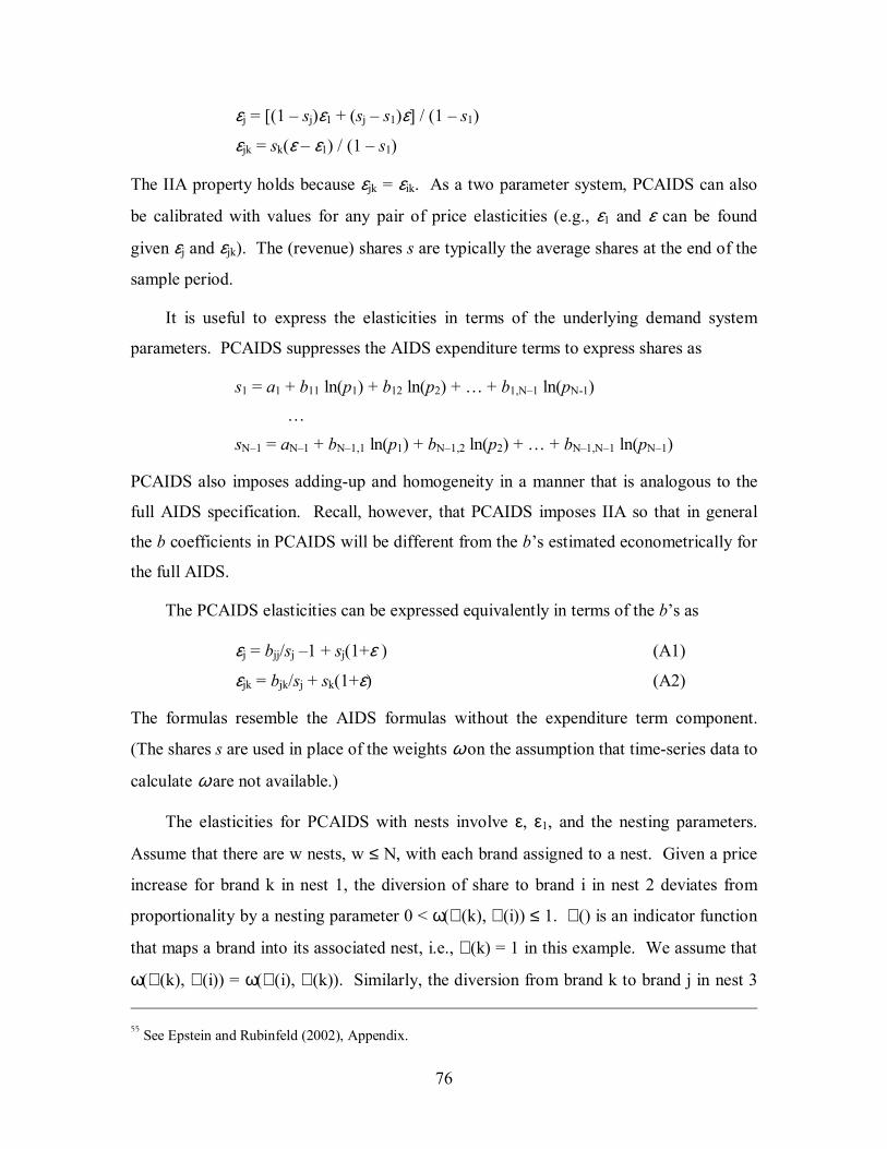
76
εj = [(1 � sj)ε1 + (sj � s1)ε] / (1 � s1)
εjk = sk(ε � ε1) / (1 � s1)
The IIA property holds because εjk = εik. As a two parameter system, PCAIDS can also
be calibrated with values for any pair of price elasticities (e.g., ε1 and ε can be found
given εj and εjk). The (revenue) shares s are typically the average shares at the end of the
sample period.
It is useful to express the elasticities in terms of the underlying demand system
parameters. PCAIDS suppresses the AIDS expenditure terms to express shares as
s1 = a1 + b11 ln(p1) + b12 ln(p2) + � + b1,N�1 ln(pN-1) �
sN�1 = aN�1 + bN�1,1 ln(p1) + bN�1,2 ln(p2) + � + bN�1,N�1 ln(pN�1)
PCAIDS also imposes adding-up and homogeneity in a manner that is analogous to the
full AIDS specification. Recall, however, that PCAIDS imposes IIA so that in general
the b coefficients in PCAIDS will be different from the b�s estimated econometrically for
the full AIDS.
The PCAIDS elasticities can be expressed equivalently in terms of the b�s as
εj = bjj/sj �1 + sj(1+ε ) (A1)
εjk = bjk/sj + sk(1+ε) (A2)
The formulas resemble the AIDS formulas without the expenditure term component.
(The shares s are used in place of the weights ω on the assumption that time-series data to
calculate ω are not available.)
The elasticities for PCAIDS with nests involve ε, ε1, and the nesting parameters.
Assume that there are w nests, w ≤ N, with each brand assigned to a nest. Given a price
increase for brand k in nest 1, the diversion of share to brand i in nest 2 deviates from
proportionality by a nesting parameter 0 < ω(ℑ (k), ℑ (i)) ≤ 1. ℑ () is an indicator function
that maps a brand into its associated nest, i.e., ℑ (k) = 1 in this example. We assume that
ω(ℑ (k), ℑ (i)) = ω(ℑ (i), ℑ (k)). Similarly, the diversion from brand k to brand j in nest 3 55 See Epstein and Rubinfeld (2002), Appendix.
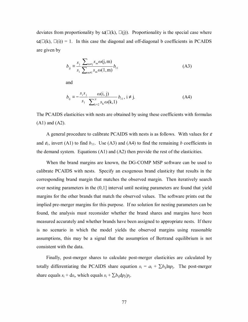
77
deviates from proportionality by ω(ℑ (k), ℑ (j)). Proportionality is the special case where
ω(ℑ (k), ℑ (i)) = 1. In this case the diagonal and off-diagonal b coefficients in PCAIDS
are given by
111m m
jm m
1
jjj m)(1,
m)(j,b
ωs
ωs
ss
b∑∑
≠
≠= (A3)
and
11
2k k1
jiij
(k,1)
j)(i,b
ωs
ωsss
b N∑ =
−= , i ≠ j. (A4)
The PCAIDS elasticities with nests are obtained by using these coefficients with formulas
(A1) and (A2).
A general procedure to calibrate PCAIDS with nests is as follows. With values for ε
and ε1, invert (A1) to find b11. Use (A3) and (A4) to find the remaining b coefficients in
the demand system. Equations (A1) and (A2) then provide the rest of the elasticities.
When the brand margins are known, the DG-COMP MSP software can be used to
calibrate PCAIDS with nests. Specify an exogenous brand elasticity that results in the
corresponding brand margin that matches the observed margin. Then iteratively search
over nesting parameters in the (0,1] interval until nesting parameters are found that yield
margins for the other brands that match the observed values. The software prints out the
implied pre-merger margins for this purpose. If no solution for nesting parameters can be
found, the analysis must reconsider whether the brand shares and margins have been
measured accurately and whether brands have been assigned to appropriate nests. If there
is no scenario in which the model yields the observed margins using reasonable
assumptions, this may be a signal that the assumption of Bertrand equilibrium is not
consistent with the data.
Finally, post-merger shares to calculate post-merger elasticities are calculated by
totally differentiating the PCAIDS share equation si = ai + ∑bijlnpj. The post-merger
share equals si + dsi, which equals si + ∑bijdpj/pj.

78
D. First-Order Conditions for Simulation
1. Pre-Merger
An example with 3 firms is sufficient to illustrate the structure of the first-order
conditions (�FOC�) for the simulation models treated in this Report. Assume that firm 1
produces two brands and that firms 2 and 3 each produce a single brand, for a total of
four brands in the relevant market. We assume a pre-merger equilibrium under static
Bertrand assumptions with constant incremental costs. A firm maximizes profits by
varying its prices under the assumption that its competitors� prices remain fixed. That is,
it solves ∂[∑(pj�cj)qj]/∂pk = 0 for each of the brands it produces.
For a single brand firm, the FOC is 1 � (pk�ck) ∂qk/∂pk = 0. Let PQ represent total
market revenue. It is convenient to multiply both sides of the equation by sk = pkqk / PQ
to express the first-order condition as
sk + skεkkµk = 0 .
This formulation of the FOC is in terms of revenue shares (even if the demand model is
the ALM). A multi-brand firm maximizes profits by taking account of the cross-price
elasticity involving the brands it produces. The number of its first-order conditions
equals the number of its brands. There is a separate first-order condition for each brand
in the market. When the elasticities are known then the pre-merger margins can be
inferred from the first-order conditions.
The set of pre-merger FOCs for the example is
(Firm 1) Brand 1: s1 + s1ε11µ1 + s2ε21µ2 = 0 .
(Firm 1) Brand 2: s2 + s1ε12µ1 + s2ε22µ2 = 0
(Firm 2) Brand 3: s3 + s3ε33µ3 = 0
(Firm 3) Brand 4: s4 + s4ε44µ4 = 0
A general matrix expression for all of the FOCs for all of the brands in the market is
given by
s + diag(E1, E2, …, En)Sµ = 0. (A5)

79
Recall that Ei is an ni by ni matrix of transposed price elasticities for the ith firm. In
equation (A5), s = (s1, s2,… sN)´ is the vector of market shares (in terms of revenue) and S
= diag(s). The corresponding vector of brand margins is µ = (µ1, µ2, …, µN)´. Given the
elasticities and shares, the brand margins µ in the pre-merger equilibrium are given by
µ = � S�1diag(E1, E2,…, En)�1s.
2. Post-Merger
Suppose firms 1 and 2 merge to form NewCo. There are still four first-order
conditions because the number of brands has not changed. However, post-merger there
will be only two firms. The newly merged firm maximizes a new profit function
involving all of the brands it now produces. The new first order conditions are:
(NewCo) Brand 1: s1 + s1ε11µ1 + s2ε21µ2 + s3ε31µ3 = 0 .
(NewCo) Brand 2: s2 + s1ε21µ1 + s2µ2ε22 + s3ε32µ3 = 0
(NewCo) Brand 3: s3 + s1ε31µ1 + s2ε32µ2 + s3ε33µ3 = 0
(Firm 3) Brand 4: s4 + s4ε44µ4 = 0
NewCo has to take account of all of the cross-price elasticities between its products to
maximize profits. The structure of the FOC for firm 3 does not change.
NewCo is characterized by an augmented elasticity matrix E* for the n1 + n2 brands it
is now producing. The general matrix expression for all of the FOCs in the post-merger
market is
s + diag(E*, E3,…, En )Sµ = 0,
where all variables are understood to be taken at their post-transaction values.
Provided the cross-price elasticities are positive so that the goods are substitutes,
NewCo has the unilateral incentive to raise its prices. The new cross-price elasticity
terms imply that its FOCs are positive at pre-merger prices (they had been equal to zero
and the new cross-price term is greater than zero). By raising the brand price, the margin

80
increases and gives greater weight to the negative own-price elasticity, thereby bringing
the FOC back to zero.
Define the percentage changes in the brand prices (e.g., dpi/pi) as the unilateral
effects from the merger. The new prices generated by the unilateral effects give rise to
new margins and shares, which in turn generate new elasticities. The changes in the
shares and elasticities are determined by the demand model, e.g., ALM, AIDS, or
PCAIDS. The solution of the post-merger FOCs is obtained by optimizing with respect
to the vector of unilateral effects.
We calculate the post-merger price for the ith brand as pipost = pi(1+ dpi/pi) in the
ALM and pipost = piexp(dpi/pi) for AIDS and PCAIDS.56 The post-merger margin µi
post =
(pipost � ci
post)/pipost can be parameterized directly in terms of the unilateral effect and the
exogenous efficiency. In particular, µipost = 1 � (1 � µi)(1+γi)/(1 + dp1/p1) for the ALM
and µipost = 1 � (1 � µi)(1+γi)/exp(dp1/p1) for AIDS and PCAIDS.
The calculation of post-merger shares and elasticities for use in the FOCs was
discussed in Section C above.
E. Solution Examples
We use the beer case study to illustrate the calculations underlying simulations with
the alternative demand models used in this Report.
1. ALM
The logit beer analysis is based on the following data:
Brand
Quantity Share (%)
Price ($)
BUD 6.6 0.0441 MILLER 25.3 0.0409 MILLER_LITE 18.7 0.0396 OLD_STYLE 17.2 0.0328 OTHER_LIGHT 9.9 0.0387 OTHER_REG 22.3 0.0497
56 The difference reflects the fact that AIDS and PCAIDS are formulated in terms of the logarithm of
prices.

81
The average price pbar is equal to 0.0412. The estimated β is �61.7. The industry
elasticity was set to �1.0.
DG-COMP MSP reports the following pre-merger matrix of ALM elasticities:
BUD OLD_STYLE MILLER MILLER_LITE OTHER_LITE OTHER_REG BUD �2.61 0.21 0.39 0.28 0.14 0.42 OLD_STYLE 0.11 �1.81 0.39 0.28 0.14 0.42 MILLER 0.11 0.21 �2.14 0.28 0.14 0.42 MILLER_LITE 0.11 0.21 0.39 �2.17 0.14 0.42 OTHER_LITE 0.11 0.21 0.39 0.28 �2.24 0.42 OTHER_REG 0.11 0.21 0.39 0.28 0.14 �2.65
These values match the results of using the formulas in section C.1.. For example, the
own-price elasticity of Miller_Lite is �2.17 = (�61.7(.0412)(1�.187) + (�1)
(.187)).0396/.0412. The software also reports pre-merger margins as:
Brand Margin BUD 0.3830 OLD_STYLE 0.5515 MILLER 0.5421 MILLER_LITE 0.5557 OTHER_LITE 0.4453 OTHER_REG 0.3769
To evaluate the FOCs as we have expressed them, the quantity shares in the ALM need to
be converted to revenue shares. This is accomplished by rescaling si′ = pisi/pbar, where si
is the quantity share.
The pre-merger FOCs are satisfied with the calculated shares, elasticities, and
margins. For example, the rescaled revenue shares for Miller and Miller Lite are 25.09%
and 17.91%, respectively. The FOC for Miller is 0.0 = .2509 + .2509(�2.14)0.5421 +
.1791(0.39)0.5557.
The post-merger FOCs are also satisfied. Consider NewCo. DG-COMP MSP
reports post-merger (quantity) shares of 5.7% and 17.0% with unilateral effects of 6.0%
and 1.5% for Bud and Old Style, respectively. The predicted post-merger prices are
therefore 0.0467 (i.e., a 6% increase) and 0.0333. The program reports a weighted-
average unilateral effect across all firms of 0.73%, implying a post-merger average price
equal to 0.0415. Next, the post-merger margin is calculated for Bud as 0.418 = 1�(1�
0.3830)/1.06 and for Old Style as 0.5581 = 1�(1�0.5515)/1.015. The post-merger

82
industry elasticity becomes �1.017 (the DG-COMP MSP results include the logit α
parameters to verify this calculation). The post-merger Bud own-price elasticity becomes
�2.78 = (�61.7(.0415)(1�.057) + (�1.017) (.057)).0467/.0415 and the post-merger cross-
price elasticity of Old Style with respect to Bud is 0.099 = .057(61.7(.0415)�
1.017).0467/.0415. Finally, the implied post-merger revenue shares for Bud and Old
Style are 6.41% and 13.64% by rescaling. The post-merger Bud FOC is 0.0= .0641 +
.0641(�2.78)(.418) + .1364(.099).5581. The other FOCs may be verified similarly.
2. AIDS
The AIDS beer analysis is based on the following data:
Brand
Revenue Share (%)
Price Index Weights (%)
BUD 7.1 8.8 MILLER 25.1 22.7 MILLER_LITE 17.9 18.8 OLD_STYLE 13.7 13.4 OTHER_LIGHT 9.3 8.8 OTHER_REG 26.9 27.5 Total 100.0 100.0
The relevant matrix of estimated AIDS coefficients is:
Ln(Price) Of Share Eqn. BUD MILLER MILLER_LITE OLD_STYLE OTHER_LIGHT OTHER_REG BUD -0.197 0.040 0.039 0.019 0.027 0.072 MILLER 0.040 -0.582 0.299 0.056 0.037 0.151 MILLER_LITE 0.039 0.299 -0.500 -0.003 0.045 0.119 OLD_STYLE 0.019 0.056 -0.003 -0.139 0.029 0.038 OTHER_LIGHT 0.027 0.037 0.045 0.029 -0.147 0.009 OTHER_REG 0.072 0.151 0.119 0.038 0.009 -0.389
The vector of coefficients for the expenditure term is (0.004, 0.025, 0.009, �0.008, �
0.001, �0.029). The industry elasticity was set to �1.0.
DG-COMP MSP reports the following pre-merger matrix of AIDS elasticities:
BUD OLD_STYLE MILLER MILLER_LITE OTHER_LITE OTHER_REG BUD �3.79 0.26 0.55 0.54 0.37 1.00 OLD_STYLE 0.15 �2.01 0.42 �0.01 0.22 0.29 MILLER 0.15 0.21 �3.34 1.17 0.14 0.57 MILLER_LITE 0.21 �0.02 1.66 �3.80 0.25 0.65 OTHER_LITE 0.29 0.31 0.40 0.49 �2.57 0.10 OTHER_REG 0.28 0.15 0.58 0.46 0.04 �2.41

83
These values match the results of using the formulas. For example, the own-price
elasticity of Miller_Lite according to the formula is �3.80 = (�.500 + .009(.188)(�1))/.179
�1 +0.188(1�1). The software also reports the pre-merger margins as:
Brand Margin BUD 0.2638 OLD_STYLE 0.4973 MILLER 0.4634 MILLER_LITE 0.4634 OTHER_LITE 0.3887 OTHER_REG 0.4145
The pre-merger FOCs are satisfied with the calculated shares, elasticities, and margins.
For example, the FOC for Miller is 0.0 = .251 + .251(�3.34)0.4634 + .179(1.66)0.4634.
The post-merger FOCs are also satisfied. Consider NewCo. DG-COMP MSP
reports post-merger (revenue) shares of 6.5% and 13.4% with unilateral effects of 3.4%
and 3.0% for Bud and Old Style, respectively. Next, the post-merger margin is calculated
for Bud as 0.2880 = 1�(1�0.2638)/1.034 and for Old Style as 0.5119 = 1�(1�
0.4973)/1.03. The post-merger Bud own-price elasticity becomes �4.0 = (�.197 +
.004(.088)(�1))/.065 �1 +0.088(1�1) and the post-merger cross-price elasticity of Old
Style with respect to Bud is 0.15 = (.019 � .008(.088)(�1))/.134 +0.088(1�1). The post-
merger Bud FOC is 0.0= .065 + .065(�4.0)(.2880) + .134(.15).5119. The other FOCs
may be verified similarly.
3. PCAIDS
The PCAIDS beer analysis is based on the following data:
Brand
Revenue Share (%)
BUD 7.1 MILLER 25.1 MILLER_LITE 17.9 OLD_STYLE 13.7 OTHER_LIGHT 9.3 OTHER_REG 26.9 Total 100.0
The industry elasticity is set to �1.0 and an own-price elasticity of �2.5 is assumed for
Budweiser.

84
DG-COMP MSP reports the following pre-merger matrix of PCAIDS elasticities:
BUD OLD_STYLE MILLER MILLER_LITE OTHER_LITE OTHER_REG BUD �2.50 0.22 0.40 0.29 0.15 0.43 OLD_STYLE 0.11 �2.39 0.40 0.29 0.15 0.43 MILLER 0.11 0.22 �2.21 0.29 0.15 0.43 MILLER_LITE 0.11 0.22 0.40 �2.32 0.15 0.43 OTHER_LITE 0.11 0.22 0.40 0.29 �2.46 0.43 OTHER_REG 0.11 0.22 0.40 0.29 0.15 �2.18
These values match the results of using the formulas. For example, the own-price
elasticity of Miller_Lite according to the formula is �2.32 = ((1�.179)(�2.50)+(.179-
.071)(-1))/(1�.071). The software also reports pre-merger margins as:
Brand Margin BUD 0.4000 OLD_STYLE 0.4179 MILLER 0.5208 MILLER_LITE 0.5208 OTHER_LITE 0.4059 OTHER_REG 0.4589
The pre-merger FOCs are satisfied with the calculated shares, elasticities, and margins.
For example, the FOC for Miller is 0.0 = .251 + .251(�2.21)0.5208 + .179(.40)0.5208.
The post-merger FOCs are also satisfied. Consider NewCo. DG-COMP MSP
reports post-merger (revenue) shares of 6.7% and 13.4% with unilateral effects of 4.5%
and 2.5% for Bud and Old Style, respectively. Next, the post-merger margin is calculated
for Bud as 0.4258 = 1�(1�0.4000)/1.045 and for Old Style as 0.4321 = 1�(1�
0.4179)/1.025. To evaluate the post-merger elasticities we use the alternative formulas
presented in Section C.3. Invert Equation (A1) to solve b11 = �0.106 = (�2.5+1)(.071).
The post-merger Bud own-price elasticity is �2.58 = �.106/.067 �1 and the post-merger
cross-price elasticity of Old Style with respect to Bud (using Equation A4) is 0.11 =
((.134)/(1�.067))(.106)/.134. The post-merger Bud FOC is 0.0 = .067 + .067(�2.58)
(.4258) + .134(.11).4321. The other FOCs may be verified similarly.

85
4. PCAIDS with Nests
The PCAIDS beer analysis with nests is based on the following data:
Brand
Revenue Share (%)
Nest
BUD 7.1 Reg OLD_STYLE 13.7 Reg MILLER 25.1 Reg MILLER_LITE 17.9 Lite OTHER_LIGHT 9.3 Lite OTHER_REG 26.9 Reg Total 100.0
The industry elasticity is set to �1.0 and an own-price elasticity of �2.5 is assumed
for Bud. Miller Lite and Other Lite are placed in a separate nest with a nesting parameter
equal to 0.25.
DG-COMP MSP reports the following pre-merger matrix of nested PCAIDS
elasticities:
BUD OLD_STYLE MILLER MILLER_LITE OTHER_LITE OTHER_REG BUD �2.50 0.28 0.52 0.092 0.05 0.56 OLD_STYLE 0.15 �2.36 0.52 0.09 0.05 0.56 MILLER 0.15 0.28 �2.13 0.09 0.05 0.56 MILLER_LITE 0.04 0.07 0.13 �1.57 0.19 0.14 OTHER_LITE 0.04 0.07 0.13 0.37 �1.75 0.14 OTHER_REG 0.15 0.28 0.52 0.09 0.05 �2.09
These values match the results of using the formulas. For example, use Equations (A1)
and (A3) to find the own-price elasticity for Miller Lite. Invert Equation (A1) to solve
b11 = �0.106 = (�2.5+1)(.071). The calculation underlying Equation (A3) is summarized
as follows:

86
Brand
Share (%)
Numerator Nesting
Parameters
Summation
Term
Denominator Nesting
Parameters
Summation
Term Bud 7.1 0.25 0.018 1.00 0.0 Old_Style 13.7 0.25 0.034 1.00 0.137 Miller 25.1 0.25 0.063 1.00 0.251 Miller_Lite 17.9 1.00 0.0 0.25 0.045 Other_Light 9.3 1.00 0.093 0.25 0.023 Other_Reg 26.9 0.25 0.067 1.00 0.269
Num. Sum 0.275 Denom. Sum 0.725
The Miller Lite elasticity is calculated as �1.57 = (.179/.071)(.275/.725)(-.106)/.179 � 1.
The software also reports pre-merger margins as:
Brand Margin BUD 0.4000 OLD_STYLE 0.4232 MILLER 0.4997 MILLER_LITE 0.6787 OTHER_LITE 0.5725 OTHER_REG 0.4787
The pre-merger FOCs are satisfied with the calculated shares, elasticities, and
margins. For example, the FOC for Miller is 0.0 = .251 + .251(�2.13)0.4997 +
.179(.13)0.6787.
The post-merger FOCs are also satisfied. Consider NewCo. DG-COMP MSP
reports post-merger (revenue) shares of 6.6% and 13.3% with unilateral effects of 6.1%
and 3.5% for Bud and Old Style, respectively. Next, the post-merger margin is calculated
for Bud as 0.4345 = 1�(1�0.4000)/1.061 and for Old Style as 0.4373 = 1�(1�
0.4179)/1.025. To evaluate the post-merger elasticities we use the alternative formulas
presented in Section C.3. We already have b11 = �0.106. The post-merger Bud own-
price elasticity is �2.61 = �.106/.066 �1. A similar calculation to that used for the per-
merger Miller Lite elasticity results in a post-merger cross-price elasticity of Old Style
with respect to Bud equal to (using Equation A4) is 0.15. The post-merger Bud FOC is
0.0 = .066 + .066(�2.61) (.4345) + .133(.15).4373. The other FOCs may be verified
similarly.

87
VII. APPENDIX: MERGER SIMULATION: A SIMPLIFIED APPROACH WITH NEW APPLICATIONS
This appendix contains the complete article �Merger Simulation: A Simplified
Approach with New Applications� by Roy Epstein and Daniel Rubinfeld that introduced
PCAIDS. It originally appeared in 2002 in the Antitrust Law Journal (volume 69),
published by the Antitrust Section of the American Bar Association.
The article has several minor printing errors. The last sentence in section 4.B of the
appendix should read �the familiar si/sj.� The equation for bij at the top of page 918
should have a leading minus sign. The line above Appendix Equation (A5) should
replace the first two terms in the parentheses with the product bij/pj PQ/pi. On page 909,
the predicted price increase for B should be 4.5%. The corresponding value of alpha is
.061, implying a threshold share for the entrant of 0.26%. Finally, Table 3 (toilet paper
shares) should read as follows:
Brand Share (%) Scot Tissue 16.7 Cottonelle 6.7 Kleenex 7.5 Charmin 30.9 Northern 12.4 Angel 8.8 Private Label 7.6 Other 9.4 Total 100.0
The discussion and simulation results based on Table 3 use the correct data.
MERGER SIMULATION: A SIMPLIFIED APPROACHWITH NEW APPLICATIONS
Roy J. EpsteinDaniel L. Rubinfeld*
I. INTRODUCTION
In recent years there have been significant developments in the useof empirical economic methods to study the likely competitive effectsof mergers.1 These developments have been shaped by the increaseduse of unilateral effects analyses by the competition authorities, as isexpressed in part in the 1997 Horizontal Merger Guidelines. Such analy-ses evaluate the ability of the post-transaction firm to raise the prices ofsome or all of its (often differentiated) products through unilateraldecisions and without resort to overtly collusive activities.2
Unilateral effects analyses encompass a broad set of issues that arisewhen the differentiated brands produced by the merging firms constitutethe first and second choices for some group of customers. Absent denovo entry or product repositioning, a unilateral price increase maybecome profitable as the result of a merger if a substantial number ofcustomers who previously would have been lost to competitors can nowbe retained because the merged firm also offers the customers’ secondchoice. If, however, this “1–2” customer group is relatively small, then
* Director, LECG Inc., Cambridge, MA, and Robert L. Bridges Professor of Law andProfessor of Economics at the University of California, Berkeley, respectively. ProfessorRubinfeld served as Deputy Assistant Attorney General in the Antitrust Division of theDepartment of Justice from June 1997 through December 1998. They wish to thankJonathan Baker, Steven Brenner, Luke Froeb, Richard Gilbert, Jerry Hausman, GregoryWerden, and the referees for helpful comments; all errors remain their own.
1 For a recent survey, see Jonathan B. Baker & Daniel L. Rubinfeld, Empirical MethodsUsed in Antitrust Litigation: A Review and Critique, 1 J. Am. L. & Econ. Rev. 386 (1999).
2 The 1997 U.S. Department of Justice and Federal Trade Commission HorizontalMerger Guidelines and the 1995 U.S. Department of Justice and Federal Trade CommissionIntellectual Property Guidelines have also emphasized the potential effects of a transactionon innovation, in general, and on the intensity of research and development efforts, inparticular. For a general discussion and further references, see Daniel L. Rubinfeld &John Hoven, Innovation and Antitrust Enforcement, in Dynamic Competition and PublicPolicy ch. 3 ( Jerome Ellig ed., 2001). To our knowledge, merger simulation has yet tobe applied to evaluate competitive issues that involve innovation markets explicitly.
883
World Composition Services ■ Sterling, VA ■ (703) 689-0900ABA: Antitrust LJ Vol. 69, No. 3, 2002 ■ ab3220ueps ■ 02-13-02 12:23:32

[Vol. 69Antitrust Law Journal884
at best only a minimal price increase will be profitable.3 In essence, theforgone profits from the lost sales to diverted customers would be roughlycomparable to the incremental profits from price increases to customersthat do not switch.
The technique known as “merger simulation” has emerged as a promis-ing framework for this analysis.4 Simulation uses economic modelsgrounded in the theory of industrial organization to predict the effectof mergers on prices in relevant markets. There is a common theoreticalcore to all simulation approaches in use today, although the details of agiven simulation will depend on data availability and on the mathematicalcharacterization of the market or markets at issue.
While merger simulation is not a panacea for all of the economic issuesthat arise in a difficult transaction, it nonetheless can offer assessments ofcompetitive effects and remedies that are beyond the reach of othermethods of inquiry. For example, simulation has been used to evaluatethe likelihood that potential merger-specific efficiencies (associated withreductions in the marginal cost of production) are sufficiently great tooffset predicted price increases. Simulation can also be used to analyzethe competitive effects of product repositioning and de novo entry.Finally, simulation can help one to evaluate the adequacy of proposeddivestitures.5 With time, we believe that simulation techniques will bebetter understood and more widely used by antitrust lawyers and econo-mists.6
3 Unilateral effects simulation can predict price increases or decreases for a mergerinvolving firms in the same market, depending on efficiencies and changes in marketstructure, such as repositioning and divestitures.
4 See, e.g., Jerry Hausman, Gregory Leonard & J. Douglas Zona, Competitive Analysis withDifferentiated Products, Annales D’Economie et de Statistique 34 (1994); Gregory J.Werden, Simulating the Effects of Differentiated Products Mergers: A Practical Alternative to Struc-tural Merger Policy, 5 Geo. Mason L. Rev. 363 (1997); Carl Shapiro, Mergers with DifferentiatedProducts, Antitrust, Spring 1996, at 23; Gregory J. Werden, Simulating Unilateral CompetitiveEffects from Differentiated Products Mergers, Antitrust, Spring 1997, at 27; Jerry A. Hausman& Gregory K. Leonard, Economic Analysis of Differentiated Products Mergers Using Real WorldData, 5 Geo. Mason L. Rev. 321 (1997); see also Gregory J. Werden The Effects of DifferentiatedProducts Mergers: A Practitioners’ Guide, in Strategy and Policy in the Food System:Emerging Issues 95 ( Julie A. Caswell & Ronald W. Cotterill eds., 1997).
5 In recent years the agencies have begun to look critically at remedies involving restruc-turing. See, e.g., Robert Pitofsky, Chairman, FTC, The Nature and Limits of Restructuringin Merger Review, Remarks at Cutting Edge Antitrust Conference (Feb. 17, 2000), availableat http://www.ftc.gov; and Richard G. Parker & David A. Balto, The Evolving Approach toMerger Remedies, Antitrust Rep., May 2000.
6 For a lawyer’s assessment of merger simulation, see James F. Rill, Practicing What TheyPreach: One Lawyer’s View of Econometric Models in Differentiated Products Mergers, 5 Geo. MasonL. Rev. 393 (1997).
World Composition Services ■ Sterling, VA ■ (703) 689-0900ABA: Antitrust LJ Vol. 69, No. 3, 2002 ■ ab3220ueps ■ 02-13-02 12:23:32

2001] Merger Simulation 885
A variety of different economic models can be utilized as the basis fora simulation analysis.7 When sufficient data are available, demand modelscan be estimated econometrically. When these estimated-demand simula-tion models are not feasible, models requiring less data can be valuableif one is willing to make additional assumptions about the nature ofdemand. The logit demand model and “PCAIDS”—a new model to beintroduced in this article—both fit into this calibrated-demand simulationmodel category. We will suggest that PCAIDS offers advantages over anumber of other calibrated-demand models.
We have undertaken this review and update of work on merger simula-tion with a number of goals in mind. First, we offer a relatively non-technical description of the principles of merger simulation—principlesthat are consistent with the methodologies currently in use by the compe-tition authorities. Second, we describe PCAIDS, the new calibrated-demand merger simulation methodology. Third, we present examplesthat apply PCAIDS, including some applications that to our knowledgehave not previously appeared in the literature on merger simulation.Fourth, we suggest how simulation analyses might be used to evaluatethe safe harbors of the Merger Guidelines.
Calibrated-demand models are relatively easy to implement and makedetailed simulation feasible for nearly any transaction because theyrequire neither scanner nor transaction-level data. The PCAIDS model,in particular, requires only information on market shares and reasonableestimates of two elasticities. Estimates of these elasticities often can beobtained from marketing information or, when appropriate, throughdemand estimation. As with any calibrated-demand simulation model,one can test the sensitivity of the PCAIDS results to changes in the valuesof the estimated elasticities and to other simulation parameters.
We believe that calibrated-demand simulation models can offer valu-able screening devices for “quick looks” by enforcement agencies andby merging firms. The models can be used to review the potential antitrustexposure resulting when unilateral effects issues are raised but sufficientinformation is not available to estimate reliably a full set of cross-priceelasticities. The models also can offer a useful means of working out theimplications of the range of qualitative judgments an analyst might makebased on documentary and interview evidence, and to test the sensitivityof competitive effects predictions to plausible variations in those assump-tions. The analyses may be particularly useful for weighing opposingforces, as when comparing the potential anticompetitive loss of localized
7 For an overview of publicly available merger simulation tools, see http://www.antitrust.org/economics/mergers/simulation.html.
World Composition Services ■ Sterling, VA ■ (703) 689-0900ABA: Antitrust LJ Vol. 69, No. 3, 2002 ■ ab3220ueps ■ 02-13-02 12:23:32

[Vol. 69Antitrust Law Journal886
competition to the procompetitive gain relating to merger-specific effi-ciencies and product repositioning.
The balance of this article is organized as follows. Part II discusses theeconomic fundamentals of merger simulation. Because the pros andcons of merger simulation have been extensively debated elsewhere, wedo not undertake such a treatment here. In Part III we introduce thePCAIDS approach to modeling demand. We explain how a key assump-tion about the relationship between market shares and the diversion oflost sales from price increases can be used to calibrate the PCAIDSmodel. Part IV offers some examples of merger simulation with PCAIDSthat includes comparisons with other simulation models. In Part V weshow how PCAIDS can be applied to the analysis of product repositioningand entry. Part VI presents an analysis of the Merger Guidelines’s safeharbors using PCAIDS simulation, and Part VII contains some briefconcluding remarks. We have relegated the more technical mathematicaldetails to the Appendix.
II. THE BASICS OF MERGER SIMULATION
Merger simulation models predict post-merger prices based on infor-mation about a set of premerger market conditions and certain assump-tions about the behavior of the firms in the relevant market. Simulationmodels typically assume that firms’ behavior is consistent with theBertrand model of pricing, both pre- and post-merger. According to thistheory, each firm sets the prices of its brands to maximize its profit,while accounting for possible strategic, noncollusive interactions withcompetitors. An equilibrium results when no firm can increase its profitby unilaterally changing the prices of its brands. This equilibrium canbe interpreted as the outcome of the interactions between each firm’spricing decisions and its expectations of the price reactions of itscompetitors.8
Merger simulation requires a “demand model” that specifies the rela-tionships between prices charged and quantities sold in the relevantmarket. A reasonable demand model must satisfy a number of conditions.The most basic is that the own-price elasticities (i.e., the percentagechange in quantity for a given percentage change in its own price) shouldbe negative. Increases in a product’s own price should reduce the quantitydemanded of that brand. Cross-price elasticities would normally be
8 For a basic introduction to the “Nash-Bertrand” equilibrium, see Robert S. Pindyck& Daniel L. Rubinfeld, Microeconomics ch. 12 (5th ed. 2000); a more advancedpresentation appears in Jean Tirole, The Theory of Industrial Organization (1988).
World Composition Services ■ Sterling, VA ■ (703) 689-0900ABA: Antitrust LJ Vol. 69, No. 3, 2002 ■ ab3220ueps ■ 02-13-02 12:23:32

2001] Merger Simulation 887
expected to be positive; a price increase for one brand normally leadsto an increase in the quantity demanded of each of the remaining brandsin the market (so long as the brands are economic substitutes for eachother).9 Implementation of the demand model requires particular valuesfor these own- and cross-price elasticities.
In addition, simulation models require assumptions about supply or,more specifically, about how total cost responds to incremental changesin post-merger output. Most simulation analyses assume that incrementalcosts do not vary with output. The effects of any merger efficienciesare analyzed by changing the level of incremental costs (keeping theassumption that the level of incremental cost does not change as out-put changes).
A merger simulation analysis typically proceeds in two stages. First,one assumes that the market shares and own-price and cross-price elastici-ties for each brand in the pre-transaction market are known. The assump-tion of profit maximization then generates a set of mathematical “first-order conditions” (FOCs) that can be used to calculate pre-transactiongross profit margins for each brand.10 Second, one takes into accountthe fact that the merged firm in general will set different prices thanthe premerger firms, to the extent that the merger removes some compe-tition or there are potential efficiencies. The merged firm recognizesthat, when it raises price on one of its brands, it keeps the profits fromcustomers whose purchases are diverted to a brand of its merger partner.The demand model translates these price changes into correspondingchanges in margins, elasticities, and shares. This second step, in essence,involves solving for the price changes that generate post-transactionmargins, elasticities, and shares that are consistent with the merged firmmaximizing the sum of its profits from all of the brands it now produces.11
9 In a general demand model there is no requirement that own-price elasticities beequal for the different brands or that cross-price elasticities take on particular values.
10 See Appendix equation (A1). Using the first-order conditions to estimate marginsavoids the distortions associated with the inclusion and allocation of fixed costs in account-ing data, a particular problem for multibrand firms. Moreover, relevant accounting dataare likely only to be available for the brands sold by the merging parties. As a result, theFOC approach is particularly useful if one is to perform the simulation when there aremore than two firms in the market and data sources are limited. We note, however, thatthe FOCs may yield negative margins, which are generally not consistent with the assump-tion that goods are substitutes. Because estimated margins depend on the price elasticitiesin the model, negative estimated margins could signal that the model is relying on inappro-priate elasticities.
11 See Appendix equations (A2) and (A3) for the solution to the relevant optimiza-tion problem.
World Composition Services ■ Sterling, VA ■ (703) 689-0900ABA: Antitrust LJ Vol. 69, No. 3, 2002 ■ ab3220ueps ■ 02-13-02 12:23:32

[Vol. 69Antitrust Law Journal888
III. THE PCAIDS MODEL
A. Background: Almost Ideal Demand Systems
Economists have explored a variety of demand models for mergersimulation with a range of virtues: every model must strike a balancebetween theoretical rigor, tractability, and success in explaining theactual data. As might be expected, the simulated price effects of a mergerwill depend on the particular demand model chosen.12 A demand modelthat we find particularly appealing is the Almost Ideal Demand System,or “AIDS.”13 AIDS is a widely accepted and intuitively reasonable modelin economics that allows a flexible representation of own-price and cross-price elasticities. Moreover, its economic properties are arguably superiorto alternatives that have often been used in merger simulation, includinglinear, constant-elasticity (log-linear), and logit demand models.
The major problem with AIDS is a practical one. AIDS typically requireseconometric estimation of a large number of parameters, and it is notunusual for the estimated cross-price elasticities to have low precisionand algebraic signs that are inconsistent with economic theory. Weexplain below how it is possible to implement a variant of the AIDSmodel in a manner that ensures the correct signs, without the use ofcomplex econometric methods. This simplicity is not costless, however,because PCAIDS requires additional structural assumptions beyond theAIDS model.14 We believe that these costs are often reasonable in compar-ison to the benefits associated with both the variety of applications thatcan be handled with PCAIDS or other calibrated-demand simulationmodels.
A simple example with three independent firms, each owning a singlebrand, will help explain the logic of AIDS (and PCAIDS). The AIDSmodel specifies that the share of each brand depends on the prices ofall brands. More formally, the share of the ith brand, si, as a percent oftotal market revenues is a function of the natural logarithms of theprices, pi, of all of the brands in the relevant market:
s1 = a1 + b11 ln(p1) + b12 ln(p2) + b13 ln(p3)s2 = a2 + b21 ln(p1) + b22 ln(p2) + b23 ln(p3)s3 = a3 + b31 ln(p1) + b32 ln(p2) + b33 ln(p3)
12 See Philip Crooke, Luke Froeb, Steven Tschantz & Gregory Werden, The Effects ofAssumed Demand Form on Simulated Post Merger Equilibria, 15 Rev. Indus. Org. 205 (1999).
13 For the original presentation of AIDS, see Angus Deaton & John Muellbauer, AnAlmost Ideal Demand System, 70 Am. Econ. Rev. 312 (1980).
14 Calibrated-demand models based on other types of demand systems also requirecomparably strong structural assumptions.
World Composition Services ■ Sterling, VA ■ (703) 689-0900ABA: Antitrust LJ Vol. 69, No. 3, 2002 ■ ab3220ueps ■ 02-13-02 12:23:32
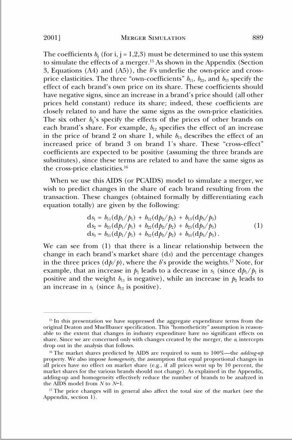
2001] Merger Simulation 889
The coefficients bij (for i, j = 1,2,3) must be determined to use this systemto simulate the effects of a merger.15 As shown in the Appendix (Section3, Equations (A4) and (A5)), the b’s underlie the own-price and cross-price elasticities. The three “own-coefficients” b11, b22, and b33 specify theeffect of each brand’s own price on its share. These coefficients shouldhave negative signs, since an increase in a brand’s price should (all otherprices held constant) reduce its share; indeed, these coefficients areclosely related to and have the same signs as the own-price elasticities.The six other bij’s specify the effects of the prices of other brands oneach brand’s share. For example, b12 specifies the effect of an increasein the price of brand 2 on share 1, while b13 describes the effect of anincreased price of brand 3 on brand 1’s share. These “cross-effect”coefficients are expected to be positive (assuming the three brands aresubstitutes), since these terms are related to and have the same signs asthe cross-price elasticities.16
When we use this AIDS (or PCAIDS) model to simulate a merger, wewish to predict changes in the share of each brand resulting from thetransaction. These changes (obtained formally by differentiating eachequation totally) are given by the following:
ds1 = b11(dp1/p1) + b12(dp2/p2) + b13(dp3/p3)ds2 = b21(dp1/p1) + b22(dp2/p2) + b23(dp3/p3) (1)ds3 = b31(dp1/p1) + b32(dp2/p2) + b33(dp3/p3) .
We can see from (1) that there is a linear relationship between thechange in each brand’s market share (ds) and the percentage changesin the three prices (dp/p), where the b’s provide the weights.17 Note, forexample, that an increase in p1 leads to a decrease in s1 (since dp1/p1 ispositive and the weight b11 is negative), while an increase in p2 leads toan increase in s1 (since b12 is positive).
15 In this presentation we have suppressed the aggregate expenditure terms from theoriginal Deaton and Muellbauer specification. This “homotheticity” assumption is reason-able to the extent that changes in industry expenditure have no significant effects onshare. Since we are concerned only with changes created by the merger, the ai interceptsdrop out in the analysis that follows.
16 The market shares predicted by AIDS are required to sum to 100%—the adding-upproperty. We also impose homogeneity, the assumption that equal proportional changes inall prices have no effect on market share (e.g., if all prices went up by 10 percent, themarket shares for the various brands should not change). As explained in the Appendix,adding-up and homogeneity effectively reduce the number of brands to be analyzed inthe AIDS model from N to N−1.
17 The price changes will in general also affect the total size of the market (see theAppendix, section 1).
World Composition Services ■ Sterling, VA ■ (703) 689-0900ABA: Antitrust LJ Vol. 69, No. 3, 2002 ■ ab3220ueps ■ 02-13-02 12:23:32
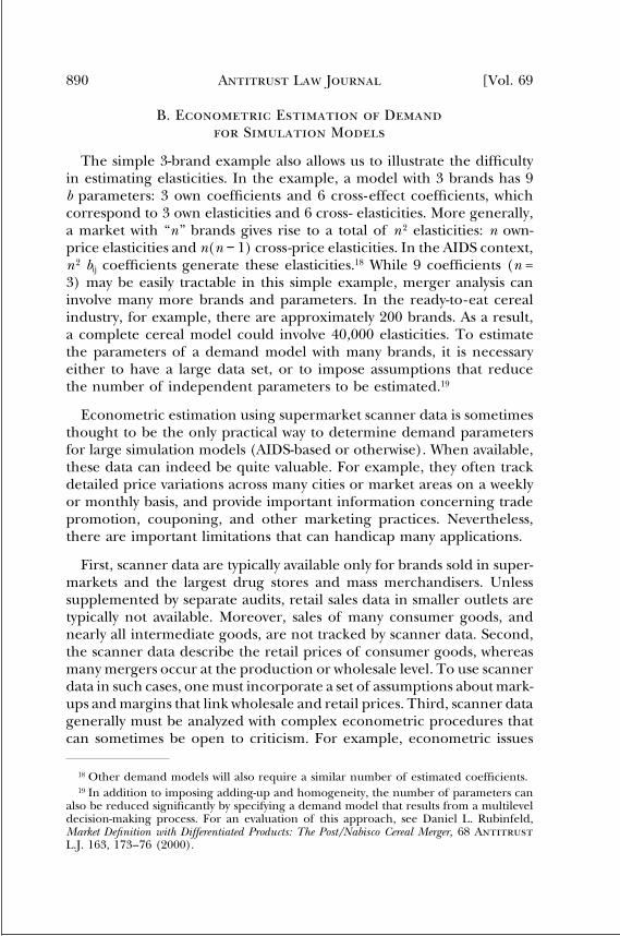
[Vol. 69Antitrust Law Journal890
B. Econometric Estimation of Demandfor Simulation Models
The simple 3-brand example also allows us to illustrate the difficultyin estimating elasticities. In the example, a model with 3 brands has 9b parameters: 3 own coefficients and 6 cross-effect coefficients, whichcorrespond to 3 own elasticities and 6 cross- elasticities. More generally,a market with “n” brands gives rise to a total of n 2 elasticities: n own-price elasticities and n(n − 1) cross-price elasticities. In the AIDS context,n 2 bij coefficients generate these elasticities.18 While 9 coefficients (n =3) may be easily tractable in this simple example, merger analysis caninvolve many more brands and parameters. In the ready-to-eat cerealindustry, for example, there are approximately 200 brands. As a result,a complete cereal model could involve 40,000 elasticities. To estimatethe parameters of a demand model with many brands, it is necessaryeither to have a large data set, or to impose assumptions that reducethe number of independent parameters to be estimated.19
Econometric estimation using supermarket scanner data is sometimesthought to be the only practical way to determine demand parametersfor large simulation models (AIDS-based or otherwise). When available,these data can indeed be quite valuable. For example, they often trackdetailed price variations across many cities or market areas on a weeklyor monthly basis, and provide important information concerning tradepromotion, couponing, and other marketing practices. Nevertheless,there are important limitations that can handicap many applications.
First, scanner data are typically available only for brands sold in super-markets and the largest drug stores and mass merchandisers. Unlesssupplemented by separate audits, retail sales data in smaller outlets aretypically not available. Moreover, sales of many consumer goods, andnearly all intermediate goods, are not tracked by scanner data. Second,the scanner data describe the retail prices of consumer goods, whereasmany mergers occur at the production or wholesale level. To use scannerdata in such cases, one must incorporate a set of assumptions about mark-ups and margins that link wholesale and retail prices. Third, scanner datagenerally must be analyzed with complex econometric procedures thatcan sometimes be open to criticism. For example, econometric issues
18 Other demand models will also require a similar number of estimated coefficients.19 In addition to imposing adding-up and homogeneity, the number of parameters can
also be reduced significantly by specifying a demand model that results from a multileveldecision-making process. For an evaluation of this approach, see Daniel L. Rubinfeld,Market Definition with Differentiated Products: The Post/Nabisco Cereal Merger, 68 AntitrustL.J. 163, 173–76 (2000).
World Composition Services ■ Sterling, VA ■ (703) 689-0900ABA: Antitrust LJ Vol. 69, No. 3, 2002 ■ ab3220ueps ■ 02-13-02 12:23:32

2001] Merger Simulation 891
involving model identification and estimation must be overcome beforedemand effects can be distinguished from supply effects. Finally, despiteone’s best efforts, econometric estimation may yield results at odds withcommon sense and intuition. With many parameters to be estimated, itis frequently the case that at least some of the empirically estimatedelasticities suffer from low levels of statistical significance, implausiblemagnitudes, and/or wrong algebraic signs.
C. PCAIDS: Proportionality-Calibrated AIDS
Calibrated-demand simulation models offer an alternative to modelsthat rely on econometric estimation of demand. Because they reducethe number of required demand parameters, these models are especiallyvaluable when there are data limitations or estimation problems, or whena rapid and less costly analysis is required.20 We offer Proportionality-Calibrated AIDS (PCAIDS) as a calibrated-demand model that providesanalytical flexibility while retaining many of the desirable propertiesof AIDS.
PCAIDS requires neither scanner data nor data on premerger prices.It requires information only on market shares, the industry price elastic-ity, and the price elasticity for one brand in the market. The logic ofPCAIDS is simple. The share lost as a result of a price increase is allocatedto the other firms in the relevant market in proportion to their respectiveshares. In effect, the market shares define probabilities of making incre-mental sales for each of the competitors.21
We believe that the proportionality assumption is practical and oftenreasonable when data are limited.22 With proportionality and PCAIDS,one can take a “quick look” at the likely price effects of a merger; theseresults are likely to be reliable when applied to markets with limitedproduct differentiation, or when the merger brands are not unusually
20 See Baker & Rubinfeld, supra note 1, for a survey of a variety of approaches to thecalibration of demand systems, including auction models and conjoint survey methods.
21 This approach has long been used in other settings involving economics and law whendata are limited. For example, in State Industries Inc. v. Mor-Flo Industries, Inc., 883 F.2d1573 (Fed. Cir. 1989), one of the leading decisions in the patent damages area, theassumption is that the patent holder suffers lost sales equal to its market share appliedto the infringer’s sales (the remaining infringing sales would have been made by the otherfirms in the market in proportion to their respective shares). For a recent analysis of thisdecision see Roy J. Epstein, State Industries and Economics: Rethinking Patent InfringementDamages, 9 Fed. Cir. B.J. 367 (2000).
22 Earlier discussions of proportionality in the context of merger analysis include RobertD. Willig, Merger Analysis, Industrial Organization Theory, and Merger Guidelines, in BrookingsPapers on Economic Activity: Microeconomics 299 (M. Baily & C. Winston eds., 1991);Shapiro, supra note 4.
World Composition Services ■ Sterling, VA ■ (703) 689-0900ABA: Antitrust LJ Vol. 69, No. 3, 2002 ■ ab3220ueps ■ 02-13-02 12:23:32

[Vol. 69Antitrust Law Journal892
close (or distant) in terms of their attributes and substitutability. In thissense, proportionality reflects the analytical framework in the MergerGuidelines, which suggest that market share sometimes may be used tomeasure the relative appeal of the merging firms’ products as first andsecond choices for consumers.23 Moreover, as we discuss below, PCAIDScan be extended to situations where extensive product differentiationmakes proportionality suspect. Indeed, PCAIDS can be used as an approx-imation of the AIDS model, with a structure that ensures proper signs andconsistent magnitudes for the elasticities.24 Another potential advantagecompared to other simulation methods is that PCAIDS can be imple-mented on a conventional spreadsheet without additional specializedsoftware. In summary, PCAIDS is a general method for calibrating AIDSdemand with minimal data, and for which proportionality is a usefulstarting point.
The simplifications that flow from the proportionality assumption ofPCAIDS can be illustrated in a simple example. The three equations inEquation (1) show that a change in the price of the first brand, p1, affectsthe market shares of all three brands. Recall that the own-effect of theprice of brand 1 on the share of brand 1 is b11. The cross-effects of p1
on the shares of brands 2 and 3 are given by b21 and b31. With proportional-ity, sales are diverted to brands 2 and 3 in proportion to the marketshares of the two brands. For example, if brand 2 has a share of 40percent and brand 3 a share of 20 percent, an increase in the price ofbrand 1 will increase the share of brand 2 by twice as much as it increasesthe share of brand 3. Formally, the proportionality assumption impliesthat the cross-effects associated with p1 can be expressed in terms of b11
and the observed shares; b21 is equal to −s2/(s2+s3)b11 and b31 equals−s3/(s2+s3)b11.25 The same relationships between own and cross effectshold for other prices; for example, b12 equals −s1/(s1+s3)b22.
The proportionality assumption reduces the number of unknown b’sin (1) from 9 to 3. We only need to know the 3 own-effect coefficients(and market shares) to calculate the remaining 6 cross-effect coefficients.More generally, the proportionality assumption posits a direct relation-
23 See Horizontal Merger Guidelines ¶ 2.211.24 Our discussion of PCAIDS focuses on implementation with aggregate market share
information. However, the method is also applicable as a set of restrictions that could beimposed when estimating standard AIDS with scanner data. We show in the Appendix thatPCAIDS and its extensions to non-proportionality satisfy Slutsky symmetry, an importanttheoretical property for demand systems.
25 The minus sign is necessary because b11 is negative (it is associated with the own-effect). It is easy to verify that the sum of the cross-effects in this case equals –b11, whichconfirms that adding-up is satisfied.
World Composition Services ■ Sterling, VA ■ (703) 689-0900ABA: Antitrust LJ Vol. 69, No. 3, 2002 ■ ab3220ueps ■ 02-13-02 12:23:32

2001] Merger Simulation 893
ship between all cross-effects associated with a particular price changeand the corresponding own-effect.26 The implication is that the onlyunknowns in the model are the n own-effect coefficients. The assumptionthat the predicted market shares sum to 100 percent eliminates oneadditional unknown, so the number of unknown parameters is thenreduced from n 2 to n − 1, or from 40,000 to 199 in our cereal example.
In fact, the proportionality assumption reduces the informationrequirement of PCAIDS even further. It is not necessary to know all n(or even n − 1) own-price effects or elasticities. The PCAIDS modelcan be calibrated with only two independent pieces of information (inaddition to the shares): the elasticity of demand for a single brand andthe elasticity for the industry as a whole. For example, only the industryelasticity and the own-price elasticity for brand 1 are needed as inputsin the calculation of the own-effect coefficient for brand 1, b11:
27
b11 = s1(ε11 + 1 − s1(ε + 1)). (2)
In Equation (2), ε11 is the own-price elasticity for brand 1 and ε is theindustry elasticity. Then, as shown in Section 4.A. of the Appendix,proportionality implies that all remaining unknown own-effect coeffi-cients can be determined as simple multiples of b11, as Equation (3)illustrates:
bii =si
1 − s1
1 − si
s1b11 . (3)
We have already seen that once the bii own-effects have been calculated,the cross-price effects can then be calculated from the own-price effectsand market shares. This means that knowledge of the own-price elasticityof any one brand and the overall industry price elasticity is sufficient toobtain estimates of all relevant demand parameters of the PCAIDS modelfrom the market share data. This is true whether there are 3 or 200brands.
Elasticities can be calculated directly from the values for the b parame-ters, the market shares (si), and the industry elasticity (ε), as follows (seeAppendix equations (A4) and (A5) for details):
26 Note that elasticities derived using the assumption of proportionality may be sensitiveto the market definition. If additional brands are thought to be in the market, and aretherefore included in the model, the estimated price effects of the merger could change.
27 More generally, the own-effect coefficient for any one brand can be determined fromthe industry elasticity and the own-price elasticity for that brand; the result is proven inthe Appendix.
World Composition Services ■ Sterling, VA ■ (703) 689-0900ABA: Antitrust LJ Vol. 69, No. 3, 2002 ■ ab3220ueps ■ 02-13-02 12:23:32

[Vol. 69Antitrust Law Journal894
Own-price elasticity for the ith brand:
εii = −1 +bii
si+ si(ε + 1). (4)
Cross-price elasticity of the ith brand with respect to the price of thejth brand:
εij =bij
si+ sj(ε + 1) . (5)
Under the assumption that the magnitude of the industry elasticity ε issmaller in magnitude than any brand own-price elasticity, PCAIDS impliesthat the cross-elasticities will be positive. Moreover, it can be shown thatall pre-transaction cross-elasticities corresponding to a given price changeare equal, i.e., εij = εkj for all brands i, j, and k. This equality is a conse-quence of the assumption of proportionality.28
All the information required to calibrate PCAIDS should be available.Market shares typically are known with reasonable accuracy. It shouldbe feasible to infer the own-price elasticity for at least one brand soldby the merging parties from marketing studies in the party’s documents(including surveys and focus groups), from econometric analyses, orfrom accounting data.29 The industry elasticity typically is considerablysmaller than the price elasticity of any one brand, because brand substitu-tion is easier than industry substitution.30 Absent independent informa-tion about the magnitude of that elasticity, we suggest an industryelasticity of −1 as a good starting point for a preliminary merger simula-tion. If the market under study is a relevant antitrust market, the industryelasticity will be equal to or greater than 1 in magnitude. As a result,this assumption will be conservative in its tendency to overpredict theprice effects of mergers.31
28 The assumption of proportionality is equivalent to the assumption of “Irrelevance ofIndependent Alternatives” (IIA) that underlies the logit model. Unlike the logit model,however, the PCAIDS post-merger elasticities are not constrained by IIA.
29 For an extensive discussion of the range of empirical methods that can be used toobtain estimates of demand elasticities, see Baker & Rubinfeld, supra note 1, Section 3.
30 Suppose the prices of all cereals rose by 10%. Because many consumers, particularlychildren, are likely to continue eating the same quantities of cereal for breakfast (some,of course, will not and consumption of cereal for other purposes, such as snacks, mayfall), ready-to-eat demand is not likely to be highly price-sensitive. On the other hand, a10% increase for a single brand, such as corn flakes, with no change in competitors’prices, will be more price-sensitive, because it will likely result in substantial switching toother products within the cereal category.
31 This follows from the rule of thumb for pricing by a monopolist. See, e.g., Pindyck& Rubinfeld, supra note 8, ch. 11.
World Composition Services ■ Sterling, VA ■ (703) 689-0900ABA: Antitrust LJ Vol. 69, No. 3, 2002 ■ ab3220ueps ■ 02-13-02 12:23:32

2001] Merger Simulation 895
To illustrate PCAIDS, reconsider the demand system in (1). Assumethat the shares for the 3 brands (each sold by a different firm) are 20%,30%, and 50%, respectively. Now, assume that there is a proposed mergerbetween firms 1 and 2, the industry elasticity is −1, and the own-priceelasticity for the first brand is −3. The formulas for PCAIDS given aboveand in the Appendix allow calculation of all parameters of the demandsystem (1) and all elasticities as shown in Table 1 below.
Table 1PCAIDS Coefficients and Elasticities
PCAIDS Coefficient with Respect to: Elasticity with Respect to:
Brand p1 p2 p3 Brand p1 p2 p3
1 −0.400 0.150 0.250 1 −3.00 0.75 1.252 0.150 −0.525 0.375 2 0.50 −2.75 1.253 0.250 0.375 −0.625 3 0.50 0.75 −2.25
The calculated own-elasticities—the negative values on the diagonalof the right panel of the table—can be either larger or smaller than theelasticity for the brand used to calibrate the system.32 Reading down eachcolumn of elasticities, the cross-elasticities corresponding to a given priceare equal, as expected given proportionality. PCAIDS simulation withthese parameters predicts a unilateral post-merger price increase (absentefficiencies) of 13.8% for Brand 1 and 10.8% for Brand 2.
D. Deviations from Proportionality—PCAIDS with Nests
Proportionality will not always characterize the diversion of lost salesaccurately when products are highly differentiated.33 Fortunately, it isstraightforward to modify PCAIDS to allow a more general analysis.Products that are closer substitutes for each other than proportionalitysuggests may be placed together in “nests.” The approach is analogousto using nests in a logit context, but we believe it is easier and moreflexible to calibrate PCAIDS with a nest structure.
32 The PCAIDS coefficients satisfy adding-up and homogeneity and are symmetric, asrequired.
33 Cf. Horizontal Merger Guidelines ¶ 2.211: “The market shares of the merging firms’products may understate the competitive effect of concern, when, for example, the prod-ucts of the merging firms are relatively more similar in their various attributes to oneanother than to other products in the relevant market. On the other hand, the marketshares alone may overstate the competitive effects of concern when, for example, therelevant products are less similar in their attributes to one another than to other productsin the relevant market.”
World Composition Services ■ Sterling, VA ■ (703) 689-0900ABA: Antitrust LJ Vol. 69, No. 3, 2002 ■ ab3220ueps ■ 02-13-02 12:23:32

[Vol. 69Antitrust Law Journal896
To illustrate, return to the three-brand example discussed in the previ-ous section. In that example, brand 2’s market share of 30% and brand3’s share of 50% implied that 37.5% (30/80) of the share lost by brand1 when its price increased would be diverted to brand 2 and 62.5% (50/80) would be diverted to brand 3. This effect can be characterized usingan odds ratio. Here, the odds ratio between brand 2 and brand 3 is 0.6(0.375/0.625). That is, under proportionality, brand 2 is only 60% aslikely to be chosen by consumers leaving brand 1 as brand 3. Now supposeinstead that brand 2 is relatively “farther” from brand 1 in the sense thatthat fewer consumers would choose brand 2 in response to an increasein p1 than would be predicted by proportionality. For example, brand 2may only be “half as desirable” a substitute as brand 3 and the appropriateodds ratio is really only 0.3. It is straightforward to calculate in this casethat the share diversion to brand 2 becomes 23.1% and the diversion tobrand 3 increases to 76.9% (an odds ratio of 0.3 = 0.231/0.769). Asexpected, fewer consumers leaving brand 1 would choose brand 2.
We generalize PCAIDS to cover such situations by constructing sepa-rate “nests” of brands. Diversion among brands within each nest is charac-terized by proportionality. Share diverted to a brand in a different nestdeviates from proportionality in the following sense: the odds ratio isequal to the odds ratio under proportionality, multiplied by an appro-priate scaling factor ranging from 0 to 1. The result is that brands withina nest are closer substitutes than brands outside the nest. PCAIDS withnests allows a more flexible pattern of cross-elasticities, as the model isno longer fully constrained by the proportionality assumption.
Continuing with the example, we capture the effect of brand 2 beinga less-close substitute for brand 1 than indicated by market shares byplacing brand 2 in a separate nest with a scaling or odds ratio factor of0.5. We then use formulas in the Appendix to recalculate the b coeffi-cients and resulting elasticities with this nesting assumption.34 Table 2reports the calculated elasticities for both the nested model and theoriginal model.35
The nest parameter rescales the cross-elasticities in the right-handpanel; the cross-elasticities measuring the responses of brands 2 and 3to the price of brand 1, and those measuring the responses of brands1 and 2 to the price of brand 3 are no longer equal. (The cross-elasticities
34 It would be incorrect to scale the non-nested elasticities in the left-hand panel directly.Nests affect adding-up, homogeneity, and symmetry and the appropriate calculation takesaccount of these constraints to generate economically consistent elasticities.
35 The calculations continue to assume an own-price elasticity of −3 for Brand 1 and anindustry elasticity of −1.
World Composition Services ■ Sterling, VA ■ (703) 689-0900ABA: Antitrust LJ Vol. 69, No. 3, 2002 ■ ab3220ueps ■ 02-13-02 12:23:32
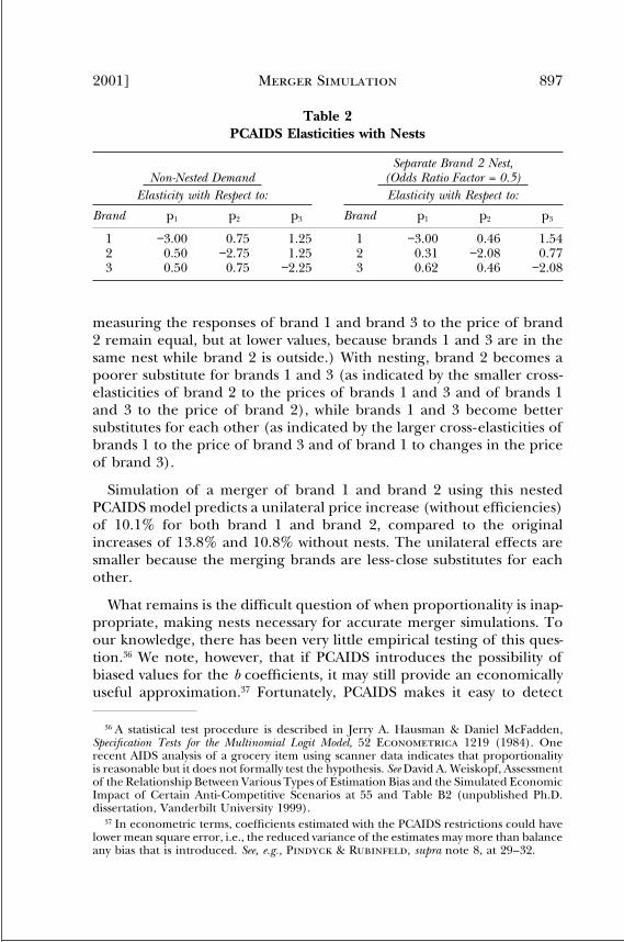
2001] Merger Simulation 897
Table 2PCAIDS Elasticities with Nests
Separate Brand 2 Nest,Non-Nested Demand (Odds Ratio Factor = 0.5)
Elasticity with Respect to: Elasticity with Respect to:
Brand p1 p2 p3 Brand p1 p2 p3
1 −3.00 0.75 1.25 1 −3.00 0.46 1.542 0.50 −2.75 1.25 2 0.31 −2.08 0.773 0.50 0.75 −2.25 3 0.62 0.46 −2.08
measuring the responses of brand 1 and brand 3 to the price of brand2 remain equal, but at lower values, because brands 1 and 3 are in thesame nest while brand 2 is outside.) With nesting, brand 2 becomes apoorer substitute for brands 1 and 3 (as indicated by the smaller cross-elasticities of brand 2 to the prices of brands 1 and 3 and of brands 1and 3 to the price of brand 2), while brands 1 and 3 become bettersubstitutes for each other (as indicated by the larger cross-elasticities ofbrands 1 to the price of brand 3 and of brand 1 to changes in the priceof brand 3).
Simulation of a merger of brand 1 and brand 2 using this nestedPCAIDS model predicts a unilateral price increase (without efficiencies)of 10.1% for both brand 1 and brand 2, compared to the originalincreases of 13.8% and 10.8% without nests. The unilateral effects aresmaller because the merging brands are less-close substitutes for eachother.
What remains is the difficult question of when proportionality is inap-propriate, making nests necessary for accurate merger simulations. Toour knowledge, there has been very little empirical testing of this ques-tion.36 We note, however, that if PCAIDS introduces the possibility ofbiased values for the b coefficients, it may still provide an economicallyuseful approximation.37 Fortunately, PCAIDS makes it easy to detect
36 A statistical test procedure is described in Jerry A. Hausman & Daniel McFadden,Specification Tests for the Multinomial Logit Model, 52 Econometrica 1219 (1984). Onerecent AIDS analysis of a grocery item using scanner data indicates that proportionalityis reasonable but it does not formally test the hypothesis. See David A. Weiskopf, Assessmentof the Relationship Between Various Types of Estimation Bias and the Simulated EconomicImpact of Certain Anti-Competitive Scenarios at 55 and Table B2 (unpublished Ph.D.dissertation, Vanderbilt University 1999).
37 In econometric terms, coefficients estimated with the PCAIDS restrictions could havelower mean square error, i.e., the reduced variance of the estimates may more than balanceany bias that is introduced. See, e.g., Pindyck & Rubinfeld, supra note 8, at 29–32.
World Composition Services ■ Sterling, VA ■ (703) 689-0900ABA: Antitrust LJ Vol. 69, No. 3, 2002 ■ ab3220ueps ■ 02-13-02 12:23:32

[Vol. 69Antitrust Law Journal898
whether nesting is likely have economically meaningful effects througha sensitivity analysis of the odds ratio factors. We suspect that mostsimulations will justify very few nests, because simulation results appearto be robust to modest departures from proportionality. We also believethat a coarse grid (e.g., 0.75, 0.50, and 0.25) covering a range of oddsratio factors is adequate to assess sensitivity.
E. PCAIDS and Other Calibrated-DemandSimulation Models
The PCAIDS model shares some characteristics with models based onlogit demand structures that have been used to simulate mergers. Bothassume proportionality (the logit model makes a comparable assump-tion of “independence of irrelevant alternatives”), yield positive cross-elasticities, and can be calibrated with only two parameters. We preferPCAIDS to logit, however, for several reasons. First, PCAIDS does notrequire premerger price data. There will doubtless be occasions whereprices are either not available for all firms in the market or are notmeasured accurately. Second, one can depart from proportionality inthe PCAIDS framework using nested demands. Logit models can begeneralized with nests as well, but we believe that logit is more difficultto calibrate econometrically and the additional nesting parameters areless intuitive.38 Third, we prefer PCAIDS because it has mathematical“curvature” that approximates that of the standard AIDS model.39 Wesuggest that the “curvature” of AIDS models is likely to fit data betterthan that of logit demand, although we recognize that this opinioninvites further empirical research.40 In essence, we view PCAIDS as adesirable mix of the best features of both logit (few parameters, correctsigns) and AIDS (ability to fit the data, curvature).41
38 For a discussion of estimation problems with nested logits, see Gregory J. Werden &Luke M. Froeb, The Effects of Mergers in Differentiated Products Industries: Logit Demand andMerger Policy, 10 J.L. Econ. & Org. 407, 420 (1994).
39 For an analysis of curvature of alternative demand models, see Crooke et al., supranote 12.
40 We are aware of very few studies that directly compare AIDS and logit using real-world data. A recent article that uses grocery scanner data on white pan bread salesindicates AIDS fit the data significantly better than logit. See Atanu Saha & Peter Simon,Predicting the Price Effect of Mergers with Polynomial Logit Demand, 7 Int’l J. Econ. Bus. 149,154 (2000).
41 The informative discussion at http://www.antitrust.org/mergers/economics/simulation.html concludes that “much progress has been made using the linear and nestedlogit demand specifications. . . . However, more progress can be made, by simulatingthe effects of mergers within the context of more flexible functional forms, like theAIDS model.”
World Composition Services ■ Sterling, VA ■ (703) 689-0900ABA: Antitrust LJ Vol. 69, No. 3, 2002 ■ ab3220ueps ■ 02-13-02 12:23:32
2001] Merger Simulation 899
Our approach is similar in spirit to one suggested by Carl Shapiro.42
Shapiro offers a rule-of-thumb formula for calculating the predictedprices of the post-merger firm, assuming that the merger involves twofirms and two symmetric merging brands. As inputs, he requires markups(or equivalently gross margins) and diversion ratios. Shapiro’s diversionratio-symmetry assumptions in his two-brand example are similar to ourproportionality assumption. However, his approach differs from ours ina number of ways. First, in much of the paper Shapiro assumes thatdemand elasticities are constant, an assumption that can create simula-tion difficulties because (a) such models sometime fail to converge; (b)the price increases resulting from a merger tend to be overstated; (c)non-merging firms do not raise prices in response to unilateral increasesby the merged entity. Second, his approach does not readily generalizeto multibrand firms. Finally, Shapiro does not discuss possible extensionswhen the proportionality assumption does not appear to be reasonable.
IV. USING PCAIDS
This section offers a number of examples of applications of PCAIDSthat are intended to make some of the principles discussed above moreconcrete. Our goal is to demonstrate that PCAIDS can provide reasonableestimates of the simulated effects of mergers at relatively low cost andwith some transparency. The examples demonstrate the calibration of thePCAIDS demand model using shares and elasticities, the incorporation ofefficiencies, sensitivity analyses using nests, and divestiture. The examplesutilize available data on toilet paper, baby food, and white pan bread.
A. The Kimberly-Clark/Scott Merger Revisited
We first use PCAIDS to re-examine the acquisition of Scott by Kimberly-Clark. A PCAIDS analysis of this 1992 merger may be compared to anearlier published simulation analysis by Hausman and Leonard thatused supermarket scanner data to estimate econometrically a standardAIDS model.43
There were eight toilet paper brands premerger with national sharesas shown in Table 3:
42 Shapiro, supra note 4; Carl Shapiro, Mergers with Differentiated Products, AddressBefore the ABA and IBA (Nov. 9, 1995), available at http://www.usdoj/atr/public/speeches/shapiro.spc.txt.
43 Jerry A. Hausman & Gregory K. Leonard, Economic Analysis of Differentiated ProductsMergers Using Real World Data, 5 Geo. Mason L. Rev. 321 (1997).
World Composition Services ■ Sterling, VA ■ (703) 689-0900ABA: Antitrust LJ Vol. 69, No. 3, 2002 ■ ab3220ueps ■ 02-13-02 12:23:32
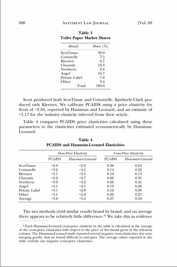
[Vol. 69Antitrust Law Journal900
Table 3Toilet Paper Market Shares
Brand Share (%)
ScotTissue 30.9Cottonelle 7.5Kleenex 6.7Charmin 12.4Northern 8.8Angel 16.7Private Label 7.6Other 9.4
Total 100.0
Scott produced both ScotTissue and Cottonelle. Kimberly-Clark pro-duced only Kleenex. We calibrate PCAIDS using a price elasticity forScott of −2.94, reported by Hausman and Leonard, and an estimate of−1.17 for the industry elasticity inferred from their article.
Table 4 compares PCAIDS price elasticities calculated using theseparameters to the elasticities estimated econometrically by Hausman-Leonard.
Table 4PCAIDS and Hausman-Leonard Elasticities
Own-Price Elasticity Cross-Price Elasticity
PCAIDS Hausman-Leonard PCAIDS Hausman-Leonard
ScotTissue −2.9 −2.9 0.36 0.24Cottonelle −3.2 −4.5 0.14 0.22Kleenex −3.1 −3.4 0.16 0.13Charmin −2.6 −2.7 0.66 0.35Northern −3.0 −4.2 0.26 0.41Angel −3.1 −4.1 0.19 0.26Private Label −3.1 −2.0 0.16 0.09Other −3.1 −2.0 0.20 0.27Average −3.0 −3.2 0.27 0.24
The two methods yield similar results brand by brand, and on averagethere appears to be relatively little difference.44 We take this as evidence
44 Each Hausman-Leonard cross-price elasticity in the table is calculated as the averageof the cross-price elasticities with respect to the price of the brand given in the left-mostcolumn. The Hausman-Leonard study reported several negative cross elasticities (for non-merging goods) that we found difficult to interpret. The average values reported in thetable exclude any negative cross-price elasticities.
World Composition Services ■ Sterling, VA ■ (703) 689-0900ABA: Antitrust LJ Vol. 69, No. 3, 2002 ■ ab3220ueps ■ 02-13-02 12:23:32
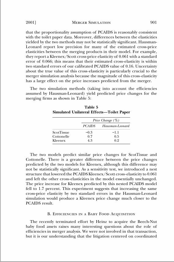
2001] Merger Simulation 901
that the proportionality assumption of PCAIDS is reasonably consistentwith the toilet paper data. Moreover, differences between the elasticitiesyielded by the two methods may not be statistically significant. Hausman-Leonard report low precision for many of the estimated cross-priceelasticities between the merging products in their model. For example,they report a Kleenex/Scott cross-price elasticity of 0.061 with a standarderror of 0.066; this means that their estimated cross-elasticity is withintwo standard errors of our calibrated PCAIDS value of 0.16. Uncertaintyabout the true value of this cross-elasticity is particularly crucial to themerger simulation analysis because the magnitude of this cross-elasticityhas a large effect on the price increases predicted from the merger.
The two simulation methods (taking into account the efficienciesassumed by Hausman-Leonard) yield predicted price changes for themerging firms as shown in Table 5:
Table 5Simulated Unilateral Effects—Toilet Paper
Price Change (%)
PCAIDS Hausman-Leonard
ScotTissue −0.3 −1.1Cottonelle 0.7 0.5Kleenex 4.3 0.2
The two models predict similar price changes for ScotTissue andCottonelle. There is a greater difference between the price changespredicted by the two models for Kleenex, although this difference maynot be statistically significant. As a sensitivity test, we introduced a neststructure that lowered the PCAIDS Kleenex/Scott cross-elasticity to 0.061and left the other cross-elasticities in the model essentially unchanged.The price increase for Kleenex predicted by this nested PCAIDS modelfell to 1.7 percent. This experiment suggests that increasing the samecross-price elasticity by two standard errors in the Hausman-Leonardsimulation would produce a Kleenex price change much closer to thePCAIDS result.
B. Efficiencies in a Baby Food Acquisition
The recently terminated effort by Heinz to acquire the Beech-Nutbaby food assets raises many interesting questions about the role ofefficiencies in merger analysis. We were not involved in that transaction,but it is our understanding that the litigation centered on coordinated
World Composition Services ■ Sterling, VA ■ (703) 689-0900ABA: Antitrust LJ Vol. 69, No. 3, 2002 ■ ab3220ueps ■ 02-13-02 12:23:32
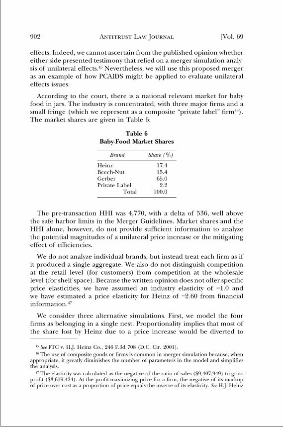
[Vol. 69Antitrust Law Journal902
effects. Indeed, we cannot ascertain from the published opinion whethereither side presented testimony that relied on a merger simulation analy-sis of unilateral effects.45 Nevertheless, we will use this proposed mergeras an example of how PCAIDS might be applied to evaluate unilateraleffects issues.
According to the court, there is a national relevant market for babyfood in jars. The industry is concentrated, with three major firms and asmall fringe (which we represent as a composite “private label” firm46).The market shares are given in Table 6:
Table 6Baby-Food Market Shares
Brand Share (%)
Heinz 17.4Beech-Nut 15.4Gerber 65.0Private Label 2.2
Total 100.0
The pre-transaction HHI was 4,770, with a delta of 536, well abovethe safe harbor limits in the Merger Guidelines. Market shares and theHHI alone, however, do not provide sufficient information to analyzethe potential magnitudes of a unilateral price increase or the mitigatingeffect of efficiencies.
We do not analyze individual brands, but instead treat each firm as ifit produced a single aggregate. We also do not distinguish competitionat the retail level (for customers) from competition at the wholesalelevel (for shelf space). Because the written opinion does not offer specificprice elasticities, we have assumed an industry elasticity of −1.0 andwe have estimated a price elasticity for Heinz of −2.60 from financialinformation.47
We consider three alternative simulations. First, we model the fourfirms as belonging in a single nest. Proportionality implies that most ofthe share lost by Heinz due to a price increase would be diverted to
45 See FTC v. H.J. Heinz Co., 246 F.3d 708 (D.C. Cir. 2001).46 The use of composite goods or firms is common in merger simulation because, when
appropriate, it greatly diminishes the number of parameters in the model and simplifiesthe analysis.
47 The elasticity was calculated as the negative of the ratio of sales ($9,407,949) to grossprofit ($3,619,424). At the profit-maximizing price for a firm, the negative of its markupof price over cost as a proportion of price equals the inverse of its elasticity. See H.J. Heinz
World Composition Services ■ Sterling, VA ■ (703) 689-0900ABA: Antitrust LJ Vol. 69, No. 3, 2002 ■ ab3220ueps ■ 02-13-02 12:23:32

2001] Merger Simulation 903
Gerber instead of Beech-Nut. The ratio of the Gerber to the Beech-Nutmarket share equals 65/15.4. This yields an odds ratio of 4.22, whichindicates that consumers leaving Heinz would be more than four timesas likely to shift to Gerber as to Beech-Nut. For the second simulation,we put Heinz and Beech-Nut in a separate nest from Gerber and privatelabel, with an odds ratio factor of 0.5. This nest structure represents thehypothesis that one group of consumers strongly prefers Gerber to Heinzand Beech-Nut. In this scenario the Gerber Beech-Nut odds ratio fallsby half to 2.11, indicating that Gerber becomes a poorer substitute (nowonly about twice as many consumers would choose Gerber). For thethird simulation, we put Heinz and private label in a separate nest fromGerber and Beech-Nut, also with an odds ratio factor of 0.5. This scenariotests the implication of treating Gerber and Beech-Nut as closer substi-tutes because they are both premium-priced brands. Since proportional-ity holds within a nest, the odds ratio would revert to 4.22 (the ratio oftheir market shares).
The simulated unilateral effects for each of these scenarios, in theabsence of any efficiencies, are given in Table 7:
Table 7Simulated Unilateral Effects—Baby Food
Simulated Price Change
Firm No Nests Heinz Beech-Nut Nest Beech-Nut Gerber Nest
Heinz 6.2% 12.3% 3.9%Beech-Nut 6.8% 13.3% 3.4%
These results illustrate the importance of the nesting assumption forthe magnitude of the price increases. Predicted price increases are largestwhen the merging firms are in the same nest (which implies consumersview them as closer substitutes for each other than market shares alonesuggest), and smallest when the merging firms are in separate nests(which implies consumers view then as less-close substitutes for eachother than market shares alone suggest).
PCAIDS can also be used to provide estimates of the efficiencies thatwould fully offset the predicted price effects. For the no-nest case, wecalculate that reductions in marginal costs of approximately 8% for bothHeinz and Beech-Nut would be required. If Heinz and Beech-Nut arecloser substitutes and in the same nest, reductions in marginal costs of
Company Form 10-K for fiscal year ended May 3, 2000, Consolidated Statements of Income,available at http://www.edgar-online.com.
World Composition Services ■ Sterling, VA ■ (703) 689-0900ABA: Antitrust LJ Vol. 69, No. 3, 2002 ■ ab3220ueps ■ 02-13-02 12:23:32

[Vol. 69Antitrust Law Journal904
approximately 16% for each firm are necessary to offset the predictedprice increase.
The Court notes that the merging parties claimed expected efficienciesof 22.3% for Beech-Nut.48 It is not clear to what extent the claimed cost-reductions for Beech-Nut would translate into merger-specific efficien-cies for the merged entity.49 However, our analysis in this hypotheticalsuggests that evidence on efficiencies would have been crucial to anyargument that unilateral effects of the merger on price were not likelyto be significant.
C. Merger with Divestiture
Some proposed transactions raise concerns about unilateral priceeffects that cannot be overcome by expected efficiencies or repositioning.Divestiture may be an option to “fix” such a deal, and simulation analysiscan help evaluate whether and which divestitures would eliminate com-petitive concerns. We illustrate an analysis of divestiture using data froma recent study of a merger between two large white pan bread bakeries.50
The pre-transaction market contained six firms with market shares asshown in Table 8:
Table 8Market Shares—White Pan Bread
Firm-Brand Share (%)
A-1 14.2A-2 8.1A-3 7.6B-1 8.8C-1 7.0D-1 7.6Grocery 31.5Other 15.2
Total 100.0
48 Heinz Co., 246 F.3d at 721.49 We understand (from personal communication) that Jonathan Baker testified (on
behalf of Beech-Nut and Heinz) to an expected 15% reduction in marginal cost for thegains passed through to the Beech-Nut brand. According to Baker, these gains wouldcome from a price reduction; the gains to Heinz buyers would come from getting a brandthat is 15% higher in quality (at the same price as their old brand, according to themerging parties).
50 See Saha & Simon, supra note 40.
World Composition Services ■ Sterling, VA ■ (703) 689-0900ABA: Antitrust LJ Vol. 69, No. 3, 2002 ■ ab3220ueps ■ 02-13-02 12:23:32

2001] Merger Simulation 905
Firms A and B are the merging parties. “Grocery” and “Other” arecomposites of smaller suppliers. The pre-transaction HHI was 2,317 witha change of 524, values that could trigger detailed agency review.
According to the study, the industry elasticity was −1.0. We set theelasticity for B-1 to the study’s estimate of −1.34 to complete the PCAIDScalibration of the demand model. Initially we assume proportionality.Table 9 shows the unilateral price increases for the merged firm predictedby PCAIDS in the absence of efficiencies.
Table 9Simulated Unilateral Effects—
White Pan Bread
Brand Price Increase
A-1 10.0A-2 10.0A-3 10.0B-1 28.7
The share-weighted average price increase for the brands in the mergeris 14.3%. Further analysis shows that even if the merger yielded efficien-cies that reduced the marginal costs of each brand by 10%, the PCAIDSsimulation would predict a price increase of approximately 18% for B-1.The share-weighted average price increase for the merged firm withthese efficiencies is 4.4%, which may still raise concerns. We also experi-mented with nests, since A-3 was a premium-priced brand and perhapswas less of a substitute for the lower-priced B-1. However, we did notfind that plausible nest structures significantly affected the results.51 With-out the prospect of timely entry or of efficiencies greater than 10%, thetransaction would certainly raise anticompetitive concerns.
Divestiture by Firm A of one or more of its three brands is one possiblestrategy to restructure the deal. The effect of divestiture on unilateralpricing behavior will depend both on what brand or brands are divestedand what firm acquires those brands. Simulation models can help analyzethe effects on prices of specific divestitures. We first simulated the mergerassuming a sale of A-3 to the smallest firm, C. For this merger anddivestiture, assuming no efficiencies, the predicted share-weighted aver-age price increase for the four brands originally sold by the merging
51 We even tried an extreme case of putting A-3 in a separate nest from all of the otherbrands in the market and setting the odds ratio factor to 0.01 to minimize the competitiveoverlap with B-1.
World Composition Services ■ Sterling, VA ■ (703) 689-0900ABA: Antitrust LJ Vol. 69, No. 3, 2002 ■ ab3220ueps ■ 02-13-02 12:23:32

[Vol. 69Antitrust Law Journal906
firms is only 2.8%. Even modest merger-related efficiencies would elimi-nate this average price increase. Alternatively, we simulated the mergerwith divestiture of A-3 to a hypothetical new entrant and found a share-weighted average price increase of only 1.8% before efficiencies.
The evaluation of these simulated post-divestiture price effects alsoraises the issue of appropriate measurement of prices. In our example,the range of price changes for the various brands is quite wide. Forexample, if A-3 is divested to firm C, its price is predicted to decrease by11.0%, while A-1 and A-2 have predicted price increases of 1.3% andB-1 has a predicted price increase of 18.6%. Divestiture reduces consider-ably the predicted price increases for brands the merged firm retainsand results in a predicted price decrease rather than increase for A-3.An important issue facing the merger authorities in this situation iswhether a transaction should be judged by its effect on average pricesin the relevant market, or by its separate effects on the prices for individ-ual brands.
V. ANALYZING PRODUCT REPOSITIONINGAND ENTRY WITH PCAIDS
The Horizontal Merger Guidelines acknowledge entry and productrepositioning as competitive responses to a merger with unilateral priceincreases.52 The Guidelines distinguish between “committed” entry,which requires significant sunk costs of entry and exit, and “uncommit-ted” entry, which does not.53 Uncommitted entrants are capable ofincreasing output sufficiently quickly (e.g., by redeploying existing assets)that they are able to constrain the market pre-transaction. For this reason,the Guidelines focus on committed entry as truly new competition thatmay be generated by unilateral price increases. For committed entry tobe an effective competitive check according to the Merger Guidelines,it must occur within two years (timeliness), must be profitable at pre-transaction prices (likelihood), and “must be responsive to the localizedsales opportunities that include the output reduction associated with thecompetitive effect of concern” (sufficiency).
Merger simulation (which could be based on PCAIDS or other demandmodels) provides a prediction of the unilateral price increases that wouldoccur absent entry or repositioning. Associated with any such priceincrease will be a reduction in output. The central question is whether
52 The Horizontal Merger Guidelines ¶ 2.12 n.23 indicates that the same analysis appliesto both cases.
53 See id. ¶¶ 1.0 & 3.0.
World Composition Services ■ Sterling, VA ■ (703) 689-0900ABA: Antitrust LJ Vol. 69, No. 3, 2002 ■ ab3220ueps ■ 02-13-02 12:23:32

2001] Merger Simulation 907
repositioning or entry can increase output sufficiently to defeat theprice increase.
A complete analysis of entry and repositioning raises difficult modelingissues that go beyond the scope of this article. It would require anassessment of sunk costs and minimum viable scale (the smallest scale atwhich its average cost is equal to the pre-transaction price) for committedentry, as well as a financial-accounting analysis to determine whetherpre-transaction prices are adequate for long-run profitability. Nonethe-less, we believe that PCAIDS can provide a useful framework in which toanalyze under the conditions under which committed and uncommittedresponses might be expected to constrain unilateral price increases.
We use the following procedure to identify the amount of entry thatshould be sufficient to eliminate unilateral price increases. For any brandsold by the merged firm, the post-merger revenue can be defined interms of the pre-merger revenue and the unilateral percent change inprice (δ*) and percent change in quantity (denoted α) for the brand.Since the shares and industry elasticity are known, and the merger simula-tion yields the unilateral price changes, it is possible to solve for thepercentage reduction in output α. Using the expression ppostqpost =(1+δ*)ppreqpre(1 − α), it can be shown that (see Section 4.D. of theAppendix for details)
α = 1 − spost
spre
(1 + (ε + 1)dP/P)(1 + δ*)
. (6)
The predicted output reduction therefore depends on two price ef-fects: the unilateral brand price increase and the average price change(dP/P) for the market as a whole.
The magnitude of the reduction in output in terms of the pre-transaction revenue market share for the brand is αs pre. If the entrant’ssales were a close substitute for the restricted output, then we couldexpect sales at this share level for the new brand to be sufficient toconstrain the merged firm at pre-transaction prices.54 The rationale isthat the sales opportunities of the entrant would effectively restore therestricted output to the market, implying a return to the pre-transactionprices.55 This analysis can be applied to solve for the value of α for each
54 Normally, we would expect the entrant to offer a close substitute, because entry isintended to take advantage of the sales opportunities resulting from unilateral priceincreases.
55 We implicitly assume that the combined sales of the entrant and the brand producedby the merged firm equal the pre-transaction level; that is, the entrant does not merely“cannibalize” sales from the incumbent.
World Composition Services ■ Sterling, VA ■ (703) 689-0900ABA: Antitrust LJ Vol. 69, No. 3, 2002 ■ ab3220ueps ■ 02-13-02 12:23:32

[Vol. 69Antitrust Law Journal908
brand sold by the merged firm for which unilateral price increases area concern. The total required entry would then be the sum of the sharesfrom the individual α factors.
The merger simulation may also indicate that other firms in the marketwould raise price and restrict output, generating additional sales opportu-nities. It may be appropriate to require additional entry to constrainthese price increases as well, in order to make sure that the entrant isnot diverted from pursuing the opportunities from the merged firm’soutput restrictions.
This analysis can, in principle, be applied to both uncommitted andcommitted repositioning. In the uncommitted case, sunk repositioningcosts are assumed to be zero. For committed repositioning, it is necessaryto carry out additional analyses to determine required sunk costs andminimum viable scale. As the Merger Guidelines point out, entry isunlikely if the minimum viable scale is larger than the sales opportunitiesavailable to entrants. In addition, the profits on the sales opportunitiesat pre-transaction prices must be sufficient to justify the sunk costs.
To illustrate some of the issues involved in an analysis of entry, weconsider a hypothetical transaction involving ready-to-eat (RTE) cere-als.56 RTE cereal products are highly differentiated along several dimen-sions (e.g., sweetness, texture, grains, vitamin and fiber content, colorand packaging). Because this example uses aggregated data and relieson other simplifying assumptions for purposes of illustration, we do notidentify individual companies or their product lines. In our examplethere are six firms: firms A, B, C, and D are “majors,” firm E is a privatelabel composite, and firm F is another composite firm that representsan aggregation of other, smaller brands. Firms C and D each sell twobrands. We use PCAIDS to analyze a hypothetical merger between firmsA and B.
We account for the fact that the characteristics of firms’ brands affectconsumers’ substitution patterns by placing the brands of the six firmsin two nests, based on whether each firm’s brands appeal primarily toadults or to children. (Each nest in the example could contain multiplebrands.) The premerger shares and nests are given in Table 10.57
Proportionality holds within each nest. We assume a scaling factor of50% for share diversion across nests. That is, the share diverted from a
56 We wish to thank Kraft Foods for providing us with the breakfast cereal data.57 We use the notions of Kids and Adult nests for illustrative purposes only. We believe,
nevertheless, that the relevant market for antitrust purposes is all ready-to-eat cereals. SeeNew York v. Kraft Gen. Foods, Inc., 926 F. Supp. 321, 356 (S.D.N.Y. 1995).
World Composition Services ■ Sterling, VA ■ (703) 689-0900ABA: Antitrust LJ Vol. 69, No. 3, 2002 ■ ab3220ueps ■ 02-13-02 12:23:32

2001] Merger Simulation 909
Table 10Pre-Merger Market Shares
Firm-Brand Share (%) Nest
A-1 13.0 KidsB-1 4.2 AdultC-1 26.5 KidsC-2 8.8 AdultD-1 21.8 KidsD-2 5.4 AdultPrivate Label 6.0 KidsOther 14.2 Kids
Total 100.0
Kids brand to an Adult brand (and vice versa) is only half as large aspredicted by their market shares. This structure introduces a simple, butflexible alternative to strict proportionality (with a factor of 100%).
To complete the data requirements for the simulation, we assume anindustry price elasticity of −1.0 and an own-price elasticity of −1.60 forA.58 We also assume that a merger between A and B will generate efficien-cies that lower incremental costs for each firm by 2%.
Taking into account the efficiencies (but not repositioning or entry),the PCAIDS simulation predicts that the merger will result in no changein A’s prices. However, the predicted price increase for B is 4.9% andits share falls to 4.1%. This post-merger price increase could raise compet-itive concerns, but it might also induce other firms to enter de novo orto redesign and reposition their products to compete more directlywith B.
We calculate the required entry to constrain B as follows. The valuefor α obtained from Equation (6) is 0.065. As a result, the value ofthe restricted output is 0.27 percentage points of market share (0.065multiplied by the pre-transaction share of 4.2%). If an entrant couldachieve this share with a new brand that is a close substitute for B thenthe unilateral price increase can be prevented.
The small amount of required entry in the example is not surprising,since B is a relatively small firm. (The amount of restricted output mustbe less than the size of B.) This highlights the potential importance ofthe analysis of minimum viable scale because entry on such a limited
58 The own-price elasticity for the example is calculated as the ratio of gross profits tosales from aggregate financial statements for A. A more refined estimate would requireinformation on sales and costs by product line.
World Composition Services ■ Sterling, VA ■ (703) 689-0900ABA: Antitrust LJ Vol. 69, No. 3, 2002 ■ ab3220ueps ■ 02-13-02 12:23:32

[Vol. 69Antitrust Law Journal910
basis may not be economic. In the RTE cereal industry, one possibilityfor low-cost entry might be repositioning of existing brands (or capacity)from the Kids segment to the Adult segment.
Ultimately it is a matter of judgment as to whether an entrant wouldbe capable of achieving the requisite share to make raising pricesunprofitable for the merging firm. Additional analysis would also benecessary to determine whether the entrant would achieve minimumviable scale and be profitable at pre-merger prices. Nevertheless, we areoptimistic that the approaches just described can provide a feasible anduseful framework to evaluate the range of issues raised when entry andrepositioning are discussed.
VI. PCAIDS AND THE MERGER GUIDELINES SAFE HARBORS
In this section we briefly discuss some applications of our simulationanalysis to the evaluation of safe harbor rules for unilateral effects. Asafe harbor offers a boundary below which transactions are not likelyto be challenged, thereby reducing transactions costs and conservingenforcement resources. The Merger Guidelines suggest two alternativesafe harbors with respect to unilateral effects. The first applies when thecombined market share of the merging firms is less than 35%; the otheris available when the change in the HHI is less than 50 (with a pre-transaction HHI over 1,800) or less than 100 (with a pre-transactionHHI between 1,000 and 1,800).59
If taken literally, the 35% safe harbor would shelter transactions fromreview for unilateral effects when the merging firms have shares as largeas 17.5% each, magnitudes that might not be uncommon. To evaluatethis safe harbor, we used PCAIDS (and reasonable elasticity assumptions)to investigate potential unilateral effects when the merging firms havea combined share of 35%.60 The results indicated price increases of 6%or more for at least one of the merging firms, irrespective of firm size.The simulations suggest that a 35% safe harbor runs too great a risk ofsheltering anticompetitive transactions.
Moreover, we note that the 35% standard, if enforced, would makethe HHI safe harbor virtually irrelevant for analyzing unilateral effects.
59 The Horizontal Merger Guidelines ¶¶ 2.211 and 2.22 leave open the possibility offinding significant unilateral effects when the merging firms have combined market sharesof less than 35%, indicating that this criterion is not equal in importance to the HHI safeharbor. For simplicity, however, we will refer to the 35% standard as a safe harbor andinvestigate its properties.
60 The simulations used an industry elasticity of −1, a brand elasticity of −3 for the firstmerger partner, and a third firm with a 65% share. There were no efficiencies or nests.
World Composition Services ■ Sterling, VA ■ (703) 689-0900ABA: Antitrust LJ Vol. 69, No. 3, 2002 ■ ab3220ueps ■ 02-13-02 12:23:32

2001] Merger Simulation 911
The only mergers not already protected by the 35% rule that would besheltered by the change in the HHI would be of minimal interest. Indeed,in these circumstances the smaller merging firm could have at most a1.5% share (pre-transaction HHI between 1,000 and 1,800) or a 0.7%share (pre-transaction HHI over 1,800). These constraints are inherentin the mathematics associated with the existing safe harbors (see Section5 of the Appendix for details), and are not dependent on our mergersimulation analysis.
We have separate concerns about the HHI safe harbor in cases involv-ing unilateral effects. The HHI safe harbor by itself shelters relativelyfew mergers because it is only satisfied when the smaller merging firmhas at most a 7% share (pre-transaction HHI between 1,000 and 1,800)or a 5% share (pre-transaction HHI over 1,800). Again, as shown in theAppendix, these limits follow directly from the definition of the safeharbor in the Merger Guidelines. By “protecting” only mergers involvingrelatively low market shares, the HHI safe harbors pose a low risk ofunilateral effects. This was confirmed by PCAIDS simulations that yieldedmaximum price increases under 5%.61
At the same time, it is natural to ask whether there is a basis for analternative safe harbor (perhaps tied to the HHI or the sum of marketshares) that could expedite a greater number of merger reviews whileproviding similar protection against anticompetitive transactions.62 Forexample, our preliminary investigation suggests that a 25% safe harborwould typically generate unilateral effects below 5%, using similarassumptions as before. Moreover, the weighted average price increasefor the merged firm will be even smaller when the merger partners aredifferent sizes. We realize, of course, that the choice of an alternativesafe harbor is a complex question that will involve substantial furtherstudy. However, the benefits in the form of reduced enforcement andtransaction costs could make this a worthwhile effort.
VII. CONCLUSION
Merger simulation can be used to evaluate many transactions that raisecompetitive concerns. It adds to the information provided by methodsthat rely on econometrically estimated demand systems, surveys of con-
61 The HHI simulations used an industry elasticity of −1, a brand elasticity of −3 for thefirst merger partner, and merging parties ranging from equal 5% shares to 24% and 1%shares, and a third firm with the residual share.
62 Other researchers who advocate simulation have found little support for the 35% ruleand have concluded that the existing HHI criterion “makes sense only if one believeseither that mergers are likely to generate no efficiencies or that only consumer welfareshould be considered in merger cases.” See Gregory J. Werden & Luke M. Froeb, Simulation
World Composition Services ■ Sterling, VA ■ (703) 689-0900ABA: Antitrust LJ Vol. 69, No. 3, 2002 ■ ab3220ueps ■ 02-13-02 12:23:32

[Vol. 69Antitrust Law Journal912
sumer preferences, and the analytical strategies described in the Horizon-tal Merger Guidelines. The PCAIDS simulation approach presented inthis article represents a simplification over existing techniques that webelieve offers advantages in many applications. It requires only aggregatemarket shares, the industry price elasticity, and the own-price elasticityfor a single brand in the relevant market. We have also shown that thisapproach can be easily extended to accommodate additional informationon substitution and diversion patterns by constructing product nests. Itallows a range of sophisticated analyses at relatively low cost. We haveprovided examples that evaluate efficiencies, nesting, brand divestiture,and entry/repositioning.
Our work is also relevant to recent criticisms of the use of marketshares, especially in the form of HHIs, for merger analysis. PCAIDSshows that market shares can be highly informative when combined withwell-grounded economic principles. In our view, the PCAIDS modeljustifies renewed reliance on market shares as a pragmatic benchmarkto assess competition. We note that the Merger Guidelines themselvesspell out the option of using market shares in an analysis of unilateraleffects when market shares are reliable indicators of the closeness ofsubstitutes and demand (which are essentially the conditions underwhich the proportionality assumption is appropriate).
Merger simulation is evolving and its techniques are improving. Weexpect that PCAIDS can help establish simulation as a standard tool toanalyze potential unilateral effects. We hope that the methods introducedin this article will provide a basis to evaluate options and possibilitiesthat might otherwise be quite difficult to subject to quantitative analysis.
as an Alternative to Structural Merger Policy in Differentiated Products Industries, in The Econom-ics of the Antitrust Process 77 (Malcolm B. Coate & Andrew N. Kleit eds., 1996).
World Composition Services ■ Sterling, VA ■ (703) 689-0900ABA: Antitrust LJ Vol. 69, No. 3, 2002 ■ ab3220ueps ■ 02-13-02 12:23:32

APPENDIX
Merger simulation builds on a demand-supply model that specifies aset of equations that relate three types of information for the brands inthe relevant market: (i) own and cross-price elasticities, (ii) marketshares, and (iii) gross profit margins. The demand model implies a“first-order condition” (FOC) for each brand, which specifies necessarymathematical relationships among these variables under the assumptionthat the firms in the market are maximizing profits without engaging inovert collusion. Each FOC involves the elasticities, shares, and marginsboth for that brand and for all of the other brands in the relevant marketowned by the same firm. In this way the FOCs take into account possibletrade-offs in pricing that are the primary source of unilateral effects.
1. Notation and AssumptionsA. There are n firms in the relevant market, each producing ni brands.
There are N brands in total.B. The jth brand has the following characteristics:
1. Average price pj
2. Quantity qj
3. Share sj of revenues in the relevant market4. Own-price elasticity εjj and cross-price elasticities εjk
5. Incremental cost cj and profit margin µj = (pj − cj)/pj.C. The average industry price is P, calculated as lnP = ∑silnpi, for i =
1 to N. Also, ∆P/P = ∑si(∆pi/pi).D. The n firms face an aggregate industry demand curve with a (pre-
merger) price elasticity of ε. An estimate of the percentage changein industry revenue due to industry-wide price changes is ∆(∑piqi)/∑piqi = ∆P/P(ε+1).
E. There is at least one known own-price elasticity εjj. Each known own-price elasticity is larger in magnitude than the industry elasticity ε,abs(εjj) > abs(ε), where abs(.) is the absolute value function.
F. Define the brand-specific vectors s = (s1, s2, . . ., sN)′ for marketshares, p = (p1, p2, . . ., pN)′ for prices, c = (c1, c2, . . ., cN)′ forincremental costs, and µ = (µ1, µ2, . . ., µN)′ for margins.
G. Define the brand-specific vector δ = (δ1, δ2, . . ., δN)′ of exponentialrates of price changes due to the transaction. Each δj = ln(pj
post)− ln(pj
pre). Define the brand-specific vector γ = (γ1, γ2, . . ., γN)′ of
913
World Composition Services ■ Sterling, VA ■ (703) 689-0900ABA: Antitrust LJ Vol. 69, No. 3, 2002 ■ ab3220ueps ■ 02-13-02 12:23:32
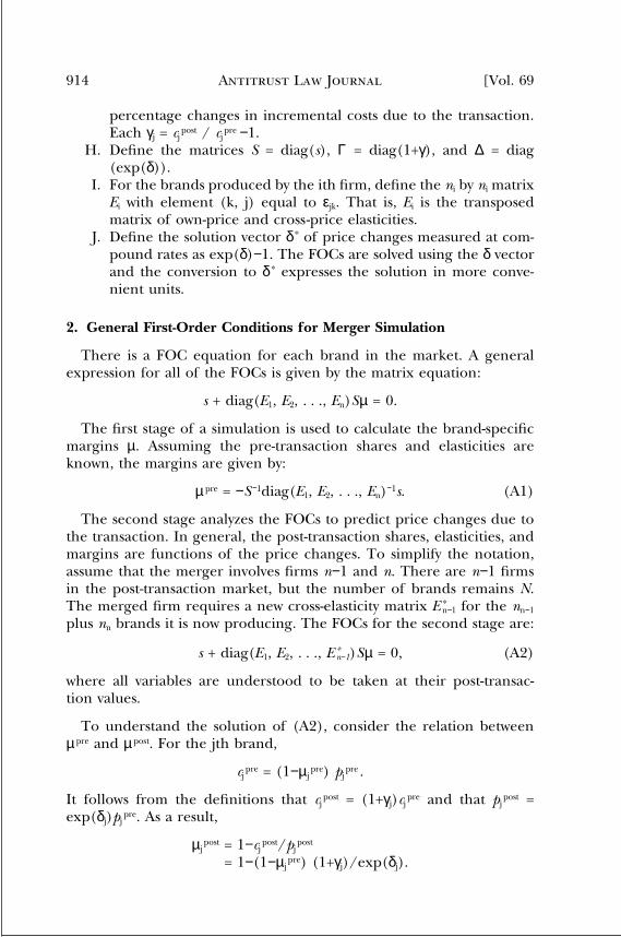
[Vol. 69Antitrust Law Journal914
percentage changes in incremental costs due to the transaction.Each γj = cj
post / cjpre −1.
H. Define the matrices S = diag(s), Γ = diag(1+γ), and ∆ = diag(exp(δ)).
I. For the brands produced by the ith firm, define the ni by ni matrixEi with element (k, j) equal to εjk. That is, Ei is the transposedmatrix of own-price and cross-price elasticities.
J. Define the solution vector δ* of price changes measured at com-pound rates as exp(δ)−1. The FOCs are solved using the δ vectorand the conversion to δ* expresses the solution in more conve-nient units.
2. General First-Order Conditions for Merger Simulation
There is a FOC equation for each brand in the market. A generalexpression for all of the FOCs is given by the matrix equation:
s + diag(E1, E2, . . ., En)Sµ = 0.
The first stage of a simulation is used to calculate the brand-specificmargins µ. Assuming the pre-transaction shares and elasticities areknown, the margins are given by:
µ pre = −S −1diag(E1, E2, . . ., En)−1s. (A1)
The second stage analyzes the FOCs to predict price changes due tothe transaction. In general, the post-transaction shares, elasticities, andmargins are functions of the price changes. To simplify the notation,assume that the merger involves firms n−1 and n. There are n−1 firmsin the post-transaction market, but the number of brands remains N.The merged firm requires a new cross-elasticity matrix E *
n−1 for the nn−1
plus nn brands it is now producing. The FOCs for the second stage are:
s + diag(E1, E2, . . ., E *n−1)Sµ = 0, (A2)
where all variables are understood to be taken at their post-transac-tion values.
To understand the solution of (A2), consider the relation betweenµpre and µpost. For the jth brand,
cjpre = (1−µj
pre) pjpre .
It follows from the definitions that cjpost = (1+γj)cj
pre and that pjpost =
exp(δj)pjpre. As a result,
µjpost = 1−cj
post/pjpost
= 1−(1−µjpre) (1+γj)/exp(δj).
World Composition Services ■ Sterling, VA ■ (703) 689-0900ABA: Antitrust LJ Vol. 69, No. 3, 2002 ■ ab3220ueps ■ 02-13-02 12:23:32
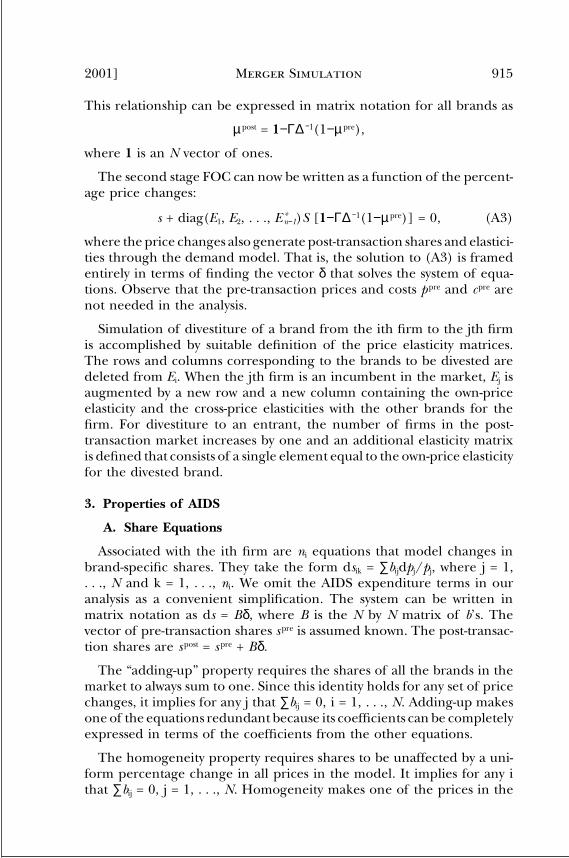
2001] Merger Simulation 915
This relationship can be expressed in matrix notation for all brands as
µpost = 1−Γ∆ −1(1−µpre),
where 1 is an N vector of ones.
The second stage FOC can now be written as a function of the percent-age price changes:
s + diag(E1, E2, . . ., E *n−1)S [1−Γ∆ −1(1−µpre)] = 0, (A3)
where the price changes also generate post-transaction shares and elastici-ties through the demand model. That is, the solution to (A3) is framedentirely in terms of finding the vector δ that solves the system of equa-tions. Observe that the pre-transaction prices and costs ppre and cpre arenot needed in the analysis.
Simulation of divestiture of a brand from the ith firm to the jth firmis accomplished by suitable definition of the price elasticity matrices.The rows and columns corresponding to the brands to be divested aredeleted from Ei. When the jth firm is an incumbent in the market, Ej isaugmented by a new row and a new column containing the own-priceelasticity and the cross-price elasticities with the other brands for thefirm. For divestiture to an entrant, the number of firms in the post-transaction market increases by one and an additional elasticity matrixis defined that consists of a single element equal to the own-price elasticityfor the divested brand.
3. Properties of AIDS
A. Share Equations
Associated with the ith firm are ni equations that model changes inbrand-specific shares. They take the form dsik = ∑bijdpj/pj, where j = 1,. . ., N and k = 1, . . ., ni. We omit the AIDS expenditure terms in ouranalysis as a convenient simplification. The system can be written inmatrix notation as ds = Bδ, where B is the N by N matrix of b’s. Thevector of pre-transaction shares spre is assumed known. The post-transac-tion shares are spost = s pre + Bδ.
The “adding-up” property requires the shares of all the brands in themarket to always sum to one. Since this identity holds for any set of pricechanges, it implies for any j that ∑bij = 0, i = 1, . . ., N. Adding-up makesone of the equations redundant because its coefficients can be completelyexpressed in terms of the coefficients from the other equations.
The homogeneity property requires shares to be unaffected by a uni-form percentage change in all prices in the model. It implies for any ithat ∑bij = 0, j = 1, . . ., N. Homogeneity makes one of the prices in the
World Composition Services ■ Sterling, VA ■ (703) 689-0900ABA: Antitrust LJ Vol. 69, No. 3, 2002 ■ ab3220ueps ■ 02-13-02 12:23:32

[Vol. 69Antitrust Law Journal916
model redundant because its coefficients can be completely expressedin terms of the coefficients for the other prices in the same equation.
B. AIDS Own-Price Elasticities
εii =∂qi
∂pi
pi
qi= (−qi
pi+
bii
pi
PQpi
+si
pi
∂PQ∂pi
) pi
qi
(A4)
= −1 +bii
si+
pi
PQ∂PQ∂pi
= −1 +bii
si+
pi
∂pi
∂PP
(ε + 1)
= −1 +bii
si+ s i (ε + 1).
C. AIDS Cross-Price Elasticities
εij =∂qi
∂pj
pj
qi= (−bij
pj+
PQpi
+si
pi
∂PQ∂pj
) pj
qi
=bij
si+ sj(ε + 1). (A5)
4. Properties of PCAIDS
A. PCAIDS Calibration of the Demand System
We now show that PCAIDS can be fully calibrated regardless of thenumber of brands in the market, using only information on the own-price elasticity of demand for a single brand, the industry price elasticityof demand, and the market share data. The same result holds for theextension of the method using nests.
Each element of B can be written as bik = θikbkk, where the θ’s are knownbut the diagonal elements bkk are unknown. The relative share diversionbetween brand i and brand j for a price change in brand k is given bythe odds ratio θik/θjk. For example, under strict proportionality θik =−si/(1−sk) and the odds ratio equals si/sj. Impose adding-up and homogeneity.The constraints imply a system of N−1 independent equations in the Nunknown own-coefficients. Without loss of generality, assume that ε11 isknown. We normalize with respect to the first brand and define a vectorβ with N−1 elements equal to bjj/b11 = βj, j > 1. The equation system isthen non-singular and can be written in matrix form as
�θ12 θ13 ... θ1N
1 θ23 ... θ2N
�
θN−1,2 ... 1 θN−1,N
� � β2
�
βN� = �
−1
−θ21
�
−θN−1,1
� (A6)
World Composition Services ■ Sterling, VA ■ (703) 689-0900ABA: Antitrust LJ Vol. 69, No. 3, 2002 ■ ab3220ueps ■ 02-13-02 12:23:32

2001] Merger Simulation 917
(A6) can be inverted to solve for the β vector, which will be a functionof the market shares. It can be shown that each βi equals [(1−si)/(1−s1)](si/s1).
Since ε11 and ε are known, we can invert the formula for own-priceelasticity to find b11 = s1(ε11 + 1 − s1(ε + 1)). The PCAIDS system cantherefore be calibrated completely using market shares and the two elas-ticities.
We now prove that each PCAIDS own-price elasticity is larger in magni-tude than the industry elasticity. By assumption, abs(ε11) > abs(ε). Assumethat abs(εii) < abs(ε) for some i > 1. Substituting bii=[(1−si)/(1−sj)](si/sj)b11 in the expression for the own price elasticity for εii yields the contra-diction that abs(ε11) < abs(ε).
Finally, we prove that all PCAIDS cross-price elasticities are greaterthan zero. Suppose εik < 0 for some i, k. By substitution, this implies−bkk/(1−sk)+sk(ε+1)<0. Substitute for bkk in terms of εkk, and rearrangeyielding the implication ((εkk+1)−sk(ε+1))sk > (1−sk)sk(ε+1). However,since εkk < ε, this is a contradiction.
B. PCAIDS Nests
Assume that there are w nests, w ≤ N, with each brand assigned to anest. Given a price increase for brand k in nest f1, the diversion of shareto brand i in nest f2 deviates from proportionality by a multiplicativefactor ω(k, i) > 0. We assume that ω(k, i) = ω(i, k). Similarly, the diversionfrom brand k to brand j in nest f3 deviates from proportionality by ω(k,j). Proportionality is the special case where ω(k, i) = 1. It can be shownin this general setting that:
θik = −siω(k,i)
∑m ≠ k smω(k,m).
The odds ratio under nesting is θik/θjk = (si/sj)[ω(k,i)/ω(k,j)]. In thecase of proportionality for all nests, this reduces to the familiar si/sk.
C. Slutsky Symmetry of B with PCAIDS
We now show that the matrix B of PCAIDS coefficients is symmetricboth under strict proportionality and with nests as we have definedthem. The discussion in Section 4.A implies that, under adding up andhomogeneity, βj = θj1/θ1j. It follows that
βj =sj
s1
∑m≠jsmω(j,m)
∑m≠1smω(1,m)
and from before, bjj = βjb11.
World Composition Services ■ Sterling, VA ■ (703) 689-0900ABA: Antitrust LJ Vol. 69, No. 3, 2002 ■ ab3220ueps ■ 02-13-02 12:23:32

[Vol. 69Antitrust Law Journal918
By the definition of B and substitution for βi and βj,
bij =sisj
s1
ω(i,j)
∑N
k=2skω(k,1)
b11 .
for i≠j. Symmetry of B follows directly.
D. Required Market Share for Entry to Defeat Unilateral Effects
Let α represent the unilateral output reduction. For any brand pro-duced by the merged firm, post-transaction revenue ppostqpost is relatedto pre-transaction revenue p preq pre as follows:
p postq post = (1+δ*)p preq pre(1−α),
where δ* is the unilateral percentage price increase. Total post-transac-tion market revenue equals pre-transaction market revenue PQ multi-plied by 1+(ε+1)dP/P, where P is the average market price change (see1.D.). Dividing both sides of the equation by post-transaction marketrevenue yields
p postq post
PQ(1 + (ε + 1)dP/P)= (1 + δ*)
p preq pre
PQ(1 + (ε + 1)dP/P)(1 − α) .
Rewrite in terms of shares as
spost = (1 + δ*)s pre
(1 + (ε + 1)dP/P)(1 − α)
and solve for α as
α = 1 − s post
s pre
(1 + (ε + 1)dP/P)(1 + δ*)
.
5. Proof of Maximum Firm Sizes Under Merger Guidelines SafeHarbors
If the 35% safe-harbor rule were enforced, then the HHI safe harborwould have independent relevance only for transactions where one ofthe firms is very small. By the algebra of the HHI (see Merger Guidelinesat note 18), the safe harbor for merging firms 1 and 2 can be expressed as:
2s1s2 < δ,
where δ, the maximum safe harbor change in the HHI, is either 100(pre-HHI less than 1,800) or 50 (pre-HHI greater than 1,800). It followsthat s2 < δ/(2s1).
By assumption, s1 + s2 > 35%, so that s2 > 35% − s1. Putting these twoconditions together implies
World Composition Services ■ Sterling, VA ■ (703) 689-0900ABA: Antitrust LJ Vol. 69, No. 3, 2002 ■ ab3220ueps ■ 02-13-02 12:23:32
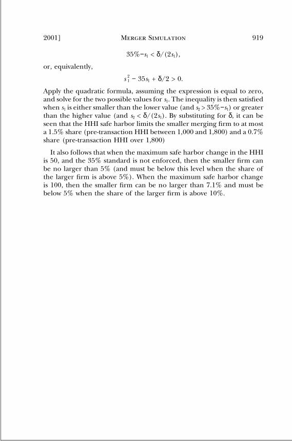
2001] Merger Simulation 919
35%−s1 < δ/(2s1),
or, equivalently,
s 21 − 35s1 + δ/2 > 0.
Apply the quadratic formula, assuming the expression is equal to zero,and solve for the two possible values for s1. The inequality is then satisfiedwhen s1 is either smaller than the lower value (and s2 > 35%−s1) or greaterthan the higher value (and s2 < δ/(2s1). By substituting for δ, it can beseen that the HHI safe harbor limits the smaller merging firm to at mosta 1.5% share (pre-transaction HHI between 1,000 and 1,800) and a 0.7%share (pre-transaction HHI over 1,800)
It also follows that when the maximum safe harbor change in the HHIis 50, and the 35% standard is not enforced, then the smaller firm canbe no larger than 5% (and must be below this level when the share ofthe larger firm is above 5%). When the maximum safe harbor changeis 100, then the smaller firm can be no larger than 7.1% and must bebelow 5% when the share of the larger firm is above 10%.
World Composition Services ■ Sterling, VA ■ (703) 689-0900ABA: Antitrust LJ Vol. 69, No. 3, 2002 ■ ab3220ueps ■ 02-13-02 12:23:32