technical memorandum permittable water use...
TRANSCRIPT

TECHNICAL MEMORANDUM
PERMITTABLE WATER USE ESTIMATESOF THE
FLORIDAN AQUIFER SYSTEMIN THE
UPPER EAST COAST PLANNING AREA
A Technical Support Study for theResource Control Department
Richard F. Bower
June 1988
Hydrogeology DivisionResource Planning Department
South Florida Water Management District

TECHNICAL MEMORANDUM
PERMITTABLE WATER USE ESTIMATESOF THE
FLORIDAN AQUIFER SYSTEMIN THE
UPPER EAST COAST PLANNING AREA
A Technical Support Study for theResource Control Department
Richard F. Bower
June 1988
Hydrogeology DivisionResource Planning Department
South Florida Water Management District
This publication was produced on recycled paper.

EXECUTIVE SUMMARY
The entire Upper East Coast Planning Area is a discharge area for the Floridan
Aquifer System. Throughout most of the area, the potentiometric surface of the
Floridan Aquifer System is not only above the water table, but also above land
surface by as much as 15 to 35 feet.
In order to protect legal uses of the Floridan Aquifer System from loss of free
flow from wells not equipped with pumps, the South Florida Water Management
District (SFWMD) has adopted a rule generally prohibiting installation of pumps on
Floridan Aquifer System wells in Martin and St. Lucie Counties for the purpose of
increasing natural flow rates.
In 1981, SFWMD's Resource Control Department staff evaluated irrigation
water use and surface water management systems for a proposed 11,833-acre citrus
grove located in northwestern St. Lucie County. It was determined that the
maximum withdrawal rate which could be made without the installation of pumps
on proposed wells is 14 MGD, which is equivalent to 1.5 inches per acre per month.
The criterion of a maximum month allocation of 1.5 inches per acre was extended to
include the entire western C-25 basin in SFWMD Permit Information Manual,Volume III, Management of Water Use, adopted June, 1985.
Application of the 1.5 inch per acre maximum month allocation criterion to all
of Martin & St.Lucie Counties has been suggested. However, some evaluation of the
reliability and reasonability of the use of the criterion on a regional basis is needed.
The means for making the evaluation is a numerical flow model developed for the
Floridan Aquifer System in the Upper East Coast Planning Area. The Floridan
Aquifer System is viewed conceptually as three layers; the Upper Floridan Aquifer,
the intra-aquifer confining bed, and the Lower Floridan Aquifer. The model
simulates conditions in the Upper Floridan Aquifer where most of the flow in the
aquifer system occurs, and where most of the wells in the study area are completed.

In the first part of the evaluation process, a withdrawal of 1.5 inches/acre is
made from all nodes with positive head relative to land surface; simulated drawdown
is well below land surface in all nodes, demonstrating that a maximum month
criterion of 1.5 inches/acre cannot be applied regionally without ultimately causing
free flow from Floridan wells to cease.
In the next part, the model was run iteratively to determine maximum
withdrawal which could be made from each node while still maintaining some
positive head. By attempting to maximize withdrawals throughout the aquifer,
rates as high as the proposed 1.5 inches/acre are obtained in few nodes.
It is concluded that the 1.5 inches/acre limitation is valid, but only
site-specifically; regional application generates drawdowns which cause free flow to
cease. It is recommended that interim water use management be accomplished by
using the existing two-dimensional model for cumulative impact evaluations of new
or increased allocations from the Floridan Aquifer System and that the model be
redeveloped using a fully three dimensional flow code for use in the ultimate
management strategy for the Floridan Aquifer.

TABLE OF CONTENTS
EXECUTIVE SUMMARY ............... .....................
LIST OF FIGURES ............. . ..... ........................... v
LIST OF TABLES .................. ................. ........ v
ACKNOWLEDGEMENTS .......................................... v
ABSTRACT ..................... ******* * * ......... .........
INTRODUCTION ................................................ 1
COMPUTER SIMULATION OF GROUND WATER FLOWIN THE UPPER FLORIDAN AQUIFER SYSTEM ..................... 4
EVALUATION OF ALLOCATION CRITERIA ......... 2................. 24
CONCLUSIONS AND RECOMMENDATIONS ........................ 32
APPENDIX A ........................................................ A-1
iii
LIST OF FIGURES
Figure Page
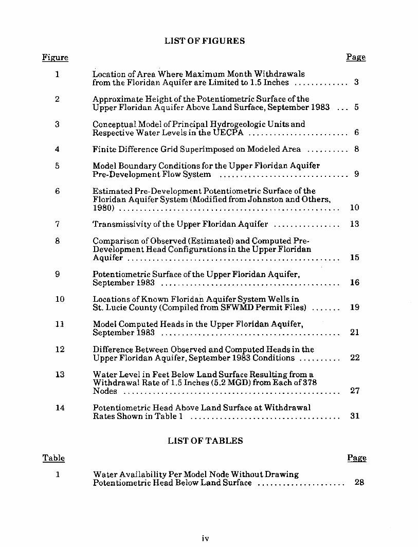
1 Location of Area Where Maximum Month Withdrawalsfrom the Floridan Aquifer are Limited to 1.5 Inches ............ 3
2 Approximate Height of the Potentiometric Surface of theUpper Floridan Aquifer Above Land Surface, September 1983 ... 5
3 Conceptual Model of Principal Hydrogeologic Units andRespective Water Levels in the UECPA ................................ 6
4 Finite Difference Grid Superimposed on Modeled Area .......... 8
5 Model Boundary Conditions for the Upper Floridan AquiferPre-Development Flow System ............................... 9
6 Estimated Pre-Development Potentiometric Surface of theFloridan Aquifer System (Modified from Johnston and Others,1980) ..................................................... 10
7 Transmissivity of the Upper Floridan Aquifer ................ 13
8 Comparison of Observed (Estimated) and Computed Pre-Development Head Configurations in the Upper FloridanAquifer ................................................... 15
9 Potentiometric Surface of the Upper Floridan Aquifer,September 1983 ........................................... 16
10 Locations of Known Floridan Aquifer System Wells inSt. Lucie County (Compiled from SFWMD Permit Files) ....... 19
11 Model Computed Heads in the Upper Floridan Aquifer,September 1983 ......................... ... ..... .......... 21
12 Difference Between Observed and Computed Heads in theUpper Floridan Aquifer, September 1983 Conditions .......... 22
13 Water Level in Feet Below Land Surface Resulting from aWithdrawal Rate of 1.5 Inches (5.2 MGD) from Each of 378Nodes .................................................... 27
14 Potentiometric Head Above Land Surface at WithdrawalRates Shown in Table .................................... 31
LIST OF TABLES
Table Page
1 Water Availability Per Model Node Without DrawingPotentiometric Head Below Land Surface .................... 28

ACKNOWLEDGEMENTS
The author thanks the following individuals for invaluable assistance in the
development of this report: Sharon Trost, who developed the prototype of the finite-
difference model used in this project, and who provided knowledge and insight based
upon her previous work with the Floridan Aquifer system in the Upper East Coast
Planning Area; Diane Bello, who prepared most of the illustrations in this report;
and Hedy Marshall, who prepared the text portion of the report in various drafts as
well as the final version.

ABSTRACT
The regional applicability of certain District rules governing withdrawals from
portions of the Floridan Aquifer System are evaluated using a finite-difference flow
model. The United States Geologic Survey two-dimensional flow code is used in a
quasi-three-dimensional configuration; upward leakance from the lower to the upper
Floridan Aquifer System is simulated by leakage and diffuse upward leakance from
the upper Floridan Aquifer System is simulated as negative recharge. Imposed
stress from agricultural withdrawals, the least reliably known parameter, is used to
obtain the final calibration. The regional applicability of a rule limiting Floridan
Aquifer withdrawals to 1.5 acre-inches per month is evaluated by applying that rate
to all model nodes corresponding to areas where free flow occurs; the drawdown
generated in this scenario causes all water levels in the Floridan Aquifer System to
fall below land surface, meaning that freeflow from wells would cease. The rule
forbidding installation of pumps on flowing wells, thereby limiting drawdown in the
Floridan Aquifer to land surface, is also evaluated. The model was run iteratively to
determine maximum withdrawal from each node while maintaining free flow;
generally, nodal withdrawal rates range between 0.1 and 1.0 inch. It is concluded
that the 1.5 acre-inch criterion has been validly applied site-specifically, but cannot
be applied regionally. The existing two-dimensional model can be used for interim
management of the Floridan Aquifer System; however, to more accurately reflect the
physical system, particularly when stressed, a fully three-dimensional model with a
finer grid is recommended.

INTRODUCTION
In order to protect legal uses of the water from Floridan Aquifer System from
loss of free flow from wells not equipped with pumps, the South Florida Water
Management District (SFWMD) has adopted the following rule:
3.2.2.4.9.2 Pumps on Floridan Wells in Martin and St. Lucie Counties -No pump shall be placed on a Floridan well in Martin or St. Lucie county exceptunder the following guidelines:
1) The pump was in place and operational on the well prior to March 2, 1974.
2) The pump which is proposed for installation, is a centrifugal pumpinstalled for the purpose of increasing pressure in attached piping (i.e.drip or jet irrigation systems) and not for the purpose of increasing flowover and above that flow which naturally emanates from the well...
Prior to the adoption of the rule in 1985, this policy was included as a limiting
condition on water use permits issued within the St. Lucie basin.
In 1981, the staff of the Resource Control Department met with the Orange
Avenue Growers Citrus Association regarding conceptualization of both irrigation
water use and surface water management systems for a 11,833-acre project located
in northwestern St. Lucie County. Because water use permits issued to the
Association for Floridan Aquifer withdrawals would be subject to the free-flow
limiting condition, the Resource Control Department staff decided that the
allocations authorized by those permits should reflect the estimated amount of water
available from the Floridan Aquifer System while maintaining positive
potentiometric pressure above land surface over the project site. An analytical
drawdown model emulating the Theis non-equilibrium flow equation was used to
estimate the amount of water available. The selected transmissivity value of
500,000 GPD/ft and storativity value of .0005 were estimated from SFWMD
Technical Publication 80-1. Representatives of the Orange Avenue Citrus Growers
Association informed staff that the longest period of sustained withdrawal from the
Floridan would be 90 days. Staff determined that, on the average, potentiometric

head in the Floridan Aquifer occurred at 15 feet above the land surface of the project
site. Utilizing these parameters, the Theis model was set up to simulate 60
withdrawal points located on half-mile centers throughout the project site, then run
at increasing withdrawal rates until a projected drawdown which was slightly less
than 15 feet was obtained (Appendix A). This condition was produced by a
withdrawal of 14 MGD, which is equivalent to 1.5 acre-inches per month applied to
10,640 proposed irrigated acres.
In February, 1984, Water Use Permit 56-00473-W was issued to Orange
Avenue Citrus Growers Association authorizing withdrawals from the Floridan
Aquifer not to exceed 381 MG/month (1.5 acre-inches X 9358 acres). The criterion of
a maximum month allocation of 1.5 acre-inches was extended to include the entire
western C-25 basin in SFWMD Permit Information Manual, Volume III,
Management of Water Use, adopted June, 1985, as follows:
3.2.2.4.9.1 Allocation of Floridan Aquifer Water in the EasternOkeechobee-Northwestern St. Lucie Basin - When the project site islocated within the Eastern Okeechobee-Northwestern St. Lucie basin,withdrawals from the Floridan Aquifer are limited to 1.5 inch for themaximum month, with the balance of the water needs being withdrawn fromother sources.
Application of the 1.5 acre-inch maximum month allocation criterion to all of
Martin & St.Lucie Counties has been suggested. However, some evaluation of the
reliability and reasonability of the use of the criterion on a regional basis is needed.
The means for making the evaluation is a numerical flow model developed as
part of an unpublished report of the hydrogeology of the Floridan Aquifer System in
the Upper East Coast Planning Area. Although the Floridan Aquifer System is
multi-layered within Martin & St.Lucie Counties, unavailability of the USGS
three-dimensional modular flow code (MODFLOW) at the time of model
development required use of the USGS two-dimensional flow code instead. A
quasi-three-dimensional approach is used, whereby leakance from the lower to the

SLEMNDS - W Oe lmoumAI
ILES USSa s - UA oUN1D
Figure 1. Location of Area Where Maximum Month Withdrawals from theFloridan Aquifer are Limited to 1.5 Inches
3

upper Floridan Aquifer System is simulated with the leakage option of the code, and
diffuse upward leakance out of the Upper Floridan Aquifer is simulated as negative
recharge.
COMPUTER SIMULATION OF GROUND WATER FLOW IN
THE UPPER FLORIDAN AQUIFER SYSTEM
Introduction
The pre-development steady-state flow system is simulated in order to quantify
the volume of water flowing through the aquifer prior to development and to verify
time-invariant parameters. Then, current flow conditions in the Upper Floridan
Aquifer are simulated by applying the stresses due to agricultural withdrawals,
completing the calibration process.
Hydrogeologic Setting
The entire UECPA is a discharge area for the Floridan Aquifer System.
Throughout most of the study area, the potentiometric surface of the Floridan
Aquifer System is not only above the water table, but also above land surface by as
much as 15-35 feet (Figure 2); it is at or slightly below land surface only in a few
localized topographic highs in southwestern St. Lucie County, eastern Okeechobee
County and on the tops of some sandhills in eastern Martin County. However, the
great thickness and overall low permeability of the Hawthorn Confining beds
appears to preclude any appreciable vertical movement of water between the
Floridan Aquifer System and the Surficial Aquifer System. Therefore, it is ignored
in the simulation.
Within the study area, the Floridan Aquifer System is viewed conceptually as
three layers; the Upper Floridan Aquifer, the intra-aquifer confining bed, and the
Lower Floridan Aquifer (Figure 3). The model simulates conditions in the Upper

e15 - Ferr
suW Mm L aL.W LW UaME
Figure 2. Approximate Height of the Potentiometric Surface of the UpperFloridan Aquifer Above Land Surface, September 1983
___ _~_~ _ _ _
I ~_~__~~ __~

y POTENTIOMETRIC SURFACE OF LOWER FLORIDAN AQUIFER _ Q
Q POTENTIOMETRIC SURFACE OF UPPER FLORIDAN AQUIFER _
LAND SURFACE7 WATER TABLE -
SURFICIAL AQUIFER SYSTEM
HAWTHORN CONFINING BEDS
UPPER FLORIDAN AQUIFER
INTRA-AQUIFER CONFINING UNIT
LOWER FLORIDAN AQUIFER
BASEMENT ROCKS
Conceptual Model of Principal Hydrogeologic Units andRespective Water Levels in the UECPA
Figure 3.
I
I

Floridan Aquifer where, according to Tibbals (1981), most of the flow in the aquifer
system occurs, and where most of the wells in the study area are completed. In the
model the Floridan Aquifer System is simulated as a leaky artesian system, with the
intra-aquifer confining unit regulating upward leakance from the Lower Floridan
Aquifer. The System is assumed to be underlain by rocks of extremely low
permeability.
The finite-difference model grid comprises 29 rows and 28 columns (Figure 4).
Each of the grid blocks is 2 miles on a side, or 4 square miles in area. Of the 812
nodes, 617 are active, representing a surface area of 2468 square miles.
Pre-Development Constant Flux Model
Boundary Conditions: The boundary conditions of the modeled area are
determined by the configuration of the potentiometric surface of the Upper Floridan
Aquifer. The southern boundary of the model is perpendicular to the
pre-development potentiometric contours; therefore, it is modeled as a no-flow
boundary. A constant flux boundary condition is selected for the remaining model
borders. An estimate of the flow across these boundaries is determined through a
flow net analysis which demonstrates that approximately 2.59 ft 3/sec (1.7 MGD) of
water is flowing through the Upper Floridan prior to development, as depicted in
Figure 5.
Hydraulic Head: The starting head for each node of the Upper Floridan Aquifer
is derived from the predevelopment potentiometric surface map (Figure 6).
According to Tibbals (1981), existing data suggest that in discharge areas of the
Floridan Aquifer System, heads in the Lower Floridan Aquifer tend to be a few feet
higher than those in the Upper Floridan. Therefore, the starting head in the lower
Floridan is assigned a value that is 2 feet higher than that determined for the upper
Floridan at each node location.

1 2 3 4 5 6 7 8 9 10
4
5
6
7
8
9
10
11
12
13
15
16
17
18
19
20
21
22
23
24
25
26
27
28
29
F
1
8
-
r
) OI
tr
._t
a
- I
-
K
I-
-
-V
-
NI
LI
2--L i l
-
o C-
.AK
W-
OB
4ARI
-E
SISO
25
IN C
~~1
COLUMN
12 13 14 15 16 17 18 19 20 21 22 23 24 25 26 27 28
if
o
Ir
U
;-
i i I
301
m
it
PAL
ND10D
NP
DIAl
IAR"
CE
TOW
IN C
191
.-
"1K
a
L
PO
4;
2;
S-
*1
IT-U
RY OF ACTIVEw-
S1
\
en
:OC,
Ii
-I
j
.l
JilI
*mm
-
I
t
-c
rI
\.
Ys RE
LEiE
I-
B
U;
' IERAND
PITER
LEGEND
-SF MD BOUNIARY
..-- w IUEPA BOUNARY
Finite Difference Grid Superimposed on Modeled Area
.7
4i
MILES
se
_r
uptSLA
V
3~L
cw
Pt--- --
).
Figure 4.

COLUMN2 3 4. 5 6 *7 I g ii1 9 i A I 3 4 s s n --- - . . B* 0 * U A ~~ 0 2 7 2
1
2
3
4
5
7
aI
t1
12
13
p
tl
S16
17
16
19
Ar
a
N-F0*'W NDARY
- BOU
LEGEND
HOI..m. F oT' /
itY "5O - DMMEDr uoaLIW aMILES ~UIVAC. PrE i'm
Figure 5. Model Boundary Conditions for the Upper Floridan Aquifer Pre-Development Flow System
s .3 .6 .07 .7 . .7. f- I 3 .0 I.0 .,
.u I 1I I I -.17
,1 , 3 1 \ , , P~ Hr
.14
R, S S- - -.- I-
as. m
,N 0
Hj~l i 1 l\r I1 IX I i I 1 Y1 \1 It . ~ r -- ~-
'ITEE

4 TL .4 N TI C
OCE,4N
PIERCE
S TU RT
PALM BFACI-I
:A RATON
'RTLAuDERDALE
0 iO cO 30.d:LE
APPROXIMATE ALTITUDE OFPOTENTIOMETRIC SURFACE.FEET NGVO CONTOURINTERVAL 10 FEET
--C---UECPA BOUNDARY
Estimated Pre-Development Potentiometric Surface of theFloridan Aquifer System (Modified from Johnston and Others,1980)
NAPLES
Figure 6.

Storage Coefficient: Since the first model runs are simulating steady-state
conditions, a storage coefficient of zero is assigned to the model.
Transmissivity: Aquifer characteristics of the Floridan System in the modeled
area were obtained from:
(1) Published values of aquifer parameters.
(2) Analysis of available discharge/drawdown data obtained from tests
conducted by SFWMD and Florida Bureau of Geology personnel.
(3) Well driller's reports.
(4) Data developed from aquifer tests performed by SFWMD personnel.
An empirical relationship between specific capacity and transmissivity for
wells penetrating the Floridan Aquifer System in the UECPA was developed by
performing a regression analysis on 19 values of corrected specific capacity and
associated values of transmissivity determined from recovery tests performed by
SFWMD personnel. This relationship is described in the equation:
loglO (Te) = 4.056 + 0.816 (loglO (SCc))
Where,
Te = estimated transmissivity value (gpd/ft)
Sec = corrected specific capacity value (gpm/ft)
The correlation coefficient, r, determined in the regression analysis is 0.83; the
r 2 value is 0.69.
A total of 54 transmissivity values were obtained by applying this relationship.
Because wide variations in the values and their spatial distribution in the study area
exist, the technique of kriging was utilized to generate a heterogeneous
transmissivity matrix for the study area. When multiple transmissivity data points
were clustered in a model cell, the geometric mean of the points was used. A detailed

explanation of the assumptions used in kriging can be found in Shrivan and
Karlinger, 1983.
A heterogeneous transmissivity matrix consisting of 525 values was generated
through kriging analysis (Figure 7). The highest transmissivity value obtained was
367,000 gpd/ft, and the mean transmissivity value was 133,400 gpd/ft.
Leakance: The USGS two-dimensional model provides only one set of arrays to
directly simulate leakance. In order to utilize the model as quasi-three-dimensional,
diffuse upward leakance out of the Floridan Aquifer System is simulated by negative
recharge. The leakance calibration process required two steps.
Because all components controlling leakance were reasonably well known
except for hydraulic conductivity of the intra-aquifer confining bed, the first step
involved combining these parameters within the model leakance-control arrays and
calibrating to pre-development heads using hydraulic conductivity of the confining
bed (RATE) as the calibration parameter. It was then assumed that, because of the
great thickness and low permeability of the Hawthorn confining beds, the diffuse
upward component of leakance through these beds would be relatively uniform over
time and could be simulated by negative recharge (-QRE). In the second step of the
calibration, the components controlling diffuse upward leakance were withdrawn
from the leakance-control arrays and replaced by the appropriate calculated
negative recharge rate.
In the calibrated pre-development simulation, the cumulative mass balance
demonstrates that the volume of water leaving the Upper Floridan as diffuse upward
leakance is nearly equal to that entering as upward leakance from the lower
Floridan Aquifer System. These leakance components do not play a significant role
in the simulation of steady-state conditions since no stresses have been imposed on
the system. However, calibration to obtain the refined values of the hydraulic

LEGED
Fiu 70.000
Figure 7. Trar
TUailerIpCAV (camum wivesaY s wopi]
130A~ BOWUANY
ismissivity of the Upper Floridan Aquifer

conductivities and thicknesses of the Hawthorn confining bed and the intra-aquifer
confining unit. is required for the validation process.
Figure 8 depicts a comparison of observed and model computed heads in the
Upper Floridan Aquifer under steady-state conditions. The computed head
configuration closely resembles the estimated or observed pre-development head
configuration.
Model Validation
The validation process consists of applying current conditions to the calibrated
steady-state model to obtain coincidence of model computed heads and a known,
measured current head configuration. The September 1983 potentiometric surface
map of the upper Floridan (Figure 9) was chosen as the basis for model validation
since it comprises the largest number and best areal distribution of reliable head
readings compared to other available recent maps.
Boundary Conditions: The model boundary conditions utilized in the
validation process are the constant-flux values obtained in the calibration procedure.
Hydraulic Head: The pre-development head distribution in the Upper Floridan
is considered to be reasonably accurate, and that of the Lower Floridan is an
acceptable estimate. However, in order to use the predevelopment head values in
the Upper Floridan as starting heads for the simulation of current conditions, the
pumpage or withdrawal history from the aquifer system from the pre-development to
the present must be known. Since it is not, the starting heads used in the validation
process are obtained from the September 1983 potentiometric surface map. The
starting head values in the lower Floridan obtained in the steady-state calibration
are initially used in the validation process.
Initial model results showed excessive mounding in the areas of less
concentrated usage, and in the areas of heavy withdrawals, the water levels in the

COLUMN
1
2
3
4
5
7
9
10
11
12
13
15
16
17
18
20
21
22
24
25
20
27
28
2o
Figure 8. Comparison of Observed (Estimated) and Computed Pre-Development Head Configurations in the Upper FloridanAquifer
~___~_ __
_~~_______

"--48 -- arns v amerc'nrunowmrc gUawnPET V1I~ NPID
* DATA Pcf*@@ mm m IEm USAIIEDM
Figure 9. Potentiometric Surface of the Upper Floridan Aquifer,September 1983
wI

upper Floridan were not drawn down sufficiently to reflect current conditions in the
area. It was determined that by having set the lower Floridan heads at
pre-development levels, an unrealistically high head differential driving the
leakance mechanism was created. The degree to which lower Floridan heads
parallel those in the upper Floridan under pumping conditions is unknown, but
probably varies areally depending upon the thickness and hydraulic conductivity of
the intra-aquifer confining bed. In order to more accurately simulate current
conditions in the aquifer system, the starting heads in the lower Floridan are
assigned values 1-3 feet higher than the September 1983 head values in the upper
Floridan.
Storage Coefficient: Based on a review of existing literature and the results of
aquifer tests in the area, a uniform storage coefficient of 1 X 10⁻⁴ is assigned to all of
the active model nodes.
Transmissivity and Leakance: The matrices obtained for transmissivity,
confining bed hydraulic conductivity and thickness, and diffuse upward leakance in
the calibrated steady-state simulation are utilized in the validation.
Determination of Imposed Stresses
The stresses on the Floridan Aquifer System are via free-flowing well
discharges for irrigation of citrus groves and pastures. The amount of water
withdrawn from the Floridan Aquifer System is difficult to quantify, because until
recently, agricultural water use permittee were not required to submit any formal
accounting of their water use. Even when the total amount of water use is known,
the practice of using Floridan Aquifer water only in a supplementary manner
compounds the difficulty of quantifying the amount of water withdrawn.
In order to arrive at a reasonable estimate for the total discharge from the
upper Floridan Aquifer System, a well inventory compiled from the permit files of

the Resource Control Department of the SFWMD and data collected by the USGS are
examined. Figure 10 shows the locations of known wells completed in the Floridan
Aquifer System in St. Lucie County.
Average discharge rates for varying well diameters were obtained from direct
measurements taken by SFWMD and USGS personnel, and estimates of discharge
from water use permit applications. Discharge rates were also adjusted according to
personal communication with cooperators and pumpage reports. The average
discharge rates for these free-flowing wells of various diameters are as follows:
Casing Diameter Average Discharge
(in) (apm)
2-3 75
4 100
5-6 250
8 575
10 850
12 1100
These averages for various well diameters reflect instantaneous discharge
rates. Communication with well owners that are cooperators in the SFWMD
Floridan Aquifer System monitor well network reveals that many of the wells are
discharged for up to five hours per day when in use, which is about 8 or 9 months per
year. In addition, all of the wells on a given property may not be in use
simultaneously. The total pumpage rates were adjusted accordingly.
The average discharge values applied to the well density distribution provides
the discharge rate for each nodal block. In this manner, discharge values from

f~-I - .tI r .... ---
E , . . .
Cu. 0 *r-
Un.,
* *lj~; -4 '? :: I t.. * *,., -*.,. -r. .
'ht a ~ .I i'*I',ir
"". " * .. . ' - " ""'* , !/ " .
- - ,I,' " r ; , j- '"' ** '
r,. ;.1 I ,. ...r * -"7J . * .10,
I, ' !I..... ->. . .. . ..I +1 - ' . .
-t: t . -' .,-' ., .i, .'.:- - . L ,,a -r . .Figure 10. Loctin of K w lia, A irynt. L
Cont (ml from., SFWM.Dr. i. ,,. !t "
I . i 1 1I+ ++ •; g''.i':l .+:+ ?,., L P ""* , , " ++ + .+ ll l:,e tla / ,< + , r +' S" ~~~~ ~ ~ r +,"* .. + +
_ _ , _. . _ _. " . .'. . . . , . . . . ,, , r . . . --
Figre 0. ocaios o Kn wn lorda Aqife SytemWets n S. L ciCont (Cmple frmSF M Pr iFls

multiple wells within a node are accumulated to arrive at a withdrawal rate which is
averaged over the area of the node. Discharge data from over 1,100 Floridan Aquifer
System wells is represented at 154 model nodes.
Validation Approach
The well density distribution is presumed reasonably accurate, but the
magnitudes of the withdrawals are not known to a great degree of certainty.
Therefore, the withdrawal rate, Q, is used as an estimation parameter to achieve
model validation.
The finite difference model was run several times with varying amounts of
agricultural withdrawals. The heads in the lower Floridan and the withdrawal rates
from the upper Floridan are adjusted until computed heads resemble the September
1983 observed heads.
The head distribution computed by the model in the simulation of conditions in
September 1983 is shown in Figure 11. The computed head distribution compares
favorably with the observed heads (Figure 8). A contour map of the differences
between the computed head and the observed head at each active model node is
presented in Figure 12. Negative values for head difference reflect computed heads
being less than observed heads; positive values reflect the converse situation. The
average absolute difference between computed and observed heads is about 0.8 feet
per node in the upper Floridan Aquifer System model.
Most of the northeastern portion of the modeled area where pumpage is
concentrated shows a difference of less than one foot between computed and observed
heads. This difference is probably well within the range of accuracy of the observed
head readings. Computed and observed heads in the upper Floridan also differ by
less than one foot in the southeastern and northwestern portions of the modeled
area.

COWUN
1
2
3
4
5
7
9
10
11
12
13
14
15
1s
17
18
23
24
26
28
27
26
29
Figure ll. Model Computed Heads in the Upper Floridan Aquifer,September 1983

COLUMN
1 2 3 4 5 6 7 8 9 10 11 12 13 14 15 16 17 18 19 20 21 22 23 24 25 26 27 28
LEGEND
Scoommu LW orumWRace m10rEsCOMPUTE AND -BRVNEADL NFr& sPUES OAWDOIS(caMPum Lss m assa o)
-SFWl SOUNDOAYw.s.m UECPA BOUNDAIY
Figure 12. Difference Between Observed and Computed Heads in the UpperFloridan Aquifer, September 1983 Conditions
2
3
4
5
6
7
8
10
11
12
13
14
15
15
17
18
19
20
21
22
23
24
25
26
27
28
29
MJiES

The greatest head differences occur in two localized areas east and west of the
center of the modeled area. The maximum difference between computed and
observed heads in these two regions is approximately 2.7 feet.
Insufficient withdrawal rates may have been assigned to nodes in the area due
north of Lake Okeechobee in which computed head values are more than 2 feet
higher than observed values. There is less surface water available in this area than
in eastern Martin and St. Lucie Counties, which implies that the users in this region
may have to rely more heavily on withdrawals from the upper Floridan Aquifer
System. Conversely, artificially high withdrawal rates may have been assigned to
wells in the area northeast of Lake Okeechobee at the St. Lucie/Martin County
boundary where differences between computed and observed heads are over 2 feet.
Since the well density is higher in this area, property owners probably may not
discharge all of the wells simultaneously, and some may not ever be in use. The
overall uncertainty involved in quantifying agricultural withdrawals does not
appear to justify arbitrary localized adjustments during the simulation process with
such limited data availability. The total modeled area in which computed heads
differ from observed heads by over 2 feet is about 115 square miles, or less than five
percent of the active model nodes.
Discussion of Model Results
In general, the validated simulation appears to reflect observed conditions in
the Upper Floridan Aquifer in September of 1983. Although the model is run as a
transient simulation, the Upper Floridan Aquifer model reaches steady-state in a
12-month pumping period due to the low storage coefficient of the aquifer system
combined with the high leakance coefficient of the intra-aquifer confining unit.
Of the total amount of water withdrawn from the Upper Floridan Aquifer at
steady state, 0.3% is derived from storage and 99.7% is derived from a combination of

upward leakance from the lower Floridan Aquifer System and lateral inflow from
the boundaries of the modeled area. The two sources can not be differentiated
because it is impossible to quantify the amount of water derived from leakance that
leaves the modeled area as the lateral outflow required to maintain the
configuration of the potentiometric surface. However, it appears that leakance is
supplying the great majority of the contribution.
In the pumping simulation, model results show that the heads in the Lower
Floridan range from 1.8 to 9.9 feet above the heads in the upper Floridan. The
average difference in head (per node) between the two aquifer systems is about 4.5
feet. The average leakance flux (qL) from the lower Floridan to the upper Floridan is
1.64 x 10⁻⁹ ft/sec, or .62 in/yr. This rate is approximately three times greater than
that observed in the pre-development simulation.
EVALUATION OF ALLOCATION CRITERIA
The purpose of the evaluation is to use the model to determine whether the 1.5
acre-inch criterion can be applied regionally to maintain positive potentiometric
head relative to land surface or if not, what an acceptable alternative would be.
Some inaccuracies are introduced because regional withdrawal stresses of the nature
and magnitude of those introduced to the model are not fully compatible with the
governing assumptions for both horizontal and vertical boundary conditions.
However, It was felt that for purposes of evaluating the 1.5 acre-inch criterion to all
of Martin and St. Lucie Counties, the incompatibilities were acceptable.
The model used to perform the evaluation differs from that previously
described in two ways:
1. Further sensitivity analyses of the model demonstrated that upward
leakance through the intra-aquifer beds is reasonably approximated if

uniform values for confining bed hydraulic conductivity (RATE) of 0.5E-7
ft/sec and confining bed thickness (M) of 100 ft. are used.
2. Likewise, diffuse upward leakance through the Hawthorn confining beds
is successfully simulated using a uniform value of .132E-8 ft/see, as
reported by Tibbals (1981).
The validity of using a steady-state leaky aquifer finite difference model to
evaluate a criterion derived from the Theis analytical model was tested by
replicating the Theis model of the Orange Avenue Citrus Growers Association
project. Withdrawals were added to the nodes in which the project is located, and
these withdrawals were increased in progressive model runs until drawdowns of
slightly less than 15 feet occurred. This occurred at a withdrawal rate of 17.3 MGD,
which agrees reasonably well with the 14 MGD rate obtained from the Theis
simulation. It was therefore concluded that the finite difference model was a valid
means for evaluating the 1.5 acre-inch criterion regionally.
The positive potentiometric head for each active node was quantified. The
average elevation for each node was determined, and this number was subtracted
from the starting head value for that node. If the starting head was less than the
average elevation, or if the node was comprised mainly of a water body, the available
head was set to zero.
The first test simulated a withdrawal of 1.5 inches from all nodes with positive
head relative to land surface. Figure 13 shows the results of the simulation.
Although drawdown is not excessive, it is well below land surface is all nodes. This
demonstrates that a maximum month criterion of 1.5 acre-inches cannot be applied
regionally without ultimately causing free flow from Floridan wells to cease.
In the next test, the model was run iteratively to determine maximum
withdrawal which could be made from each node while still maintaining some
positive head. A starting withdrawal rate was calculated for each active node. It

was determined experimentally that the best initial withdrawal rates (cfs) were
obtained when the nodal transmissivity (ft 2/sec) was multiplied by available head
(ft) and a constant of 13.8.
After each model run, the nodal withdrawal rates for the next run were
established by multiplying the previous rate directly by the ratio of calculated
drawdown to available drawdown for the node. No convergence acceleration logic
was incorporated into the calculation. If the difference between calculated
drawdown and available drawdown was less than ± one foot, closure was assumed,
and the withdrawal rate was not recalculated.
It was noted that within the first few iterations, some nodes achieved
drawdowns well below land surface from which no recovery was possible by reducing
withdrawal rates within the nodes. It was determined that withdrawals could not
effectively be made from nodes with available drawdown of six feet or less, because of
superposed drawdown from other active nodes. Therefore, these nodes were set
inactive.
Using the approach described, calculated drawdown in around 85% of the
active nodes could be brought into convergence with available drawdown within
about 20 iterative model runs. Any further runs achieved no significant additional
convergence. Therefore, the final adjustments to withdrawal rates were made
manually; rates in the nodes surrounding those where convergence had not occurred
were raised or lowered as appropriate. Difficulties in convergence for the most part
are a result of sharp topographic changes between nodes.
Table 1 depicts the final results of the model, expressed as inches per acre.
Remaining potentiometric head above land surface at these withdrawal rates is
shown by Figure 14. It is noted that by attempting to maximize withdrawals
throughout the aquifer, rates as high as the proposed 1.5 acre-inch are obtained in
few nodes.

LEOD
Figure 13. Water Level in Feet Below Land Surface Resulting from aWithdrawal Rate of 1.5 Inches (5.2 MGD) from Each of 378 Nodes
27
__

TABLE 1: WATER AVAILABILITY PER MODEL NODE WITHOUTDRAWING POTENTIOMETRIC HEAD BELOW LAND SURFACE
NodalWithdrawal Rate
(cfs) (ac-in) Row
-0.9-1.2-1.0-0.8-0.9-0.7-0.8-6.0
-0.7-0.5-1.5-0.8-0.2-0.8-0.3-1.1
-0.5-0.8-0.9-1.0-0.7-0.3-0.4-0.4-1.6
-0.40.4
-0.2-1.8-0.8-0.7-0.5-0.4-0.6
-0.4-1.0-0.2-0.4-0.2-2.5-3.0
-0.2-1.0
Row
NodalWithdrawal Rate
(cfs) (ac-in)Column Column
131417181920
34
10121314161718192021
45
101112131415161718192021
3456
101213141516171819
-2.9-3.5-0.2-1.2-1.3-0.6-0.8-0.6-1.1-1.4-0.9-2.8
-1.0-0.2-1.2-0.6-2.3-2.1-1.5-0.5-0.4-0.2-0.5-2.0-1.6-2.5
-1.4-0.5-0.5-0.2-0.6-0.7-0.9-0.8-0.9-1.1-0.4-0.6-1.1

NodalWithdrawal Rate
(cfs) (ac-in) RowRow
NodalWithdrawal Rate
(cfs) (ac-in)Column Column
121314151617181920212223
389
1314151617192021222324
39
1015161719202122232425
10161718202122232425
-0.7-1.1-0.7-0.4-0.5-0.2-1.4-0.3-1.6-2.5-2.3-3.1
-4.8-3.5-0.2-0.5-0.5-0.5-0.4-0.7-1.9-1.8-1.9-1.4-0.7-5.0
-7.7-2.0-0.2-0.3-0.6-0.4-0.9-1.0-1.8-2.5-1.1-1.3-5.8
-1.0-0.3-0.8-0.6-0.8-1.0-3.1-0.8-1.4-2.3

NodalWithdrawal Rate
(cfs) (ac-in)
-0.5-0.8-0.2-0.7-0.8-1.2-3.3-2.7-1.5-1.8-4.3
-0.5-0.9-0.4-0.5-1.0-0.8-0.5-2.8-2.2-1.2-2.4
-0.5-0.4-0.5-1.0-1.6-1.5-1.6-2.6-2.5-2.1
-1.0-1.0-0.4-0.5-0.8-1.8-1.9-1.9-2.0-2.4-3.5
-2.5-0.4
Row Column
NodalWithdrawal Rate
(cfs) (ac-in)Row
2525252525252525252525252525
26262626262626262626262626262626
27272727272727272727272727272727
Column
1314151617181920212223242526
11121314151617181920212223242526
11121314151617181920212223242526
-0.4-0.4-0.4-0.4-0.4-0.4-0.5-0.9-0.9-1.0-1.4-1.5-2.4-3.0
-5.4-1.8-0.8-1.1-0.8-1.4-1.0-0.6-0.8-0.6-1.1-1.3-1.8-1.6-2.7-3.4
-7.8-4.3-3.9-1.7-2.1-2.5-2.9-2.1-3.3-2.8-2.5-2.4-2.8-2.3-2.4-5.4

amsesa IUMIA UlMTIMW
Figure 14. Potentiometric Head Above Land Surface at Withdrawal RatesShown in Table 1
AuusUffmS
ITnR

CONCLUSIONS AND RECOMMENDATIONS
It is concluded that:
1. Both the Theis analytical model and USGS two dimensional numerical model
demonstrate the validity of limiting the maximum month withdrawal from the
Floridan Aquifer System to 1.5 acre-inches at the Orange Avenue Citrus
Growers Association project site.
2. The limitation is site-specific, being controlled by transmissivity, storativity,
available head above land surface, the size of the project, the degree of on-site
well interference, and lack of existing legal uses of the Floridan within the cone
of depression.
3. The limitation can be validly applied in other similar situations, such as the St.
Lucie West development of regional impact.
4. The 1.5 acre-inch maximum month limitation cannot be applied regionally; it
generates drawdowns well below land surface.
5. Interim management of water use from the Floridan Aquifer System can be
accomplished in two ways:
a. The nodal discharges obtained from the version of the model in which
water levels are drawn down to just above land surface can be considered
to be available water at each of the nodes; new or revised allocations are
some portion of that total.
b. The existing conditions version of the model can be used to test new or
increased water uses for cumulative impact.
Using the two dimensional numerical model in the quasi-three-dimensional
configuration introduces inaccuracies which become unacceptable for long term
water use management. Primarily, having a driving head for the leakance
mechanism that does not change in response to head changes in the stressed aquifer

overpredicts water availability and underpredicts water level declines. It is
recommended that:
1. Interim water use management be accomplished by using current conditions
configuration of the two-dimensional model for cumulative impact evaluations
of new or increased allocations from the Floridan Aquifer System. Current
stresses on the system are small enough that overprediction of water
availability is of minor concern for the short term.
2. The data files for the two-dimensional model be adapted to the
three-dimensional MODFLOW model. The most recent available
potentiometric head and water use data is to be included in or added to these
files, and the model recalibrated and revalidated.
3. A maintenance and update procedure for the three-dimensional model be
developed and implemented by Resource Planning Department, incorporating
periodic recalibration as new data becomes available.
4. The three-dimensional model be used in the next agricultural water use permit
renewal cycle. The governing concept in applying the model can be to evaluate
water uses as either cumulative impact on existing conditions or as
apportionments of total projected water availability within model nodes based
on maintaining potentiometric heads at slightly above land surface, as
determined appropriate by Resource Control Department.

REFERENCES
Brown, M.P, 1980. Aquifer Recovery Test Data and Analysis for the FloridanAquifer System in the Upper East Coast Planning Area: South Florida WaterManagement District, Technical Publication #80-1.
Brown, M.P. and Reece, D.E., 1979. Hydrogeologic Reconnaissance of the FloridanAquifer System, Upper East Coast Planning Area: South Florida WaterManagement District, Technical Map Series #79-1.
Bush, Peter W., 1982. Predevelopment Flow in the Tertiary Limestone Aquifer,Southeastern United States; A Regional Analysis from Digital Modeling: U.S.Geological Survey Water Resources Investigations 82-905, 41 p.
Healy, Henry G., 1975. Potentiometric Surface and Areas of Artesian Flow of theFloridan Aquifer in Florida, May 1974: Florida Department of Natural Resources,Bureau of Geology, Map Series No. 73.
Johnston, R.H., Krause, R.E., Meyer, F.W., Ryder, P.D., Tibbals, C.H., and Hunn,J.D., 1980. Estimated Potentiometric Surface for the Tertiary Limestone AquiferSystem, Southeastern United Staes, Prior to Development: U.S. Geological Survey,Open-File Report 80-406.
Miller, James A., 1982a. Configuration of the Base of the Upper Permeable Zone ofthe Tertiary Limestone Aquifer System, Southeastern United States: U.S.Geological Survey, Open-File Report 81-1177.
Miller, James A., 1982b. Geology and Configuration of the Top of the TertiaryLimestone Aquifer System, Southeastern United States: U.S. Geological Survey,Open-File Report 81-1178.
Miller, James A., 1982c. Thickness of the Tertiary Limestone Aquifer System,Southeastern United States: U. S. Geological Survey, Open-File Report 81-1124.
Miller, James A., 1982d. Geology and Configuration of the Base of the TertiaryLimestone Aquifer System, Southeastern United States: U. S. Geological Survey,Open-File Report 81-1176.
Mooney, Thomas R., 1980. The Stratigraphy of the Floridan Aquifer System Eastand Northwest of Lake Okeechobee, Florida: South Florida Water ManagementDistrict, Technical Publication #80-9, 45 p.
Shaw, Jon E. and Trost, Sharon M., 1984. Hydrogeology of the Kissimmee PlanningArea, South Florida Water Management District: South Florida WaterManagement District, Technical Publication #84-1, 235 p.
Shrivan, James A. and Karlinger, Michael R., 1983. Semi-Variogram Estimationand Universal Kriging Program, U. S. Geological Survey WRD-WRI-80-064.
Tibbals, C.H., 1981, Computer Simulation of the Steady-State Flow System of theTertiary (Floridan) Limestone Aquifer System in East-Central Florida: U.S.Geological Survey Water Resources Investigations 81-681, 31 p.

Trescott, P.C., Pinder, G.F., and Larson, S.P., 1976. Finite Difference Model forAquifer Simulation in Two Dimensions with Results of Numerical Experiments:U.S. Geological Survey, Techniques of Water-Resources Investigations, Book 7,Chapter C 1, 116 p.
Wedderburn, Leslie A. and Knapp, Michael S., 1983. Field Investigation into theFeasibility of Storing Fresh Water in Portions of the Floridan Aquifer System, St.Lucie County, Florida: South Florida Water Management District, TechnicalPublication #83-7.

APPENDIX A
THEIS NON-EQUILIBRIUM MODEL
SIMULATION OF A WITHDRAWAL OF 14 MGD AT THE
ORANGE AVENUE CITRUS GROWERS ASSOCIATION
PROJECT SITE

LECGND
- ague UNDmW
Figure A.1 Location of Orange Avenue Citrus Growers AssociationProject Site
A-1

ALEGDU
....... Us A sBomr
Figure A.2 Projected Drawdown Resulting from a Withdrawal of 14 MGDfor 90 Days at the OACGA Project Site
A-2
I

SUMMARY OF INPUT DATANON-EQUILIBRIUM (THEIS) MODEL
TRANSMISSIVITY
STORAGE COEFFICIENT
TIME (DAYS)
NODE SPACING
X-LOCATION
= 500000.
= .00050000
= 90.0000
= 2640.00
WELL DESCRIPTIONS
Y-LOCATION Q(GPD)
12.00
12.00
12.00
12.00
12.00
12.00
13.00
13.00
13.00
13.00
13.00
13.00
14.00
14.00
14.00
14.00
14.00
14.00
233333.00
233333.00
233333.00
233333.00
233333.00
233333.00
233333.00
233333.00
233333.00
233333.00
233333.00
233333.00
233333.00
233333.00
233333.00
233333.00
233333.00
233333.00
A-3
12.00
13.00
14.00
15.00
16.00
17.00
12.00
13.00
14.00
15.00
16.00
17.00
12.00
13.00
14.00
15.00
16.00
17.00

X-LOCATION
12.00
13.00
14.00
15.00
16.00
17.00
12.00
13.00
14.00
15.00
16.00
17.00
14.00
15.00
14.00
15.00
8.00
9.00
10.00
11.00
12.00
13.00
14.00
15.00
8.00
WELL DESCRIPTIONS(CONTINUED)
Y-LOCATION
15.00
15.00
15.00
15.00
15.00
15.00
16.00
16.00
16.00
16.00
16.00
16.00
17.00
17.00
18.00
18.00
19.00
19.00
19.00
19.00
19.00
19.00
19.00
19.00
20.00
Q(GPD)
233333.00
233333.00
233333.00
233333.00
233333.00
233333.00
233333.00
233333.00
233333.00
233333.00
233333.00
233333.00
233333.00
233333.00
233333.00
233333.00
233333.00
233333.00
233333.00
233333.00
233333.00
233333.00
233333.00
233333.00
233333.00
A-4
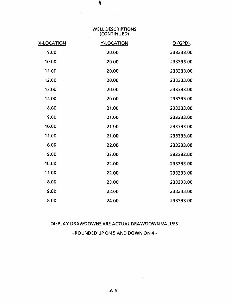
X-LOCATION
9.00
10.00
11.00
12.00
13.00
14.00
8.00
9.00
10.00
11.00
8.00
9.00
10.00
11.00
8.00
9.00
8.00
WELL DESCRIPTIONS(CONTINUED)
Y-LOCATION
20.00
20.00
20.00
20.00
20.00
20.00
21.00
21.00
21.00
21.00
22.00
22.00
22.00
22.00
23.00
23.00
24.00
Q (GPD)
233333.00
233333.00
233333.00
233333.00
233333.00
233333.00
233333.00
233333.00
233333.00
233333.00
233333.00
233333.00
233333.00
233333.00
233333.00
233333.00
233333.00
--DISPLAY DRAWDOWNS ARE ACTUAL DRAWDOWN VALUES--
--ROUNDED UP ON 5 AND DOWN ON 4--
A-5