technical evaluation of superconducting fault current ... article technical evaluation of...

energies

Article

Technical Evaluation of Superconducting FaultCurrent Limiters Used in a Micro-Grid by Consideringthe Fault Characteristics of Distributed Generation,Energy Storage and Power Loads

Lei Chen 1,*, Xiude Tu 1, Hongkun Chen 1, Jun Yang 1, Yayi Wu 1, Xin Shu 2 and Li Ren 3

1 School of Electrical Engineering, Wuhan University, Wuhan 430072, Hubei, China;[email protected] (X.T.); [email protected] (H.C.); [email protected] (J.Y.); [email protected] (Y.W.)

2 State Grid Hubei Electric Power Research Institute, Wuhan 430077, Hubei, China; [email protected] State Key Laboratory of Advanced Electromagnetic Engineering and Technology,

Huazhong University of Science and Technology, Wuhan 430074, Hubei, China; [email protected]* Correspondence: [email protected]; Tel.: +86-135-1720-5365

Academic Editor: João P. S. CatalãoReceived: 26 June 2016; Accepted: 19 September 2016; Published: 23 September 2016

Abstract: Concerning the development of a micro-grid integrated with multiple intermittentrenewable energy resources, one of the main issues is related to the improvement of its robustnessagainst short-circuit faults. In a sense, the superconducting fault current limiter (SFCL) can beregarded as a feasible approach to enhance the transient performance of a micro-grid under faultconditions. In this paper, the fault transient analysis of a micro-grid, including distributed generation,energy storage and power loads, is conducted, and regarding the application of one or moreflux-coupling-type SFCLs in the micro-grid, an integrated technical evaluation method consideringcurrent-limiting performance, bus voltage stability and device cost is proposed. In order to assess theperformance of the SFCLs and verify the effectiveness of the evaluation method, different fault casesof a 10-kV micro-grid with photovoltaic (PV), wind generator and energy storage are simulated inthe MATLAB software. The results show that, the efficient use of the SFCLs for the micro-grid cancontribute to reducing the fault current, improving the voltage sags and suppressing the frequencyfluctuations. Moreover, there will be a compromise design to fully take advantage of the SFCLparameters, and thus, the transient performance of the micro-grid can be guaranteed.

Keywords: distributed generation (DG); micro-grid; flux-coupling-type superconducting faultcurrent limiter (SFCL); technical evaluation method; short-circuit fault analyses

1. Introduction

Due to the increasing penetration of renewable distributed generation units, such as photovoltaicand wind generators, the technical idea of micro-grids has been suggested to make full use ofDG [1–6]. In addition, considering the rapid development of computer and digital communicationtechnologies [7–13], the micro-grids may play a crucial role in the future energy internet. A micro-gridis a flexible electrical system being composed of DG units, energy storage and power loads. In mostcases, the micro-grid is normally connected to the main network, unless the initial design concept ofthis micro-grid is the islanded type. When a short-circuit fault happens, the micro-grid may achievethe operation of fault ride through (FRT) or switch to the islanded mode. If the FRT operation isachieved, the micro-grid can continue to purchase power from the main network or sell power to themain network for maximize operational benefits. Once the islanded mode is triggered, the micro-gridshould maintain a reliable energy supply to customers using local DG units. Anyhow, during the

Energies 2016, 9, 769; doi:10.3390/en9100769 www.mdpi.com/journal/energies

http://www.mdpi.com/journal/energies

http://www.mdpi.com

http://www.mdpi.com/journal/energies

Energies 2016, 9, 769 2 of 21

process of the fault feeding, it is crucial to improve the micro-grid’s transient performance as muchas possible. From this perspective, the technical methods that can alleviate short-circuit current,suppress frequency/voltage fluctuations and strengthen the operational stability of the micro-grid arehelpful and useful.

The SFCL can be regarded as one of the best countermeasures to solve the problems related toa short-circuit fault. There are many remarkable merits, including: sub-cycle operation in response tofaults; reduced damage at the point of fault; and critical protection of relevant power equipment [14–19].Currently, some basic research works have been done to promote the application of one or more SFCLsin a micro-grid. In [20], a hybrid-type SFCL is applied in a simplified micro-grid with synchronous DG,and this hybrid-type SFCL’s current-limiting performance can be verified. In [21,22], the positioningof resistive-type SFCLs in direct-current (DC) and alternating-current (AC) micro-grids has beenpreliminarily discussed, and the simulation results imply that the SFCLs should be located in the directpath of current flowing from the DG units and the main network. In [23,24], the cooperative control ofSFCL and an energy storage device is suggested to improve the robustness of a micro-grid againstshort-circuit faults, and the results are able to show the effectiveness of the proposed approach.

For the application of non-superconducting FCLs in the micro-grid, a few preliminary studies havebeen done so far. In [25], a solid-state FCL based on the auto-triggered silicon control rectifier (SCR) issuggested for the micro-grid. In [26], a unidirectional FCL is used as the efficient interface betweenthe micro-grid and the main network, and this unidirectional FCL is able to improve the coordinatingperformance of the overcurrent relays configured at the micro-grid. In [27], a multi-agent-basedfault-current-limiting scheme for the micro-grid is presented, and the faulty section can be detected bythe proposed fault-location approach and is segregated using the FCLs.

Actually, regardless of the concrete type of fault current limiter, the application of current-limitingtechnologies in the micro-grid has been proven to be meaningful, and herein, SFCL is selected asthe main object for technical research. It should be noted that the employment of an SFCL in themicro-grid with intermittent renewable resources is very different from that of an SFCL in the mainnetwork, including large-scale synchronous generators. The conventional rotating electrical machinescan provide a high fault current contribution with 5 to 15-times the rating level, but as the renewableresources are generally accessed in the grid through inverters, their fault current contributions will berestrained by power electronic equipment. Thus, it may not be recommended to excessively increasethe current-limiting impedance of the SFCL used in the micro-grid.

In addition, the effects of introducing an SFCL will vary with its installation locations. There arethree common installation locations for the SFCL used in the micro-grid, and they are respectivelythe point of common coupling (PCC) between the micro-grid and the main network, the criticaltransmission line and the integration point of DG units. Concerning the differences caused by SFCLlocations, some brief explanations are provided as follows: (1) When the SFCL is installed at thePCC, it can be used to protect the entire micro-grid against the damage caused by an external fault,and the SFCL’s promising effects can be approximately classified as two kinds in accordance withthe severity (or specificity) of the external fault. One is to improve the micro-grid’s FRT capability,and the other is to make the micro-grid carry out a smooth transition between its grid-connectedand islanded modes when some permanent or serious faults occur; (2) Since the SFCL is installed atthe transmission line with an important load, it is able to improve the service stabilities of the load;(3) If the SFCL is installed at the integration point of DG units, it can be used to improve the DG’s FRTcapability, in particular under the internal fault condition. It is well known that most of the DG unitsare connected to the micro-grid through inverters, and these inverter interfaced DGs (IIDGs) havehighly variable characteristics and should meet the FRT requirements [28–31].

Considering the aforementioned individual differences related to the use of an SFCL, it is necessaryto suggest an integrated technical evaluation method to assess the overall performance of one or moreSFCLs. When these SFCLs’ current-limiting impedances, access locations and installation quantitiesare changeable, their impacts on the micro-grid’s power, voltage and frequency characteristics can be

Energies 2016, 9, 769 3 of 21

estimated. According to the comprehensive evaluation, the highly efficient transient enhancement ofthe micro-grid is beneficial to its future development.

In this paper, our research group focuses on the application of a flux-coupling-type SFCL intoa typical micro-grid with photovoltaic (PV), wind generator and energy storage and proposes a suitableevaluation method to estimate the cases in which one or more SFCLs are installed. The article isorganized in the following manner. Sections 2–4 are devoted to present the SFCL’s structural principle,discuss the fault characteristic of a typical micro-grid and propose the technical evaluation methodwhere multiple performance indexes are taken into account. In Section 5, time-domain simulationis carried out in the MATLAB software, and different fault scenarios, as well as different SFCLconfiguration schemes are simulated to verify the evaluation method’s effectiveness. In Section 6,relevant conclusions are summarized, and the next steps are suggested.

2. Presentation of the Flux-Coupling-Type SFCL

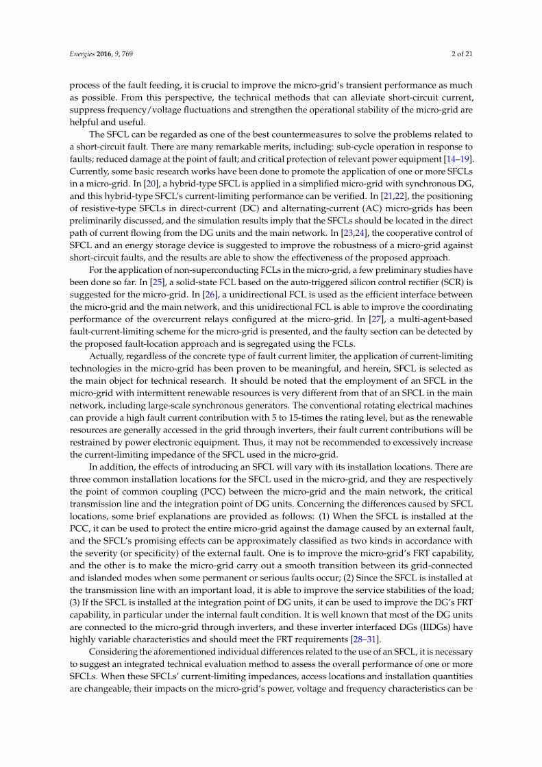
The main connection scheme of the flux-coupling-type SFCL is shown in Figure 1a [32]. This SFCLmainly consists of a coupling transformer (CT), a controlled switch Scs, a metal oxide arrester (MOA)Rmoa and a superconducting coil (SC). From the figure, L1, L2 are expressed as the CT’s self-inductances;M is the mutual inductance; Zs is the circuit impedance; Sload is the circuit load; RSC/Rmoa is expressedas the SC/MOA’s normal-state resistance. In accordance with the CT’s equivalent circuit, which iscomposed of mutual-inductance and self-inductances, the SFCL’s electrical equivalent structure isshown in Figure 1b.

Energies 2016, 9, 769 3 of 21

characteristics can be estimated. According to the comprehensive evaluation, the highly efficient

transient enhancement of the micro‐grid is beneficial to its future development.

In this paper, our research group focuses on the application of a flux‐coupling‐type SFCL into a

typical micro‐grid with photovoltaic (PV), wind generator and energy storage and proposes a

suitable evaluation method to estimate the cases in which one or more SFCLs are installed. The article

is organized in the following manner. Sections 2–4 are devoted to present the SFCL’s structural

principle, discuss the fault characteristic of a typical micro‐grid and propose the technical evaluation

method where multiple performance indexes are taken into account. In Section 5, time‐domain

simulation is carried out in the MATLAB software, and different fault scenarios, as well as different

SFCL configuration schemes are simulated to verify the evaluation method’s effectiveness. In

Section 6, relevant conclusions are summarized, and the next steps are suggested.

2. Presentation of the Flux‐Coupling‐Type SFCL

The main connection scheme of the flux‐coupling‐type SFCL is shown in Figure 1a [32]. This

SFCL mainly consists of a coupling transformer (CT), a controlled switch Scs, a metal oxide arrester

(MOA) Rmoa and a superconducting coil (SC). From the figure, L1, L2 are expressed as the CT’s

self‐inductances; M is the mutual inductance; Zs is the circuit impedance; Sload is the circuit load;

RSC/Rmoa is expressed as the SC/MOA’s normal‐state resistance. In accordance with the CT’s

equivalent circuit, which is composed of mutual‐inductance and self‐inductances, the SFCL’s

electrical equivalent structure is shown in Figure 1b.

Figure 1. Flux‐coupling‐type SFCL. (a) Main connection and (b) electrical equivalent circuit.

In the normal condition, the switch Scs is closed, and the current flowing through the SC will be lower

than its critical current. As the SC is maintained in the zero‐resistance state and non‐inductive coupling

can be achieved [33], the MOA is “short‐circuited”, and the SFCL will not affect the main circuit.

In the case that a short‐circuit fault happens, Scs will be opened rapidly, and meanwhile, the

MOA may suppress the overvoltage caused by the switching operation. Since the electromagnetic

relationship is changed by the controlled switch, the non‐inductive coupling will pass away, and also,

the fault current in the SC will cause the superconductor to be quenched. The SFCL’s current‐limiting

impedance can be calculated as: ZSFCL = [RSC + jωL2 + (knωL2)2/(Rmoa + n2ωL2), where n L L1 2= / and

k M L L1 2= / . In view of Rmoa » n2ωL2, ZSFCL ≈ RSC + jωL2 can be obtained.

Compared to the original flux‐coupling‐type SFCL, which is purely inductive [34–36], the

suggested SFCL is a resistive‐inductive‐type (hybrid type) SFCL, which can potentially bring more

positive contributions, such as inhibiting power fluctuations, restraining electromagnetic oscillations,

as well as providing critical assistance to the reliabilities and securities of power systems more

Figure 1. Flux-coupling-type SFCL. (a) Main connection and (b) electrical equivalent circuit.

In the normal condition, the switch Scs is closed, and the current flowing through the SC will belower than its critical current. As the SC is maintained in the zero-resistance state and non-inductivecoupling can be achieved [33], the MOA is “short-circuited”, and the SFCL will not affect the main circuit.

In the case that a short-circuit fault happens, Scs will be opened rapidly, and meanwhile,the MOA may suppress the overvoltage caused by the switching operation. Since the electromagneticrelationship is changed by the controlled switch, the non-inductive coupling will pass away, and also,the fault current in the SC will cause the superconductor to be quenched. The SFCL’s current-limitingimpedance can be calculated as: ZSFCL = [RSC + jωL2 + (knωL2)2/(Rmoa + n2ωL2), where n =

√L1/L2

and k = M/√

L1L2. In view of Rmoa » n2ωL2, ZSFCL ≈ RSC + jωL2 can be obtained.Compared to the original flux-coupling-type SFCL, which is purely inductive [34–36],

the suggested SFCL is a resistive-inductive-type (hybrid type) SFCL, which can potentially bring morepositive contributions, such as inhibiting power fluctuations, restraining electromagnetic oscillations,as well as providing critical assistance to the reliabilities and securities of power systems more

Energies 2016, 9, 769 4 of 21

effectively [37]. The suggested SFCL equipped with the coupling transformer and the controlled switchhas higher flexibility. Compared with the classical resistive-type SFCL being directly installed at thepower system possibly having a longer recovery time, the current flowing through the suggestedSFCL’s superconducting coil can be adjusted by changing the transformation ratio, and meanwhile,the SFCL can be put into and out of operation with greater controllability of the switch. Furthermore,the use of the coupling transformer can reduce the AC loss of the superconducting coil and avoidthe coil being directly impacted by the overcurrent at the initial time of the fault, which helps topromote the SFCL’s engineering applications in different voltage grades of electric power networks.Compared to a classical inductive-type SFCL, the SFCL’s resistive impedance can affect the generationunits’ active power characteristics more efficiently. Thus, the flux-coupling-type SFCL is suggested asthe solution to improve the transient performance of the micro-grid system.

3. Fault Characteristic Analysis of a Micro-Grid System with the Use of the SFCLs

As shown in Figure 2, the configuration structure of a typical micro-grid system is indicated,which consists of a PV generation (DG1) unit, a wind generator (DG2), an energy storage device(DG3), as well as two power loads. R1, R2, . . . R9 denote the protective relays configured in themicro-grid, and they can be used to identify and remove the short-circuit faults. As a result, the relayprotection function can be achieved. From this figure, all of the DG units are connected (or coupled)to the micro-grid through the inverters. No matter if the short-circuit fault occurs inside or outsidethe micro-grid, it is important to ensure the DG units’ transient performance. In this section, the faultcharacteristics of the PV generation, wind generator, energy storage and power loads are respectivelyanalyzed, and meanwhile, the SFCLs’ positive effects are discussed in theory.

Energies 2016, 9, 769 4 of 21

effectively [37]. The suggested SFCL equipped with the coupling transformer and the controlled

switch has higher flexibility. Compared with the classical resistive‐type SFCL being directly installed

at the power system possibly having a longer recovery time, the current flowing through the

suggested SFCL’s superconducting coil can be adjusted by changing the transformation ratio, and

meanwhile, the SFCL can be put into and out of operation with greater controllability of the switch.

Furthermore, the use of the coupling transformer can reduce the AC loss of the superconducting coil

and avoid the coil being directly impacted by the overcurrent at the initial time of the fault, which

helps to promote the SFCL’s engineering applications in different voltage grades of electric power

networks. Compared to a classical inductive‐type SFCL, the SFCL’s resistive impedance can affect

the generation units’ active power characteristics more efficiently. Thus, the flux‐coupling‐type SFCL

is suggested as the solution to improve the transient performance of the micro‐grid system.

3. Fault Characteristic Analysis of a Micro‐Grid System with the Use of the SFCLs

As shown in Figure 2, the configuration structure of a typical micro‐grid system is indicated,

which consists of a PV generation (DG1) unit, a wind generator (DG2), an energy storage device

(DG3), as well as two power loads. R1, R2,…R9 denote the protective relays configured in the

micro‐grid, and they can be used to identify and remove the short‐circuit faults. As a result, the relay

protection function can be achieved. From this figure, all of the DG units are connected (or coupled)

to the micro‐grid through the inverters. No matter if the short‐circuit fault occurs inside or outside

the micro‐grid, it is important to ensure the DG units’ transient performance. In this section, the fault

characteristics of the PV generation, wind generator, energy storage and power loads are respectively

analyzed, and meanwhile, the SFCLs’ positive effects are discussed in theory.

Figure 2. Schematic diagram of a typical micro‐grid integrated with the SFCLs. PCC, point of common coupling.

3.1. Fault Characteristic of the PV Generation

Figure 3 indicates the configuration of a PV generation connected to the micro‐grid, and herein,

the maximum power point tracking (MPPT) control is used to ensure the PV system’s operating

efficiency. The transistors VT1…VT6 denote the insulated gate bipolar transistors (IGBTs), and the

pulse‐width modulation (PWM) signals are used to drive the transistors. The overall power flowing

through the PV generation can be defined by:

Figure 2. Schematic diagram of a typical micro-grid integrated with the SFCLs. PCC, point ofcommon coupling.

3.1. Fault Characteristic of the PV Generation

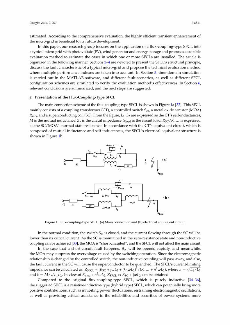
Figure 3 indicates the configuration of a PV generation connected to the micro-grid, and herein,the maximum power point tracking (MPPT) control is used to ensure the PV system’s operatingefficiency. The transistors VT1 . . . VT6 denote the insulated gate bipolar transistors (IGBTs), and the

Energies 2016, 9, 769 5 of 21

pulse-width modulation (PWM) signals are used to drive the transistors. The overall power flowingthrough the PV generation can be defined by:

PPV = PDC1 + Pg (1)

where PDC1 is the power flowing through the DC-link capacitor C1; Pg is the power inserted by theinverter to the micro-grid; PPV is the PV array output. Supposing that the power electronic converterloss can be ignored under the normal condition, PPV is approximately equal to Pg, and it is obtainedthat PPV = Pg = 3UgIg, where Ug and Ig are recorded as the nominal RMS value of phase voltage andphase current, respectively.

Energies 2016, 9, 769 5 of 21

1PV DC gP P P (1)

where PDC1 is the power flowing through the DC‐link capacitor C1; Pg is the power inserted by the

inverter to the micro‐grid; PPV is the PV array output. Supposing that the power electronic converter

loss can be ignored under the normal condition, PPV is approximately equal to Pg, and it is obtained

that PPV = Pg = 3UgIg, where Ug and Ig are recorded as the nominal RMS value of phase voltage and

phase current, respectively.

Figure 3. Schematic configuration of a grid‐connected PV generation unit for the micro‐grid.

MPPT, maximum power point tracking.

When the short‐circuit fault happens, the voltage over the PV generation unit will be

dramatically affected, and the sudden voltage drop will reduce the grid‐side power from Pg to Pgf.

Meanwhile, the DC/DC converter proceeds to transmit the PV array’s maximum output power into

the DC‐link. Owing to the power imbalance between PPV and Pgf, the DC‐link capacitance voltage will

be forced to increase sharply [38], and it can be calculated as:

21 1

1

2( 3 )= PV gf gf

DC f DCDC

P U I tV V

C

(2)

where VDC1 and VDC1−f denote the DC‐link capacitance voltage before and after the fault, and ∆t is

expressed as the duration of the fault.

In response to the PV terminal‐voltage sags, the inverter can adjust the reactive current for the

voltage support. Thus, this section also suggests the control method of the inverter for the PV system.

Regarding the voltage source inverter (VSI), which plays the role in the DC‐AC power conversion for

grid interfacing, it may use an external voltage regulator to generate the reference reactive current

Iqpv‐ref, so as to keep a stable DC‐link voltage, and herein, the reactive current’s mathematical

characteristic can be expressed as:

0 (0.9 1.1 )

(0.5 0.9 )

1 ( 0.5 )

PVq

PV PVn

PV

pu V puI= a aV pu V pu

IV pu

(3)

where the constant a is set as two and VPV is the PV voltage; Iq is the reactive current, and In is the

rated inverter current. In light of the required code, the VSI should provide full reactive current once

the PV voltage is less than 50% of the nominal rating [39]. The reference reactive current under the fault

can be determined by Iqpv‐ref = In * Iq/In, and then the active current reference Idpv‐ref can be expressed as:

Figure 3. Schematic configuration of a grid-connected PV generation unit for the micro-grid.MPPT, maximum power point tracking.

When the short-circuit fault happens, the voltage over the PV generation unit will be dramaticallyaffected, and the sudden voltage drop will reduce the grid-side power from Pg to Pgf. Meanwhile,the DC/DC converter proceeds to transmit the PV array’s maximum output power into the DC-link.Owing to the power imbalance between PPV and Pgf, the DC-link capacitance voltage will be forced toincrease sharply [38], and it can be calculated as:

VDC1− f =

√2(PPV − 3Ug f Ig f )∆t

CDC1+ V2

DC1 (2)

where VDC1 and VDC1−f denote the DC-link capacitance voltage before and after the fault, and ∆t isexpressed as the duration of the fault.

In response to the PV terminal-voltage sags, the inverter can adjust the reactive current forthe voltage support. Thus, this section also suggests the control method of the inverter for the PVsystem. Regarding the voltage source inverter (VSI), which plays the role in the DC-AC powerconversion for grid interfacing, it may use an external voltage regulator to generate the referencereactive current Iqpv-ref, so as to keep a stable DC-link voltage, and herein, the reactive current’smathematical characteristic can be expressed as:

Iq

In=

0 (0.9pu ≤ VPV ≤ 1.1pu)

a− aVPV (0.5pu ≤ VPV ≤ 0.9pu)

1 (VPV < 0.5pu)

(3)

where the constant a is set as two and VPV is the PV voltage; Iq is the reactive current, and In is the ratedinverter current. In light of the required code, the VSI should provide full reactive current once the PV

Energies 2016, 9, 769 6 of 21

voltage is less than 50% of the nominal rating [39]. The reference reactive current under the fault canbe determined by Iqpv-ref = In * Iq/In, and then the active current reference Idpv-ref can be expressed as:

Idpv−re f =

In (0.9pu ≤ VPV ≤ 1.1pu)√

I2n − I2

qpv−re f (0.5pu ≤ VPV ≤ 0.9pu)

0 (VPV < 0.5pu)

(4)

In the case that the SFCL is installed at the integration point of the DG1 and the DG2, introducingthe current-limiting impedance ZSFCL is able to compensate the voltage sags, so as to improve the PVgeneration’s FRT capability. It should also be noted that using the SFCL can reduce the requirementfor the injected reactive current of the VSI, and the SFCL’s specific behaviors will be determined by theCT’s design parameters and the superconducting coil’s rated capacity.

3.2. Fault Characteristic of the Wind Generator

As the variable-speed-type wind turbine adopting the doubly-fed induction generator (DFIG)has attracted more attention for wind generation, it is selected here to study and discuss the faultcharacteristics. Figure 4 shows the schematic diagram of a DFIG-based wind turbine connected tothe micro-grid. From the equivalent park model of the DFIG, which is based on static stator-orientedreference frame [40], the following equations are obtained.

Energies 2016, 9, 769 6 of 21

2 2

(0.9 1.1 )

(0.5 0.9 )

0 ( 0.5 )

qpv ref

n PV

dpv ref n PV

PV

I pu V pu

I = I I pu V pu

V pu

(4)

In the case that the SFCL is installed at the integration point of the DG1 and the DG2, introducing

the current‐limiting impedance ZSFCL is able to compensate the voltage sags, so as to improve the PV

generation’s FRT capability. It should also be noted that using the SFCL can reduce the requirement

for the injected reactive current of the VSI, and the SFCL’s specific behaviors will be determined by

the CT’s design parameters and the superconducting coil’s rated capacity.

3.2. Fault Characteristic of the Wind Generator

As the variable‐speed‐type wind turbine adopting the doubly‐fed induction generator (DFIG)

has attracted more attention for wind generation, it is selected here to study and discuss the fault

characteristics. Figure 4 shows the schematic diagram of a DFIG‐based wind turbine connected to the

micro‐grid. From the equivalent park model of the DFIG, which is based on static stator‐oriented

reference frame [40], the following equations are obtained.

Figure 4. Schematic diagram of a doubly‐fed induction generator (DFIG)‐based wind turbine

connected to the micro‐grid.

/s s s sV R i d dt

(5)

s s s m rL i L i

(6)

where , , , ,V i R L

are the voltage, current, magnetic flux, resistance and inductance, respectively.

Subscripts s, r, m denote the stator, rotor and mutual quantities, respectively. Assuming that the

DFIG’s terminal voltage will drop from Vs1 to Vs2 under the fault (t0 is the fault occurrence time), it

can be defined by:

j1 0

j2 0

s

s

ts

s ts

V e t tV

V e t t

(7)

Supposing that the rotor current is controlled and the rotor‐side converter keeps on working,

the rotor current is approximately constant. Its expression transferred to the stator‐side is:

jj( ) sr ttr r ri I e I e

(8)

According to constant‐linkage theorem [41], the DFIG’s stator flux before and after the fault will

be expressed as:

Figure 4. Schematic diagram of a doubly-fed induction generator (DFIG)-based wind turbine connectedto the micro-grid.

→Vs = Rs

→is + d

→ψs/dt (5)

→ψs = Ls

→is + Lm

→ir (6)

where→V,→i ,→ψ , R, L are the voltage, current, magnetic flux, resistance and inductance, respectively.

Subscripts s, r, m denote the stator, rotor and mutual quantities, respectively. Assuming that the DFIG’sterminal voltage will drop from Vs1 to Vs2 under the fault (t0 is the fault occurrence time), it can bedefined by:

→Vs =

Vs1ejωst t < t0

Vs2ejωst t ≥ t0(7)

Supposing that the rotor current is controlled and the rotor-side converter keeps on working,the rotor current is approximately constant. Its expression transferred to the stator-side is:

→ir = Irej(ωr+ω)t = Irejωst (8)

Energies 2016, 9, 769 7 of 21

According to constant-linkage theorem [41], the DFIG’s stator flux before and after the fault willbe expressed as:

→ψs =

Vs1Ls

Rs + jωsLsejωst +

RsLs Ir

Rs + jωsLsejωst t < t0

Vs2Ls

Rs + jωsLsejωst +

RsLs Ir

Rs + jωsLsejωst +

→ψ0e−

RsLs t t ≥ t0

(9)

where→ψ0 = Ls(Vs1 − Vs2)ejωst0 /(Rs + jωsLs), and it denotes the stator flux’s natural component.

By neglecting the stator resistance in Equation (9), the stator flux can be rewritten as:

→ψs =

Vs1

jωsejωst t < t0

Vs2

jωsejωst +

(Vs1 −Vs2)ejωst0

jωse−

RsLs t t ≥ t0

(10)

The stator current can be deduced by:

→is =

→ψs − Lm

→ir

Ls(11)

In the case of combining with Equations (10) and (11), the AC fault current across the DFIG’sstator winding can be calculated in:

→is =

(Vs1 −Vs2)ejωst0

jωsLse−

RsLs t +

Vs2

jωsLsejωst − Lm

→ir

Ls(12)

Since the flux-coupling-type SFCL is applied at the integration point of the DG1 and DG2,the contribution of introducing the current-limiting impedance is to compensate the generatorterminal-voltage sag and improve Ls. From Equation (12), the AC fault current flowing throughthe DFIG’s stator side can be suppressed.

3.3. Fault Characteristic of the Energy Storage

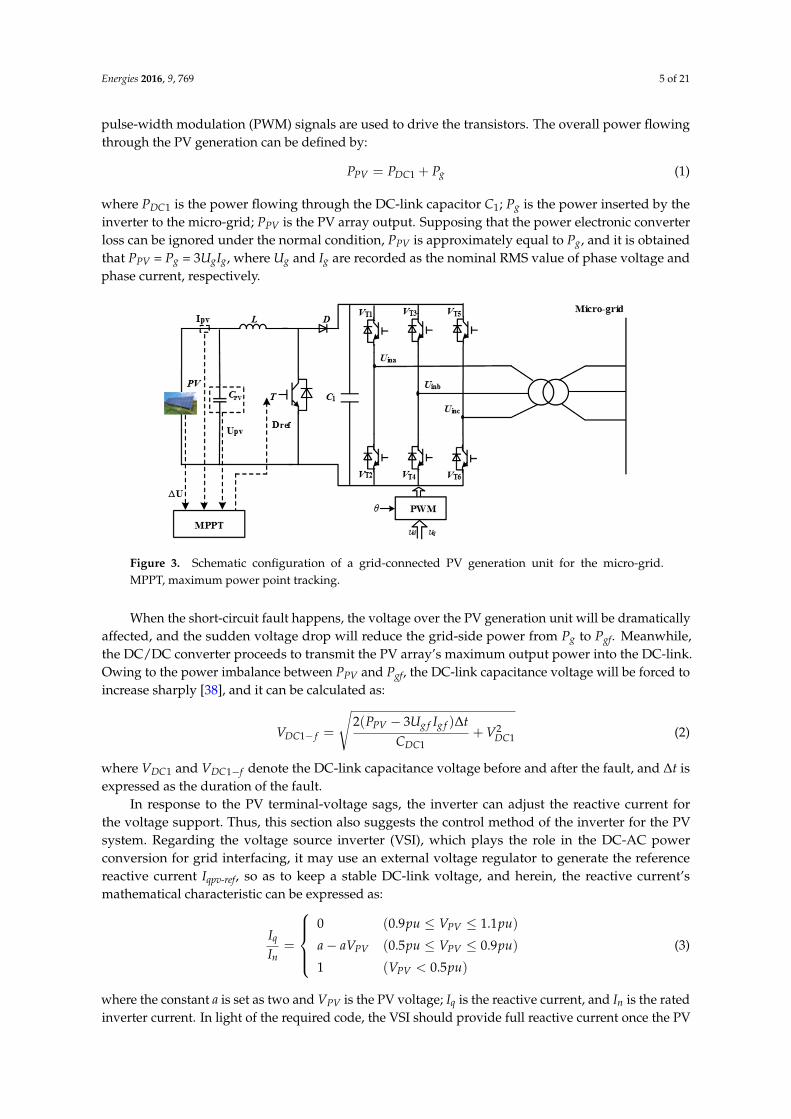
Herein, battery energy storage (DG3) is adopted to carry out the theoretical analysis, and itsfault characteristic is analyzed in brief. Commonly, the battery energy storage will switch to thevoltage-frequency (V-F) control from the original active power-reactive power (P-Q) control, when themicro-grid is undergoing a serious fault, and will switch to the islanded mode. According to thegeneral V-F control block diagram shown in Figure 5 [42], an inductor-capacitor (LC) filter is adopted,and the capacitor voltage is measured for feedback control. The control equation can be expressed as:

Pm = (kp + ks/s)(Ure f −UBE) (13)

where Pm is the power modulation factor; kp and ks are respectively the controller’s proportionalcoefficient and integral coefficient, and the proportional-integral (PI) controller is denoted in Figure 5;Uref is the reference voltage; UBE is the battery energy storage’s output voltage, which is coupled to themicro-grid. If the factor Pm is not beyond the threshold value (set as one) during the process of thefault, UBE can be quickly and effectively adjusted. In this situation, the battery energy storage can beequivalent to a constant voltage source, and UBE = Uref is achieved. If Pm is more than the thresholdvalue, the amplitude-limiting function will be activated by the converter to make Pm = 1, and thefollowing voltage equation can be obtained.

.UBE =

.EBE −

.IBEZ f (14)

where EBE is the output voltage of the energy storage converter; Zf is the equivalent impedance.

Energies 2016, 9, 769 8 of 21Energies 2016, 9, 769 8 of 21

Figure 5. General voltage‐frequency (V‐F) control block diagram for the energy storage connected to

the micro‐grid.

From Equation (14), introducing the SFCL will have no influence on the battery storage’s output

voltage in the case of Pm < 1. When Pm = 1, the voltage equation can be rewritten as:

. . .'( )BE BE BE f SFCLU E I Z Z (15)

where Z’SFCL is the SFCL’s equivalent current‐limiting impedance, which is converted from the set‐up

transformer’s high‐voltage side to the low‐voltage side.

Owing to the introduction of the flux‐coupling‐type SFCL, it has a natural function of limiting

the fault current, and during the process of current limitation, its impedance is actually connected in

series with the main circuit. Considering that the SFCL is installed near the set‐up transformer with

the energy storage unit, it can be obtained that introducing the current‐limiting impedance causes

the energy storage unit to be far away from the fault location. Thus, although the voltage sag at the

fault location cannot be avoided, the energy storage unit’s output voltage can be improved as

compared with the case without the SFCL.

3.4. Fault Characteristic of the Power Loads

Virtually all loads included in the micro‐grid system can be simulated by linear resistor‐inductor

(RL) branches. Roughly 60% of the electrical loads in distribution networks are composed of direct‐

connected induction motor (IM) loads [43]. In this paper, one of the two loads in the micro‐grid (Load

2) is regarded as the IM load, and the fault analysis is performed in brief.

For demonstration purposes, a simple mathematical representation based on a first‐order IM

model is presented, and the IM rotational speed ωfault during the fault can be expressed as [44]:

1 1( )1 1

1 1

( ) a t tfault nom

n ne

m m

(16)

where

2 2, ,

1p p fault n n fault

s IM

K V K Vm

J

,

2 2, ,

1p p fault n n fault LK V K V T

nJ

, '

3p

s IM r IM

KR

,

'

' 2 ' 2

3

[(2 ) 4( ) ]r IM

ns IM s IM r IM s IM r IM

RK

R R X X

. Herein, TL is the mechanical load torque; J is the

moment of inertia; ωs‐IM is the synchronous speed; and ωnom is the pre‐fault speed of the IM. The

parameters ' ', , ,r IM r IM s IM s IMR X R X represent the rotor resistance, rotor reactance, stator resistance

and stator reactance, respectively.

From Equation (16), the IM speed reduces exponentially with the time, and the corresponding

time constant is 1/m1. If the fault clearance time is more than 1/m1, the rotational speed might settle at

another stable rotational speed provided that the mechanical load torque is lower than the maximum

torque given from the IM torque‐speed characteristics in the fault condition. IM stalling or unstable

micro‐grid operation is most likely to occur for higher mechanical load torques and/or severe voltage

dip levels.

Considering that the flux‐coupling‐type SFCL is installed at the transmission line with Load 1,

it can help to improve the PCC voltage under the fault, compared to the PCC voltage approximately

Figure 5. General voltage-frequency (V-F) control block diagram for the energy storage connected tothe micro-grid.

From Equation (14), introducing the SFCL will have no influence on the battery storage’s outputvoltage in the case of Pm < 1. When Pm = 1, the voltage equation can be rewritten as:

.UBE =

.EBE −

.IBE(Z f + Z′SFCL) (15)

where Z′SFCL is the SFCL’s equivalent current-limiting impedance, which is converted from the set-uptransformer’s high-voltage side to the low-voltage side.

Owing to the introduction of the flux-coupling-type SFCL, it has a natural function of limitingthe fault current, and during the process of current limitation, its impedance is actually connected inseries with the main circuit. Considering that the SFCL is installed near the set-up transformer withthe energy storage unit, it can be obtained that introducing the current-limiting impedance causes theenergy storage unit to be far away from the fault location. Thus, although the voltage sag at the faultlocation cannot be avoided, the energy storage unit’s output voltage can be improved as comparedwith the case without the SFCL.

3.4. Fault Characteristic of the Power Loads

Virtually all loads included in the micro-grid system can be simulated by linear resistor-inductor(RL) branches. Roughly 60% of the electrical loads in distribution networks are composed ofdirect-connected induction motor (IM) loads [43]. In this paper, one of the two loads in the micro-grid(Load 2) is regarded as the IM load, and the fault analysis is performed in brief.

For demonstration purposes, a simple mathematical representation based on a first-order IMmodel is presented, and the IM rotational speed ωfault during the fault can be expressed as [44]:

ω f ault =n1

m1+ (ωnom −

n1

m1)e−a1(t−t1) (16)

where m1 =KpV2

p, f ault+KnV2n, f ault

Jωs−IM, n1 =

KpV2p, f ault−KnV2

n, f ault−TL

J , Kp = 3ωs−IM R′r−IM

,

Kn =3R′r−IM

ωs−IM [(2Rs−IM+R′r−IM)2+4(Xs−IM+X′r−IM)

2]. Herein, TL is the mechanical load torque; J is the

moment of inertia; ωs-IM is the synchronous speed; and ωnom is the pre-fault speed of theIM. The parameters R′r−IM, X′r−IM, Rs−IM, Xs−IM represent the rotor resistance, rotor reactance,stator resistance and stator reactance, respectively.

From Equation (16), the IM speed reduces exponentially with the time, and the correspondingtime constant is 1/m1. If the fault clearance time is more than 1/m1, the rotational speed might settle atanother stable rotational speed provided that the mechanical load torque is lower than the maximumtorque given from the IM torque-speed characteristics in the fault condition. IM stalling or unstablemicro-grid operation is most likely to occur for higher mechanical load torques and/or severe voltagedip levels.

Considering that the flux-coupling-type SFCL is installed at the transmission line with Load 1,it can help to improve the PCC voltage under the fault, compared to the PCC voltage approximately

Energies 2016, 9, 769 9 of 21

dropping to zero in the case of a serious short-circuit fault. In a sense, the improvement of the PCCvoltage can enhance the service stability of the IM load, and the requirement for the shorter faultclearance time can be properly reduced.

4. Technical Evaluation of the SFCLs Used in a Micro-Grid by Considering Multiple Indexes

In consideration of the above-mentioned individual differences related to the use of a SFCL,this section investigates an integrated technical evaluation method to assess the overall performanceof one or more SFCLs used in the micro-grid. Since the current and voltage of a micro-grid or a DGunit are the most intuitive in nature (the power and frequency characteristics can be theoreticallyanalyzed by the current and voltage), the impacts of an SFCL on them cannot be ignored. In addition,since the SFCL is used in a micro-grid whose entire capacity is relatively smaller than a large-scalemain network, it is meaningful and valuable to investigate its economics and possible effects on thegeneration cost. In sum, three crucial performance indexes, including current-limiting performance,bus voltage stability and device cost, are taken into account.

4.1. Evaluation of Current-Limiting Performance

In regard to the behaviors of an SFCL, its current-limiting performance is a key evaluationindicator with certainty. Herein, it is the first evaluation sub-function being described as:

J1 =n

∑c=1

∣∣∣∣∣ Icwithout−SFCL

Icwithout−SFCL − Ic

with−SFCL

∣∣∣∣∣ (17)

where Icwithout−SFCL and Ic

with−SFCL respectively indicate the short-circuit current at grid-bus (or DG bus)c in the case of without and with the SFCLs. In particular, the short-circuit current in the transmissionline connecting with the micro-grid and the main network may be also pointedly calculated.

4.2. Evaluation of Voltage Stability

Concerning the second evaluation sub-function, it is used to assess the SFCLs’ influence on thebus or DG voltage stability, and this sub-function is defined by:

J2 =n

∑c=1

∣∣∣∣∣ Vcnormal−state

Vcwithout−SFCL− f −Vc

with−SFCL− f

∣∣∣∣∣ (18)

where Vcwithout−SFCL− f and Vc

with−SFCL− f respectively denote the bus voltage (or the DG voltage)c under the fault in the case of without and with the SFCLs; Vc

normal−state is recorded as the bus voltage(or the DG voltage) c under the normal condition.

4.3. Evaluation of Device Cost

In consideration of the SFCL cost, it has close relations with the current-limiting impedances andthe installation number of the SFCLs, and it can be expressed as [45]:

CSFCL =NSFCL

∑i=1

ZSFCL(i) + dNSFCL + Fa (19)

where ZSFCL (i) is the current-limiting impedance of the i-th SFCL; NSFCL is the installation number;d is the cost coefficient; Fa is a penalty function.

The DG units’ generation cost can be calculated by [46]:

CDG =NDG

∑i=1

PDG−i

[

ri(1 + ri)np

(1 + ri)n − 1

](Caz−i8760ci

) + COM−i

(20)

Energies 2016, 9, 769 10 of 21

where PDG-i is the generation power of the i-th DG; ci is the capacity coefficient; np is the pay-backperiod; NDG is the number of the DG units; Caz-i and COM-i are the investment cost and maintenancecost, respectively.

The cost of the energy storage device (taking the battery storage for the research object) can becalculated by:

CES = CPPmax + CEEES + COM−ES (21)

where Pmax is the maximum power of the energy storage; EES is the rated storage energy; COM-ES isthe maintenance cost; Cp and CE are marked as the equivalent coefficients.

Accordingly, the third evaluation sub-function related to the cost analysis is defined by:

J3 =

NSFCL∑

i=1ZSFCL(i) + dNSFCL + Fa

NDG∑

i=1PDG−i

[

ri(1 + ri)n

(1 + ri)n − 1

](Caz−i8760ci

) + COM−i

+ CPPmax + CEEES + COM−ES

(22)

In the case of combining with the aforementioned three sub-functions, the integrated technicalevaluation function can be expressed as:

Jint−eva = w1 J1 + w2 J2 + w3 J3 (23)

where w1, w2, w3 are the weightings assigned to the sub-functions, which are to assess the decrease ofthe fault current, the inhibition of the voltage fluctuation and the SFCL/DG/storage cost, respectively.In a sense, the setting of the weightings should be crucial and would eventually be fixed by conditionsand experiences for the characteristics of a given system. During the following simulation analyses,different configuration schemes for the weightings are taken into account.

5. Simulation Studies and Verification

5.1. Modeling and Parameters

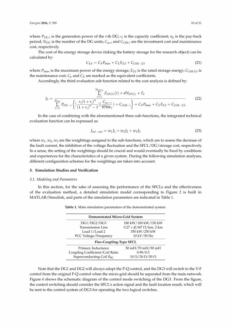
In this section, for the sake of assessing the performance of the SFCLs and the effectivenessof the evaluation method, a detailed simulation model corresponding to Figure 2 is built inMATLAB/Simulink, and parts of the simulation parameters are indicated in Table 1.

Table 1. Main simulation parameters of the demonstrated system.

Demonstrated Micro-Grid System

DG1/DG2/DG3 180 kW/100 kW/150 kWTransmission Line 0.27 + j0.347 Ω/km, 2 km

Load 1/Load 2 350 kW/250 kWPCC Voltage/Frequency 10 kV/50 Hz

Flux-Coupling-Type SFCL

Primary Inductance 50 mH/70 mH/90 mHCoupling Coefficient/Coil Ratio 0.99/0.5

Superconducting Coil RSC 10 Ω/30 Ω/50 Ω

Note that the DG1 and DG2 will always adopt the P-Q control, and the DG3 will switch to the V-Fcontrol from the original P-Q control when the micro-grid should be separated from the main network.Figure 6 shows the schematic diagram of the control mode switching of the DG3. From the figure,the control switching should consider the SFCL’s action signal and the fault location result, which willbe sent to the control system of DG3 for operating the two logical switches.

Energies 2016, 9, 769 11 of 21

Energies 2016, 9, 769 11 of 21

Figure 6. Control mode switching of the battery energy storage (DG3).

During the simulation, the SFCL’s controlled switch is simulated by an anti‐parallel IGBT pairs,

and the coupling transformer is based on a standard transformer model from the MATLAB model

library. The quench/recovery model of the superconducting coil is according to Figure 7 [47], and the

SC’s operating characteristic can be expressed as:

0

10 2

0 1

1 1 1 1 2

2 2 2 2

0 ( )

[1 exp( )] ( )( )

( ) ( )

( ) ( )

n

t t

t tR t t t

R t =a t t b t t t

a t t b t t

(24)

where Rn denotes the SFCL’s normal‐state resistance; τ is the time constant. The SFCL’s time‐domain

characteristic is stated such that t0, t1 and t2 indicate the quench‐starting time, the first recovery‐

starting time and the secondary recovery‐starting time, respectively. a1, b1, a2 and b2 are respectively

the function coefficients. It is assumed that the SC will enter the quenching state within 4 ms, and

after the short‐circuit fault is removed, the SC’s recovery time is set as 0.5 s to cooperate with

the reclosing.

Figure 7. Quench/recovery of the superconducting coil used in the SFCL.

As shown in Figure 8, different FRT curves of a defined stay‐connected time for IIDG are

indicated [48,49]. From this figure, the FRT requirement differs from one standard to the other based

on the countries’ grid code. During the simulations, the Denmark code is selectively used, and in the

case that the grid voltage drops to 20% of the nominal level, the IIDG should remain in the

grid‐connected state for a duration of 150 ms.


During the simulation, the SFCL’s controlled switch is simulated by an anti-parallel IGBT pairs,and the coupling transformer is based on a standard transformer model from the MATLAB modellibrary. The quench/recovery model of the superconducting coil is according to Figure 7 [47], and theSC’s operating characteristic can be expressed as:

R(t) =

0 (t < t0)

Rn[1− exp(− t− t0

τ)]

1/2

(t0 ≤ t < t1)

a1(t− t1) + b1 (t1 ≤ t < t2)

a2(t− t2) + b2 (t2 ≤ t)

(24)

where Rn denotes the SFCL’s normal-state resistance; τ is the time constant. The SFCL’s time-domaincharacteristic is stated such that t0, t1 and t2 indicate the quench-starting time, the first recovery-startingtime and the secondary recovery-starting time, respectively. a1, b1, a2 and b2 are respectively thefunction coefficients. It is assumed that the SC will enter the quenching state within 4 ms, and after theshort-circuit fault is removed, the SC’s recovery time is set as 0.5 s to cooperate with the reclosing.

Energies 2016, 9, 769 11 of 21


During the simulation, the SFCL’s controlled switch is simulated by an anti‐parallel IGBT pairs,

and the coupling transformer is based on a standard transformer model from the MATLAB model

library. The quench/recovery model of the superconducting coil is according to Figure 7 [47], and the

SC’s operating characteristic can be expressed as:

0

10 2

0 1

1 1 1 1 2

2 2 2 2

0 ( )

[1 exp( )] ( )( )

( ) ( )

( ) ( )

n

t t

t tR t t t

R t =a t t b t t t

a t t b t t

(24)

where Rn denotes the SFCL’s normal‐state resistance; τ is the time constant. The SFCL’s time‐domain

characteristic is stated such that t0, t1 and t2 indicate the quench‐starting time, the first recovery‐

starting time and the secondary recovery‐starting time, respectively. a1, b1, a2 and b2 are respectively

the function coefficients. It is assumed that the SC will enter the quenching state within 4 ms, and

after the short‐circuit fault is removed, the SC’s recovery time is set as 0.5 s to cooperate with

the reclosing.


As shown in Figure 8, different FRT curves of a defined stay‐connected time for IIDG are

indicated [48,49]. From this figure, the FRT requirement differs from one standard to the other based

on the countries’ grid code. During the simulations, the Denmark code is selectively used, and in the

case that the grid voltage drops to 20% of the nominal level, the IIDG should remain in the

grid‐connected state for a duration of 150 ms.


As shown in Figure 8, different FRT curves of a defined stay-connected time for IIDG areindicated [48,49]. From this figure, the FRT requirement differs from one standard to the other based onthe countries’ grid code. During the simulations, the Denmark code is selectively used, and in the casethat the grid voltage drops to 20% of the nominal level, the IIDG should remain in the grid-connectedstate for a duration of 150 ms.

Energies 2016, 9, 769 12 of 21

Energies 2016, 9, 769 12 of 21

Figure 8. Different fault ride through (FRT) curves of a defined stay‐connected time for the inverter

interfaced DG (IIDG).

In addition, based on the consideration of a simplified analysis, the DG1, DG2 and DG3 are

physically connected to the same inverter bus during the simulations, and accordingly, the

installation number of the SFCLs can be appropriately reduced. In the following analyses, the external

fault (F1 point) and the internal fault (F2 point) are both simulated, and the computed results of the

evaluation function are also given.

5.2. Simulations of the External Fault (F1 Point)

In the normal (no fault) condition, the energy storage device’s effects on eliminating the power

fluctuations caused by the intermittent energy sources are taken into account, and the DGs’ overall

active power will be controlled as 300 kW (PDG1 + PDG2 + PDG3 = 300 kW). In other words, the

micro‐grid’s power shortage with the capacity value of 300 kW will be supported by the main

network. Furthermore, the simulation conditions of the external fault (F1 point) are described as a

three‐phase ground fault happening at t = 1 s; the fault resistance is 1 Ω; the duration of the fault is

0.2 s. In regard to this fault case, only one SFCL is installed at the PCC, and it is expected to protect

the entire micro‐grid system from the fault damage.

Different SFCL parameters are also considered, and Figure 9 shows the fault current flowing

from the micro‐grid side to the PCC (taking the A‐phase as an example). The SFCL’s current‐limiting

effects will become more obvious along with the increase of the SFCL parameters, but since the fault

current is mainly contributed by the DG units, the maximum amplitude of the fault current will

generally not reach a very high level. From this perspective, it may not be necessary to excessively

increase the SFCL parameters.

Figure 9. Fault current from the micro‐grid side to the PCC under the external fault (A‐phase).

Figure 10 shows the micro‐grid’s PCC voltage under the external fault (A‐phase). From this

figure, the PCC voltage will be down to 53% of the nominal level in the case of without SFCL. Once

0.9 0.95 1 1.05 1.1

-60

-40

-20

0

20

40

60

Time (s)

i pcc (

A)

without SFCLL1 = 50 mH and Rsc = 10 Ω

L1 = 70 mH and Rsc = 30 Ω


Figure 8. Different fault ride through (FRT) curves of a defined stay-connected time for the inverterinterfaced DG (IIDG).

In addition, based on the consideration of a simplified analysis, the DG1, DG2 and DG3 arephysically connected to the same inverter bus during the simulations, and accordingly, the installationnumber of the SFCLs can be appropriately reduced. In the following analyses, the external fault(F1 point) and the internal fault (F2 point) are both simulated, and the computed results of theevaluation function are also given.


In the normal (no fault) condition, the energy storage device’s effects on eliminating thepower fluctuations caused by the intermittent energy sources are taken into account, and the DGs’overall active power will be controlled as 300 kW (PDG1 + PDG2 + PDG3 = 300 kW). In other words,the micro-grid’s power shortage with the capacity value of 300 kW will be supported by the mainnetwork. Furthermore, the simulation conditions of the external fault (F1 point) are described asa three-phase ground fault happening at t = 1 s; the fault resistance is 1 Ω; the duration of the fault is0.2 s. In regard to this fault case, only one SFCL is installed at the PCC, and it is expected to protect theentire micro-grid system from the fault damage.

Different SFCL parameters are also considered, and Figure 9 shows the fault current flowing fromthe micro-grid side to the PCC (taking the A-phase as an example). The SFCL’s current-limiting effectswill become more obvious along with the increase of the SFCL parameters, but since the fault currentis mainly contributed by the DG units, the maximum amplitude of the fault current will generallynot reach a very high level. From this perspective, it may not be necessary to excessively increase theSFCL parameters.

Energies 2016, 9, 769 12 of 21

Figure 8. Different fault ride through (FRT) curves of a defined stay‐connected time for the inverter

interfaced DG (IIDG).

In addition, based on the consideration of a simplified analysis, the DG1, DG2 and DG3 are

physically connected to the same inverter bus during the simulations, and accordingly, the

installation number of the SFCLs can be appropriately reduced. In the following analyses, the external

fault (F1 point) and the internal fault (F2 point) are both simulated, and the computed results of the

evaluation function are also given.


In the normal (no fault) condition, the energy storage device’s effects on eliminating the power

fluctuations caused by the intermittent energy sources are taken into account, and the DGs’ overall

active power will be controlled as 300 kW (PDG1 + PDG2 + PDG3 = 300 kW). In other words, the

micro‐grid’s power shortage with the capacity value of 300 kW will be supported by the main

network. Furthermore, the simulation conditions of the external fault (F1 point) are described as a

three‐phase ground fault happening at t = 1 s; the fault resistance is 1 Ω; the duration of the fault is

0.2 s. In regard to this fault case, only one SFCL is installed at the PCC, and it is expected to protect

the entire micro‐grid system from the fault damage.

Different SFCL parameters are also considered, and Figure 9 shows the fault current flowing

from the micro‐grid side to the PCC (taking the A‐phase as an example). The SFCL’s current‐limiting

effects will become more obvious along with the increase of the SFCL parameters, but since the fault

current is mainly contributed by the DG units, the maximum amplitude of the fault current will

generally not reach a very high level. From this perspective, it may not be necessary to excessively

increase the SFCL parameters.

Figure 9. Fault current from the micro‐grid side to the PCC under the external fault (A‐phase).

Figure 10 shows the micro‐grid’s PCC voltage under the external fault (A‐phase). From this

figure, the PCC voltage will be down to 53% of the nominal level in the case of without SFCL. Once

0.9 0.95 1 1.05 1.1

-60

-40

-20

0

20

40

60

Time (s)

i pcc (

A)




Figure 9. Fault current from the micro-grid side to the PCC under the external fault (A-phase).

Energies 2016, 9, 769 13 of 21

Figure 10 shows the micro-grid’s PCC voltage under the external fault (A-phase). From this figure,the PCC voltage will be down to 53% of the nominal level in the case of without SFCL. Once theflux-coupling-type SFCL is employed, the PCC voltage can be even improved to 82% of the nominallevel, and it is conducive to enhance the FRT capabilities of the IIDG units. Figures 11–13 show theexchange power and frequency response of the micro-grid system under the external fault. Before themicro-grid is forced to be disconnected from the main network at t = 1.13 s, the voltage drop at thePCC will greatly affect the power exchange.

Energies 2016, 9, 769 13 of 21

the flux‐coupling‐type SFCL is employed, the PCC voltage can be even improved to 82% of the

nominal level, and it is conducive to enhance the FRT capabilities of the IIDG units. Figures 11–13

show the exchange power and frequency response of the micro‐grid system under the external fault.

Before the micro‐grid is forced to be disconnected from the main network at t = 1.13 s, the voltage

drop at the PCC will greatly affect the power exchange.

Figure 10. PCC voltage characteristic of the micro‐grid system under the external fault (A‐phase).

Figure 11. Active power of the micro‐grid at the PCC under the external fault.

Figure 12. Reactive power of the micro‐grid at the PCC under the external fault.

0.9 0.95 1 1.05 1.1-12

-8

-4

0

4

8

12

Time (s)

Vpc

c (kV

)




0.8 0.9 1 1.1 1.2 1.3-600

-400

-200

0

200

400

600

Time (s)

Pex

( kW

)




0.8 0.9 1 1.1 1.2 1.3-600

-400

-200

0

200

400

600

Time (s)

Qex

( kv

ar)




Figure 10. PCC voltage characteristic of the micro-grid system under the external fault (A-phase).

Energies 2016, 9, 769 13 of 21









0.9 0.95 1 1.05 1.1-12

-8

-4

0

4

8

12

Time (s)

Vpc

c (kV

)




0.8 0.9 1 1.1 1.2 1.3-600

-400

-200

0

200

400

600

Time (s)

Pex

( kW

)




0.8 0.9 1 1.1 1.2 1.3-600

-400

-200

0

200

400

600

Time (s)

Qex

( kv

ar)




Figure 11. Active power of the micro-grid at the PCC under the external fault.

Energies 2016, 9, 769 13 of 21









0.9 0.95 1 1.05 1.1-12

-8

-4

0

4

8

12

Time (s)

Vpc

c (kV

)




0.8 0.9 1 1.1 1.2 1.3-600

-400

-200

0

200

400

600

Time (s)

Pex

( kW

)




0.8 0.9 1 1.1 1.2 1.3-600

-400

-200

0

200

400

600

Time (s)

Qex

( kv

ar)




Figure 12. Reactive power of the micro-grid at the PCC under the external fault.


Figure 13. Frequency fluctuations of the micro‐grid under the external fault.

Regarding the setting of the disconnection time, a brief explanation is given. When the external

fault occurs, the disconnection time of the micro‐grid will closely depend on the relay protection’s

algorithm strategy and the PCC switch’s response speed. In this paper, according to a general

protection configuration method used in the power distribution network, the directional overcurrent

protection can be appreciatively used in the micro‐grid, and once the fault current flowing through

the PCC meets the setting conditions, the relay protection (R1) will trip off the PCC switch to separate

the micro‐grid under the external fault. For R2–R9, they can be used to deal with the internal fault.

From the literature [50–52], the whole action time of the directional overcurrent protection can be

reduced to 6–7 fundamental‐frequency cycles in the case that the protection parameters are properly

set. Therefore, the disconnection is supposed to be effective at t = 1.13 s, and namely, the islanded

mode will be activated at 130 ms after the fault.

After the fault occurs, the exchange power’s flowing direction will be reversed, and the

micro‐grid will transmit power energy to the main network. Owing to the use of the SFCL, the

fluctuating margin of the exchange power can be reduced to a certain extent. Moreover, the

micro‐grid frequency’s fluctuating margin is about 0.18 Hz in the case of without SFCL, and it may

be suppressed within the level of 0.09 Hz when the SFCL is employed.

According to the simulation results, each of the three evaluation sub‐functions will be calculated,

and herein, some of the calculation parameters are listed: the commercial superconducting tapes have

a high resistivity matrix with a linear resistance of 0.354 Ω/m, and the tape cost is 70 $/m; the

generating costs of the wind power and the photovoltaic DG are respectively set as 1283.697 $/kW

and 2384.8514 $/kW [53]; in regard to the cost of the energy storage device, Cp = 426 $/kW,

CE = 180 $/Ah and Com‐ES = 13.5 $/kW [54]. Herein, the battery cost parameters are suitable for the

vanadium redox flow battery (VRFB), and its rated voltage is set as 800 V. In accordance with those

different current‐limiting parameters of the SFCL, the calculation results of the three evaluation

sub‐functions are shown in Table 2.

Table 2. Calculation results of the three evaluation sub‐functions under different current‐limiting

parameters (external fault).

Current‐Limiting Parameters Evaluation Sub‐functions

J1 J2 J3

L1 = 50 mH and Rsc = 10 Ω 20.9013 25.4615 5.5087

L1 = 70 mH and Rsc = 30 Ω 17.2433 18.6047 10.504

L1 = 90 mH and Rsc = 50 Ω 14.6096 16.0384 14.8169

For the calculation of the integrated technical evaluation function (Jint‐eva), the setting of the

weightings w1, w2, w3 will be critical, and herein, four typical allocation schemes are taken into account.

The detailed calculation results are shown in Table 3. The change of the weightings will closely

0.9 0.95 1 1.05 1.149.7

49.8

49.9

50

50.1

50.2

50.3

Time (s)

f (H

z)

without SFCLL

1= 50 mH and R

sc= 10 Ω

L1 = 70 mH and R sc = 30 Ω

L1 = 90 mH and R sc = 50 Ω

Figure 13. Frequency fluctuations of the micro-grid under the external fault.

Regarding the setting of the disconnection time, a brief explanation is given. When the externalfault occurs, the disconnection time of the micro-grid will closely depend on the relay protection’salgorithm strategy and the PCC switch’s response speed. In this paper, according to a general protectionconfiguration method used in the power distribution network, the directional overcurrent protectioncan be appreciatively used in the micro-grid, and once the fault current flowing through the PCCmeets the setting conditions, the relay protection (R1) will trip off the PCC switch to separate themicro-grid under the external fault. For R2–R9, they can be used to deal with the internal fault.From the literature [50–52], the whole action time of the directional overcurrent protection can bereduced to 6–7 fundamental-frequency cycles in the case that the protection parameters are properlyset. Therefore, the disconnection is supposed to be effective at t = 1.13 s, and namely, the islandedmode will be activated at 130 ms after the fault.

After the fault occurs, the exchange power’s flowing direction will be reversed, and the micro-gridwill transmit power energy to the main network. Owing to the use of the SFCL, the fluctuating marginof the exchange power can be reduced to a certain extent. Moreover, the micro-grid frequency’sfluctuating margin is about 0.18 Hz in the case of without SFCL, and it may be suppressed within thelevel of 0.09 Hz when the SFCL is employed.

According to the simulation results, each of the three evaluation sub-functions will be calculated,and herein, some of the calculation parameters are listed: the commercial superconducting tapeshave a high resistivity matrix with a linear resistance of 0.354 Ω/m, and the tape cost is 70 $/m;the generating costs of the wind power and the photovoltaic DG are respectively set as 1283.697 $/kWand 2384.8514 $/kW [53]; in regard to the cost of the energy storage device, Cp = 426 $/kW,CE = 180 $/Ah and Com-ES = 13.5 $/kW [54]. Herein, the battery cost parameters are suitable forthe vanadium redox flow battery (VRFB), and its rated voltage is set as 800 V. In accordance withthose different current-limiting parameters of the SFCL, the calculation results of the three evaluationsub-functions are shown in Table 2.

Table 2. Calculation results of the three evaluation sub-functions under different current-limitingparameters (external fault).

Current-Limiting ParametersEvaluation Sub-Functions

J1 J2 J3

L1 = 50 mH and Rsc = 10 Ω 20.9013 25.4615 5.5087L1 = 70 mH and Rsc = 30 Ω 17.2433 18.6047 10.504L1 = 90 mH and Rsc = 50 Ω 14.6096 16.0384 14.8169

Energies 2016, 9, 769 15 of 21

For the calculation of the integrated technical evaluation function (Jint-eva), the setting of theweightings w1, w2, w3 will be critical, and herein, four typical allocation schemes are taken into account.The detailed calculation results are shown in Table 3. The change of the weightings will closelydetermine the final numerical value of the evaluation function. In addition, along with the augment ofthe SFCL’s current-limiting parameters, the function value will decrease at first then increase under thecondition of w1 = 0.3, w2 = 0.3, w3 = 0.4. When the function value is smaller, the SFCL’s comprehensiveperformance behaviors will be better. It may be inferred that there will be a compromise design for theSFCL parameters to fully obtain the performance advantages.

Table 3. Calculation results of the integrated technical evaluation function under different weightingfactors (external fault).

Current-LimitingParameters

Integrated Technical Evaluation Function (Jint-eva)

w1 = 0.1,w2 = 0.1,w3 = 0.8

w1 = 0.1,w2 = 0.8,w3 = 0.1

w1 = 0.8,w2 = 0.1,w3 = 0.1

w1 = 0.3,w2 = 0.3,w3 = 0.4

L1 = 50 mH and Rsc = 10 Ω 9.0432 23.0102 19.8181 16.1123L1 = 70 mH and Rsc = 30 Ω 11.9882 17.6585 16.7055 14.9561L1 = 90 mH and Rsc = 50 Ω 14.9183 15.7734 14.7732 15.1212

Noted that this conclusion will be effective when the three weightings have similar values orhave a little difference, and in general, it may not be recommended to excessively emphasize a certainweighting since the other weightings will lose their importance and significance [55]. In addition,if the proposed technical evaluation function is used to optimally select and place the SFCLs in themicro-grid, the optimization objective is to make the integrated function value be the smallest, and theSFCLs’ current-limiting impedances, access locations and installation quantities will be constrained bycertain conditions. Due to the use of an intelligent algorithm, such as particle swarm optimization(PSO) [56,57], the optimization results can be selectively obtained. As this paper’s main objective is todo the technical evaluation and provide a quantitative comparison, the detailed optimization workswill be performed and reported in later articles.

5.3. Simulations of the Internal Fault (F2 Point)

When the internal fault happens at the F2 point, it is expected to improve the micro-grid’s FRTcapability. Under this fault, the micro-grid system does not have to disconnect from the main network,in particular when the power exchange is considerable. During the transient simulations, two SFCLsare employed. One of them is installed at the integration point of the DG units, and the other isinstalled at the PCC. The two SFCLs are respectively used to limit the fault contributions from the DGunits and the main network, and their parameters are supposed to be the same as each other.

For the internal fault, the fault occurrence time is t = 1 s; the fault resistance is 1 Ω; the durationof the fault is 0.2 s. Figures 14 and 15 show the waveforms of the fault currents contributed by theDG units and the main network, respectively. From the figures, using the SFCLs, one is able to limitthe fault currents within acceptable levels. Herein, the fault current in the PCC is selected for dataanalysis. The fault current’s peak value will rise to 740 A without the SFCL. Since the SFCL parametersare respectively set as L1 = 50 mH and Rsc = 10 Ω, L1 = 70 mH and Rsc = 30 Ω, L1 = 90 mH andRsc = 50 Ω, the fault current’s peak value can be respectively suppressed to 180 A, 117 A, 89 A, and thecurrent-limiting ratio is about 75.7%, 84.2%, 88%.


Figure 14. Fault current contributed by the DG units under the internal fault (A‐phase).

Figure 15. Fault current provided by the main network under the internal fault (A‐phase).

Figure 16. Voltage at the integration point of the DG units under the internal fault (A‐phase).

Figures 16–19 show the DG voltage, exchange power and frequency fluctuations of the

micro‐grid system under the internal fault. From these figures, the positive effects of the two SFCLs can

be observed. In the case of without the SFCL, the main network will sell an amount of active power and

reactive power to the main network under the fault, and the power fluctuations will be very obvious.

Along with the increase of the SFCLs’ current‐limiting parameters, the exchange power will be reduced

to be lower than the normal level. Since the power Load 1 is shorted, the decrease of the exchange power

and the full utilization of the local DG units can help to achieve the power balance. In addition, taking

the enhancement of the micro‐grid’s frequency stability as an example, employing the SFCLs can make

0.9 0.95 1 1.05 1.1-50

0

50

100

Time (s)

i DG

-tot

al (

A)




0.9 0.95 1 1.05 1.1-800

-600

-400

-200

0

200

400

600

800

Time (s)

i pcc (

A)




0.9 0.95 1 1.05 1.1-12

-8

-4

0

4

8

12

Time (s)

VD

G (

kV)




Figure 14. Fault current contributed by the DG units under the internal fault (A-phase).

Energies 2016, 9, 769 16 of 21












0.9 0.95 1 1.05 1.1-50

0

50

100

Time (s)

i DG

-tot

al (

A)




0.9 0.95 1 1.05 1.1-800

-600

-400

-200

0

200

400

600

800

Time (s)

i pcc (

A)




0.9 0.95 1 1.05 1.1-12

-8

-4

0

4

8

12

Time (s)

VD

G (

kV)




Figure 15. Fault current provided by the main network under the internal fault (A-phase).

Energies 2016, 9, 769 16 of 21












0.9 0.95 1 1.05 1.1-50

0

50

100

Time (s)

i DG

-tot

al (

A)




0.9 0.95 1 1.05 1.1-800

-600

-400

-200

0

200

400

600

800

Time (s)

i pcc (

A)




0.9 0.95 1 1.05 1.1-12

-8

-4

0

4

8

12

Time (s)

VD

G (

kV)




Figure 16. Voltage at the integration point of the DG units under the internal fault (A-phase).

Figures 16–19 show the DG voltage, exchange power and frequency fluctuations of the micro-gridsystem under the internal fault. From these figures, the positive effects of the two SFCLs can beobserved. In the case of without the SFCL, the main network will sell an amount of active power andreactive power to the main network under the fault, and the power fluctuations will be very obvious.Along with the increase of the SFCLs’ current-limiting parameters, the exchange power will be reducedto be lower than the normal level. Since the power Load 1 is shorted, the decrease of the exchangepower and the full utilization of the local DG units can help to achieve the power balance. In addition,

Energies 2016, 9, 769 17 of 21

taking the enhancement of the micro-grid’s frequency stability as an example, employing the SFCLscan make the fluctuating margin of the micro-grid frequency limited within 0.11 Hz, compared to itrising to 0.62 Hz under the condition without the SFCL.

Energies 2016, 9, 769 17 of 21

the fluctuating margin of the micro‐grid frequency limited within 0.11 Hz, compared to it rising to 0.62

Hz under the condition without the SFCL.

Figure 17. Active power of the micro‐grid at the PCC under the internal fault.

Figure 18. Reactive power of the micro‐grid at the PCC under the internal fault.

Figure 19. Frequency fluctuations of the micro‐grid under the internal fault.

In a similar way, the calculation results of the three evaluation sub‐functions are shown in

Table 4, and the analysis results of the integrated technical evaluation function under different

weighting factors are shown in Table 5. For the weightings set as w1 = 0.3, w2 = 0.3, w3 = 0.4, the current‐

limiting parameters of L1 = 70 mH and Rsc = 30 Ω can be regarded as the most suitable of the three

demonstrative schemes.

0.8 0.9 1 1.1 1.2 1.30

200

400

600

800

1000

1200

1400

1600

1800

2000

Time (s)

Pex

( kW

)




0.8 0.9 1 1.1 1.2 1.3-200

0

200

400

600

800

1000

Time (s)

Qex

( kv

ar)




0.9 0.95 1 1.05 1.149.5

50

50.5

51

Time (s)

f (H

z)




Figure 17. Active power of the micro-grid at the PCC under the internal fault.

Energies 2016, 9, 769 17 of 21











0.8 0.9 1 1.1 1.2 1.30

200

400

600

800

1000

1200

1400

1600

1800

2000

Time (s)

Pex

( kW

)




0.8 0.9 1 1.1 1.2 1.3-200

0

200

400

600

800

1000

Time (s)

Qex

( kv

ar)




0.9 0.95 1 1.05 1.149.5

50

50.5

51

Time (s)

f (H

z)




Figure 18. Reactive power of the micro-grid at the PCC under the internal fault.

Energies 2016, 9, 769 17 of 21











0.8 0.9 1 1.1 1.2 1.30

200

400

600

800

1000

1200

1400

1600

1800

2000

Time (s)

Pex

( kW

)




0.8 0.9 1 1.1 1.2 1.3-200

0

200

400

600

800

1000

Time (s)

Qex

( kv

ar)




0.9 0.95 1 1.05 1.149.5

50

50.5

51

Time (s)

f (H

z)




Figure 19. Frequency fluctuations of the micro-grid under the internal fault.

In a similar way, the calculation results of the three evaluation sub-functions are shown inTable 4, and the analysis results of the integrated technical evaluation function under differentweighting factors are shown in Table 5. For the weightings set as w1 = 0.3, w2 = 0.3, w3 = 0.4,the current-limiting parameters of L1 = 70 mH and Rsc = 30 Ω can be regarded as the most suitable ofthe three demonstrative schemes.

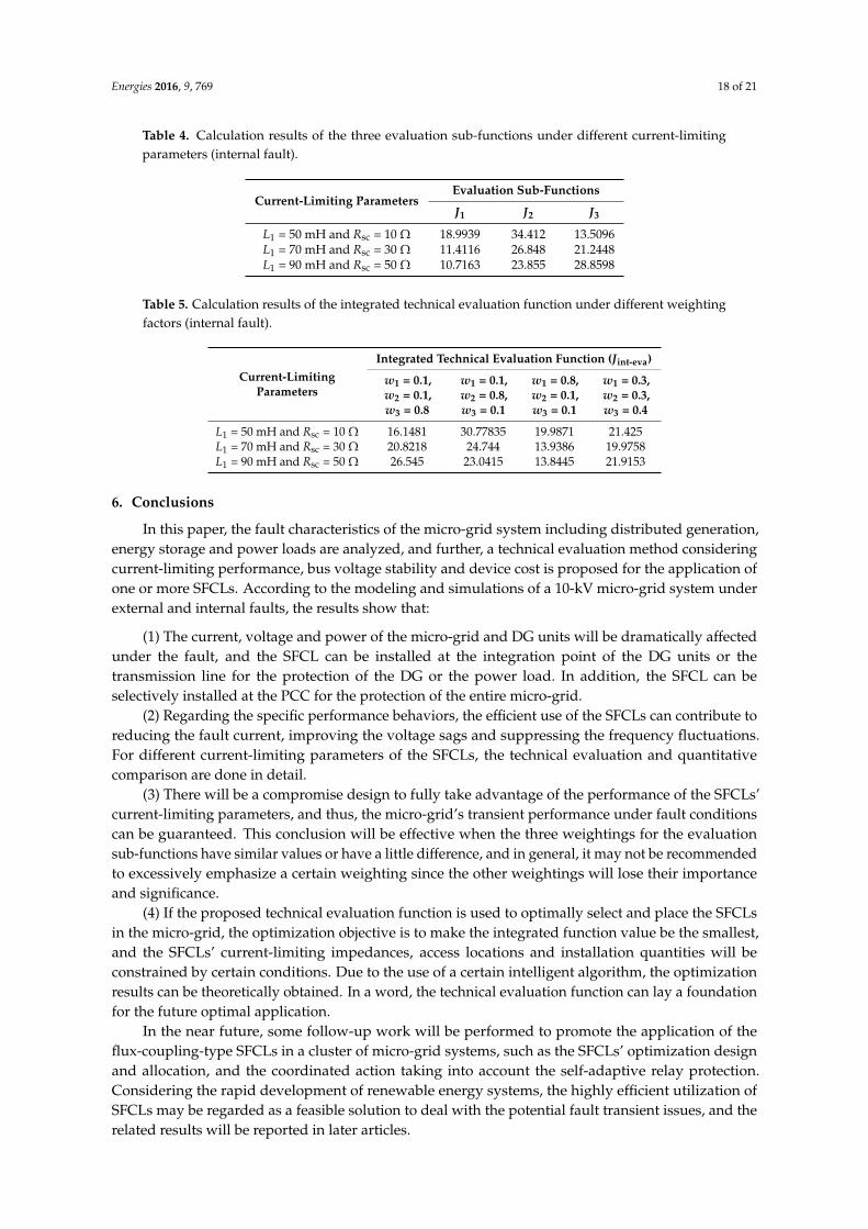
Energies 2016, 9, 769 18 of 21

Table 4. Calculation results of the three evaluation sub-functions under different current-limitingparameters (internal fault).

Current-Limiting ParametersEvaluation Sub-Functions

J1 J2 J3

L1 = 50 mH and Rsc = 10 Ω 18.9939 34.412 13.5096L1 = 70 mH and Rsc = 30 Ω 11.4116 26.848 21.2448L1 = 90 mH and Rsc = 50 Ω 10.7163 23.855 28.8598

Table 5. Calculation results of the integrated technical evaluation function under different weightingfactors (internal fault).

Current-LimitingParameters

Integrated Technical Evaluation Function (Jint-eva)

w1 = 0.1,w2 = 0.1,w3 = 0.8

w1 = 0.1,w2 = 0.8,w3 = 0.1

w1 = 0.8,w2 = 0.1,w3 = 0.1

w1 = 0.3,w2 = 0.3,w3 = 0.4

L1 = 50 mH and Rsc = 10 Ω 16.1481 30.77835 19.9871 21.425L1 = 70 mH and Rsc = 30 Ω 20.8218 24.744 13.9386 19.9758L1 = 90 mH and Rsc = 50 Ω 26.545 23.0415 13.8445 21.9153

6. Conclusions

In this paper, the fault characteristics of the micro-grid system including distributed generation,energy storage and power loads are analyzed, and further, a technical evaluation method consideringcurrent-limiting performance, bus voltage stability and device cost is proposed for the application ofone or more SFCLs. According to the modeling and simulations of a 10-kV micro-grid system underexternal and internal faults, the results show that:

(1) The current, voltage and power of the micro-grid and DG units will be dramatically affectedunder the fault, and the SFCL can be installed at the integration point of the DG units or thetransmission line for the protection of the DG or the power load. In addition, the SFCL can beselectively installed at the PCC for the protection of the entire micro-grid.

(2) Regarding the specific performance behaviors, the efficient use of the SFCLs can contribute toreducing the fault current, improving the voltage sags and suppressing the frequency fluctuations.For different current-limiting parameters of the SFCLs, the technical evaluation and quantitativecomparison are done in detail.

(3) There will be a compromise design to fully take advantage of the performance of the SFCLs’current-limiting parameters, and thus, the micro-grid’s transient performance under fault conditionscan be guaranteed. This conclusion will be effective when the three weightings for the evaluationsub-functions have similar values or have a little difference, and in general, it may not be recommendedto excessively emphasize a certain weighting since the other weightings will lose their importanceand significance.

(4) If the proposed technical evaluation function is used to optimally select and place the SFCLsin the micro-grid, the optimization objective is to make the integrated function value be the smallest,and the SFCLs’ current-limiting impedances, access locations and installation quantities will beconstrained by certain conditions. Due to the use of a certain intelligent algorithm, the optimizationresults can be theoretically obtained. In a word, the technical evaluation function can lay a foundationfor the future optimal application.

In the near future, some follow-up work will be performed to promote the application of theflux-coupling-type SFCLs in a cluster of micro-grid systems, such as the SFCLs’ optimization designand allocation, and the coordinated action taking into account the self-adaptive relay protection.Considering the rapid development of renewable energy systems, the highly efficient utilization ofSFCLs may be regarded as a feasible solution to deal with the potential fault transient issues, and therelated results will be reported in later articles.

Energies 2016, 9, 769 19 of 21

Acknowledgments: This work was supported in part by the National Natural Science Foundation of China(51507117), the Fundamental Research Funds for the Central Universities (2042014kf0011), the Natural ScienceFoundation of Hubei Province of China (2014CFB706) and the Wuhan Planning Projects of Science andTechnology (2013072304010827).

Author Contributions: Lei Chen helped to design the study, analyze the data and write the manuscript. Xiude Tuhelped conduct the literature survey and simulation analysis. Hongkun Chen helped conduct the study. Jun Yanghelped analyze the data. Yayi Wu helped draw the figures. Xin Shu helped draft the manuscript. Li Ren helpededit the manuscript.

Conflicts of Interest: The authors declare no conflict of interest.

References

1. Obara, S. Control of cyclic fluctuations in an independent microgrid by an SOFC triple combined cycleinertia system. Int. J. Electr. Power Energy Syst. 2015, 68, 89–102. [CrossRef]

2. Jayawardena, A.V.; Meegahapola, L.G.; Robinson, D.A.; Perera, S. Microgrid capability diagram: A tool foroptimal grid-tied operation. Renew. Energy 2015, 74, 497–504. [CrossRef]

3. Aryani, D.R.; Song, H. Coordination control strategy for ac/dc hybrid microgrids in stand-alone mode.Energies 2016, 9, 469. [CrossRef]

4. Lu, X.; Wan, J. Modeling and control of the distributed power converters in a standalone dc microgrid.Energies 2016, 9, 217. [CrossRef]

5. Lin, W.M.; Tu, C.S.; Tsai, M.Y. Energy management strategy for microgrids by using enhanced bee colonyoptimization. Energies 2016, 9, 5. [CrossRef]

6. Abedini, M.; Moradi, M.H.; Hosseinian, S.M. Optimal management of microgrids including renewableenergy scources using GPSO-GM algorithm. Renew. Energy 2016, 90, 430–439. [CrossRef]

7. Xie, S.; Wang, Y. Construction of tree network with limited delivery latency in homogeneous wireless sensornetworks. Wireless Pers. Commun. 2014, 78, 231–246. [CrossRef]

8. Guo, P.; Wang, J.; Li, B.; Lee, S. A variable threshold-value authentication architecture for wireless meshnetworks. J. Internet Technol. 2014, 15, 929–936.

9. Ren, Y.; Shen, J.; Wang, J.; Han, J.; Lee, S. Mutual verifiable provable data auditing in public cloud storage.J. Internet Technol. 2015, 16, 317–323.

10. Fu, Z.; Sun, X.; Liu, Q.; Zhou, L.; Shu, J. Achieving efficient cloud search services: multi-keyword rankedsearch over encrypted cloud data supporting parallel computing. IEICE Trans. Commun. 2015, 98, 190–200.[CrossRef]

11. Xia, Z.; Wang, X.; Sun, X.; Wang, Q. A secure and dynamic multi-keyword ranked search scheme overencrypted cloud data. IEEE Trans. Parallel Distr. Syst. 2015, 27, 340–352. [CrossRef]

12. Yan, B.; Wang, B.; Zhu, L.; Liu, H.; Liu, Y.; Ji, X.; Liu, D. A novel, stable, and economic power sharing schemefor an autonomous microgrid in the energy internet. Energies 2015, 8, 12741–12764. [CrossRef]

13. Yuan, C.; Sun, X.; Lv, R. Fingerprint liveness detection based on multi-scale LPQ and PCA. China Commun.2016, 13, 60–65. [CrossRef]

14. Lee, J.G.; Khan, U.A.; Hwang, J.S.; Seong, J.K.; Shin, W.J.; Park, B.B.; Lee, B.W. Assessment on the influence ofresistive superconducting fault current limiter in VSC-HVDC system. Physica C 2014, 504, 163–166. [CrossRef]

15. Firouzi, M.; Gharehpetian, G.B.; Mozafari, B. Bridge-type superconducting fault current limiter effect ondistance relay characteristics. Int. J. Electr. Power Energy Syst. 2015, 68, 115–122. [CrossRef]

16. Chen, L.; Li, Z.; Deng, C.; Liu, H.; Weng, Y.; Xu, Q.; Wu, Z.; Tang, Y. Effects of a flux-coupling-typesuperconducting fault current limiter on the surge current caused by closed-loop operation in a 10 kVdistribution network. Int. J. Electr. Power Energy Syst. 2015, 69, 160–166. [CrossRef]

17. Xue, S.; Gao, F.; Sun, W.; Li, B. Protection Principle for a DC distribution system with a resistivesuperconductive fault current limiter. Energies 2015, 8, 4839–4852. [CrossRef]

18. Oliveira, F.; Amorim, A.; Encarnação, L.; Fardin, J.; Orlando, M.; Silva, S.; Simonetti, D. Enhancing LVRT ofDFIG by using a superconducting current limiter on rotor circuit. Energies 2016, 9, 16. [CrossRef]

19. Colmenar-Santos, A.; Pecharromán-Lázaro, J.M.; de Palacio Rodríguez, C.; Collado-Fernández, E.Performance analysis of a superconducting fault current limiter in a power distribution substation.Electr. Power Syst. Res. 2016, 136, 89–99. [CrossRef]

http://dx.doi.org/10.1016/j.ijepes.2014.12.029

http://dx.doi.org/10.1016/j.renene.2014.08.035

http://dx.doi.org/10.3390/en9060469



http://dx.doi.org/10.1016/j.renene.2016.01.014

http://dx.doi.org/10.1007/s11277-014-1748-5

http://dx.doi.org/10.1587/transcom.E98.B.190

http://dx.doi.org/10.1109/TPDS.2015.2401003

http://dx.doi.org/10.3390/en81112338

http://dx.doi.org/10.1109/CC.2016.7559076

http://dx.doi.org/10.1016/j.physc.2014.03.019





http://dx.doi.org/10.1016/j.epsr.2016.02.005

Energies 2016, 9, 769 20 of 21

20. Ebrahimpour, M.; Vahidi, B.; Hosseinian, S.H. A hybrid superconducting fault current controller for DGnetworks and microgrids. IEEE Trans. Appl. Supercond. 2013, 23, 5604306. [CrossRef]

21. Khan, U.; Seong, J.; Lee, S.; Lim, S.; Lee, B. Feasibility analysis of the positioning of superconductingfault current limiters for the smart grid application using simulink and simpowersystem. IEEE Trans.Appl. Supercond. 2011, 21, 2165–2169. [CrossRef]

22. Hwang, J.; Khan, U.; Shin, W.; Seong, J.; Lee, J.; Kim, Y.; Lee, B. Validity analysis on the positioning ofsuperconducting fault current limiter in neighboring AC and DC microgrid. IEEE Trans. Appl. Supercond.2013, 23, 5600204. [CrossRef]

23. Zheng, F.; Deng, C.; Chen, L.; Li, S.; Liu, Y.; Liao, Y. Transient performance improvement of microgrid bya resistive superconducting fault current limiter. IEEE Trans. Appl. Supercond. 2015, 25, 5602305. [CrossRef]

24. Chen, L.; Zheng, F.; Deng, C.; Li, S.; Li, M.; Liu, H.; Zhu, L.; Guo, F. Application of a modifiedflux-coupling-type superconducting fault current limiter to transient performance enhancement ofmicro-grid. Physica C 2015, 518, 144–148. [CrossRef]

25. Ghanbari, T.; Farjah, E. Development of an efficient solid-state fault current limiter for microgrid. IEEE Trans.Power Deliv. 2012, 27, 1829–1834. [CrossRef]

26. Ghanbari, T.; Farjah, E. Unidirectional fault current limiter: An efficient interface between the microgrid andmain network. IEEE Trans. Power Syst. 2013, 28, 1591–1598. [CrossRef]

27. Ghanbari, T.; Farjah, E. A multiagent-based fault-current limiting scheme for the microgrids. IEEE Trans.Power Deliv. 2014, 29, 525–533. [CrossRef]

28. Cheng, M.; Zhu, Y. The state of the art of wind energy conversion systems and technologies: A review.Energy Convers. Manag. 2014, 88, 332–347. [CrossRef]

29. Arribas, J.R.; Rodríguez, A.F.; Muñoz, Á.H. Low voltage ride-through in DFIG wind generators by controllingthe rotor current without crowbars. Energies 2014, 7, 498–519. [CrossRef]

30. Le, V.; Li, X.; Li, Y.; Dong, T.L.T.; Le, C. An innovative control strategy to improve the fault ride-throughcapability of DFIGs based on wind energy conversion systems. Energies 2016, 9, 69. [CrossRef]

31. Hossain, M.K.; Ali, M.H. Transient stability augmentation of PV/DFIG/SG-based hybrid power system byparallel-resonance bridge fault current limiter. Electr. Power Syst. Res. 2016, 130, 89–102. [CrossRef]

32. Chen, L.; Deng, C.; Zheng, F.; Li, S.; Liu, Y.; Liao, Y. Fault ride-through capability enhancement of DFIG-basedwind turbine with a flux-coupling-type SFCL employed at different locations. IEEE Trans. Appl. Supercond.2015, 25, 5201505. [CrossRef]

33. Deng, C.; Zheng, F.; Chen, L.; Li, M.; Xia, P.; Li, S.; Long, Z.; Zhu, L.; Guo, F. Study of a modifiedflux-coupling-type superconducting fault current limiter for mitigating the effect of DC short circuit ina VSC-HVDC system. J. Supercond. Nov. Magn. 2015, 28, 1525–1534. [CrossRef]

34. Chen, L.; Tang, Y.; Li, Z.; Ren, L.; Shi, J.; Cheng, S. Current limiting characteristics of a novel flux-couplingtype superconducting fault current limiter. IEEE Trans. Appl. Supercond. 2010, 20, 1143–1146. [CrossRef]

35. Ren, L.; Tang, Y.; Li, Z.; Chen, L.; Shi, J.; Jiao, F.; Li, J. Techno-economic evaluation of a novel flux-couplingtype superconducting fault current limiter. IEEE Trans. Appl. Supercond. 2010, 20, 1242–1245. [CrossRef]

36. Chen, L.; Pan, H.; Deng, C.; Zheng, F.; Li, Z.; Guo, F. Study on the application of a flux-coupling-typesuperconducting fault current limiter for decreasing HVDC commutation failure. Can. J. Elect. Comput. Eng.2015, 38, 10–19. [CrossRef]

37. Didier, G.; Bonnard, C.H.; Lubin, T.; Lévêque, J. Comparison between inductive and resistive SFCL interms of current limitation and power system transient stability. Elect. Power Syst. Res. 2015, 125, 150–158.[CrossRef]

38. Kou, W.; Wei, D.; Zhang, P.; Xiao, W. A direct phase-coordinates approach to fault ride through of unbalancedfaults in large-scale photovoltaic power systems. Electr. Power Compon. Syst. 2015, 43, 902–913. [CrossRef]

39. Yang, Y.; Enjeti, P.; Blaabjerg, F.; Wang, H. Suggested grid code modifications to ensure wide-scale adoptionof photovoltaic energy in distributed power generation systems. In Proceedings of the 2013 IEEE IndustryApplications Society Annual Meeting, Lake Buena Vista, FL, USA, 6–11 Octber 2013; pp. 1–8.

40. Lopez, J.; Sanchis, P.; Roboam, X.; Marroyo, L. Dynamic behavior of the doubly fed induction generatorduring three-phase voltage dips. IEEE Trans. Energy Convers. 2007, 22, 709–717. [CrossRef]

41. Surour, A.; Ahmed, M.; Mohamed, S.; Vinod, K. Voltage booster schemes for fault ride-through enhancementof variable speed wind turbines. IEEE Trans. Sustain. Energy 2013, 4, 1071–1081.

http://dx.doi.org/10.1109/TASC.2013.2267776




http://dx.doi.org/10.1016/j.physc.2015.02.051

http://dx.doi.org/10.1109/TPWRD.2012.2208230

http://dx.doi.org/10.1109/TPWRS.2012.2212728


http://dx.doi.org/10.1016/j.enconman.2014.08.037





http://dx.doi.org/10.1007/s10948-014-2948-7



http://dx.doi.org/10.1109/CJECE.2014.2335195


http://dx.doi.org/10.1080/15325008.2015.1014580

http://dx.doi.org/10.1109/TEC.2006.878241

Energies 2016, 9, 769 21 of 21

42. Zeng, D.; Pan, G.; Wang, G.; Zhu, G.; Cai, Y. Method of fault analysis on microgrid with distributedgeneration based on V/f control strategy. Proc. CSEE 2014, 34, 2604–2611.

43. Milanovic, J.V.; Aung, M.T.; Vegunta, S.C. The influence of induction motors on voltage sag propagation−Part II:Accounting for the change in sag performance at LV buses. IEEE Trans. Power Deliv. 2008, 23, 1072–1078.[CrossRef]

44. Alaboudy, A.; Zeineldin, H.; James, L. Microgrid stability characterization subsequent to fault-triggeredislanding incidents. IEEE Trans. Power Deliv. 2012, 27, 658–669. [CrossRef]

45. Chen, B.; Wei, L.; Lei, Y.; Tu, Y.; Yuan, J.; Chen, F.; Lie, D.; Pan, J. Immune algorithm basedpareto multi-objective optimal allocation of high temperature superconductor-fault current limiters.Power Syst. Technol. 2015, 39, 1343–1350.

46. Qian, K.; Yuan, Y.; Shi, X.; Zhou, C.; Ju, P. Environmental benefits analysis of distributed generation.Proc. CSEE 2008, 28, 11–15.

47. Moon, J.F.; Lim, S.H.; Kim, J.C.; Yun, S.Y. Assessment of the impact of SFCL on voltage sags in powerdistribution system. IEEE Trans. Appl. Supercond. 2011, 21, 2161–2164. [CrossRef]

48. Muyeen, S.M.; Takahashi, R.; Murata, T.; Tamura, J.; Al, M.H.; Matsumura, Y.; Kuwayama, A.; Matsumoto, T.Low voltage ride through capability enhancement of wind turbine generator system during networkdisturbance. IET Renew. Power Gener. 2009, 3, 65–74. [CrossRef]

49. Yang, Y.; Blaabjerg, F.; Zou, Z. Benchmarking of grid fault modes in single-phase grid-connected photovoltaicsystems. IEEE Trans. Ind. Appl. 2013, 49, 2167–2176. [CrossRef]

50. Mahat, P.; Chen, Z.; Birgitte, B.; Claus, L. A simple adaptive overcurrent protection of distribution systemswith distributed generation. IEEE Trans. Smart Grid 2011, 2, 428–437. [CrossRef]

51. Li, B.; Li, C.; Guo, F.; Xin, Y. Overcurrent protection coordination in a power distribution network with theactive superconductive fault current limiter. IEEE Trans. Appl. Supercond. 2014, 24, 5602004.

52. Bakar, A.; Ooi, B.; Govindasamy, P.; Tan, C.; Illias, H.; Mokhlis, H. Directional overcurrent and earth-faultprotections for a biomass microgrid system in Malaysia. Int. J. Electr. Power Energy Syst. 2014, 55, 581–591.[CrossRef]

53. Yuan, G.; Chen, S.; Wang, L. Economic optimal dispatch of virtual power plant considering environmentalbenefits. Adv. Renew. Energy 2015, 3, 398–404.

54. Liu, G.; Yuan, Y.; Wang, M.; Dai, X.; Xu, L. Energy storage capacity determining of PV plant consideringeconomic cost. Renew. Energy Res. 2014, 32, 1–5. [CrossRef]

55. Faria, P.; Soares, J.; Vale, Z.; Morais, H.; Sousa, T. Modified particle swarm optimization applied to integrateddemand response and DG resources scheduling. IEEE Trans. Smart Grid 2013, 4, 606–616. [CrossRef]

56. Xiao, Y.; Zhang, T.; Ding, Z.; Li, C. The study of fuzzy proportional integral controllers based on improvedparticle swarm optimization for permanent magnet direct drive wind turbine converters. Energies 2016,9, 343. [CrossRef]

57. Huang, M.L. Hybridization of chaotic quantum particle swarm optimization with SVR in electric demandforecasting. Energies 2016, 9, 426. [CrossRef]

© 2016 by the authors; licensee MDPI, Basel, Switzerland. This article is an open accessarticle distributed under the terms and conditions of the Creative Commons Attribution(CC-BY) license (http://creativecommons.org/licenses/by/4.0/).




http://dx.doi.org/10.1049/iet-rpg:20070116

http://dx.doi.org/10.1109/TIA.2013.2260512

http://dx.doi.org/10.1109/TSG.2011.2149550


http://dx.doi.org/10.1016/j.rser.2014.03.054

http://dx.doi.org/10.1109/TSG.2012.2235866



http://creativecommons.org/

http://creativecommons.org/licenses/by/4.0/.

technical evaluation of superconducting fault current ... article technical evaluation of...

Documents