Technical efficiency in competing panel data models:a study of Norwegian grain farming

Subal C. Kumbhakar • Gudbrand Lien •

J. Brian Hardaker

� Springer Science+Business Media, LLC 2012

Abstract Estimation of technical efficiency is widely

used in empirical research using both cross-sectional and

panel data. Although several stochastic frontier models for

panel data are available, only a few of them are normally

applied in empirical research. In this article we chose a

broad selection of such models based on different

assumptions and specifications of heterogeneity, heter-

oskedasticity and technical inefficiency. We applied these

models to a single dataset from Norwegian grain farmers

for the period 2004–2008. We also introduced a new model

that disentangles firm effects from persistent (time-invari-

ant) and residual (time-varying) technical inefficiency. We

found that efficiency results are quite sensitive to how

inefficiency is modeled and interpreted. Consequently, we

recommend that future empirical research should pay more

attention to modeling and interpreting inefficiency as well

as to the assumptions underlying each model when using

panel data.

Keywords Stochastic frontier models � Panel data �Heteroskedasticity � Heterogeneity � Persistent and residual

technical inefficiency

JEL Classification C23 � D24 � O30 � Q12

1 Introduction

Since its introduction by Aigner et al. (1977), stochastic

frontier (SF) estimation has been extensively used to esti-

mate technical efficiency in applied economic research.1

Both cross-sectional and panel data are used for this pur-

pose. Estimates of technical efficiency measures in these

models often depend on model specification, distributional

assumptions, temporal behavior of inefficiency, etc. Given

the interest in these efficiency measures in policy discus-

sions, there is a need to examine the robustness of such

results in both cross-sectional and panel data models.

In cross-sectional modeling specific distributions on

inefficiency and noise terms are assumed in order to esti-

mate the frontier function. The distributional assumptions

are necessary to separate inefficiency from noise (Jondrow

et al. 1982). The Jondrow et al. estimator of inefficiency is

not consistent in cross-sectional models. The advantage of

panel data is that, if inefficiency is time invariant, one can

estimate inefficiency consistently without distributional

assumptions (Schmidt and Sickles 1984). However, the

assumption that inefficiency is time invariant is quite

strong, although the model is relatively simple to estimate

if inefficiency is specified as fixed parameters instead of as

S. C. Kumbhakar (&)

Department of Economics, State University of New York,

Binghamton, NY 13902, USA

e-mail: kkar@binghamton.edu

S. C. Kumbhakar

University of Stavanger Business School, Stavanger, Norway

S. C. Kumbhakar � G. Lien

Norwegian Agricultural Economics Research Institute, Oslo,

Norway

G. Lien

Faculty of Economics and Organisation Science, Lillehammer

University College, Lillehammer, Norway

J. B. Hardaker

School of Business, Economics and Public Policy, University of

New England, Armidale, Australia

1 Reviews of models used and recent applications are given in, e.g.,

Kumbhakar and Lovell (2000), Coelli et al. (2005), Kumbhakar

(2006) and Greene (2008).

123

J Prod Anal

DOI 10.1007/s11123-012-0303-1

a random variable (Pitt and Lee 1981; Kumbhakar 1987;

Battese and Coelli 1988). The other extreme is to assume

that both inefficiency and noise terms are independently

and identically distributed (iid). This assumption makes the

panel nature of the data irrelevant. There are also models

that fall between these extremes.

Among panel data models, which are our main focus in

this study, the inefficiency specification used by Battese

and Coelli (1995) is most frequently used in empirical

studies. Their model allows inefficiency to depend on some

exogenous variables so that one can investigate how

exogenous factors influence inefficiency. Although this

model is designed for cross-sectional data, it can readily be

used for panel models. The panel data model of Battese and

Coelli (1992) is somewhat restrictive because it only

allows inefficiency to change over time exponentially.2

Furthermore, these models mix firm effects with ineffi-

ciency. Two other models, viz., the ‘true-fixed’ and ‘true-

random’ effects frontier models for panel data (Greene

2005a, b) have become popular in recent years. These

models separate firm effects (fixed or random) from inef-

ficiency, where inefficiency can either be iid or can be a

function of exogenous variables. Although there are many

other specifications, empirical researchers mostly seem to

use either the Battese and Coelli or the Greene models,

apparently often without fully considering the assumptions

behind these models. So the questions are: (1) why are

these particular models preferred? (2) How do they com-

pare with others that are seldom applied or even discussed?

The goal in this study is neither to give an exhaustive

review of SF models for panel data, nor to recommend a

particular model. Rather we have selected some alternative

panel models that address inefficiency with or without

heteroskedasticity and have applied these to the same

dataset to illustrate the extent to which results from such

studies are model dependent. Some of these models can

also be used to analyze cross-sectional data.

In a standard panel data model, the focus is mostly on

controlling firm effects (heterogeneity due to unobserved

time-invariant factors). This notion is adapted from the

earlier panel data models (Pitt and Lee 1981; Schmidt

and Sickles 1984; Kumbhakar 1987) in which ineffi-

ciency is treated as time invariant. The only innovation in

the efficiency models was to make these firm effects one-

sided so as to give them an inefficiency interpretation.

Models were developed to treat these firm effects as fixed

as well as random. Several models have been developed

based on the assumption that all the time-invariant (fixed

or random) effect is (persistent) inefficiency (e.g. Schmidt

and Sickles 1984; Pitt and Lee 1981). This is in contrast

to the ‘true’ random or fixed effect models by Greene

(2005a, b) in which firm-specific effects are not parts of

inefficiency. The models proposed by Kumbhakar (1991),

Kumbhakar and Heshmati (1995), Kumbhakar and Hjal-

marsson (1993, 1995) are in between. These models treat

firm effects as persistent inefficiency and include another

component to capture time-varying technical inefficiency.

Since none of these assumptions outlined above may be

wholly satisfactory, we introduce a new model that may

overcome some of the limitations of earlier approaches.

In this model we decompose the time-invariant firm

effect as a firm effect and a persistent technical ineffi-

ciency effect.

It is clear from the above discussion that to get mean-

ingful results from SF panel data models one should con-

sider several aspects carefully. The results obtained are

likely to depend on the modeling approach taken and on the

way inefficiency is interpreted. Applying several different

models to the same data set to expose differences in results,

as we do herein, is likely to provide deeper insights into the

implications of choosing different models.

The rest of the article is organized as follows. We first

outline the panel data models applied in the empirical

applications. Then, we discuss the Norwegian grain farm

data that are used in the models, followed by a presentation

and discussion of the different model results. Finally, some

concluding comments are provided.

2 Survey of the panel data models: a partial view

Our goal here is not to investigate all existing panel data

models, since we know, a priori, that different models give

different results. So we have selected six panel data mod-

els, and investigated the results from these when applied to

the same data set. The first three of the selected models

include heteroskedasticity in the inefficiency/noise term.

The last three models include heterogeneity in the inter-

cept, which may or may not be part of inefficiency. These

last three models also account for time-varying ineffi-

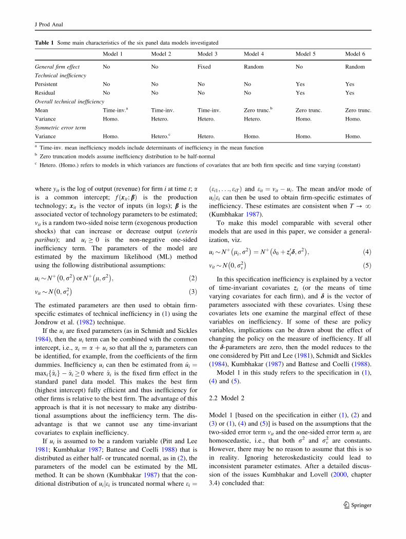
ciency. These six models are briefly summarized in

Table 1.

2.1 Model 1

Here we consider generalization of the first generation

panel data models (Pitt and Lee 1981; Schmidt and Sickles

1984; Kumbhakar 1987; Battese and Coelli 1988), which

are of the form:

yit ¼ aþ f xit; bð Þ þ vit � ui ð1Þ

2 Wang and Ho (2010) generalized the Battese–Coelli formulation in

which the temporal pattern of inefficiency is made firm specific by

specifying it as a function of covariates that can change both

temporally and cross-sectionally.

J Prod Anal

123

where yit is the log of output (revenue) for firm i at time t; ais a common intercept; f xit; bð Þ is the production

technology; xit is the vector of inputs (in logs); b is the

associated vector of technology parameters to be estimated;

vit is a random two-sided noise term (exogenous production

shocks) that can increase or decrease output (ceteris

paribus); and ui C 0 is the non-negative one-sided

inefficiency term. The parameters of the model are

estimated by the maximum likelihood (ML) method

using the following distributional assumptions:

ui�Nþ 0; r2� �

or Nþ l; r2� �

; ð2Þ

vit �N 0; r2v

� �ð3Þ

The estimated parameters are then used to obtain firm-

specific estimates of technical inefficiency in (1) using the

Jondrow et al. (1982) technique.

If the ui are fixed parameters (as in Schmidt and Sickles

1984), then the ui term can be combined with the common

intercept, i.e., ai = a ? ui so that all the ai parameters can

be identified, for example, from the coefficients of the firm

dummies. Inefficiency ui can then be estimated from ui ¼maxifaig � ai� 0 where ai is the fixed firm effect in the

standard panel data model. This makes the best firm

(highest intercept) fully efficient and thus inefficiency for

other firms is relative to the best firm. The advantage of this

approach is that it is not necessary to make any distribu-

tional assumptions about the inefficiency term. The dis-

advantage is that we cannot use any time-invariant

covariates to explain inefficiency.

If ui is assumed to be a random variable (Pitt and Lee

1981; Kumbhakar 1987; Battese and Coelli 1988) that is

distributed as either half- or truncated normal, as in (2), the

parameters of the model can be estimated by the ML

method. It can be shown (Kumbhakar 1987) that the con-

ditional distribution of uijei is truncated normal where ei ¼

ðei1; . . .; eiTÞ and eit ¼ vit � ui. The mean and/or mode of

uijei can then be used to obtain firm-specific estimates of

inefficiency. These estimates are consistent when T ? ?(Kumbhakar 1987).

To make this model comparable with several other

models that are used in this paper, we consider a general-

ization, viz.

ui�Nþ li; r2

� �¼ Nþ d0 þ z0id; r

2� �

; ð4Þ

vit �N 0; r2v

� �ð5Þ

In this specification inefficiency is explained by a vector

of time-invariant covariates zi (or the means of time

varying covariates for each firm), and d is the vector of

parameters associated with these covariates. Using these

covariates lets one examine the marginal effect of these

variables on inefficiency. If some of these are policy

variables, implications can be drawn about the effect of

changing the policy on the measure of inefficiency. If all

the d-parameters are zero, then the model reduces to the

one considered by Pitt and Lee (1981), Schmidt and Sickles

(1984), Kumbhakar (1987) and Battese and Coelli (1988).

Model 1 in this study refers to the specification in (1),

(4) and (5).

2.2 Model 2

Model 1 [based on the specification in either (1), (2) and

(3) or (1), (4) and (5)] is based on the assumptions that the

two-sided error term vit and the one-sided error term ui are

homoscedastic, i.e., that both r2 and rv2 are constants.

However, there may be no reason to assume that this is so

in reality. Ignoring heteroskedasticity could lead to

inconsistent parameter estimates. After a detailed discus-

sion of the issues Kumbhakar and Lovell (2000, chapter

3.4) concluded that:

Table 1 Some main characteristics of the six panel data models investigated

Model 1 Model 2 Model 3 Model 4 Model 5 Model 6

General firm effect No No Fixed Random No Random

Technical inefficiency

Persistent No No No No Yes Yes

Residual No No No No Yes Yes

Overall technical inefficiency

Mean Time-inv.a Time-inv. Time-inv. Zero trunc.b Zero trunc. Zero trunc.

Variance Homo. Hetero. Hetero. Hetero. Homo. Homo.

Symmetric error term

Variance Homo. Hetero.c Hetero. Homo. Homo. Homo.

a Time-inv. mean inefficiency models include determinants of inefficiency in the mean functionb Zero truncation models assume inefficiency distribution to be half-normalc Hetero. (Homo.) refers to models in which variances are functions of covariates that are both firm specific and time varying (constant)

J Prod Anal

123

• Ignoring heteroskedasticity of the symmetric error term

vit gives consistent estimates of the frontier function

parameters (b). Heteroskedasticity refers to models in

which variances are functions of covariates that are

both firm specific and time varying, except that the

intercept (a) is downward biased. Estimates of technical

efficiency will also be biased.

• Ignoring heteroskedasticity of the one-sided technical

inefficiency error component ui causes biased estimates

of both the parameters of the frontier function and the

estimates of technical efficiency.

The other problem in Model 1 is that inefficiency is time

invariant, which is quite restrictive. Model 2 is an exten-

sion of Model 1 that allows for heteroskedasticity in both

the one-sided technical inefficiency error component and in

the symmetric noise term. This model is frequently termed

the doubly heteroskedastic model in the literature. It is

specified as:

yit ¼ aþ f xit; bð Þ þ vit � uit ð6Þ

uit �Nþ l; r2it

� �¼ Nþ l; exp xu0 þ z0u;itxu

� �� �ð7Þ

vit �N 0; r2v;it

� �¼ N 0; exp xv0 þ z0v;itxv

� �� �ð8Þ

Although both the Kumbhakar and the Battese–Coelli mod-

els are based on assumptions that u and v are homoskedastic

[cf. (4) and (5) above], such assumptions are not necessary.

The model in (6)–(8) generalizes the models proposed by

Kumbhakar and by Battese–Coelli by making both u and v

heteroskedastic. In the variance function xu0 is a constant

term, the zu;it vector includes exogenous variables associated

with variability in the technical inefficiency function, and xu

is the corresponding coefficient vector. Similarly, xv0 is the

constant term, the vector zv;it includes exogenous variables

(that can be time varying) associated with variability in the

noise term, and xv is the corresponding coefficient vector.

Parameterizing r2v;it, as done here to model production vari-

ability within a stochastic production function framework, is

an alternative to well-known ‘production risk’ specification

of Just and Pope (1978).

It is also possible to use (6)–(8) and change (7) to

uit �Nþ 0; r2it

� �¼ Nþ 0; exp xu0 þ z0u;itxu

� �� �(see Caudill

and Ford 1993; Caudill et al. 1995; Hadri 1999). Another

option is to consider a further generalization in which both

the mean and variance of u are functions of z variables

(Wang 2002), i.e.,

uit �Nþ lit; r2it

� �¼ Nþ d0 þ z0itd; exp xu0 þ z0u;itxu

� �� �

ð7aÞ

Wang demonstrated that parameterizing both the mean

and variance of the one-sided technical inefficiency error

component allows non-monotonic efficiency effects, which

can be useful for understanding the relationships between

the inefficiency and its exogenous determinants. The

models of Huang and Liu (1994) and Battese and Coelli

(1995), in which variances are assumed to be constant, are

special cases of the Wang (2002) model. Given all these

generalizations, there is no reason for using the Battese–

Coelli model without scrutinizing it carefully, viz., testing

it against more general specifications. In other words, many

alternative specifications are possible.

In the analysis reported below we used the specification

in (6), (7a) and (8) as Model 2, and the parameters of the

model are estimated by ML.

2.3 Model 3

Both Model 1 and various versions of Model 2 account for

the panel data structure by including time as an exogenous

variable in the model components. In Model 3, which is an

extension of the model by Kumbhakar and Wang (2005),

we accommodate the panel nature of the data by intro-

ducing firm-specific intercepts, i.e.,

yit ¼ ai þ f xit; bð Þ þ vit � uit ð9Þuit ¼ Gtui ð10ÞGt ¼ exp ctð Þ ð11Þ

ui�Nþ li; r2i

� �¼ Nþ d0 þ z

0

id; exp xu0 þ z0

u;ixu

� �� �

ð12Þ

vit �N 0; r2v;it

� �¼ N 0; exp xv0 þ z

0

v;itxv

� �� �ð13Þ

The above equations describe Model 3 used in the analysis

below. Compared to Models 1 and 2, Model 3 exploits the

panel structure of the data better, since the intercept term ai

in Eq. (9) controls for unobserved heterogeneity or firm-

specific fixed effects. Note that, in this specification, firm

effects (ai whether fixed or random) are not regarded as

part of inefficiency. In other words, this model can separate

technical inefficiency (time varying) from time-invariant

firm effects simply by assuming (without any explanation)

that firm effects do not include inefficiency.

Note that in specifying inefficiency as uit = Gtui in (10)

we are making the assumption that it can be represented

as a product of Gt, a deterministic function of time, and ui,

a non-negative random variable. This is one way of

exploiting the panel feature of the data without introduc-

ing additive firm effects. Kumbhakar (1991) formulated

Gt ¼ ð1þ expðb1t þ b2t2ÞÞ�1so that Gt can be monoton-

ically increasing (decreasing) or concave (convex)

depending on the signs and magnitudes of b1 and b2.

Battese and Coelli (1992) simplified the formulation by

J Prod Anal

123

assuming Gt ¼ exp �cðt � TÞð Þ. Their specification allows

inefficiency to increase or decrease exponentially

depending on the sign of c. Thus the Kumbhakar (1991)

model is slightly more general because it allows more

flexibility in the temporal behavior of inefficiency. Feng

and Serletis (2009) extended the Battese–Coelli formula-

tion by specifying Gt ¼ exp �c1ðt � TÞ � c2ðt � TÞ2� �

.

Wang and Ho (2010) further generalized the model by

introducing covariates in the G function that are both firm

and time specific. Our Model 3 constitutes (9)–(13). Note

that the parameters and firm effects in this model are

identified through distributional assumptions and ML

estimation.3

2.4 Model 4

Greene (2005a, b) proposed two models, which he called

‘true’ fixed-effects frontier model and ‘true’ random-

effects frontier model. The purpose of these models is to

disentangle firm heterogeneity or firm effects from tech-

nical efficiency. His ‘true’ random effect frontier model,

which we label Model 4, is specified as:

yit ¼ aþ xið Þ þ f xit; bð Þ þ vit � uit ð14Þ

uit �Nþ 0; r2it

� �¼ Nþ 0; exp xu0 þ z

0

u;itxu

� �� �ð15Þ

vit �N 0; r2v

� �ð16Þ

xi�N 0;r2x

� �ð17Þ

The main difference between Models 3 and 4 is the way

inefficiency is modelled. In Kumbhakar and Wang (2005)

inefficiency is first specified as the product of Gt, which is

usually a function of time, and ui. The latter is a truncated

normal variable the mean and variance of which depend on

the vector of firm-specific variables. These variables cannot

be time varying because ui is time invariant. In contrast,

inefficiency in Model 4 is not a product of Gt and ui and

therefore the mean and variance of uit can depend on

variables that are not necessarily time invariant. Naturally

the likelihood functions of these two models are different.

Kumbhakar and Wang (2005) treated ai as fixed while

Greene (2005a, b) allowed to treat it as either random or

fixed. We expect that models that allow time-invariant

effects but do not treat them as inefficiency (as in Model 4)

will give lower estimates of inefficiency. This is likely to

be case irrespective of whether the time-invariants effects

are treated as fixed or random.

Because of its complexity the Greene model is estimated

by the maximum simulated likelihood method. Chen et al.

(2011) proposed estimating the within transformed model

using the standard ML method. This procedure does not

suffer from ‘incidental parameter’ problem when the firm

effects are fixed.

2.5 Model 5

In Model 4 the firm effects are not regarded as part of

inefficiency. This is in contrast to Model 1 in which firm

effects are regarded as inefficiency. Whether firm effects

(fixed or random) are parts of inefficiency or not depends

on how these effects are interpreted. For example, if

management is time invariant, it will be captured by firm

effects. The question is whether it is an input in the pro-

duction process or inefficiency. Hardly any economic

rationale is provided either in favor of or against treating

firm effects as inefficiency.

It might be undesirable to force inefficiency to be time

invariant and Kumbhakar and Heshmati (1995)4 proposed a

model in which technical inefficiency is assumed to have a

persistent firm-specific (time-invariant) component and a

time-varying residual component. Thus, in their model firm

effects are treated as persistent inefficiency. Kumbhakar

and Heshmati argued that identifying the magnitude of

persistent inefficiency may be important, at least in panel

data with a short time span, because it reflects the effects of

inputs such as management that vary between firms but not

over time. Thus, unless there are changes that affect the

management style of individual firms, such as a change in

firm ownership, or changes in the operating environment,

such as a change in government regulations, taxes or sub-

sidies, it is very unlikely that the persistent inefficiency

component will change. On the other hand, the residual

component of inefficiency might change over time. It is

possible to explain the persistent component by making it a

function of covariates that are time invariant (e.g. measures

of a manager’s innate ability and skills). Similarly, the

residual component can be explained by factors such as

experience that might vary over time and across firms. It is

likely that a part of inefficiency is firm effects (effects of

omitted/unobserved time-invariant factors). However, as

argued by Kumbhakar and Heshmati (1995), the distinction

between the persistent and residual components of ineffi-

ciency is important because they have different policy

implications. Thus our Model 5 is the Kumbhakar–Hesh-

mati model that is specified as:

3 Model 3 as well as the ‘true’ fixed-effect frontier models by Greene

(2005a, b) (Model 4 below) include a potential incidental parameters

problem. A recent paper by Chen et al. (2011) addressed this problem.

Wang and Ho (2010) proposed an alternative estimation model that is

immune to the incidental parameters problem. A fixed-effect panel

stochastic frontier model is estimated by applying first-difference and/

or within transformation methods.

4 Similar models to that of Kumbhakar and Heshmati (1995) were

reported by Kumbhakar and Hjalmarsson (1993, 1995).

J Prod Anal

123

yit ¼ a0 þ f xit; bð Þ þ vit � gi � uit ð18Þ

where vit is noise; gi C 0 represents persistent technical

inefficiency; uit C 0 represent time-varying inefficiency;

and gi ? uit is overall technical inefficiency. The error

components are assumed to be independent of each other

and also independent of xit. For estimation purposes we

rewrite (18) as

yit ¼ a�0 þ f xit; bð Þ þ vit � u�it � g�i ð19Þ

where a�0 ¼ a0 � E gið Þ � E uitð Þ; u�it ¼ uit � E uitð Þ; and

g�i ¼ gi � E gið Þ.The model can be estimated in three steps. In step 1 we

estimate Eq. (19) via a standard random effect regression

model for panel data. This gives consistent estimates of b.

We also get predicted values of g�i and u�it as a by-product

of using a random effects panel model. The estimates of g�iprovide the best linear predictor of random individual

effects. Note that in step 1 we are using a pure random

effects panel model.

In step 2, the persistent technical efficiency is estimated,

using the predicted values of g�i . If we denoted these by g�i ,

persistent technical inefficiency can then be estimated from

gi ¼ Max g�i� �

� g�i ð20Þ

Finally, the persistent technical efficiency measure (PTE) is

obtained from expð�giÞ.In step 3 the residual technical efficiency is estimated.

For this we go back to step 1 and obtain the residuals (i.e.,

yit � f xit; bð Þ þ gi ¼ a0 þ vit � uit). By assuming that vit is

iid N 0; r2v

� �, and uit is iid Nþ 0; r2ð Þ, we can simply

maximize the log-likelihood function for the following

standard normal-half normal SF model for pooled data

rit ¼ a0 þ vit � uit ð21Þ

where rit ¼ yit � f xit; bð Þ þ gi: In practice we use the

estimated values of b and gi to define rit. That is, sampling

variability associated with b and gi is ignored. Using the

standard frontier model on (21) we get estimates of a0, r2v

and r2. The Jondrow et al. (1982) result can then be used to

estimate residual technical inefficiency, uit, conditional on

the estimated residuals, vit � uitð Þ. We can use these uit to

calculate time-varying residual technical inefficiency

defined as RTE ¼ exp �uitð Þ, and then find overall technical

efficiency defined as the product of PTE and RTE, i.e.,

OTE ¼ PTE � RTE.

2.6 Model 6

Unlike Model 4, Model 5 does not take into account any

fixed or random effects associated with unobserved factors

that are not related to inefficiency. Model 6 is a version of

Model 5, modified and extended to include random firm

effects. The presence of such effects can be justified, for

example, by making an argument that there are unobserved

time-invariants inputs that are not inefficiency. In agricul-

ture one such might be land quality. Our Model 65 is

specified as:

yit ¼ a0 þ f xit; bð Þ þ li þ vit � gi � uit ð22Þ

where li are random firm effects that capture unobserved

time-invariant inputs. This model has four components two

of which (gi and uit) are inefficiency and the other two are

firm effects and noise (li and vit). These components

appeared in other models in various combinations but not

all at the same time in one model. This new model fills

several gaps in the panel SF literature currently used. First,

although some of the time-varying inefficiency models

presently used in the literature can accommodate firm

effects, these models fail to take into account the possible

presence of some factors that might have permanent (i.e.,

time-invariant) effects on firms’ inefficiency. Here we call

them permanent/time-invariant components of inefficiency.

Second, SF models allowing time-varying inefficiency

assume that a firm’s inefficiency at time t is independent of

its previous level inefficiency. It is more sensible to assume

that a firm may eliminate part of its inefficiency by

removing some of the short-run rigidities, while some other

sources of inefficiency might stay with the firm over time.

The latter is captured by the time-varying component uit.

Finally, many panel SF models do consider permanent/

time-invariant inefficiency effects but do not take into

account the effect of unobserved firm heterogeneity on

output. By doing so, these models confound permanent/

time-invariant inefficiency with firm effects (heterogene-

ity). Models proposed by Greene (2005a, b), Kumbhakar

and Wang (2005), Wang and Ho (2010) and Chen et al.

(2011) decompose the error term in the production function

into three components: a producer-specific time-varying

inefficiency term; a producer-specific random- or fixed-

effects capturing latent heterogeneity; and a producer- and

time-specific random error term. However, these models

consider any producer-specific, time-invariant component

as unobserved heterogeneity. Thus, although firm hetero-

geneity is now accounted for, it comes at the cost of

ignoring long-term (persistent) inefficiency. In other words,

long-run inefficiency is again confounded with latent

heterogeneity.

Estimation of the model can be done in a single stage

ML method based on distributional assumptions on the four

components (Colombi et al. 2011). Here we consider a

5 For a fuller treatment of this model estimated by ML method

(which is quite involved) see Colombi et al. (2011). Here we consider

a multi-step approach which is much simpler to use.

J Prod Anal

123

simpler multi-step procedure. For this, we rewrite the

model in (22) as

yit ¼ a�0 þ f xit; bð Þ þ ai þ eit ð23Þ

where a�0 ¼ a0 � E gið Þ � E uitð Þ; ai ¼ li � gi þ E gið Þ; and

eit ¼ mit � uit þ E uitð Þ. With this specification ai and eit

have zero mean and constant variance. This model can be

estimated in three steps. Since Eq. (23) is the familiar panel

data model, in step 1 the standard random effect panel

regression is used to estimate b. This procedure also gives

predicted values of ai and eit, which we denote by ai and eit.

In step 2, the time-varying technical inefficiency, uit, is

estimated. For this we use the predicted values of eit from

step 1. Since

eit ¼ mit � uit þ E uitð Þ ð24Þ

by assuming vit is iid N 0;r2v

� �, and uit is iid Nþ 0; r2ð Þ

(which means E uitð Þ ¼ffiffiffiffiffiffiffiffi2=p

pr) and ignoring the differ-

ence between the true and predicted values of eit (which is

the standard practice in any two- or multi-step procedure),

we can estimate Eq. (24) using the standard SF technique.

This procedure gives prediction of the time-varying resid-

ual technical inefficiency components, uit (the Jondrow

et al. 1982 estimator) which can be used to estimate

residual technical efficiency, RTE ¼ expð�uitÞ.In step 3 we can estimate gi following a similar proce-

dure as in step 2. For this we use the best linear predictor of

ai from step 1. Since

ai ¼ li � gi þ E gið Þ ð25Þ

by assuming li is iid N 0; r2l

� �, gi is iid Nþ 0; r2

g

� �(which

in turn means E gið Þ ¼ffiffiffiffiffiffiffiffi2=p

prg) we can estimate Eq. (25)

using the standard normal-half normal SF model cross-

sectionally and obtain estimates of the persistent technical

inefficiency components, gi, using the Jondrow et al.

(1982) procedure. Persistent technical inefficiency can then

be estimated from PTE ¼ expð�giÞ, where gi is the Jond-

row et al. (1982) estimator of gi: The overall technical

efficiency (OTE) is then obtained from the product of PTE

and RTE, i.e., OTE ¼ PTE � RTE.

It is possible to extend Models 6 (in steps 2 and 3) to

include non-zero mean of persistent and time-varying

inefficiency and also to account for heteroskedasticity in

either or both. These extensions are left for the future.

Also, the finite sample behaviour of estimators of persistent

and residual inefficiency is left for the future.

3 Data

The data source is the Norwegian Farm Accountancy

Survey. This is an unbalanced set of farm-level panel data,

collected by the Norwegian Agricultural Economics

Research Institute (NILF). It includes farm production and

economic data collected annually from about 1,000 farms,

divided between different regions, farm size classes, and

types of farms. Participation in the survey is voluntary.

There is no limit on the numbers of years a farm may be

included in the survey. Approximately 10 % of the survey

farms are replaced per year. The farms are classified

according to their main category of farming, defined in

terms of the standard gross margins of the farm enterprises.

Thus, a farm is categorized as a grain farm if more than

50 % of the total standard gross margin is from grain

production.

The data set used in the analysis is an unbalanced

panel with 687 observations on 154 grain farms from

2004 to 2008. We included only farms in the lowlands of

Eastern Norway, Jæren, and Mid-Norway. Within each of

these three regions the growing conditions are reasonably

similar, and these are the main grain producing regions

of Norway. To accommodate panel features in estima-

tion, only those farms for which at least 2 years of data

were available were included in the analysis. The aver-

age duration of farms in the survey for the sample used

is about 3 years. This relatively short average duration

will affect our results because estimates of firm-specific

parameters are consistent only as T approaches infinity.

Although the usual caveats of SF modeling apply about

the consistency of estimates of inefficiency, our main

objectives of demonstrating and comparing models

with firm effects and time-invariant inefficiency are

not compromised by the short duraton of farms in the

data.

Grain farms usually produce several types of grains

(wheat, barley, oats etc.), and, by the classification sys-

tem applied, have few (if any) farm activities besides

grains. The total output, y1, is aggregated and measured

as the farm revenue (exclusive of coupled and environ-

mental subsidies) in Norwegian kroner (2008 NOK)

per year, obtained by deflating the annual farm revenues

to 2008 revenues using the consumer price index

(CPI).

The production function f xit; bð Þ in Models 1 and 6 is

specified with the following input variables: x1 is labor

hours used on the farm, measured as total number of hours

worked, including management, family and hired workers;

x2 is productive farmland in hectares; x3 is variable farm

inputs, measured by variable costs, deflated by the CPI to

2008 NOK prices; x4 is farm fixed and capital costs, also

deflated by the CPI to 2008 NOK prices; and tð1; . . .; 5Þ is a

time trend. The fixed and capital costs include incurred

expenditure on fixed costs items plus depreciation and

required return on farm capital tied up in machinery,

buildings and livestock.

J Prod Anal

123

The z-variables in this study consist of the following:6 z1

is income share from off-farm work, measured as the

farmer’s net income off the farm as a proportion of the

farmer’s total net income on and off the farm within a year;

z2 is share of income from coupled (output related) subsi-

dies, measured as coupled subsidies received as a propor-

tion of the total farm net income within a year; z3 is

environmental payments share, measured as the farm

environmental payments received as a proportion of the

total farm net income within a year; z4 is entrepreneurial

orientation index;7 z5 is experience, measured as number of

years as a farmer; z6 is a dummy variable of one if the

farmer has only primary education (i.e. no secondary or

higher education); and z7 is a dummy variable of one if the

farmer has secondary education (i.e. high school, but no

higher education). Descriptive statistics of the variables

used in the study are reported in Table 2.

We choose a translog specification of the f xit; bð Þfunction in our empirical analysis in Models 1–6 because

of its flexibility (Christensen et al. 1973).

We used log values for the input variables in the tran-

slog production function. Prior to taking logs the x-vari-

ables were scaled (divided by their geometric means).

Consequently, the first-order coefficients in the model can

Table 2 Descriptive statistic (N = 687)

Variable Label Mean SD Min Max

Production function variables

y1 Farm revenue (2008 NOK) 1,085,411 948,950 80,610 9,386,916

x1 Labor (hours) 2,579 1,480 74 15,200

x2 Farmland (hectare) 35.3 19.5 0.5 129.4

x3 Variable farm inputs (2008 NOK) 480,793 509,090 21,397 3,383,073

x4 Fixed farm input and capital costs (2008 NOK) 415,583 262,028 40,238 2,231,058

t Year (1 = 2004, 5 = 2008) 3.1 1.4 2 5

Inefficiency determinant variables and heteroskedasticity variables in the inefficiency function

z1 and zu1 Farm-specific off-farm income share 0.57 0.23 0.08 0.94

z2 and zu2 Farm-specific coupled subsidy income share 0.20 0.09 0.01 0.41

z3 and zu3 Farm-specific environmental subsidy income share 0.04 0.03 0 0.16

z4 and zu4 Entrepreneurial orientation index 2.85 1.19 1 5.58

z5 and zu5 Farmer experience, years 18.98 9.41 2 39

z6 and zu6 Primary education, dummy 0.29 0.42 0 1

z7 and zu7 Secondary education, dummy 0.45 0.50 0 1

Heteroskedasticity in error component variables

zv1 Off-farm income share 0.57 0.25 0 1.75

zv2 Coupled subsidy income share 0.20 0.10 0 0.67

zv3 Environmental subsidy income share 0.04 0.04 0 0.25

zv4 Entrepreneurial orientation index 2.85 1.19 1 5.58

zv5 Farmer experience, years 18.98 9.41 2 39

zv6 Primary education, dummy 0.29 0.42 0 1

zv7 Secondary education, dummy 0.45 0.50 0 1

6 Two modeling approaches have mainly been used to analyze effects

of subsidies on farm performance. The first approach treats subsidies

as traditional inputs (such as land, labour and capital) in the production

function to allow for a direct influence on productivity. This approach

suffers from certain problems: (1) while traditional inputs are

necessary for production, subsidies are not; and (2) subsidies alone

cannot produce any output, while traditional inputs can. The second

approach employs a stochastic production function approach and only

allows subsidies to affect productivity through the technical ineffi-

ciency function. This latter approach, as is used in this study, escapes

traditional-input criticism, but it does not simultaneously examine the

impact of subsides on productivity and efficiency changes. For a more

thorough discussion of these traditional and some recent more

advanced approaches, see for example McCloud and Kumbhakar

(2008) and Kumbhakar and Lien (2010).

7 A farmer survey was done in 2009 to obtain attitudinal and

behavioral data to supplement the panel of farm accountancy survey

data. One sub-set of questions, called entrepreneurial orientation (EO)

by Wiklund (1998), comprised eight questions about innovativeness,

risk taking and proactiveness. The farmers were asked to respond on a

Likert-scale from 1 to 7. Our single measure of EO was derived from

these responses through a second-order factor analysis. Collapsing

responses into one measure is consistent with most of the earlier EO

studies in the literature (Rauch et al. 2009).

J Prod Anal

123

02

46

Pro

port

ion(

farm

s)

.2 .3 .4 .5 .6 .7 .8 .9 1

Technical efficiency

Model 1

01

23

45

Pro

port

ion(

farm

s)

.2 .3 .4 .5 .6 .7 .8 .9 1

Technical efficiency

Model 2

01

23

Pro

port

ion(

farm

s)

.2 .3 .4 .5 .6 .7 .8 .9 1

Technical efficiency

Model 3

05

1015

Pro

port

ion(

farm

s)

.2 .3 .4 .5 .6 .7 .8 .9 1

Technical efficiency

Model 4

01

23

45

Pro

port

ion(

farm

s)

.2 .3 .4 .5 .6 .7 .8 .9 1

Overall technical efficiency

Model 5

02

46

Pro

port

ion(

farm

s)

.2 .3 .4 .5 .6 .7 .8 .9 1

Overall technical efficiency

Model 6

Fig. 1 Technical efficiency distributions of sample farms for Models 1–6

.5.6

.7.8

.91

Tec

hnic

al e

ffici

ency

2004 2005 2006 2007 2008

Year

Model 1

.5.6

.7.8

.91

Tec

hnic

al e

ffici

ency

2004 2005 2006 2007 2008

Year

Model 2

.5.6

.7.8

.91

Tec

hnic

al e

ffici

ency

2004 2005 2006 2007 2008

Year

Model 3

.5.6

.7.8

.91

Ove

rall

tech

nica

l effi

cien

cy

2004 2005 2006 2007 2008

Year

Model 4

.5.6

.7.8

.91

Ove

rall

tech

nica

l effi

cien

cy

2004 2005 2006 2007 2008

Year

Model 5

.5.6

.7.8

.91

Ove

rall

tech

nica

l effi

cien

cy

2004 2005 2006 2007 2008

Year

Model 6

Fig. 2 The mean, first and third quartile values (middle, bottom and top lines) of technical efficiency of sample farms for Models 1–6

J Prod Anal

123

be interpreted as elasticities of output evaluated at the

means of the data.

4 Results and interpretations

4.1 Technical efficiency

Figure 1 presents the kernel density distribution of the

technical efficiency estimates for Models 1–6 (overall tech-

nical efficiency for Models 5 and 6), and Fig. 2 shows the

mean, first quartiles and third quartiles scores per year for the

same models. The various models clearly produce different

empirical distributions, in some instances markedly so.

The mean technical efficiency of Model 4 (0.91) is the

highest, while it is smallest (0.64) for Model 5. The spread

of the efficiency scores per model can be seen from Fig. 2,

where spread is illustrated by the inter-quartile ranges.

Model 2 has the widest spread of efficiency scores, slightly

wider than Model 3, while Model 4 has an appreciably

narrower spread than the other models. The figures show

that, despite the difference in spreads, the time-series pat-

terns for the different models are quite similar.

The mean efficiency values in Models 1 and 2 (which

allow both u and v to be heteroskedastic) are almost the

same. However, the maximum and especially the minimum

efficiency scores are more extreme when allowance is

made for heteroskedasticity.

In Model 3, the combined effect of accounting for heter-

oskedasticity and firm-specific random effects resulted in a

reduction in mean technical efficiency (to 0.73), with a spread

about the same as for Model 2. These results are largely

consistent with earlier empirical findings. Hadri et al. (2003a,

b), in their studies of cereal farms in UK, found that cor-

recting for heteroskedasticity had a significant effect on the

spread of the measure of technical efficiency. Caudill et al.

(1995) found a dramatic decrease in the technical efficiency

measures from inclusion of heteroskedasticity in their study

of bank cost data. It appears that inclusion of a random effect

(in Model 3, compared to Model 2) has also contributed to

reduced estimates of technical efficiency. Yet such an effect

seems counter-intuitive, since the random effect component

should pick up some of the technical efficiency effect found

in models without a random effect. Evidently, it is hard to

form firm conclusions about the interaction between the firm-

specific random effect, the mean efficiency function, the

heteroskedasticity in the efficiency function and the heter-

oskedasticity in the symmetric error component.

Instead of focusing on heteroskedasticity, Models 4, 5

and 6 provide ways to account for heterogeneity between

firms and to specify and eventually decompose the tech-

nical efficiency component. The results of decomposition

of technical efficiency into persistent technical efficiency

and time-varying technical efficiency for Models 5 and 6

are plotted in Fig. 3.

One problem with Model 5 is that all time-invariant noise

is measured as persistent technical inefficiency. It seems

plausible that the persistent technical inefficiency part in

Model 5 is the main reason for the low overall technical

efficiency estimates. In other words, some potential firm

effects may have been captured in the inefficiency mea-

sures, as the distributions in the upper part of Fig. 3 appear

to confirm. The mean persistent technical efficiency score in

Model 5 is 0.71 while the mean residual technical efficiency

score is 0.89. As shown in the lower part of Fig. 3 for Model

6, the spread of efficiency is significantly higher for the

persistent component than for the residual component.

These results suggest that persistent technical inefficiency is

a larger problem than residual technical inefficiency in

Norwegian grain farming. Kumbhakar and Heshmati (1995)

also found more persistent technical efficiency than residual

technical efficiency in their analysis of dairy farms in

Sweden for the period 1976–1988. A high degree of per-

sistent technical efficiency could reflect long-run problems.

There has been a high level of government support in

Norwegian agriculture for many decades that may have

caused some persistent inefficiency. If there is a wish to

reduce the governmental support level, and still keep the

living standard in the long run, focus should be on measures

to reduce persistent technical inefficiency. For example, it

may help to consider measures that encourage long-term

structural adjustment toward fewer larger farms or switches

to other more productive farm activities.

In Model 4, the ‘true’ random effects frontier model, the

firm effects are not considered to be inefficiency, leading to

high efficiency scores (Fig. 1) and low dispersion (Fig. 2).

Greene (2005a, b) also found in a study of the US banking

industry that the ‘true’ random effects results had higher

and less dispersed technical efficiency scores than results

for other models considered.

Neither the assumption that all time-persistent noise is

inefficiency (Model 5) nor that no firm-specific effects are

inefficiency (Model 4) might be true. Model 6 overcomes

these problems by decomposing the time-persistent noise

into a firm effect and a persistent technical inefficiency

effect. The results are efficiency scores between the scores

for Models 4 and 5 (Fig. 1). The mean overall efficiency

score for Model 6 is 0.78, and the score spread is between

that of Model 4 (low spread) and Model 5 (high spread;

Fig. 2). Compared to Model 5, Model 6 has a higher per-

sistent technical efficiency score (0.87) with a less dis-

persed distribution (Fig. 3).

As the above results illustrate, the efficiency scores are,

as expected, sensitive to model specification. How then are

the technical efficiency ranking of farms affected by dif-

ferent model specifications used? In Table 3 pairwise rank-

J Prod Anal

123

order correlations for Models 1–6 (overall technical effi-

ciency for Models 5 and 6) illustrate the differences

between the models in technical efficiency ranking of the

sample farms. In Fig. 4 scatter plot matrices for Models

1–6 graphically illustrate the differences between the

models in the ranking of the farms in the sample by tech-

nical efficiency estimates. A perfect match between two

models would show up as a straight line in the graph, and

not as a scatter of points.

The patterns of results between Models 1 and 2 and

between Models 5 and 6 seem to be the most consistent, i.e.,

these model comparisons have the least dispersed scatter

plots, strongest congruence, and most consistent rankings.

The correlations in Table 3 confirm this observation. The

scatter plot between Models 1 and 2 seems quite linear,

indicating that the efficiency score are rather consistent for

these models. However, the plot between Models 6 and 5

indicates a systematically lower efficiency score in the high

score group, resulting in the non-linear pattern shown. Both

Models 1 and 6 have quite similar technical efficiency

assessments to those for Model 4. On the other hand, the

results for Models 2 and 3 are quite different and these two

models also show quite inconsistent patterns and rankings

of results relative to the other models investigated.

Table 4 shows that the Kendall’s rank-order correlation

for persistent technical efficiency measure between Models

5 and 6 are 1, i.e. perfect rank-order correlation. Further,

the efficiency assessments of residual technical efficiency

for these two models are perfectly positively correlated,

while the results based on persistent and residual technical

efficiency are to a large extent independent or random, with

a rank-order correlation of 0.14.

01

23

4

Pro

port

ion(

farm

s)

.2 .3 .4 .5 .6 .7 .8 .9 1

Persistent technical efficiency

Model 5

05

1015

Pro

port

ion(

farm

s)

.2 .3 .4 .5 .6 .7 .8 .9 1

Residual technical efficiency

Model 5

02

46

8

Pro

port

ion(

farm

s)

.2 .3 .4 .5 .6 .7 .8 .9 1

Persistent technical efficiency

Model 6

05

1015

Pro

port

ion(

farm

s)

.2 .3 .4 .5 .6 .7 .8 .9 1

Residual technical efficiency

Model 6

Fig. 3 Distributions of persistent technical efficiency (to left) and residual technical efficiency (to right) distributions for Models 5 and 6

Table 3 Kendall’s rank-order

correlation between of technical

efficiency estimates for Models

1 to 6. For Models 5 and 6

overall technical efficiency

(OTE) is calculated

Model 1 Model 2 Model 3 Model 4 Model 5 OTE

Model 2 0.79

Model 3 0.73 0.69

Model 4 0.73 0.59 0.58

Model 5 OTE 0.52 0.38 0.49 0.68

Model 6 OTE 0.54 0.38 0.45 0.73 0.88

J Prod Anal

123

4.2 Elasticities, returns to scale, technical change

and efficiency/variance determinants

For all models the estimated output elasticities with respect

to labor, land, variable farm inputs and fixed farm input/

capital all differed from zero at the 1 % significance level

(5 % significance level for fixed farm input/capital in

Model 3). The elasticities for labor, land and variable farm

inputs were larger than 0.23 for all models. Estimates of

technological change were statistically significant and

positive for all models at 1.7–2.7 % per year (Table 5 in

the ‘‘Appendix’’).

The yearly mean, first and third quartile values of

returns to scale results for the sample observations are

graphed in Fig. 5. The scale elasticity was highest for

Models 5 and 6 (at 1.21 on average) and lowest for Model

2 (1.04 on average) and Model 4 (1.08 on average). The

estimated scale elasticity was not significantly different

from 1 (at 10 % level) only for Model 2. All models

showed a weak decreasing time trend in scale elasticity,

and the spreads of elasticity estimates were highest for

Models 3, 5 and 6.

Models 1–3 include an inefficiency function and in

Figs. 6 and 7 we have plotted the determinants of effi-

ciency scores against off-farm income share, entrepre-

neurial orientation, coupled subsides income share and

environmental subsidy income. In the lower part of Table 5

(in the ‘‘Appendix’’), the determinants of efficiency scores

and variance parameters are examined at the means of the

variables.

From Fig. 6 we can see that off-farm income share

tended to affect technical efficiency in a negative way, but

with the effect being highly variable between farms. This

negative effect appears to be weaker for Model 3 than for

Models 1 and 2. In other words, the plots for Models 1 and

2 indicate that off-farm income has a weaker negative

effect on farm efficiency than is indicated by the plot for

Model 3. This result supports some earlier studies (e.g.,

Brummer 2001; Goodwin and Mishra 2004) but is at

Model1

Model2

Model3

Model4

Model5 OTE

Model6 OTE

0 .5 1

0

.5

1

0 .5 1

.4

.6

.8

1

.4 .6 .8 1

.4

.6

.8

1

.4 .6 .8 1

0

.5

1

0 .5 1

0

.5

1

Fig. 4 Scatter plot matrices of pairwise technical efficiency estimates for Models 1–6. For Models 5 and 6 overall technical efficiency (OTE) is

plotted. Technical efficiency levels for each scatter plot are shown on both the horizontal and vertical axes for each pair-wise comparison

Table 4 Kendall’s rank-order correlation between Models 5 and 6

for persistent technical efficiency (PTE) and residual technical effi-

ciency (RTE) estimates

Model 5 PTE Model 5 RTE Model 6 PTE

Model 5 RTE 0.14

Model 6 PTE 1.00 0.14

Model 6 RTE 0.14 1.00 0.14

J Prod Anal

123

.95

1.05

1.15

1.25

Ret

urns

to s

cale

2004 2005 2006 2007 2008

Year

Model 1

.95

1.05

1.15

1.25

Ret

urns

to s

cale

2004 2005 2006 2007 2008

Year

Model 2

.95

1.05

1.15

1.25

Ret

urns

to s

cale

2004 2005 2006 2007 2008

Year

Model 3

.95

1.05

1.15

1.25

Ret

urns

to s

cale

2004 2005 2006 2007 2008

Year

Model 4

.95

1.05

1.15

1.25

Ret

urns

to s

cale

2004 2005 2006 2007 2008

Year

Model 5

.95

1.05

1.15

1.25

Ret

urns

to s

cale

2004 2005 2006 2007 2008

Year

Model 6

Fig. 5 The mean, first and third quartile values (middle, bottom and top lines) of the distribution of returns to scale for the sample observations in

Models 1–6

.2.4

.6.8

1

Tec

hnic

al e

ffici

ency

0 .2 .4 .6 .8 1

Off-farm income share

Model 1

.2.4

.6.8

1

Tec

hnic

al e

ffici

ency

0 .2 .4 .6 .8 1

Off-farm income share

Model 2.2

.4.6

.81

Tec

hnic

al e

ffici

ency

0 .2 .4 .6 .8 1

Off-farm income share

Model 3

.2.4

.6.8

1

Tec

hnic

al e

ffici

ency

1 2 3 4 5 6

Ent. orient.

Model 1

.2.4

.6.8

1

Tec

hnic

al e

ffici

ency

1 2 3 4 5 6

Ent. orient.

Model 2

.2.4

.6.8

1

Tec

hnic

al e

ffici

ency

1 2 3 4 5 6

Ent. orient.

Model 3

Fig. 6 Plots of off-farm income share (upper panel) and entrepreneurial orientation (lower panel) versa technical efficiency for the sample farms

J Prod Anal

123

variance with the some other earlier work (e.g., Chavas

et al. 2005; Lien et al. 2010). The study by Lien et al. used

partly the same data as in this study, but estimated an

equation system in which off-farm work was measured by

hours worked off the farm (and not as off-farm income

share), and defined output as quantities (not in monetary

values). The changed specification of the variable, some-

what surprisingly, led to a different finding, suggesting a

need for further investigation.

As far as we know, entrepreneurial orientation has not

been used as an inefficiency determinant in earlier effi-

ciency studies in the agricultural economics literature.

Hence we have no other results to compare with. The lower

part of Fig. 6 shows a weak negative impact of farmers’

entrepreneurial orientation on technical efficiency, albeit

with wide dispersion. We might expect that an innovative

and entrepreneurial attitude would increase the efficiency,

but on the other hand, frequent innovation may also reduce

the efficiency. The combined impact of these two effects

may explain the lack of any clear results.

The coupled subsidy income share (quite clearly), and

environmental subsidy income share (to some extent) seem

to have negative influences on technical efficiency (Fig. 7).

These results support the findings by, for example, Gian-

nakas et al. (2001) and Karagiannis and Sarris (2005).

However, our findings contrast with the study by Kum-

bhakar and Lien (2010). The negative impact of subsidies

may occur because the extra income reduces the motivation

of the farmers to work efficiently.

Wilson et al. (2001) found that managers with more

experience are likely to be more efficient than those with

fewer years of experience, consistent with our Model 2

results but in contrasts with our failure in Models 1 and 3 to

find any significant difference in technical efficiency

between inexperienced and experienced farmers (Table 5

in the ‘‘Appendix’’). Also, education was not a significant

determinant of efficiency in our study.

In addition to the expectation that modeling heteroske-

dasticity should give more reliable production function and

efficiency score estimates, the signs and levels of the

explanatory variables for heteroskedasticity in the one-

sided pre-truncated inefficiency function and in the two-

sided error component could convey important informa-

tion. An examination of the parameters for these variables

in Table 5 (in the ‘‘Appendix’’) shows several inconsistent

results between the models investigated. For example,

while Model 2 shows that off-farm income share signifi-

cantly reduces the variance in technical efficiency, Model 4

shows the opposite. Similarly, Model 3 shows that entre-

preneurial orientation significantly reduces variance in

.2.4

.6.8

1

Tec

hnic

al e

ffici

ency

0 .1 .2 .3 .4

Coupled subsidies

Model 1

.2.4

.6.8

1

Tec

hnic

al e

ffici

ency

0 .1 .2 .3 .4

Coupled subsidies

Model 2.2

.4.6

.81

Tec

hnic

al e

ffici

ency

0 .1 .2 .3 .4

Coupled subsidies

Model 3

.2.4

.6.8

1

Tec

hnic

al e

ffici

ency

0 .05 .1 .15

Env. subsidies

Model 1

.2.4

.6.8

1

Tec

hnic

al e

ffici

ency

0 .05 .1 .15

Env. subsidies

Model 2

.2.4

.6.8

1

Tec

hnic

al e

ffici

ency

0 .05 .1 .15

Env. subsidies

Model 3

Fig. 7 Plot of coupled subsidy income share (upper panel) and environmental subsidy income share (lower panel) versa technical efficiency for

the sample farms

J Prod Anal

123

technical efficiency level, while Models 2 and 4 show the

opposite.

For all models, experience significantly reduces vari-

ability in technical efficiency and reduces the variability in

output. Increasing off-farm income share and entrepre-

neurial orientation among the farmers both contribute to

increased variability in output. But as already mentioned,

these results are model sensitive, and should be interpreted

with care.

5 Concluding comments

Panel data frontier model estimation has been widely

used to estimate technical efficiency. Yet the technical

efficiency measures may be distorted by specification

error. Our concern was not to rank the different models

by some criterion of suitability of statistical reliability.

Rather we sought to demonstrate the range of models

available and differences between them in the assessment

of efficiency.

We showed that allowing for heteroskedasticity in the

error terms can lead to appreciably different technical

efficiency estimates and can also change the ranking of

farms based on efficiency scores. Further, it may not be

valid to assume either that all time-persistent noise is

inefficiency, or that no firm-specific effects are ineffi-

ciency. Our results suggest that models structured to cap-

ture inefficiency that is time invariant (and mixed with firm

effects) may lead to very low efficiency estimates, while

models in which firm effects are not considered to be part

of inefficiency may give high efficiency scores. It seems

that the ‘true’ measure of efficiency may be somewhere

between these extremes and we have presented a new

model which might be said to come closer to capturing this

‘true’ efficiency. This new model also decomposes the

overall technical inefficiency into a persistent component

and a residual component. For the Norwegian grain farms

included in the study, the persistent component of ineffi-

ciency was much larger than the residual inefficiency

component, implying that policy measures that could

reduce persistent inefficiency should be prioritized. Unless

persistent inefficiency is reduced, farmers might not be able

to survive in the long run, especially if competitors are

more efficient.

The variability of the results from the different models

clearly demonstrates the difficulty in ‘correctly’ measuring

efficiencies. No model can be held to be ‘correct’, and the

efficiencies will always be a kind of unobserved or mod-

eled effect. For the future, model choice in empirical

research should not be based on ‘standard practice’, but on

a reasoned choice. A good understanding of the institu-

tional and production environments of the industry under

study, and of the data applied, are crucial in deciding which

estimator should be utilized.

Acknowledgments The authors thank an anonymous referee for

valuable comments and suggestions on an earlier version of this

paper. The authors also acknowledge the financial assistance of the

Research Council of Norway.

Appendix

See Table 5.

Table 5 Estimates of the parameters in the translog frontier production function

Para. Label Model 1 Model 2 Model 3 Model 4 Models 5 and 6

Estimate SE Estimate SE Estimate SE Estimate SE Estimate SE

Elasticities

b1 x1 (Labor) 0.287 (0.036) 0.286 (0.035) 0.305 (0.039) 0.291 (0.025) 0.317 (0.044)

b2 x2 (Farmland) 0.249 (0.037) 0.231 (0.036) 0.336 (0.036) 0.278 (0.022) 0.306 (0.047)

b3 x31 (Variable farm inputs) 0.401 (0.030) 0.371 (0.028) 0.401 (0.027) 0.439 (0.018) 0.533 (0.034)

b4 x41 (Fixed farm inp./capital) 0.200 (0.056) 0.180 (0.052) 0.114 (0.049) 0.123 (0.042) 0.117 (0.063)

Exogenous inefficiency determinantsa

d1 Off-farm work income share 0.710 (0.178) 1.256 (0.227) 0.097 (0.086)

d2 Coupled subsidies income

share

4.262 (0.732) 1.932 (0.348) 2.321 (0.321)

d3 Environmental subsides inc.

share

1.819 (0.766) 2.192 (1.008) -0.603 (0.795)

d4 Entrepreneurial orientation 0.070 (0.025) -0.040 (0.025) 0.030 (0.013)

d5 Experience 0.000 (0.002) 0.009 (0.004) 0.002 (0.002)

d6 Primary education 0.025 (0.061) 0.080 (0.055) 0.086 (0.035)

d7 Secondary education 0.053 (0.049) 0.076 (0.048) 0.069 (0.035)

J Prod Anal

123

References

Aigner DJ, Lovell CAK, Schmidt P (1977) Formulation and

estimation of stochastic frontier production function models.

J Econ 6:21–37

Battese GE, Coelli TJ (1988) Prediction of firm-level technical

efficiencies with a generalized frontier production function and

panel data. J Econ 38:387–399

Battese GE, Coelli TJ (1992) Frontier production functions, technical

efficiency and panel data: with application to paddy farmers in

India. J Prod Anal 3:153–169

Battese GE, Coelli TJ (1995) A model for technical inefficiency

effects in a stochastic frontier production function for panel data.

Empir Econ 20:325–332

Brummer B (2001) Estimating confidence intervals for technical

efficiency: the case of private farms in Slovenia. Eur Rev Agric

Econ 28:285–306

Caudill SB, Ford JM (1993) Biases in frontier estimation due to

heteroskedasticity. Econ Lett 41:17–20

Caudill SB, Ford JM, Gropper DM (1995) Frontier estimation and

firm-specific inefficiency measures in the presence of heteroske-

dasticity. J Bus Econ Stat 13:105–111

Chavas JP, Petrie R, Roth M (2005) Farm household production

efficiency: evidence from the Gambia. Am J Agric Econ

87:160–179

Chen Y-Y, Schmidt P, Wang H-J (2011) Consistent estimation of the

fixed effects stochastic frontier model. Paper presented at the

EWEPA, Verona

Christensen L, Jorgenson D, Lau L (1973) Transcendental logarithmic

production frontiers. Rev Econ Stat 55:28–45

Coelli TJ, Rao DSP, O’Donnell CJ, Battese GE (2005) An Introduc-

tion to efficiency and productivity analysis, 2nd edn. Springer,

New York

Colombi R, Martini G, Vittadini G (2011) A stochastic frontier model

with short-run and long-run inefficiency random effects. Depart-

ment of Economics and Technology Management, Universita di

Bergamo, Italy

Feng G, Serletis A (2009) Efficiency and productivity of the US banking

industry, 1998–2005: evidence from fourier cost functions satis-

fying global regularity conditions. J Appl Econ 24:105–138

Giannakas K, Schoney R, Tzouvelekas V (2001) Technical efficiency,

technological change and output growth of wheat farms in

Saskatchewan. Can J Agric Econ 49:135–152

Goodwin BK, Mishra AK (2004) Farming efficiency and the

determinants of multiple job holding by farm operators. Am J

Agric Econ 86:722–729

Greene W (2005a) Fixed and random effects in stochastic frontier

models. J Prod Anal 23:7–32

Greene W (2005b) Reconsidering heterogeneity in panel data

estimators of the stochastic frontier model. J Econ 126:269–303

Table 5 continued

Para. Label Model 1 Model 2 Model 3 Model 4 Models 5 and 6

Estimate SE Estimate SE Estimate SE Estimate SE Estimate SE

Time-varying inefficiency

ct Time trend -0.044 (0.031)

Heteroskedasticity in the pre-truncated inefficiency functionb

xu1 Off-farm work income share -1.476 (0.510) 1.090 (1.263) 1.702 (0.351)

xu2 Coupled subsidies income

share

14.367 (1.950) -0.876 (2.951) 9.140 (1.114)

xu3 Environmental subsides inc.

share

0.886 (3.306) 14.818 (10.067) 0.774 (1.676)

xu4 Entrepreneurial orientation 0.524 (0.133) -0.397 (0.216) 0.247 (0.058)

xu5 Experience -0.066 (0.020) -0.053 (0.024) -0.010 (0.006)

xu6 Primary education 0.112 (0.374) -1.581 (0.743) 0.040 (0.161)

xu7 Secondary education -0.215 (0.274) -0.364 (0.467) 0.063 (0.119)

Heteroskedasticity in the error componentb

xv1 Off-farm work income share 0.367 (0.372) 1.888 (0.264)

xv2 Coupled subsidies income

share

-1.025 (1.867) 4.434 (0.894)

xv3 Environmental subsides inc.

share

-10.690 (5.316) -0.443 (2.027)

xv4 Entrepreneurial orientation 0.141 (0.076) 0.398 (0.058)

xv5 Experience -0.032 (0.010) -0.028 (0.007)

xv6 Primary education 0.138 (0.251) 0.282 (0.172)

xv7 Secondary education 0.474 (0.194) 0.613 (0.147)

a A negative efficiency score parameter estimate shows that the variable has a positive effect on efficiencyb The variance parameters have a straight forward interpretation; a positive parameter estimate indicates that an increased use of the variable

implies a higher variance in output, and vice versa

J Prod Anal

123

Greene W (2008) The econometric approach to efficiency analysis.

In: Fried HO, Lovell CAK, Shelton SS (eds) The measurement

of productivity efficiency and productivity growth. Oxford

University Press, New York, pp 92–250

Hadri K (1999) Estimation of a doubly heteroskedastic stochastic

frontier cost function. J Bus Econ Stat 17:359–363

Hadri K, Guermat C, Whittaker J (2003a) Estimating farm efficiency

in the presence of double heteroskedasticity using panel data.

J Appl Econ 6:255–268

Hadri K, Guermat C, Whittaker J (2003b) Estimating of techni-

cal inefficiency effects using panel data and doubly heteros-

kedastic stochastic production frontiers. Empir Econ 28:

203–222

Huang CJ, Liu JT (1994) Estimation of a non-neutral stochastic

frontier production function. J Prod Anal 5:171–180

Jondrow J, Lovell CAK, Materov IS, Schmidt P (1982) On the

estimation of technical inefficiency in stochastic frontier pro-

duction function model. J Econ 19:233–238

Just RE, Pope RD (1978) Stochastic specification of production

functions and economic implications. J Econ 7:67–86

Karagiannis G, Sarris A (2005) Measuring and explaining scale

efficiency with the parametric approach: the case of Greek

tobacco growers. Agric Econ 33:441–451

Kumbhakar SC (1987) The specification of technical and allocative

inefficiency in stochastic production and profit frontiers. J Econ

34:335–348

Kumbhakar SC (1991) Estimation of technical inefficiency in panel

data models with firm- and time-specific effects. Econ Lett 36:

43–48

Kumbhakar SC (2006) Productivity and efficiency measurement

using parametric econometric methods. In: Bagella M, Becchetti

L, Hasan I (eds) Transparency, governance, and markets.

Elsevier, Oxford, pp 21–61

Kumbhakar SC, Heshmati A (1995) Efficiency measurement in

Swedish dairy farms: an application of rotating panel data,

1976–88. Am J Agric Econ 77:660–674

Kumbhakar SC, Hjalmarsson L (1993) Technical efficiency and

technical progress in Swedish dairy farms. In: Fried HO, Lovell

CAK, Schmidt SS (eds) The measurement of productive

efficiency—techniques and applications. Oxford University

Press, Oxford, pp 256–270

Kumbhakar SC, Hjalmarsson L (1995) Labour-use efficiency in

Swedish social insurance offices. J Appl Econ 10:33–47

Kumbhakar SC, Lien G (2010) Impacts of subsidies on farm

productivity and efficiency. In: Ball E, Fanfani R, Gutierrez L

(eds) The economic impact of public support to agriculture, an

international perspective. Springer, New York, pp 109–124

Kumbhakar SC, Lovell CAK (2000) Stochastic frontier analysis.

Cambridge University Press, Cambridge

Kumbhakar SC, Wang H-J (2005) Estimation of growth convergence

using a stochastic production function approach. Econ Lett

88:300–305

Lien G, Kumbhakar SC, Hardaker JB (2010) Determinants of off-

farm work and its effects on farm performance: the case of

Norwegian grain farmers. Agric Econ 41:577–586

McCloud N, Kumbhakar SC (2008) Do subsidies drive productivity?

A cross-country analysis of Nordic dairy farms. In: Chib S,

Griffiths W, Koop G, Terrell D (eds) Advances in econometrics:

Bayesian econometrics, 23. Emerald Group Publishing, Bingley,

pp 245–274

Pitt M, Lee LF (1981) The measurement and sources of technical

inefficiency in the Indonesian weaving industry. J Dev Econ

9:43–64

Rauch A, Wiklund J, Lumpkin GT, Frese M (2009) Entrepreneurial

orientation and business performance: an assessment of past

research and suggestions for the future. Entrep Theory Pract

33:761–787

Schmidt P, Sickles R (1984) Production frontiers and panel data.

J Bus Econ Stat 2:367–374

Wang H-J (2002) Heteroskedasticity and non-monotonic efficiency

effects of a stochastic frontier model. J Prod Anal 18:241–253

Wang H-J, Ho C-W (2010) Estimating fixed-effect panel data

stochastic frontier models by model transformation. J Econ

157:286–296

Wiklund J (1998) Entrepreneurial orientation as predictor of perfor-

mance and entrepreneurial behavior in small firms. In: Reynolds

PD, Bygrave WD, Carter NM, Manigart S, Mason CM, Meyer

GD, Shaves KG (eds) Frontiers of entrepreneurial research.

Bason College, Wellesley, pp 281–296

Wilson P, Hadley D, Asby C (2001) The influence of management

characteristics on the technical efficiency of wheat farmers in

eastern England. Agric Econ 24:329–338

J Prod Anal

123