technical briefing document for the task force on shale ... technical briefing document for the task...
TRANSCRIPT
1
Technical Briefing Document for the
Task Force on Shale Gas Second
Interim Report – Assessing the
Impact of Shale Gas on the Local
Environment and Health
2
Contents
Introduction ............................................................................................................................................ 5
Hydraulic fracturing and the associated risks ......................................................................................... 6
Earthquakes ............................................................................................................................................ 9
Seismic activity in the UK .................................................................................................................... 9
Seismic activity caused by industrial activities. .................................................................................. 9
Seismic activity and hydraulic fracturing .......................................................................................... 13
Seismic activity monitoring techniques ............................................................................................ 16
The potential for subsidence due to shale gas extraction ................................................................ 19
Contamination ...................................................................................................................................... 21
Water ................................................................................................................................................ 21
Potential contaminants in water .................................................................................................. 22
Water usage during shale gas operations ..................................................................................... 24
Current U.S. National Energy Technology Laboratory research ............................................... 26
Ways that water contamination can take place ........................................................................... 27
Well integrity ................................................................................................................................. 28
Well installation methods ......................................................................................................... 31
Casing centralisation ............................................................................................................. 31
Variations in the cement used to construct wells ................................................................. 33
Corrosion of casing and degradation of cement ................................................................... 37
Well integrity testing ............................................................................................................. 38
Evidence of well integrity failure in the UK ............................................................................... 42
Evidence of well integrity failure in the US ............................................................................... 42
Current US National Energy Technology Laboratory research ................................................. 45
Evidence of water contamination ................................................................................................. 46
Water contamination associated with industrial activity ......................................................... 46
Water contamination associated with shale gas operations .................................................... 47
Contamination by upwards migration of fluids .................................................................... 50
Contamination by methane .................................................................................................. 56
Contamination of surface water ........................................................................................... 63
Groundwater contamination in the UK ........................................................................................ 66
Well abandonment ....................................................................................................................... 71
Waste residues .............................................................................................................................. 76
Air ...................................................................................................................................................... 82

3
Monitoring air quality and emissions ........................................................................................... 83
Leak and emission detection techniques .................................................................................. 83
Discrete ambient air measurements ........................................................................................ 85
Open source and whole site fence line monitoring .................................................................. 86
Mitigating and controlling emissions ............................................................................................ 88
Evidence of emissions ................................................................................................................... 92
Food issues associated with shale gas .............................................................................................. 96
Health issues associated with shale gas ............................................................................................... 97
Recent studies ................................................................................................................................... 99
The environmental health impacts review carried out by Werner et al. (2015) .............................. 99
Impact on water ............................................................................................................................ 99
Impact on health related air quality ........................................................................................... 100
Pollutants in soil .......................................................................................................................... 101
Occupational health .................................................................................................................... 102
Health impacts from infrastructure associated with shale gas operation .................................. 103
Social impacts.............................................................................................................................. 103
Public Health England 2013 Report ................................................................................................ 105
Air quality .................................................................................................................................... 106
Radon .......................................................................................................................................... 108
NORM .......................................................................................................................................... 110
Water and wastewater ............................................................................................................... 111
Hydraulic fracturing fluid ............................................................................................................ 113
New York State Department of Health 2014 report ....................................................................... 114
Air impacts .................................................................................................................................. 116
Water quality .............................................................................................................................. 116
Socioeconomic impacts............................................................................................................... 117
Health outcomes near sites ........................................................................................................ 117
High volume hydraulic fracturing health outcome studies ........................................................ 118
Birth outcomes ........................................................................................................................ 118
Case series and symptom reports ........................................................................................... 118
Local community impacts ....................................................................................................... 119
Cancer incidence ..................................................................................................................... 120
Shale gas Environmental Studies ................................................................................................ 120
Air quality impacts .................................................................................................................. 120
4
Water Quality impacts ............................................................................................................ 122
Induced earthquakes .............................................................................................................. 122
Conclusions from literature .................................................................................................... 123
Health Impact assessment .......................................................................................................... 123
Meetings with other States and consultation from medical professionals ................................ 124
Medact 2015 Report ....................................................................................................................... 125
Preese Hall, Lancashire, Case Study .................................................................................................... 131
The drilling process, well integrity and hydraulic fracturing .......................................................... 131
Fluid usage and waste disposal ....................................................................................................... 135
Seismic activity at Preese Hall ......................................................................................................... 136
Earthquakes resulting from hydraulic fracturing ............................................................................ 136
References .......................................................................................................................................... 138
Appendix 1 .......................................................................................................................................... 153
Appendix 2 .......................................................................................................................................... 156
5
Introduction
This briefing document was prepared for the Task Force on Shale Gas in order to inform and
ultimately to support the second interim report on environmental protection during shale gas
operations. The main aim of this document is to give an overview of the environmental
hazards that may arise from shale gas exploration and extraction in the UK. A great deal of
summary is presented concerning the presently in-place regulations for the minimisation of
hazards to the environment, and also of the new technical developments that are being made
to eliminate many of the problems that have become associated with the early years of shale
gas exploitation in the USA.
The document begins with a general introduction to hydraulic fracturing after which the main
environmental issues are discussed in turn. These are earthquakes, contamination (both
water and air) and health. The sections are arranged in such a way as to mirror the sections
in the second interim report. As part of the health section, a number of recent health studies
are discussed in detail. In addition, a short case study section on the Preese Hall site in
Lancashire is included at the end of the document.
6
Hydraulic fracturing and the associated hazards
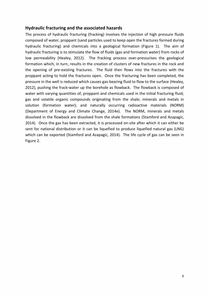
The process of hydraulic fracturing (fracking) involves the injection of high pressure fluids
composed of water, proppant (sand particles used to keep open the fractures formed during
hydraulic fracturing) and chemicals into a geological formation (Figure 1). The aim of
hydraulic fracturing is to stimulate the flow of fluids (gas and formation water) from rocks of
low permeability (Healey, 2012). The fracking process over-pressurises the geological
formation which, in turn, results in the creation of clusters of new fractures in the rock and
the opening of pre-existing fractures. The fluid then flows into the fractures with the
proppant acting to hold the fractures open. Once the fracturing has been completed, the
pressure in the well is reduced which causes gas-bearing fluid to flow to the surface (Healey,
2012), pushing the frack-water up the borehole as flowback. The flowback is composed of
water with varying quantities of; proppant and chemicals used in the initial fracturing fluid;
gas and volatile organic compounds originating from the shale; minerals and metals in
solution (formation water); and naturally occurring radioactive materials (NORM)
(Department of Energy and Climate Change, 2014e). The NORM, minerals and metals
dissolved in the flowback are dissolved from the shale formations (Stamford and Azapagic,
2014). Once the gas has been extracted, it is processed on-site after which it can either be
sent for national distribution or it can be liquefied to produce liquefied natural gas (LNG)
which can be exported (Stamford and Azapagic, 2014). The life cycle of gas can be seen in
Figure 2.
7
Figure 1. Schematic diagram of the hydraulic fracturing process as carried out in the US. Not to scale. (From ProPublica, Granberg, 2015).

8
Figure 2. Simplified flow chart of the lifecycle of gas. The black boxes represent the stages that are unique to shale gas and the grey boxes represent stages unique to liquefied natural gas. (From Stamford and Azapagic, 2014).
The overall hydraulic fracturing operation, which includes the process of hydraulic fracturing
and associated industrial processes (e.g., water transport, well installation), pose potential
hazards to the environment. In geological terms, there is a likelihood of seismic activity as
large amounts of fluid are being injected into the Earth, thus modifying the in-situ stress
conditions resulting in the potential re-activation of faults (Healey, 2012). There is also
concern about the potential for the fracturing process to cause groundwater contamination
if the fractures intersect with permeable pathways (e.g., mineral veins or pre-existing fracture
networks) potentially allowing upwards migration of fluids (gas and possibly liquids) into less
deeply buried geological formation that might contain groundwater (Myers, 2012). Industrial
processes that can potentially impact upon the environment include the quantity and
composition of the fluids used during drilling and fracturing. Waste products (fluids, fugitive
emissions and drilling waste) also pose an environmental hazard if not properly treated and
disposed of. In addition, the integrity of the well is also a key concern as a loss of well integrity
can potentially lead to groundwater contamination (Jackson, 2014) and fugitive gas
emissions. Over the long term (years) the process of well abandonment becomes significant
because, even after it has been abandoned, the well can still pose a risk to the environment
through corrosion of any remaining casing or degradation of the cement, leading to well
integrity being compromised (Vengosh et al., 2014). There is the potential for groundwater
contamination and fugitive gas emission if well abandonment is not completed properly
(Osborn et al., 2011). The risk of adverse health effects associated with emissions, waste
products and groundwater contamination is also, sometimes, held to be of concern (Shonkoff
et al., 2014; Werner et al., 2015).
9
Earthquakes
Seismic activity can either be natural, i.e., movement of faults as a response to natural
changes in the in-situ stress state or of the mechanical properties of rocks in the Earth’s crust,
or can be induced, i.e., by human activities such as mining or fluid injection (Styles and Baptie,
2012).
Seismic activity in the UK
Seismic activity within the UK is relatively low when compared to other countries (The Royal
Society and the Royal Academy of Engineering, 2012). Earthquakes of magnitude ML4.0 (ML
means local magnitude) on the Richter Scale take place once approximately every 3-4 years
and events of magnitude 5.0 take place once every 20 years (The Royal Society and the Royal
Academy of Engineering, 2012). According to the British Geological Survey (BGS), who
operate and maintain a network of approximately 100 seismic monitoring stations (National
Earthquake Monitoring System) throughout the UK, the majority of the seismic activity is
around magnitude 1.5, which is at the detection limit of the BGS’ national monitoring system.
Hundreds of these earthquakes take place in the UK every year; however, on account of the
depth at which the earthquake takes place, very few are actually felt by the general
population. In essence, because of geometrical spreading (inverse-square law), the greater
the depth at which the earthquake takes place, the less chance there is of the effects being
felt at the ground surface, especially for small events.
Seismic activity caused by industrial activities
Davies et al. (2013) carried out an extensive review of seismic events induced by industrial
activities, these are summarised in Table 1 and Figure 3. The authors compiled evidence
dating from 1933 to the date of publication. They found 198 possible examples of induced
seismicity. However, they point out that, because they restricted their search to published
examples, their database cannot be considered comprehensive. They also do not account for
every seismic event in an earthquake swarm; they only report the largest magnitude event
during the swarm.

10
Table 1. Table displaying the types of industrial activities associated with earthquakes. The range of magnitudes associated with each activity is also shown. (From Davies et al., 2013).
Industrial activity Earthquake magnitude range
Mining 1.6-5.6
Oil and gas extraction 1.0-7.3
Water injection into oil wells 1.9-5.1
Waste disposal 2.5-5.3
Reservoir impoundment 2.0-7.9
Boreholes drilled by academic institutes 2.8-3.1
Solution mining 1.5-5.2
Geothermal operations 1.0-4.6
Hydraulic fracturing 1.0-3.8
Figure 3. Graph displaying the magnitude vs. frequency of felt seismic events induced by industrial activities. Note that the maximum magnitude of events associated with hydraulic fracturing is 4. (From Davies et al., 2013).
From examination of Table 1 and Figure 3, it is clear that the maximum magnitude of seismic
events associated with hydraulic fracturing are lower than those associated with the majority

11
of other industrial drilling / mining activities. It should be noted that there is no documented
evidence of seismic events originating from hydraulic fracturing being large enough to cause
structural damage or of inducing subsidence (Green et al., 2012). Of more significance is the
larger maximum seismic magnitude of events associated with waste fluid disposal into deep
geological formations. The Department of Energy and Climate Change’s (DECC) document on
water management during shale gas operations (Department of Energy and Climate Change,
2014e) presently makes no mention of whether this type of waste water disposal is permitted
in the UK.
The BGS has identified a multitude of instances of seismic activity being caused by other
industrial activities. Some of the best-documented examples are those associated with coal
mining in Nottinghamshire. Between mid-December 2013 and April 2014, 93 earthquakes of
maximum magnitude of 1.8 ML were detected around the New Ollerton area of
Nottinghamshire (Figure 4) (British Geological Survey, 2014). The area has a history of seismic
activity associated with local coal mining operations and the recent seismic events are also
considered to be related to this (British Geological Survey, 2014).
Figure 4. Map of the New Ollerton earthquake activity dating from 2000. (From British Geological Survey, 2014).

12
Historically, seismicity associated with abandoned coal mines in the UK has not exceeded a
magnitude of 3.0 ML (British Geological Survey, 2014). The maximum magnitude of seismic
events associated with shale gas activities are considered to be similar to that of coal mining
(Figure 3). However, the hypocentres (depths of origin) of coal mine related seismicity will
likely be shallower than shale gas related events. Therefore, a coal mining related event of
the same magnitude as a shale gas related event is more likely to be felt because even deep
coal mines only extend to half the depth that hydraulic fracturing of shale will extend.
Therefore, the same event will feel less strong from the greater depth on account of
geometric spreading. There are also no reports of mining related seismic activity resulting in
structural damage but there is evidence of superficial damage, e.g., cracks in plaster,
occurring as a result of mining-induced seismic activity (British Geological Survey, 2014).
Evidence from the US also indicates that seismic activity associated with coal mining is of a
magnitude similar to that of the maximum magnitude associated with shale gas operations.
For instance, Emery County, Utah, US, has a well-documented history of coal mining related
seismic activity (e.g., Arabasz et al., 2005; Fletcher and McGarr, 2005; McGarr and Fletcher,
2005). The maximum magnitude of such events is considered to be 3.9 ML (Arabasz et al.,
2005). This is comparable to the maximum magnitude of events associated with hydraulic
fracturing (3.8 ML) (Davies et al., 2013).
Seismicity is known to be induced by industrial activities other than coal mining. For instance,
the process of extracting geothermal energy has been documented as a cause for earthquakes
that are, potentially, larger than those caused by coal mining if the process takes place in
crystalline rock (igneous and metamorphic) as opposed to sedimentary rock (Evans et al.,
2012). One type of geothermal energy extraction, hot-dry-rock (HDR), involves the drilling of
two deep wells into hot regions of the Earth’s crust. The wells are then fractured and cold
water is pumped down through one of the wells. The water migrates through the fractures
connecting the two wells, during which time it takes heat from the fracture walls, and returns
to the surface at the other well. The process of fracturing and fluid migration can result in
seismic activity.
HDR geothermal energy exploration in the UK has been carried out at Rosemanowes Quarry,
near Penryn, Cornwall. The site, which was in operation between 1978 and 1991, originally
consisted of two wells drilled into granite to a depth of approximately 2 km and separated by
0.17 km, an additional well was drilled in 1985 (Evans et al., 2012). Local natural seismicity is
low, but there has been seismic activity associated with operation of the site. The largest
tremor was a 3.5 ML event which took place in 1981. This event was part of a cluster of
earthquakes that occurred 6 km south of the site, near the town of Constantine (Evans et al.,
2012). Initial fracturing using gel and water injection methods resulted in thousands of small
tremors of <0.16 ML, none of which were felt by the local population or site workers (Evans
et al., 2012).

13
In terms of the rest of Europe, the maximum recorded magnitude of earthquakes associated
with geothermal energy exploration and extraction from crystalline rocks is 3.5 ML (Evans et
al., 2012). This occurred at the Monte Amiata geothermal area of Italy where wells are drilled
to 3 km depth into metamorphic rocks (Evans et al., 2012). In Europe there has been some
effort to stimulate geothermal production from sedimentary rocks, however, very little in the
way of induced seismic activity has been documented. Of the activity that has been
documented, the largest recorded magnitudes have been 3.0 ML which occurred at
Larderello-Travale and Torre Alfina, both in Italy. The wells in each of these locations were
drilled to a depth of 2 km into carbonate rocks (Evans et al., 2012).
Seismic activity and hydraulic fracturing
Induced seismicity is generally accepted to occur when seven predefined criteria, as defined
by Davis and Frohlich (1993), are satisfied. These seven criteria are (Davies et al., 2013):
1. The seismic events are the first to be recorded in the area.
2. There is a time correlation between injection of fluid into the rock and the seismic
activity.
3. The epicentres are within 5km of the operation site.
4. The earthquakes occur at / around the depth of injection.
5. If tremors do not occur around the depth of injection, are there any geological
structures that may allow flow of fluid to the event hypocentre?
6. Are the changes in fluid pressure at the base of the well sufficient to permit
earthquakes?
In order for an earthquake to be induced due to hydraulic fracturing, a fault must be present
that satisfies three key factors: a) it must be already critically stressed; b) it must be able to
accommodate a large amount of the fracturing fluid (i.e. it must be sufficiently hydraulically
conductive for fluid injection into the fault to occur) and; c) it must be composed of rock
strong and brittle enough to allow seismic failure (Green et al., 2012).
Two types of seismic events are known to be associated with the process of hydraulic
fracturing (The Royal Society and the Royal Academy of Engineering, 2012). Smaller,
microseismic events are associated with the formation of new fractures, while movement
along pre-existing, pre-stressed faults can result in larger seismic events. In terms of scale,
microseismic events are faint events that cannot be felt on the Earth’s surface. The maximum
magnitude of the microseismic tremors is 0 on the moment magnitude scale; for comparison,
a felt earthquake has a moment magnitude on the order of 3 (Halliburton, 2011). These larger
earthquakes occur when the fracturing fluid migrates through the rock and along a pre-
14
existing fault and decreases the pressure holding the fault together, this allows the fault to
move, resulting in an earthquake. The magnitude (energy release) of the event is dependent
upon the size of the fault, the elastic stiffness of the rock and the amount by which the fault
slips. In the case of hydraulic fracturing, the stimulation is the volume of fluid that flows
through the fault.
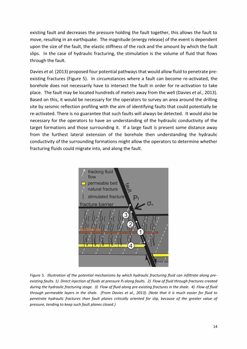
Davies et al. (2013) proposed four potential pathways that would allow fluid to penetrate pre-
existing fractures (Figure 5). In circumstances where a fault can become re-activated, the
borehole does not necessarily have to intersect the fault in order for re-activation to take
place. The fault may be located hundreds of meters away from the well (Davies et al., 2013).
Based on this, it would be necessary for the operators to survey an area around the drilling
site by seismic reflection profiling with the aim of identifying faults that could potentially be
re-activated. There is no guarantee that such faults will always be detected. It would also be
necessary for the operators to have an understanding of the hydraulic conductivity of the
target formations and those surrounding it. If a large fault is present some distance away
from the furthest lateral extension of the borehole then understanding the hydraulic
conductivity of the surrounding formations might allow the operators to determine whether
fracturing fluids could migrate into, and along the fault.
Figure 5. Illustration of the potential mechanisms by which hydraulic fracturing fluid can infiltrate along pre-
existing faults. 1) Direct injection of fluids at pressure Pf along faults. 2) Flow of fluid through fractures created
during the hydraulic fracturing stage. 3) Flow of fluid along pre-existing fractures in the shale. 4) Flow of fluid
through permeable layers in the shale. (From Davies et al., 2013). (Note that it is much easier for fluid to
penetrate hydraulic fractures than fault planes critically oriented for slip, because of the greater value of
pressure, tending to keep such fault planes closed.)

15
In order to understand fully and evaluate the risk of earthquakes, the in-situ rock stresses and
the fracture network within the fracturing area must be established (Healey, 2012). The
operator is obliged by law to conduct a geophysical survey of a site for evidence of any large
faults (i.e., those that are visible on a seismic reflection profile) that, if stimulated, could
trigger an earthquake. With the resulting data, the operator can then take reasonable steps
to avoid any interaction with the fault throughout both the drilling and fracturing stages
(Department of Energy and Climate Change, 2014d).
Once drilling has been completed, the operator is prohibited from carrying out exploratory
fracturing until a series of small test hydraulic fractures are carried out. If these are successful,
and there is no evidence of enhanced seismic activity, the operator can begin the main
exploratory hydraulic fracturing stage (Department of Energy and Climate Change, 2014d).
DECC requires the installation of real-time seismic monitoring systems on-site (Department
of Energy and Climate Change, 2014b). DECC states that any seismic activity that occurs
during the operation of the well must be reported. The operator is responsible for this as well
as the mitigation and monitoring of any activity (Department of Energy and Climate Change,
2014b).
At the Preese Hall site (Cheshire, UK. Operated by Cuadrilla Ltd.) two small earthquakes took
place in April of 2011 (for more information, see the Preese Hall section of this report) the
causes of which were the subject of a number of investigations (de Pater and Baisch, 2011;
Green et al., 2012; Styles and Baptie, 2012). The investigations recommended the
introduction of a traffic light system to monitor and mitigate any potential risks posed by
earthquakes caused by hydraulic fracturing. This traffic light system has been adopted by
DECC (Table 2) with the limit for acceptable induced seismic activity being set at magnitude
0.5. This threshold equates to the normal background seismic activity caused by the passing
of trucks, trains or farming vehicles. It is above the magnitude frequently associated with
hydraulic fracturing and as such might act as a precursor to larger events (Department of
Energy and Climate Change, 2014d). Due to the lack of shale gas operations that have taken
place, there is no information regarding the practical implementation of this system, and it
likely that setting the limit for cessation of operations at ML = 0.5 is very conservative and may
be unfeasibly low. However, DECC have stated that they will keep up to date with new
research on the levels of seismic activity associated with hydraulic fracturing and adjust the
magnitude thresholds accordingly (Department of Energy and Climate Change, 2014d).
Table 2. Table displaying the traffic light system in place for shale gas exploration in the UK. (Adapted from Department of Energy and Climate Change, 2014d).
Traffic light colour
Magnitude
Action taken
Green <0.0 Regular operation of well.

16
Amber 0.0-0.5 Injection proceeds with caution. Potentially reduce injection
volume. Increase intensity of monitoring.
Red >0.5 Immediately stop injection and fracturing, bleed off the well
and continue monitoring.
The Preese Hall reports also suggested two mitigation methods that might be applied if
induced seismicity is detected. The first method is to limit the amount of fluid that enters the
shale and the injection rate after the fracturing has taken place. This involves an immediate
reduction of well pressure upon completion of the fracturing operation, thus allowing as
much fluid as possible to flow back to the surface. The second involves reducing the volume
of fluid used during the fracturing process (Green et al., 2012).
Seismic activity monitoring techniques
Detection of the number, and magnitude, of earthquakes depends on two main factors: the
proximity of the monitoring station to the epicentre of the seismic event and; the quality of
the monitoring equipment (Davies et al., 2013). Both factors will determine the number of
events and the lowest magnitude limit that can be detected (Davies et al., 2013). The closer
the monitoring station is to the epicentre, and the higher the quality of the detection
equipment, the larger will be the number of smaller tremors that can be detected. Increasing
the number and sensitivity of monitoring stations in close proximity to the source of the
events will increase the detection resolution. In the case of shale gas operations, this will
involve installing monitoring stations around the areas where hydraulic fracturing takes place.
In order to establish background levels of seismic activity around the operation site,
monitoring systems should be installed prior to any drilling taking place. It should be noted
that in order to constrain the location of an event, the same event must be detected by at
least three monitoring stations or preferably more detection at only one or two stations will
not be sufficient.
A significant point made by Davies et al. (2013) is that, due to the fact that the detection of
earthquakes is so dependent upon the placement and quality of the seismic monitoring
stations, comparisons of detected earthquakes between sites is very limited unless
monitoring systems and their placement are identical.
There are many methods of monitoring seismic activity. These include:
Tiltmeters – These are highly sensitive instruments that measure tilt (or rotation) of
the Earth’s surface near faults (United States Geological Survey, 2014). Electronic
tiltmeters are similar to a spirit level; they contain a compartment filled with
conductive fluid and a bubble (United States Geological Survey, 2009). Rotation of the
Earth’s surface causes the bubble to move, which provides a measure of the degree
of tilt (United States Geological Survey, 2009)
17
Microseismic – This technique involves the measurement of small-scale earthquakes
(events of <0.0 ML) that are of too low a magnitude to be felt at the surface (EGS
Solutions, 2015). This is also a passive technique; this means that it requires no seismic
vibration trucks or explosives that are commonly used in active seismic exploration
(Microseismic, 2014). The detectors (geophones or accelerometers) are arranged in
arrays across the area of interest. They can be installed on the surface, at shallow
burial depths or down monitoring wells (Microseismic, 2014). The installations can
either be permanent or temporary depending upon the needs of the operator. During
the hydraulic fracturing period, the technique allows the operators to map, both
horizontally and vertically, where the fractures are occurring underground. Any
seismic events that take place during the remainder of the operation can be detected
in the same way.
As with most issues relating to shale gas operations, the risks associated with induced
seismicity will vary from site to site. As a result, the type and density (number) of monitoring
stations will be varied from site to site depending on factors such as the level of background
seismicity. Despite the lack of shale gas exploration activity in the UK, some seismic
monitoring of sites has taken place (see the Preese Hall Case Study section) one example of
which is the monitoring carried out at the drilling site at Balcombe, West Sussex, operated by
Cuadrilla Resources Ltd. This monitoring was carried out by members of the University of
Bristol (Horleston et al., 2013). Four broadband seismometers were installed 1 month before
drilling took place (Figure 6). Monitoring was carried out prior to, and during, the drilling
operation. The objective of the monitoring was to establish background levels of seismic
activity and noise in addition to examining the detectability thresholds of the equipment.

18
Figure 6. Map displaying the location of the four monitoring stations (yellow pins, BA01-BA04) in relation to the Balcombe drilling site (red pin). Note that the fourth monitoring station (BA04) was located in close proximity to the approximately NW-SE trending train line. Image is about 1.5 km across. (From Horleston et al., 2013. Reproduced in accordance with Google fair use policy).
Data was continuously collected at all four stations from 1st of July through to 25th of
September 2013. This covered the period one month prior to drilling (in order to establish
the seismic background) and the full duration of the operation. The data was first examined
for seismic event triggers using a computer algorithm. A total of 134 were detected, however,
manual re-examination revealed that none could be classified as seismic events and that all
could be attributed to increased background noise (Horleston et al., 2013).
Results show that the largest and most significant source of seismic noise was that of train
movements originating from the London to Brighton rail line which was located 150m from
the fourth monitoring station (BA-04) (Figure 6) (Horleston et al., 2013). The level of
perceived vibration intensity produced by such train movements equates to the intensity of
a magnitude 1.5 earthquake originating at 3 km depth over a more prolonged period (note:
intensity describes how a tremor is perceived people and objects at the Earth’s surface,

19
whereas magnitude measures energy released at the source). The remaining sources of
seismic noise were other surface factors including cars, people, animal movements and
weather. However, these produce different frequencies and signal shapes that allow them
to be differentiated from earthquakes (Horleston et al., 2013).
When drilling began, the general level of background noise increased. As would be expected,
the monitoring station nearest to the drill site displayed the largest increase in background
(Horleston et al., 2013). In terms of detection limits, Horleston et al. (2013) estimate that the
minimum magnitude that could automatically be detected by the array and computer
algorithm was -0.2. The authors note that this is slightly lower than the limit of what is
required for implementation of the traffic light monitoring scheme.
The report highlights the importance of appropriate monitoring site selection. Sites need to
be located at an appropriate range of distances from the drilling site whilst at the same time
avoiding pre-existing noise. For example, the similarity between felt intensities at the surface
arising from a 0.5 ML earthquake occurring at depth and train movements on the surface
could result in the masking of a seismic event if it were to take place as a train was passing
(Horleston et al., 2013). Although this is unlikely, it is still a point worth making as a tremor
of this magnitude would cause the halting of any operation under the current traffic light
monitoring system. Horleston et al. (2013) also recommend that a real-time monitoring
system be installed at each site. Because of the need for rapid analysis of seismic data and
the need to differentiate between background noise and seismic events, the authors raise the
point that, based on their lower detection limit being near to that required under the
proposed traffic light system, the UK may not currently be in a position accurately to predict
seismic events rapidly enough to allow hydrofracturing to be halted before more events take
place. The fact that the felt intensity arising from train movements, albeit detected at a
monitoring station near to a train track, can be larger than that required to halt fracturing
demonstrates this point.
According to the authors, the UK’s recording of seismic events by the BGS is only complete to
a minimum magnitude of 2.0 ML, or possibly 1.5. Using the Gutenberg-Richter relationship
for the UK, the authors estimate that there is the potential for 5,000 natural earthquakes per
year in the UK that would trigger an amber warning and 2,000 that would trigger a red
warning. This highlights the need for thorough baseline monitoring prior to any fracturing
taking place, the difficulty of recognising induced seismicity at this level relative to
background and the potential need for revision of the limits set in the traffic light system as
experience is acquired.
The potential for subsidence due to shale gas extraction
DECC (Department of Energy and Climate Change, 2014d) consider that there is minimal risk
of subsidence resulting from the natural gas extraction process. Even after the drilling of

20
hundreds of thousands of wells in the US, there is currently no documented evidence of
subsidence resulting from shale gas extraction (Department of Energy and Climate Change,
2014d). On the other hand, subsidence has been associated with coal mining activities due
to the fact that large amounts of material are removed from the subsurface (Singh and Yadav,
1995). Shale gas operations will remove an extremely small volume of material from the
subsurface, therefore the risk of subsidence can be considered negligible. Subsidence can
also happen when sufficiently porous rock is compressed at high enough pressures to begin
to collapse the porosity, but shale is a low-porosity rock that is not easily compressed and will
therefore be unable to collapse and cause subsidence.
21
Contamination
Water
A concern amongst the general public is the perceived potential for water contamination to
occur as a result of hydraulic fracturing. Ground and surface water contamination is
intimately linked with other aspects, including preparation of the site, i.e., the drilling phase,
well integrity problems, well abandonment and management of waste residues and the risk
they pose for water contamination.
Before proceeding with the discussion of water contamination and shale gas operations, it is
worth considering exactly what an aquifer is. An aquifer is simply a permeable water-bearing
rock formation, regardless of whether or not it is exploited for potable water. Most UK
aquifers are not exploited but potable water is drawn from rivers and surface reservoirs
instead. Two thirds of the UK domestic water supply is drawn from surface water sources.
It should also be noted that drilling through aquifers is not an uncommon occurrence in the
UK, as shown in Figure 7 (Davies et al., 2014). Between 1902 and 2013, 2152 hydrocarbon
wells have been drilled in the UK. 428 (20%) have been drilled through highly productive
aquifers and 535 (25%) were drilled through moderately productive aquifers (Davies et al.,
2014).

22
Figure 7. Map of the UK showing the location of intergranular flow and fracture flow aquifers together with a) the location of onshore exploration wells, and b) potential shale gas and oil-bearing formations. (From Davies et al., 2014).
Potential contaminants in water
A variety of chemicals are used in the hydraulic fracturing fluid. The most common additives
are shown in Table 3. The amounts and types of chemicals added to the fluid varies from site
to site. However, in all cases, the aim is to optimise the hydraulic fracturing process and
maximise gas recovery. In the US, the main additives are friction reducers (polyacrylamide)
designed to allow the fracturing fluid to be pumped into the well at an increased rate; this is
known as “slickwater” fracturing.

23
Table 3. Table displaying the chemicals generally used in the hydraulic fracturing fluids together with their purpose and downhole results. (From Frac Focus, 2015b).
The chemicals in the fluid are subject to assessment by the appropriate environmental
agency. The details of the chemicals, together with the reason for their use and associated
hazards, must be fully disclosed. This is subject to the protection of intellectual property of
the operators (Department of Energy and Climate Change, 2014e). However, it is in the
interests of the operators to publically disclose all chemicals as it helps gain public trust and
aids transparency. In the US, a chemical disclosure registry (www.fracfocus.org) has been set
up. Members of the public can look up any registered well and find the composition of the
fluid used during the fracturing process together with information on well depth and water
volume used. A similar, centralised, platform has been put in place in Europe by the
International Association of Oil and Gas Producers (http://www.ngsfacts.org/findawell/). The
website lists the shale gas wells that have been fractured since 2011 by operators that
participate in the Natural Gas from Shale Facts website (http://www.ngsfacts.org/), a website
providing factual information on hydraulic fracturing). The website provides the location,
permitting information and the substances used in the fracturing process. However,
disclosure of information about wells is voluntary.
There is some debate around the composition of the hydraulic fracturing fluids, mostly
concerning the chemical additives. For instance, a report by the Tyndall Centre for Climate
Change put the typical chemical content of the fluid at 2 vol%; this translates to 180-580 m3
24
of chemicals per well mixed into the fracturing fluid (Wood et al., 2011). This concentration
is higher than the estimates suggested in the Royal Society report (0.17 vol%) (Stamford and
Azapagic, 2014). The amount of chemicals introduced into the well, based on this estimate,
is 4.5-14.5 m3. It should be noted that current drilling in the UK is still at the exploratory stage
and the composition of the fluid may change if the operators move into the production stage
(Stamford and Azapagic, 2014). It should also be noted that the composition of the hydraulic
fracturing fluid will vary from site to site on account of factors such as variations in local
geology, well depth and well length.
Water usage during shale gas operations
The process of drilling and hydraulic fracturing consumes large amounts of clean water which
must be sourced by the operator either from a local utilities company or from local
ground / surface water sources. Before utility companies provide water to the drilling site,
they must be satisfied that supplying the requested amount of water will not put domestic
water (and other customers’) supplies at risk (Department of Energy and Climate Change,
2014e). Nonetheless, it should be noted that this is no different to other industries which
require water. The permission to extract water from nearby surface water or groundwater
sources is dependent upon the operator obtaining a permit to do so from the appropriate
environmental agency. The main criteria that must be met in order for a licence to be granted
is that the water supply in the area must be sustainable (Department of Energy and Climate
Change, 2014e), it must also not impact adversely on other users and the environment. A
further factor that needs to be considered is the exact time when the water will be needed
on-site. The operation will not require a constant supply of water, but rather will require
larger amounts of water at particular times, i.e., during drilling and at the start of the hydraulic
fracturing stage (The Royal Society and the Royal Academy of Engineering, 2012).
The amount of water required to conduct hydraulic fracturing is considerable, although it is
not as water intensive as some other industries, e.g., beverage and food production, and
paper production (Department of Energy and Climate Change, 2014e). It is estimated that
each well will require between 10,000 and 30,000 m3 (10,000 to 30,000 tonnes or 2 to 6
million gallons) of water over the course of the operation (Logan et al., 2012). Most of this
water will be required in the drilling and hydraulic fracturing stages, i.e., 1-2 months. UK
operator, Cuadrilla, estimates that 12,000 m3 of water will be required over the life span of a
well (House of Commons Energy and Climate Change Committee, 2011). This equates to the
same amount of water required to run a coal-fired power station for 12 hours, or to water a
golf course for one month (The Royal Society and the Royal Academy of Engineering, 2012),
or the amount lost each hour by United Utilities from leakages.
Vengosh et al. (2014) pointed out that a potential way to reduce the impact on the domestic
water supply would be to use alternative water sources as a base for the drilling mud and
hydraulic fracturing fluid. The authors suggested that low quality water, such as brackish

25
water or water from acid mine drainage, could be used. However it is uncertain whether such
water would be available in the quantities needed for hydraulic fracturing. There is evidence
that when acid mine drainage waters are mixed with Marcellus Shale flowback, various
dissolved salts are formed that can act to capture contaminants within both fluids (Kondash
et al., 2014). However, the effect that these already contaminated waters might have on the
physical properties of the fracturing fluid is unknown. Perhaps an unreasonable amount of
chemicals may need to be added to the fluid in order for it to have the same properties as
fracturing fluid prepared with uncontaminated water as the base. This could offset the
environmental benefits of reducing the stress on the domestic water supply.
During the drilling stage a fluid known as “drilling mud” is permanently circulated through the
borehole. The fluid is pumped down the drill string and exits the drill bit, at high pressure,
through nozzles. It then travels back to the surface around the gap between the drill string
and the wall rock, known as the annulus. This process acts to lubricate and cool the drill bit
whilst loosening and collecting fragments of rock resulting from the drilling, known as
“cuttings” (Williamson, 2013). The drilling mud transports the cuttings to the surface, thus
allowing the drill bit to function properly and not become clogged up. In addition, a powdered
mineral, barium sulphate (barite), is added to the drilling mud to increase the density of the
fluid so that the hydrostatic pressure created by the mud column is greater than the reservoir
pressure. This prevents hydrocarbons from the reservoir from flowing into the borehole
(Williamson, 2013). The hydrostatic pressure also helps to stabilise the borehole, by
counteracting the forces due to depth of burial that make the borehole want to close up.
Once returned to the surface, the fluid passes through a shaker that separates the larger
cuttings from the drilling mud. The mud then passes through a series of tanks that remove
the smaller cuttings through hydrocylones or centrifuges and apply chemical treatment to
maintain the desired specifications, thus allowing the fluid to be recycled (Williamson, 2013).
The most commonly used fracturing fluid consists of a water base (approximately 90 to 93%)
together with sand proppant (approximately 5 to 8% by volume) and chemicals (1-2%). The
base can also be foam, oil or acid. Which of these is chosen depends upon the depth to the
formation of interest. For instance, shallow, low-pressure reservoirs can be fractured with
foams created using N2 or CO2 while acids are used in reservoirs mainly consisting of
carbonate rocks (Holditch, 2006). Oil-based fluids are used when fracturing takes place in
close proximity to formations that are sensitive to water damage (Montgomery, 2013).
However, depending on the oil used, there is the potential for the flowback to be more highly
contaminated and hence require more treatment before being disposed of. However, it is
unlikely that an oil-based fracturing fluid would be permitted in the UK.
Vidic et al. (2013) highlighted concerns around the fate of hydraulic fracturing fluid. Two
major questions they raised based on their literature review were; 1) what happens to the
water that does not return to the surface as flowback or production water, and 2) could the
non-recovered water eventually contaminate aquifers (Davies, 2011; DiGiulio et al., 2011;
26
Boyer et al., 2012; Myers, 2012; Warner et al., 2012). One potential fate of the fracturing
fluid is that it is absorbed into the shale. A previous study of Marcellus Shale well logs has
shown that the rock contains little free water (Engelder, 2012), therefore there is the
potential for the fluid to enter the rock. There is also potential for fluid to migrate upwards
along gaps between the casing and cement or along fractures in the rock formations, although
this requires a suitable pressure gradient.
Current US National Energy Technology Laboratory research
The US Department of Energy (DOE) and the US National Energy Technology Laboratory
(NETL) are currently funding three projects examining alternative, non-water-based
stimulation techniques. The projects are as follows (National Energy Technology Laboratory,
2015e);
Development and field testing of novel natural gas surface process equipment for
replacement of water as primary hydraulic fracturing fluid. This project involves the
use of wellhead (produced) natural gas that has been liquefied and compressed, as
the primary constituent of hydraulic fracturing fluid. If successful, this may prove to
be a more cost-efficient non-water / CO2 based stimulation technology that can be
used instead of, or in parallel with, traditional water-based methods. The benefits of
such fracturing fluids include less waste production, reduced need for water transport
and better production through reduced clay swelling and blockages in the producing
formation. The project is due to finish in October 2017 (National Energy Technology
Laboratory, 2015a).
Development of nanoparticle-stabilized foams to improve performance of water-less
hydraulic fracturing. This project aims to develop surface-treated nanoparticles
capable of stabilizing foam fracturing fluids, the main constituents of which are
commonly used in fracturing fluids (CO2, N2, water and liquefied petroleum gas).
Nanoparticles treated with surface coatings could provide long term stability for
foamed fracturing fluids. This, in turn, can reduce water usage. In addition, their small
size means that they can stabilize foams with much smaller bubble sizes, and hence
permit an increase in the viscosity of the foam. This has the added benefit of allowing
proppant to be carried in the foam. Another benefit of using nanoparticles is that the
type of treatment and concentration of the particles themselves can be tuned to a
particular system. For example, the particles can be tuned to allow the proppant to
be carried into the fractures at which point the foam structure will break, this
facilitates flowback without re-foaming of the fluid. The project is due to finish in
October 2016 (National Energy Technology Laboratory, 2014).
Development of non-contaminating cryogenic fracturing technology for shale and
tight gas reservoirs. The project aims to study, test and develop cryogenic fracturing
technology using CO2 or liquid nitrogen. If successful, this research will increase the
27
permeability of, and therefore recovery from, shale gas reservoirs. In addition to
increasing production, this technique can reduce, or even eliminate, water usage,
whilst also reducing damage to the target formation and reducing any potential for
groundwater contamination by eliminating the need for additives in the fracturing
fluid. The project is due to end in July 2016 (Research Partnership to Secure Energy
for America, 2013).
Ways that water contamination can take place
The Groundwater Foundation, a US-based group, cite a number of potential mechanisms of
groundwater contamination. These include leaks from storage tanks, septic systems, landfills,
chemicals and road salts (The Groundwater Foundation, 2015). When considering the
potential for water contamination from shale gas activities, the contamination risk from these
other sources must be considered in order to provide a perspective on the severity of any
hazard posed and the associated risks to humans and animals.
In the shale gas industry, storage tanks are used on-site to store water and waste fluids.
Outside of the shale gas industry, storage tanks can be located both above and below ground
and can contain a variety of fluids, including other hydrocarbons. Over time, and without
proper inspection and repair, these can leak and potentially result in contamination of surface
and / or groundwater (The Groundwater Foundation, 2015). The Groundwater Foundation
say that there are as many as 10 million storage tanks in the US, these are likely to be for both
commercial (e.g., fuel storage at petrol stations and chemical storage at factories) and private
use (e.g., on farms). One would presume that those at commercial sites would be subject to
regular checks to ensure that no cracks are appearing, however, this may not be the case for
storage tanks in private use. This could potentially increase the risk of leaks, and hence of
water contamination. In terms of shale gas operations, on-site storage tanks will fall under
the first category and should be periodically inspected. This should reduce the hazard to
acceptable levels. To mitigate this hazard further, drilling and fracking sites are routinely
covered with geotextile membranes designed to contain any spills or leakages. This was
observed to be the case at the US sites visited by the Task Force in March of 2015. Bunds and
additional ground membrane protection can be used in areas of chemical storage to mitigate
further against spills.
Septic tanks, particularly those on private properties not connected to the main sewage
system, can also present a significant risk to surface and groundwater if not properly
designed, constructed, located or maintained (The Groundwater Foundation, 2015). A leak
from one of these tanks could result in the discharge of human waste, and the chemicals used
to treat it, into the local groundwater system.
Landfill sites have previously been shown to have the potential to cause groundwater
contamination through migration of leachates (meteoric fluid (i.e. rainwater) that percolates

28
through waste and leaches contaminants) (e.g., Barker et al., 1988; Monteiro Santos et al.,
2006; Mor et al., 2006). Modern landfills are sealed against leaks by first laying down a layer
of low permeability clay. A synthetic membrane layer is then placed over the top of the clay.
This is an impermeable layer that prevents any leachates migrating into the surrounding rock
and causing contamination. These linings can, with time, degrade and crack, thus allowing
leachates to move into the surrounding clay and increasing the risk of contamination.
Chemicals, such as fertilisers and pesticides used on farmland, and road salts also have the
potential to contaminate surface water and groundwater (e.g., Levallois et al., 1998; Babiker
et al., 2004). The process of eutrophication occurs when excessive quantities of chemical
fertilizers are used on crops. These fertilizers can enter surface waters via runoff or can
percolate through the soils and can enter into shallow aquifers. Once in surface waters, the
chemicals encourage the growth of algae on the water’s surface. This results in the oxygen
content of the water decreasing and the hazard to aquatic species increasing. Salts used to
de-ice roads during cold periods can migrate into the groundwater system, resulting in
elevated chloride levels (e.g., Williams et al., 2000; Godwin et al., 2003). This is a particular
problem in areas that require regular de-icing during cold periods, i.e., urban areas and
motorways (The Groundwater Foundation, 2015).
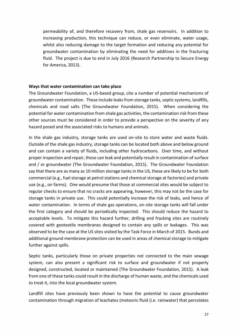
Well integrity Wells consist of a number of barriers, i.e., casing, cement, valves and seals, which prevent the
unplanned escape of fluid from the well (Davies et al., 2014). In the UK, DECC state that a
well must have at least three layers of casing; an outer conductor or surface casing, an
intermediate casing that extends down below the aquifer and an inner production casing
which runs into the geological formation of interest (Figure 8) (Department of Energy and
Climate Change, 2014c). It is this latter section in which the hydraulic fracturing takes place.
For information on the drilling and fracturing process at Preese Hall, see the Case Study
section. The operator can add further layers of casing to improve the well stability and further
reduce risks of well leakage.
Well integrity refers to the isolation of gas originating from the target formation and the
formations through which the well passes (Jackson, 2014). A failure in well integrity involves
the failure of one or more barriers that leads to the formation of a pathway that allows
leakage of liquids and / or gases from the well into the surrounding environment (King and
King, 2013) or along the outer wall of the well casing. It is worth noting that a barrier failure
will not necessarily lead to a failure in well integrity as a complete pathway may not be
formed. Only failure of all barriers will result in a leak path forming. A barrier failure is one
that does not lead to complete loss of integrity. For instance, a single layer of casing can fail
but none of the fluid within the well may leak out into the surrounding rocks, therefore,
overall well integrity is maintained.
29
Figure 8. Schematic diagram of the design of a shale gas well. Not to scale. (From Stamford and Azapagic, 2014).
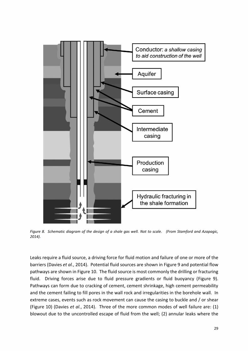
Leaks require a fluid source, a driving force for fluid motion and failure of one or more of the
barriers (Davies et al., 2014). Potential fluid sources are shown in Figure 9 and potential flow
pathways are shown in Figure 10. The fluid source is most commonly the drilling or fracturing
fluid. Driving forces arise due to fluid pressure gradients or fluid buoyancy (Figure 9).
Pathways can form due to cracking of cement, cement shrinkage, high cement permeability
and the cement failing to fill pores in the wall rock and irregularities in the borehole wall. In
extreme cases, events such as rock movement can cause the casing to buckle and / or shear
(Figure 10) (Davies et al., 2014). Three of the more common modes of well failure are: (1)
blowout due to the uncontrolled escape of fluid from the well; (2) annular leaks where the

30
fluids can move upwards along the outside of the outer well casing or gaps within the layers
of the well casing and radial leaks; and (3) where the well casing fails and the fluid leaks into
the surrounding rocks (Figure 9) (The Royal Society and the Royal Academy of Engineering,
2012).
Figure 9. Schematic diagram of the potential sources of fluid that can enter the well casing if a failure of well integrity takes place. 1) Gas-rich coal formations. 2) Non-producing permeable gas reservoir. 3) Biogenic or thermogenic gas in a shallow aquifer. 4) Gas from the target reservoir. (From Davies et al., 2014).
31
Figure 10. Schematic diagram displaying the potential pathways along which fluid can exit the well, resulting in leaks. 1) Through the annulus between cement and wall rock. 2) Between layers of casing and cement. 3) Between the cement plug and casing. 4) Through the cement plug. 5) Through the cement. 6) Through the cement then along the boundary between the cement and the casing. 7) Along the plane of weakness caused by shearing of the wellbore. (From Davies et al., 2014).
Well installation methods
The following section outlines the steps taken by operators during installation to ensure that
well integrity is established and maintained.
Casing centralisation
Effective centralisation of the casing is critical to achieving good cementation. The correct
installation of both allows the casing to be properly supported; prevents fluids from leaking
to the surface; and allows production zones and water bearing zones to be properly isolated
(PetroWiki, 2014a). There are two common methods of centralising casing during the
installation process; the use of (a) bow-spring and (b) rigid type centralisers (Figure 11). The
former method is the most popular and can be used when the borehole is enlarged. On the
other hand, if the borehole is only slightly larger in diameter than the casing, rigid centralizers

32
are used. Rigid centralizers are also frequently used when installing the casing in the
horizontal sections of wells (PetroWiki, 2014c).
Figure 11. Schematic diagrams (not to scale) of the two main centraliser types used in the oil and gas industry. Left: Rigid centralizer. Right: Bow-spring centralizers. Note that the dimensions of the centralizers will vary depending on which casing layer is being installed. (From Halliburton, 2006a, b).
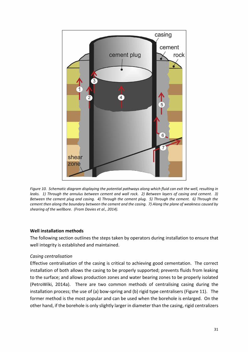
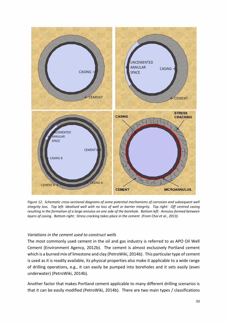
Effective casing centralisation is also crucial for ensuring well integrity as the
non-centralisation of casing within the borehole can leave an area of un-cemented casing if
mud is not properly displaced during the cementing process (Figure 12 top right). This sort of
gap should be routinely detected by the operators (see Well Integrity Testing section below)
and remedial action should take place. If, however, the re-cementing is not carried out
properly, fluid can be trapped in the annulus and interact directly with the casing. This will
likely result in severe corrosion and an increase in the risk of well failure (Choi et al., 2013).
33
Figure 12. Schematic cross-sectional diagrams of some potential mechanisms of corrosion and subsequent well integrity loss. Top left: Idealised well with no loss of well or barrier integrity. Top right: Off centred casing resulting in the formation of a large annulus on one side of the borehole. Bottom left: Annulus formed between layers of casing. Bottom right: Stress cracking takes place in the cement (From Choi et al., 2013).
Variations in the cement used to construct wells
The most commonly used cement in the oil and gas industry is referred to as APO Oil Well
Cement (Environment Agency, 2012b). The cement is almost exclusively Portland cement
which is a burned mix of limestone and clay (PetroWiki, 2014b). This particular type of cement
is used as it is readily available, its physical properties also make it applicable to a wide range
of drilling operations, e.g., it can easily be pumped into boreholes and it sets easily (even
underwater) (PetroWiki, 2014b).
Another factor that makes Portland cement applicable to many different drilling scenarios is
that it can be easily modified (PetroWiki, 2014b). There are two main types / classifications

34
of Portland cement that are produced; these are the American Society for Testing Materials
(ATSM) and American Petroleum Institute (API) (PetroWiki, 2014b). The ATSM cement
classification is mainly used in the construction industry, and therefore will not be considered
further. The API classification, on the other hand, applies only to cement used in the
construction of oil and gas wells. The API cement classification has a number of sub-classes
dependent upon the chemical composition of the slurry. API cement can be Class A through
to J (excluding I) with classes G and H being the most commonly used (Table 4) (Crook, 2006;
PetroWiki, 2014b). The composition of typical Class G and H Portland cements can be seen in
Table 4, a comparison between carbon compounds in different cement classes and the effect
that varying the amount of specific compounds makes, is shown in Table 5. More detailed
information about the chemical composition and material properties of the cements can be
found in Appendix 1. Based on the information presented in the below tables, it is clear that
the optimum cement will vary from site to site.
Table 4. Table displaying the depth and special conditions that dictate which API Class of cement can be used in a given well. (From King, 1996).
API Class
Depth to base of well (m) Special conditions for use
A 1830 None
B 1830 Sulphate resistance required
C 1830 Finer grind giving high early strength
D 1830-3050 High pressure and temperature conditions
E 3050-4270 High pressure and temperature conditions
F 3050-4880 Extremely high temperatures
G 2440 Can be mixed with additives and used over a range of temperatures and depths
H 2440 Can be mixed with additives and used over a range of temperatures and depths
J 3600-4880 High pressure and temperature conditions and can be mixed with additives
Table 5. Table displaying the carbon compound content of the various API Classes of cement. The effect of varying the carbon compound content is also shown. Note that under the phase composition section, C is an

35
abbreviation of CaO; S is and abbreviation of SiO2; A is an abbreviation of Al2O3; and F is an abbreviation of Fe2O2. (From Crook, 2006).
For the cement to be pumped to the base of the well, i.e., >3 km distance, additives are
introduced into the slurry in order to control the density which, in turn, controls the rock
formation pressure during setting, setting time, flow properties, and when set, the strength
(Environment Agency, 2012b). This also represents one of the reasons why Class G and H
cements are the most popular in the oil and gas industry as their physical properties can be
easily modified through the introduction of such additives (Crook, 2006).
Accelerators, e.g., CaCl2, NaCl, KCl and Na2SiO3 are one type of additive. These act to alter the
time required for the cement to harden and set. These are particularly useful in areas of low
temperature country rock where adding an accelerator will result in a more efficient drilling
and cementing phase (Crook, 2006).
Retarders are most commonly used in the Class A, C, G and H cements. These serve the
purpose of extending the thickening time of the cement. Note that the thickening time is the
time required to mix and pump the cement slurry. Examples of retarders include
36
lignosulfonates, cellulose derivates, hydroxycarboxylic acids, organophosphates and
inorganic compounds (e.g., borax (Na2B4O7∙102) and ZnO) (Crook, 2006).
Lightweight additives, also known as extenders, can be added to API Class A, C, G and H
cements. When the cement slurries are mixed to these API Classes, the resulting slurry can
be too dense (i.e., >15 lbm/gal (pound mass per US gallon)) to allow efficient circulation
(Crook, 2006). The addition of extenders solves this problem by reducing the density of the
cement (Crook, 2006).
There are three common types of extenders; physical, pozzolanic and chemical (Crook, 2006).
One common physical extender is bentonite gel. Bentonite is a colloidal clay (i.e. the mineral
group including montmorillonite [NaAl2(AlSi3O10)∙2OH]). Attapulgite
[Mg,Al)2(OH/Si4O10)∙12H2O], a salt gel, is also used in slurries with high salt content.
Attapulgite is a mineral with a fibrous crystal habit (shape) not dissimilar to asbestos. Because
of this, its use has been banned in some countries but not in the UK. Perlite (silica rich volcanic
glass), crushed coal and ground rubber are also used (Crook, 2006). One or more of these
extenders may be added to any one slurry.
Pozzolanic extenders have a lower specific gravity than the standard API Class slurries;
therefore, by adding them to the mix, the density of the slurry is reduced whilst the
consistency of the slurry remains approximately unaltered (Crook, 2006). Four main types of
pozzolanic extenders are used; fly ash (a mix of SiO2+Al2O3+Fe2O3), microspheres (hollow, gas
filled silica rich aluminosilicate glass spheres), microsilica (high surface-area vitreous silica and
SiO2 mix) and diatomaceous earth (diatom skeletons) (Crook, 2006).
Gypsum (hydrated calcium sulphate) and sodium silicate are the two most commonly used
chemical extenders. The latter is much more effective at lowering the slurry density than
other extenders, particularly bentonite, therefore less needs to be used (Crook, 2006).
Weighting agents do the opposite of extenders, i.e., increasing the density of the slurry
(Crook, 2006). This is required in situations where wells are highly pressurised and require a
slurry of higher density. Haematite (Fe2O3), ilmenite (FeOTiO2), hausmannite (Mn3O4) and
barite (BaSO4) are the main weighting agents used, with haematite being the most common
(Crook, 2006).
Dispersants, or friction reducers, are used to control the flow properties of the slurry and
reduce frictional pressure during pumping. The two main dispersants are polyunsulfonated
naphthalene and hydroxycarboxylic acids (i.e., citric acid) (Crook, 2006).
Fluid-loss-control additives (FLAs) are used to maintain the fluid volume of the slurry (Crook,
2006). This is significant as many of the other physical properties of the slurry depend upon
the water content. Using FLAs ensures that the water content, and hence physical properties,
remain consistent. The materials used as FLAs can be broadly categorised as either water-
soluble or water-insoluble. Water-insoluble FLAs are either bentonite or polymer resins while

37
water-soluble FLAs can be natural polymers, cellulosics or vinylinic-based polymers (Crook,
2006).
Also of note is the fact that cement slurries can be “foamed” through the introduction of a
foaming agent, foam stabilizers and a gas, usually nitrogen, into the slurry. This creates a low
density slurry that, when properly mixed, forms a very stable and lightweight cement
containing discrete air bubbles that do not coalesce (Crook, 2006).
Corrosion of casing and degradation of cement
Depleted oil and gas wells are favourable sites for CO2 capture and storage (CCS). This process
involves the injection of large amounts of the carbon dioxide, produced from the burning of
fossil fuels, into the Earth. The other common method of CCS is to inject the CO2 into deep
saline aquifers (Carbon Capture & Storage Association, 2015). Over longer timescales (i.e.,
years), a concern the companies responsible for carrying out carbon storage have is the
potential for loss of barrier and well integrity. If a loss of boundary cement integrity occurs
and CO2 is allowed to come into contact with the casing, corrosion can take place (Choi et al.,
2013). If sufficient interaction takes place, complete well integrity failure can occur, resulting
in CO2 leaking into the surrounding rock formations (Choi et al., 2013). It should be kept in
mind that the information presented in the remainder of this section has been obtained from
academic publications related to CCS and not shale gas extraction. Therefore, caution must
be used when applying the results to shale gas operations. However, these studies are useful
in giving an indication of the potential risks.
Carey et al. (2010) carried out an experimental study on corrosion along the interface
between steel well casing and cement in a synthetic system with a fluid composed of 50:50
CO2 and NaCl-rich brine. They found that both the cement and casing were affected and that
the fluid had penetrated as far as 250 µm into the cement. The casing showed clear signs of
corrosion that penetrated 25-30 µm into the steel. Precipitates of both calcium and iron were
found on the casing surface, these were considered to represent the products of corrosion.
The rate of corrosion front propagation was calculated to be between 0.4-1.0 mm/yr.
Talabani et al. (2000) discussed the four main types of casing corrosion that can take place in
wells. The first was erosion corrosion which most commonly occurs during, or shortly after,
drilling has taken place and the casing has been inserted in to the borehole. Wear and
abrasion of the casing occurs when salts and oxides are formed or deposited on the surface
of the casing. The risk of casing corrosion taking place can be minimised by carrying out
cementing as soon as possible after the casing has been introduced into the borehole. The
second way corrosion can take place is through evolved hydrogen diffusion into the casing
resulting in embrittlement, and subsequent failure. The third mechanism of corrosion is
through localised growth of bacteria colonies on the casing as these can alter the chemistry
of the casing surface. For example, some bacteria are able to reduce sulphate, producing H2S
38
which can accelerate the rate at which steel corrosion takes place (Sherar et al., 2011). In the
upper areas of the well where multiple layers of casing are present, galvanic corrosion can
take place if the annulus is not properly cemented and a gap forms between two layers of
casing (Figure 12, bottom left). If this annular gap contains an electrolyte (e.g., Na+, Ca2+,
Mg2+) then the casings will effectively connect electrically with one of the casings acting as an
anode (Choi et al., 2013). The overall result is enhanced corrosion. Choi et al. (2013) noted
that if this type of corrosion does take place, it cannot easily be repaired.
Choi et al. (2013) also described ways in which cement can effectively repair itself over time.
For instance, stress cracks in the cement create pathways for fluids to interact with casing
(Figure 12, bottom right). Upon injection of CO2 into the well, reactions can take place with
the cement to form CaCO3 which can fill the cracks. However, this appears to be exclusive to
CCS and the more complex nature of the fluids used during hydraulic fracturing mean that
this type of self-healing is highly unlikely to take place.
Well integrity testing
Detection of barrier or well integrity failure can be carried out by testing for pressure
retention within the casing, known as “sustained casing pressure” at the ground surface
(Davies et al., 2014). This involves increasing the internal pressure of the well to the
operational pressure and observing for any loss of pressure (The Royal Society and the Royal
Academy of Engineering, 2012). A drop in pressure indicates that well integrity has been
compromised. However, this method does not indicate whether complete well failure has
taken place or at what depth failure has taken place. Failure of the cement, leading to the
formation of channels, can be detected through a number of tests. Any fluids that leak from
the well and migrate up through the annulus between the cement and wall rock can be
detected by inserting probes into the soil directly adjacent to the well. Sampling nearby
groundwater can also reveal any leaks (Davies et al., 2014).
Formation Integrity Tests (FIT) can also give an indication of well integrity. This test was
undertaken at the Preese Hall site. It is carried out after the casing has been cemented in
place but before the next section is fully drilled. The operator drills down through the cement
plug at the base of the previous section, drilling continues into the underlying formation but
only for a few tens of meters and the drill is withdrawn. Similarly to the sustained casing
pressure test, FIT involves closing the blowout protector and pumping drilling fluid down the
wellbore at progressively higher pressures, up to the maximum pressure used during drilling.
This, in turn, applies hydraulic pressure to the newly drilled rock and the cement at the
bottom of the previous hole section (Cuadrilla Resources Ltd, 2012). FIT tests give an
indication of any leaks, and hence any problems with the cement or casing installation, while
also providing evidence as to whether the next formation will allow fluids to flow into it. The
FIT is an industry standard test that allows the determination of what is known as the
“equivalent mud weight” (i.e., the optimal average mud weight (in pounds per gallon (ppg) to
39
be used in the drilling fluid) required during the next drilling stage to prevent the collapse of
the borehole due to the pressure of the surrounding rock and to control the reservoir pressure
and prevent in influx of hydrocarbons (Cuadrilla Resources Ltd, 2012).
A cement bond log (CBL) is the main way of testing the quality of the cement job in the
production section and allows identification of any areas that require remedial cementing.
This test was carried out at Preese Hall. As long as properly carried out, CBL tests can give
highly reliable estimates of well integrity and zonal isolation (PetroWiki, 2014a). The tests
work on the principle that acoustic wave amplitude is rapidly attenuated in good cement, but
not attenuated when the cement is poor, i.e., partially bonded (PetroWiki, 2014a). The
quality of a cement job can be divided into one of four scenarios (PetroWiki, 2014a);
1. Free pipe - No cement between casing and cement.
2. Good bond - Cement is properly bonded to the casing and rock formation.
3. Bond to casing only - Cement is bonded to the casing but not the formation.
4. Partial bond. - Space exists within an otherwise well-bonded casing
The CBL test involves lowering a piece of equipment, consisting of sonic transmitters and
receivers, down the wellbore and measuring how well the cement has bonded to the casing
and the wall rock. This is done by transmitting sonic waves through the cement and casing of
the well. Any gaps in the cement will be detected and appear on the resulting log. Cuadrilla
point out that the equipment is highly sensitive and can detect gaps as little as 0.05 mm wide
that are too thin to transmit fluid. They say that even if the cement mix is perfect and
complete filling of the annulus takes place (as shown by cement returning to the surface) the
CBL will still pick up these anomalies (Cuadrilla Resources Ltd, 2012).
There is a number of limitations with conventional CBL techniques. These are outlined in
Table 6. A more modern technique that has been developed is that of radial-cement
evaluation which was developed in order to overcome some of the limitations of conventional
CBL techniques (PetroWiki, 2014a). These devices use at least one azimuthally sensitive
transducer to evaluate the quality of a cement job around the circumference of the casing.
The devices can also use ultrasonic tools to evaluate the cement job by determining the
acoustic impedance of the material outside the casing; if the cement job is good and the
cement is well bonded to the casing, the impedance is high; if the job is poor and there is poor
bonding, the impedance is low (PetroWiki, 2014a). Utilising this ultrasonic technique avoids
the problem of surface roughness and residual cement on the interior of the casing. A major
advantage of this technique is that azimuth “maps” of the cement quality around the
circumference of a well can be generated (PetroWiki, 2014a). Despite these advantages,
radial-cement evaluation is still sensitive to gas that may be trapped in any microannuluses
that form between the cement and casing (PetroWiki, 2014a). This is a problem that is also
faced by conventional CBL techniques.

40
Table 6. Table outlining the limitations of conventional CBL techniques. (PetroWiki, 2014a).
A number of additional tests are carried out to ensure that the well is functioning correctly
(e.g., a blowout preventer test) and that it can withstand the maximum differential pressure
experienced by the well (positive and negative pressure tests). The 2012 UK Oil and Gas
(UKOG) (Oil and Gas UK, 2012) well integrity guidelines say that the testing procedure should
include the success / failure criteria and the reaction to trends, e.g., an increase in annular
pressure.
Pressure testing should be carried out with liquid where possible. Preferably, this should be
water as the use of drilling mud or other fluids containing solids can hide the presence of
small leaks.
The blowout preventer test (also known as a seal assembly test) is carried out to test the
integrity of the interface between the casing and the wellhead (National Commission on the
BP Deepwater Horizon Oil Spill and Offshore Drilling, 2011). To carry out the test, a packer is
installed below the seal assembly which isolates the area around the top of the well and the
seal assembly. The blowout preventer is sealed and the pressure within the well is raised.
The well passes the blowout preventer test if the pressure within the isolated part of the well
remains approximately constant (National Commission on the BP Deepwater Horizon Oil Spill
and Offshore Drilling, 2011). A drop in pressure indicates that there is a leak, and therefore
that the well fails the test.
A positive pressure test involves sealing off the production casing by closing valves in the
blowout preventer. This is designed to test the well’s ability to hold pressure. The pressure
is initially raised to between 200-300 psi within the production casing at which point the
pumps are stopped and the pressure held constant (National Commission on the BP
Deepwater Horizon Oil Spill and Offshore Drilling, 2011). This is known as a low pressure test.
These are important because low pressures are usually a more severe test for equipment
designed to operate at high pressures; failure at low pressures should not pose a safety
hazard; and the barrier has to seal at low pressures (Oil and Gas UK, 2012). If the pressure
remains constant, the well is considered to have passed the low pressure test. The pumps
are then restarted and the pressure increased to the full test pressure and held for a second

41
time (Oil and Gas UK, 2012). As with the low pressure test, if the pressure holds, the well
passes the positive pressure test.
Negative pressure tests (also known as inflow or drawdown tests) are essentially the inverse
of a positive pressure test (National Commission on the BP Deepwater Horizon Oil Spill and
Offshore Drilling, 2011). During the test, the pressure within the well is reduced to a level
below that of the surrounding rock formation (National Commission on the BP Deepwater
Horizon Oil Spill and Offshore Drilling, 2011). This is intended to test whether hydrocarbons
from the target rock formation will flow into the well. The test is failed if the pressure within
the well increases when the well is sealed, or if flow from the well takes place when the well
is open (National Commission on the BP Deepwater Horizon Oil Spill and Offshore Drilling,
2011). In a successful negative pressure test, there should be no pressure increase and no
flow from the well, i.e., the pressure remains approximately constant within the well
(National Commission on the BP Deepwater Horizon Oil Spill and Offshore Drilling, 2011). This
test determines the quality of the wellhead assembly, casing, mechanical seals and cement
seals; it is the only pressure test that evaluates the integrity of the primary cement seals
(National Commission on the BP Deepwater Horizon Oil Spill and Offshore Drilling, 2011).
Geochemistry can also be used to monitor well integrity. As demonstrated previously, a
potential mechanism for monitoring the integrity of hydraulic fracturing wells is through the
use of isotopic measurements of radioactive tracers in flowback fluid and groundwater.
Warner et al. (2014) hypothesised that injection of hydraulic fracturing fluid into shale results
in specific radioactive isotopes entering the fluid. If well integrity is compromised and a leak
occurs, the concentration of these isotopes in ground water should increase.
To investigate this, the authors aimed to establish the chemical and isotopic composition of
both the flowback fluid and the groundwater. By doing this, one can establish whether
flowback fluids have a unique geochemical fingerprint. This, in turn, allows leaks in the well
casing to be identified. Warner et al. (2014) examined water samples from shale gas wells
drilled in the Marcellus Shale and from the surrounding Appalachian basin water supply. They
found that, although the geochemical signature of the flowback fluid is similar to that of the
water produced from other oil and gas wells, the flowback had distinct lithium (δ7Li) and
boron (δ11B) geochemical signatures compared to the ratios (Li/Cl and B/Cl). The ratios were
found to be consistent across the Marcellus Shale. The reason for these two elements in
particular being of higher concentration is thought to be due to either the interaction of
fracturing fluid with clays in the shale, brine trapped within the shale and boron associated
with organic matter. The flowback fluid was characterised by higher B/Cl and Li/Cl ratios
together with lower δ7Li and δ11B values. The current literature search has not revealed any
evidence of this specific technique being applied elsewhere. A problem with this technique
is that it relies on the analysis of groundwater to determine whether a leak has taken place.
Thus, once a leak has been detected, contamination would have already taken place.
42
Evidence of well integrity failure in the UK
There is no evidence of well integrity failure associated with onshore shale gas wells in the
UK, perhaps due to the limited amount of drilling that has taken place. As a result, evidence
of onshore well integrity comes from conventional hydrocarbon wells. Between 2000 and
2013, the EA recorded nine onshore incidents of pollution associated with the release of crude
oil within 1 mile of the well in question (Davies et al., 2014). Of these nine incidents, two
were associated with well integrity problems, both of which took place at the Singleton Oil
Field in 1993. The current operator by IGas but the field was under different ownership when
the incidents occurred. The failure was detected via groundwater monitoring. A failure
adequately to cement the conductor and intermediate casings (Figure 8) led to a leak, the
magnitude of which was not stated. In terms of environmental impact, no air or land
contamination occurred and minor water contamination was found (Davies et al., 2014). An
investigation, overseen by the Environment Agency (EA), began in 1997 and the source of the
leak was identified. Remedial action was taken and d monitoring has been continued at the
site. Currently, levels of contamination are within the acceptable range set by the EA (Davies
et al., 2014). The other leaks were caused by problems with the pipeline linked to the well.
No leaks were reported from abandoned sites. However, a caveat to this is that abandoned
wells in the UK are currently not monitored and pollutants that are less obviously visible, for
instance colourless and odourless methane, are less likely to be reported (Davies et al., 2014).
It is evident that this lack of monitoring will have to change if shale gas exploration goes ahead
in the UK.
Evidence of well integrity failure in the US
Estimates from the Marcellus shale in Pennsylvania suggests that barrier integrity failure took
place in 3.4% of wells (219 of 6466) drilled between 2008 and 2013 (Vidic et al., 2013). Of the
4602 wells drilled between 2010 and 2012, 7% (320) displayed a loss of integrity (Ingraffea,
2012). However, the latter author gave no indication of how many of these wells that
experienced barrier integrity failure required remedial action or constituted contamination
incidents. This was consistently higher than the failure rate of conventional wells drilled
during the same time period. The cause of failure was deemed to be a combination of poorly
installed, insufficient and defective cement and / or casing. Ingraffea (2012) highlighted the
fact that well integrity was not improving with time, suggesting that the US operators were
not adhering to best operating practices or regulations were not being successfully enforced.
Ingraffea et al. (2014) conducted an in-depth review of 75,505 compliance reports for 41,381
conventional and unconventional oil and gas wells drilled in Pennsylvania, USA, between
January 2000 and January 2013 with the aim of investigating failures in well integrity through
casing and cement problems. Wells associated with shale gas exploration and extraction

43
exhibited a six fold increase in the incidence of cement and / or casing problems when
compared to problems associated with conventional wells.
Wells drilled between 2000 and 2012 associated with both conventional and unconventional
oil and gas wells displayed a rate of cement and / or casing failure of 1.9% across the entirety
of Pennsylvania. Conventional wells displayed a 1.0% failure rate while 6.2% of
unconventional wells lost integrity over the same timeframe. However, upon closer
examination, it is apparent that there are clear geographical differences in the failure rates.
For instance, the majority of unconventional wells are located in the north-eastern area of
the state. Wells located here had a much higher failure rate; 5.21% of conventional wells
drilled between 2000 and 2009 failed, while after 2009, 2.27% of wells lost integrity compared
to 0.73% and 2.08% of wells drilled in the remainder of the state over the same timeframes.
The same was also the case for unconventional wells. Wells drilled prior to 2009 in north-
eastern counties exhibited a failure rate of 9.84% which dropped to 9.14% for wells drilled
after 2009. This is a substantial increase over the rest of the state where failure rates of 1.49%
and 1.88% are observed for unconventional wells drilled pre-2009 and post-2009 respectively
(Ingraffea et al., 2014). The authors suggest that the high occurrence of well failures in
unconventional wells in the northeast of the state between 2000 and 2009 may be attributed
to the fact that the industry was inexperienced in drilling the Marcellus Shale. In addition,
only 61 unconventional gas wells were drilled during this period. Therefore, the failure rates
may be unreliable on account of the small sample size. However, the small reduction in failure
rates in the 2,714 unconventional wells drilled since 2009 suggest that this is not the case
(Ingraffea et al., 2014).
The authors attributed the increased failure rate in post-2009 unconventional wells to
increased pressure on the operator to start production as soon as possible, resulting in the
installation process, and consequently well integrity, being compromised. However, the
authors point out that the increased failure rate could also be due to human factors such as
increased awareness of the issue of well integrity leading to well inspectors carrying out a
more thorough job (Figure 13) (Ingraffea et al., 2014). Indeed, in the US, the percentage of
wells that are inspected within the first year of operation increased from 76% prior to 2009
to 88.7% after 2009 (Ingraffea et al., 2014). It also has to be considered that if a well is found
to have a leak; future inspections may be more thorough, resulting in an increased chance to
find leaks, particularly smaller ones that may have been missed by less thorough inspections.
With this in mind, the authors warn against direct comparison between failure rates between
old and new wells without these factors being considered.
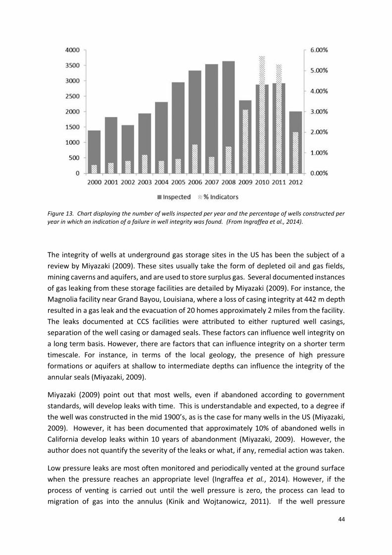
44
Figure 13. Chart displaying the number of wells inspected per year and the percentage of wells constructed per year in which an indication of a failure in well integrity was found. (From Ingraffea et al., 2014).
The integrity of wells at underground gas storage sites in the US has been the subject of a
review by Miyazaki (2009). These sites usually take the form of depleted oil and gas fields,
mining caverns and aquifers, and are used to store surplus gas. Several documented instances
of gas leaking from these storage facilities are detailed by Miyazaki (2009). For instance, the
Magnolia facility near Grand Bayou, Louisiana, where a loss of casing integrity at 442 m depth
resulted in a gas leak and the evacuation of 20 homes approximately 2 miles from the facility.
The leaks documented at CCS facilities were attributed to either ruptured well casings,
separation of the well casing or damaged seals. These factors can influence well integrity on
a long term basis. However, there are factors that can influence integrity on a shorter term
timescale. For instance, in terms of the local geology, the presence of high pressure
formations or aquifers at shallow to intermediate depths can influence the integrity of the
annular seals (Miyazaki, 2009).
Miyazaki (2009) point out that most wells, even if abandoned according to government
standards, will develop leaks with time. This is understandable and expected, to a degree if
the well was constructed in the mid 1900’s, as is the case for many wells in the US (Miyazaki,
2009). However, it has been documented that approximately 10% of abandoned wells in
California develop leaks within 10 years of abandonment (Miyazaki, 2009). However, the
author does not quantify the severity of the leaks or what, if any, remedial action was taken.
Low pressure leaks are most often monitored and periodically vented at the ground surface
when the pressure reaches an appropriate level (Ingraffea et al., 2014). However, if the
process of venting is carried out until the well pressure is zero, the process can lead to
migration of gas into the annulus (Kinik and Wojtanowicz, 2011). If the well pressure
45
increases directly after the well has been vented, the leak is considered to be high pressure
and remedial action should be taken. This can involve re-cementing the problem area (known
as cement squeeze), pumping polymer gels into the problem areas (gel squeeze), sealing the
leak using packers or topping off the cement (Ingraffea et al., 2014).
Current US National Energy Technology Laboratory research
The US Department of Energy (DOE) and National Energy Technology Laboratory (NETL) are
currently funding four projects related to well integrity and zonal isolation, all of which are
due to end between December 2015 and October 2017. The projects are as follows (National
Energy Technology Laboratory, 2015e);
“Nanite” for better well-bore integrity and zonal isolation. Nanite is a cementitious
material containing a functionalised nanomaterial additive that, when mixed into the
cement slurry, can transform cement into a smart material capable of sensing and
responding to stress, pressure and temperature changes in addition to any change in
cement composition. Changes can be detected through electrical, acoustic and
electromagnetic measurements (National Energy Technology Laboratory, 2015c).
Development of nanite will allow information regarding cement barrier integrity,
direct measurements of casing stress, cement shrinkage and well conditions
throughout the life-cycle of the well and identify any infiltration of gas / fluid / wall
rock into the cement.
nXis well integrity inspection in unconventional gas wells. This project involves the
development of a combined X-ray / neutron backscatter imaging device capable of
providing information about well and barrier integrity that is of higher accuracy than
the currently available techniques (National Energy Technology Laboratory, 2015d).
MCIP - this project is focused on improving the current methods of remediating
leaking wells through the use of microbially-induced calcite precipitation (MICP).
MICP has been shown previously to be capable of sealing a downhole fracture in
sandstone. However, it has yet to be seen whether this can be applied to poorly
cemented wells (National Energy Technology Laboratory, 2015b).
Annular isolation in shale gas wells: prevention and remediation of sustained casing
pressure and other isolation breaches. This project aims to develop techniques to
improve groundwater contamination mitigation, to improve failed well seal
remediation, to improve annular isolation during well construction and to develop
techniques to avoid annular seal failure (Research Partnership to Secure Energy for
America, 2014).

46
Evidence of water contamination
The issue of groundwater contamination has proved to be a contentious one in the US. For
instance, there have been studies carried out in the areas overlying the Marcellus Shale,
Appalachian Basin, Pennsylvania that examined the potential for contamination of
groundwater by methane (Osborn et al., 2011; Jackson et al., 2013; Molofsky et al., 2013;
Darrah et al., 2014). This contamination has been proposed to be directly linked to shale gas
drilling and hydraulic fracturing (Osborn et al., 2011). However, there are other studies that
have disputed the claims made in these investigations (e.g., Molofsky et al., 2013).
In an extensive review of the published information on the hazards and risks posed to water
resources by shale gas exploration and extraction carried out by Vengosh et al. (2014), four
main areas of hazard were cited;
1. Contamination of shallow aquifers by fugitive methane and saline deep formation
waters which can result in groundwater becoming salinated.
2. Spills or leaks of inadequately treated flowback and wastewater on the surface
and / or leaks from joints in pipes and from storage tanks, this can result in
contamination of shallow groundwater and surface water.
3. Accumulation of either radioactive elements or toxins in sediments and soils near
disposal, leak or spill sites resulting in contamination.
4. Over-extension of the water supply due to the high demand for water during the
hydraulic fracturing stage that can lead to water shortages and conflicts with other
water uses.
A significant challenge with regard to determining the risk of groundwater contamination
taking place involves the issue of groundwater flow rate. Shale gas drilling in the US has only
accelerated dramatically since the early 2000’s, but the rate of groundwater flow is too slow
for any large scale contamination to have yet become apparent (Vengosh et al., 2014).
However, there is evidence of groundwater contamination from conventional oil and gas
extraction that dates back much further, thus providing a potential indication of how
contamination could take place or develop in future (Vengosh et al., 2014).
Water contamination associated with industrial activity
There is evidence for groundwater contamination taking place in other industrial settings
directly linked to energy production. For instance, the process of harnessing geothermal
energy has been shown to result in groundwater contamination in Turkey (e.g., 2000; Dogdu
and Bayari, 2005; Aksoy et al., 2009). Aksoy et al. (2009) attributed the contamination to four
mechanisms;
47
(a) natural upwards movement of geothermal (hot) fluids along faults, driven by
expansion during cooling,
(b) accelerated upwards migration of fluids due to poorly constructed boreholes,
(c) faulty reinjection applications and
(d) uncontrolled discharge of waste products into the local drainage network.
They also cited contamination by heavy metals (e.g., arsenic, antimony and boron) as the
most significant potential contaminant associated with geothermal energy.
Coal mines have also been demonstrated as being a source for groundwater contamination
through acid mine drainage (e.g., Johnson and Hallberg, 2005; Akcil and Koldas, 2006; Bhuiyan
et al., 2010). Acid mine drainage refers to the process of water flowing through active or
abandoned mines and, in the process, leaching both heavy metals from the surrounding rock
formations and acidic slats that have built up in the wall rock (Johnson and Hallberg, 2005).
Waste produced from mining operations can also be a source for acidic, heavy metal enriched
fluids if inappropriately stored or disposed of, i.e., left open to the atmosphere at the Earth’s
surface.
Water contamination associated with shale gas operations
There exists the remote possibility that fractures created during the hydraulic fracturing
process can penetrate into shallow groundwater. The fractures can act as conduits for
fracturing fluids, gas and other contaminants to enter the aquifer. The risk of this taking place
is minimal enough to be considered acceptable as hydraulic fracturing usually takes place
kilometres below the aquifer and the fractures typically extend, mainly laterally, to a few
hundred meters (Davies et al., 2012; Department of Energy and Climate Change, 2014c). In
addition, a pressure gradient is established around the rock formation when hydraulic
fracturing takes place, this means that flow into the well will preferentially take place, not
flow away from the well.
The largest vertical hydrofracture propagation reported from US hydraulic fracturing
operations is 588m (Davies et al., 2012) (see Text Box 1 for a discussion of what controls the
vertical extent of fractures). By analysing data from five US shale formations, the authors
determined that the probability of a fracture propagating vertically more than 350m is
approximately 1%. The data was obtained from previous microseismicity studies. However,
the authors did not have access to the primary data set. This introduces uncertainties in the
presented results. Firstly, measurements of the vertical extent of the fractures were made
directly from the published graphs. This decreases the likelihood of the resolution of the
smaller fractures. Further, the resolution of fractures smaller than 100m is limited owing to
the technical limit on maximum fracture resolution attainable by the microseismic analysis.
The impact of these uncertainties is that there is considerable error in the recognition and
measurements of fractures smaller than 100m. It is likely that the number of smaller fractures
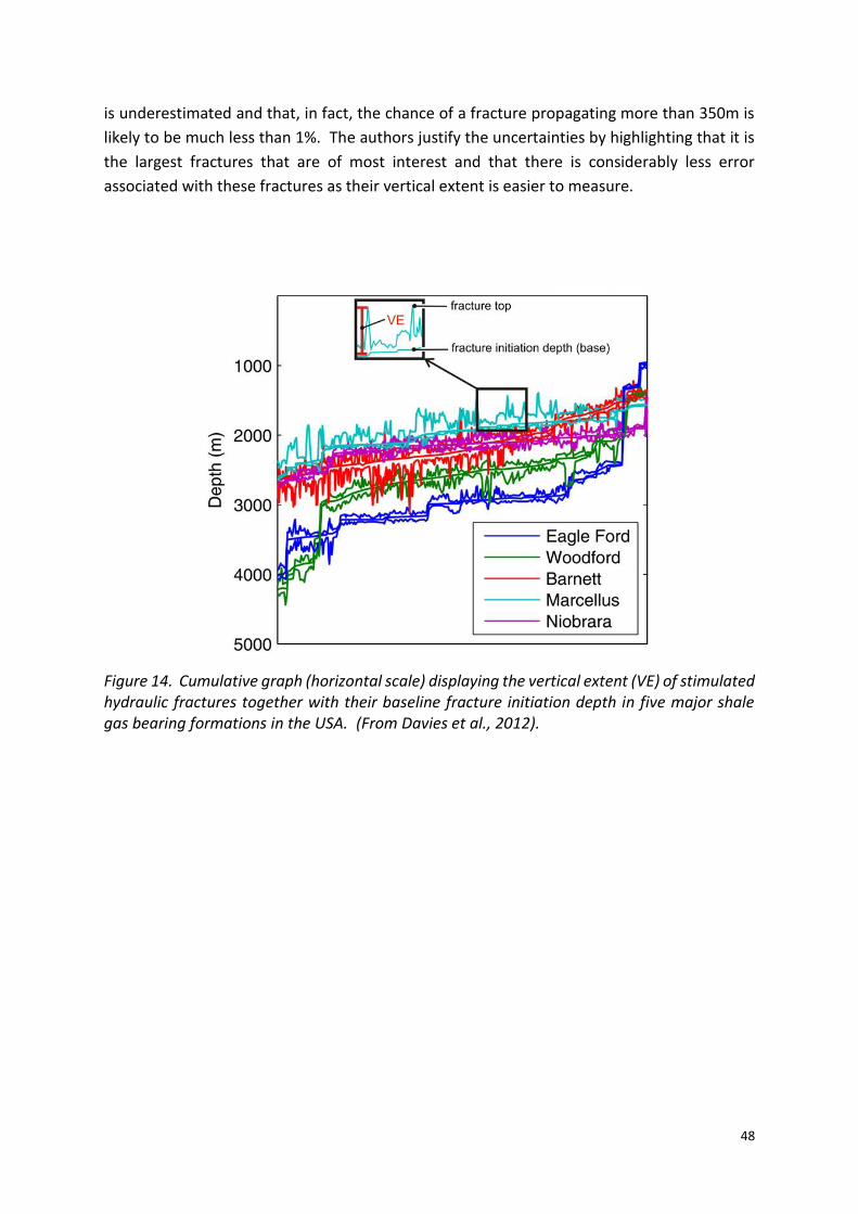
48
is underestimated and that, in fact, the chance of a fracture propagating more than 350m is
likely to be much less than 1%. The authors justify the uncertainties by highlighting that it is
the largest fractures that are of most interest and that there is considerably less error
associated with these fractures as their vertical extent is easier to measure.
Figure 14. Cumulative graph (horizontal scale) displaying the vertical extent (VE) of stimulated hydraulic fractures together with their baseline fracture initiation depth in five major shale gas bearing formations in the USA. (From Davies et al., 2012).
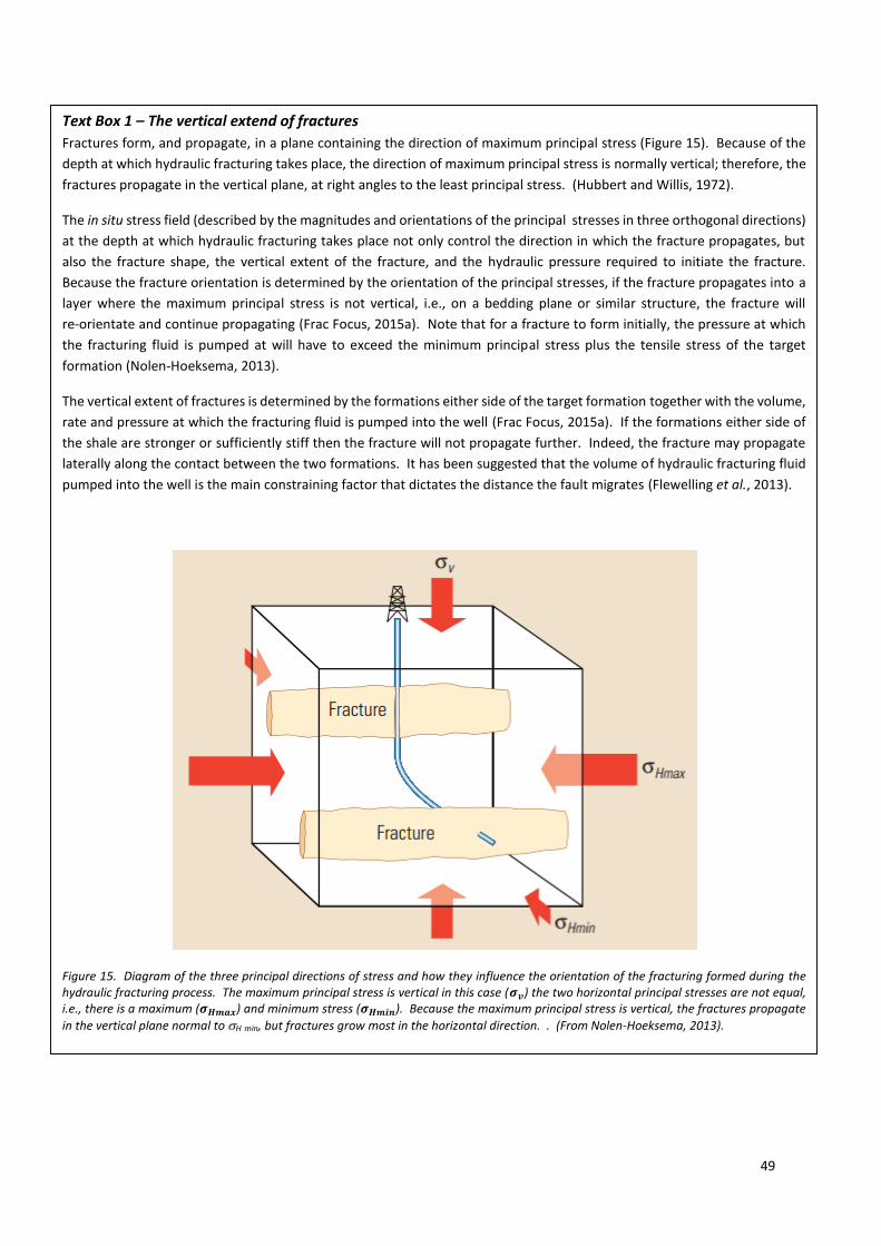
49
Text Box 1 – The vertical extend of fractures
Fractures form, and propagate, in a plane containing the direction of maximum principal stress (Figure 15). Because of the
depth at which hydraulic fracturing takes place, the direction of maximum principal stress is normally vertical; therefore, the
fractures propagate in the vertical plane, at right angles to the least principal stress. (Hubbert and Willis, 1972).
The in situ stress field (described by the magnitudes and orientations of the principal stresses in three orthogonal directions)
at the depth at which hydraulic fracturing takes place not only control the direction in which the fracture propagates, but
also the fracture shape, the vertical extent of the fracture, and the hydraulic pressure required to initiate the fracture.
Because the fracture orientation is determined by the orientation of the principal stresses, if the fracture propagates into a
layer where the maximum principal stress is not vertical, i.e., on a bedding plane or similar structure, the fracture will
re-orientate and continue propagating (Frac Focus, 2015a). Note that for a fracture to form initially, the pressure at which
the fracturing fluid is pumped at will have to exceed the minimum principal stress plus the tensile stress of the target
formation (Nolen-Hoeksema, 2013).
The vertical extent of fractures is determined by the formations either side of the target formation together with the volume,
rate and pressure at which the fracturing fluid is pumped into the well (Frac Focus, 2015a). If the formations either side of
the shale are stronger or sufficiently stiff then the fracture will not propagate further. Indeed, the fracture may propagate
laterally along the contact between the two formations. It has been suggested that the volume of hydraulic fracturing fluid
pumped into the well is the main constraining factor that dictates the distance the fault migrates (Flewelling et al., 2013).
Figure 15. Diagram of the three principal directions of stress and how they influence the orientation of the fracturing formed during the hydraulic fracturing process. The maximum principal stress is vertical in this case (𝝈𝒗) the two horizontal principal stresses are not equal, i.e., there is a maximum (𝝈𝑯𝒎𝒂𝒙) and minimum stress (𝝈𝑯𝒎𝒊𝒏). Because the maximum principal stress is vertical, the fractures propagate
in the vertical plane normal to H min, but fractures grow most in the horizontal direction. . (From Nolen-Hoeksema, 2013).
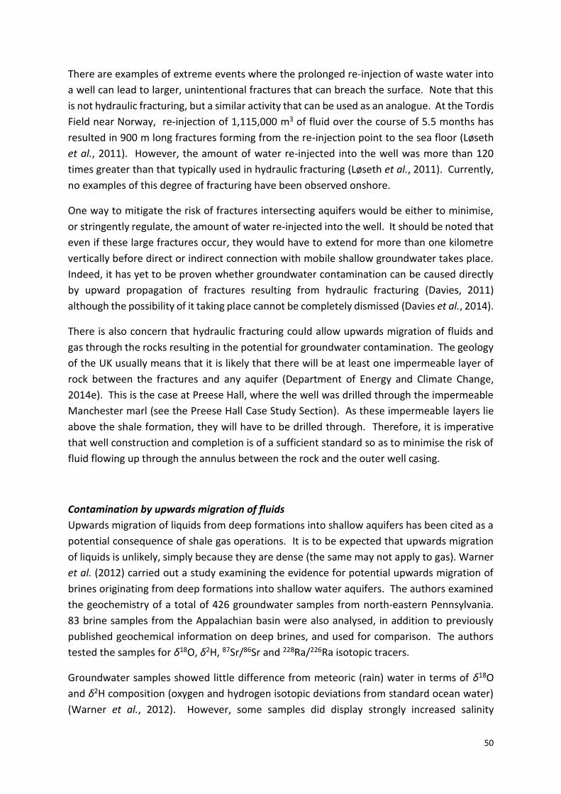
50
There are examples of extreme events where the prolonged re-injection of waste water into
a well can lead to larger, unintentional fractures that can breach the surface. Note that this
is not hydraulic fracturing, but a similar activity that can be used as an analogue. At the Tordis
Field near Norway, re-injection of 1,115,000 m3 of fluid over the course of 5.5 months has
resulted in 900 m long fractures forming from the re-injection point to the sea floor (Løseth
et al., 2011). However, the amount of water re-injected into the well was more than 120
times greater than that typically used in hydraulic fracturing (Løseth et al., 2011). Currently,
no examples of this degree of fracturing have been observed onshore.
One way to mitigate the risk of fractures intersecting aquifers would be either to minimise,
or stringently regulate, the amount of water re-injected into the well. It should be noted that
even if these large fractures occur, they would have to extend for more than one kilometre
vertically before direct or indirect connection with mobile shallow groundwater takes place.
Indeed, it has yet to be proven whether groundwater contamination can be caused directly
by upward propagation of fractures resulting from hydraulic fracturing (Davies, 2011)
although the possibility of it taking place cannot be completely dismissed (Davies et al., 2014).
There is also concern that hydraulic fracturing could allow upwards migration of fluids and
gas through the rocks resulting in the potential for groundwater contamination. The geology
of the UK usually means that it is likely that there will be at least one impermeable layer of
rock between the fractures and any aquifer (Department of Energy and Climate Change,
2014e). This is the case at Preese Hall, where the well was drilled through the impermeable
Manchester marl (see the Preese Hall Case Study Section). As these impermeable layers lie
above the shale formation, they will have to be drilled through. Therefore, it is imperative
that well construction and completion is of a sufficient standard so as to minimise the risk of
fluid flowing up through the annulus between the rock and the outer well casing.
Contamination by upwards migration of fluids
Upwards migration of liquids from deep formations into shallow aquifers has been cited as a
potential consequence of shale gas operations. It is to be expected that upwards migration
of liquids is unlikely, simply because they are dense (the same may not apply to gas). Warner
et al. (2012) carried out a study examining the evidence for potential upwards migration of
brines originating from deep formations into shallow water aquifers. The authors examined
the geochemistry of a total of 426 groundwater samples from north-eastern Pennsylvania.
83 brine samples from the Appalachian basin were also analysed, in addition to previously
published geochemical information on deep brines, and used for comparison. The authors
tested the samples for δ18O, δ2H, 87Sr/86Sr and 228Ra/226Ra isotopic tracers.
Groundwater samples showed little difference from meteoric (rain) water in terms of δ18O
and δ2H composition (oxygen and hydrogen isotopic deviations from standard ocean water)
(Warner et al., 2012). However, some samples did display strongly increased salinity

51
(Cl- >20 mg/L) which the authors attributed to brine migration along natural conductive
pathways, as there was no correlation between shale gas drilling activity and the location
from where these high salinity samples were taken. Although this study suggests overall that
the contamination of groundwater due to fluid migration from depth following from shale gas
activity is unlikely to take place, it does raise the point that these conductive pathways can
exist, and if brine can migrate upwards along them, then there is a chance that hydraulic
fracturing fluid and methane could do the same. The net result is that in areas in which
upwards migration of deep formation waters can take place there may be a greater risk of
shallow groundwater contamination (Warner et al., 2012). The authors suggest that future
research should include monitoring of areas of known upwards migration in order to establish
the source of the deep fluid, the connectivity of the pathways and the timescale over which
the upwards migration takes place.
The US National Energy Technology Laboratory (NETL) has recently published a study
examining hydraulic fracturing-related fracture growth and gas / fluid migration in Greene
Country, Pennsylvania (Hammack et al., 2014). The study involved monitoring seven wells
drilled into Upper Devonian / Lower Mississippian rocks overlying the fracturing area of six
horizontal Marcellus Shale wells (Figure 16); in addition, two vertical monitoring wells were
drilled into the Marcellus Shale. In order for migration of fracking and formation fluids to take
place, and hence for contamination of the groundwater to occur, the Tully Limestone (which
is considered to be the barrier that prevents fracture and fluid migration), located
approximately 85 m above the Marcellus Shale, would have to be penetrated by the fractures
and fluid (Figure 16) (Hammack et al., 2014).
Monitoring took place during and after hydraulic fracturing. Gas pressure and production
histories of three of the wells drilled into the Upper Devonian / Lower Mississippian rocks
showed no change in the 12 month period after fracturing ceased. This indicates that no
upwards migration of fluid took place, as a change in pressure would indicate communication
between the fluid / gas and the over-pressurised (meaning the gas pressure in the sale is very
high) shale (Hammack et al., 2014). Additional monitoring of possible background migration
of fluids took place two months before the fracturing took place. Measurements of gas and
produced water samples were taken from the seven wells drilled into the Upper
Devonian / Lower Mississippian rocks, as well as from the two vertical Marcellus Shale wells,
throughout the fracturing stages and for eight and five months respectively after fracturing
ended. Gas samples were examined for carbon (δ13CCH14) and hydrogen (δ2HCH4) isotope
signatures and produced water was tested for its strontium isotope composition. Clear
differentiation in terms of isotopic signatures can be seen between the two sets of wells
(Figure 17), thus indicating that no mixing, and hence no upwards migration, took place
(Hammack et al., 2014). The isotopic signatures also show little variation with respect to time
(Figure 17), this is also the case for the strontium isotope ratio of the produced water taken
from the Upper Devonian / Lower Mississippian wells (Figure 18) (Hammack et al., 2014).

52
Four perfluorocarbon tracers were also utilised during the fracturing stage of the operation
in order to establish whether upwards migration of fluids took place. The tracers were mixed
with hydraulic fracturing fluid and injected into a horizontal Marcellus Shale well at 10
fracturing stages. The introduction of the tracers took place after the well had been acidized
but before the proppant had been introduced into the hydraulic fracturing fluids. This
allowed the tracers to migrate to the most distant parts of the fractures. The tracers were
designed to form a non-aqueous, buoyant phase when entering the rock formations, thereby
facilitating easy upwards migration (Hammack et al., 2014). Tracers were found in the gas
samples taken from the Marcellus well into which the tracers were injected. Additionally,
tracers were found in an adjacent well, approximately 230 ft. from the tracer injection well.
The authors consider this to be a result of the perforation zones of each wellbeing in close
proximity to each other. Samples from the Upper Devonian / Lower Mississippian wells
nearest to the tracer injection well displayed no evidence of the presence of tracers during
the monitoring period of two months, therefore, suggesting that no upwards migration of
gas / fluid took place (Hammack et al., 2014).
Overall, the study found no evidence of upwards gas / fluid migration at any point in the
monitoring programme. Therefore, no evidence of groundwater contamination was found
resulting from fluid migration through the rock succession (Hammack et al., 2014). Continual
monthly (produced water) and bimonthly (gas) measurements are currently being made.
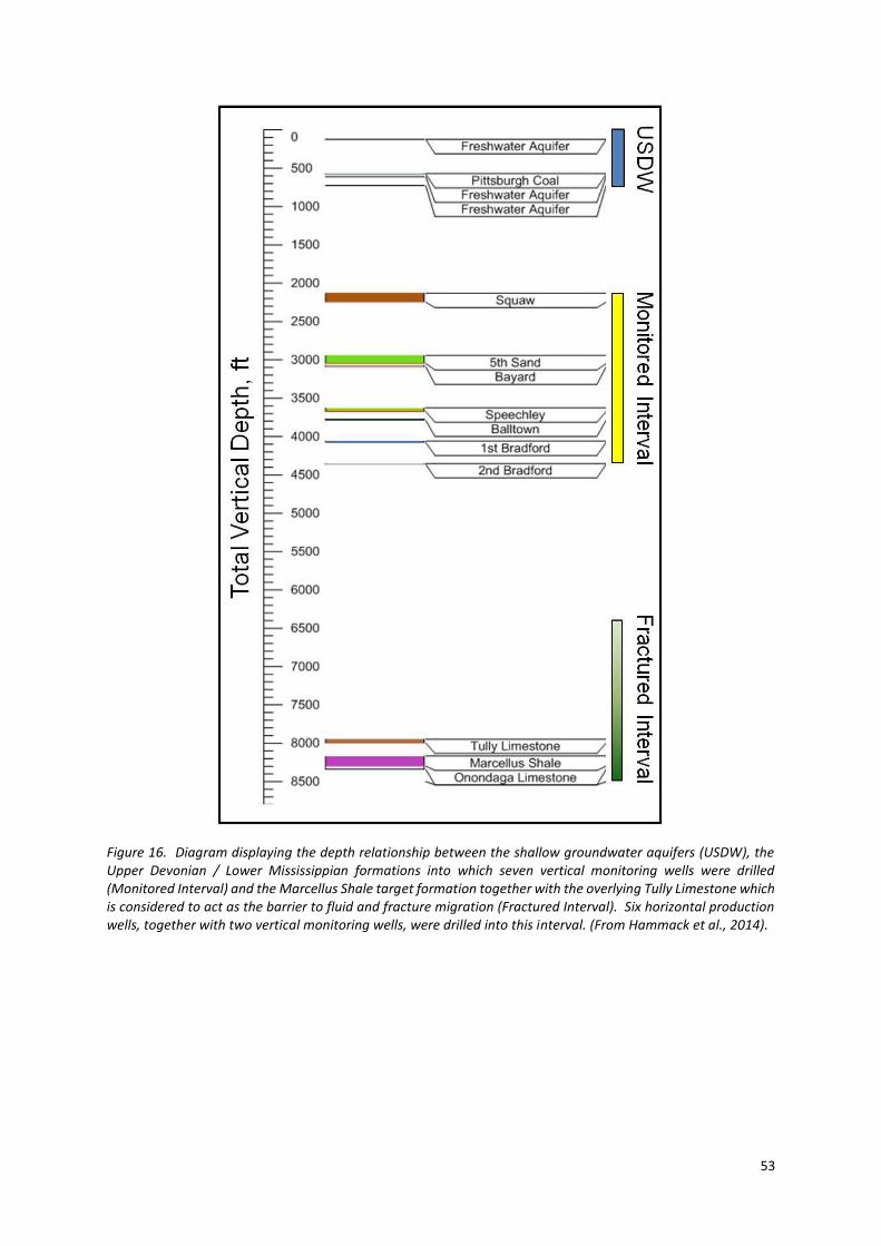
53
Figure 16. Diagram displaying the depth relationship between the shallow groundwater aquifers (USDW), the Upper Devonian / Lower Mississippian formations into which seven vertical monitoring wells were drilled (Monitored Interval) and the Marcellus Shale target formation together with the overlying Tully Limestone which is considered to act as the barrier to fluid and fracture migration (Fractured Interval). Six horizontal production wells, together with two vertical monitoring wells, were drilled into this interval. (From Hammack et al., 2014).

54
Figure 17. Top) Comparison between the isotope signatures of the Upper Devonian / Lower Mississippian monitoring wells and the vertical wells drilled directly into the Marcellus Shale. Note the clear differentiation between each group. Middle) Change in carbon isotope signature over the sampling period. UD-1-UD-7 denotes Upper Devonian / Lower Mississippian monitoring wells while MW-1 and MW-2 denote vertical Marcellus Shale wells. Bottom) Change in hydrogen isotope signature over the sampling period. The key for the middle and bottom plots are the same. Note that the levels in both the middle and bottom plot remain approximately

55
constant, Hammack et al. (2014) consider that the variation is within expected range. (From Hammack et al., 2014).
Figure 18. Plot of the change in strontium isotope ratio with time in five Upper Devonian / Lower Mississippian monitoring wells. Note the approximate consistency of the ratios both pre- and post-fracturing. (From Hammack et al., 2014).
A recent study aimed to model the potential for groundwater contamination by hydraulic
fracturing fluids through the use of pressure changes reported during gas well operation
(Myers, 2012). The study found that the changes in pressure associated with the process of
hydraulic fracturing could allow the upwards migration of fluids into aquifers in less than 10
years. However, as is a limitation of most modelling studies, simplifications must be made in
order to allow the model to be run (Vidic et al., 2013). These simplifications, although
necessary, limit the applicability of the results. In a comment on the study, Saiers and Barth
(2012) argued that key hydrological processes were neglected or misrepresented. For
instance, Myers (2012) assumed that the voids in the shale are filled only with water, whereas
in reality, the voids in the Marcellus and overlying formation contain both water and gas. The
result is that hydraulic conductivity could be orders of magnitude lower (Saiers and Barth,
2012; Vidic et al., 2013) as a result of capillary pressure effects. In order to understand fully
the potential for upwards migration of fluids over long timescales more such modelling
studies are required. However, it is likely that hydraulic conductivity will vary between drilling
sites, therefore, the results of such studies may be restricted in their applicability to other
shale gas operations.
56
Contamination by methane
Osborn et al. (2011) examined the methane content of aquifers (Catskill and Lockhaven
formations in Pennsylvania and the Genesee Group in New York) overlying the Marcellus and
Utica Shales in Pennsylvania and New York. 60 private drinking water wells were tested for
dissolved gas concentrations. The depths to which the wells were drilled, and hence where
the samples were taken from, varied between 36 to 190 m.
As a side note, the US Department of Interior has set limits on the permissible methane
content of groundwater. At levels of <10 mg/L of methane, the water is considered safe; at
levels of 10-28 mg/L, monitoring of the water supply is required. If the concentration rises
above 28 mg/L, i.e., the saturation point of methane in water at room temperature and
pressure, then immediate action is required to remediate the problem (Vengosh et al., 2014).
Osborn et al. (2011) found that methane was present in 51 of the 60 wells tested. However,
in areas around drinking water wells where more than one drilling site was located within
1 km the average methane content in drinking water was 19.2 mg CH4/L; the maximum
methane (supersaturated) content recorded was 64 mg CH4/L (Osborn et al., 2011). This
placed the average drinking water methane content within the hazard range set by the US
Office of Interior (10-28 mg CH4/L) and the maximum methane content well above the hazard
level (Osborn et al., 2011). The isotopic signature of ground water methane was found to
match that of a deep thermogenic source, i.e., the Marcellus and Utica Shales. Conversely, in
areas around drinking water wells with no active drilling sites within 1 km, the average
methane content was 1.1 mg CH4/L (Figure 19). In addition, the isotopic signature of this
methane indicated a biogenic or mixed biogenic and thermogenic source (Osborn et al.,
2011).
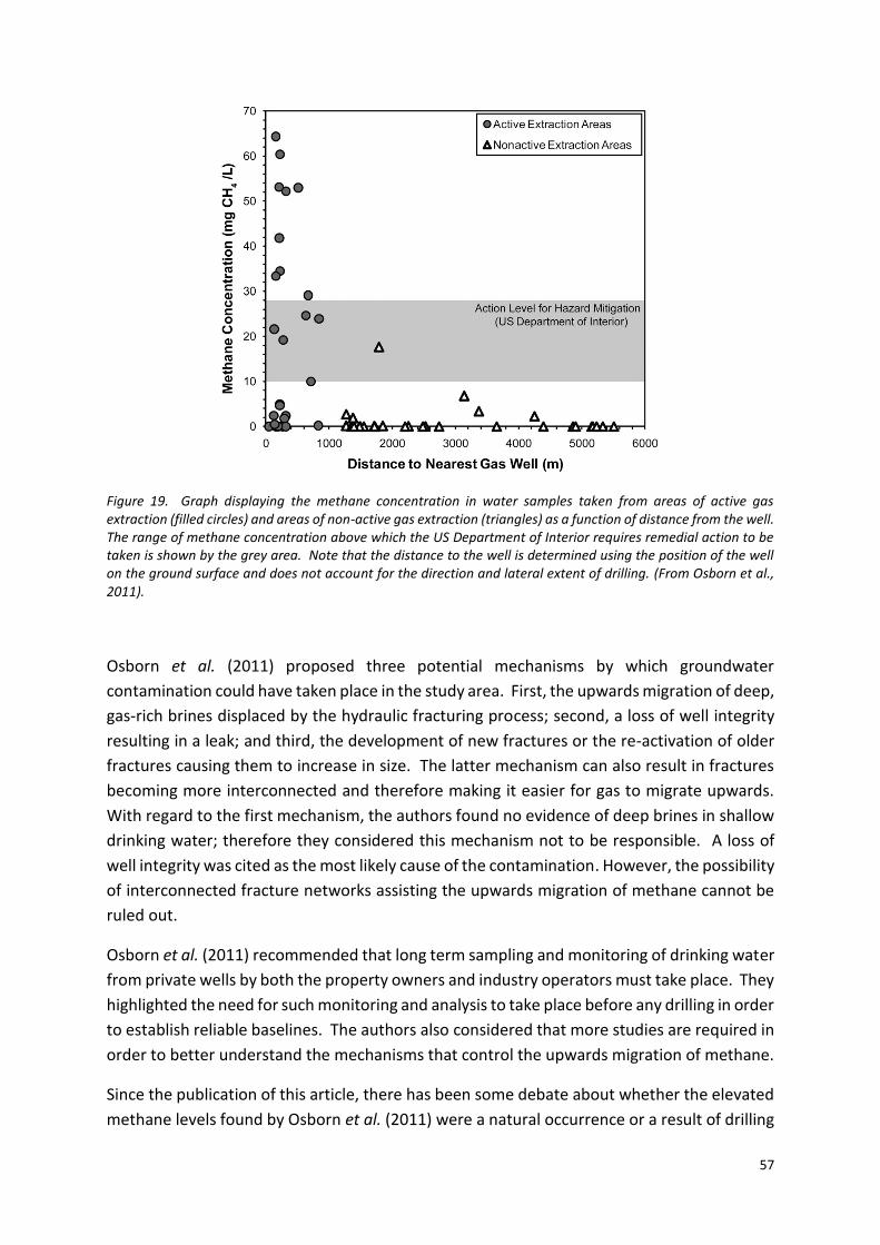
57
Figure 19. Graph displaying the methane concentration in water samples taken from areas of active gas extraction (filled circles) and areas of non-active gas extraction (triangles) as a function of distance from the well. The range of methane concentration above which the US Department of Interior requires remedial action to be taken is shown by the grey area. Note that the distance to the well is determined using the position of the well on the ground surface and does not account for the direction and lateral extent of drilling. (From Osborn et al., 2011).
Osborn et al. (2011) proposed three potential mechanisms by which groundwater
contamination could have taken place in the study area. First, the upwards migration of deep,
gas-rich brines displaced by the hydraulic fracturing process; second, a loss of well integrity
resulting in a leak; and third, the development of new fractures or the re-activation of older
fractures causing them to increase in size. The latter mechanism can also result in fractures
becoming more interconnected and therefore making it easier for gas to migrate upwards.
With regard to the first mechanism, the authors found no evidence of deep brines in shallow
drinking water; therefore they considered this mechanism not to be responsible. A loss of
well integrity was cited as the most likely cause of the contamination. However, the possibility
of interconnected fracture networks assisting the upwards migration of methane cannot be
ruled out.
Osborn et al. (2011) recommended that long term sampling and monitoring of drinking water
from private wells by both the property owners and industry operators must take place. They
highlighted the need for such monitoring and analysis to take place before any drilling in order
to establish reliable baselines. The authors also considered that more studies are required in
order to better understand the mechanisms that control the upwards migration of methane.
Since the publication of this article, there has been some debate about whether the elevated
methane levels found by Osborn et al. (2011) were a natural occurrence or a result of drilling
58
activity. This is due to the lack of previously determined baseline levels of methane from the
study area and the fact that the areas are known naturally to produce methane seeps of both
biogenic and thermogenic origin (Vidic et al., 2013). Biogenic gas is formed at shallow depths
and low temperatures by an anaerobic bacterial decomposition of sedimentary organic
matter. Thermogenic gas is formed at deeper depths by thermal cracking of sedimentary
organic matter into hydrocarbon liquids and gas, and thermal cracking of oil at high
temperatures into gas and pyrobitumen.
According to Vidic et al. (2013) the methane contents of groundwater found by Osborn et
al. (2011) were similar to those found by the US Geological Survey during a previous water
sampling survey which took place between 1997 and 2011 (Figure 20), suggesting that there
may have been pre-existing seeps. In order to provide an explanation for this, Vidic et al.
(2013) cited the fact that there have been approximately 350,000 oil and gas wells drilled in
Pennsylvania, the locations of approximately 250,000 of which are unknown. Therefore it may
be that these unknown wells are leaking and acting as conduits for upwards migration of
hydrocarbons. This emphasises the importance of baseline studies in the UK if shale gas
exploration and extraction are to go ahead.

59
Figure 20. A) Published values for methane in groundwater and the location of the respective sample sites. 239 sites sampled from 1999-2011 are in New York State, 40 sites sampled in 2005 are in Pennsylvania and 170 sites sampled from 1997-2005 in West Virginia. The lack of data points in Pennsylvania is due to Vidic et al. (2013) only including samples taken in 2005. B) Graph of the sample sites shown in A with arrows indicating the average methane content of the samples analysed by Osborn et al. (2011). (From Vidic et al., 2013).
Vidic et al. (2013) highlighted the fact that, at the time of publication, only one study had
compared the chemistry of groundwater before and after drilling (Boyer et al., 2012). The
60
study compared 48 water samples from drinking water wells over Pennsylvania in 2010 and
2011. It was found that no statistically significant difference existed between methane levels
before and shortly after drilling, nor was there any correlation between methane content of
water and distance from drilling sites (Boyer et al., 2012). It should be noted, however, that
this study was not peer reviewed. In addition, although no short term increases were seen,
because of the lack of studies on the timescales and mechanism of methane migration, it may
be that upwards migration of methane takes place over several years and would therefore
not be detected shortly after drilling had been completed. The study did find that the
methane concentration increased in a single water well shortly after well completion. The
authors attributed this to problems with well integrity resulting in a leak, they also noted that
this occurrence is consistent with the average rate of well integrity failure observed in the US
(approximately 3%) and is, therefore, to be expected (Boyer et al., 2012).
The frequency of methane detection in water wells varies considerably with respect to
geography. For instance, in the northeast of Pennsylvania, methane has been detected in 80-
85% of tested water wells (Molofsky et al., 2011; Osborn et al., 2011) whereas in the
southwest only 24% of tested water wells have had methane detected in the potable water
(Boyer et al., 2012). This could be attributed to the small sample size used by the Osborn et
al. (2011) or it could be that the geology in the northeast of Pennsylvania is more susceptible
to the upwards migration of methane (Warner et al., 2012; Vidic et al., 2013). On a wider
scale, these differences in geology could explain why there has been little in the way of
groundwater contamination problems in other shale gas producing areas in the US, i.e., the
Fayetteville shale in Arkansas (Vidic et al., 2013). Given that methane migration does occur
naturally, the above discussion further highlights the importance of baseline studies in areas
of potential shale gas exploration and extraction in the UK.
A more recent study by Darrah et al. (2014), building upon previous studies by Osborn et al.
(2011) and Jackson et al. (2013), examined water taken from drinking water wells in the
Marcellus and Barnett Shale areas known to have elevated methane levels. 113 samples were
taken from the Marcellus region and 20 from the Barnett region. The authors examined the
occurrence of the noble gas isotopes 4He, 20Ne and 36Ar, hydrocarbon (CH4, C2H6, C3H8 and N2)
and chloride (Cl-) contents of the water together with stable isotope compositions (δ13C-CH4
and δ13C2-CH6) and the elemental and isotropic compositions of the noble gases. The aim of
the study was to address two specific questions. First, is the methane found in drinking water
natural or of anthropogenic origin? Second, if fugitive methane contamination is taking place,
how is it happening?
Darrah et al. (2014) found that methane was present in water samples taken from wells in
the Marcellus Shale located >1 km from drilling sites; the methane was found in association
with elevated levels of natural brine components (i.e., He4 and Cl-). Water samples taken
from wells with nearby drilling sites (<1 km away) were either indistinguishable from those
taken from >1 km away, or displayed methane supersaturation together with low salt
61
concentrations. In the case of the samples with elevated natural brine components, the
authors considered these samples to represent natural migration of deep, gas-rich brines to
shallow depths. The methane-supersaturated samples also displayed high noble gas ratios
(i.e., CH4/36Ar and 4He/20Ne) which appear to be independent of Cl- concentration. This
indicates elevated thermogenic gas concentration.
Similar trends were found in samples taken from the Barnett Shale in 2012. Twelve water
wells were sampled, nine of which displayed noble gas ratios that suggested natural migration
of gas-rich brines. The remaining three had elevated CH4/36Ar and 4He/20Ne values,
suggesting anthropogenic contamination related to shale gas drilling and extraction. In order
to confirm the results, the authors re-sampled the twelve Barnett Shale drinking water wells
in 2013. An additional eight new wells were also sampled (total of 20 wells). The newly
sampled wells showed no indication of anthropogenic contamination. Ten of the original
twelve wells displayed minimal change, the remaining two displayed increased CH4/36Ar and 4He/20Ne values with no change in Cl-, in one case the values increased by an order of
magnitude. These results indicate that thermogenic gas, without accompanying brine,
contaminated these water wells in less than one year (Darrah et al., 2014).
The anthropogenically-contaminated water samples from the Marcellus Shale also displayed
decreased levels of 36Ar, 20Ne and N2 compared to non-contaminated samples. In the Barnett
Shale area, the three anthropogenically-contaminated wells sampled in the first sampling
instance also displayed decreased 36Ar, 20Ne and N2 values. The two wells which displayed
progressive contamination between the two sampling periods in 2012 and 2013 also
displayed decreasing 36Ar, 20Ne and N2 values. It should be noted that these decreases were
only seen in wells where the nearest shale gas site was <1 km away (Darrah et al., 2014). The
reduction in the concentration of these gases requires unique hydrogeological conditions.
Specifically, gas has to be introduced into the near-surface aquifer at a pressure of
>1 atmosphere, i.e., at a rate higher than natural groundwater flow (Darrah et al., 2014). The
authors argued that there is no obvious tectonic or hydraulic mechanism in either area that
would allow this to happen. This suggests that the mechanism of contamination was by well
integrity failure (Darrah et al., 2014).
Other evidence for methane contamination associated with shale gas activities comes in the
form of hydrocarbon molecular compositions (C2H6+/CH4) and stable isotope compositions
(δ13C-CH4). Elevated values for each of these are considered to be indicators of restricted
biogenic methane production (Darrah et al., 2014). Indeed, elevated levels were detected in
the samples considered to have undergone anthropogenic contamination by fugitive gas
(Darrah et al., 2014). In addition, the hydrocarbon composition levels of the gas in the
samples taken from the Marcellus Shale region match those of the gas extracted from the
drilling sites and that found in intermediate depth formations.
Darrah et al. (2014) concluded that samples that contained both methane and natural brine
components were the result of natural upwards migration of gas-rich brines. They

62
hypothesise that the natural upwards migration took place in three stages. First, sufficient
thermogenic methane formed in the shale source rock to allow the formation of a free gas
phase. This permitted the trace gases (e.g., 20Ne and 36Ar) to fractionate into the gas phase.
The degree of fractionation is dependent upon the partition coefficient of the gas in question.
In terms of the gases analysed by Darrah et al. (2014), He and Ne have higher partition
coefficients (i.e., lower solubility in fluids) compared with Ar and CH4, therefore, He and Ne
will preferentially fractionate into the gas phase. The next stage involves buoyant upwards
migration of the He and Ne enriched hydrocarbon phase. As this takes place, fractionation
continues to take place and the gas phase becomes progressively enriched with both Ne and
He as the other less soluble gases (Ar and CH4) re-dissolve into the water-saturated crust. The
overall result of this process is elevated 20Ne/36Ar and 4He/CH4 values in the gas phase. This
is observed in gases found at intermediate depth formations in the Marcellus Shale. The final
stage of migration involves the diffusion and equilibration of gases into shallow aquifers.
The groundwater samples considered to have experienced anthropogenic contamination due
to fugitive gas migration display significantly lower 20Ne/36Ar and 4He/CH4 values, suggesting
that migration took place with little fractionation, i.e., rapid upwards migration. The lack of
fractionation indicates that there was minimal interaction between the gas and the
intermediate formations, suggesting that either a failure in well integrity or an annular leak
was the cause. In order to differentiate between the two potential mechanisms, the
geochemical fingerprint was examined. Gas that originates from intermediate depth
formations, i.e., the gas that would be found in the aquifer if an annular leak had taken place,
has a lower δ13C-CH4 value than production gas. In addition, C2H6+/CH4 values are lower than
in production gas. When Darrah et al. (2014) examined these geochemical fingerprints, they
found three clusters of results in the Marcellus Shale and one cluster in the Barnett Shale
corresponded to gas found at intermediate depth formations. This suggests that poor
cementing likely resulted in an annular leak which, in turn, allow the rapid upwards migration
of gas. Four clusters corresponded to the composition of the Marcellus production gas,
indicating problems with well construction resulting in leaks of production gas in and around
the aquifer. One of these clusters exhibited evidence of significant fractionation during
migration from depth, resulting in drastically increased 20Ne/36Ar and 4He/CH4 values. The
authors attributed this to the “underground mechanical... failure” of a well prior to the
sampling taking place. The authors found no evidence of large-scale upwards migration of
gas caused by hydraulic fracturing.
Vengosh et al. (2014) suggested that the severity of any groundwater contamination could be
increased if oxidisation of fugitive methane takes place via bacterial sulphate reduction
reactions. When these reactions take place, they can act to mobilise other, more potentially
dangerous elements such as arsenic from the aquifer formation. The overall result is a further
decrease in water quality. Research to date has not produced conclusive evidence that this
takes place in areas associated with shale gas operations (Vengosh et al., 2014).

63
Another possible consequence of groundwater contamination by stray gas is the formation
of toxic trihalomethane compounds (Vengosh et al., 2014). These are compounds that form
in the presence of organic matter, in which halogen atoms substitute for the hydrogen atoms
in methane. Currently, there are no published studies that have observed these compounds
at shale gas sites. However, if both halogens and organic matter are present in the aquifer
after contamination has taken place then there is the potential for trihalomethane
compounds to form (Vengosh et al., 2014).
Contamination of surface water
Contamination of surface water by flowback fluid is also a potential hazard associated with
shale gas exploration and extraction. As discussed previously, when the hydraulic fracturing
fluid enters the rock formation of interest, it can leach chemical elements and compounds
from the rock. In addition, as discussed above, elevated salinity levels are also commonly
associated with the fluids produced in shale gas operations, and surface waters may become
more saline if a spill or leak occurs. These risks vary spatially as demonstrated in the US,
where the salinity of flowback fluids range from slightly less than that of seawater (total
dissolved salts = 25,000 mg/L), e.g., the Fayetteville Shale (25,000 mg/L), to well above
seawater, e.g., Marcellus Shale (180,000 mg/L) (Vengosh et al., 2014), note that the salinity
of seawater is 35,000 mg/L. It has also been shown that the chloride salinity and levels of
potentially dangerous elements, such as strontium and barium, vary naturally within rock
formations (Chapman et al., 2012; Barbot et al., 2013).
Vengosh et al. (2014) describe three main methods by which surface water contamination
can take place:
1. General leaks and spills of flowback fluid from on-site equipment, such as storage
tanks, pipework and open ponds.
2. Direct, unauthorised discharge of untreated flowback fluid into streams and other
surface water sources.
3. Inadequate treatment of flowback fluid, either on-site or in treatment plants, followed
by discharge into surface water sources.
The occurrence of surface water contamination events has been shown to increase in areas
of high density (>0.5 wells per km2) shale gas operations (Vengosh et al., 2014). Vengosh et
al. (2014) say that the risk of surface water contamination is increased in the instance of shale
gas operations, as gas production can rapidly decrease by as much as 85% within the first
three years of extraction. The result of this is that a sufficient number of wells needs to be
drilled in order to keep production at the required economic level. The more wells that are
drilled and fractured, the more risk there will be of a spill or leak taking place. Wells can also

64
be re-fractured in order to re-stimulate gas flow. This will involve more water being
transported on-site, increasing the risk of a spill or leak taking place.
Around conventional wells in Garfield County, Colorado, the percentage of private drinking
wells that had chloride concentrations higher than 250 mg/L increased from 4% in 2002 to 8%
in 2005 (Vengosh et al., 2014). These increases were associated with increasing thermogenic
methane (methane formed under high pressure and high temperature conditions, i.e., >1 km
below the Earth’s surface) in the groundwater, which, in turn, was associated with an increase
in the number of oil and gas wells in the county (Vengosh et al., 2014). The cause of the
increased salinity and methane content of the groundwater was attributed to leaks, either
from the well or from surface water storage pits (Vengosh et al., 2014). The authors say that,
if contamination were to take place at a shale gas site, the water chemistry of the
contaminated water source should be similar to that of the water in the target shale
formation or the water in intermediate depth formations. However, the authors also say that
there is currently no evidence of increased salinity of groundwater in shale gas sites in north-
eastern Pennsylvania that have experienced groundwater contamination via the infiltration
of stray gas. Hence salinity increase alone does not necessarily imply contamination from
shale gas production. More studies are therefore required in order to establish clearly the
extent of correlation between groundwater salinity and shale gas extraction.
There is documented evidence in the US of illegal disposal of untreated and inadequately
treated flowback fluid being released into surface waters, e.g. in the Acorn Fork Creek in
Kentucky (Papoulias and Velasco, 2013). The release of the fluid was considered to have
caused the death of local aquatic species, in addition to adversely affecting their general
health (Papoulias and Velasco, 2013). A study using the controlled release of hydraulic
fracturing fluids into a forest stream revealed that vegetation near to the stream was severely
affected by the contamination (Adams, 2011). In less than 10 days, vegetation had been
damaged or killed. Over the course of two years, over half of the trees within a 2 km2 area
around the stream were dead and the soil had been contaminated by sodium and chloride,
with the levels being 50-fold higher than before contamination (Adams, 2011). It should be
noted that this sort of disposal is against the law in the UK. Therefore, as long as the law is
followed by the operator, the risk of surface water contamination through deliberate release
should be minimal.
Inadequate treatment of flowback fluid before being discharged into surface waters can result
in contamination. It has been demonstrated by Warner et al. (2013) that treated flowback
water discharged from water treatment sites in Pennsylvania still contained elevated salinity,
naturally occurring radioactive materials (NORM), toxic metals and volatile organic
compounds (VOCs), such as benzene, after treatment. VOCs are organic compounds that
have a high vapour pressure, and therefore low boiling point. They have been cited as a
potential human health risk arising from shale gas exploration and extraction (Bunch et al.,
2014). VOCs are found within many everyday products including paints, disinfectants,

65
cosmetics, glues and pesticides (United States Environmental Protection Agency, 2012). A
report by the New York State Department of Health (2014) found that VOCs can increase the
odour in the local atmosphere; they can also increase the chance of respiratory problems.
VOC emissions can be managed using green completions in the same way as fugitive methane
emissions. In terms of salinity, the concentration of chloride and bromide in the treated fluid
were 80,542 mg/L and 644 mg/L respectively at the point of discharge compared to
background levels (18 mg/L and 0.05 mg/L respectively) present upstream (Warner et al.,
2013). In terms of salinity, the flowback fluid was 2.3 times the salinity of seawater. As far as
2 km downstream from the discharge point, levels of bromide were found to be 16-fold higher
than background levels (Warner et al., 2013).
Bromide poses a potentially significant hazard as its presence can result in the formation of
carcinogenic trihalomethanes in chlorinated drinking water (e.g., Chowdhury et al., 2010a, b).
Evidence from tests on drinking water in some areas of Pennsylvania, specifically the
Monongahela River and Pittsburgh, have shown elevated levels of bromide related
trihalomethanes related to the improper treatment of waste fluids (States et al., 2013; Wilson
and Van Briesen, 2013). If the flowback fluid is transported to off-site facilities for treatment
then it is possible that this lack of appropriate treatment is not the fault of the operator, but
more the fault of either the authorities that decide which water treatment facilities are able
to treat properly the fluid, or the companies who operate the facilities. If shale gas
exploration and extraction goes ahead in the UK, the inspection of the procedures in
operation at these water treatment plants will be important in order to minimise the surface
water contamination hazard. Vengosh et al. (2014) point out that bromide related
trihalomethane can also form in wastewaters associated with other forms of industrial
activity, such as conventional oil and gas operations. On account of this, they recommend
continuing research in order assess to more fully the potential for surface water
contamination from waste waters arising from shale gas operations.
Vengosh et al. (2014) point out that “over time, metals, salts, and organics may build up in
sediments, scales, and soil near wastewater disposal and/or spill sites. Each respective
compound has a given solubility and reactivity (e.g., adsorption), the latter commonly
described by the distribution coefficient (Kd) that varies as a function of pH, Eh, temperature,
and the occurrence of other components in the water. As a result, the physicochemical
conditions of surface waters and the distribution coefficients of each compound will
determine how it interacts with particulate matter (e.g., colloidal particles) or river sediments.
Ultimately, these properties will determine the long-term environmental fate of such reactive
contaminants; reactive constituents would be adsorbed onto soil, stream, or pond sediments
and potentially pose long-term environmental and health risks.”
There is evidence for contamination of sediments located downstream of water treatment
plants in Pennsylvania (Warner et al., 2013). The NORM levels, specifically radium isotopes
(228Ra/226Ra), in these sediments matched those of brines originating from the Marcellus

66
Shale, therefore indicating that there is a direct relation between contamination and shale
gas waste water (Warner et al., 2013). In one instance, the levels of NORM in sediments at
one treatment facility exceeded safe levels for disposal of radioactive material (Warner et al.,
2013). This is potentially significant as the fluid treated at this facility was likely dealt with
using the appropriate procedures, yet elevated levels of contaminants still built up over time.
The UK should be aware of this if shale gas exploration and extraction proceeds. Techniques
for long term monitoring of discharge locations should also be considered.
Groundwater contamination in the UK
Past instances of groundwater contamination in the UK have come from abandoned coal
mines (Younger et al., 2002). Although now-abandoned coal mines were continually drained
whilst in operation, after decommissioning, drainage was stopped. After 10-20 years,
groundwater rebound can take place, resulting in the aquifer becoming contaminated by
saline fluids of deeper origin than could have become acidified by reaction with pyrite, and
can carry large amounts of colloidal iron oxide (the acid-mine-drainage problem). This series
of events took place in the Durham Coalfield where a public water supply was contaminated,
and consequently failed to meet EU groundwater quality standards (Neymeyer et al., 2007).
Abandoned coal mines can also result in the release of methane; in 2008 UK coal mines were
estimated to have produced approximately 14 million m3 of methane (Davies et al., 2014).
In order to minimise the risk of groundwater contamination, environmental regulations have
been put in place that control the design, construction, operation and monitoring of the well
and associated activities. Part of the planning application process is the submission of a
hydrogeological report to the EA. The report details the presence of any ground or surface
water as well as the measures proposed to mitigate any risks to the environment from all
stages of shale gas operations. This requires inclusion of details about the methods used to
construct the well, and the monitoring processes in place to monitor the well integrity.
Additionally, the report must state the composition of the hydraulic fracturing fluid itself, the
presence of any NORM in the local geology, how the water needed for the fracturing fluid is
to be acquired and how the waste from the site will be managed (Department of Energy and
Climate Change, 2014e).
As has been discussed previously, there have been examples of well integrity failure in the US
which has resulted in groundwater contamination (Darrah et al., 2014). It should be noted
that cases of groundwater containing elevated levels of methane have been attributed to
failures in the construction of the well, not to the propagation of a fractures that introduce
pathways to the shallow overlying aquifer (Darrah et al., 2014; Vengosh et al., 2014). It is
considered that if best practices are followed in the UK, the risks of such well-failures should
be minimal. Best practices are outlined by the United Kingdom Onshore Oil and Gas
Operators Group (UKOOG) and DECC (Department of Energy and Climate Change, 2013;
United Kingdom Onshore Operators Group, 2015).
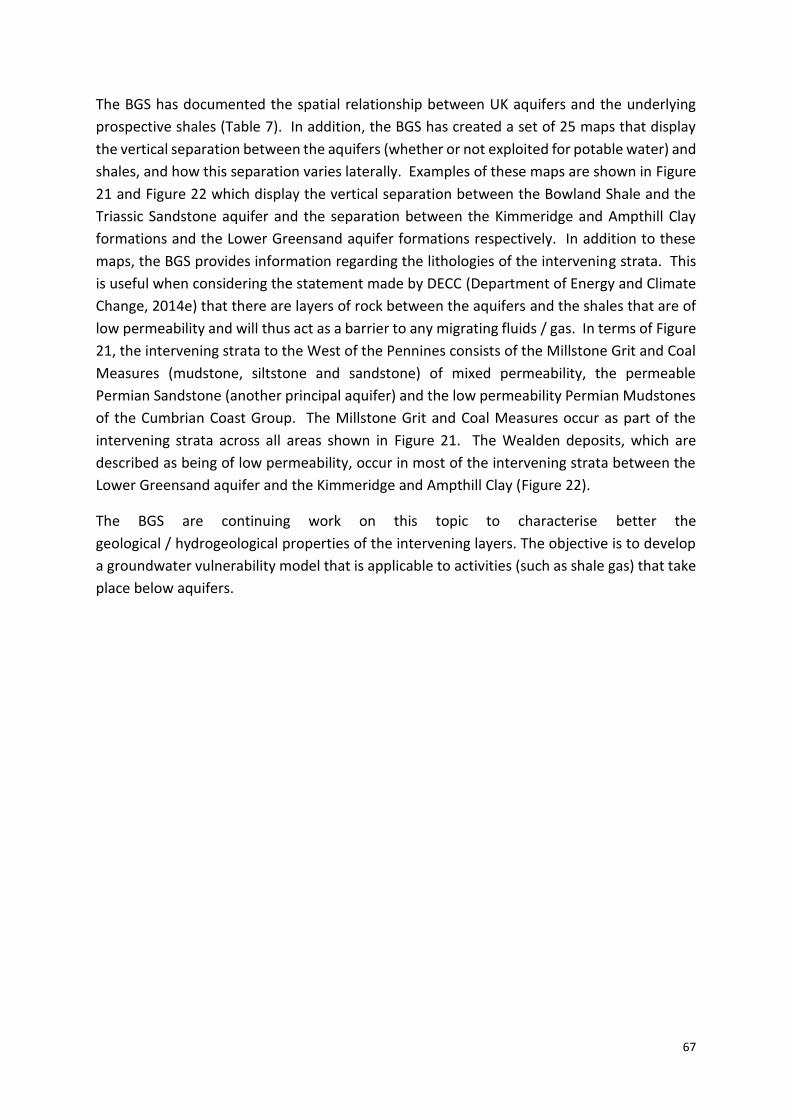
67
The BGS has documented the spatial relationship between UK aquifers and the underlying
prospective shales (Table 7). In addition, the BGS has created a set of 25 maps that display
the vertical separation between the aquifers (whether or not exploited for potable water) and
shales, and how this separation varies laterally. Examples of these maps are shown in Figure
21 and Figure 22 which display the vertical separation between the Bowland Shale and the
Triassic Sandstone aquifer and the separation between the Kimmeridge and Ampthill Clay
formations and the Lower Greensand aquifer formations respectively. In addition to these
maps, the BGS provides information regarding the lithologies of the intervening strata. This
is useful when considering the statement made by DECC (Department of Energy and Climate
Change, 2014e) that there are layers of rock between the aquifers and the shales that are of
low permeability and will thus act as a barrier to any migrating fluids / gas. In terms of Figure
21, the intervening strata to the West of the Pennines consists of the Millstone Grit and Coal
Measures (mudstone, siltstone and sandstone) of mixed permeability, the permeable
Permian Sandstone (another principal aquifer) and the low permeability Permian Mudstones
of the Cumbrian Coast Group. The Millstone Grit and Coal Measures occur as part of the
intervening strata across all areas shown in Figure 21. The Wealden deposits, which are
described as being of low permeability, occur in most of the intervening strata between the
Lower Greensand aquifer and the Kimmeridge and Ampthill Clay (Figure 22).
The BGS are continuing work on this topic to characterise better the
geological / hydrogeological properties of the intervening layers. The objective is to develop
a groundwater vulnerability model that is applicable to activities (such as shale gas) that take
place below aquifers.
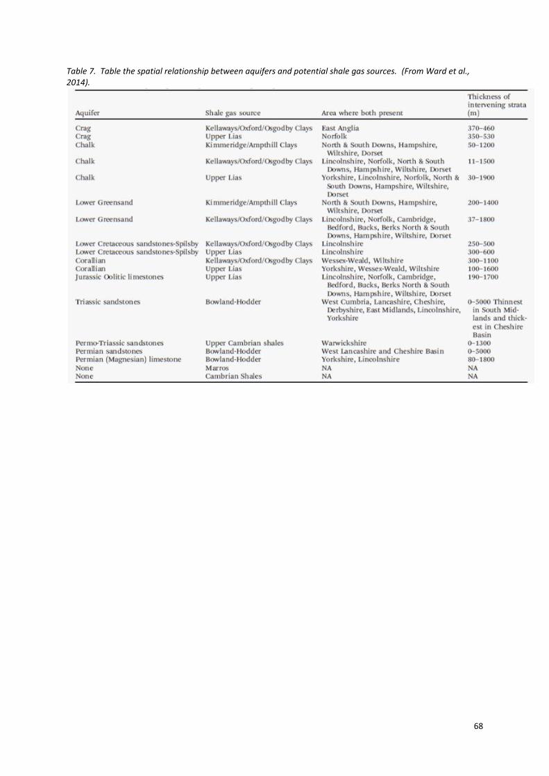
68
Table 7. Table the spatial relationship between aquifers and potential shale gas sources. (From Ward et al., 2014).

69
Figure 21. Map displaying the lateral variation in intervening strata thickness between the Triassic Sandstone aquifer and the Bowland shale. (From British Geological Survey, 2015b).

70
Figure 22. Map displaying the lateral variation in intervening strata thickness between the Lower Greensands aquifer and the Kimmeridge and Ampthill Clays. (From British Geological Survey, 2015a)
71
Well abandonment
Many of the same concerns outlined in the well integrity section also apply to well
abandonment. The issue of fluid leakage and fugitive gas emissions will likely become more
important during, and in the time after, well abandonment. During exploration and
extraction, constant monitoring of the well takes place. However, after the well has been
abandoned, it is likely that the frequency with which the well is monitored will decrease. As
time goes on, the risk to the environment potentially increases as cement can undergo
degradation; the casing can also fracture and corrode at the connections between sections
(Davies et al., 2014; Jackson, 2014). Degradation of the cement can result increased
permeability, thus introducing a potential pathway for fluid flow (Davies et al., 2014).
Once all operations at the site have ceased, it is the responsibility of the operator to ensure
that the site is restored to a state similar to that prior to the drilling, or to a condition that
would allow it to be re-visited at a later date (Department of Energy and Climate Change,
2014b). In order for the well to be suitably abandoned, the well must be securely sealed so
that there can be no leakage from within the well bore. In order to seal the well, cement is
pumped into the production casing and a steel cap is fitted to the top of the well (Davies et
al., 2014). A typical abandoned conventional oil / gas well can be seen in Figure 23. Note that
multiple cement plugs are used, one at the depth at which perforation takes place, i.e., the
production zone, and one at aquifer depth. The top of the production zone plug extends into
the caprock formation. This is done in order to ensure complete isolation between the
production zone and the well (Choi et al., 2013).

72
Figure 23. Schematic diagram of an abandoned conventional oil and gas well. (From Choi et al., 2013).
UKOOG has published industry guidelines related to all stages of well development, appraisal
and abandonment (United Kingdom Onshore Operators Group, 2015). UKOOG say that
operators should conform to the Oil and Gas UK Suspension and Abandonment Guidelines.
They also suggest that operators should consider the following factors when planning well
abandonment (United Kingdom Onshore Operators Group, 2015):
Height of the cement in annulus outside casing
Any permeable zones that should be cemented
Areas of cementing casing overlaps
Cement abandonment plugs need to cover the entire diameter of the well. Down-
hole equipment, e.g., cables, should be removed from the well
The type of fluid in the annuli above the cement.
The process of injecting cement into the annulus is more difficult than primary
cementing.
The process of well decommissioning and abandonment has been outlined by the EA
(Environment Agency, 2012a). The EA says that, in order for a well or borehole to be
abandoned in a satisfactory manner, it must be made safe, structurally sound and backfilled.
73
All these measures are to prevent the unplanned release of hydrocarbon and the upwards
migration of fluids into shallow groundwater areas (Environment Agency, 2012a, b). The EA
also differentiates between well abandonment and well suspension. Suspended wells are
those that are temporarily abandoned during parts of the well lifecycle while abandoned wells
cannot be used again (Environment Agency, 2012b). If a well is suspended, it must be
maintained in such a state that a routine work over could restore it to regular operation
(Environment Agency, 2012b).
When the decision to abandon a well is made, both DECC and the Health and Safety Executive
(HSE) have to be notified. The operator must submit an abandonment application to DECC
which must be approved before any work can proceed. This contains information regarding
the specifications of the abandoned well together with an abandonment plan (Environment
Agency, 2012b). Once approved, the HSE must be given at least 21 days’ notice before
abandonment begins (Environment Agency, 2012b).
OGUK, the trade body that represents the UK offshore hydrocarbon industry, published
guidelines on well integrity throughout the lifecycle of extraction operations in 2009 (Oil and
Gas UK, 2009). The EA uses these guidelines, in conjunction with the American Petroleum
Institute’s (API) recommended practice guidelines on environmental protection during
onshore operations (American Petroleum Institute, 2009), to inform the approach that should
be taken with UK onshore shale gas operations. However, the EA’s review of casing
installation at shale gas sites (Environment Agency, 2012b) summarises the relevant
guidelines for well abandonment made in both the OGUK and API reports. These are
summarized below (Environment Agency, 2012b):
All distinct permeable zones (group of zones originally at the same pressure regime
between which fluids can flow) through which the well passes must be isolated from
the surface, and from each other, by at least one permanent barrier (i.e., a cement
plug). The barrier must provide a permanent seal and extend across the entire cross-
section of the well.
An additional barrier should be installed at the base of any groundwater formations.
This is designed to prevent contamination of groundwater in addition to protecting
surface waters and soils from any fluids within the well. Many US States require
barriers to be installed at the base of the surface casing and / or between each
production zone.
If the permeable zone is hydrocarbon bearing then two barriers are required, although
these can be combined into a single large barrier covering the entire vertical extent of
the hydrocarbon bearing zone.
In the case where multiple hydrocarbon bearing zones are in close vertical proximity
to each other, the lower barrier for the upper zone can act as the upper barrier for the
lower zone.
74
Cement is the material most commonly used to form the barriers. Other materials
can be used although they must have certain properties, i.e., permeability, integrity,
non-shrinkage, ductility versus brittleness, chemical resistance and bonding capacity.
Permanent barriers are recommended to be at least 30 m in length; however, a barrier
length of 150 m should be used where possible.
If permeable zones are <30 m apart, it is recommended that the gap between the
zones be completely bridged with a cement column. The top of the upper section of
the barrier should extend >30 m above the highest potential flow point.
In the situation where two barriers are combined into one, the total length should be
>60 m. More typically, a barrier length of 250 m is used. The top of the barrier should
extend 60 m above the highest potential flow point.
The integrity of the annulus directly adjacent to the cement plug must be ensured in
order to form a complete seal. The original cement and casing of the well are not
considered to be permanent barriers as they can corrode or degrade with time. If
problems with the cement or casing are detected prior to the installation of the
barriers, remedial action must be taken. Such action can include perforating the
casing and pumping cement slurry through the perforations (cement squeeze) or
milling away casing and / or cement and replacing the removed material with cement.
Permanent barriers, once installed, must be tested and verified in order to ensure that
they are in the correct location and form an adequate seal with the well casing.
If a zone of irretrievable radioactive material is found, a permanent barrier should be
installed and the zone sealed off. These areas should also be surveyed, tagged and
reported to the appropriate authority.
Removal of downhole equipment is not required as long as the seal formed by the
installed barrier is sufficient and zonal isolation is achieved. However, wires and / or
cables should not form part of the barrier as they can act of potential flow paths.
If well completion casing, e.g., production casing, cannot be removed from the well,
extra precautions must be made to ensure that the barriers around such areas are
sufficient and that the performance of the barriers is verified.
Barriers installed in wells with significant concentrations of acidic compounds, e.g.,
CO2 and H2S, the barriers should be designed to withstand corrosion from such
compounds.
Potentially harmful or polluting fluids, e.g., mud and hydrocarbons, found above the
uppermost barrier should be removed as much as is reasonably possible. A cement
plug should then be installed at / near to the ground surface to prevent runoff entering
the well.
Finally, the casing should be cut-off below the ground surface. A casing stub (plate)
should then be welded onto the top of the well. The well cellar should then be filled
with a suitable material and surface condition restored to a level close to that prior to
drilling.
75
The EA also outline problems that can occur during, and after, well abandonment. The two
main challenges are the inability to remove down-hole equipment, the method of dealing
with this is outlined above, and the failure to create adequate seals (Environment Agency,
2012b). The main problem that could potentially be encountered after abandonment is
corrosion resulting in the connection between flowing zones (Environment Agency, 2012b).
Once a well has been abandoned to a satisfactory degree, the responsibility of aftercare and
monitoring lies with the operator (United Kingdom Onshore Operators Group, 2015).
From the research carried out for this report, there appears to be no provisions or legislation
in place regarding what happens to abandoned decommissioned and abandoned wells if the
operator goes out of business. This is a severe shortcoming in the current legislation that will
need to be addressed if shale gas exploration and extraction is to go ahead in the UK.
Currently, there is little in the way of monitoring of abandoned wells in the UK (Davies et al.,
2014). These same authors proposed that the wells should be inspected 2-3 months after the
cement plugs have been inserted into the well. Inspection should cover gas migration and
casing pressure. Inspection frequency can then be reduced providing that there is no
evidence of the well leaking; the well can then be cut off and buried. Any further inspection
should focus on soil monitoring, at a recommended interval of once every five years (Davies
et al., 2014) or if there is cause to think that well integrity might be compromised, e.g., a
seismic event. DECC, together with industry operators, are currently putting in place rules to
ensure that monitoring and restoration are maintained at abandoned sites, even if the
operator goes out of business (Department of Energy and Climate Change, 2014b).
76
Waste residues
During the drilling of the well, cuttings are produced and must be disposed of in an
environmentally friendly manner. The most common methods of disposing of the drill
cuttings is either transport to hazardous or non-hazardous landfill site, depending on the
concentration of salt and other chemicals, or spreading on agricultural land, both of which
are normally permitted by the EA (Stamford and Azapagic, 2014). However, spreading onto
agricultural land is not normally carried out in the UK. Some of the waste may be
contaminated, either by material dissolved from the shale, from the fluid base (i.e., oil) or
from chemicals in the fluid. In this case the method of disposal will need more careful
consideration. Stamford and Azapagic (2014) suggested that in the average well, 60% will be
spread on agricultural land while the remaining 40% will be disposed of in landfill. In the best
case scenario, 100% would be deposited in landfill, while in the worst case, all the waste will
be spread over agricultural land.
The main form of waste resulting from hydraulic fracturing is the water that returns to the
surface after fracturing has taken place, i.e., flowback fluid. 20-40% of the fluid injected into
the well returns to the surface as flowback following the fracturing stage, the majority of the
remaining fluid returns to the surface over time (Cuadrilla Resources Ltd., 2015). Note that
the fluid returns through the well, not the surrounding rock. Approximately 80% of the fluid
introduced to the well returns to the surface (note this is inclusive of the 20-40% that returns
during the fracturing stage), the remainder remains in the fractured rock. Due to the lack of
data on hydraulic fracturing of shale in the UK and the variability of local geology, it is difficult
to say how much of the fluid will return to the ground surface (Stamford and Azapagic, 2014).
As discussed previously, once these fluids have returned to the surface, there is a risk of
surface contamination if a spillage occurs. This is particularly the case in the US where open
pit storage is commonly used to store flowback fluid. In order to prevent any surface
contamination, UK regulation dictates that the fluid must be safely stored in robust covered
steel tanks before being treated and disposed of (Department of Energy and Climate Change,
2014e). This is done in order to minimise any emissions to the atmosphere and reduce the
risk of spillage. The drilling site must also be designed so that any spillage is avoided. It should
be noted that the use of tanks does not eliminate emissions as, as the tanks fill up, air and
hydrocarbon VOCs are vented to the atmosphere. In order to minimise emissions, Green
Completions are used. This allows gas that would be vented is either safely flared or captured
and sold (see Mitigating and controlling emissions section for more details regarding green
completions). In the US, the use of green completions is now mandatory during the
production stage but not for the exploration and appraisal stages. If a spill does take place,
measures must be taken to contain the spill and minimise the environmental impact.
The flowback fluid itself is classified by DECC as mining waste and, as such, needs to be
disposed of in accordance to the mining waste regulations put in place by the relevant
national EA. In addition, a plan for waste management based on laboratory tests must be in

77
place before drilling begins. During the operation of the site, the relevant authorities must
be informed before any movement of waste takes place (Department of Energy and Climate
Change, 2014e).
There are a number of methods by which flowback can be suitably disposed. One such
method is on-site recycling where the flowback is treated and the water re-used in the
fracturing process (Rassenfoss, 2011). The remaining material that cannot be recycled is
transported to a waste treatment facility. Another method is simply to transport all of the
waste from the site to an external treatment and disposal facility. Lastly, the waste material
can be fed into a special sewer designed to handle waste water. This method requires special
permission from the local utilities company (Department of Energy and Climate Change,
2014e).
The radioactive elements brought back to the surface in flowback fluid pose a potential hazard
to the site employees if the concentration of NORM is high or if prolonged exposure occurs
(Environment Agency, 2013). The way of dealing with the NORM brought up to the surface is
dependent upon the concentration or activity in the flowback. If the concentration is above
thresholds previously defined by the EA, a radioactive substances licence is required, whereas
if the concentration is below the threshold, the waste will be disposed according to those
defined by mining waste regulations. As with flowback disposal, the operator must submit a
plan for the disposal of the NORM contaminated material that includes details about the
handling and disposal process, in addition to the measures in place to mitigate the risk to
people and the environment (Department of Energy and Climate Change, 2014e).
At the Preese Hall site, Cuadrilla stored all of their wastewater in double-skinned steel tanks
(Environment Agency, 2011; Cuadrilla Resources Ltd, 2015). Both Cuadrilla and the EA carried
out regular tests on the wastewater; note that the EA can also carryout unannounced tests.
Once the water was ready for disposal, the wastewater was transported to a water treatment
plant in Davyhulme (Environment Agency, 2011; Cuadrilla Resources Ltd, 2015). This
treatment plant currently treats wastewater from other industrial sources and has the
capability to deal with the contaminants within the wastewater (Environment Agency, 2011).
Before treatment, the water is tested by the treatment plant (Cuadrilla Resources Ltd, 2015).
Once treated, the Davyhulme plant is permitted to discharge the water into the Manchester
Ship Canal (Environment Agency, 2011). A general overview of the water treatment process
in the UK can be seen in Figure 24.
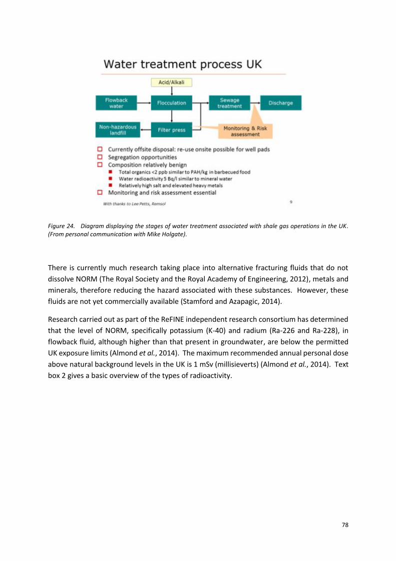
78
Figure 24. Diagram displaying the stages of water treatment associated with shale gas operations in the UK. (From personal communication with Mike Holgate).
There is currently much research taking place into alternative fracturing fluids that do not
dissolve NORM (The Royal Society and the Royal Academy of Engineering, 2012), metals and
minerals, therefore reducing the hazard associated with these substances. However, these
fluids are not yet commercially available (Stamford and Azapagic, 2014).
Research carried out as part of the ReFINE independent research consortium has determined
that the level of NORM, specifically potassium (K-40) and radium (Ra-226 and Ra-228), in
flowback fluid, although higher than that present in groundwater, are below the permitted
UK exposure limits (Almond et al., 2014). The maximum recommended annual personal dose
above natural background levels in the UK is 1 mSv (millisieverts) (Almond et al., 2014). Text
box 2 gives a basic overview of the types of radioactivity.
79
The Almond et al. (2014) study analysed the flowback fluid expelled from the Carboniferous
Barnett Shale (US), the Carboniferous Bowland Shale (UK), and the Silurian Shales of Poland.
To provide a reference for the concentration of NORM in flowback fluid, groundwater from
the basins containing each of the three shales was also analysed, as were surface water
sources, i.e., reservoirs. Background levels of both radium species measured in groundwater
Text box 2 – Types of radioactivity
There are three different types of radiation, i.e., alpha, beta and gamma. Each type of radiation can travel
different differences and can penetrate different materials.
Alpha particles are simply protons, and examples of alpha particle emitters are thorium-232, radon-222,
uranium-238 and radium-226. The latter two are present in varying amount in nearly all rocks, soils and
water (US Environmental Protection Agency, 2012). The particles travel a few centimetres from their source
and can be stopped by a piece of paper or clothing, therefore, in order for human exposure to occur, alpha
particles must be ingested (Classic, 2013). If inhaled, alpha particles have been shown to cause lung cancer
(US Environmental Protection Agency, 2012).
Beta particles are simply electrons and can travel short distances up to 1 m and is moderately penetrating,
however, particles can be stopped by a 3 mm piece of aluminium but can penetrate clothing and skin down
to the level where new skin cells are produced (the germinal layer) (Classic, 2013) If prolonged skin exposure
to high levels of beta-emitting materials takes place there is the potential to cause skin injury. Examples of
beta emitters are strontium-90, carbon-14, sulphur-35 and radium-228. The latter of which can be harmful
if ingested (Sperger et al., 2012; Classic, 2013).
Gamma radiation is a form of electromagnetic radiation similar to X-rays but are of comparatively higher
energy, higher frequency and shorter wavelength (Classic, 2013). They are also the most energetic type of
radiation depending on the intensity of the source, can require several inches of dense material, e.g., lead
or metres of cement to absorb the waves. This means that gamma rays can travel through the body,
therefore making them the most dangerous of the three types of radiation (Classic, 2013). Some examples
of gamma emitters are iodine-131 and radium-226. .
Radiation is measured in either grays (Gy) or sieverts (Sv) for absorbed and equivalent dose respectively.
Note that these units differ from Becquerels (Bq) which are a measure of radioactivity given in terms of the
number of decays per second.
Many radioactive elements occur naturally as part of rocks the in the Earth’s crust, e.g., uranium, radon and
potassium, as such, they are included in the NORM umbrella term (Sperger et al., 2012). Rocks, including
shale, contain some of these radioactive elements. For instance, the Marcellus Shale contains naturally
occurring uranium and thorium and their radioactive decay products, e.g., radium-226 (Sperger et al., 2012).
Because rocks contain radioactive elements, the risk these pose will depend on the elements in the rock and
their concentrations, and hence the type and amount of radiation emitted.
The concentration of uranium within shale may mean that it emits 20 times the background level of
radiation, although this still a tiny amount. Because of this, gas-bearing shale deposits have been located
based on detected gamma radiation levels (Resnikoff et al., 2010). The detection of gamma radiation is also
used to detect the total organic carbon (TOC) content of shales beneath the ground surface.
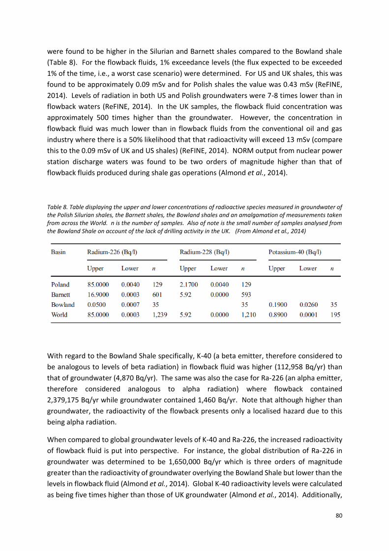
80
were found to be higher in the Silurian and Barnett shales compared to the Bowland shale
(Table 8). For the flowback fluids, 1% exceedance levels (the flux expected to be exceeded
1% of the time, i.e., a worst case scenario) were determined. For US and UK shales, this was
found to be approximately 0.09 mSv and for Polish shales the value was 0.43 mSv (ReFINE,
2014). Levels of radiation in both US and Polish groundwaters were 7-8 times lower than in
flowback waters (ReFINE, 2014). In the UK samples, the flowback fluid concentration was
approximately 500 times higher than the groundwater. However, the concentration in
flowback fluid was much lower than in flowback fluids from the conventional oil and gas
industry where there is a 50% likelihood that that radioactivity will exceed 13 mSv (compare
this to the 0.09 mSv of UK and US shales) (ReFINE, 2014). NORM output from nuclear power
station discharge waters was found to be two orders of magnitude higher than that of
flowback fluids produced during shale gas operations (Almond et al., 2014).
Table 8. Table displaying the upper and lower concentrations of radioactive species measured in groundwater of the Polish Silurian shales, the Barnett shales, the Bowland shales and an amalgamation of measurements taken from across the World. n is the number of samples. Also of note is the small number of samples analysed from the Bowland Shale on account of the lack of drilling activity in the UK. (From Almond et al., 2014)
With regard to the Bowland Shale specifically, K-40 (a beta emitter, therefore considered to
be analogous to levels of beta radiation) in flowback fluid was higher (112,958 Bq/yr) than
that of groundwater (4,870 Bq/yr). The same was also the case for Ra-226 (an alpha emitter,
therefore considered analogous to alpha radiation) where flowback contained
2,379,175 Bq/yr while groundwater contained 1,460 Bq/yr. Note that although higher than
groundwater, the radioactivity of the flowback presents only a localised hazard due to this
being alpha radiation.
When compared to global groundwater levels of K-40 and Ra-226, the increased radioactivity
of flowback fluid is put into perspective. For instance, the global distribution of Ra-226 in
groundwater was determined to be 1,650,000 Bq/yr which is three orders of magnitude
greater than the radioactivity of groundwater overlying the Bowland Shale but lower than the
levels in flowback fluid (Almond et al., 2014). Global K-40 radioactivity levels were calculated
as being five times higher than those of UK groundwater (Almond et al., 2014). Additionally,

81
the total surface water radioactivity was two orders of magnitude lower than that of the
flowback fluid (approximately 21,000 Bq/yr compared to 2,379,175 Bq/yr) (Almond et al.,
2014). The authors use this difference to highlight the fact that contamination of surface
water sources by flowback fluid could pose a significant risk.
The radioactivity in flowback was compared to other anthropogenic sources, specifically
discharge water from nuclear power stations and waste water produced by the conventional
hydrocarbon industry. In order to provide a more meaningful comparison between shale gas
flowback fluid radioactivity and radioactivity from other industrial sources we can compare
the “radioactive footprint of the energy source”; this is determined as Bq/kW/h. The largest
radioactivity footprint is associated with nuclear power generation (28,740 Bq/kW/h)
followed by coal (374 Bq/kW/h). For the latter, the main radioactive source is burn products,
e.g., ash. Shale gas would be the third largest (7 Bq/kW/h (based on 1% exceedance levels)).
The Almond et al. (2014) concluded that, although the levels of NORM in flowback fluid are
higher than those found in groundwater, they are below the safe limit levels of exposure
(ReFINE, 2014); in no scenario did the 1% exceedance exposure, i.e., a worst case scenario,
exceed the allowable annual exposure. In comparison with other industries, the level of
radiation in flowback fluid is lower (ReFINE, 2014). Based on these two findings, the authors
conclude that the fluids are unlikely to pose a threat to human health (ReFINE, 2014).
As an aside, Almond et al. (2014) provided figures that allow the waste water produced during
shale gas operations to be put into some form of context. They say that, in 2007,
400,000,000 m3 (400 million tonnes) of water produced by oil operations was treated and
discharged into the North Sea; an additional 85 m3 was injected into the subsurface. In 2010,
there were 104 UK installations discharging an annual volume of 196,333,229 m3 of water
into the sea, 27,481,713 m3 of which was produced water (Almond et al., 2014 citing OSPAR
Commission, 2012). Based on the estimated volume of flowback fluid produced from the
Preese Hall drilling (6,627 m3), the authors hypothesise that if development took place in the
UK at the rate of 25 wells a year for 20 years, the maximum expected volume of flowback
fluid would be 3,313,500 m3. Even with 250 wells per year for 20 years, the volume of
flowback would be 33,135,000 m3 which is still much less than that produced by oil
operations. Almond et al. (2014) consider this as an indication that the UK already has
experience with treating and disposing of much larger volume of waste water. It should,
however, be noted that the study does not address the issue of how this water would be
obtained or if extracting such volumes of water would put strain on the UK domestic water
supply.

82
Air
A potential risk to human health may arise from emissions originating from the drilling site.
Emissions can emanate from two main sources, either:
a) fugitive emission of methane and other volatile organic compounds or
b) from machinery working on-site and vehicles transporting materials to and from the site.
Fugitive emissions can be produced by loss of well integrity, resulting in leaks. Emissions can
also be produced from flowback fluid, if not properly stored, and from the process of
compression, condensation and transportation of methane (McKenzie et al., 2012).
MacKay and Stone (2013) conducted a report for DECC on the greenhouse gas emissions
associated with shale gas. They pointed out that there is great uncertainty regarding actual
emissions from shale gas operations due to the currently limited available data concerning
direct measurements of emissions. What figures that are available are based on engineering
calculations and approximate measurements of gas flow (MacKay and Stone, 2013). A recent
study has demonstrated that estimates of emissions in the US, made in 2011 by the
Environmental Protection Agency (EPA), were higher than the actual emissions output from
natural gas sites (Allen et al., 2013), although the figures are in reasonable agreement with
each other. Overall estimates were put at 2,545 Gg methane/yr (note; 1 Gg = 109 g) while
actual measurements were put at 2,300 Gg methane/yr. However, some of the individual
sources of emissions were larger than estimated (e.g., leaks from pneumatic controllers) and
some were smaller than estimated (e.g., emissions associated with flowback completion). It
should be noted that some of the emission sources (e.g., work overs) were not sufficiently
well measured as to allow accurate data to be acquired. This, in conjunction with the
resolution of the measuring equipment, means that caution must be used when applying the
results.
MacKay and Stone (2013) also pointed out that the environmental impact statement, which
is required to be submitted by operators to the EA and Mineral Planning authority, must
contain details about the site emissions expected by the operator. The EA will then review
the expected emissions and, if necessary, can enforce monitoring procedures. To ensure that
the risk to the environment is minimised, making monitoring mandatory, no matter what the
expected emissions, should be considered. The authors also recognise that because the shale
gas industry in the UK is in its infancy, comprehensive path finder studies, aimed at
establishing which emissions come from where and how much is produced, should be put in
place at a small number of sites. The resulting information can then be used as a basis for
monitoring at future sites.

83
Monitoring air quality and emissions
The EA (Broomfield and Donovan, 2012) published a comprehensive document on the
monitoring and control of fugitive emissions coming from shale gas operations. Note that the
vast majority of the information in the following sections on detection and monitoring
techniques is taken from this study.
Broomfield and Donovan (2012) also highlighted that the monitoring requirements at
different sites will change with time. Prior to drilling it is essential that background levels of
methane are established. Once drilling begins, the focus of the monitoring will likely shift
towards the monitoring of fugitive emissions through on-site, fence line and regional
monitoring aimed at assessing the methane flux at the site.
Broomfield and Donovan (2012) pointed out that if the amount of methane being emitted
from a leak, in terms of financial worth, is less than the cost of the repair, then the repair is
generally not carried out. This approach is not acceptable if, as the Environment Agency
expects, 100% of emissions that come from shale gas sites will be contained (Environmental
Audit Committee, 2015, paragraph 52). Thus all leaks will have to be addressed, not just from
the point of view of the financial loss. Broomfield and Donovan (2012) do not address the
industry approach to multiple small leaks that are not releasing enough methane to make
repair financially viable. It is possible that large fugitive emission levels could result from
many small leaks that the operator deems individually to be not financially viable to fix.
However, it must be anticipated that in future if this did occur the operator would be
compelled, either by social responsibility or by legislation, to carry out remedial action.
As an aside, the question must be asked, how attainable is the EA’s target of zero fugitive
emissions? For instance, is it financially viable for operators to mitigate completely all
emissions? One would assume that in order to meet such a target, real-time monitoring or
some similar form of intense monitoring will need to be permanently installed on-site in order
to identify any leaks immediately. Another option would be for a team constantly to be
available on-site to detect and deal with leaks. Both of these might prove to be prohibitively
expensive. Also, it is unclear as to whether this target is inclusive or exclusive of emissions
that occur during the everyday operation of components. For instance compressors release
emissions as part of their design and, although the amount of such emissions can be
mitigated, it cannot be eliminated completely. Therefore, if the EA consider zero emissions
literally to mean zero emissions, the goal may be unattainable and should be recognized as
such.
Leak and emission detection techniques
The first step carried out prior to detecting leaks is establishing the areas of the site that are
most likely to produce fugitive emissions. These are commonly considered to be storage
tanks, seals, valves, compressors etc. The entire site is assessed and a complete inventory of
84
potential leak sites and the associated hazard calculated. This process is known as “leak
detection and repair” (Broomfield and Donovan, 2012). It can be used as a basis for the
placement of monitoring equipment.
Once a leak detection protocol has been established, the process of leak detection begins.
When a leak is found, it can take anywhere between 48 hours and 15 weeks to repair it
(Broomfield and Donovan, 2012). If the leak is significant, i.e., such that repair would require
disruption of the operation, then the repair can be put on hold until such a time where
minimal disruption will take place, i.e., during a shutdown (Broomfield and Donovan, 2012).
This would not be compatible with the enforcement of emissions policies, driven not by safety
considerations, but by the desire to minimise greenhouse gas emissions.
In order to detect leaks, and the resulting emissions, a number of different pieces of
equipment are available to operators. These include: hot bead and catalytic combustion
analysers, forward looking infrared, infrared adsorption spectroscopy, flame ionisation
detection and non-dispersive infrared detection.
Hot bead and catalytic combustion analysers are the most commonly used lower explosive
level (LEL) detection techniques. LEL is defined as the minimum amount of gas needed to
cause an explosion when ignited in the presence of oxygen. In the case of methane, the LEL
is 5 vol%. However, at regular surface conditions (20 °C and 1 atmosphere pressure) the
hazard is greatest at 9.5 vol% methane. This allows the explosion risk of any gas leak to be
determined (RKI Instruments, 2014). It should be noted that the LEL measurement does not
apply solely to methane, but also to other hydrocarbons emitted from a site that can mix with
methane to form an explosive mixture (Broomfield and Donovan, 2012). The HSE has
produced a document detailing such factors as the range, selection criteria, inspection,
maintenance and calibration of the LEL detectors (Health and Safety Executive, 2004).
LEL detection equipment is relatively low-cost (£1,000-3,000 each), portable, safe to use, and
durable. Methane concentration is measured by comparing the resistance in a Wheatstone
Bridge circuit, in which one of the arms of the circuit has a catalytic substrate, the other a
reference substrate. The presence of combustible gas, i.e., methane, will ignite the catalytic
substrate which changes the resistance characteristics of the circuit. The change is
proportional to the concentration of the combustible gas (Broomfield and Donovan, 2012).
Forward looking infrared (FLIR) and infrared absorption spectroscopy (IAS) are becoming
more popular methods of detecting leaks. The FLIR technique allows real-time imaging of
fugitive emissions by way of a small screen mounted on a hand-held device, allowing the
operator quickly to identify the origin and magnitude of leaks. The technique is, however,
very sensitive to weather conditions. IAS uses a semiconductor laser (tuned diode laser –
TDL) which is fired through the area of interest. The device then measures the absorption in
a particular wavelength range in the beam reflected from a target. The amount of absorption
correlates with the methane concentration in the beam path. This technique is not sensitive

85
to weather conditions, and therefore has an advantage over FLIR. However, IAS does not
provide an image of the emission magnitude and source. Unlike FLIR it must also be pointed
directly at the emission source. These two techniques are therefore presently best used in
conjunction with each other but new technical developments are expected shortly to expand
significantly the utility of these devices. Prices vary between £1,500-50,000 for these devices
(Broomfield and Donovan, 2012).
Flame ionisation detection (FID) has been the most widely used method of fugitive emissions
monitoring. In this technique, the sample chamber in the device contains a flame fuelled by
hydrocarbon-free air and hydrogen. When the external air sample is introduced in to the
chamber, any methane present will be ionised into carbon, which changes the electric current
flowing across the chamber by an amount proportional to the amount of methane in the
sample. VOCs can also be measured using this same technique. The main drawback with this
technique is the fact that an open flame is used, therefore making the method less safe
compared to LEL, IAS and FLIR techniques. The devices used to conduct the measurements
are also sensitive to other types of hydrocarbons. In terms of cost, hand-held devices cost
between £1,600 and £6,000 with higher-end devices that are capable of detecting only
methane can cost between £9,000 and £16,000 (Broomfield and Donovan, 2012).
Non-dispersive infrared detection spectroscopy (NDIR) uses an infrared beam, the
wavelength of which is attuned to that absorbed by methane. When the infrared signal
detected at the end of the sample chamber is compared to that of an infrared beam in an
inert gas, a measurement of the methane content of the gas can be made. The equipment
costs in the region of £6,000 to £10,000 (Broomfield and Donovan, 2012).
Discrete ambient air measurements
Discrete ambient measurements can be made in order to determine methane, as well as VOC
concentrations. The technique for obtaining these measurements is first to collect air
samples in stainless steel canisters, known as Summa canisters. These are analysed using a
two-step process. First the components of the gas are separated using gas chromatography,
the products of which are then quantified using mass spectrometry. This technique allows a
snap-shot of the air composition the time of sampling (Broomfield and Donovan, 2012). It is
particularly useful as a first approach in emergency situations where the air composition
needs to be quickly established (Broomfield and Donovan, 2012). This technique is relatively
cost-efficient as canisters are low-priced and lab costs start at approximately £70 per sample
(Broomfield and Donovan, 2012). However, if a large number of samples are to be analysed,
i.e., from across an entire site, this cost will increase.
Cavity enhanced adsorption spectroscopy is another method of assessing ambient air
composition that produces higher accuracy results compared to the sampling method
described above (Broomfield and Donovan, 2012). This technique involves a laser being fired
86
into an absorption cell (i.e., the cavity) containing at least two mirrors. The laser beam reflects
off these mirrors multiple times, usually a total length of >10 km. As the mirrors are not
perfect, the intensity, and therefore energy, of the laser decreases with time, eventually
reaching zero. The laser itself can be attuned to be absorbed by the gas of interest; once the
gas is introduced into the chamber, the amount of time required for the energy of the laser
to reach zero decreases. The difference between the amount of time required for the laser
to stop reflecting in the sample-free chamber and the chamber containing the air sample is
proportional to the concentration of the gas of interest (Broomfield and Donovan, 2012). The
main drawback of this technique is the cost. Although the technique is sensitive to 1 ppb
(parts per billion) or less, the cost for portable devices is around £35,000, with lab-based
devices being around £27,000 (Broomfield and Donovan, 2012).
Open source and whole site fence line monitoring
Fence line monitoring systems are used around the boundaries of drill sites. Monitoring
systems can be placed further afield in order to measure the wider distribution of emissions.
Fence line monitoring can be used to determine the methane flux across a site. This is done
by setting up two sets of monitoring stations, one on the upwind side of the site and one on
the downwind side of the site. The upwind stations allow a background emission
measurement to be made. Additionally, if monitoring stations are placed around a region
containing multiple wells, the regional methane flux can be calculated (Broomfield and
Donovan, 2012). As this is, effectively, a large scale monitoring process, it is necessary that
fence line monitoring be used in combination with other monitoring methods that determine
the fugitive emission levels directly from potential sources of fugitive emissions, such as
flowback storage tanks.
Four main techniques are available to detect the concentration (i.e. areas of large fugitive
emission concentration, known as hotspots) and flux of emissions across drilling sites. These
are (Broomfield and Donovan, 2012):
Open path Fourier transform infrared (OP-FTIR)
Ultraviolet differential optical absorption spectroscopy (UV-DOAS)
Tuneable diode laser absorption spectroscopy (TDLAS)
Path integrated differential absorption spectroscopy (PI-DIAL)
These systems are expensive to implement, however, they are capable of mapping the
concentration across large areas and, therefore, there is the possibility of the large one-off
cost of these techniques being off-set by the cost of multiple cheaper, but less accurate,
devices. Additionally, the measurements made using these techniques can be combined with
87
statistical and computer models in order to determine the location and size of emissions
sources at ground level, e.g. emissions from storage tanks.
In basic terms, these techniques measure gases along linear sections between a transmitter
and receiver. Radial plume mapping is a method applied using the above techniques that
allows the identification of emission hotspots (Broomfield and Donovan, 2012). In order to
identify hotspots, a series of measurements is made across the area of interest in the
horizontal plane. This creates a concentration contour map of the gas of interest. Another
series of measurements are made vertically, this creates a cross-section of the emissions
plume. The two together effectively create a 3D-image. If the distance between the receiver
and transmitter is reduced, more detailed results can be obtained. The equipment is
commonly set up downwind of the site to allow hotspots to be identified (Broomfield and
Donovan, 2012).
As a side note, because measurements are made over the entire site, details about the
meteorological conditions at the time at which the measurements were taken are also
required (Broomfield and Donovan, 2012). If these techniques are applied, the operator
should install a weather monitoring system on-site. The station must be capable of
establishing the variation in wind speed and direction in both the horizontal and vertical
planes (Broomfield and Donovan, 2012). The air pressure and turbulence, in addition to the
amount of solar radiation, humidity and the dew point, must also be quantified (Broomfield
and Donovan, 2012).
The above discussion relates to the most common methods of radial plume mapping. A
variation on these methods comes in the form of LIDAR (Laser Illuminated Detection and
Ranging) based plume mapping using path integrated differential adsorption (DIAL). In this
method, a dual-wavelength beam is projected over the area of interest. One wavelength is
attuned to be absorbed by the methane and the other one not. The difference between the
returning signals is proportional to the methane content in the examined area. This technique
provides high resolution, real-time measurements attainable over a short timescale.
However, the main drawbacks are cost and limited availability. For instance, there are only
two systems in the UK, both of which are owned by the National Physical Laboratory. These
are truck-mounted mobile systems, with a detection range of up to 3 km and a spatial
resolution of <8 m, that could be brought on-site periodically to make detailed
measurements. The operators could then rely on lower cost, lower detail techniques for the
remainder of the time. New DIAL systems can cost more than £500,000 each, therefore it is
not likely that individual operators in the UK will buy these systems. A potentially feasible
plan would be for the UK operators to share the cost of purchasing one or more of these
systems. The National Physical Laboratory charge approximately £30,000 per site visit for the
DIAL systems. Again this is a considerable cost for an operator for a one week long survey.
However, the approach of installing lower accuracy detectors and periodically hiring a DIAL

88
system could be more economically viable compared to the cost of installing or buying a
number of smaller, high accuracy devices.
The technique of tracer gas correlation can be used with the previously discussed methods in
order to obtain more accurate measurements of methane flux. This method requires the
controlled release of a known gas at a known flow rate. The concentration is measured con-
currently with methane measurements. In addition, knowledge of the emission source is
required for this technique.
Mitigating and controlling emissions
The majority of fugitive emissions are released after the hydraulic fracturing stage as the
flowback returns to the surface (Department of Energy and Climate Change, 2014a). A
proportion of the flowback is made up of hydrocarbons and natural methane gas. In order to
contain and process the flowback, equipment known as Reduced Emissions Completions, or
green completions, is used. This treatment process acts to separate the gas and hydrocarbons
from the remaining flowback to allow the gas and hydrocarbons to be contained (up to 90%
of the gas is recovered) and the remaining fluid to go on to further processing (IPIECA, 2013).
This process also reduces fugitive emissions by 90% (from 312,000 m3 to 31,000 m3) (Stamford
and Azapagic, 2014). Recent policy changes in the US have mandated the use of green
completions; therefore, it is likely that the same policy will be adopted in the UK (Stamford
and Azapagic, 2014).
In addition to green completions, operators can also manage methane loss through two other
methods. Firstly, the gas can be vented which involves the controlled release of gas into the
atmosphere without burning. By not burning the methane, the level of greenhouse gases
output by the site increases. As a result, venting may only be carried out when there is a
safety hazard if the gas were to be ignited (Department of Energy and Climate Change, 2014a).
The second method involves controlled on-site burning, or “flaring”, of the methane. This
reduces greenhouse gas emissions by approximately 80% when compared to venting
(Department of Energy and Climate Change, 2014a). Flaring has been documented to have
an adverse effect on human health. It has been shown that people living in communities
where gas flaring takes place in Nigeria have reduced lung function. The more prolonged the
exposure, the larger the reduction in lung function (Ovuakporaye et al., 2012). However, it
should be noted that Nigeria flares and vents more gas than any other country (19.79% of the
total global flaring in 2001) (Friends of the Earth, 2005). Friends of the Earth (2005) estimated
that the between 2-2.5 bcf (billion cubic feet) of gas was flared per day, this equates to
approximately 25% of the UK’s annual gas consumption. Therefore, the level of flaring that
may take place in the UK would be minute in comparison.
It should be noted that it is not in the interest of the operator to vent or flare the gas, not only
for environmental reasons, but also for economic reasons. Any gas that is lost translates to

89
potential lost profit. Therefore, one should expect the operator to take as many steps as
possible to minimise the methane loss. There is currently no data regarding the amount of
gas vented in the UK (Stamford and Azapagic, 2014).
In the US, the use of green completions has reduced the need for flaring by 70-90% (IPIECA,
2013). There are other alternatives that can be used to reduce the reliance on flaring. It
should be noted that during the research carried out for this briefing paper, no evidence of
flaring being completely eliminated was found. One technique designed to reduce the
reliance on flaring involves using the initially produced gas to generate power, either on-site
or in the local communities (Gibson, 2013). Another method that has been used in the
conventional oil and gas industry is re-injection of the gas into the wellbore annulus to
facilitate gas lift (Gibson, 2013). Gas lift is the process by which re-injected gas lifts the well
fluids to the surface, this allows the production rate from the well to be increased (Petrowiki,
2015). If a pipeline is not present at the site at the time of exploration, when flaring is most
likely to be used, compressing the gas to produce Liquefied Natural Gas (LNG) or Gas to
Liquids (GTLS), e.g., methanol or dimethyl ether, can be considered as an alternative to flaring
(Gibson, 2013). Flare Gas Recovery (FGR) systems are used when the site is operating under
low or normal pressure conditions. This allows the flares to be shut down and any gas that
would normally be flared can be collected, compressed and re-routed for other off-site uses
(Gibson, 2013). These have been installed at conventional hydrocarbon sites and have
reduced the need for flaring to “near zero” (Gibson, 2013). The two main drawbacks for this
technique are the cost and space requirements (Gibson, 2013); therefore the viability will
need to be assessed on a site by site basis.
An additional method that is considered to be the equivalent burning gas through flaring is
through the use of an incinerator. In the conventional hydrocarbon industry, these are most
commonly used at sour gas processing plants where natural gas and / or hydrogen sulphide
(H2S) must be disposed of (Bott, 2007). It should be noted that these differ from enclosed
flares which are simply flares protected from the weather (Bott, 2007). Enclosed flares are
not “true” incinerators as the latter require controls to maintain specific air-to-fuel ratios, a
refractory lining and a minimum residence time (the time the gas spends in the combustion
chamber before being released into the atmosphere) for the gas (Bott, 2007). Despite this,
incinerators can generally be thought of as flares contained within a combustion chamber,
indeed it is common practice not to differentiate between the emissions from flaring and
incineration, they are usually considered under the umbrella term of “flaring” (Bott, 2007).
Using enclosed flares and incinerators has multiple advantages over conventional, exposed
flares. Flares are no longer visible, thereby reducing light pollution (BC Oil and Gas
Commission, 2011). Additionally, using an incinerator allows more efficient control over the
combustion process as the amount of oxygen that is added to the chamber can be controlled
(BC Oil and Gas Commission, 2011). The use of an incinerator does not necessarily result in
reduced CO2 emissions. The amount of CO2 produced by both flaring and incineration is
considered to be approximately equal (BC Oil and Gas Commission, 2011).
90
In terms of a case study, British Columbia carried out baseline measurements of flaring of gas
at hydrocarbon wells in 2006. Between 2006 and 2009, the volume of gas being flared
annually dropped by 23%. The volume of gas being flared at oil production wells and oil
batteries has decreased by 92% since 1997 (BC Oil and Gas Commission, 2011). As of 2011,
96% of extracted gas is captured, either for sale or used for other purposes, e.g. on-site power
generation. In total, flaring of gas accounts for <2% of the greenhouse gas emissions in British
Columbia (BC Oil and Gas Commission, 2011).
It is worth considering, in a more general sense, the type and amount of emissions produced
during flaring and incineration. The objective of both of these processes is to convert as much
methane as possible into CO2 and water vapour. The degree to which this occurs is known as
the combustion efficiency (Alberta Energy Regulator, 2014). A reduction in combustion
efficiency can result in hydrocarbons being released into the atmosphere. Combustion
efficiency can be influenced by a number of factors, including meteorological conditions,
operator competency and waste gas composition (Alberta Energy Regulator, 2014). Windy
conditions will interfere with an exposed flare, resulting in a reduction in efficiency, whereas
incinerators have no such problem. However, because open flare stacks are taller than
incinerators, the products of the flaring tend to be better dispersed into the atmosphere
(Alberta Energy Regulator, 2014). This is a minor problem when combustion efficiency is high
but low efficiency results in methane being released in to the atmosphere and not being well
dispersed, though the greenhouse gas impact remains the same. If the gas contains other
substances (e.g., H2S which is converted to sulphur dioxide (SO2) when burnt) the hazard
posed by poor dispersion of incineration products is larger (Alberta Energy Regulator, 2014).
In order for an incinerator to work efficiently, the equipment must operate at a sufficiently
high temperature and the gas must have a sufficient residence time. For instance, in Alberta,
Canada, the Alberta Energy Regulator (2014) require incinerators to operate at a minimum
temperature of 600 °C and have a residence time of at least 0.5 seconds. The same
Department requires flares to have a minimum gas energy content of 20 MJ/m3, if the gas
does not meet this requirement, fuel must be added to the mixture (Alberta Energy Regulator,
2014).
The UK has experience in dealing with enclosed flares on landfill sites. The EA has published
guidelines for monitoring such flares (Environment Agency, 2010).
There are addition technologies that allow emissions from various sources to be controlled;
these sources include (Broomfield and Donovan, 2012):
Emissions resulting from the unloading of the liquids from the borehole that are
produced after the hydraulic fracturing stage. The emissions can be controlled using
a plunger lift system which allows the surface valve to open only when the pressure
within the well has reached a certain level. This system is also a more efficient method
of removing liquids from the well.

91
Storage tanks produce emissions which can be reduced through the use of vapour
recovery units. Transfer directly to the pipeline also reduces emissions. Flaring can
be used to reduce emissions in comparison to fugitive emissions but is the least
desirable method.
Glycol dehydration units (used to separate gas from water in flowback fluid) produce
fugitive emissions, the amount of which can be reduced through the use of vapour
recovery units. Desiccant dehydrators (more efficient versions of glycol dehydration
systems) further reduce fugitive emissions (Natural Gas STAR Partners, 2006c) and
flash tank separators (incorporated into the glycol dehydration system) improve the
methane capture rate of the system (Natural Gas STAR Partners, 2006a).
Emissions from pneumatic controllers, i.e., pressure regulators and valve controllers
can be minimized by proper and rigorous maintenance. The bleed rate of a pneumatic
controller is the rate at which it emits natural gas, this is considered to be a normal
operating procedure (Natural Gas STAR Partners, 2006b). Low bleed technologies can
also be used to reduce emissions. The bleed rate can be lowered through the
application of a number of techniques. Firstly, the controllers can be replaced with
low bleed controllers that otherwise provide similar performance; secondly, existing
high bleed controllers can be retrofitted with low bleed device (Natural Gas STAR
Partners, 2006b).
A significant environmental risk to the health of the local population is the increase in air
pollution arising from the increased amount of road traffic, transporting materials to and from
the site, and on-site power generators. In terms of traffic, the majority of the vehicles will be
trucks transporting water to the site and waste products from the site. The impact these
vehicles have will depend on the location of the site and the distance to the water source and
waste treatment plants (Department of Energy and Climate Change, 2014a). Increasing the
amount of fracturing fluid recycled on-site could also help in reducing the traffic flow to and
from the site. To lower the potential impact and improve efficiency, the engines in the
machinery and vehicles could run on three-way catalytic converters or electricity
(Department of Energy and Climate Change, 2014a).
In order to mitigate the risk posed to the local population by air pollution, the operator must
monitor the emissions during the operation and report the results to the local EA or the HSE.
The operators also have to demonstrate that the drilling and fracturing process has not
increased local air pollution to levels higher than those outlined in the initial environmental
permits (Department of Energy and Climate Change, 2014a).
If it becomes economically viable to extract shale gas in the UK, the amount of infrastructure
needed at the operation site will increase. An increase in on-site machinery, e.g., compressors
and pumps, will increase emissions unless running on electric engines or three-way catalytic
converters, while the increase in gas storage and processing equipment will increase the

92
chance of a leak taking place. Joints in the pipes along which the flowback travels can result
in small leaks if they are not well maintained. If leaks occur at multiple joints, the overall
methane leakage could be substantial. The environmental risk posed by the increase in
machinery can be mitigated by ensuring that the equipment is rigorously maintained to
industry standards (Department of Energy and Climate Change, 2014a). Additionally, if the
extracted gas is stored on-site, vapour recovery units can be used to minimise the amount of
gas unintentionally vented from the storage tanks.
Evidence of emissions
Allen et al. (2013) carried out a study of 190 onshore natural gas production wells in the US.
These wells consisted of 150 production wells, 27 well completion flowback sites, 9 well
unloading sites and 4 work over sites. The measurement of methane emissions was made
using different methods, summarized in Table 9. The methods can broadly be divided into
two categories; direct measurements and mobile downwind sampling.
The study found that different extraction processes produce different quantities of emissions.
The largest source of emissions was the pneumatic controllers used on pumps, where the
amount of methane leaked ranges from 186-396 Gg methane/yr with an average of 291 Gg
methane/yr. The smallest source of methane was from completion of fracturing and flowback
which produced an average of 18 Gg methane/yr, the range of measurements was 5-27 Gg
methane/yr. The authors noted that there exists a large range in the measurements between
sites. This has the consequence of making it difficult to draw comparisons between emissions
of the same type between sites. It also highlights the need for the emissions from each site
to be considered individually. Therefore, in order fully to determine emissions coming from
individual sites, thorough baseline monitoring would be required if exploration and extraction
were to go ahead in the UK.

93
Table 9. Table displaying the emission sources, how they are measured, the average and range of yearly emissions for 190 onshore natural gas sites in the US. (Data from Allen et al., 2013).
Emission Source Direct measurement method
Mobile downwind sampling method
Average emission per year (Gg/yr)
Range of emissions per year (Gg/yr)
Well completion Measurements taken from flowback tanks using enclosures and temporary stacks. Flow rate and composition are measured.
Downwind tracer ratio method: Release of C2H2 and N2O measured on-site. Downwind measurements of CH4/C2H2 and CH4/N2O concentration ratios.
18 5-27
Unloading Temporary stacks. Measurements of flow rate and composition made.
N/A N/A (too few measurements to give a meaningful average)
25-206
Work overs Measurements taken from flowback tanks using enclosures and temporary stacks. Flow rate and composition are measured.
N/A N/A (Limited measurements) N/A (Limited measurements)
Production leaks:-
Infrared (FLIR) camera surveys of sites and flowback rate using HiFlow device
Downwind tracer ratio method: Release of C2H2 and N2O measured on-site. Downwind measurements of CH4/C2H2 and CH4/N2O concentration ratios.
Equipment leaks
See above See above 291 186-396
Pneumatic pumps
See above See above 580 518-826
Chemical pumps See above See above 68 35-100

94
A study by Bunch et al. (2014) investigated the VOC emissions in the Barnett Shale region.
The study examined over 4.6 million data points collected from seven monitoring systems at
six different locations (Dallas and Fort Worth region) set up by the Texas Commission on
Environmental Quality. Two monitors each detected 105 VOCs, these took measurements
once every six days. The remaining four measured 46 different VOCs and took continuous
measurements. In addition, the authors examined VOC records dating back to 2000 and data
was collected up until the end of 2011. The primary VOCs of interest were benzene,
ethylbenzene, m/p-xylene, n-hexene, o-xylene and toluene. The resulting VOC levels were
compared to the federal and state health-based air comparison values (HBACVs) for air quality
with the aim of assessing the health impact of the emissions. It should be noted that the
measuring systems measured the ambient air, and as such, cannot differentiate between
sources of VOCs. Therefore, emissions from other sources, i.e., from traffic were inevitably
included in the measurements.
Of the VOCs measured, all but one did not exceed the HBACVs, they therefore concluded that
the VOCs emitted posed an acceptable chronic health risk and that the population living near
to shale gas sites are not being exposed to VOC levels that would be considered to pose a
health risk. The one VOC that did exceed its HBACV was 1, 2-dibromoethane, a chemical used
in fumigant pesticides, is not associated with shale gas operations.
The authors point out that one limitation of the study, and in air monitoring studies in general,
is the fact that these studies only give an indication of the potential exposure to VOCs. The
amount of exposure varies from person to person depending on lifestyle factors, e.g.,
whether they smoke and the proximity of their home and work place to the drilling sites. The
most effective way to address this problem is through bio-monitoring studies (Bunch et al.,
2014). Another shortcoming of this study was pointed out by Werner et al. (2015). They
indicated that the systems used for the sampling were designed for regional atmospheric
measurements, not at community level. Therefore, they lacks the resolution to define
variations in the level of hazard between communities.
McKenzie et al. (2012) carried out a similar study to Bunch et al. (2014) in which they
estimated the chronic and sub chronic non-cancer hazard indices and cancer risks in
populations living less than, or more than 0.5 miles away from drilling sites. The authors
found that those living less than 0.5 miles from sites were at greatest risk compared to those
living more than 0.5 miles from the sites. Persistent exposure to the emissions from sites
during the completion stage of the wells was found to pose the largest health risk. The
emissions which augmented the hazard were determined to be trimethyl-benzene, xylenes
and aliphatic hydrocarbons. Baseline emissions were not available during this study, thus
limiting their utility. However, the spatial relationship between air quality and shale gas sites
was found to be statistically significant, hence the results appear to be valid (Shonkoff et al.,
2014).
95
These results are in conflict with those of Bunch et al. (2014) who found that shale gas
operations has not resulted in community-wide exposure to VOCs. The difference between
the results of these two studies can be attributed to use of different measurement
techniques, the volume of data analysed, and the timescale over which the data was
collected. Whilst McKenzie et al. (2012) measured for 78 different hydrocarbons, their data
set was considerably smaller than that of Bunch et al. (2014), comprising of 163 air samples
taken from stationary monitoring systems around the perimeter of shale gas sites in addition
to 24 air samples taken at the perimeters of sites during the well completion phase. However,
unlike Bunch et al. (2014), McKenzie et al. measured the air quality closer to drilling sites. By
doing this, they were able to detect more subtle variations in local air quality that would
effectively be averaged out in regional measurements (Shonkoff et al., 2014). Therefore,
these studies highlight the difference made by taking measurements on different scales.
It was made clear during the Task Force visit to the National Physical Laboratory that one of
the most significant challenges with studies focused on monitoring of emissions at shale gas
sites in the US is that each study used different monitoring techniques. As a result, comparing
the results of different emissions studies is fraught with limitations. However, studies that
are currently in preparation have tried to address this by inviting multiple institutions to
monitor the same shale gas site using their own techniques. The results of these forthcoming
studies will further greatly the understanding of the differences between monitoring
techniques, in addition to providing some insight as to how comparable these studies are and
how comparable the techniques used.
96
Food issues associated with shale gas
There is little in the way of literature on the effects of shale gas exploration and extraction on
the human food supply. Contamination of soil and surface water (i.e., those in streams, rivers
and irrigation pools) on, or near, to agricultural land can have an impact on the food grown
there. If the land is also used for grazing by livestock, any contaminants could build up in their
tissues, resulting in a potentially greater risk to the public if these animals enter the human
food chain. Few studies addressing the issues of soil contamination as a result of
unconventional natural gas operations were found (Coons and Walker, 2008; Witter et al.,
2008b).
Werner et al. (2015) covered the risks to animals (wild, domestic and farmed) in their review
paper on the environmental impacts of unconventional natural gas operations. They found
that only a small number of studies had addressed the issue (Adam and Kelsey, 2012;
Bamberger and Oswald, 2012; Finkel and Hays, 2013; Finkel et al., 2013b). However, these
studies did not address the effect that contaminants from shale gas operations have on
animals that could potentially enter the human food chain, therefore acting as an exposure
pathway. The studies instead focused on the potential for animals to act as “sentinels” for
potential long term health effects in humans. This is on account of their commonly shorter
lifetimes and reproductive cycles.
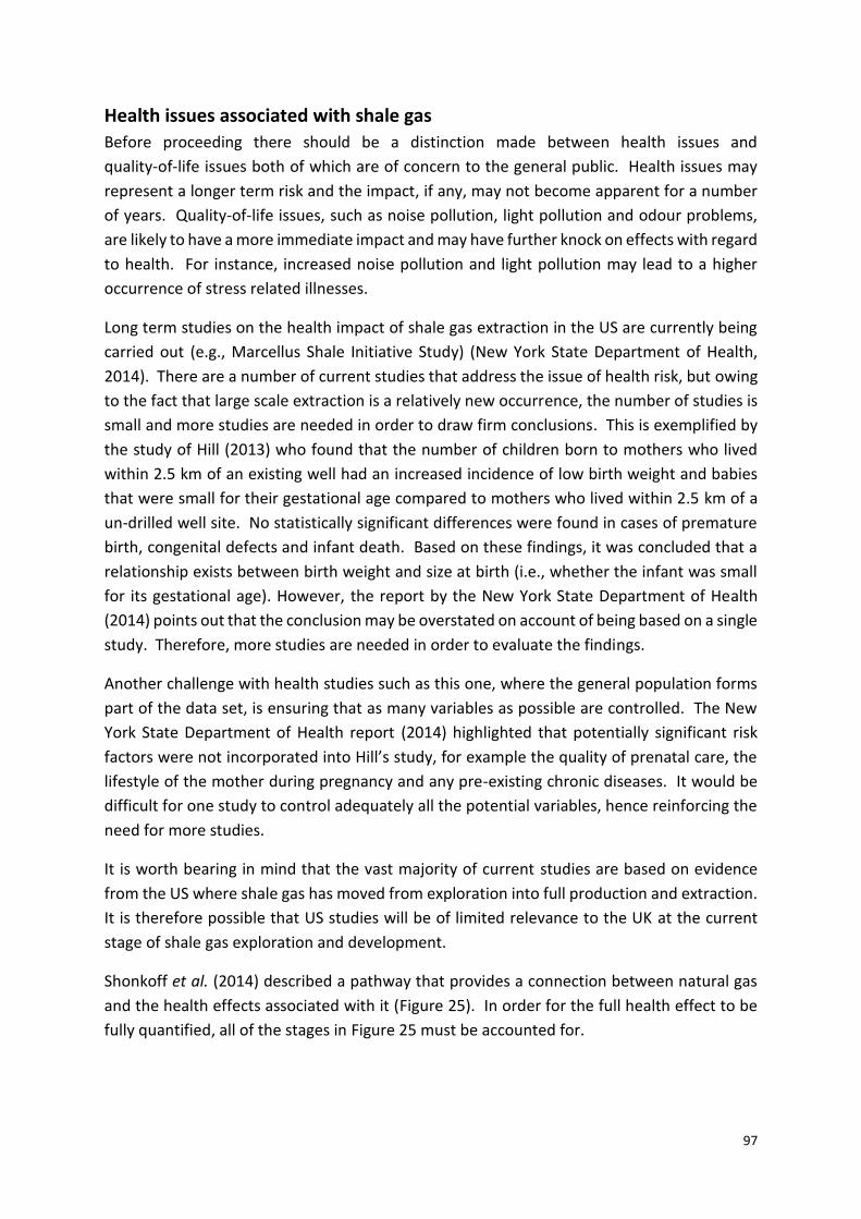
97
Health issues associated with shale gas
Before proceeding there should be a distinction made between health issues and
quality-of-life issues both of which are of concern to the general public. Health issues may
represent a longer term risk and the impact, if any, may not become apparent for a number
of years. Quality-of-life issues, such as noise pollution, light pollution and odour problems,
are likely to have a more immediate impact and may have further knock on effects with regard
to health. For instance, increased noise pollution and light pollution may lead to a higher
occurrence of stress related illnesses.
Long term studies on the health impact of shale gas extraction in the US are currently being
carried out (e.g., Marcellus Shale Initiative Study) (New York State Department of Health,
2014). There are a number of current studies that address the issue of health risk, but owing
to the fact that large scale extraction is a relatively new occurrence, the number of studies is
small and more studies are needed in order to draw firm conclusions. This is exemplified by
the study of Hill (2013) who found that the number of children born to mothers who lived
within 2.5 km of an existing well had an increased incidence of low birth weight and babies
that were small for their gestational age compared to mothers who lived within 2.5 km of a
un-drilled well site. No statistically significant differences were found in cases of premature
birth, congenital defects and infant death. Based on these findings, it was concluded that a
relationship exists between birth weight and size at birth (i.e., whether the infant was small
for its gestational age). However, the report by the New York State Department of Health
(2014) points out that the conclusion may be overstated on account of being based on a single
study. Therefore, more studies are needed in order to evaluate the findings.
Another challenge with health studies such as this one, where the general population forms
part of the data set, is ensuring that as many variables as possible are controlled. The New
York State Department of Health report (2014) highlighted that potentially significant risk
factors were not incorporated into Hill’s study, for example the quality of prenatal care, the
lifestyle of the mother during pregnancy and any pre-existing chronic diseases. It would be
difficult for one study to control adequately all the potential variables, hence reinforcing the
need for more studies.
It is worth bearing in mind that the vast majority of current studies are based on evidence
from the US where shale gas has moved from exploration into full production and extraction.
It is therefore possible that US studies will be of limited relevance to the UK at the current
stage of shale gas exploration and development.
Shonkoff et al. (2014) described a pathway that provides a connection between natural gas
and the health effects associated with it (Figure 25). In order for the full health effect to be
fully quantified, all of the stages in Figure 25 must be accounted for.
98
Figure 25. Visualisation of the environmental exposure pathway for contaminants and pollutants to result in adverse health effects in humans. The source of the contaminants is the well pad and any associated infrastructure; these produce emissions that can potentially contaminate the air, water and soil. The concentrations of these contaminants directly influences the exposure to humans whether it be through air inhalation, contact with skin and eyes, or food and water consumption. Once the level of exposure is established, the dose can be estimated over a given length of time. This, in turn, determines the health effects. (From Shonkoff et al., 2014).
Health complaints reported by the general population living near shale gas wells are skin
rashes, skin, eye and throat irritation, nausea, vomiting, respiratory problems, nosebleeds,
stress, headaches, dizziness, muscle and joint problems and a metallic / bad taste in one’s
mouth (Bamberger and Oswald, 2012; Steinzor et al., 2012; Finkel and Hays, 2013; Rabinowitz
et al., 2015). It should be noted that Steinzor et al.(2012) used a small sample size; 108 people
from 55 households in 14 Pennsylvanian counties. Five of these counties make up 85% of the
surveys submitted meaning that the data is potentially skewed towards particular
characteristics of these counties. The report also neglected to carry out control group surveys
in areas not impacted by gas extraction. The study was not comprehensive insofar as survey
forms were sent out to households and there was no requirement to fill and return them.
One also has to consider that individuals who have had a bad experience related to shale gas
extraction may be more likely to return the surveys than those who have not been affected.
These factors could act to overstate the health impact of these studies and should be treated
with caution. These problems exemplify the limitations of many of the currently published
health studies. The New York State Department of Health report (2014) emphasizes the point
that, although the health complaints may give some indication as to the risks posed to those
living close to a well site, the currently published studies can only reliably be used to generate
hypotheses upon which more thorough future research can be based. Research should centre
around epidemiology studies involving control groups from areas free from extraction of gas
to form baselines and rigorous control of bias associated with sample location, chance
findings and temporality (New York State Department of Health, 2014).

99
Recent studies
The following sections contain detailed breakdowns of three recent major studies on the
potential health impacts of shale gas operations. Each of the reports is examined in detail.
The arguments, together with the evidence cited by the authors, are presented. The
references cited here are, for the most part, those cited in the original reports. A great deal
of evidence for the potential health effects of shale gas operations cited by the reports has
already been discussed and critically appraised in previous sections of this briefing document.
The environmental health impacts review carried out by Werner et al. (2015)
Werner et al. (2015) carried out a review of the currently published evidence for
environmental health impacts of unconventional natural gas exploration and extraction. This
study presents a very thorough review of the currently published literature, hence the
majority of information presented in the following section is drawn from this paper. Any
references that are in the following section are those cited by Werner et al. (2015).
They examined literature published between January 1995 and March 2014. Through
searching online databases of academic literature, the authors initially found 109 relevant
studies. Of these, 7 were considered to be “directly relevant” based on the strength of the
presented evidence (Texas Department of State Health Services, 2010a; Steinzor et al., 2012;
Fryzek et al., 2013; Hill, 2013; Perry, 2013; Steinzor et al., 2013; McKenzie et al., 2014). 38
were considered to be “relevant” and 64 studies were considered to be “not very relevant”.
It was highlighted that all of these studies failed adequately to address long term health
impacts, such as cancer associated with pollution from shale gas sites. The authors argue that
this is reasonable given that shale gas extraction has only taken off in the last few years;
therefore, the effects may not yet be apparent. Studies that make direct associations
between shale gas operations and health impacts were considered to lack the rigour in terms
of methods thus limiting the reliability and applicability of the results. The authors do,
however, highlight the fact that just because there is currently no concrete evidence linking
the shale gas with health problems does not mean that links do not exist and vice versa.
Therefore, more studies are needed in order to understand better what, if any, links exist.
Impact on water
Werner et al. (2015) cite particular chemical additives used in the hydraulic fracturing fluid
that may be cause for concern. Although the amount by volume of chemicals used is low
(approximately 2% or less), because the amount of fluid needed hydraulically to fracture a
well is large (5 million US gallons for several frack stages) this could result in tonnes of
chemical additives being used over the course of the fracturing stages (Finkel and Hays, 2013;
100
Finkel et al., 2013a; Goldstein and Malone, 2013). With regard to ground and surface water
contamination, studies (e.g., Gordalla et al., 2013) have suggested that flowback fluid poses
a more significant hazard than the raw hydraulic fracturing fluid, on account of the salts,
heavy metals and NORM originating from the target formation, that may be present in the
flowback. Flowback can also include polycyclic aromatic hydrocarbons (PAHs), other
hydrocarbons, NORM and salts, all of which present problems for disposal. If chemicals within
the hydraulic fracturing fluid were to enter into the surface and drinking water system they
might result in adverse health effects. This is particularly the case with endocrine-disrupting
chemicals (EDCs), of which there are more than 100 used in the extraction process (Kassotis
et al., 2014). Concentrations of as low as a few parts per billion can be expected to have
adverse effects (Colborn et al., 2011). EDCs chemicals are those that can interfere with the
body’s endocrine (hormone) system (National Institute of Environmental Health Sciences,
2015). They can produce adverse developmental, reproductive, neurological and immune
effects (National Institute of Environmental Health Sciences, 2015). It should be noted that
endocrine disruptors are found in many everyday products such as polycarbonate plastics,
food and cosmetics (National Institute of Environmental Health Sciences, 2015), and exposure
occurs through ingestion of food, dust and water; inhalation of gases and air-borne
particulate matter; and through the skin (World Health Organisation, 2015a).
Few studies have thus far attempted directly to link the chemicals used in fracturing fluids to
the health effects of exposure to specific chemicals. Colborn et al. (2011) discussed how
specific chemicals, if inhaled, ingested or absorbed through the skin, could produce adverse
health effects. Compounds such as (2-BE) ethylene glycol monobutyl ether, acetic acid,
ethylene glycol, isopropanol (propan-2-ol), methanol and sodium nitrate can cause adverse
effects to the skin, eyes, immune system, nervous system and internal organs (Kargbo et al.,
2010; Colborn et al., 2011). Werner et al. (2015) note that these studies did not address the
environmental exposure pathways, actual exposure doses and the causality in terms of health
effects that these chemicals can have on the population living near to shale gas sites. These
essential facts remain to be determined and requires further study.
Impact on health related air quality
Werner et al. (2015) found that the majority of literature published on the impact of shale gas
operations on air quality focused on emission inventories and air sampling, not on direct
health impacts, although some characterisation of the risk associated with the emissions was
carried out. It should be noted that the authors also found that there is a geographical bias
in the current literature. The vast majority of current literature comes from Garfield County,
Colorado, although there is some research from Texas and Pennsylvania. Of the published
studies, two general areas of concern were found. First, hazard descriptions of air-borne
pollutants and how these are released into the atmosphere, and secondly, the health
concerns associated with the pollutants.
101
The most commonly cited pollutant is methane from fugitive emission sources. Other
pollutants that can be released during shale gas operations have been cited as potentially
harmful; these include benzene, carbon monoxide, hydrogen sulphide, nitrogen oxides,
sulphur dioxide and VOCs (Witter et al., 2008b; Colorado Department of Public Health and
Environment, 2009; Colborn et al., 2011; Kaktins, 2011; Zielinska et al., 2011; Down et al.,
2012; Weinhold, 2012; Kibble et al., 2013).
Werner et al. (2015) found that data on inhalation-related toxicity is limited, with only a few
studies providing data that are of sufficient utility. They provide one example where a study
identified 86 contaminates, the data for 65 of which were not extensive (Colorado
Department of Public Health and Environment, 2010). Therefore, the potential health impact
could be underestimated. The authors suggest that concurrent bio-monitoring studies should
be carried out with air monitoring studies because, whilst the amount of emissions can be
monitored, the amount that is actually inhaled by members of the population is not
measured. Few examples of bio-monitoring studies were found, but one such study was
carried out by the Texas Department of State Health Services (Texas Department of State
Health Services, 2010a). They collected blood and urine samples from 28 people living in and
around the town of Dish with the aim of investigating the impact of VOCs on local
communities (Texas Department of State Health Services, 2010a). They found that VOC levels
were not consistent with those that would be expected for community wide exposure to shale
gas related VOCs and pollutants. However, the study also considered that their results could
be affected by exposure to other factors, smoking, disinfectant by-products in drinking water
and workplace exposure which were not accounted for. Only one sampling period was carried
out during the study. Therefore, changes in VOC exposure with time could not be measured
(Texas Department of State Health Services, 2010a). These factors represent a shortcoming
of the sampling protocols used in this study, and others carried out to date, and indicate the
need for appropriate sampling to be carried out in future studies. If this is done, it may be
possible to differentiate between VOC exposure originating from shale gas operations and
those from other sources in addition to determining the variation in VOC levels with time.
Pollutants in soil
Few studies addressing the issues of soil contamination as a result of unconventional natural
gas operations were found (Coons and Walker, 2008; Witter et al., 2008b).
Contamination of soils mainly occurs through spills and leaks on-site but can also occur when
the drilling cuttings are being stored, transported and disposed of (Zoback et al., 2010). Some
of the same pollutants cited as potentially dangerous when emitted from fluids, e.g. benzene,
can also contaminate land by either adsorbing into or absorbing onto soil particles. This
creates a residue that can leach upon interaction with rain or snowmelt. Pollutants can also
be inhaled, absorbed or otherwise ingested (Coons and Walker, 2008; Witter et al., 2010).
102
Werner et al. (2015) make the point that data on soil quality and contamination, or lack
thereof, in relation to shale gas operations is lacking. They also highlight the need for baseline
studies in order fully to quantify the impact of any contamination.
Occupational health
The above discussion has only addressed the issue of the hazard and risks posed to the wider
population by shale gas operations. However, the hazard and risk to the on-site employees
is of significance as they will come into contact with substances, such as flowback fluid stored
in tanks, on a daily basis. Studies have highlighted that safety hazards in the oil and gas
industry are well documented but health hazards and chemical exposure risks are less well
studied (Coussens and Martinez, 2013; Esswein et al., 2013). A major occupational health
hazard that could potentially affect on-site employees is that of crystalline silica (i.e., sand
and dust) as, when inhaled, can result in silicosis, lung cancer, tuberculosis, autoimmune
diseases and kidney disease (Laney and Weissman, 2012; Esswein et al., 2013). Silicosis is of
particular concern as it has a long latency period (as long as decades) between exposure and
the development of symptoms (Laney and Weissman, 2012). A recent exposure assessment
study of crystalline silica on shale gas sites in the US found that many of the samples taken
were above the acceptable exposure limit (Esswein et al., 2013). As would be expected,
workers using certain equipment, i.e., sand mixers, were exposed to the greatest amount of
crystalline silica (Esswein et al., 2013). Building site and quarry workers can be exposed to
very high levels of silica dust exposure.
Two studies were found that examine the potential effect of drilling fluid (mud) on the health
of on-site employees (Broni-Bediako and Amorin, 2010; Searl and Galea, 2011).
Broni-Bediako and Amorin (2010) found that exposure to fluid was mainly through inhalation
of vapour mist, dermal or oral contact with vapours, aerosols and dust. Searl and Galea (2011)
similarly found that the main health risks are inhalation of vapour and aerosols. They also
said that long term exposure can increase the risk of chronic respiratory illnesses in addition
to neurological problems potentially including dementia. It should be noted that the risks
associated with exposure to fluids associated with shale gas operations will vary from site to
site as it is highly dependent upon the composition of the fluids used.
Noise pollution was also cited as a potential health hazard by (Witter et al., 2014). Prolonged
exposure to noise emanating from compressors, generators, drilling, diesel engines,
mechanical brakes, radiator fans and heavy machinery can result in noise-related health
problems, such as deafness and tinnitus (Witter et al., 2014). This applies to many types of
industrial activity.
103
Health impacts from infrastructure associated with shale gas operation
When compared to other health issues, i.e., air and water pollution, the number of studies
published regarding the health impact of shale gas related infrastructure is much lower.
A study by La Plata County (2002) considers that, although the drilling sites may be situated a
sufficient distance apart as to minimise the amount of noise pollution coming from a single
site, the cumulative effect of multiple sites may be larger depending on each site’s stage of
operation. Low frequency (infrasonic) noise pollution, i.e., that emanating from the
continuous running of generators, has the potential to cause various health problems, i.e.,
stress, annoyance, irritation, fatigue, headaches, unease, disturbed sleep and cardio vascular
problems (Witter et al., 2008a; Witter et al., 2010; Witter et al., 2013).
Werner et al. (2015) found that no studies had investigated the impact of light pollution
resulting from shale gas operations, whether on humans or wildlife. Some studies have
suggested measures, such as directional lighting, modified drilling rig placements and glare
restrictions, that can reduce the potential for light pollution (Witter et al., 2010; New York
State Department of Environmental Conservation, 2011), however, no studies have gone as
far as to assess the risk of the light pollution hazard. This may be significant as sites will likely
be running 24 hours a day. Recent studies from other industries has suggested a link between
artificial light exposure and increased cancer risk (Witter et al., 2008a). This of particular
concern to those employees working night shifts, as they will have prolonged exposure to
artificial light. Again, this hazard applies in many spheres of employment.
Increases in traffic flow may occur around areas of shale gas operations but this has not been
subject to any in-depth studies from a health perspective, as opposed to road safety. Any
increase in traffic flow will likely be site specific and be influenced by the existing
infrastructure, i.e., the number of wells being drilled and the number of other sites located
nearby. In addition, the traffic flow will vary depending upon the drilling stage. Gas and
particulate emissions from heavy goods vehicles transporting material to and from sites has
been considered to result in increased air pollution around shale gas sites (Hill, 2013). UK
planning authorities refusing permits have several times appealed to the unacceptability of
increased traffic as grounds for refusal, so it is important that this perceived hazard is studied
properly and objectively.
Social impacts
Werner et al. (2015) identified three health related social impacts related to unconventional
natural gas operations; symptomatological, risk perception, and governance and regulation.
In terms of symptomatological studies, surveys of residents living in near to shale gas
operations in the US tend to feel that their health is being adversely affected (Steinzor et al.,
2012; Steinzor et al., 2013). The members of the local population that responded to these
104
surveys conveyed concerns about what they perceived to be health symptoms directly related
to natural gas operations. These symptoms were nose, eye, and throat irritation, respiratory
symptoms, nausea, nosebleeds, sleep disturbance, rash, headaches, ringing in ears,
abdominal pain or cramping, extreme drowsiness, fatigue, and weakness (Subra, 2009, 2010;
Texas Department of State Health Services, 2010a; Bamberger and Oswald, 2012; Steinzor et
al., 2012; Saberi, 2013; Steinzor et al., 2013). However, Werner et al. (2015) found no
evidence of direct cause and effect. Adgate et al. (2014) consider that many of these non-
specific symptoms could be attributed to psychological stress associated with having a nearby
unconventional natural gas site. They also consider that this could, itself, be seen as a health
risk but has not yet been studied as one.
As would be expected, the number of reported symptoms associated with shale gas
operations decreases with increasing distance from the operation site (Steinzor et al., 2012).
This could either be an indication that there is a direct link between shale gas operations and
health effects or it could indicate the psychological impact of living near to a site.
One of the most commonly reported concerns is that of odour, with local residents reporting
a range of odours, i.e., unidentified gas, sulphur, burnt butter, propane, sickly-sweet smells
and ‘chemical-like’ smells (Subra, 2009, 2010; Steinzor et al., 2013).
Cancer incidence, as a result of benzene emissions from shale gas sites, was also cited as a
social concern by communities in Texas. In a series of studies, the Texas Department of State
Health Services (Texas Department of State Health Services, 2010a, b, 2011), the cancer
incidence was investigated. The results from the most recent study found no correlation
between shale gas operations and the incidence of various types of cancer. Specifically
childhood leukaemia, childhood brain / central nervous system cancers, all-age leukaemia,
and all-all non-Hodgkin’s lymphoma, in the surrounding communities were in the expected
ranges for both sexes (Texas Department of State Health Services, 2011). However, the
incidence of breast cancer was statistically significantly higher than expected. This was
attributed to the rapid increase in population around areas of shale gas operations (Texas
Department of State Health Services, 2011). The study also considered that the number of
cancer cases upon which the study was based was likely to have been underestimated
because the population data was obtained from the 2000 Census (Texas Department of State
Health Services, 2011).
Another study, by Fryzek et al. (2013), investigated the incidence of childhood cancers at
different stages in the drilling process. They found that the occurrence of all but one cancer
type was near to expected levels both before and after drilling. There was found to be a slight
increase in the standardised incidence ratio for central nervous system tumours after drilling
had taken place. Overall, the authors concluded that there was no increase in the incidence
of cancer in communities living near to drilling sites. Goldstein and Malone (2013) disputed
this conclusion as being ‘unfounded’. Werner et al. (2015) pointed out that the timeframe
for the studies (1995-2009) does not encompass the complete development of shale gas in

105
the Marcellus region therefore the results and conclusions drawn by Fryzek et al. (2013) are
of limited applicability.
Many generalised symptoms are difficult to attribute directly to shale gas developments,
however, members of the local population have reported their symptoms becoming less
prominent when they leave the area around shale gas sites (Steinzor et al., 2013). Current
epidemiological studies (Texas Department of State Health Services, 2010b, 2011; Fryzek et
al., 2013) have not linked cancer incidence to shale gas operations. There is, however, still a
need to expand the number of studies and to conduct more research into long term
epidemiology.
Werner et al. (2015) found that the public’s perception of hazard must be considered as a
factor. Perry (2012) found that the public create their own perception of hazard and risk
based on the available scientific information and regulatory information. In turn, the
uncertainty associated with perceived risk can cause health related complaints, i.e., stress and
anxiety (Perry, 2013). Werner et al. (2015) concluded that there is a real need for studies
comparing the public perception of risk to actual risk data.
Public Health England 2013 Report
Public Health England (PHE), an executive agency of the Department of Health, carried out a
review of the potential public health impacts of exposures to chemicals and radioactive
pollutants resulting from shale gas operations (Kibble et al., 2013). The review was carried
out, specifically, by the PHE Centre for Radiation, Chemical and Environmental Hazards (CRCE)
who examined literature and data from countries where commercial-scale shale gas
extraction operations were already underway.
The review highlighted that potential risks to human health cited in literature, e.g., fugitive
emissions and surface spills of hydraulic fracturing fluid, were a result of either poor
regulation or an operational failure. The difference in potential human impact between single
well exploratory sites and full-scale extraction involving multiple wells, the cumulative impact
of which may be more considerable, was also emphasised. The overarching conclusion drawn
from the study is that the potential risks to public health from emissions will be minimal if the
operations are run and regulated properly.
Aside from the main conclusion, the review made eight recommendations:-
1. PHE should continue to work with regulators to ensure that all aspects of shale gas
exploration and extraction in order to ensure that all risks are appropriately assessed.
2. Baseline environmental monitoring is required in order to assess the impact of shale
gas operations on environmental, and hence public, health. The development of
emission inventories should be considered as part of the regulatory regime.

106
3. Effective monitoring is required throughout the entire lifetime of the site including the
post-production abandonment phase.
4. The broader socioeconomic impacts, such as increased traffic and the impact on local
infrastructure should be considered during the planning stage of any operation.
5. The chemicals that are used in the hydraulic fracturing fluid should be publicly
disclosed and assessed prior to use. The review notes that any potential risk to the
public posed by the chemicals will be dependent upon the exposure pathway,
together with the total volume, concentration and fate of the chemicals. It is
considered by the authors that these risks will be assessed during the regulatory
environmental permitting process.
6. The type and composition of gas will vary on a site by site basis, and as such, the risk
assessment should be carried out on a site-by-site basis.
7. Evidence from the US indicates that well integrity, appropriate storage and
management of hydraulic fracturing fluid and waste products are key to ensuring that
risks are minimised, therefore, the appropriate regulatory control will need to be put
in place. Again, implementation details will likely vary from site to site.
8. Characterisation of potentially mobilised natural contaminants, i.e., NORM and
dissolved minerals originating from the target formation, is needed.
Air quality
The PHE review said that, at the time of publication, there was no published data regarding
emissions from UK shale gas sites, nor has there been any emission data published from the
hydraulically fractured, conventional tight gas sand well at Elswick, Lancashire, where
production has been carried out since 1993. At this particular site, gas was extracted from
low permeability sandstone via hydraulic fracturing of a vertical well. Note that the degree
of fracturing required was far less than that required to stimulate gas production from shale.
The PHE review considered that emissions from single sites will likely be small, intermittent
and not unique to shale gas operations, i.e., comparable to certain other industries. However,
the main environmental hazard comes when the density of drilling pads and wells per pad
increases, producing potentially a larger cumulative impact (Kibble et al., 2013). Common
compounds that might be emitted from shale gas sites (i.e., nitrogen oxides (NOx) VOCs and
particulate matter) can produce secondary pollutants, e.g., ozone (O3). However, these
pollutants can also be produced from other industry sources and transport (Kibble et al.,
2013). This reinforces the need to establish background emission levels prior to any drilling
taking place.
In terms of published evidence, the review cites a study by Zielinska et al. (2011) in which air
pollutants from Barnett Shale sites were characterised. The authors found that, in addition
to methane, 70 different VOCs were found, the most abundant of which were ethane,
propane, n-butane and pentane. These VOCs made up approximately 90% of the total

107
emissions. The remaining 10% was made up by 2- and 3-methylpentane, n-hexane, methyl-
cyclopentane, cyclohexane, 2-methylhexane, 1-heptene, methylcyclohexane, n-heptane, and
n-octane (Zielinska et al., 2011). PAH (benzene, toluene and xylenes) account for 0.1-0.2% of
non-methane VOCs (Zielinska et al., 2011). The main source of the emissions was found to
be from malfunctioning condensation tanks.
Between 2008 and 2010, Rich et al. (2014) carried out emissions work in the Dallas and Fort
Worth areas overlying the Barnett Shale. The aim of the study was to attempt to establish a
“fingerprint” of chemicals that could be associated with shale gas operations in residential
areas. To do this, the authors collected ambient air samples from residential areas within
61 m of shale gas extraction / production. A total of 50 sampling data sets were obtained and
analysed. Most areas had methane levels (a mean of 11.99 ppmv (parts per million by volume)
and a median of 2.7 ppmv) higher than background urban concentrations (1.8-2.0 ppmv).
Other chemical components were found to correlate with the presence of methane, for
instance 3-methylhexane. The researchers found that seven chemicals (o-xylene,
ethylbenzene, 1,2,4-trimethylbenzene, m- and p-xylene, 1,3,5-trimethylbenzene, toluene and
benzene) could potentially provide a pollution signature for shale gas operations. However,
there are limitations to the study which are pointed out by the authors. These include the
small sample size and that correlation with a common source does not mean other sources
are not contributing to the correlation, i.e., other sources of chemicals and methane could
not be distinguished from those from shale gas operations. Rich et al. (2014) suggest that a
further study with a larger sample size and more rigorous analysis be carried out.
Roy et al. (2014) developed an emissions inventory for the development, production and
processing stages of shale gas operations in the Marcellus Shale for 2009 and projected 2020.
Based on the 2009 estimates, operations in the Marcellus Shale may account for 6-18% (12%
average which equates to 129 tons per day) of the NOx emissions and between 7 and 28%
(12% average which equates to 100 tons per day) of the anthropogenic VOC emissions, with
an average contribution of 12% (100 tons per day) in the Marcellus region. The study also
examined particulate matter. The authors consider that shale gas operations will not make a
significant contribution to particulate matter emissions in the Marcellus area. It should be
noted that the 2020 estimates are subject to considerable uncertainties due to the fact that
assumptions were made regarding future control measures on emissions (Kibble et al., 2013),
i.e., if more stringent regulations are introduced, emissions will fall. Certain unknown
parameters also introduce uncertainties related to the emission estimates. For instance, the
engine on-time of the drilling rigs is considered to cause uncertainties in NOx estimates (Roy
et al., 2014).
Using daily air samples collected at the National Oceanic and Atmospheric Administration
Boulder Atmospheric Observatory, Weld County, Colorado, together with a road based air
sampling survey, Pétron et al. (2012) examined the emissions from shale gas operations in
the Denver-Julesberg Fossil Fuel Basin, Colorado. Air samples were analysed for methane and

108
non-methane VOCs (specifically propane, n-butane, i-pentane, n-pentane and benzene). A
range of emissions producing activities took place in the basin, including oil and gas
operations (both conventional and un-conventional), a landfill site, feedlots, a water
treatment plant and automobiles. After being corrected for wind direction, the results
suggested that strong alkane and benzene signatures were coming from the north-eastern
Colorado. The main activity that produced such compounds was oil and gas operations. The
authors considered that flashing of gas from condensate tanks and venting and leaking of
wells as being key emission sources.
The type of emissions produced by each site will vary depending upon whether the gas is wet
or dry. Wet gas is produced when pressure/temperature conditions of burial were not so high
as to preclude the formation of liquid hydrocarbons. Thus wet gas contains other
hydrocarbons, e.g., butane and ethane, while dry gas does not. These other hydrocarbons
are known as natural gas liquids (Kibble et al., 2013). As wet gas contains other hydrocarbons,
there is the potential for these sites to produce more VOC emissions. Evidence from the US
(Roy et al., 2014) has shown that the gas composition can vary within a single shale formation.
The Marcellus shale is known to be mainly dry gas but in southwest Pennsylvania, wet gas is
found. This highlights the need to asses each operation site on a case-by-case basis.
In summarizing the impact of shale gas operations on air quality, the review highlights the
fact that any emissions are highly dependent upon the phase of well development,
operational practices, geology, local topography, meteorology, the type of activities and on-
site equipment. Therefore, the type and volume of emissions will be unique to each site
whilst also varying with time. The review considers that, because of these variations, it is
impossible to directly apply the findings from the US to UK shale gas operations (Kibble et al.,
2013). However, the information from the US does provide some indication of the emission
sources and how to go about managing them.
In terms of further work, PHE suggest that, because the type of gas produced will vary from
site to site, detailed risk assessments will need to be carried out at each shale gas site. Air
quality monitoring should be carried out both before and during any operation. Of particular
importance will be the need to carry out regional scale monitoring due to the potentially
significant cumulative effect of numerous well pads and wells.
Radon
Radon-222 is a product of the uranium-238 decay chain with radium-226 being the immediate
precursor. It has a radioactive half-life of 3.8 days and is released from most rocks and soils,
although the amount that is released is dependent upon mineralogy. Radon emits alpha
particles which are harmless unless ingested by breathing or via groundwater. Radon
migrates through both fractures in rocks and pore spaces in soils; the rate of migration is
controlled by the transmission characteristics of rocks, soils and underground fluids.

109
Exposure to natural radon sources accounts for 84% of the annual radiation exposure
experienced by the members of the general population (Watson et al., 2005). Shale gas wells
have the potential to act as conduits for radon migration to the ground surface if the well
passes through radon-containing formations (Kibble et al., 2013).
Radon concentrations in the open air are generally low (5-15 Bq/m3 (World Health
Organisation, 2015b)); however, where radon can be drawn into buildings, on account of
pressure gradients, the concentration is can be much higher (thousands of Bq/m3) (Kibble et
al., 2013). Therefore, indoor radon exposure poses the greatest hazard to the general
population. In the UK, the typical annual exposure to radon associated with natural gas is
4 µSv/yr (based on typical natural gas usage and a concentration of 200 Bq/m3) (Dixon, 2001).
This is smaller than the levels of radiation from other every day sources, for instance, the
typical yearly exposure is less than that of a chest X-ray (100 µSv) and smaller than the hourly
dose rate of travelling in a plane at a cruising altitude of 12 km (5 µSv/hour) (STUK - Radiation
and Nuclear Safety Authority, 2012). Note that the average UK radon exposure is
1,300 µSv/yr.
The literature review carried out by Kibble et al. (2013) found no UK specific information on
radon associated with shale gas operations. There is, however, information from the US
relating to radon in natural gas. Kibble et al. (2013) cite studies by Johnson (1973) and
Resnikoff (2012) who proposed values of radon associated with natural gas operations of
1,370 Bq/m3 and 1,365-95,300 Bq/m3 respectively. The latter figures proposed by Resnikoff
(2012) are obtained for estimated radon concentrations at the wellhead. The same study also
says that, depending on gas treatment, processing and transport length, the radon
concentration in the gas delivered to customers can be as high as 72,000 Bq/m3, resulting in
indoor radon concentrations of 20 Bq/m3. Kibble et al. (2013) point out that Resnikoff (2012)
did not account for mixing of natural gas from shale operations with gas from other sources
which could influence the radon content.
A study by Rowan and Kraemer (2012) found radon concentrations of 37-2,923 Bq/m3
between the wellhead and water-gas separator at 11 drilling sites in the Marcellus Shale. By
applying the values of Dixon (2001) and the upper concentration values of radon found at the
wellhead by Rowan and Kraemer (2012), Kibble et al. (2013) determined that exposure to
members of the public in the UK would be 60 µSv/yr. This is approximately 0.5% of the annual
radon exposure of 1,300 µSv/yr. Short-term outdoor radon concentrations of up to
165 Bq/m3 were measured around a shale gas site in Colorado by Burkhart et al. (2013). The
authors note that this is higher than normal outdoor levels (5-15 Bq/m3 (World Health
Organisation, 2015b)); however, they were unable to differentiate between sources.
In terms of radon in water, ingestion and degassing resulting in airborne radon are cited as
the most significant sources of radon exposure (Kibble et al., 2013). Kibble et al. (2013) say
that the largest radon concentrations are found when groundwater comes into contact with
crystalline rocks (igneous / metamorphic rocks). A study by Otton (1992) is cited as evidence
110
of increased radon concentration around hydraulic fracturing wells; although Kibble et al.
(2013) note that the cause of the increased radon concentration was not established, it could,
therefore be a natural occurrence. Assuming migration of radon from shale formations into
groundwater as a result of hydraulic fracturing, Myers (2012) determined that the time
required for migration via advection would result in any radon decaying to the point where it
would no longer pose a threat to humans. Overall, Kibble et al. (2013) consider that, due to
the short half-life of radon and the depth at which hydraulic fracturing will take place in the
UK, any radon that enters into the groundwater system would have minimal impact.
Radon, because of its solubility, can be present in flowback fluid. Kibble et al. (2013) found
no information directly relating to the concentration of radon in flowback fluid.
Measurements of alpha particles, which are emitted, together with beta particles, as radon
decays, in the Preese Hall flowback water have been made by the EA (Environment Agency,
2011). Gross alpha particles were found in concentrations of 10-200 Bq/L; radium-226, the
pre-cursor to radon, was found in the fluid. This is considered to indicate the probable
presence of radon (Kibble et al., 2013). Note that, as pointed out previously, alpha particles
need to be ingested in order to pose a hazard. Degassing of radon at the wellhead is
considered by Kibble et al. (2013) to have the potential to result in localized increases in
radon. As such, the authors consider it to be an occupational hazard, for instance, to workers
in the unlikely event of eating their sandwiches at the wellhead, as opposed to a public health
hazard.
Kibble et al. (2013) conclude that radon could present a highly localized hazard on-site but is
not likely to lead to a significant public health hazard.
NORM
NORM are considered by Kibble et al. (2013) to be present in cutting fluids, drilling muds and
flowback fluids. NORM concentrations have been measured by the EA in the flowback fluids
from the Preese Hall site and found levels to be similar to that found in granite (Environment
Agency, 2011). The fluid contained high levels of sodium, chloride, bromide and iron
(Environment Agency, 2011). Levels of lead, magnesium and zinc were higher than those in
the mains water used in the initial fracturing fluid (Environment Agency, 2011). Naturally
occurring radionuclides of potassium-40, lead-212, lead-214, bismuth-214, radium-226 and
actinium-228 were found. The highest concentrations in fluid were associated with radium-
226 (14-90 Bq/L) while the radium-226 activity of suspended solids was found to be 2.5-
7.2 Bq/kg. Kibble et al. (2013) say that these values are consistent with the range of values
found elsewhere in Europe (0-200 Bq/L and 5-900 Bq/kg).
With regard to assessing the health risks, Kibble et al. (2013) emphasise the challenges posed
by accurately determining the exposure of the general public to NORM. Specifically, they
describe the need to have detailed knowledge of the operation, the everyday habits of both
111
the workers and local population, and information about the treatment and disposal of any
radioactive material. There is also a need for differentiation between the hazards posed by
drilling waste and those posed by flowback fluid.
Kibble et al. (2013) consider that the UK has a history of dealing with NORM contaminated
drilling waste that has been produced from traditional hydrocarbon operations. As such,
there are procedures and waste management plans in place to ensure that waste is properly
handled and disposed of. A potentially more challenging prospect is that of NORM
contaminated flowback fluid. The authors point out that the waste treatment plants will have
specifically to address factors including the storage, treatment, transport and disposal of the
fluid.
(Kibble et al., 2013) are also of the opinion that, based on current measurements from the
Preese Hall site together with measurements and assessments of the radioactivity exposure
experienced by offshore oil and gas workers, it is not expected that shale gas operations
would pose a radiological hazard to the public. They also consider that the current regulatory
system is capable of protecting both the general public and workers from the radioactivity
hazards arising from NORM. Despite this, the authors highlight the need for data on UK
NORM levels as this is the only way accurately to predict potential exposure in the UK.
Water and wastewater
The PHE report highlights the importance of ensuring that the water needed for the hydraulic
fracturing process is extracted from a sustainable source (Kibble et al., 2013). Potential
problems associated with the storage of the hydraulic fracturing fluid are also raised. The
authors say that, if fracturing fluid is stored on site, there is an increased chance of
contamination of surface waters if a spill takes place due to poor handling or
mismanagement. In addition, it is suggested that, because of the volume fluid returning to
the surface as flowback, sites may not have the processing capacity to deal with all the waste.
Although the authors acknowledge the potential for recycling of fracturing fluid, they also say
that the volume that can be recycled is dependent upon the salinity and concentration of
chemical constituents accumulated during the fracturing and flowback process.
Kibble et al. (2013) say that there is currently no peer reviewed literature on the impacts of
shale gas operations on water in the UK or elsewhere in Europe. However, there have been
some non-peer reviewed studies that have looked at the potential impact on drinking water
sources (Broderick et al., 2011; House of Commons, 2011; The Royal Society and the Royal
Academy of Engineering, 2012). As has been discussed in the water contamination section,
of this briefing document, contamination of ground and surface water has taken place in the
US as a result of shale gas operations. The Royal Society and the Royal Academy of
Engineering report (2012) also highlighted the need for baseline methane measurements in
groundwater prior to any operations being undertaken. The BGS are currently in the process
112
of establishing these baselines. The analysis of the Preese Hall flowback fluid showed high
levels of sodium, chloride, bromide and iron together with levels of lead, magnesium, zinc,
chromium and arsenic elevated above the concentration found in the water used to form the
basis of the fracturing fluid (Kibble et al., 2013).
Kibble et al. (2013) cite studies discussed previously as evidence of water contamination
resulting from shale gas operations (Osborn et al., 2011; Warner et al., 2012; Jackson et al.,
2013; Molofsky et al., 2013; Vidic et al., 2013; Warner et al., 2013). The authors also discuss
a study by the Massachusetts Institute of Technology (2011) which reviewed 43 incidences of
water pollution that took place between 2005-2009. The study found that loss of well
integrity is the major cause of contamination (20 of the 43 incidents) with surface spills being
the second most important cause (14 of 43 incidents). Contamination took place via
inadequate cementing, inadequate casing installation, hose leaks at the surface, overflowing
pits and failure of the pit lining. As has been noted previously, the use of open pit storage is
prohibited in the UK; therefore the potential for contamination events from these last two
sources will be non-existent. A study by Goss et al. (2013) which analysed groundwater
benzene, toluene, ethylbenzene and xylene levels after surface spills had taken place in the
US is also cited in the PHE report. The study found that levels of these contaminants exceeded
US the safe drinking water limits in some samples, however, the remedial action taken by the
operators reduced these levels effectively.
The PHE report addresses concerns regarding drinking water contamination during hydraulic
fracturing by saying that 99% of water that enters people homes comes from water
companies that have not only carried out treatment on the water, but also have a number of
additional quality control measures in place (Kibble et al., 2013). These include
measurements of water quality as it leaves the treatment facility in addition to random
samples taken from homes. Kibble et al. (2013) see it as unlikely that contaminated water
would enter into homes on account of this regulatory scheme. The authors also consider
contamination as a direct result of hydraulic fracturing, i.e., upwards migration of fluids, to
be a minimal risk owing to a lack of current evidence that suggests that fractures can migrate
a sufficient distance to interact with groundwater.
Citing a publication by the Chartered Institute of Water and Environmental Management
(2014), Kibble et al. (2013) point out the importance of considering the following when
planning a shale gas operation; baseline monitoring; monitoring throughout the lifecycle of
the well; the potential contamination resulting from a loss of well integrity; the need to follow
best operational practices; the transport, management and storage of chemicals, hydraulic
fracturing fluid and flowback fluids; and the treatment of flowback fluids. The Chartered
Institute of Water and Environmental Management (2014) suggest hydraulic fracturing
should not be allowed to take place in areas where there is a risk to groundwater. In addition,
it is considered that the relationship between groundwater and the target shale formations
113
be examined before any drilling takes place (Chartered Institute of Water and Environmental
Management, 2014).
Kibble et al. (2013) note that Water UK, the representatives of the UK water industry, and
UKOOG have signed a memorandum of understanding that both bodies will work together
to minimise the environmental impact of any future shale gas operations. This approach
includes baseline monitoring, water management and waste water disposal (United Kingdom
Onshore Operators Group, 2013b).
Kibble et al. (2013) highlight the potential environmental impact of waste waters and
flowback fluid once they have been treated at the appropriate waste management facilities.
The authors cite the study carried out by Warner et al. (2013) which has been previously
discussed in the surface water contamination section. In addition, studies by Voltz et al.
(2011), Hladik et al. (2014) and Shariq (2013) are also cited. The study by Voltz et al. (2011)
found that contamination of tributaries of the Ohio River by barium, strontium and bromide
had taken place after treated waste water from shale gas operations had been released. The
authors also suggested that the increased bromide concentration could lead to the formation
of disinfectant by-products (DBP) in chlorinated drinking water. The same suggestion was
made by Hladik et al. (2014) who found, from examination of waste water treatment plants
in Pennsylvania that accepted waste from both conventional and unconventional
hydrocarbon operations, that the level of DBPs was increased compared to treatment plants
not accepting waste from hydrocarbon operations. Shariq (2013) raised the issue of treated
and diluted wastewater being used to irrigate crops. Kibble et al. (2013) say that, although
there is little data on the issue, the practice is unlikely to be permitted in the UK.
Hydraulic fracturing fluid
Kibble et al. (2013) found no peer reviewed literature relating to the composition and use of
hydraulic fracturing fluid in the UK. This is partly down to the lack of drilling activity but also
to the need to consider each site individually. The composition of the hydraulic fracturing
fluid that has been used at the Preese Hall site can be found in Appendix 2.
Kibble et al. (2013) cite studies by Kassotis et al. (2014) and Colborn et al. (2011), the latter of
which have been discussed as part of the Werner et al. (2015) study, as presenting evidence
of the potential effect of the chemicals used in the hydraulic fracturing process. The study by
Kassotis et al. (2014) was motivated by the authors estimate that there are potentially 750
chemicals and components that can be used in the hydraulic fracturing and gas extraction
processes. More than 100 of these chemicals and components are known or are suspected
to be endocrine disruptors.
Kassotis et al. (2014) investigated 12 EDCs used in hydraulic fracturing fluids in the Garfield
County, Colorado. 39 unique surface and ground water samples were taken at 8 sites
including 2 reference sites and the main drainage basin for the sample sites (Colorado River).

114
These sample collection sites were those that had experienced some form of surface spill or
leak. Samples collected from drilling-dense areas showed higher concentrations of these
EDCs compared to reference sites where limited, or no, drilling took place. This suggests that
baseline monitoring is needed before drilling starts in order better to establish pre-existing
levels of EDCs. Samples from the Colorado River displayed moderate amounts of EDCs, larger
than the control sites but lower than the spill / leak sites. The study considered that spills and
leaks result in higher concentrations of EDCs in surface and ground water. It should be noted
that Kassotis et al. (2014) do not categorically state that water contamination took place due
to drilling activity, but rather they suggest that increased EDCs may be a result of drilling
activity. In addition, both naturally occurring chemicals and those originating from drilling
activity were measured in this study, although the contribution from natural sources was
considered to be minimal. The study also gives no indication given regarding the volume of
leaked fluid. Kassotis et al. (2014) concluded that shale gas activity may result in an increase
in endocrine disrupting compounds in groundwater. Kibble et al. (2013) point out that the
study was carried out using an in-vitro (cell culture) test system and that endocrine disrupting
activity found in such test systems may not necessarily translate into endocrine disrupting
activity in in vivo systems (i.e., entire organisms). They can, however, prove to be useful in
informing decisions regarding further toxicity testing in addition to indicating potential modes
of action (i.e., changes at a cellular level) (Kibble et al., 2013).
The PHE report considered that, although the volume of chemicals used in the process of
hydraulic fracturing is small, the potential impact of multiple wells could be considerable. The
prospect of these chemicals being stored on-site could also prove to be hazardous. Because
of this, Kibble et al. (2013) emphasise the need for transparency in disclosing the chemicals
in fracturing fluids and the need for such chemicals to be subjected to independent
assessment before use. This will allow a thorough hazard and risk assessment to be carried
out. This is particularly significant as the composition of fracturing fluid will likely vary from
site to site. Suitable accident management plans and enforcement of best practices and
regulations are also considered by Kibble et al. (2013) to be key to minimising the impact of
any accidents that might occur on-site.
New York State Department of Health 2014 report
A similar public health review was carried out by the New York State Department of Health
(2014). Like the PHE study, the New York State report covered a range of potential areas that
could impact on human health, specifically, air pollution, climate change impacts, drinking
water impacts, soil and water contamination, inadequate treatment of wastewater,
earthquakes and socioeconomic impacts.
The review determined that the impact on public health is difficult to assess fully as the
hazards and associated risks will vary spatially on account of differing well pad densities,
populations and baseline environmental conditions. The authors consider that, because of

115
the dispersed nature of the potential operation locations in New York State, the chance of
equipment failure and / or process failures is increased (New York State Department of
Health, 2014). This, in turn, could lead to an increased cumulative risk of exposure. However,
if appropriate regulations were in place and adhered to, one would assume that the hazards
associated with equipment and process failures should be reduced although a guarantee of
absolute safety cannot be made (New York State Department of Health, 2014).
The New York State Department of Health (2014) review highlighted the lack of long term
studies on the health impacts of shale gas exploration and extraction. At the time of
publication, these long term studies had either not been published or had not been started
(New York State Department of Health, 2014). The available information was considered to
be only exploratory in nature and demonstrates considerable uncertainties in the human
health impact of shale gas operations (New York State Department of Health, 2014).
The review cited a number of long term studies currently underway in the US. The Marcellus
Shale Initiative Study, which began pilot studies in 2013, is one of the long term studies being
carried out. However, the results will not be available for many years (New York State
Department of Health, 2014). The study aims to assess the impact of shale gas operations on
30,000 asthma patients and 22,000 pregnancies between the years 2006-2013, through the
use of exposure estimates. The University of Colorado at Boulder, working in conjunction
with the National Science Foundation (NSF), are in the process of carrying out a number of
investigations into assessing and mitigating problems posed by shale gas operations. The co-
operative is set to extend to 2017 with research being published throughout its lifetime. The
EPA are currently carrying out a study on the potential impact of hydraulic fracturing on
drinking water resources and to establish the driving forces that determine the severity and
frequency of contamination events. The study began in 2011 and the complete results are
not expected to be published until 2016. The New York State review suggests that the results
of these studies will reduce the uncertainty associated with assessing the risks and
environmental impact of shale gas operations, however, the results may not become available
for a number of years.
The Pennsylvania Department of Environmental Protection have carried out a Comprehensive
Oil and Gas Development Study. The study, which began in 2013, is analysing the
concentration of radioactive components in flowback waters and waste residues produced
from shale gas operations together with radon measurements in the natural gas. In addition,
the potential exposure of the public and site workers is being investigated (New York State
Department of Health, 2014). Results from this study have recently been published (Perma-
Fix Environmental Services Inc., 2015). The study concluded that natural gas extraction poses
little threat of increased radon exposure to the public (Perma-Fix Environmental Services Inc.,
2015), a stance similar to that of the PHE report. It was also concluded that there is little or
limited potential for radiation exposure to either the general public and workers, either
on-site or at any stage in the production and supply chain (Perma-Fix Environmental Services
116
Inc., 2015). The main environmental radiological hazard is that of fluid spills. Wastewater
treatment plants should be monitored for elevated levels of radioactive material and, if
found, radiological discharge limitations and spill policies should be considered (Perma-Fix
Environmental Services Inc., 2015). It was considered that landfill sites that receive treated
waste products present little potential for increased exposure to radioactive material,
although it was proposed that the filter cake produced during the treatment of waste
products could present an environmental hazard if spilled (Perma-Fix Environmental Services
Inc., 2015). However, as the main exposure pathway is ingestion, the filter cake will have to
infiltrate the drinking water supply in order for it to pose a risk to humans. The disposal of
the filter cake could also present a long term environmental hazard. The study suggested that
the protocols governing the disposal of such material contaminated by radioactive material
should be reviewed and modified where appropriate (Perma-Fix Environmental Services Inc.,
2015).
The New York State Department of Health (2014) review concluded that any risk assessment
should be supported with scientific information. It was considered that the currently
available scientific information on the hazards and risks associated with hydraulic fracturing
is insufficient to draw reliable conclusions. The authors concluded that until scientific
information allows accurate determination of the hazards and associated risks to the general
public, or the hazards and risks can adequately be managed, hydraulic fracturing should not
go ahead in New York State.
Air impacts
The studies examined in the review provided evidence of uncontrolled methane leaks, VOC
emissions and particulate matter being emitted from shale gas sites and the associated
infrastructure. The review cited recent studies in West Virginia (McCrawley, 2012, 2013; West
Virginia Department of Environmental Protection, 2013) in which traffic movements
associated with shale gas operations were cited as the likely source of high dust and benzene
levels. These increased levels were found to be present as far as 190 m from drilling sites.
Elevated benzene concentrations were also considered to have potentially originated from
the drilling and fracturing process. These emissions could contribute to health problems, e.g.,
respiratory problems, such as have been reported in areas of shale gas operations (e.g.,
Shonkoff et al., 2014).
Water quality
The studies reviewed by the New York State report have already been discussed in the water
contamination section (i.e., Warner et al., 2012; Warner et al., 2013; Darrah et al., 2014;
Vengosh et al., 2014). The review, however, fails to address the evidence for contamination
117
of shallow groundwater by natural methane migration over geological timescales as discussed
in the second briefing paper (i.e., Darrah et al., 2014).
Socioeconomic impacts
The New York State Department of Health review (2014) highlighted the risks associated with
rapid, concentrated expansion of extraction industries, such as precious minerals and
hydrocarbons, which result in the quality-of-life problems (e.g., noise and light pollution, and
odours) for the local population. Other potential issues highlighted in the review were
increased strain on the transport and health service infrastructure around areas of shale gas
operations. In addition, more rural areas will likely be unprepared for the increases in traffic
and population that are associated with shale gas operations. Such concerns have been raised
in previous studies (Texas Department of State Health Services, 2010a; Witter et al., 2010;
Stedman et al., 2012; West Virginia Department of Environmental Protection, 2013).
Health outcomes near sites
The health concerns raised by the present review have been alluded to previously in this
briefing document, specifically, skin rashes, nausea / vomiting, abdominal pain, breathing
difficulties / coughing, nosebleeds, anxiety / stress, headaches, dizziness, eye irritation, and
throat irritation (Bamberger and Oswald, 2012; Steinzor et al., 2012; Finkel and Hays, 2013).
The review highlighted a study by the National Institute for Occupational Safety and Health
(NIOSH), published by US Department of Labor, Occupational Safety and Health
Administration, in which sub-standard working practices and operational controls at well pads
contributed to levels of exposure to silica dust above those deemed safe by NIOSH (United
States Department of Labor Occupational Safety & Health Administration, 2012). The study
analysed 116 air samples from across 11 shale gas sites in Arkansas, Colorado, North Dakota,
Pennsylvania and Texas. 47% of the samples displayed silica exposure levels higher than those
determined safe for an 8-hour shift (0.1 mg/m3). If levels rise above 0.1 mg/m3, operators are
required to take action to reduce the level of exposure (United States Department of Labor
Occupational Safety & Health Administration, 2012). The study found that 9% of all samples
displayed silica exposure levels more than 10 times greater than the safe limit, with one
sample being 25 times greater. Samples that displayed elevated exposure levels came from
dust generation points, i.e., sand movers and blenders, and areas downwind of these points.
Some samples taken from upwind areas away from the dust generation points also displayed
elevated exposure levels; these were considered to be the result of truck movements. Vehicle
cabs without air conditioning and filtration displayed elevated exposure levels while those
with air conditioning and filtration did not.

118
High volume hydraulic fracturing health outcome studies
The New York State review found that the available information on the health impacts of
shale gas operations is limited and mainly exploratory. It was found that most studies fail
directly to demonstrate that exposure to contaminated substances, whether air, water or soil,
results in health effects. Furthermore, studies did not quantify the amount of exposure to
contaminated substances or demonstrate any direct causality between exposure and health
effects. Epidemiological studies were not found to be designed such as sufficiently to address
the association between shale gas operations and health effects whilst adequately controlling
bias and cofounding.
The review addresses a number of different areas of potential health impacts, these will be
summarised below.
Birth outcomes
The review cites studies by Hill (2013), which has been discussed at the start of the health
issues section of this document, and McKenzie et al. (2014) (which builds upon the (McKenzie
et al. (2012) study discussed previously in this briefing document). It should also be noted
that both of these studies did not quantify exposure to contaminated substances; instead
they used distance from the well pad as a proxy for exposure (New York State Department of
Health, 2014). The New York review points out that this is a reasonable approach for an initial
investigation. Further research should aim to quantify the exposure. The review also
highlights the fact that, by using distance from well pads as a proxy for exposure, the birth
outcome studies cannot identify specific risk factors and whether these risk factors were
related to shale gas operations (New York State Department of Health, 2014). For instance,
exposure to pollutants originating from everyday road traffic movements could not be
excluded from the studies.
Case series and symptom reports
Two of the studies cited by the New York State review (Bamberger and Oswald, 2012; Steinzor
et al., 2012) have previously been discussed. The review also cites a study by Rabinowitz et
al. (2015) in which the authors surveyed 492 people in 180 randomly selected homes located
across a range of distances from active drilling pads. The water supply for the properties
came from groundwater-fed wells. The proximity of each property to the drilling sites was
compared to the prevalence and frequency of medical symptoms, specifically, dermal,
respiratory, gastrointestinal, cardiovascular and neurological symptoms. The study found
that the number of reported symptoms per person increased with proximity to drilling sites.
Residents living <1 km from drilling sites reported an average of 3.27 symptoms per person
while those living >2 km from sites reported an average of 1.6 symptoms per person
(Rabinowitz et al., 2015). However, only the occurrence of upper respiratory symptoms
119
displayed a correlation with distance from wells (Rabinowitz et al., 2015); 39% of people living
in households located <1 km from wells reported symptoms while 31% of people living 1-2 km
from sites and 18% of those living >2 km from sites reported symptoms (Rabinowitz et al.,
2015).
Rabinowitz et al. (2015) and the New York State review (2014) point out that the study, and
those mentioned above, should be considered as hypothesis-generating, i.e., they suggest
possible relationships but more in-depth epidemiological studies with more rigorous controls
on factors such as bias, cofounding, temporality and chance findings. Further work would be
required in order to draw conclusions regarding the disease incidence and any casual
relationships between the proximity to shale gas operations and adverse health impacts. It is
also highlighted by the New York State review that, although the symptoms reported in these
studies are commonly reported in the wider general population, their apparently increased
incidence with proximity to shale gas sites means that the possibility of the observed
relationship to be due to shale gas activities cannot be ruled out. As pointed out above, the
current body of evidence prevents any firm conclusions being drawn on the issue.
Local community impacts
According to the New York State review (2014), there is a general consensus in the public
health community that certain social factors, known as social determinants of health, such as
income, education, housing and access to health care all influence health status. As
mentioned in the in the review by Werner et al. (2015), the rapid expansion of extraction
industries, such as shale gas, puts strain on not only the local health and transport
infrastructure due to the influx of new workers, but can also impact the quality of life of the
original local residents and can result in social problems.
One local community concern highlighted in the review is the number of trucks that will be
required to transport the water and other materials to the drilling sites. The review, citing
information from NTC Consultants (2011) suggest that approximately 1500 to 2000 truck trips
will be required over the lifetime of a single well – that is an average of 300 to 400 per year
over an assumed 20 year lifetime, with most movements taking place in the first year. Note
that this includes the transport of things like the drilling rig and chemical components of the
fracturing fluid to the site. The number of truck trips can be reduced considerably, however,
by increasing the well density per site and by piping the water into the site (NTC Consultants,
2011). In turn, this will decrease the impact associated with increased traffic, i.e., diesel
engine emissions, noise pollution and light pollution.
Increased road accidents are suggested to be a consequence of the increase in truck traffic
associated with the development of shale gas operations. The New York State review (2014)
cites a study by Graham et al. (2015), who found that the incidence of automobile and truck

120
accidents in 2010-2012 increased between 15-65% in counties with shale gas operations as
opposed to those without.
Cancer incidence
The review cites a study by Fryzek et al. (2013) which investigated the potential for association
between shale gas operations and childhood cancers in Pennsylvania. There was found to be
no increase in cancer after drilling had taken place when compared to the number of cancer
cases pre-drilling. The New York State review (2014) highlights limitations of the studies, i.e.,
rarity of childhood cancers and, more significantly, the lack of adequate lag time between the
onset of drilling and the emergence of any cancer cases. It should be noted that, even though
no increase was found, it may be too early for any increase to have taken place (New York
State Department of Health, 2014); therefore, future studies are required.
Shale gas Environmental Studies
Air quality impacts
The New York State review (2014) also cites studies conducted in Colorado (Colorado
Department of Public Health and Environment, 2010) and Texas (Texas Department of State
Health Services, 2010a; Bunch et al., 2014), the latter two of which have been discussed
previously. Additionally, the New York State review discusses the work by McKenzie et al.
(2012) on VOC exposure to people living at different distances from well sites. This study is
also discussed in the air contamination section of this document.
The New York State review (2014) also cites a study by Macey et al. (2014) measured air
samples from Arkansas, Colorado, Ohio, Pennsylvania and Wyoming. These samples were
taken from locations strategically identified through observations of industrial processes and
air impacts over the course of local residents’ daily routines. A total of 75 VOCs were tested
for. Of these, eight exceeded the federal guidelines for health based risk levels under several
operational circumstances (Macey et al., 2014). For example, in Wyoming, elevated levels of
hydrogen sulphide were found along the production chain, i.e., pump jacks, wastewater
discharge impounds and discharge canals. Of the eight compounds that exceeded federal
levels, benzene, formaldehyde and hydrogen sulphide were those that most commonly
exceed safe limits (Macey et al., 2014). The New York State review (2014) highlights the
shortcomings associated with the study, for instance, it was not clear whether the authors
had employed suitable risk-based comparison values. As an example, the review says that
the use of comparison values for long term cancer risk levels may have substantially
overstated the risk of cancer development associated with short term exposure levels that
were measured by Macey et al. (2014). There was also a lack of baseline measurements, e.g.,
upwind measurements and wind direction measurements (New York State Department of
Health, 2014). In addition, the review points out that, in some urban and industrial areas,

121
levels of benzene and formaldehyde commonly exceed the comparison values used by Macey
et al. (2014).
The Pennsylvania Department of Environmental Protection (PA DEP) carried out air sampling
during the hours at which most complaints related to shale gas activities were made, i.e., early
morning and late evening. The New York State report concentrates on results from north-
eastern and northcentral areas of Pennsylvania as these are the locations of natural gas
operations. The results found no immediate health risk to the general public (New York State
Department of Health, 2014). Some compounds, e.g., methyl mercaptan (a naturally
occurring compound found in some shales), were found in sufficient concentrations as to
result in odours (New York State Department of Health, 2014). The PA DEP indicate that
prolonged exposure odours, such as that produced by methyl mercaptan (the malodorous
component added to natural gas to make it easy for people to detect), can result in health
related impacts such as headaches and nausea. The New York State review did not give any
further details as what constitutes long term exposure.
The same PA DEP study measured carbon monoxide, nitrogen dioxide, sulphur dioxide and
ozone. Concentrations of these compounds did not exceed the National Ambient Air Quality
Standards in north-eastern Pennsylvania (Pennsylvania Department of Environmental
Protection, 2012). Benzene was also measured. Only one sample site indicated hazardous
levels (400 parts per billion) (Pennsylvania Department of Environmental Protection, 2012).
However, the monitoring device was set close to a car park, therefore the elevated
concentration can likely be attributed to automobile emissions (New York State Department
of Health, 2014). Another sampling site further away from the car park detected no elevated
benzene levels (Pennsylvania Department of Environmental Protection, 2012). The PA DEP
study concluded that benzene should not be considered a pollutant of concern near to
Marcellus Shale operations in Pennsylvania (Pennsylvania Department of Environmental
Protection, 2012).
The New York State review briefly cites evidence relating to increased benzene and alkane
levels measured at the National Oceanic and Atmospheric Administration’s Boulder
Atmospheric Observatory, Colorado, when the wind blew from the Denver-Julesburg Basin,
which is an area of oil and gas extraction (Pétron et al., 2012). This suggests that emissions
are being produced by the operations in the area. A study by Kemball-Cook et al. (2010)
documented elevated greenhouse gas and ozone emission levels in the area of the
Haynesville Shale, northeast Texas / northwest Louisiana. These elevated levels are
considered to be a result of oil and gas operations in the area through various methods
including hydraulic fracturing (Kemball-Cook et al., 2010).
Radon gas was also cited as a potential indoor contaminant. The New York review (2014) says
that a screening analysis by the Department of Health found that there is the potential for
radon from shale gas operations to contribute a small fraction of overall indoor radon
exposure although the review fails to quantify the fraction. Any potential contribution will
122
vary spatially as it has been demonstrated that there exists a large uncertainty regarding the
radon content of shales as there has been little in the way of radon monitoring (New York
State Department of Health, 2014).
Water Quality impacts
A large amount of the evidence cited by the New York State review has been discussed in
previously (e.g. Osborn et al., 2011; Darrah et al., 2014; Vengosh et al., 2014).
A study heavily cited by the New York State review is that written by Kassotis et al. (2014)
which has previously been discussed in the context of the PHE report (Kibble et al., 2013). In
addition to the shortcomings highlighted by Kibble et al. (2013), the New York State review
points out a number of additional shortcoming related to the study that limits the strength of
the conclusions. For instance, the source of the chemicals was not determined, therefore,
there is no guarantee that the elevated levels were a result of shale gas activities (New York
State Department of Health, 2014). In addition, the samples taken from drilling-dense and
reference areas were not correlated with each other for potentially influential factors, i.e.,
the type of water well (drinking or monitoring), depth of the well, stream ecology and
adjacent land use. This introduces inconsistencies in the data and fails to establish firm
controls on the baseline concentrations of the chemicals (New York State Department of
Health, 2014). The incidents that were associated with the sampling locations took place
months / years before the samples were taken and, in addition, no details of the bulk chemical
additives or the specific nature of the contamination event, or what remedial action was
taken, was provided (New York State Department of Health, 2014). The New York State
review says that, because of these shortcomings, the proximity of sample locations alone
cannot be used to indicate whether contamination incidents associated with shale gas
operations result in increased levels of endocrine disrupting chemicals; however, neither can
the possibility that be ruled out (New York State Department of Health, 2014). In agreement
with the PHE study, the New York State review points out that the implications for human
health raised by increased levels of EDCs in groundwater are limited based on the methods
used as the relevance of cell culture arrays to actual human exposure and human
physiological responses are unknown.
Induced earthquakes
The New York State review (2014) cites a study conducted in Oklahoma in which a swarm of
earthquakes, some of which were felt at the ground surface, were attributed to hydraulic
fracturing (Holland, 2014). In 2014, the Ohio Department of Natural Resources modified their
drilling permit conditions following an earthquake swarm in Poland Township where,
between March 4-12 2014, 77 earthquakes at magnitude 1-3 were detected (Skoumal et al.,
2015). These events were considered to be a result of the hydraulic fracturing process with
123
the largest events being a result of slip induced along a pre-existing fault / fracture zone
optimally orientated in the regional stress field (Skoumal et al., 2015). The seismic events at
Preese Hall are cited as evidence of hydraulic fracturing related seismic activity.
Conclusions from literature
The New York State review concluded, with regard to the reviewed health and environmental
literature, that current health and environmental studies are exploratory in nature and is best
viewed as hypothesis generating (New York State Department of Health, 2014). The authors
highlight the fact that many of the symptoms reported in the current health studies, i.e., skin
rashes, nausea / vomiting, abdominal pain, breathing difficulties / coughing, nosebleeds,
anxiety / stress, headaches, dizziness, eye irritation, and throat irritation are all acute or self-
limiting (New York State Department of Health, 2014). In addition, there are flaws with the
methods employed in studies examining birth weights and congenital defects, thus, limiting
the usefulness of the studies (New York State Department of Health, 2014). With regard to
the environmental literature, there are also problems with studies examining methane in
groundwater and fugitive emissions owing to the lack of background / baseline
measurements (New York State Department of Health, 2014). However, with regard to
factors such as earthquakes, there is no doubt that hydraulic fracturing can result in small
seismic events if the appropriate preliminary studies are not carried out (New York State
Department of Health, 2014).
Although the current studies that suggest some association between shale gas operations and
health impacts are inconclusive on account of the shortcomings discussed above, it is
important to consider that there may be significant health impacts that have not yet become
apparent. The New York review (2014) supports this by saying that adverse public health
impacts are largely unknown and that the current literature raises substantial questions about
whether enough is known about the public health risks as to allow them to be sufficiently
managed and mitigated.
Health Impact assessment
In addition to the published literature cited in the review, a number of health impact
assessments (HIA) made by various bodies in the US and the EU are discussed. Specifically,
the review cites HIA by the European Commission (Broomfield, 2012), Maryland Marcellus
Safe Drilling Initiative (University of Maryland Institute for Applied Environmental Health
School of Public Health, 2014), the University of Michigan (University of Michigan Graham
Sustainability Institute, 2013), the Research Triangle Environmental Health Cooperative
(Research Triangle Environmental Health Collaborative, 2013), the Nova Scotia Panel on
Hydraulic Fracturing (Wheeler et al., 2014), the National Institute of Environmental Health
Services (Penning et al., 2014) and the Institute of Medicine (Institute of Medicine of the
124
National Academies Board on Population Health and Public Health Practice Roundtable on
Environmental Health Sciences Research and Medicine (IOM), 2014). HIAs are structured
assessments that aim to assess health impacts and consequences of a policy, programme or
project. They are used by policy makers to inform future decisions and policy changes (Lock,
2000). HIAs are usually based on quantitative judgments when the issue in question is large-
scale, i.e., shale gas operations (New York State Department of Health, 2014).
Overall, the New York State review found that the concerns raised in these reports were
qualitatively similar to those raised in the academic literature. The review highlighted specific
public health risks emphasised in the HIAs. For instance, the European Commission
(Broomfield, 2012) considered that the cumulative risks associated with groundwater and
surface water contamination, depletion of groundwater, emissions and pollutants emitted to
the atmosphere, increased noise and increased traffic in the EU would all be “high”. The HIA
produced by the University of Michigan (University of Michigan Graham Sustainability
Institute, 2013) identified a range of health impacts including silica exposure, intentional
chemicals and chemicals produced during the hydraulic fracturing process, transportation, air
and water quality, ecological impacts (including the impact on recreational opportunities and
cultural / spiritual practices), and public perceptions resulting in health effects such as stress,
anxiety, depression etc. The North Carolina report (Research Triangle Environmental Health
Collaborative, 2013) highlighted the need for proper baselines to be established for water
quality, air quality and health statistics. Additionally, comprehensive water and wastewater
management plans are needed as well as an increasing level of regulation enforcement and
promotion of use of best practices (Research Triangle Environmental Health Collaborative,
2013). The National Institute of Environmental Health Services and the Institute of Medicine
(2014) reports both raised concerns about the potential for water and air pollution together
with the social disruption associated with the rapid expansion of shale gas operations.
Meetings with other States and consultation from medical professionals
The New York State review details the outcomes of meetings between representatives of the
New York Department of Health and representatives from agencies in other US states where
different approaches and risks where discussed. The States consulted were California
(Department of Public Health and the Department of Conservation), Texas (Department of
State Health Services, Railroad Commission and the Commission on Environmental Quality)
and Illinois (Department of Public Health and the Department of Natural Resources). In
addition, the Department of Health also consulted with external public health experts who
were asked to respond to three questions and provide any further comment. The questions
were (New York State Department of Health, 2014);
1. Are there additional potential public health impacts of high volume hydraulic
fracturing outside of those discussed in the draft supplemental generic environmental
impact statement (SGEIS)?

125
2. Are additional mitigation methods beyond those identified in the SGEIS needed to
address the potential health impacts of high volume hydraulic fracturing? If so, what
prevention or mitigation measures are recommended?
3. Are existing and proposed environmental and health monitoring surveillance systems
adequate to establish baseline health indicators and to measure potential health
impacts? If not, what additional monitoring is recommended?
The review contains letters addressing these questions from representatives from the
Colorado School of Public Health, The George Washington University and The University of
California, Los Angeles.
Common themes that run through the comments made by the state representatives and
external public health experts are air quality impacts, truck traffic impacts, noise pollution,
wastewater management, social disruption associated with rapidly-escalating
industrialization in communities, and cumulative effect of shale gas operations on stress (New
York State Department of Health, 2014). The data gaps in the currently available literature
pertaining to the indirect impact of shale gas operations on human health was highlighted by
public health experts (New York State Department of Health, 2014). These impacts are
considered to affect quality of life and stress due to factors including off-site nuisance odours
and visual pollution, e.g., light pollution (New York State Department of Health, 2014). The
lack of information regarding the impact of shale gas operations on surface waters and
wetlands via impacts on fish resources, other health related activities, e.g., swimming, and
flood control, were also raised (New York State Department of Health, 2014).
The HIAs also recognise the significant gaps in the public health knowledge relating to the
impact of high volume hydraulic fracturing on human health (New York State Department of
Health, 2014). The uncertainty of the effectiveness of some mitigation measures is also
pointed out. The need for a consistently evolving, robust regulatory system is also highlighted
together with the need for community engagement and promotion and enforcement of best
practices (New York State Department of Health, 2014).
Medact 2015 Report
A report published in 2015 by Medact (a British organisation made up of health care
professionals) addressed the health impacts and opportunity costs of hydraulic fracturing
(McCoy and Saunders, 2015). The report was produced in order to provide a broader
assessment of the potential impacts of hydraulic fracturing on public health and the quality
of the current regulatory system than have been presented in previous reports and reviews
(Broomfield, 2012; Kibble et al., 2013; Adgate et al., 2014; Cherry et al., 2014; Shonkoff et al.,
2014; University of Maryland Institute for Applied Environmental Health School of Public
Health, 2014; Wheeler et al., 2014; Werner et al., 2015). The authors of the study also
126
requested short papers from experts on specific subject area in addition to conducting
interviews with other academics and experts.
The report highlighted the potential sources of pollution produced during shale gas
operations, many of which have already been discussed previously. Specifically, the report
cites gas leaks that can occur throughout the extraction and supply chain, emissions from
diesel engines, silica being released into the atmosphere during vehicle movements, general
traffic movements, noise pollution, light pollution and odours (McCoy and Saunders, 2015).
Aside from the gas leaks, the remaining factors, which are associated with the rapid expansion
of industry, are considered to pose a significant risk to the health and wellbeing of local
communities (McCoy and Saunders, 2015). This will particularly be the case in situations
where the communities affected are rural or semi-rural (McCoy and Saunders, 2015).
With regard to traffic movements, McCoy and Saunders (2015) say that critical factors that
dictate the amount of traffic are the number of boreholes, whether water is piped or trucked
into the site, and the volume of wastewater that will need to be trucked away from the site.
There is also some variation in the estimations of the total truck movements over the lifetime
of a well. For instance, McCoy and Saunders (2015) cite estimates, given to the Environmental
Audit Committee’s Environmental Risks of Fracking Enquiry, from the Institute of Civil
Engineers (500-1,250 truck trips per well over a four week period, these trips just relate to
water transport) and the Royal Society for the Protection of Birds (4,300-6,600 truck trips per
well pad, this estimate included transport of equipment, fluid, sand and other materials
during the drilling, completion and hydraulic fracturing stages of the operation). The Medact
report considers that, if as many as 40 wells are located per well pad, then the total number
of truck trips could be as high as 34,000 over a time span of 2 years with the majority of the
movements taking place over the first 6 months. Two things should be noted regarding these
numbers. Firstly, 40 wells per well pad is a realistic upper estimate as this has been achieved
in the US and similar numbers may be seen in the UK if extraction goes ahead. A more realistic
estimate is 15 wells per well pad. Development of multi-well pads will be due to pressure on
operators to minimise the number of well pads. It should also be noted that the report makes
no mention of whether these truck movement numbers account for any water recycling that
would take place on-site. If it does not, it is likely that if recycling of flowback water took
place, the number of truck journeys would be reduced. Taking into account the initial
transport of steel pipe and drilling equipment, which need be moved only once, the number
of required truck journeys is not linearly proportional to the number of wells per pad. To put
these figures into perspective, UKOOG compares the number of truck journeys required per
year for shale gas production to the much larger number (370000 journeys per year) required
to move the milk produced by UK dairy herds.
McCoy and Saunders (2015) suggest that a further potential consequence of a large number
of truck movements is an increase in road traffic accidents. They cite the study by Graham
et al. (2015) discussed previously in the context of the New York State review (2014). Noise

127
pollution, light pollution and odours can all have an impact on the health, both physical and
mental, of the local population (McCoy and Saunders, 2015). The stress that all of the above
factors has on the local population can also not be discounted, as it has been shown that
stress can be a co-factor in the occurrence of other medical conditions (McCoy and Saunders,
2015, citing Gee and Payne-Sturges, 2004).
The gas itself will contain impurities and contaminants when it comes to the surface, these
are removed by either chemical scrubbing or flaring of the so-called “dirty gas” (McCoy and
Saunders, 2015). Oxides of nitrogen, hydrogen sulphide, formaldehyde, benzene, ethylene,
toluene, particulate matter and ground level ozone are noted as the main air-borne health
hazards (McCoy and Saunders, 2015). The degree of exposure to such pollutants will be
dependent upon a number of factors such as variations in geology and shale maturity, the
number of wells, the proximity to local population, topography, meteorological conditions,
what stage that operation is at, and operational practices (McCoy and Saunders, 2015).
McCoy and Saunders (2015) emphasise the need to consider the cumulative effect of multiple
wells when determining any potential health impacts. In terms of evidence for these impacts,
the report cites studies by McKenzie et al. (2012; 2014). These studies have been discussed
in previous sections of this document, although McCoy and Saunders (2015) fail to comment
on the shortcomings of either of these studies.
Surface and groundwater contamination by either gas, fracturing fluid or wastewater, is also
highlighted as a potential hazard. The report considers that between 10-90% of the fluid
pumped down the well during the fracturing stage will return to the surface. The Institute of
Civil Engineers considers 35% (approximately 7,500 to 18,750 m3 over the lifetime of the well)
to be a more typical value (McCoy and Saunders, 2015 citing written evidence to the
Environmental Audit Committee), however, as with all things shale gas-related, this will vary
from site to site. The authors propose that when shale formations are located deep
underground, the risk of groundwater contamination resulting from hydraulic fracturing
should be lower. However, they also speculate that if hydrofracturing takes place in a
geologically faulted area the risk of contamination remains. It should be noted that the
authors do not cite any evidence of this increased likelihood. Areas adjacent to those
fractured during injection and flowback are considered potentially to become contaminated
by methane or other gases (McCoy and Saunders, 2015). Fracturing fluid that does not return
to the surface is thought to be able to migrate into surrounding rock formations, it is also
presumed that aquifers can be contaminated with methane and other gases in areas adjacent
to hydraulic fracturing during the injection of fracturing fluid and during flowback (McCoy
and Saunders, 2015). The report provides no evidence for these claims and, in addition, no
mechanisms of gas / fluid migration are presented. McCoy and Saunders (2015) note that the
chance of contaminated water reaching members of the public will be lesser in the UK than
in the US due to the majority of drinking water being surface-derived and having undergone
treatment and quality control prior to entering into people’s homes. This is not the case in

128
the US, where many rural properties obtain their water from private, untreated drinking
wells.
Concerns about well integrity are also raised. A study by Kang et al. (2014) on methane
emissions from abandoned wells in Pennsylvania is cited as evidence of the problems with
long term well integrity. This Kang et al. study measured emissions from 19 abandoned oil
and gas wells (both plugged and unplugged), and so called “control areas” near the wells, in
late 2013 and early 2014. They found that all wells were producing more methane than the
control areas (0.27 kg per day per well (0.4 kg/m3 per day per well) of methane compared to
4.5x10⁻⁶ kg per day per well (1.0x10⁻⁵ kg/m3 per day per well) of methane). The emitted
methane was determined to be of thermogenic origin, i.e. from deep underground. Kang et
al. (2014) extrapolated their emissions measurements to account for the abandoned wells in
Pennsylvania and, in doing so, determined that approximately 4-7% of the total
anthropogenic methane emissions in Pennsylvania can be attributed to these wells. Well
integrity is also highlighted by McCoy and Saunders (2015) as being central to preventing
groundwater contamination. Citing studies discussed in previous (Davies et al., 2014;
Ingraffea et al., 2014; Jackson, 2014) McCoy and Saunders (2015) say that between 6-75% of
wells experience loss of barrier / well integrity or loss of zonal isolation with the level of failure
for unconventional wells being higher. McCoy and Saunders (2015) fail to provide potential
reasons why this is the case, however, causes have been discussed previously in this
document. In addition, the report cites the study by the Massachusetts Institute of
Technology (2011) discussed as part of the PHE review. However, the MIT report
acknowledges the fact that the data set is not comprehensive and should be used for
illustrative purposes to show the variety of potential incidents, the Medact report makes no
mention of this. The Medact report also says that potential interconnection between wells
and abandoned wells could provide a migration pathway for gases and fluids (McCoy and
Saunders, 2015, citing Kibble et al., 2013).
Social impacts noted by the report are related to the rapid expansion of extraction industry
in small rural or semi-rural communities. In addition, the ecology and aesthetics of the local
area may be altered. McCoy and Saunders (2015) acknowledge that, although growing, the
current evidence related to the effect of shale gas operations on ecosystems, agriculture and
animal husbandry is lacking (Bamberger and Oswald, 2012 is one of the few such studies).
The authors also highlight the need to consider wider social impacts associated with a rapidly
growing industry. For instance, they say that the influx of temporary workers (mostly young
men) has been shown to have a negative effect on the local community through increased
living costs, drug and alcohol use, mental illness and violence. However, the report does not
cite any evidence to support this claim. The county of Washington, Pennsylvania, has a decade
of experience of such population movements and impact son local communities as a result of
the development of their shale gas industry, and senior government officials have told the
task force that they did not encounter the problems speculated about in the Medact report.
129
The Medact report says that there are currently over 450 peer-reviewed publications in the
field of shale gas exploration and extraction. Despite this, there are still significant gaps in
the understanding of the level of health risk (McCoy and Saunders, 2015). The report cites
three main areas that require addressing before the full risk can be assessed. Firstly, the
toxicity of potential pollutants is yet to be quantified. For instance, McCoy and Saunders
(2015) say that benzene, which is known to be a potential pollutant produced during shale
gas operations, has no determined safe level of exposure. In addition, even though many of
the constituent chemicals used in the fracturing fluid have been allocated safety standards,
information about the effect of exposure to multiple chemicals is lacking. Note that the report
fails to cite any evidence for this; therefore, there may be no evidence of the impact of
exposure to multiple chemicals. Secondly, although hydraulic fracturing has been taking place
since the 1940s, the currently-used high volume hydraulic fracturing method is relatively new,
and as such, there are still few data and limited understanding about potential health impacts
(McCoy and Saunders, 2015). This is particularly the case regarding long term, robust
exposure studies (McCoy and Saunders, 2015). Because of this, the authors consider that the
accuracy with which the long term cumulative health effect can be predicted is low. Lastly,
the hazards and associated risks will vary from site-to-site based on geological, geographical,
social, demographic, social, agricultural and economic factors (McCoy and Saunders, 2015).
Not only will exposure vary from site-to-site, but also between individuals within the local
community. For instance, those members of the community that are more vulnerable,
whether through poor diet, deprivation or pre-existing health conditions, will likely be more
severely affected by shale gas operations (McCoy and Saunders, 2015). This adds a further
layer of complexity when trying to predict the health impact.
Other factors highlighted by the report that can affect the level of hazard and risk are the
number of wells per well pad, the density of well pads, the size and proximity of surrounding
communities, the location of any local aquifers supplying drinking water, operating
procedures of the operator, and the robustness and effectiveness of the regulatory system.
The review considers that if the density of boreholes is high in a small rural or semi-rural
location then the cumulative risk to the public health and wellbeing would be considerable.
However, the authors do not say whether they consider these risks to be unacceptable,
although one could consider that because McCoy and Saunders (2015) propose a
moratorium, this equates to these risks being unacceptable. UK-specific features that may
increase the hazards of shale gas exploration and extraction are a possible greater disposition
to seismic activity and presence of many geological faults in UK shales that might result in
damaged wells and pathways that might conduct environmental pollution. However, the
authors do not cite any firm evidence for this.
McCoy and Saunders (2015) acknowledge that it is impossible to mitigate completely all
hazards and associated risks from shale gas operations even if best practices are adopted and
suitably enforced due to the fact that accidents will happen. Some people will inevitably be
affected negatively by shale gas development whether it be economically (e.g., reduced

130
house prices) or socially (e.g., disruption to local infrastructure) (McCoy and Saunders, 2015).
Therefore, the question then becomes whether the hazards and risks can be sufficiently
mitigated as to make them acceptable, and whether the risks and benefits can be distributed
fairly. Overall, McCoy and Saunders (2015) consider that based on the gaps in current
understanding of the health risks associated with shale gas exploration and extraction,
together with uncertainties about the current regulatory system, that there should be a
minimal 5 year moratorium put in place on shale gas development in the UK until the health
and environmental impacts are understood better (McCoy and Saunders, 2015). But without
any exploratory activity from where will the required information come? Studies, presumably
to be carried out abroad, would have to account for all potential risks to health, i.e.,
cumulative and compound effects. Studies would have to be site specific with regard to
geological, economic, environmental and social factors, but would necessarily be non-UK
specific. Some extrapolation to full extraction would also have to be made in these studies.
Indeed, HIAs should contain this information as the HIA for small number of wells would be
inadequate if 40 wells were to be drilled at one site (McCoy and Saunders, 2015).
Additionally, McCoy and Saunders (2015) suggest that the information related to impacts on
the local community within HIAs should be presented in such a way that higher risk groups
can easily be distinguished from the majority of the population. Currently, there has been no
effort to examine the cumulative effect of shale gas extraction on an industrial scale in the UK
(McCoy and Saunders, 2015). Lastly, the Medact report recommends that such studies be
carried out by a body that is fully independent of the shale gas industry, although it is not
clear how this might be accomplished.
131
Preese Hall, Lancashire, Case Study
The Preese Hall drilling site, Lancashire, UK, is the most widely known UK site where
exploratory drilling has taken place for shale gas. The site was operated by Cuadrilla
Resources Ltd. The Preese Hall site has not moved past the exploration and appraisal stages
as defined by the United Kingdom Onshore Operators Group (2013a). The well has now been
shut-in and is being abandoned, with ongoing fugitive emissions monitoring taking place.
The drilling process, well integrity and hydraulic fracturing
Note: All information in this section was obtained from Cuadrilla Resources Ltd (2012). As
such, no references are included in this section.
Drilling began at the site in August of 2011 and reached a depth of 9097 ft. The schematic
diagram of the well assembly, together with the rock formations through which the drilling
took place, is shown in Figure 26. The well casing consisted of three main casing sections
(referred to as “holes” by Cuadrilla) and a conductor pipe. The conductor pipe was the first
casing section installed during the drilling process and extended down to the first solid layer
of bedrock (100 ft. at Preese Hall) upon which 20 inch casing cemented back to the surface.
The conductor pipe prevents near surface water, soil, gravel and sand from entering into the
borehole when the surface casing section is drilled. The surface casing section was first of the
three major sections drilled. Drilling continued down from the conductor pipe to a depth of
2021 ft., 800 ft. below the bottom of the Sherwood Sandstone aquifer (Figure 26). A 13-3/8
inch casing was then cemented back to the surface. The intermediate casing section was then
drilled to a depth of 4630 ft. and a 9-5/8 inch casing was inserted to a depth of 4603 ft. and
cemented back to the surface. The production casing section was the last section drilled.
Drilling went to a depth of 9097 ft., through the target formations of the Bowland and
Worston shale, and 5-1/2 inch casing was installed. This casing can withstand internal
pressures of 10,000 psi which is more than twice the pressure needed to induce hydraulic
fracturing, therefore, reducing the risk of casing failure during fracturing. At Preese Hall, the
lower part of this section was perforated in order to allow hydraulic fracturing to take place.
The intermediate casing section plays the largest role in determining well integrity as it passes
through the seal formation, in this case, the 400m thick Manchester marl (Figure 26). No
hydrocarbon deposits are found above this formation in the Bowland Basin, therefore, by
ensuring that the intermediate section is properly cemented in place, the risk of upwards flow
of drilling fluids and gases are reduced. Note, however, that the cement and casing need to
be installed correctly for this to occur.
Aside from these three main sections, a well cellar was also installed at the site. The well
cellar is a 3 m deep circular hole consisting of cement rings; these allow the blowout preventer
to be installed. The structure is leak-proof and allows the wellhead to be set into the ground,
thus minimising surface impact and aiding the process of site restoration.
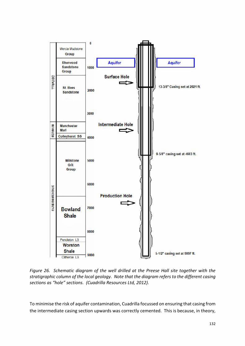
132
Figure 26. Schematic diagram of the well drilled at the Preese Hall site together with the stratigraphic column of the local geology. Note that the diagram refers to the different casing sections as “hole” sections. (Cuadrilla Resources Ltd, 2012).
To minimise the risk of aquifer contamination, Cuadrilla focussed on ensuring that casing from
the intermediate casing section upwards was correctly cemented. This is because, in theory,

133
if the installation of cement and casing down to the base of the intermediate casing is of high
enough standard, the risk of ground water contamination is minimised as the cement should
form a seal with the Manchester marl.
Cuadrilla put in place a number of quality control measures to ensure that the cement and
casing were correctly installed. A suite of tests were first carried out on the cement
components (dry cement and the mixing water), this allowed the cement composition to be
determined. Before pumping began, a casing calliper log was run. This detects any areas of
the borehole that have become enlarged during drilling. The results of the log allow the
volume of cement to be determined. Cuadrilla pumped excess cement down the wellbore as
a safety measure to ensure that sufficient cement returned to the surface. The hole was
cleaned after drilling and prior to installation of the casing.
The cement was mixed and pumped into the casing using a purpose built, fully automated
machine. It constantly monitors the cement density, rate of mixing, injection pressures and
injection rates. To complement this, samples of the cement were taken every few minutes
and the cement mix density was physically measured using mud balance scales (industry
standard). During the pumping, Cuadrilla employed “basic quality control procedures” but
fail to state exactly what these procedures are and what they examine.
After each section was filled with cement, the operation was shut down for at least 24 hours
to allow the cement to dry and harden. The desired amount of hardening was determined
using the samples of cement collected during the pumping stage. Once the cement has set
to sufficient compressive strength, so as to allow drilling to re-commence without the cement
fracturing, the operation was restarted. When drilling was restarted, the entirety of the new
section was not drilled. Instead, a further 20 ft. of wellbore was drilled and a FIT carried out.
During drilling at Preese Hall, the average mud weight used during the drilling was 9.2 ppg to
10.5 ppg for the surface and intermediate sections. FIT tests were conducted at 12.5 ppg and
14.5 ppg respectively indicating that there was a 25% and 40% safety margin for the surface
and intermediate case respectively. Cuadrilla considered that these safety margins together
with the measures in place to ensure a high standard cement job reduce the risk of leakage
from the well to an acceptable level.
Cuadrilla are required to conduct a CBL through the surface casing if they observe that either
cement did not circulate back to the surface, if there were any problems with the mixing
and / or pumping of the cement or if the FIT indicates leakage at pressures lower than those
expected in the reservoir. A CBL was not carried out for the surface and intermediate casing
sections in Cuadrilla's first two onshore wells as none of these three events took place. They
have, however, now committed to conducting bond logs as often as possible on any future
wells drilled by Cuadrilla.

134
Wellbore integrity was found to be poor in multiple areas in the bottom 100 ft. of the
production casing. This was attributed to areas where the borehole was wider than expected
due to breakout. Before remedial action was taken, the areas of poor bonding were tested
to establish whether the casing was actually leaking. To do this, a plug was inserted below
the area of poor bonding and a number of perforations are made at the bottom and top of
the area. Another plug with a tube through the centre was inserted at the top of the area of
interest (Figure 27). Water was pumped, at pressure, through the small tube into the area of
low bonding. If the pressure remains constant then the cement is deemed acceptable and
hydraulic fracturing continues. If, on the other hand, pressure drops then it is implied that
the water is entering into the cement, therefore, the cement is in need of repair. The repair
is carried out by replacing the circulated water with cement (Figure 27). Once the
re-cementing has taken place and has had time to harden, the plugs are removed and the
well cleaned. This remedial action was carried out successfully at the Preese Hall site.
Multiple stage hydraulic fracturing from the bottom up took place at Preese Hall. A total of
six fracturing stages were carried out. This involved installing perforations in the section of
interest. Fracturing takes place and a casing plug is inserted which effectively seals off the
previously fractured section. The process was then repeated in the next area of interest.

135
Figure 27. Schematic diagram of the remedial action taken to repair the cement around the production casing at the Preese Hall site. The dark grey represents were bonded cement, the light grey represents medium bonded cement and the brown represents areas of poor bonding. (From Cuadrilla Resources Ltd, 2012)
Fluid usage and waste disposal
During drilling, Cuadrilla published details of the three chemicals they were given permission
to use in the drilling fluid (Department of Energy and Climate Change, 2014e; Cuadrilla
Resources Ltd., 2015)

136
Polyacrylamide – used to reduce friction. 0.043% used in the drilling fluid. This is a
non-hazardous, non-toxic substance commonly used in cosmetics as well as drinking
and wastewater plants.
Dilute hydrochloric acid –used to dilute the drilling fluid.
Glutaraldehyde biocide – used to cleanse and remove bacteria from the water.
The composition of the fracturing fluid can be seen in Appendix 2. Of the three chemicals,
only polyacrylamide was used as the water supplied by United Utilities and was found to be
sufficiently pure. In addition to polyacrylamide, a small amount of salt, which acts as a tracer,
was added the fluid (Cuadrilla Resources Ltd., 2015). Based on the chemical content of the
fluid, the EA classified the fracturing fluid as being non-hazardous (Department of Energy and
Climate Change, 2014e; Cuadrilla Resources Ltd., 2015).
The flowback water was tested at the ground surface by both the EA and Cuadrilla and was
found to contain small amounts of NORM. The water underwent treatment and disposed
according to EA regulations in the EA approved Davyhulme water treatment plants (Cuadrilla
Resources Ltd., 2015).
Seismic activity at Preese Hall
Cuadrilla used of ‘Buried Array’, provided by MicroSeismic, and ‘Tiltmeter Array’ provided by
Pinnacle Technologies will be installed in 104 specially prepared holes around the site
extending to depths ranging from only 12 to 90 metres. During the series of seismic events
that took place at the Preese Hall site in April of 2011, 55 earthquakes were recorded over
the course of two days (Figure 28). Prior to injection, no seismic activity was recorded at the
site. This, in conjunction with the close temporal correlation of the events with the injection
of the fluids (approximately 10 hours difference) led to the inference that the seismicity was
induced and not natural (Davies et al., 2013). The reason for this lag is considered to be either
that it represents the time needed for the fluid pressure to be transferred to the fault or that
the fault has some inherent storage and fluid flow capacity (Davies et al., 2013).
Earthquakes resulting from hydraulic fracturing
In April of 2011 two earthquakes of magnitude 1.5 and 2.3 were detected in the Blackpool
area by the BGS. DECC halted all fracturing at the site and a number of reports were
commissioned as to the cause of the earthquakes (de Pater and Baisch, 2011; Green et al.,
2012; Styles and Baptie, 2012). It was determined that the hydraulic fracturing at the Preese
Hall site was the cause of the earthquakes, specifically, movement of the fracturing fluids
along a critically stressed fault. It was, however, noted that similar magnitude seismic activity
resulting from coal mining had been documented in the area (Styles and Baptie, 2012). These
events occurred at shallower depths than those associated with hydraulic fracturing whilst
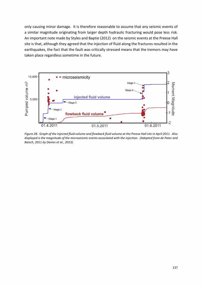
137
only causing minor damage. It is therefore reasonable to assume that any seismic events of
a similar magnitude originating from larger depth hydraulic fracturing would pose less risk.
An important note made by Styles and Baptie (2012) on the seismic events at the Preese Hall
site is that, although they agreed that the injection of fluid along the fractures resulted in the
earthquakes, the fact that the fault was critically stressed means that the tremors may have
taken place regardless sometime in the future.
Figure 28. Graph of the injected fluid volume and flowback fluid volume at the Preese Hall site in April 2011. Also displayed is the magnitude of the microseismic events associated with the injection. (Adapted from de Pater and Baisch, 2011 by Davies et al., 2013).
138
References Adam, R. and Kelsey, T. W. (2012). Pennsylvania dairy farms and Marcellus Shale, 2007–2010.
[Online] Available at :<http://pubs.cas.psu.edu/freepubs/pdfs/ee0020.pdf> [Accessed 20/03/2015]
Adams, M. B. (2011). Land application of hydrofracturing fluids damages a deciduous forest stand in West Virginia. Journal of Environmental Quality. 40(4), 1340-1344.
Adgate, J. L., Goldstein, B. D. and McKenzie, L. M. (2014). Potential public health hazards, exposures and health effects from unconventional natural gas development. Environmental Science & Technology. 48(15), 8307-8320.
Akcil, A. and Koldas, S. (2006). Acid Mine Drainage (AMD): causes, treatment and case studies. Journal of Cleaner Production. 14(12-13), 1139-1145.
Aksoy, N., Şimşek, C. and Gunduz, O. (2009). Groundwater contamination mechanism in a geothermal field: A case study of Balcova, Turkey. Journal of Contaminant Hydrology. 103(1-2), 13-28.
Alberta Energy Regulator. (2014). Flaring and Incineration. [online] Available at:<http://www.aer.ca/documents/enerfaqs/AER_EnerFAQs06_FlaringIncineration-Web.pdf> [Accessed 29/04/2015]
Allen, D. T., Torres, V. M., Thomas, J., Sullivan, D. W., Harrison, M., Hendler, A., Herndon, S. C., Kolb, C. E., Fraser, M. P., Hill, A. D., Lamb, B. K., Miskimins, J., Sawyer, R. F. and Seinfeld, J. H. (2013). Measurements of methane emissions at natural gas production sites in the United States. Proceedings of the National Academy of Sciences. 110(44), 17768-17773.
Almond, S., Clancy, S. A., Davies, R. J. and Worrall, F. (2014). The flux of radionuclides in flowback fluid from shale gas exploitation. Environmental Science and Pollution Research. 21(21), 12316-12324.
American Petroleum Institute. (2009). Environmental protection for onshore oil and gas production operations and leases; Recommended Practice 51R. Washington DC. [online] Available at:<https://www.gov.uk/government/uploads/system/uploads/attachment_data/file/291485/LIT_7311_514be9.pdf> [Accessed 30/04/2015]
Arabasz, W. J., Nava, S. J., McCarter, M. K., Pankow, K. L., Pechmann, J. C., Ake, J. and McGarr, A. (2005). Coal-mining seismicity and ground-shaking hazard: A case study in the Trail Mountain area, Emery County, Utah. Bulletin of the Seismological Society of America. 95(1), 18-30.
Babiker, I. S., Mohamed, M. A. A., Terao, H., Kato, K. and Ohta, K. (2004). Assessment of groundwater contamination by nitrate leaching from intensive vegetable cultivation using geographical information system. Environment International. 29(8), 1009-1017.
Bamberger, M. and Oswald, R. E. (2012). Impacts of gas drilling on human and animal health. New solutions: a journal of environmental and occupational health policy. 22(1), 51-77.
Barbot, E., Vidic, N. S., Gregory, K. B. and Vidic, R. D. (2013). Spatial and temporal correlation of water quality parameters of produced waters from Devonian-age shale following hydraulic fracturing. Environmental Science & Technology. 47(6), 2562-2569.
Barker, J. F., Barbash, J. E. and Labonte, M. (1988). Groundwater contamination at a landfill sited on fractured carbonate and shale. Journal of Contaminant Hydrology. 3(1), 1-25.
BC Oil and Gas Commission. (2011). Oil and Gas Commission Fact Sheet; Overview: Flaring, Incinerating and Venting. [Online] Available at :< https://www.bcogc.ca/node/11464/download> [Accessed 29/04/2015]
Bhuiyan, M. A. H., Islam, M. A., Dampare, S. B., Parvez, L. and Suzuki, S. (2010). Evaluation of hazardous metal pollution in irrigation and drinking water systems in the vicinity of a coal mine area of north-western Bangladesh. Journal of Hazardous Materials. 179(1-3), 1065-1077.
139
Bott, R. D. (2007). Flaring: Questions + Answers. [Online] Available at :<http://siteresources.worldbank.org/EXTGGFR/Resources/578068-1258067586081/FlaringQA.pdf> [Accessed 29/04/2015]
Boyer, E. W., Swistock, B. R., Clark, J., Madden, M. and Rizzo, D. E. (2012). The Impact of Marcellus Gas Drilling on Rural Drinking Water Supplies. pp. 23
British Geological Survey. (2014). New Ollerton Earthquake Activity. [Online] Available at :<http://www.earthquakes.bgs.ac.uk/earthquakes/recent_events/ollerton_earthquakes.html> [Accessed 25/04/2015]
British Geological Survey. (2015a). Lower Greensand/Kimmeridge and Ampthill Clay separation map. [Online] Available at :<http://www.bgs.ac.uk/research/groundwater/shaleGas/aquifersAndShales/maps/separationMaps/lg-ka.html> [Accessed 01/05/2015]
British Geological Survey. (2015b). Triassic Sandstone/Bowland and Craven Groups separation map. [Online] Available at :<http://www.bgs.ac.uk/research/groundwater/shaleGas/aquifersAndShales/maps/separationMaps/ts-bcg.html> [Accessed 01/05/2015]
Broderick, J., Anderson, K., Wood, R., Gilbert, P., Sharmina, M., Footitt, A., Glynn, S. and Nicholls, F. (2011). Shale gas: an updated assessment of environmental and climate change impacts. A report commissions by the Co-operative and undertaken by researchers at the Tyndall Centre, University of Manchester. [Online] Available at :<http://www.tyndall.ac.uk/sites/default/files/coop_shale_gas_report_update_v3.10.pdf> [Accessed 03/05/2015]
Broni-Bediako, E. and Amorin, R. (2010). Effects of drilling fluid exposure to oil and gas workers presented with major areas of exposure and exposure indicators. Research Journal of Applied Sciences, Engineering and Technology. 2(8), 710-719.
Broomfield, M. (2012). Support to the Identification of Potential Risks for the Environment and Human Health Arising from Hydrocarbons Operations Involving Hydraulic Fracturing in Europe. European Commission DG Environment publication 07.0307/ENV.C.1/2011/604781/ENV.F1. [Online] Available at :<http://ec.europa.eu/environment/integration/energy/pdf/fracking%20study.pdf> [Accessed 19/04/2015]
Broomfield, M. and Donovan, B. (2012). Monitoring and control of fugitive methane from unconventional gas operations. pp. 93
Bunch, A. G., Perry, C. S., Abraham, L., Wikoff, D. S., Tachovsky, J. A., Hixon, J. G., Urban, J. D., Harris, M. A. and Haws, L. C. (2014). Evaluation of impact of shale gas operations in the Barnett Shale region on volatile organic compounds in air and potential human health risks. Science of the Total Environment. 468-469, 832-842.
Carbon Capture & Storage Association. (2015). What is CSS? [Online] Available at :<http://www.ccsassociation.org/what-is-ccs/> [Accessed 10/03/2015]
Carey, J. W., Svec, R., Grigg, R., Zhang, J. and Crow, W. (2010). Experimental investigation of wellbore integrity and CO2-brine flow along the casing-cement microannulus. International Journal of Greenhouse Gas Control. 4(2), 272-282.
Chapman, E. C., Capo, R. C., Stewart, B. W., Kirby, C. S., Hammack, R. W., Schroeder, K. T. and Edenborn, H. M. (2012). Geochemical and strontium isotope characterization of produced waters from Marcellus Shale natural gas extraction. Environmental Science & Technology. 46(6), 3545-3553.
Chartered Institute of Water and Environmental Management. (2014). Shale Gas and Water. [Online] Available at :<http://www.ciwem.org/media/1023226/Shale%20Gas%20and%20Water%20WEB.pdf> [Accessed 03/05/2015]

140
Cherry, J., Ben-Eli, M., Bharadwaj, L., Chalaturnyk, R., Dusseault, M., Goldstein, B., Lacoursière, J.-P., Matthews, R., Mayer, B., Molson, J., Munkittrick, K., Oreskes, N., Parker, B. and Young, P. (2014). Environmental Impacts of Shale Gas Extraction in Canada; The Expert Panel on Harnessing Science and Technology to Understand the Environmental Impacts of Shale Gas Extraction. [Online] Available at :<http://www.scienceadvice.ca/uploads/eng/assessments%20and%20publications%20and%20news%20releases/shale%20gas/shalegas_fullreporten.pdf> [Accessed 20/04/2015]
Choi, Y.-S., Young, D., Nešić, S. and Gray, L. G. S. (2013). Wellbore integrity and corrosion of carbon steel in CO2 geologic storage environments: A literature review. International Journal of Greenhouse Gas Control. 16, Supplement 1, S70-S77.
Chowdhury, S., Champagne, P. and McLellan, P. J. (2010a). Factorial analysis of trihalomethanes formation in drinking water. Water Environment Research. 82(6), 556-566.
Chowdhury, S., Champagne, P. and McLellan, P. J. (2010b). Investigating effects of bromide ions on trihalomethanes and developing model for predicting bromodichloromethane in drinking water. Water Research. 44(7), 2349-2359.
Classic, K. (2013). Radiation Basics. [Online] Available at :<http://hps.org/publicinformation/ate/faqs/radiation.html> [Accessed 10/06/2015]
Colborn, T., Kwiatkowski, C., Schultz, K. and Bachran, M. (2011). Natural Gas Operations from a Public Health Perspective. Human and Ecological Risk Assessment: An International Journal. 17(5), 1039-1056.
Colorado Department of Public Health and Environment. (2009). Garfield County emissions inventory. Air Pollution Control Division. pp. 34
Colorado Department of Public Health and Environment. (2010). Public health implications of ambient air exposures as measured in rural and urban oil & gas development areas — an analysis of 2008 air sampling data. pp. 29
Coons, T. and Walker, R. (2008). Community health risk analysis of oil and gas industry impacts in Garfield County. pp. 227
Coussens, C. and Martinez, R. M. (2013). Roundtable on Environmental Health Sciences, Research, and Medicine, The Board on Population Health and Public Health Practice, and the Institute of Medicine. Health impact assessment of shale gas extraction: workshop summary. Washington, DC. pp. 116
Crook, R. (2006). Cementing. In: Mitchell, R. F. (Eds). Petroleum Engineering Handbook, Volume II: Drilling Engineering. Society of Petroleum Engineers, 369-431.
Cuadrilla Resources Ltd. (2012). Wellbore integrity - Cuadrilla Land Based Wells. [Online] Available at :<http://www.cuadrillaresources.com/what-we-do/drilling/> [Accessed 01/02/2015]
Cuadrilla Resources Ltd. (2015). Water Disposal. [Online] Available at :<http://www.cuadrillaresources.com/protecting-our-environment/water/water-disposal/> [Accessed 18/06/2015]
Cuadrilla Resources Ltd. (2015). Fracturing Fluid. [Online] Available at :<http://www.cuadrillaresources.com/what-we-do/hydraulic-fracturing/fracturing-fluid/> [Accessed 27/01/2015]
Darrah, T. H., Vengosh, A., Jackson, R. B., Warner, N. R. and Poreda, R. J. (2014). Noble gases identify the mechanisms of fugitive gas contamination in drinking-water wells overlying the Marcellus and Barnett Shales. Proceedings of the National Academy of Sciences. 111(39), 14076-14081.
Davies, R., Foulger, G., Bindley, A. and Styles, P. (2013). Induced seismicity and hydraulic fracturing for the recovery of hydrocarbons. Marine and Petroleum Geology. 45, 171-185.
Davies, R. J. (2011). Methane contamination of drinking water caused by hydraulic fracturing remains unproven. Proceedings of the National Academy of Sciences. 108(43), E871.
141
Davies, R. J., Almond, S., Ward, R. S., Jackson, R. B., Adams, C., Worrall, F., Herringshaw, L. G., Gluyas, J. G. and Whitehead, M. A. (2014). Oil and gas wells and their integrity: Implications for shale and unconventional resource exploitation. Marine and Petroleum Geology. 56, 239-254.
Davies, R. J., Mathias, S. A., Moss, J., Hustoft, S. and Newport, L. (2012). Hydraulic fractures: How far can they go? Marine and Petroleum Geology. 37(1), 1-6.
Davis, S. D. and Frohlich, C. (1993). Did (or will) fluid injection cause earthquakes? - Criteria for a rational assessment. Seismological Research Letters. 64(3-4), 207-224.
de Pater, C. J. and Baisch, S. (2011). Geomechanical Study of Bowland Shale Seismicity: Synthesis Report. pp. 57
Department of Energy and Climate Change. (2013). Onshore oil and gas exploration in the UK: regulation and best practice. pp. 49
Department of Energy and Climate Change. (2014a). Fracking UK shale: local air quality. pp. 6 Department of Energy and Climate Change. (2014b). Fracking UK shale: regulation and monitoring.
pp. 6 Department of Energy and Climate Change. (2014c). Fracking UK shale: safety from design to
decommissioning. pp. 6 Department of Energy and Climate Change. (2014d). Fracking UK shale: understanding earthquake
risk. pp. 6 Department of Energy and Climate Change. (2014e). Fracking UK shale: water. pp. 8 DiGiulio, D. C., Wilkin, R. T., Miller, C. and Oberly, G. (2011). DRAFT: Investigation of Ground Water
Contamination near Pavillion, Wyoming. pp. 43 Dixon, D. W. (2001). Radon exposures from the use of natural gas in buildings. Radiation Protection
Dosimetry. 97(3), 259-264. Dogdu, M. S. and Bayari, C. S. (2005). Environmental impact of geothermal fluids on surface water,
groundwater and streambed sediments in the Akarcay Basin, Turkey. Environmental Geology. 47(3), 325-340.
Down, A., Armes, M. and Jackson, R. B. (2012). Shale gas extraction in North Carolina: research recommendations and public health implications. Environmental Health Perspectives. 121(10), A292.
EGS Solutions. (2015). Microseismic Monitoring 101. [Online] Available at :< https://www.esgsolutions.com/technical-resources/microseismic-knowledgebase/microseismic-monitoring-101> [Accessed 19/06/2015]
Engelder, T. (2012). Capillary tension and imbibition sequester frack fluid in Marcellus gas shale. Proceedings of the National Academy of Sciences. 109(52), E3625.
Environment Agency. (2010). Guidance for monitoring enclosed landfill gas flares. [Online] Available at :< https://www.gov.uk/government/uploads/system/uploads/attachment_data/file/321610/LFTGN05.pdf> [Accessed 29/04/2015]
Environment Agency. (2011). Shale Gas. North West - Monitoring of Flowback water. [Online] Available at :<http://webarchive.nationalarchives.gov.uk/20140328084622/http://www.environment-agency.gov.uk/static/documents/Business/6th_Dec_-_Shale_gas_-_North_West_-_Monitoring_of_flowback_water_-_update_(3).pdf> [Accessed 18/06/2015]
Environment Agency. (2012a). Good practice for decommissioning redundant boreholes and wells. [Online] Available at :<http://webarchive.nationalarchives.gov.uk/20140328084622/http://cdn.environment-agency.gov.uk/LIT_6478_8cbe6f.pdf> [Accessed 22/04/2015]
Environment Agency. (2012b). Review of Assessment Procedures for Shale Gas Well Casing Installation. [Online] Available at :< https://www.gov.uk/government/uploads/system/uploads/attachment_data/file/291485/LIT_7311_514be9.pdf> [Accessed 25/03/2015]
142
Environment Agency. (2013). An Environmental Risk Assessment for shale gas exploratory operations in England: Version 1. pp. 32
Environmental Audit Committee. (2015). Environmental risks of fracking. Eighth Report of Session 2014–15. pp. 42
Esswein, E. J., Breitenstein, M., Snawder, J., Kiefer, M. and Sieber, W. K. (2013). Occupational exposures to respirable crystalline silica during hydraulic fracturing. Journal of Occupational and Environmental Hygiene. 10(7), 347-356.
Evans, K. F., Zappone, A., Kraft, T., Deichmann, N. and Moia, F. (2012). A survey of the induced seismic responses to fluid injection in geothermal and CO2 reservoirs in Europe. Geothermics. 41, 30-54.
Finkel, M. L. and Hays, J. (2013). The implications of unconventional drilling for natural gas: A global public health concern. Public health. 127(10), 889-893.
Finkel, M. L., Hays, J. and Law, A. (2013a). Modern Natural Gas Development and Harm to Health: The Need for Proactive Public Health Policies. ISRN Public Health. 2013, 1-5.
Finkel, M. L., Selegean, J., Hays, J. and Kondamudi, N. (2013b). Marcellus Shale drilling's impact on the dairy industry in Pennsylvania: a descriptive report. New solutions: a journal of environmental and occupational health policy. 23(1), 189-201.
Fletcher, J. B. and McGarr, A. (2005). Moment tensor inversion of ground motion from mining-induced earthquakes, Trail Mountain, Utah. Bulletin of the Seismological Society of America. 95(1), 48-57.
Flewelling, S. A., Tymchak, M. P. and Warpinski, N. (2013). Hydraulic fracture height limits and fault interactions in tight oil and gas formations. Geophysical Research Letters. 40(14), 3602-3606.
Frac Focus. (2015a). Hydraulic Fracturing: The Process. [online] Available at:<https://fracfocus.org/hydraulic-fracturing-how-it-works/hydraulic-fracturing-process> [Accessed 02/04/2015]
Frac Focus. (2015b). Why are chemcials used? [online] Available at:<https://www.fracfocus.org/chemical-use/why-chemicals-are-used> [Accessed 06/01/2015]
Friends of the Earth. (2005). Gas Flaring in Nigeria. [online] Available at:<http://www.foe.co.uk/sites/default/files/downloads/gas_flaring_nigeria.pdf> [Accessed 18/06/2015]
Fryzek, J., Pastula, S., Jiang, X. and Garabrant, D. H. (2013). Childhood Cancer Incidence in Pennsylvania Counties in Relation to Living in Counties With Hydraulic Fracturing Sites. Journal of Occupational and Environmental Medicine. 55(7), 796-801.
Gee, G. C. and Payne-Sturges, D. C. (2004). Environmental Health Disparities: A Framework Integrating Psychosocial and Environmental Concepts. Environmental Health Perspectives. 112(17), 1645-1653.
Gibson, J. (2013). Summary Report of Review of Flare and Vent Gas Emissions Monitoring and Reporting Methods. A Report for National Measurment Office. pp. 26
Godwin, K. S., Hafner, S. D. and Buff, M. F. (2003). Long-term trends in sodium and chloride in the Mohawk River, New York: the effect of fifty years of road-salt application. Environmental Pollution. 124(2), 273-281.
Goldstein, B. D. and Malone, S. (2013). Obfuscation Does Not Provide Comfort: Response to the Article by Fryzek et al on Hydraulic Fracturing and Childhood Cancer. Journal of Occupational and Environmental Medicine. 55(11), 1376-1378.
Gordalla, B. C., Ewers, U. and Frimmel, F. H. (2013). Hydraulic fracturing: a toxicological threat for groundwater and drinking-water? Environmental Earth Sciences. 70(8), 3875-3893.
Graham, J., Irving, J., Tang, X., Sellers, S., Crisp, J., Horwitz, D., Muehlenbachs, L., Krupnick, A. and Carey, D. (2015). Increased traffic accident rates associated with shale gas drilling in Pennsylvania. Accident Analysis & Prevention. 74, 203-209.

143
Granberg, A. (2015). What Is Hydraulic Fracturing? [online] Available at:<http://www.propublica.org/special/hydraulic-fracturing-national> [Accessed 02/02/2015]
Green, C. A., Styles, P. and Baptie, B. (2012). Preese Hall shale gas fracturing: Review and recommendations for induced esismic mitigation. pp. 26
Halliburton. (2006a). Cementing: Bow-Spring Centralizers. [online] Available at:<http://www.halliburton.com/public/cem/contents/Data_Sheets/web/H/H05051-A4.pdf> [Accessed 27/03/2015]
Halliburton. (2006b). Cementing: Rigid Centralizers. [online] Available at:<http://www.halliburton.com/public/cem/contents/data_sheets/web/h/h05055.pdf> [Accessed 27/03/2015]
Halliburton. (2011). Microseismic Events. How Big Are These Microseismic Events? [online] Available at:<http://www.halliburton.com/public/pinnacle/contents/Data_Sheets/web/H08325.pdf> [Accessed 02/04/2015]
Hammack, R., Harbert, W., Sharma, S., Stewart, B., Capo, R., Wall, A., Wells, A., Diehl, R., Sams, J. and Veloski, G. (2014). An Evaluation of Fracture Growth and Gas/Fluid Migration as Horizontal Marcellus Shale Gas Wells are Hydraulically Fractured in Greene County, Pennsylvania; NETL-TRS-3-2014; EPAct Technical Report Series; U.S. Department of Energy, National Energy Technology Laboratory: Pittsburgh, PA. pp. 76
Healey, D. (2012). Hydraulic Fracturing or ‘Fracking’: A Short Summary of Current Knowledge and Potential Environmental Impacts. A Small Scale Study for the Environmental Protection Agency (Ireland) under the Science, Technology, Research & Innovation for the Environment (STRIVE) Programme 2007 – 2013. pp. 26
Health and Safety Executive. (2004). The selection and use of flammable gas detectors. pp. 16 Hill, E. L. (2013). Shale gas development and infant health: Evidence from Pennsylvania. [online]
Available at:<http://dyson.cornell.edu/research/researchpdf/wp/2012/Cornell-Dysonwp1212.pdf.> [Accessed 09/02/2015/
Hladik, M. L., Focazio, M. J. and Engle, M. (2014). Discharges of produced waters from oil and gas extraction via wastewater treatment plants are sources of disinfection by-products to receiving streams. Science of The Total Environment. 466-467(0), 1085-1093.
Holditch, S. A. (2006). Hydraulic fracturing. In: Clegg, D. C. (Eds). Petroleum Engineering Handbook, Volume IV: Production Operations Engineering. Society of Petroleum Engineers, 323-366.
Holland, A. A. (2014). Imaging Time Dependent Crustal Deformation Using GPS Geodesy and Induced Seismicity, Stress and Optimal Fault Orientations in the North American Mid-Continent. Graduate Thesis. University of Arizona. [online] Available at:<http://pqdtopen.proquest.com/doc/1614168780.html?FMT=AI> [Accessed 24/04/2015]
Horleston, A., Stork, A., Verdon, J., Baird, A., Wookey, J. and Kendall, M. (2013). Seismic Monitoring of Drilling Operations In Balcombe, West Sussex. [online] Available at:<http://www1.gly.bris.ac.uk/BUMPS/PDFS/BristolBalcombeReport2013.pdf> [Accessed 24/04/2015]
House of Commons. (2011). House of Commons Energy and Climate Change Committee. Shale Gas: Fifth Report of Session 2010–12; Seventh Special Report of Session 2010–12. [online] Available at:<https://www.gov.uk/government/uploads/system/uploads/attachment_data/file/79188/shalegas-govresp.pdf> [Accessed 03/05/2015]
House of Commons Energy and Climate Change Committee. (2011). Shale Gas Fifth Report of Session 2010–12. Volume I: Report, together with formal minutes, oral and written evidence pp. 65
Hubbert, M. K. and Willis, D. G. (1972). Mechanics of hydraulic fracturing(Eds). M 18: Underground Waste Management and Environmental Implications, 239-257.
Ingraffea, A. R. (2012). Fluid migration mechanisms due to faulty well design and/or construction: An overview and recent experiences in the Pennsylvania Marcellus play. pp. 10
144
Ingraffea, A. R., Wells, M. T., Santoro, R. L. and Shonkoff, S. B. C. (2014). Assessment and risk analysis of casing and cement impairment in oil and gas wells in Pennsylvania, 2000–2012. Proceedings of the National Academy of Sciences. 111(30), 10955-10960.
Institute of Medicine of the National Academies Board on Population Health and Public Health Practice Roundtable on Environmental Health Sciences Research and Medicine (IOM). (2014). Health Impact Assessment of Shale Gas Extraction: Workshop Summary. [online] Available at:<http://www.nap.edu/catalog/18376/health-impact-assessment-of-shale-gas-extraction-workshop-summary> [Accessed 19/04/2015]
IPIECA. (2013). Green Completions. [online] Available at:<http://www.ipieca.org/energyefficiency/solutions/78161> [Accessed 26/01/2015]
Jackson, R. B. (2014). The integrity of oil and gas wells. Proceedings of the National Academy of Sciences. 111(30), 10902-10903.
Jackson, R. B., Vengosh, A., Darrah, T. H., Warner, N. R., Down, A., Poreda, R. J., Osborn, S. G., Zhao, K. and Karr, J. D. (2013). Increased stray gas abundance in a subset of drinking water wells near Marcellus shale gas extraction. Proceedings of the National Academy of Sciences. 110(28), 11250-11255.
Johnson, D. B. and Hallberg, K. B. (2005). Acid mine drainage remediation options: a review. Science of The Total Environment. 338(1-2), 3-14.
Johnson, R. (1973). Assessment of Potential Radiological Health Effects from Radon in Natural Gas. Report for US Environmental Protection Agency. United States Environmental Protection Agency. [online] Available at:<http://rwma.com/Johnson%20et%20al.,%201973.pdf> [Accessed 02/05/2015]
Kaktins, N. M. (2011). Drilling the Marcellus shale for natural gas: environmental health issues for nursing. The Pennsylvania nurse. 66(1), 4.
Kang, M., Kanno, C. M., Reid, M. C., Zhang, X., Mauzerall, D. L., Celia, M. A., Chen, Y. and Onstott, T. C. (2014). Direct measurements of methane emissions from abandoned oil and gas wells in Pennsylvania. Proceedings of the National Academy of Sciences. 111(51), 18173-18177.
Kargbo, D. M., Wilhelm, R. G. and Campbell, D. J. (2010). Natural Gas Plays in the Marcellus Shale: Challenges and Potential Opportunities. Environmental Science & Technology. 44(15), 5679-5684.
Kassotis, C. D., Tillitt, D. E., Davis, J. W., Hormann, A. M. and Nagel, S. C. (2014). Estrogen and androgen receptor activities of hydraulic fracturing chemicals and surface and ground water in a drilling-dense region. Endocrinology. 155(3), 897-907.
Kemball-Cook, S., Bar-Ilan, A., Grant, J., Parker, L., Jung, J., Santamaria, W., Mathews, J. and Yarwood, G. (2010). Ozone Impacts of Natural Gas Development in the Haynesville Shale. Environmental Science & Technology. 44(24), 9357-9363.
Kibble, A., Cabianca, T., Daraktchieva, Z., Gooding, T., Smithard, J., Kowalczyk, G., McColl, N. P., Singh, M., Mitchem, L., Lamb, P., Vardoulakis, S. and Kamanyire, R. (2013). Public Health England: Review of the Potential Public Health Impacts of Exposures to Chemical and Radioactive Pollutants as a Result of the Shale Gas Extraction Process. pp. 52
King, G. E. (1996). An Introduction to the Basics of Well Completions, Stimulations and Workovers; Chapter 3: Cement. 2nd ed.
King, G. E. and King, D. E. (2013). Environmental risk arising from well-construction failure - Differences between barrier and well failure, and estimates of failure frequency across common well types, locations, and well age. SPE Production & Operations. 28(4), 323-344.
Kinik, K. and Wojtanowicz, A. K. (2011). Identifying environmental risk of sustained casing pressure. Society of Petroleum Engineers Conference Paper. SPE-143713-MS.
Kondash, A. J., Warner, N. R., Lahav, O. and Vengosh, A. (2014). Radium and barium removal through blending hydraulic fracturing fluids with acid mine drainage. Environmental Science & Technology. 48(2), 1334-1342.
145
La Plata County. (2002). La Plata County impact report. [online] Available at:<http://www.co.laplata.co.us/departments_elected_officials/planning/natural_resources_oil_gas/impact_report> [Accessed 20/03/2015]
Laney, A. S. and Weissman, D. N. (2012). The Classic Pneumoconioses: New Epidemiological and Laboratory Observations. Clinics in Chest Medicine. 33(4), 745-758.
Levallois, P., Thériault, M., Rouffignat, J., Tessier, S., Landry, R., Ayotte, P., Girard, M., Gingras, S., Gauvin, D. and Chiasson, C. (1998). Groundwater contamination by nitrates associated with intensive potato culture in Québec. Science of The Total Environment. 217(1-2), 91-101.
Lock, K. (2000). Health impact assessment. BMJ : British Medical Journal. 320(7246), 1395-1398. Logan, J., Heath, G., Macknick, J., Paranhos, E., Boyd, W. and Carlson, K. (2012). The Joint Institute for
Strategic Energy Analysis Report. Natural Gas and the Transformation of the U.S. Energy Sector: Electricity. pp. 240
Løseth, H., Wensaas, L., Arntsen, B., Hanken, N.-M., Basire, C. and Graue, K. (2011). 1000 m long gas blow-out pipes. Marine and Petroleum Geology. 28(5), 1047-1060.
Macey, G., Breech, R., Chernaik, M., Cox, C., Larson, D., Thomas, D. and Carpenter, D. (2014). Air concentrations of volatile compounds near oil and gas production: a community-based exploratory study. Environmental Health. 13(1), 82.
MacKay, D. J. C. and Stone, T. J. (2013). Potential Greenhouse Gas Emissions Associated with Shale Gas Extraction and Use. pp. 39
Massachusetts Institute of Technology. (2011). Study on the Future of Natural Gas. MIT Energy Initiative. [online] Available at:<http://mitei.mit.edu/publications/reports-studies/future-natural-gas> [Accessed 21/04/2015]
McCoy, D. and Saunders, P. (2015). Health and Fracking: The impact and opportunity costs. pp. 32 McCrawley, M. (2012). Air, Noise, and Light Monitoring Plan for Assessing Environmental Impacts of
Horizontal Gas Well Drilling Operations (ETD-10 Project), West Virginia University School of Public Health, Morgantown, WV. [online] Available at:<http://www.dep.wv.gov/oil-and-gas/Horizontal-Permits/legislativestudies/Documents/WVU%20Final%20Air%20Noise%20Light%20Protocol.pdf> [Accessed 10/04/2015]
McCrawley, M. (2013). Air, Noise, and Light Monitoring Results for Assessing Environmental Impacts of Horizontal Gas Well Drilling Operations. West Virginia University School of Public Health, Morgantown, WV. [online] Available at:<http://wvwri.org/wp-content/uploads/2013/10/a-n-l-final-report-for-web.pdf> [Accessed 10/04/2015]
McGarr, A. and Fletcher, J. B. (2005). Development of ground-motion prediction equations relevant to shallow mining-induced seismicity in the Trail Mountain Area, Emery County, Utah. Bulletin of the Seismological Society of America. 95(1), 31-47.
McKenzie, L. M., Guo, R., Witter, R. Z., Savitz, D. A., Newman, L. S. and Adgate, J. L. (2014). Birth outcomes and maternal residential proximity to natural gas development in rural Colorado. Environ Health Perspect. 122(4), 412-7.
McKenzie, L. M., Witter, R. Z., Newman, L. S. and Adgate, J. L. (2012). Human health risk assessment of air emissions from development of unconventional natural gas resources. Science of The Total Environment. 424, 79-87.
Microseismic. (2014). Trusted Data Acquisition Methods: Enhacning Reservoir Completions Techniques and Production. [online] Available at:<http://www.microseismic.com/brochures/MSI_Brochure_DataAcquisition.pdf> [Accessed 19/06/2015]
Miyazaki, B. (2009). Well integrity: An overlooked source of risk and liability for underground natural gas storage. Lessons learned from incidents in the USA. Geological Society, London, Special Publications. 313(1), 163-172.

146
Molofsky, L. J., Connor, J. A., Farhat, S. K., Wylie, A. S. and Wagner, T. (2011). Methane in Pennsylvania water wells unrelated to Marcellus shale fracturing. Oil and Gas Journal. 109(49), 54-67.
Molofsky, L. J., Connor, J. A., Wylie, A. S., Wagner, T. and Farhat, S. K. (2013). Evaluation of Methane Sources in Groundwater in Northeastern Pennsylvania. Groundwater. 51(3), 333-349.
Monteiro Santos, F. A., Mateus, A., Figueiras, J. and Gonçalves, M. A. (2006). Mapping groundwater contamination around a landfill facility using the VLF-EM method - A case study. Journal of Applied Geophysics. 60(2), 115-125.
Montgomery, C. (2013). Fracturing Fluids. In: Bunger, A. P., McLennan, J. & Jeffrey, R. (Eds). Effective and Sustainable Hydraulic Fracturing, 1-24.
Mor, S., Ravindra, K., Dahiya, R. P. and Chandra, A. (2006). Leachate Characterization and Assessment of Groundwater Pollution Near Municipal Solid Waste Landfill Site. Environmental Monitoring and Assessment. 118(1-3), 435-456.
Murat Özler, H. (2000). Hydrogeology and geochemistry in the Curuksu (Denizli) hydrothermal field, western Turkey. Environmental Geology. 39(10), 1169-1180.
Myers, T. (2012). Potential contaminant pathways from hydraulically fractured shale to aquifers. Groundwater. 50(6), 872-882.
National Commission on the BP Deepwater Horizon Oil Spill and Offshore Drilling. (2011). Macondo: The Gulf Oil Disaster; Chief Counsel’s Report. Chapter 4.6. [online] Available at:<http://www.eoearth.org/files/164401_164500/164441/c21462-214_ccr_chp_4-6_negative_pressure_test.pdf> [Accessed 18/06/2015]
National Energy Technology Laboratory. (2014). Development of Nanoparticle-Stabilized Foams To Improve Performance of Water-less Hydraulic Fracturing. [online] Available at:<http://www.netl.doe.gov/research/oil-and-gas/project-summaries/enhanced-oil-recovery/fe0013723-UTA> [Accessed 28/04/2015]
National Energy Technology Laboratory. (2015a). Development and Field Testing Novel Natural Gas Surface Process Equipment for Replacement of Water as Primary Hydraulic Fracturing Fluid. [online] Available at:<http://www.netl.doe.gov/research/oil-and-gas/project-summaries/unconventional-resources/fe0024314-swri> [Accessed 28/04/2015]
National Energy Technology Laboratory. (2015b). Methods to Enhance Wellbore Cement Integrity with Microbially-Induced Calcite Precipitation (MICP). [online] Available at:<http://www.netl.doe.gov/research/oil-and-gas/project-summaries/unconventional-resources/fe0024296-msu> [Accessed 28/04/2015]
National Energy Technology Laboratory. (2015c). “Nanite” for Better Well-Bore Integrity and Zonal Isolation. [online] Available at:<http://www.netl.doe.gov/research/oil-and-gas/project-summaries/natural-gas-resources/fe0014144-Oceanit> [Accessed 28/04/2015]
National Energy Technology Laboratory. (2015d). nXis Well Integrity Inspection in Unconventional Wells. [online] Available at:<http://www.netl.doe.gov/research/oil-and-gas/project-summaries/unconventional-resources/fe0024293-geglobal> [Accessed 28/04/2015]
National Energy Technology Laboratory. (2015e). Unconventional Resources. [online] Available at:<http://www.netl.doe.gov/research/oil-and-gas/project-summaries/unconventional-resources> [Accessed 28/04/2015]
National Institute of Environmental Health Sciences. (2015). Endocrine Disruptors. [online] Available at:<http://www.niehs.nih.gov/health/topics/agents/endocrine/> [Accessed 15/06/2015]
Natural Gas STAR Partners. (2006a). Optimize Glycol Circulation And Install Flash Tank Separators In Glycol Dehydrators pp. 10
Natural Gas STAR Partners. (2006b). Options For Reducing Methane Emissions From Pneumatic Devices In The Natural Gas Industry pp. 12
Natural Gas STAR Partners. (2006c). Replacing Glycol Dehydrators With Desiccant Dehydrators pp. 14 New York State Department of Environmental Conservation. (2011). Revised Draft SGEIS on the Oil,
Gas and Solution Mining Regulatory Program (September 2011). Well Permit Issuance for

147
Horizontal Drilling and High-Volume Hydraulic Fracturing in the Marcellus Shale and Other Low-Permeability Gas Reservoirs. pp. 1537
New York State Department of Health. (2014). A Public Health Review of High Volume Hydraulic Fracturing for Shale Gas Development. pp. 176
Neymeyer, A., Williams, R. T. and Younger, P. L. (2007). Migration of polluted mine water in a public supply aquifer. Quarterly Journal of Engineering Geology and Hydrogeology. 40(1), 75-84.
Nolen-Hoeksema, R. (2013). Elements of hydraulic fracturing. Oilfield Review. 25(2), 51-52. NTC Consultants. (2011). Impacts on community character of horizontal drilling and high volume
hydraulic fracturing in Marcellus shale and other low-permeability gas reservoirs. Final Report. Prepared for the New York State Energy Research and Development Authority. pp. 45
Oil and Gas UK. (2009). Guidance on suspension and abandonment of wells/ North Sea well abandonment study. OP006. Issue 3. London: Oil and Gas UK.
Oil and Gas UK. (2012). Well integrity guidelines. [online] Available at:<http://www.oilandgasuk.co.uk/cmsfiles/modules/publications/pdfs/OP069.pdf> [Accessed 10/06/2015]
Osborn, S. G., Vengosh, A., Warner, N. R. and Jackson, R. B. (2011). Methane contamination of drinking water accompanying gas-well drilling and hydraulic fracturing. Proceedings of the National Academy of Sciences. 108(20), 8172-8176.
OSPAR Commission. (2012). Discharges, spills and emissions from offshore oil and gas installations in 2010. pp. 48
Otton, J. K. (1992). Radon in soil gas and soil radioactivity in Prince George's County. [online] Available at:<http://pubs.usgs.gov/of/1992/0011/report.pdf> [Accessed 02/05/2015]
Ovuakporaye, S. I., Aloamaka, C. P., Ojieh, A. E., Ejebe, D. E. and Mordi, J. C. (2012). Effects of gas flaring on lung function among residents in gas flaring community in Delta State, Nigeria. Research Journal of Environmental and Earth Sciences. 4(5), 525-528.
Papoulias, D. M. and Velasco, A. L. (2013). Histopathological analysis of fish from Acorn Fork Creek, Kentucky exposed to hydraulic fracturing fluid releases. Southeastern Naturalist. 12(4).
Penning, T. M., Breysse, P. N., Gray, K., Howarth, M. and Yan, B. (2014). Environmental health research recommendations from the inter-environmental health sciences core center working group on unconventional natural gas drilling operations. Environmental Health Perspectives. 122(11), 1155.
Pennsylvania Department of Environmental Protection. (2012). DEP Conducting Long-Term Marcellus Shale Air Monitoring Study in Southwestern Pennsylvania. [online] Available at:<http://www.portal.state.pa.us/portal/server.pt/community/oil_and_gas_related_topics/20349/air/986695> [Accessed 14/04/2015]
Perma-Fix Environmental Services Inc. (2015). Technologically Enhanced Naturally Occurring Radioactive Materials (TENORM) Study Report: A report prepared for teh Pennsylvania Department of Environmental Protection. [online] Available at:<http://www.elibrary.dep.state.pa.us/dsweb/Get/Document-105822/PA-DEP-TENORM-Study_Report_Rev._0_01-15-2015.pdf> [Accessed 10/04/2015]
Perry, S. L. (2012). Environmental reviews and case studies: Addressing the societal costs of unconventional oil and gas exploration and production: A framework for evaluating short-term, future, and cumulative risks and uncertainties of hydrofracking. Environmental Practice. 14(4), 352-365.
Perry, S. L. (2013). Using ethnography to monitor the community health implications of onshore unconventional oil and gas developments: examples from Pennsylvania's Marcellus Shale. New solutions: a journal of environmental and occupational health policy. 23(1), 33-53.
Pétron, G., Frost, G., Miller, B. R., Hirsch, A. I., Montzka, S. A., Karion, A., Trainer, M., Sweeney, C., Andrews, A. E., Miller, L., Kofler, J., Bar-Ilan, A., Dlugokencky, E. J., Patrick, L., Moore, C. T., Ryerson, T. B., Siso, C., Kolodzey, W., Lang, P. M., Conway, T., Novelli, P., Masarie, K., Hall, B., Guenther, D., Kitzis, D., Miller, J., Welsh, D., Wolfe, D., Neff, W. and Tans, P. C. D. (2012).

148
Hydrocarbon emissions characterization in the Colorado Front Range: A pilot study. Journal of Geophysical Research: Atmospheres. 117(D4), n/a-n/a.
PetroWiki. (2014a). Cement bond logs. [online] Available at:<http://petrowiki.org/Cement_bond_logs#Noteworthy_papers_in_OnePetro> [Accessed 12/06/2015]
PetroWiki. (2014b). Cement composition and classification. [online] Available at:<http://petrowiki.org/Cement_composition_and_classification#API_classifications> [Accessed 25/03/2015]
PetroWiki. (2014c). Cementing hardware. [online] Available at:<http://petrowiki.org/Cementing_hardware> [Accessed 27/03/2015]
Petrowiki. (2015). Gas lift. [online] Available at:<http://petrowiki.org/Gas_lift> [Accessed 29/04/2015]
Rabinowitz, P. M., Slizovskiy, I. B., Lamers, V., Trufan, S. J., Holford, T. R., Dziura, J. D., Peduzzi, P. N., Kane, M. J., Reif, J. S. and Weiss, T. R. (2015). Proximity to natural gas wells and reported health status: Results of a household survey in Washington County, Pennsylvania. Environmental Health Perspectives. 123(1), 21-26.
Rassenfoss, S. (2011). From flowback to fracturing: water recycling grows in the Marcellus shale. Journal of Petroleum Technology. 63(7), 48-51.
ReFINE. (2014). How radioactive is fracking flowback water? DEI Briefing Note No. 905: Autumn 2014. [online] Available at:<https://www.dur.ac.uk/resources/refine/NORMRB.pdf> [Accessed 27/04/2015]
Research Partnership to Secure Energy for America. (2013). Development of Non-Contaminating Cryogenic Fracturing Technology for Shale and Tight Gas Reservoirs. [online] Available at:<http://www.rpsea.org/media/files/project/3d9af270/10122-20-Development_Non-Contaminating_Cryogenic_Fracturing_Technology_Shale_Tight_Gas_Reservoirs-06-17-13.pdf> [Accessed
Research Partnership to Secure Energy for America. (2014). Prevention and Remediation of Sustained Casing Pressure and other Isolation Breaches. [online] Available at:<http://www.rpsea.org/media/files/project/b0d66da0/11122-42-PFS-Prevention_Remediation_Sustained_Casing_Pressure_Isolation_Breaches-03-19-14.pdf> [Accessed
Research Triangle Environmental Health Collaborative. (2013). Shale Gas Extraction in North Carolina: Public Health Implications. [online] Available at:<http://environmentalhealthcollaborative.org/images/2012SummitWorkProduct.pdf> [Accessed 19/04/2015]
Resnikoff, M. (2012). Radon in Natural Gas from Marcellus Shale. [online] Available at:<http://rwma.com/Marcellus%20Radon-%20Ethics.pdf> [Accessed 02/05/2015]
Resnikoff, M., Alexandrova, E. and Travers, J. (2010). Radioactivity in Marcellus Shale Report prepared for Residents for the Preservation of Lowman and Chemung (RFPLC) [online] Available at:<http://energy.wilkes.edu/PDFFiles/Library/Marcellus%20Shale%20Radioactivity%20Report%205-18-2010.pdf> [Accessed
Rich, A., Grover, J. P. and Sattler, M. L. (2014). An exploratory study of air emissions associated with shale gas development and production in the Barnett Shale. Journal of the Air & Waste Management Association. 64(1), 61-72.
RKI Instruments. (2014). What is %LEL and %UEL. [online] Available at:<http://rkiinstruments.com/pages/faq/What_is_LEL_UEL.htm> [Accessed 18/03/2015]
Rowan, E. L. and Kraemer, T. F. (2012). Radon-222 Content of Natural Gas Samples from Upper and Middle Devonian Sandstone and Shale Reservoirs in Pennsylvania: Preliminary Data. US Geological Survey Open-file Report 2012–1159. [online] Available at:<http://pubs.usgs.gov/of/2012/1159/ofr2012-1159.pdf> [Accessed 02/05/2015]

149
Roy, A. A., Adams, P. J. and Robinson, A. L. (2014). Air pollutant emissions from the development, production, and processing of Marcellus Shale natural gas. Journal of the Air & Waste Management Association. 64(1), 19-37.
Saberi, P. (2013). Navigating medical issues in shale territory. New solutions: a journal of environmental and occupational health policy. 23(1), 209-221.
Saiers, J. E. and Barth, E. (2012). Comment on "Potential contaminant pathways from hydraulically fractured shale aquifers". Groundwater. 50(6), 826-828.
Searl, A. and Galea, K. S. (2011). Toxicological review of the possible effects associated with inhalation and dermal exposure to drilling fluid production stream. pp. 84
Shariq, L. (2013). Uncertainties associated with the reuse of treated hydraulic fracturing wastewater for crop irrigation. Environmental Science & Technology. 47(6), 2435-2436.
Sherar, B. W. A., Power, I. M., Keech, P. G., Mitlin, S., Southam, G. and Shoesmith, D. W. (2011). Characterizing the effect of carbon steel exposure in sulfide containing solutions to microbially induced corrosion. Corrosion Science. 53(3), 955-960.
Shonkoff, S. B. C., Hayes, J. and Finkel, M. L. (2014). Environmental public health dimensions of shale and tight gas development. Environmental Health Perspectives. 122(8), 787-795.
Singh, R. P. and Yadav, R. N. (1995). Prediction of subsidence due to coal mining in Raniganj coalfield, West Bengal, India. Engineering Geology. 39(1), 103-111.
Skoumal, R. J., Brudzinski, M. R. and Currie, B. S. (2015). Earthquakes induced by hydraulic fracturing in Poland Township, Ohio. Bulletin of the Seismological Society of America.
Sperger, C., Cook, K. and Klemow, K. (2012). Does Marcellus Shale pose a radioactivity risk? Institute for Energy and Environmental Research of Northeastern Pennsylvania Clearinghouse. [online] Available at:<http://energy.wilkes.edu/pages/184.asp> [Accessed 10/06/2015]
Stamford, L. and Azapagic, A. (2014). Life cycle environmental impacts of UK shale gas. Applied Energy. 134, 506-518.
States, S., Cyprych, G., Stoner, M., Wydra, F., Kuchta, J., Monnell, J. and Casson, L. (2013). Marcellus Shale drilling and brominated THMs in Pittsburgh, Pa., drinking water. Journal-American Water Works Association. 105(8), E432-E448.
Stedman, R. C., Jacquet, J. B., Filteau, M. R., Willits, F. K., Brasier, K. J. and McLaughlin, D. K. (2012). Environmental reviews and case studies: Marcellus shale gas development and new boomtown research: Views of New York and Pennsylvania residents. Environmental Practice. 14(4), 382-393.
Steinzor, N., Subra, W. and Sumi, L. (2013). Investigating links between shale gas development and health impacts through a community survey project in Pennsylvania. New solutions: a journal of environmental and occupational health policy. 23(1), 55-83.
Steinzor, N., Subra, W. and Sumim, L. (2012). Gas Patch Roulette: How Shale Gas Development Risks Public Health in Pennsylvania. . pp. 51
STUK - Radiation and Nuclear Safety Authority. (2012). Some examples of radiation doses. [online] Available at:<http://www.stuk.fi/sateilyvaara/en_GB/esim_annos/> [Accessed 15/06/2015]
Styles, P. and Baptie, B. (2012). Briefing note on induced seismicity in the UK and its relevance to hydraulic stimulation for exploration for shale gas. pp. 12
Subra, W. (2009). Results of health survey of current and former DISH/Clark, Texas residents. Earthworks. pp. 17
Subra, W. (2010). Community health survey results, Pavillion, Wyoming residents. Earthworks. pp. 13 Talabani, S., Atlas, B., Al-Khatiri, M. B. and Islam, M. R. (2000). An alternate approach to downhole
corrosion mitigation. Journal of Petroleum Science and Engineering. 26(1-4), 41-48. Texas Department of State Health Services. (2010a). DISH, Texas exposure investigation Dish, Denton
County, Texas. pp. 38 Texas Department of State Health Services. (2010b). Summary of investigation into the occurrence of
cancer zip codes 75022 and 75028, Flower Mound, Denton County, Texas 1998–2007, 2007–2009. pp. 17

150
Texas Department of State Health Services. (2011). Updated summary report of Texas Department of State Health Services investigation of specific cancer occurrences within zip codes 75022 an 75028, Flower Mound, Denton County, Texas covering 1999–2008, 2008–2010. pp. 17
The Groundwater Foundation. (2015). Potential Threats to Our Groundwater. [online] Available at:<http://www.groundwater.org/get-informed/groundwater/contamination.html> [Accessed 10/03/2015]
The Royal Society and the Royal Academy of Engineering. (2012). Shale gas extraction in the UK: a review of hydraulic fracturing. pp. 76
United Kingdom Onshore Operators Group. (2013a). Fact Sheet: Development and the Drilling Process. [online] Available at:<http://www.ukoog.org.uk/onshore-extraction/stages-of-development> [Accessed 06/01/2015]
United Kingdom Onshore Operators Group. (2013b). Water UK and UKOOG to work together to minimise the impact of shale gas development on water resources in the UK. [online] Available at:<http://www.ukoog.org.uk/about-ukoog/press-releases/63-water-uk-and-ukoog-to-work-together-to-minimise-the-impact-of-shale-gas-development-on-water-resources-in-the-uk> [Accessed 02/05/2015]
United Kingdom Onshore Operators Group. (2015). UK Onshore Shale Gas Well Guidelines: Exploration and appraisal phase. pp. 37
United States Department of Labor Occupational Safety & Health Administration. (2012). Worker Exposure to Silica during Hydraulic Fracturing. [online] Available at:<https://www.osha.gov/dts/hazardalerts/hydraulic_frac_hazard_alert.html.> [Accessed 10/04/2015]
United States Environmental Protection Agency. (2012). An Introduction to Indoor Air Quality (IAQ); Volatile Organic Compounds (VOCs). [online] Available at:<http://www.epa.gov/iaq/voc.html> [Accessed 02/02/2015]
United States Geological Survey. (2009). Monitoring Volcano Ground Deformation with Tiltmeters. [online] Available at:<http://volcanoes.usgs.gov/activity/methods/deformation/tilt/> [Accessed 19/06/2015]
United States Geological Survey. (2014). Monitoring Instruments. [online] Available at:<http://earthquake.usgs.gov/monitoring/deformation/data/instruments.php> [Accessed 19/06/15]
University of Maryland Institute for Applied Environmental Health School of Public Health. (2014). Potential Public Health Impacts of Natural Gas Development and Production in the Marcellus Shale in Western Maryland. [online] Available at:<http://www.marcellushealth.org/uploads/2/4/0/8/24086586/final_report_08.15.2014.pdf> [Accessed 19/04/2015]
University of Michigan Graham Sustainability Institute. (2013). Hydraulic Fracturing in Michigan Integrated Assessment technical reports. [online] Available at:<http://graham.umich.edu/knowledge/pubs> [Accessed 19/04/2015]
US Environmental Protection Agency. (2012). Alpha Particles. [online] Available at:<http://www.epa.gov/radiation/understand/alpha.html#emitters> [Accessed 21/06/2015]
Vengosh, A., Jackson, R. B., Warner, N., Darrah, T. H. and Kondash, A. (2014). A critical review of the risks to water resources from unconventional shale gas development and hydraulic fracturing in the United States. Environmental Science & Technology. 48(15), 8334-8348.
Vidic, R. D., Brantley, S. L., Vandenbossche, J. M., Yoxtheimer, D. and Abad, J. D. (2013). Impact of shale gas development on regional water quality. Science. 340(6134), 1235009.
Voltz, C. D., Ferrar, K., Michanowicz, D., Christen, C., Kearney, S., Kelso, M. and Malone, S. (2011). Contaminant Characterization of Effluent from Pennsylvania Brine Treatment Inc., Josephine Facility Being Released into Blacklick Creek, Indiana County, Pennsylvania: Implications for Disposal of Oil and Gas Flowback Fluids from Brine Treatment Plants [online] Available
151
at:<http://www2.epa.gov/sites/production/files/documents/contaminantcharacterizationofeffluent.pdf> [Accessed 03/05/2015]
Ward, R. S., Stuart, M. E. and Bloomfield, J. P. (2014). Chapter 5: The Hydrogeological Aspects of Shale Gas Extraction in the UK. In: Hester, R. E. & Harrison, R. M. (Eds). Fracking. Royal Society of Chemistry Publishing.
Warner, N. R., Christie, C. A., Jackson, R. B. and Vengosh, A. (2013). Impacts of shale gas wastewater disposal on water quality in western Pennsylvania. Environmental Science & Technology. 47(20), 11849-11857.
Warner, N. R., Darrah, T. H., Jackson, R. B., Millot, R., Kloppmann, W. and Vengosh, A. (2014). New tracers identify hydraulic fracturing fluids and accidental releases from oil and gas operations. Environmental Science & Technology. 48(21), 12552-12560.
Warner, N. R., Jackson, R. B., Darrah, T. H., Osborn, S. G., Down, A., Zhao, K., White, A. and Vengosh, A. (2012). Geochemical evidence for possible natural migration of Marcellus Formation brine to shallow aquifers in Pennsylvania. Proceedings of the National Academy of Sciences. 109(30), 11961-11966.
Watson, S. J., Jones, A. L., Oatway, W. B. and Hughes, J. S. (2005). Ionising Radiation Exposure of the UK Population: 2005 Review. HPA-RPD-001. Health Protection Agency: Chilton. [online] Available [Accessed 02/05/2015]
Weinhold, B. (2012). The Future of Fracking: New Rules Target Air Emissions for Cleaner Natural Gas Production. Environmental Health Perspectives. 120(7), a272-a279.
Werner, A. K., Vink, S., Watt, K. and Jagals, P. (2015). Environmental health impacts of unconventional natural gas development: A review of the current strength of evidence. Science of The Total Environment. 505, 1127-1141.
West Virginia Department of Environmental Protection. (2013). Noise, Light, Dust, and Volatile Organic Compounds Generated by the Drilling of Horizontal Wells Related to the Well Location Restriction Regarding Occupied Dwelling Structures. Office of Oil and Gas publication pursuant to WV code §22-6A-12(e). [online] Available at:<http://www.dep.wv.gov/oil-and-gas/Horizontal-Permits/legislativestudies/Documents/FINAL%20OOG%20Noise%20Light%20Dust%20and%20VOCs%20Report%205-28-2013.pdf> [Accessed 10/04/2015]
Wheeler, D., Atherton, F., Bradfield, M., Christmas, K., Dalton, S., Dusseault, M., Gagnon, G., MacIntosh, C., Mauro, I. and Ritcey, R. (2014). Report of the Nova Scotia Independent Panel on Hydraulic Fracturing. [online] Available at:<http://energy.novascotia.ca/sites/default/files/Report%20of%20the%20Nova%20Scotia%20Independent%20Panel%20on%20Hydraulic%20Fracturing.pdf> [Accessed 19/04/2015]
Williams, D. D., Williams, N. E. and Cao, Y. (2000). Road salt contamination of groundwater in a major metropolitan area and development of a biological index to monitor its impact. Water Research. 34(1), 127-138.
Williamson, D. (2013). Defining drilling fluids: Drilling fluid basics. Oilfield Review. 25(1), 63-64. Wilson, J. M. and Van Briesen, J. M. (2013). Source water changes and energy extraction activities in
the Monongahela River, 2009-2012. Environmental Science & Technology. 47(21), 12575-12582.
Witter, R., McKenzie, L., Towle, M., Stinson, K., Scott, K., Newman, L. and Adgate, J. (2010). Health Impact Assessment for Battlement Mesa, Garfield County, Colorado. Colorado School of Public Health, University of Colorado Denver, Colorado School of Public Health. [online] Available at:<http://www.garfield-county.com/public-health/documents/1%20%20%20Complete%20HIA%20without%20Appendix%20D.pdf> [Accessed 10/04/2015]
Witter, R., Stinson, K., Sackett, H., Putter, S., Kinney, G., Teitelbaum, D. and Newman, L. (2008a). Potential exposure-related human health effects of oil and gas development: A literature review. Colorado School of Public Health. pp. 32
152
Witter, R., Stinson, K., Sackett, H., Putter, S., Kinney, G., Teitelbaum, D. and Newman, L. (2008b). Potential exposure-related human health effects of oil and gas development: A white paper. Colorado School of Public Health. pp. 46
Witter, R. Z., McKenzie, L., Stinson, K. E., Scott, K., Newman, L. S. and Adgate, J. (2013). The use of health impact assessment for a community undergoing natural gas development. American Journal of Public Health. 103(6), 1002-1010.
Witter, R. Z., Tenney, L., Clark, S. and Newman, L. S. (2014). Occupational exposures in the oil and gas extraction industry: state of the science and research recommendations. American Journal of Industrial Medicine. 57(7), 847-856.
Wood, R., Gilbert, P., Sharmina, M., Anderson, K., Footitt, A., Glynn, S. and Nicholls, F. (2011). Shale gas: a provisional assessment of climate change and environmental impacts: A report comissioned by The Cooperative and undertaken by The Tyndall Center, University of Manchester. pp. 82
World Health Organisation. (2015a). Children's environmental health - Endocrine Disrupting Chemicals (EDCs). [online] Available at:<http://www.who.int/ceh/risks/cehemerging2/en/> [Accessed 15/06/2015]
World Health Organisation. (2015b). Radon and health. [online] Available at:<http://www.who.int/mediacentre/factsheets/fs291/en/> [Accessed 15/06/2015]
Younger, P. L., Banwart, S. A. and Hedin, R. S. (2002). Mine water: hydrology, pollution, remediation. 1st ed. Kluwer Academic Publishers, Dordrect.
Zielinska, B., Fujita, E. and Campbell, D. (2011). Monitoring of emissions from Barnett Shale natural gas production facilities for population exposure assessment. Desert Research Institute. pp. 71
Zoback, M., Kitasei, S. and Copithorne, B. (2010). Addressing the environmental risks from shale gas development: briefing paper 1. pp. 18
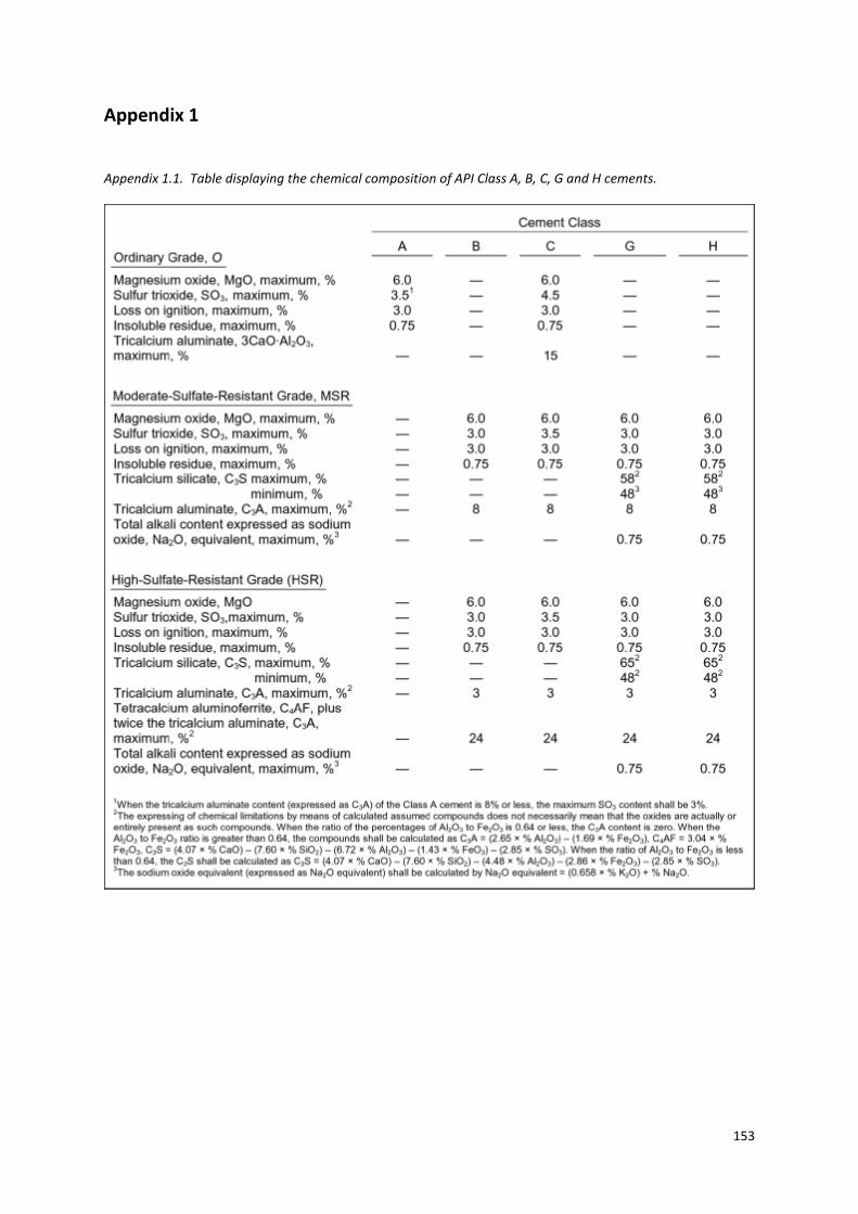
153
Appendix 1
Appendix 1.1. Table displaying the chemical composition of API Class A, B, C, G and H cements.
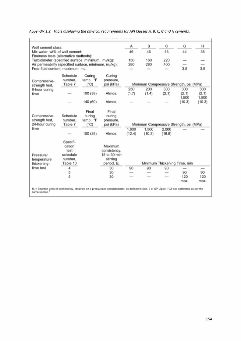
154
Appendix 1.2. Table displaying the physical requirements for API Classes A, B, C, G and H cements.

155
Appendix 1.3. Table displaying the some of the physical properties of API Classes A, C, G and H cements.

156
Appendix 2

157
Table displaying the composition of the hydraulic fracturing fluid used by Cuadrilla at the Preese Hall site.