technical appendix for media, aggregators and the link economy
TRANSCRIPT
Technical Appendix for
�Media, Aggregators and the Link Economy:
Strategic Hyperlink Formation in Content Networks�
Chrysanthos Dellarocas
Zsolt Katona
William Rand
April 24, 2013
1 The anchor selection process
In Section 3 of the paper, we use a reduced form model to account for how consumers select their
anchor node. In this section, we provide a formal micro-model of a process that provides justi�cation
for our assumptions. We also consider the possibility that some consumers may switch their anchor
nodes when encountering a link to a higher quality site and show that including this feature in our
model does not qualitatively change our results.
In common with other analyses of web-browsing behavior, we employ a Markovian model to ab-
stract the anchor node selection process. Model states i = 0, 1, .., N designate which site a consumer
uses as her anchor node. State 0 corresponds to the situation where the consumer anchors herself
at the outside option. We de�ne transition probabilities from one state to another, representing the
likelihood that consumers change their anchor node. We follow the behavior of one randomly selected
consumer and measure the probabilities that the consumer anchors herself at a particular node. Let
pi de�ne the probability that the consumer is anchored at site i = 0, 1, ..N ; p0 corresponds to the
outside option. Let wij measure the transition probability from node i to j, that is, the probability
that the consumer switches her anchor from i to j, given that her current anchor is j. We assume
N∑j=0
wij = 1
for any 0 ≤ i ≤ N. Our goal is to solve for the probabilities p∗i that keep the system in equilibrium.
Formally, we require these probabilities to satisfy
N∑i=0
p∗i = 1 and p∗j =N∑i=0
p∗iwij (11)
for any 0 ≤ j ≤ N, making (p∗0, p∗1, ..., p
∗N ) an eigenvector of the W matrix formed by the wij
1

transition probabilities.
First we model a setup without links and assume that consumers generally stick to their anchor
nodes, but they give them up with some probability and move to the outside option. We assume
that, once a consumer anchors herself at a site, the probability wi0 that she abandons it is inversely
proportional to the content the consumer gets, that is, wi0 = ν/zi, for 1 ≤ i ≤ N, where ν is a
su�ciently small constant.1 When consumers are in the outside option state (state 0), they enter
the market again and choose among one of the sites i = 1, .., N with equal probabilities. The
probability that they choose any given site is inversely proportional to the attractiveness of the
outside option, yielding w0i = ν/µ, for 1 ≤ i ≤ N. Observe that we assume that consumers do not
directly switch from one anchor to another. Switching requires passing through the outside option,
that is, wij = 0 for any 1 ≤ i, j ≤ N pair. The above process captures the notion that consumers
experiment with di�erent anchor nodes and stick to these sites depending on the content they obtain.
If the content is not high, they are more likely to leave and go back to the outside option from where
they start experimenting again, especially if the outside option is not very attractive. Alternatively,
a transition to the outside option can be interpreted as consumer exit, whereas a transition from the
outside option as a new consumer entry.2
The equilibrium condition (11) translates to
p∗i =
(1− ν
zi
)p∗i + p∗0
ν
µ
for any 1 ≤ i ≤ N , leading to p∗i /p∗0 = zi/µ. Thus,
p∗i =zi
µ+ z1 + z2 + ...+ zN, and p∗o=
µ
µ+ z1 + z2 + ...+ zN
which are the anchor tra�c formulae we have assumed in Section 3 of the paper.
Now let us consider a case with links, in particular, the most representative case where all but one
site are linking to one target, node 1. When a consumer encounters a link source, she will eventually
access the link target's content even if she anchors at the link source. In the paper we assume that
the presence of a link does not a�ect the choice of anchor node, because the consumer gets the same
satisfaction even if she has to click to get to the content. Here, we relax this assumption and let
consumers change their anchor node upon observing a link to another node. We assume that, when
a consumer chooses her anchor node (transitioning from the outside option) and observes a link to
another node, she changes her anchor node to the link target with probability α.With this additional
assumption in place, the transition probabilites change from w0i =νµ to w′0i = (1−α) νµ for 2 ≤ i ≤ N
and w′01 = (1+ (N − 1)α) νµ . The rest of the transition probabilites are unchanged. Using these new
transition probabilities, we can calculate the equilibrium anchor selection probabilities, yielding
1In particular, we assume that ν < min(µ/N, z1, z2, ..., zN )2The assumption that consumers transition between anchor nodes only throught the outside option is not critical:
the results would be very similar if consumers immediately moved to other anchor nodes when not satis�ed with one.We decided to use this set of assumptions because it allows us to obtain the exact same functional form of anchortra�c we use in the paper.
2

p∗1 =z1(1 + (N − 1)α)
µ+ z1 + z2 + ...+ zN, p∗i =
zi(1− α)µ+ z1 + z2 + ...+ zN
, and p∗o=µ
µ+ z1 + z2 + ...+ zN
for any 2 ≤ i ≤ N . For two nodes, where site 2 links to site 1 this results in
p∗1 =c1(1 + α)
µ+ 2c1, p∗2 =
c1(1− α)µ+ 2c1
.
The following result shows that, if we rewrite our basic model using the above probabilities, we get
our original results with the simple substitution ρ′ = (1− α)ρ.
Proposition 9. Using the functions L(ρ), NL(ρ) ∈ [0, 2] de�ned in Proposition 1 of the paper, we
obtain that:
1. If µ ≤ NL(ρ(1− α)) then sites do not establish links in equilibrium and c∗i = c∗j = cNL.
2. If µ ≥ L(ρ(1 − α)) then there are two asymmetric equilibria where one site links to the other
and
cT =1− µ2− ρ(1− α)
4+
√(2− ρ(1− α))(4µ+ 2− ρ(1− α))
4>
cS =(1− α)ρcT2cT + µ
3. There is no equilibrium in pure strategies otherwise.
Proof. From equation (3) of Section 3, substituting T = 1, S = 2 we obtain:
tAT = p∗1 =cT (1 + α)
µ+ 2cT, tAS = p∗2 =
cT (1− α)µ+ 2cT
.
The corresponding payo� functions of the link source and target nodes (see Section 4.1) then take
the form:
πS =cT (1− α)µ+ 2cT
ρcS −kS2c2S πT =
cT (1 + α) + (1− ρ)cT (1− α)2cT + µ
cT −kT2c2T (12)
which is equivalent to
πS =cT
µ+ 2cTρ(1− α)cS −
kS2c2S πT =
cT + (1− ρ(1− α))cT2cT + µ
cT −kT2c2T (13)
Comparing (13) with equation (5) of Section 4.1 we see that the two are equivalent with the
simple substitution ρ′ = (1− α)ρ. Therefore, all results that rely on equation (5) also apply to this
setting.
The above result shows that a higher probability α of changing one's anchor node to the link
target is mathematically equivalent to a lower ρ, that is, it reduces the source node's ability to
3

monetize the link target's content. From this result it follows that all results of this paper remain
qualitatively unchanged if we assume that users can change anchor nodes to the link target of their
current anchor node. With reference to Figure 2, for a given ρ, linking becomes less likely as α
increases, because then the e�ective ρ′ = ρ(1 − α) declines. For α = 1 (ρ′ = 0), we either have a
unique no-link equilibrium (low µ) or both the linking and non-linking equlibria coexist (high µ).
2 Endogenous ρ
Throughout the paper, we assume that the proportion of anchor tra�c a link source is able to keep
is �xed and does not depend on the relative content levels. Here, we relax this assumption and allow
ρ to depend on the link target's content. In this way, we can capture the possibility that visitors are
more likely to click on a link when the link target's content is higher. We analyze the case with two
nodes. To ensure analytical tractability, we assume a simple linear dependence. In particular, when
site 1 links to site 2 we assume that the probability that a user arriving to site 1 does not click is
ρ(τ) = max(ρ0(1− τcT ), 0),
where τ measures how strongly the probability of clicking is a�ected by the link target's content.
Naturally, we assume that a higher content attracts more clicks, which is why the probability that
consumers stay at the link source is a decreasing function of the link target's content. Note that
the linear formulation would result in negative probabilities if τ or cT are high, thus we assume that
consumers always click in these cases. However, we will only derive results for parameter values with
an interior solution, therefore we assume τ < 1/2. This formulation allows direct comparison with
our original setup, since τ = 0 is equivalent to our basic model with a �xed ρ = ρ0.
With the exception of the probability of clicking, our setup is equivalent to our basic model,
hence the content levels are the same when sites do not link to each other:
c∗1 = c∗2 = cNL =3− 4µ+
√9 + 8µ
8
Similarly to our main results, we can show that a linking equilibrium is possible.
Proposition 10. There exist thresholds L(ρ0, τ), NL(ρ0, τ) ∈ [0, 2] such that:
1. If µ ≤ NL(ρ0, τ) then sites do not establish links in equilibrium and c∗i = c∗j = cNL.
2. If µ ≥ L(ρ0, τ) > 0 then there are two asymmetric equilibria where one site links to the other
and
cT =4− 2ρ0 + (3ρ0τ − 4)µ+
√(4− 2ρ0 − ρ0τµ)(4− 2ρ0 + (8− 9ρ0τ)µ)
8(1− τ)>
cS =ρ0(1− τcT )cT
2cT + µ
4

3. There is no equilibrium in pure strategies otherwise.
Proof. As in the basic model, we examine when the linking and no-linking equilibria are feasible.
Since we already calculated the possible content levels in the no-linking case, let us consider the
linking equilibrium. When site i links to site j, site j's payo� is
πj←i =2 + ρ0(τcj − 1)
2cj + µc2j −
1
2c2j .
Di�erentiating πj←i with respect to cj yields that site j will invest cT in content if site i links to
it (as given in the proposition). Then, di�erentiating
πi→j =cjρ0(1− τcj)cj + cj + µ
ci −1
2c2i
with respect to ci yields that site i will invest
bi→j(cj) =ρ0(1− τcj)cj
2cj + µ
in content if it links to j, yielding the stated ci = cS if we plug cj = cT .
As in the basic case, to check whether sites have any incentive to deviate from the potential
equilibria, we examine whether the no linking best response would yield higher pro�ts in the linking
case and whether the linking best response would yield higher pro�ts in the no-link case. In the �rst
case, the linking equilibrium holds i�
πi(bi(cT ), cT ) ≤ πS := πi→j(cS , cT ).
Let L(ρ0, τ) denote the value of µ where the above holds with equality. The above inequality holds
for high values of µ, yielding that the linking equilibria exists i� µ ≥ L(δ, ρ). For µ = 0, one can check
that Similarly, let NL(ρ0, τ) denote the value of µ for which πi(cNL, cNL) = πi→j(bi→j(cNL)S , cNL).
Sites do not have an incentive to deviate from the no-link equilibrium i� µ ≤ NL(δ, ρ), completing
the proof.
The results are not substantially di�erent from our basic model. The equilibrium regions are
similar to the case when ρ does not depend on the content levels. Furthermore, the linking equilibrium
is not feasible when µ= 0. Figure 2 shows how the equilibrium regions change as τ increases. As ρ
depends more on the target's content, initially both the linking and non-linking equilibrium regions
expand.
Both types of equilibria are more sustainable because of the following intuition. The clicking
probability's dependence on the target's content creates more incentive for the target to invest in
content. Therefore, in the linking equilibria it is less likely that the source �nds it pro�table to deviate
by giving up the link and directly competing with the target. However, the no-linking equilibrium
is also more sustainable, because both sites have lower incentives to deviate from a symmetric no-
5

a) τ = 0.1 b) τ = 0.2
c) τ = 0.3 d) τ = 0.4
Figure 8: Equilibrium regions as a function of ρ0 and τ . The gray regions depict the parameter
regions where the di�erent equilibria are feasible in the basic model, that is, when τ = 0. The redand green plots show how L(ρ0, τ) and , NL(ρ0, τ) change respectively as τ increases.
6
linking equilibrium by linking to the other one since lowering the content has a more pronounced
negative e�ect by driving away visitors.
Corollary 2. Both the target's content and pro�t are increasing in τ. The source's pro�t and content
are decreasing in τ when ρ0 is small.
Not surprisingly, if the target's content has a positive e�ect on the click-through probability of
the source's visitors the target is better o�. Also, due to the increased incentives, it will invest more
in its content. The source's content and pro�t are decreasing if ρ0 is low, that is, when not many
visitors stay at the source's site. However, when ρ0 is su�ciently high this can change. The target's
increased content level makes the source invest more in its own content to take advantage of the
higher amount of tra�c attracted. Since a high proportion of this tra�c stays at the source this
e�ect outweighs the direct e�ect of losing visitors to the higher content target.
3 Sequential moves
Throughout the paper we assume that sites make their decisions simultaneously. In this Section we
analyze a sequential-move version of the basic two-player model. Site 1, the leader, �rst decides its
content level and whether to link to site 2, the follower.3 The follower then decides its content level
and whether to link to the leader. Let us �rst analyze the case without links, where sites can only
make content investments, but cannot establish links. We use backward induction and consider the
follower's decision. As in the basic model site 2's payo� function is given by
π2 =c2
c1 + c2 + µc2 −
c222
where we set δ = k1 = k2 = 1. Di�erentiating π2 with respect to c2 and setting it to 0 yields that
the best response for site 2:
b2(c1) =1− 2µ− 2c1 +
√1 + 4µ+ 4c1
2.
Plugging this into the leader's payo� function we get
π1 =c212· 3−
√1 + 4µ+ 4c1
1 +√1 + 4µ+ 4c1
.
This function has a unique maximum yielding
c∗1 = cL =
(A3 + 10
3A + 13
)2− 4µ− 1
4,
3Since we assume sequential moves, the follower has not yet produced its content when the leader makes its move.The way to interpret the leader's linking strategy is that site 1 commits to linking to the follower once the latterproduces content (whose quality site 1 can perfectly predict).
7

(a) Content (b) Payo�s
Figure 9: Equilibrium content levels and payo�s when linking is not allowed and players move
sequentially
where
A =
(28 + 54µ+ 6
√81µ2 + 84µ− 6
)1/3
.
which, in turn implies
c∗2 = cF =1− 2µ− 2cL +
√1 + 4µ+ 4cL
2.
Note that we naturally get
cL > cNL > cF and πL > πNL > πF
where cNL is the content level produced by two symmetric sites that cannot link to each other. That
is, the leader has an advantage and can sustain a higher content level, thus making higher pro�ts by
attracting more tra�c. Figure 9 depicts the equilibrium content levels and payo�s as functions of µ.
Moving on to the case with the possibility of links, we can expect that the ability of the leader
to dominate the market without links, makes it more attractive for the follower to deviate from a
non-linking equilibrium and link to the leader. The complete analytical characterization of equilibria
is not possible due to the complexity of the expressions involved, therefore we derive the following
results using numerical analysis.
Proposition 11. There exist thresholds LT (µ), LT (µ) ∈ [0, 1] such that:
1. If ρ < LT (µ) then sites do not establish links in equilibrium and
c∗1 = cL and c∗2 = cF .
8

Figure 10: Equilibrium regions with sequential moves.
2. If LT (µ) < ρ < LT (µ), then the follower links to the target. Furthermore, if L(ρ) ≤ µ, then
c∗1 = cT and c∗2 = cS ,
where L(ρ), cT and cS are the same as in the basic linking equilibrium. If µ < L(ρ), then the
leader produces content above cT to deter the follower from direct competition, forcing it to
link.
3. If LT (µ) < ρ, then the leader links to the follower and
c∗1 = cS and c∗2 = cT ,
As expected, the linking equilibrium is the most likely outcome if players move sequentially.
Figure 10 depicts the parameter regions where the di�erent types of linking equilibria are feasible. For
the most part, the equilibrium is such that the follower links to the target who produces high quality
content. In some cases, the source and target content levels are the same as in the simultaneous-move
case, and the leader can set the optimal content level expecting the follower to link. However, if µ
is below L(ρ) and competition is relatively intense, setting the optimal content level is not enough
9

for the leader. The leader needs to increase its content above the (otherwise) optimal link-target
content level to deter the follower from competing directly in content, forcing it to link. Note that in
this region the linking equilibrium would not be feasible with simultaneously moving players. What
makes linking possible with sequential moves is that the follower can expect the leader to stick to
its original decision and to not revise its content downwards. It is questionable how credible this is
in the online world where links and content levels can change frequently. Although in the majority
of the relevant parameter ranges the equilibrium with a link from the follower to the leader is the
only possible outcome, there are two other types of equilibria. When both ρ and µ are very small,
that is, when the outside option is weak, hence the competition for anchor tra�c is tough and when
most visitors click through links, the unique equilibrium is no linking. The bene�t of linking for the
follower is so low that the leader cannot pro�tably set a high enough content to deter the follower
from competing. On the other extreme, when ρ is close to 1 and the link source is able to keep most
of the tra�c that it attracts using the target's content, the leader will �nd it pro�table to become
the source and link to the follower. The follower in this case has no option but to be a link target
and set the appropriate (relatively high) content level. Note that although the source's content level
is low, it makes higher pro�ts because it pro�ts from most of its visitors.
4 Discrete content choice and mixed strategies
Our basic model with two symmetric nodes results in linking equilibria that are asymmetric with
one site linking to the other. Since there are no symmetric linking equilibria in pure strategies it
is natural to examine mixed strategies. Unfortunately, mixed strategies can be rather complicated
when content decisions are continuous, since in addition to mixing in content decisions, sites can
also decide to link with a certain probability, which results in a joint distribution for content and
linking. To be able to examine mixed strategies, we resort to a simpler version of the model where
content can only be set at two predetermined levels: low and high, denoted by c and c. Since only
the fraction of these content levels is relevant we can normalize c to 1. Furthermore, we can simplify
the cost function since the content decision of a site comes down to the choice between low and
high content levels. Therefore, we can focus on the cost di�erence between these two content levels,
denoted by K. Otherwise, this model is identical to our basic model with two nodes. Both sites
decide their content levels simultaneously and whether to link to each other or not. We �rst analyze
the equilibria in pure strategies. The payo�s in the no linking cases are the following:
πLL =c2
2c+ µ, πHH =
1
2 + µ−K, πLH =
c2
c+ 1 + µ, πHL =
1
c+ 1 + µ−K,
where πLLand πHH denote the payo�s when both sites choose low (high) and πLH and πHL denote
the payo�s when one site choose low and the other high content. Simple analysis of this two-by-two
game shows that there are three possible equilibria in pure strategies.
1. When K > 1c+1+µ −
c2
2c+µ , both sites produce low content levels.
10

2. When 1c+1+µ −
c2
2c+µ > K > 12+µ −
c2
c+1+µ ,one site produces low content and the other produces
high content.
3. Finally, when 12+µ −
c2
c+1+µ > K, both sites produce high content levels.
That is, costs have to be low enough for sites to invest in high content. For direct comparison with
our continuous model, we will focus on the third type of outcome and assume 12+µ −
c2
c+1+µ > K
from this point on while examining linking incentives. Linking is only feasible when the link source
has low content and the link target has high content. The source's and the target's payo�s are the
following:
πS =ρc
2 + µ, πT =
2− ρ2 + µ
.
In order for linking to be an equilibrium we have to make sure that the source does not have an
incentive to deviate to produce high content and sever the link. A deviation is non-pro�table i�
πS > πHH . Examining the no linking equilibrium yields the opposite constraint, resulting in the
proposition.
Proposition 12. Assuming 12+µ −
c2
c+1+µ > K, there are two feasible equilibria
1. If K < 1−ρc2+µ , both sites produce high content levels and do not link to each other
2. If K > 1−ρc2+µ , one site produces low content and links to the other site, which produces high
content.
Note that this result is very similar to our results in the basic model, where linking was not
possible when the cost of content production was low, because sites �nd it pro�table to produce high
content themselves. If the costs are above a certain level, this changes and one site �nds it pro�table
to produce low content and link to its high-content peer. Depending on the values of ρ and µ the
regions where linking is possible can be empty. In fact, linking is possible with a suitable cost if and
only if
ρ ≥ c(2 + µ)
c+ 1 + µ.
Figure 11 shows that the region where linking is possible exhibits similar features as in the basic
model. Just as in the continuous case, linking is only possible when µ is high so that competition
between sites is relatively weak. Furthermore, linking in this case requires that ρ is high enough that
the link source can capture a high percentage of the extra tra�c. Finally, the region where linking
is possible expands as the content di�erence between high and low increases which is consistent with
the previous results.
Now that we have examined the discrete case in detail, let us analyze mixed strategy equilibria.
In particular, we are going to focus on the parameter region, where the pure strategy equilibrium
is asymmetric, that is, where a low quality site links to a high quality site. Thus, we will assume1
2+µ −c2
c+1+µ > K > 1−ρc2+µ from now on. Since linking to a high quality site is always better
than producing low quality without linking, sites must mix between producing high quality content
11

(a) c = 0.25 (b) c = 0.5
Figure 11: Feasibility of linking equilibrium in the discrete content choice case.
without linking and low quality content with linking. The only outcome that we have not encountered
before is if both sites decide to produce low quality content and link to each other, but the payo�s
will be simply πLL. Let us determine the symmetric equilibria in mixed strategies and let pL denote
the probability of setting low quality content while linking to the other site. In equilibrium the mixed
strategy of one site must make the other site indi�erent between the two options, therefore
pLπLL + (1− pL)πS = pSπT + (1− pS)πHH .
This leads to the following result.
Proposition 13. If 12+µ −
c2
c+1+µ > K > 1−ρc2+µ , the unique symmetric equilibrium of the game
consist of setting low quality content and linking to the other site with probability
pL = 2c+µ1−c ·
K(2+µ)+ρc−1(2(1−ρ)+µ)c+µ(1−ρ) ,
and setting high content without linking with probability 1− pL.
The result is rather intuitive. As the cost of producing high quality content increases, it is more
likely that sites will choose to produce low quality content and establish a link. When the cost reaches
a critical level the probability reaches 1, but then linking will be worthless as nobody produces high
quality content and there is no point in linking. The probability of becoming a link a source also
increases in ρ since the link source can capture more of the anchor tra�c.
12

5 Link refusal between two homogeneous sites
Here, we modify the basic homogeneous two player (no aggregator) model and allow link targets
to veto (refuse) a link after it has been created by the link source. In contrast to the simultaneous
linking and content decisions that we examined in the case without link refusal, in this model sites
�rst make their decisions on content investments, and then they decide whether they want to link
to another site. Finally, each link target decides whether it allows or refuses the link.4
As one would expect, a site refuses a link from its peer if the link source's content is low relative
to the link target. Simple calculations show that a link from site i to site j will be accepted by the
target as long as
ci ≥ρcj − µ(1− ρ)
2− ρ.
Otherwise, the link will be refused by the target and sites will rely on their own content. When
sites are heterogeneous, the above argument implies that targets will refuse links from ine�cient
competitors. When the competing sites are homogeneous, the following result summarizes how this
a�ects content and linking decisions and how it changes the results of Proposition 1 of the paper..
Proposition 14. There exist thresholds SCL(ρ) ≥ CL(ρ) ≥ L(ρ) and NCL(ρ) ≥ NL(ρ) such that:
1. If kµ ≤ NCL(ρ) then sites do not establish links in equilibrium and c∗i = c∗j = cNL.
2. If kµ ≥ SCL(δρ) then there are two asymmetric equilibria where one site links to the other
and c∗i = cS ≤ c∗j = cT , which is identical to the case without possible link refusal.
3. If SCL(ρ) ≥ µ ≥ L(ρ) then there are two asymmetric equilibria where one site links to the
other and
c∗i =ρcT − µ(1− ρ)
2− ρ≥ cS , c∗j = cT
4. There is no equilibrium in pure strategies otherwise.
Figure 12 illustrates that the results are similar to the case when links cannot be refused but
the ability to refuse links makes linking less likely. The parameter region in which linking is feasible
shrinks, especially for high values of ρ. This is not surprising, since link targets are hurt the most
when link sources are able to retain a high proportion of the tra�c they attract. The region of the
no-link equilibrium, on the other hand, expands, and the net result is a potential reduction in pro�ts
due to the increased competition without links. Nonetheless, for a wide range of parameters, linking
is still feasible. If µ is high enough this happens because both the target and the source are better o�
when linking due to the reduced competition within the content ecosystem and increased audience
of link equilibria that is diverted from the competitive outside alternative.
We observe an interesting phenomenon in an intermediate region: when µ is not high enough to
provide enough bene�ts to the target under our standard linking equilibrium, the link source will
4Our results do not change if we reverse the order of link creation by the source and the refusal decision by thetarget as long as these decisions are made after the content investments have been settled.
13
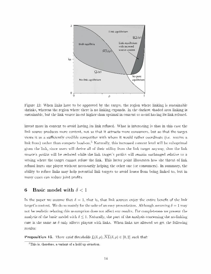
Figure 12: When links have to be approved by the target, the region where linking is sustainable
shrinks, whereas the region where there is no linking expands. In the darkest shaded area linking is
sustainable, but the link source invest higher than optimal in content to avoid having its link refused.
invest more in content to avoid having its link refused. What is interesting is that in this case the
link source produces more content, not so that it attracts more consumers, but so that the target
views it as a su�ciently credible competitor with whom it would rather coordinate (i.e. receive a
link from) rather than compete head-on.5 Naturally, this increased content level will be suboptimal
given the link, since users will derive all of their utility from the link target anyway, thus the link
source's pro�ts will be reduced while the link target's pro�ts will remain unchanged relative to a
setting where the target cannot refuse the link. This latter point illustrates how the threat of link
refusal hurts one player without necessarily helping the other one (or consumers). In summary, the
ability to refuse links may help potential link targets to avoid losses from being linked to, but in
many cases can reduce joint pro�ts.
6 Basic model with δ < 1
In the paper we assume that δ = 1, that is, that link sources enjoy the entire bene�t of the link
target's content. We do so mainly for the sake of an easy presentation. Although assuming δ = 1 may
not be realistic relaxing this assumption does not a�ect our results. For completeness we present the
analysis of the basic model with δ ≤ 1. Naturally, the part of the analysis concerning the no-linking
case is the same as δ only a�ects players with links. When links are allowed we get the following
results:
Proposition 15. There exist thresholds L(δ, ρ), NL(δ, ρ) ∈ [0, 2] such that:
5This is, therefore, a variant of a hold-up situation.
14
1. If kµ ≤ NL(δ, ρ) then sites do not establish links in equilibrium and c∗i = c∗j = cNL.
2. If kµ ≥ L(δ, ρ) then there are two asymmetric equilibria where one site links to the other and
cS =δρ
k(1 + δ)· 1 + δ(1− ρ)− 2kµ+
√(1 + δ(1− ρ))2 + 4(1 + δ(1− ρ))kµ
1 + δ(1− ρ) +√(1 + δ(1− ρ))2 + 4(1 + δ(1− ρ))kµ
≤
≤ cT =1
k(1 + δ)· 1 + δ(1− ρ)− 2kµ+
√(1 + δ(1− ρ))2 + 4(1 + δ(1− ρ))kµ
2.
3. There is no equilibrium in pure strategies otherwise.
Proof. There are two possible types of equilibrium with respect to linking: (i) the one where there
is no link between the two sites and they invest equally in content (cNL), and (ii) the one where one
site invests less in content and links to the other site. As we have already determined the potential
equilibria of the �rst type, we will now identify the candidates for linking equilibria, then check when
neither site has an incentive to deviate from a potential equilibrium. When site i links to site j, then
its pro�t becomes
πi→j =δcjρ
δcj + cj + µci −
ki2c2i .
Comparing these two yields that site i will link to site j i�
ci ≤δρcj(cj + µ)
(1 + δ(1− ρ))cj + µ.
Note that the right hand side of the above equation is increasing in cj and always less than
or equal to cj , yielding that only the lower quality site will establish a link and only if its quality
is su�ciently low relative to its competitor. Given the above described linking behavior, sites will
choose their content investments to maximize pro�ts. Although the site that ends up with a higher
content does not consider linking, its pro�t function changes if its low content competitor decides to
link to it:
πj←i =cj + δ(1− ρ)cjδcj + cj + µ
cj −kj2c2j .
Di�erentiating πj←i with respect to cj yields that site j will invest cT in content if site i links to
it (as given in the proposition). Then, di�erentiating πi→j with respect to ci yields that site i will
invest
bi→j(cj) =δρcj
(cj + cjδ + µ)k
in content if it links to j, yielding the stated ci = cS if we plug cj = cT .
To check whether sites have no incentives to deviate from the potential equilibria, we examine
whether the no linking best response would yield higher pro�ts in the linking case and whether the
linking best response would yield higher pro�ts in the no-link case. In the �rst case, the linking
15

equilibrium holds i�
πi(bi(cT ), cT ) ≤ πS := πi→j(cS , cT ).
Let L(δ, ρ) denote the value of µ where the above holds with equality when k = 1. It is easy
to check that the above inequality is invariant to the values of µ and k as long as µk is �xed.
Furthermore, it holds for high values of µk, yielding that the linking equilibria exists i� µk ≥ L(δ, ρ).Similarly, let NL(δ, ρ) denote the value of µk for which πi(cNL, cNL) = πi→j(bi→j(cNL)S , cNL). Sites
do not have an incentive to deviate from the no-link equilibrium i� µk ≤ NL(δ, ρ), completing the
proof.
7 Multiple sites: high linking costs and more than one link target
In the paper, we analyze the model with N > 2 sites and small KL>0 costs. We conclude that
in most cases there are no links, or if there are, there is a single link target (NT = 1). Here, we
provide details about the cases when KL is not necessarily close to 0 and when NT > 1. We start by
discussing the implications of increasing KLon the equilibria with no links or a single link target then
we analyze the case of multiple link targets. The existence of an equilibrium without links hinges on
the lack of pro�table deviations for sites in which they would become link sources and link to their
peers. Naturally, as the cost of linking increases such a deviation is even less pro�table. Therefore,
the parameter region where an equilibrium without links is possible expands as KL increases. That
is, if a no linking equilibrium exists for a certain (ρ,N) pair for KL,then a no linking equilbrium
has to exist for the same (ρ,N) pair for a higher cost K ′L > KL. Indeed, by analyzing the pro�t in
the no linking equilibrium and the pro�t with a potential deviation (not counting the linking cost),
the increment is at most 1/32, therefore a no linking equilbrium always exists (for any ρ and N) i�
KL ≥ 1/32. While the no linking equilibrium region expands as KLincreases, the opposite is true
for the region where a single link target equilibrium is possible. However, such an equilibrium will
always be possible with a high enough N , even when KL is very high (Figure 7 shows the equilibrium
regions as KLincreases).
Now we move on to examine equilibria with multiple targets. We �rst focus on KL → 0, then
examine the case of higher costs. As stated in the paper, in equilibrium, we must have
cS =ρ
N, cT =
(2NT − 1)(ρNT + (1− ρ)N)
N ·N2T
.
In order to determine the feasibility of such an equilibrium, we have to rule out pro�table deviations.
The condition for pro�table deviations for sites that are link sources are essentially the same when
there is one target or more. However, the condition for a link targets' deviation is fundamentally
di�erent. When there is only one link target, it can never deviate pro�tably, since there is no other
reasonable quality sites to link to. On the other hand, when there is more than one link target, each
link target can consider lowering its content and linking to another link target. The pro�t that a
16

a) KL = 0 b) KL = 0.003
c) KL = 0.01 d) KL = 132
Figure 13: Equilibrium regions as KL increases.
17
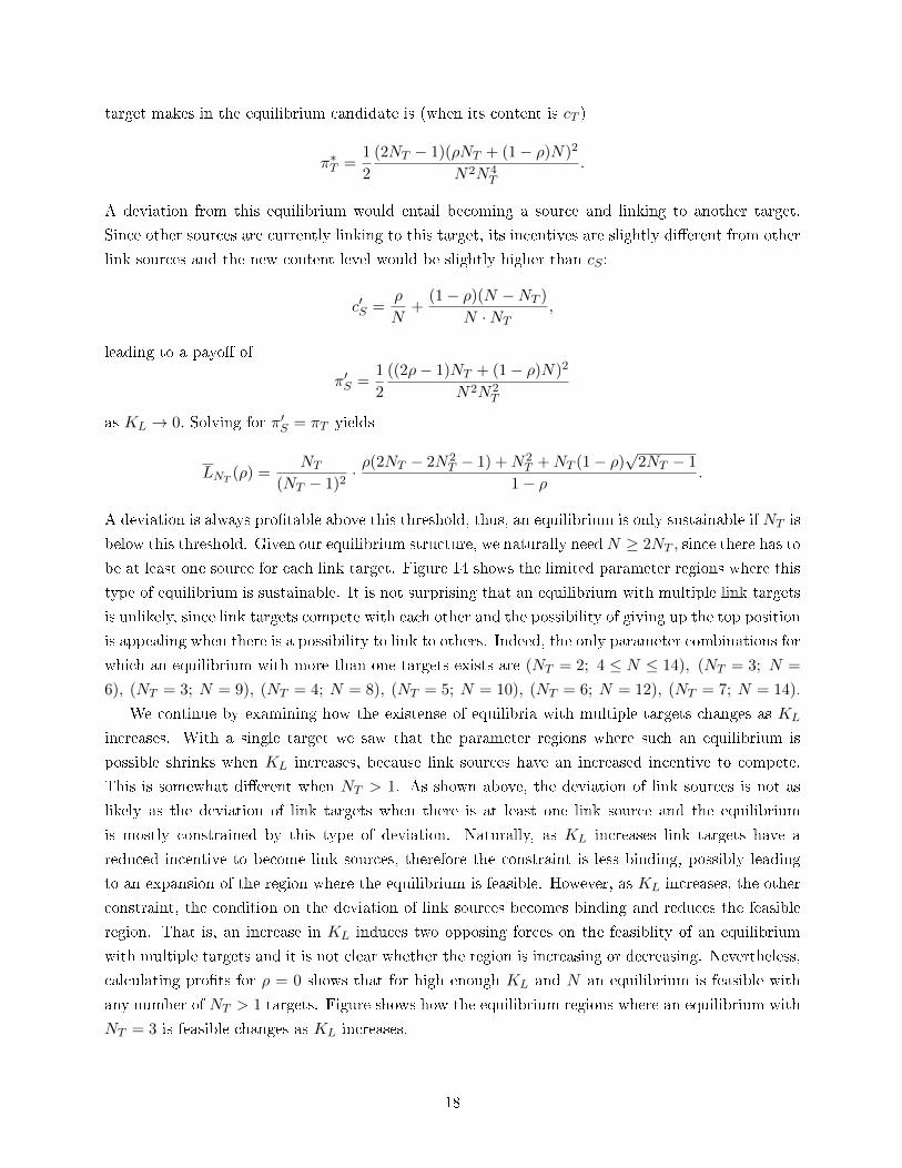
target makes in the equilibrium candidate is (when its content is cT )
π∗T =1
2
(2NT − 1)(ρNT + (1− ρ)N)2
N2N4T
.
A deviation from this equilibrium would entail becoming a source and linking to another target.
Since other sources are currently linking to this target, its incentives are slightly di�erent from other
link sources and the new content level would be slightly higher than cS :
c′S =ρ
N+
(1− ρ)(N −NT )
N ·NT,
leading to a payo� of
π′S =1
2
((2ρ− 1)NT + (1− ρ)N)2
N2N2T
as KL → 0. Solving for π′S = πT yields
LNT(ρ) =
NT
(NT − 1)2· ρ(2NT − 2N2
T − 1) +N2T +NT (1− ρ)
√2NT − 1
1− ρ.
A deviation is always pro�table above this threshold, thus, an equilibrium is only sustainable if NT is
below this threshold. Given our equilibrium structure, we naturally needN ≥ 2NT , since there has to
be at least one source for each link target. Figure 14 shows the limited parameter regions where this
type of equilibrium is sustainable. It is not surprising that an equilibrium with multiple link targets
is unlikely, since link targets compete with each other and the possibility of giving up the top position
is appealing when there is a possibility to link to others. Indeed, the only parameter combinations for
which an equilibrium with more than one targets exists are (NT = 2; 4 ≤ N ≤ 14), (NT = 3; N =
6), (NT = 3; N = 9), (NT = 4; N = 8), (NT = 5; N = 10), (NT = 6; N = 12), (NT = 7; N = 14).
We continue by examining how the existense of equilibria with multiple targets changes as KL
increases. With a single target we saw that the parameter regions where such an equilibrium is
possible shrinks when KL increases, because link sources have an increased incentive to compete.
This is somewhat di�erent when NT > 1. As shown above, the deviation of link sources is not as
likely as the deviation of link targets when there is at least one link source and the equilibrium
is mostly constrained by this type of deviation. Naturally, as KL increases link targets have a
reduced incentive to become link sources, therefore the constraint is less binding, possibly leading
to an expansion of the region where the equilibrium is feasible. However, as KL increases, the other
constraint, the condition on the deviation of link sources becomes binding and reduces the feasible
region. That is, an increase in KL induces two opposing forces on the feasiblity of an equilibrium
with multiple targets and it is not clear whether the region is increasing or decreasing. Nevertheless,
calculating pro�ts for ρ = 0 shows that for high enough KL and N an equilibrium is feasible with
any number of NT > 1 targets. Figure shows how the equilibrium regions where an equilibrium with
NT = 3 is feasible changes as KL increases.
18

Figure 14: Feasible parameter regions for an equilibrium with NT > 1 link targets.
19
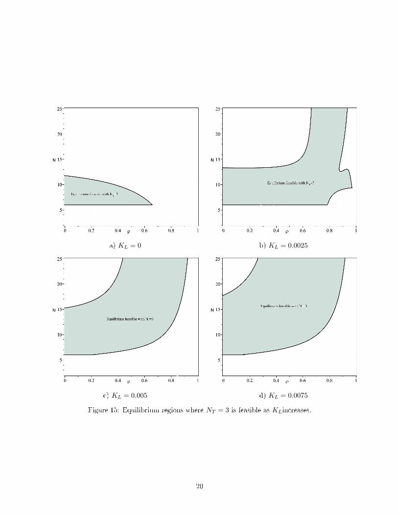
a) KL = 0 b) KL = 0.0025
c) KL = 0.005 d) KL = 0.0075
Figure 15: Equilibrium regions where NT = 3 is feasible as KLincreases.
20