Technical Analysis, Liquidity Provision,and Return Predictability

April 29, 2011

Abstract

We develop a strategic trading model to study the liquidity provision role of tech-

nical analysis. The equilibrium prices are semi-strong efficient, returns are negatively

correlated. Technical traders use past prices to forecast the liquidity premium, which

is not related to the fundamental information, and thus provide implicit liquidity to

the market in additional to risk-averse liquidity providers. Interestingly, informed

traders and technical traders have similar trading patterns: They employ contrarian

strategies, their orders have positive price impacts, and forecast short-horizon futures

returns. If we interpret the technical traders as individual traders, then our model

explain the documented puzzling empirical results regarding individual investors,

who are contrarians and whose order are positively related to future returns in the

short term. We also show technical trading reduces price predictability and enhances

market efficiency by improving the price discovery process, increasing price informa-

tiveness, and reducing price impact and price volatility.

Keywords: Technical Analysis, Liquidity Provision, Inventory Effect, Contrarian

Strategy, Return Predictability

JEL classification: G11, G12, G14

1

1 Introduction

Technical analysis is a security analysis discipline to forecast the direction of future pricesusing primarily past prices and volumes information. Academics do not reach consen-sus whether technical analysis is useful to investors.1 However, technical analysis is verypopular in the investment industry and considered very useful. Many investment reportsand advisory services of brokerage firms are based on technical analysis. Many hedgefunds, investment bank, and proprietary trading desks employ some technical tradingstrategies. Given price and volume data are easily and cheaply available, technical analy-sis is also very popular among individual investors, who are usually limited by resourcesand capabilities to conduct fundamental research.

Though technical analysis plays an important role in investment, theoretical analysisof it has been limited. Previous theoretical models usually focus on the role of technicalanalysis to figure out the information of fundamental value. Instead, this paper takes adifferent angle and develops a Kyle-type equilibrium model to explore the relationshipbetween technical analysis and liquidity provision.2 More specifically, we address thefollowing questions: What is the relationship between technical trading and liquidityprovision in the short term? What is the effects of technical trading on price discoveryprocess and market quality, such as price informativeness, price variability, price impact.What is its effect on return predictability? What is the trading pattern of technical traderswho have no private information? These questions are not widely addressed in existingtheoretical studies.3

We consider a three-period model. The stock payoff is realized at date 3. Tradinggame takes place at date 1 and date 2. There are four types of traders: a risk-neutralinformed trader, noise traders who trade for exogenous motives, a risk-neutral technical

1See detailed discussion in the literature review.2A less contentious empirical finding shows that there exists a positive relationship between technical

analysis and liqudity provision. More specifically, Kavajecz and Odders-White (2004) demonstrate thatsome technical trading rules such as support and resistance levels coincide with peaks in depth on the limitorder book and moving average forecasts reveal information about the relative position of depth on thebook.

3As the subsequent literature review shows, they mainly focus on the information extraction role oftechnical analysis, but its implications on trading, asset pricing and welfare have not been sufficiently ex-amined. Limited in number, most of these studies are developed in the competitive rational expectationparadigm and rules out the strategic interplay among investors, which we believe is an important featureof technical analysis. One exception is Brunnermeier (2005) who shows that technical analysis can playa role in the strategic rational expectation models under the SEC’s Regulation Fair Disclosure. The early-informed traders will employ technical analysis after the public announcement to determine the extent towhich the news is already impounded into price. Consequently, their trading behavior is consistent withthe street wisdom “buy on (positive) rumors and sell on news”.

2

trader who trade based on historical prices and volumes, and risk-averse (CARA) liq-uidity providers, who know the equilibrium price and maximize their expected utilityat date 3 and their order clear markets. The prices are functions of available order flowand public information. After two-period trading the game ends and all traders receivepayments according to the stock payoff and their security holdings. The informed traderknows the stock payoff and the rest only knows its distribution. The informed trader, thetechnical trader, as well as noise traders submit market orders to competitive risk averseliquidity providers. The informed trader and the technical trader both trade strategicallyby taking into the impacts of their trades on equilibrium prices. It is worth noting thatrisk aversion is a tractable way to model the constraints faced by liquidity providers sothat they cannot provide costless immediacy services. For example, it may capture riskneutral immediacy subject to funding or VaR constraints.4 Hence, the liquidity providersare "effective risk averse".

We show that the price comprises two components because of risk aversion, the fairvalue, which is the fundamental value conditional on liquidity providers’ informationset, and the liquidity premium to compensate the liquidity providers for holding unde-sired risky positions. Risk aversion causes the equilibrium price to deviate from the fairvalue. Since this deviation is not driven by information regarding the fundamental value,a correction is expected in the next period. Hence, returns are negatively autocorrelated.In comparison, when liquidity providers are risk-neutral (face no constraints), the liquid-ity providers earn zero expected profits because of competition; the price is equal to thefair value, and prices follow a martingale process.5 The returns are thus independent ofeach others. Because technical trader provider extra liquidity to the market, the liquiditypremium demanded by the liquidity provider is partially reduced, the magnitude of thenegative return autocorrelations decline. Hence, the existence of technical trader reducesprice predictability and enhances market efficiency.

In our model, the technical trader trades as a contrarian, and his trade positively fore-casts future returns. Intuitively, the technical trader knows that by providing extra liquid-ity to the market, he can earn part of the liquidity premium demanded by the liquidityproviders. He thus chooses to trade in the opposite direction of previous price change inperiod 1. Because he and the informed trader trade taking into account the price impact,

4See, e.g., Danielson, Shin, Zigrand (2010) and Adrian, Etula, Shin (2010).5The risk averse liquidity providers are prevalent in the competitive rational expectation paradigm pi-

oneered by Grossman and Stiglitz (1980) and Hellwig (1980) but are relatively rare in the strategic rationalexpectation model initiated by Kyle (1985). Subrahmanyam (1991) first introduces risk averse market mak-ers into Kyle (1985). The effect of liquidity providers’ risk aversion on return dynamics such as momentum,reversal and post-earning announcement drifts is studied in Guo and Kyle (2010).

3

the price reverses to the fair value only partially. Hence, his position is positively corre-lated with the next period return in period 3. Because individual investors on averageare less informative in comparison with institutional investors, they are more likely toadopt technical analysis to trade. If we interpret the technical trader in our model as Indi-vidual investors, these predictions are consistent with numerous empirical findings thatindividuals tend to be negative feedback traders or contrarians.6 Our results also explainwhy the net flows of small investors positively predict future short-horizon returns asdocumented by Jackson (2003), Kaniel, Saar, and Titman (2008) , and Barber, Odean andZhu (2009), among others. Since the individual investors lack information advantage, it isusually hard to understand why the trade of individual investors has short term forecast-ing ability. Our model shows that the forecasting power may come from implicit liquidityprovision instead of information advantage. Our model further shows that technical trad-ing is more profitable when the fundamental risk is larger, when the noise trader risk islarger, and (or) when the liquidity providers become more risk averse. Intuitively, anincrease in the fundamental risk, noise trader risk, and (or) risk aversion coefficient willcause the prices to be more predictable (measured by return autocorrelation). Kaniel et al.(2008) finds that individual investors’ order has more forecasting power for small stock.Small stocks usually involve larger fundamental risk and less liquidity. Hence, all theabove results shows that the observed trading patterns of the technical traders is consis-tent with our story of liquidity provision. It is worth noting that our model shows thatliquidity provision can be due to market orders. Remarkably, the technical trader and theinformed trader in our model display similar trading patterns: they employ contrariantrading strategy in the second period, their trades have positive price impact on the price,and their trades positively forecasts futures returns. However, as discussed before, theytrade for different purposes: the informed trader trades because of his informational ad-vantage whereas the technical trader trades for the purpose of liquidity provision. Theimplications for empirical studies is that it is not enough to study only the lead-lag or con-temporaneous relationships between trades and return to determine whether the trade isinformational.

Furthermore, our model also shows that technical trading enhances price discoveryprocess. Compared with the case of no technical trading, price becomes more informative,price volatility declines, and price impacts reduce. Our model demonstrates technicaltrading in the short run mainly provide implicit liquidity to the markets.

The remainder of the paper is organized as follows. Section 2 reviews several strands

6See, Choe, Kho, and Stulz (1999) , Grinblatt and Keloharju (2000, 2001) , Jackson (2003), Richards (2005),Goetzmann and Massa (2002) , and Griffin, Harris, and Topaloglu (2003), among others.

4

of relevant literature on technical analysis and liquidity provision. Section 3 developsa three-period strategic trading model in which an informed trader and an uninformedtraders employing technical analysis trade against risk averse liquidity providers. Forthe purpose of comparison, we also derive the equilibrium in the absence of uninformedtraders. Section 4 studies the impact of technical analysis on trading strategies, liquidityprovision, asset pricing patterns, and welfare implications. Section 5 studies several ex-tensions of the benchmark model. Section 6 concludes. All the proofs are delegated to theAppendix.

2 Literature Review

Technical analysis of price and volume patterns has long been regarded as pointless whenthe efficient market hypothesis is deemed indisputable in the finance research. In fact, thisview is strengthened by early study such as Fama and Blume (1960) who show that com-mon filter rules could not outperform the simple buy-and-hold strategy after transactioncosts. Economists’ enthusiasm in searching for profitable technical analysis is re-ignitedwhen amounted evidence against market efficiency has emerged since 1980s. Influen-tial studies by Brock, Lakonishok, and LeBaron (1992), Lo, Mamaysky, and Wang (2000),LeBron (1999), and Neely (2002), among others, find positive value of some widely em-ployed technical trading rules in stock and foreign exchange markets. However, thesestudies attract followers as well as critics. Economic and statistical issues such as riskadjustment, data-snooping bias, survivorship bias have been raised and examined (Sul-livan,Timmermann, and White,1999; Allen and Karjalainen, 1999), but the controversyseems far away from being settled. According to Park and Irwin (2007), among a total of95 modern studies, 56 studies find positive results regarding technical trading strategies,20 studies obtain negative results, and 19 studies indicate mixed results.

The far-reaching popularity and wide employment of technical analysis among prac-titioners does not receive its theoretical justification until Treynor and Furguson (1985)who defend that past price patterns help a trader to determine whether her informationis unique to herself or is common to everyone. In the competitive rational expectationmodels, Grundy and McNichols (1989), and Brown and Jennings (1989) show that techni-cal analysis of prices has positive value to traders because a single price does not revealthe risky asset’s fundamental information but a sequence of prices does under certain con-ditions. By introducing higher-order uncertainty on quality of asymmetric information,Blume, Easley and O’Hara (1994) show that in addition to learning from price patterns,

5

technical analysis of volumes can improve trader’s learning of fundamentals. Traderswho use information contained in both will do better than traders who do not. Thesetheoretical rationales for technical analysis are nicely reviewed by Brunnermeier (2001).Nonetheless, these theoretical support does not mean that specific techniques based onrecognizing “head-and-shoulers” patterns or “support and resistance levels” and “mov-ing average” can be grounded on the extant models. Zhu and Zhou (2009) attempt to fillthe gap by studying the use of moving average, the arguably most popular trading rules,in a standard asset allocation problem. They provide conditions such that fixed alloca-tion rules in conjunction with technical analysis can outperform parameter-dependentoptimal learning rule. However, Zhu and Zhou (2009) depart from the prior work ontechnical analysis in that the asset return process is exogenously given rather than en-dogenously generated in their model.

We next review the liquidity provision role of market makers and individual traders.Kaniel, Saar and Titman (2008) suggest that their findings that uninformed individualinvestors employ contrarian and their trade positively forecast the future returns are con-sistent with the theoretical predications proposed by Grossman and Miller (1988), andCampbell, Grossman, and Wang (1993), that risk-averse individuals act as contrarians toprovide liquidity to meet institutional demand for immediacy, and the price concessionsprovided by the latter naturally lead to subsequent return reversals. The same idea isshared by Hendershott, Li, Menkveld, and Seasholes (2010).

While we largely agree with this wisdom, a number of questions arise in our mind.First, we wonder what drives the individuals to replace the role of market makers whoare assigned to take the liquidity provision job. Actually in Grossman and Miller (1998),it is market makers that provide liquidity to immediacy needed individuals and chargefor bearing price risk, “although in practice, of course, individuals and firms can playeither role at different times.” (p.622). If individuals are equally being the demanders andsuppliers of immediacy, their trades should not exhibit clear styles and should not be ableto forecast future returns. Second, we wonder if the explanation is robust if the lack ofimmediacy as a result of trading asynchronization is less of a concern in today’s marketsthat are characterized by high trading volume and market liquidity. Last but not the least,we wonder if the risk aversion of individual investors is a pre-condition for the results tohold in the existing theories.

To address these concerns in our strategic trading model we purposefully introducethe market makers, who could be any non-individual entity that provides liquidity, to re-lieve such responsibility from individual investors. Hendershott et al. (2010) also departfrom existing models and demonstrate the liquidity provision role of market makers di-

6

rectly but their objective is different from ours. Moreover, the informed and uninformedinvestors in their model are risk averse. We consider the market order so that the effectof trading asynchronization is minimized. In general, this type of order will be executedimmediately and investors do not have to worry about the delay.

Despite the difference, our analysis is complementary to Grossman and Miller (1988),Campbell, Grossman, and Wang (1993), Hendershott et al. (2010). In particular, we showthat the risk aversion of uninformed investors is not a necessary condition for the liquidityprovision argument to hold.

Last but not the least, our model can be placed in the literature initiated by Admati andPfleiderer (1988) which studies the strategic trading of uninformed traders in choosingeither the composition or the timing of their trades. We contribute to this literature byshowing the rich trading and asset pricing patterns when the informed, uninformed tradestrategically against a risk averse liquidity providers.

3 The Model

We develop a three-period trading model in the strategic rational expectation paradigmpioneered by Kyle (1985). In this benchmark economy one risk-free bond and one riskystock are available for trading. We assume that the interest rate for the bond is zero andthat the price of the bond is always one for convenience. The stock payoff D is normallydistributed with mean D and variance σ2

D. Before trading starts the price of the stock isgiven by P0 = D. The stock payoff is realized at date 3. Trading game takes place atdate 1 and date 2 with four types of traders: a risk-neutral informed trader, noise traderswho trade for exogenous motives, a risk-neutral technical trader who trades based onhistorical prices patterns, and a continuum of risk-averse competitive liquidity providerswho observe the total order flows, choose trade and price to maximize expected profitsand clear the market. After two-period trading the game ends and all traders receivepayments according to the stock payoff and their security holdings. The informed traderknows the true value of stock payoff and the rest only knows its distribution. We stressthat the model is a short term model because no additional information arrives in themarket. The assumption on no dynamic information is used to capture the trading andasset pricing patterns in short horizon.

As in Kyle (1985), trading in each period t ∈ {1, 2} occurs in two steps. In the firststep, the informed trader, the technical trader, and noise traders submit their market or-ders. In the second step, the liquidity provider observes the net order flows, sets the

7

prices and clears the market. Except for the noise traders, other traders choose tradingstrategies to maximize their expected profits respectively. The informed trader initiatestrading and chooses his optimal trading strategies Xt at date t. The technical trader doesnot trade at date 1 but picks his optimal trading quantity Z at date 2 conditional on thehistorical prices information P0 and P1. The noise traders submit their total orders Ut atdate t where Ut are normally distributed with mean zero and variance σ2

U. In addition,U1 and U2 are independent from each other and from the stock payoff D. Without lossof generality the total mass of liquidity providers is normalized to unity. We depart fromKyle (1985) by assuming that the representative liquidity provider has a CARA utilityfunction − exp (−γWY

3 ), where γ denotes the risk-aversion coefficient, and WY3 denotes

the liquidity provider’s accumulated wealth at date 3. After observing the the total orderflows ωt in period t submitted by other traders, where

ω1 = X1 +U1

ω2 = X2 + Z+U2

the representative liquidity provider chooses her optimal positions Yt and sets the com-petitive prices Pt not only to maximize her expected utility but also to clear the market.The initial endowments of all traders are normalized to be zero to simplify the analysiswithout affecting any propositions. As will be evident in the subsequent analysis, the riskaversion assumption of the liquidity provider is essential for our main results while therisk neutrality assumption of the informed and technical traders are just for convenience.

Next, we specify the equilibrium stock price, the market clearing condition and theequilibrium trading strategies by the liquidity provider, the informed trader and the tech-nical trader respectively in each period. Following the convention we restrict our atten-tion to a linear equilibrium, which is decomposed into three parts. First, in each periodthe stock price is a linear function of liquidity providers’ state variables. She sets equilib-rium price from the conjectured trading strategies of the informed and technical tradersand her updated beliefs about the stock payoff. She maximizes her expected utility bychoosing her position in stock which clears the market. Second, given the pricing rule,the liquidity provider’ updated beliefs, and the technical trader’s trading strategy in eachperiod, the informed investor figures out his investment opportunities and chooses hisoptimal trading strategy. His order flow is a linear function of his state variables. Third,given the pricing rule, the liquidity provider’s updated beliefs, and the informed trader’strading strategy in each period, the technical trader chooses his optimal trading strategy,which is a linear function of past prices.

8

To solve the linear equilibrium, we begin by postulating that the equilibrium stockprices in each period are given by

P1 = λ10 + λ11ω1, (3.1)

P2 = λ20 + λ21ω1 + λ22ω2. (3.2)

The coefficients λ′s are constants to be determined in the equilibrium and λ11, λ21 and λ22

are liquidity parameters. Because the liquidity provider sets prices based on her observedorder flows of other traders, two implications follow naturally. First, Pt depends on theorder flows up to period t therefore price in period 2 is a function of ω1 and ω2. Sec-ond, the liquidity provider’s optimal holdings Yt in the stock do not appear in the pricefunctions.

To clear the market clears, the sum of the positions of the informed trader, the technicaltrader, noise traders, and the liquidity provider must be equal to zero in each period:

X1 +U1 +Y1 = 0, (3.3)

X2 + Z+U2 +Y2 = 0. (3.4)

Using the pricing functions and the market clearing conditions, we are able to rigorouslysolve the dynamic maximization problems of the informed trader, the technical trader,and the liquidity provider to determine their optimal trading strategies as well as thecoefficients in the pricing functions.

We conjecture that the linear trading strategies of the informed trader in each periodare given by

X1 = β10 + β11D, (3.5)

X2 = β20 + β21D+ β22ω1 + β23Z. (3.6)

The coefficients β′s are constants to be determined in the equilibrium and β11, β21 andβ22 measure informed trader’s trading intensity. It is worth noting that the informedtrader trades only on private information in period 1, but in period 2 he trades on privateinformation as well as date-2 public information ω1, which is informationally equiva-lent to price P1. More importantly, because the technical trader’s order Z depends onP0 and P1 which are publicly observable, the informed trader could infer this quantityin equilibrium and will therefore take into account its impact on the equilibrium price.Consequently, the informed trader’s trading strategy in period 2 also depend on Z.

Since observing P1 is equivalent to observing ω1, we conjecture that the linear trading

9

strategy of the technical trader in period 2 is given by

Z = h0 + h1ω1. (3.7)

The coefficients h′s are constants to be determined in the equilibrium and h1 measurestechnical trader’s trading intensity.7 The uninformed technical trader does not trade inperiod 1 to avoid losing money to the informed.

Taking above analysis together, we see that while the technical trader is a pure techni-cian, the informed trader is a partial fundamentalist and a partial technician. Both exploitthe historical prices and order flows patterns, which are informationally equivalence inthe benchmark economy, in the trading strategies. We will see in the subsequent equilib-rium analysis that such a technical analysis has significant impact on the liquidity provi-sion, trading strategies, price impacts, return predictability, etc.

We also assume that based on the liquidity provider’s information set, the expectedvalues of stock payoff in each period are given by

E[D|F1] = τ10 + τ11ω1, (3.8)

E[D|F2] = τ20 + τ21ω1 + τ22ω2, (3.9)

whereFt denotes the information set of the liquidity provider in period t, thusF1 = {ω1}andF2 = {ω1, ω2}. The coefficients τ′s are constants to be determined in the equilibrium.

In the ensuing analysis, we solve a linear equilibrium in which above conjectures areconfirmed to be correct. Note that it does not matter which trader’s profit maximizationproblem is to be solved first.

3.1 The Informed Trader’s Maximization Problems

The informed trader’s optimization problems is derived using backward induction. Wefirst solve the maximization problem in period 2. Taking the optimal solution for this pe-riod as given, we then solve the maximization problem in period 1. Denote the informedtrader’s final wealth at date 3 by WX

3 . Recall that all traders’ initial wealth equals zero,

WX3 = X1(D− P1) + X2(D− P2). (3.10)

7To break this equivalence we need to introduce additional uncertainty so that both price and volumeprovide useful information in the technical analysis. See Wang (1994) and Blume, Easley and O’Hara (1994).

10

The informed trader’s maximization problem in period 2 is

maxX2

E[

X2(D− P2)|F I2

],

where F It denotes the information set of the informed investor at date t ∈ {1, 2}. Plug-

ging in the conjectured price function (3.2) we obtain the first-order condition (FOC) withrespect to X2

(D− E[λ20 + λ21ω1 + λ22ω2|F I2 ])− λ22X2 = 0. (3.11)

Rearrangement gives

X2 =D− λ20 − λ21ω1 − λ22Z

2λ22. (3.12)

Clearly, the second-order condition (SOC) is negative when λ22 > 0. Hence, (3.12) yieldsthe optimal net holding in period 2.

Plugging (3.11) in (3.10), the informed trader chooses X1 to maximize his final wealth:

maxX1

[X1(D− E[P1|F I

1 ]) + λ22E[X22|F I

1 ]]

.

To solve the problem, the insider substitutes in (3.1), (3.6). The FOC with respect to X1

yields

X1 =[2λ22(β20 + β23h0)(β22 + β23h1)− λ10] + [1+ 2λ22β21(β22 + β23h1)]D

2λ11 − 2λ22(β22 + β23h1)2 (3.13)

This is the optimal trade chosen by the informed trader in period 1 if the SOC is negative,i.e.,

λ11 − λ22(β22 + β23h1)2 < 0. (3.14)

3.2 The Technical Trader’s Maximization Problem

Denote the technical trader’s final wealth by WZ3 = Z(D − P2). Because he chooses his

optimal trade based on P0 and P1, his information set at date 2 is the same as the informa-tion set F1 of the liquidity provider in period 1. Using (3.2) and (3.9), his maximizationproblem in period 2 is given by

maxZ

Z [(τ10 + τ11ω1)− (λ20 + λ21ω1 + λ22E[X2|F1] + λ22Z)] .

Because of (3.6), the FOC with respect to Z yields

(τ10 + τ11ω1)− (λ20 + λ21ω1 + λ22E[X2|F1] + λ22Z)− λ22(1+ β23)Z = 0.

11

Note that the technical trader will take into account the fact that the informed trader’strading in period 2 depends on Z. Substituting in (3.6) and (3.8) we obtain

Z =[τ10 − λ20 − λ22(β20 + β21τ10)] + [τ11 − λ21 − λ22(β21τ11 + β22)]ω1

2λ22(1+ β23). (3.15)

We show in the Appendix that 1+ β23 > 0, so the SOC is negative when λ22 > 0. Hence,(3.15) gives the optimal solution.

3.3 The Liquidity Provider’s Maximization and Beliefs Updating Prob-

lems

The liquidity provider’s final wealth WY3 satisfies

WY3 = Y1(D− P1) +Y2(D− P2). (3.16)

The maximization problem of the liquidity provider with CARA utility is equivalent to

maxY2

[E[WY

3 |F2

]− 1

2γVar

[WY

3 |F2

]],

Plugging in (3.16) yields

maxY2

[(E [D|F2]− P2)Y2 + (E [D|F2]− P1)Y1 −

12

γVar(D|F2)(Y1 +Y2)2]

.

The first-order condition (FOC) with respect to Y2 yields the optimal net holdings in pe-riod 2

Y2 =E[D|F2]− P2

γVar [D|F2]−Y1. (3.17)

Note that the first term is the familiar demand function for the stock, which increaseswith the expected excess return for investing in the stock, and decreases with both therisk aversion of the liquidity provider and the risk of the stock payoff. Because the liq-uidity provider is risk averse, the second term shows that her demand for the risky stockdecreases with her cumulative holdings in the stock. Put it another way, Y1 + Y2 is theoptimal total holdings of the liquidity provider in period 2.

In period 1, plugging (3.17) into the liquidity provider’s wealth (3.16) gives

WY3 = Y1(P2 − P1) +

(E[D|F2]− P2)(D− P2)

γVar [D|F2].

By the law of iterated expectation, the liquidity provider’s expected utility, conditional

12

her information set, is given by

maxY1

Y1 [E[P2|F1]− P1] + E

[(E[D|F 2]− P2)

2

γVar [D|F2]

∣∣∣∣∣F1

]− γ

2Var

[WY

3 |F1

].

The FOC with respect to Y1 yields

Y1 =E[P2|F1]− P1 − aγ

γVar[P2|F1], (3.18)

wherea = Cov

[P2 − P1,

(E[D|F2]− P2)(D− P2)

γVar [D|F2]

∣∣∣∣F1

]The following lemma is very helpful for deriving the liquidity provider’s optimal tradingin period 1.

Lemma 1 We have a = 0.

Proof. All proofs are provided in the Appendix.Therefore, the optimal trading strategy of the liquidity provider given in (3.18) is re-

duced toY1 =

E[P2|F1]− P1

γVar[P2|F1]. (3.19)

The optimal solutions (3.17) and (3.19) show that the liquidity provider’s maximizationproblem is static. Importantly, such a behavior is endogenously optimal, which is differ-ent from the myopic behavior studied by Brown and Jennings (1989), and Blume, Easleyand O’Hara (1994).

We next turn to the beliefs updating problem of the liquidity provider. The tradingstrategies of the informed trader and the technical trader are given by (3.5), (3.6) and (3.7)respectively, the liquidity provider directly applies the projection theorem for normallydistributed random variables to derive the optimal updating rules in (3.8) and (3.9). Inperiod 1 we have

τ11 =β11σ2

Dβ2

11σ2D + σ2

U, (3.20)

τ10 = −τ11β10. (3.21)

In period 2, τ21, τ22 and τ20 respectively satisfy(τ21

τ22

)=

(c0 c1

c1 c2

)−1(β11σ2

D

[β21 + (β22 + (1+ β23)h1)β11] σ2D

)(3.22)

13

where

c0 = σ2ω1= β2

11σ2D + σ2

U, (3.23)

c1 = σω1ω2 = β11 [β21 + (β22 + (1+ β23)h1)β11] σ2D + [β22 + (1+ β23)h1] σ

2U, (3.24)

c2 = σ2ω2= [β21 + (β22 + (1+ β23)h1)β11]

2σ2D + [1+ (β22 + (1+ β23)h1)

2]σ2U. (3.25)

andτ20 = −τ21β10 − τ22[(β22 + (1+ β23)h1)β10 + β20 + (1+ β23)h0]. (3.26)

3.4 Equilibrium Trades and Prices

We have derived traders’ trading strategies and solved the liquidity provider’s beliefsupdating problem. Note that the equilibrium characterization will be greatly simplifiedif we normalize the mean of the stock payoff D to be zero. This assumption will not affectany of our propositions regarding trading and asset pricing patterns.

Lemma 2 When the mean of the stock payoff is normalized to zero, the first constants in theconjectured pricing functions (3.1)-(3.2), trading strategies (3.5)-(3.6) and updating rules (3.8)-(3.9) are all equal to zero.

By equating coefficients of the derived trading strategies and the conjectured strate-gies, and using the market clearing conditions we obtain and summarize the equilibriumtrades and prices in Theorem 1.

Theorem 1 When an linear equilibrium exists in the benchmark economy, equilibrium tradingstrategies of an informed trader and a technical trader, and equilibrium pricing strategy of anliquidity provider are given by

X1 = β11D, X2 = β21D+ β22 (X1 +U1) + β23Z, (3.27)

Z = h1 (X1 +U1) , (3.28)

P1 = λ11 (X1 +U1) , P2 = λ21 (X1 +U1) + λ22 (X2 + Z+U2) , (3.29)

14

where

β11 =8λ22 − 2 (τ11 + λ21)

16λ11λ22 − (τ11 + λ21)2 , (3.30)

β21 =1

2λ22, β22 = −

λ21

2λ22, β23 = −

12

, (3.31)

h1 =τ11 − λ21

2λ22, (3.32)

λ11 =3τ11 + λ21

4+ γVar [P2|F1] , (3.33)

λ21 = τ21 + γVar [D|F2] , λ22 = τ22 + γVar [D|F2] , (3.34)

Var [P2|F1] =(

λ21 λ22

)( c0 c1

c1 c2

)(λ21

λ22

)− (λ21c0 + λ22c1)

2

c0, (3.35)

Var [D|F2] = σ2D −

(τ21 τ22

)( c0 c1

c1 c2

)(τ21

τ22

), (3.36)

and τ11 satisfies (3.20) and τ21 and τ22 satisfy (3.22), and c0, c1 and c2 are given in (3.23)-(3.24).The second-order conditions are

16λ11λ22 < (τ11 + λ21)2 and λ22 > 0.

We have derived the general expressions of the endogenous parameters in terms ofexogenous parameters. Despite the complexity, we can employ the numerical solutionsto obtain the values and study the comparative statics. Because our main goal is to in-vestigate the impact of technical analysis on trading and asset pricing patterns such astrading strategy, market liquidity, price informativeness, and return predictability, andwe are particularly keen on understanding the magnitude difference of these patternsin response to same exogenous parameters. In order to illustrate the effects of technicaltrader more clearly, we introduce two special cases in which the technical trader does nottrade. In the first case, only an informed trader and noise traders trade against a riskaverse liquidity provider. In the second, the risk averse liquidity provider is replaced bya risk neutral one. We summarize the equilibrium conditions of these two special cases inTheorem 2 and Theorem 3 respectively.

Theorem 2 When an linear equilibrium exists in the benchmark economy without technicaltrader, equilibrium conditions are given by

X1 = β11D, X2 = β21D+ β22 (X1 +U1) ,

P1 = λ11 (X1 +U1) , P2 = λ21 (X1 +U1) + λ22 (X2 +U2) ,

15

where

β11 =2λ22 − λ21

2λ11λ22 − λ221

,

λ11 =τ11 + λ21

2+ γVar [P2|F1] .

and β21, β22, λ21, λ22, and τ11, τ21, τ22 have the same expressions as in the Theorem 1 except thatc0, c1 and c2 are replaced by

d0 = β211σ2

D + σ2U

d1 = β11 (β21 + β22β11) σ2D + β22σ2

U

d2 = (β21 + β22β11) σ2D +

(1+ β2

22

)σ2

U

respectively. The second-order conditions are

4λ11λ22 < λ221 and λ22 > 0.

When the liquidity provider is risk neutral, we can immediately conclude that techni-cal trader will not trade. In this case, we obtain E[P2|F1] = E[D|F1]. Intuitively, the pricehas the martingale property. Hence, E[Z(D − P2)|F1] = ZE[(D − P2)|F1] = 0. In oursetup, the existence of risk neutral liquidity providers would have already exploited anyexpected profit opportunity based on information inferred from past prices. Therefore,these opportunities cannot arise in equilibrium and thus technical analysis has no value.

Theorem 3 Technical trader will not trade when the liquidity provider is risk neutral. The linearequilibrium trading strategies of an informed trader and the linear equilibrium pricing strategy ofthe liquidity provider are given by

X1 = β11D, X2 = β21D+ β22 (X1 +U1) ,

P1 = λ11 (X1 +U1) , P2 = λ21 (X1 +U1) + λ22 (X2 +U2) ,

where

β11 =2L− 14L− 1

1λ11

, β21 =1

2λ22, β22 = −

λ21

2λ22,

λ11 = λ21 =

√2L (2L− 1)

4L− 1σD

σU, λ22 =

√L

2 (4L− 1)σD

σU,

16

where

L =λ22

λ11=

16

[1+ 2

√7 cos

(π − arctan 3

√3

3

)]≈ 0.901

is the unique positive solution to a cubic equation 8L3 − 4L2 − 4L+ 1 = 0.

4 Equilibrium Analysis

We carry out the equilibrium analysis in the following sections. We first consider theeffect of technical analysis on asset pricing, including price informativeness, price vari-ability, price impact, return autocorrelations. We then examine the trading patterns ofthe technical trader and the informed trader. We are particularly interested in addressingwhy technical analysis is so popular among professional as well as amateur investors.

4.1 Price Informativeness, Price Variability, Price Impact and Market

Liquidity

In this section, we study the equilibrium properties of the price informativeness, pricevariability, market liquidity, and price impact. The price informativeness can be measuredby

PI = 1− Var [D|F2]

σ2D

, (4.1)

namely, the percentage of private information being incorporated into the prices after 2-period trading. Note that Var [D|F2] reflects the remaining variance of the distributionso a lower value correspond to a more efficient or informative price. For simplicity, wemeasure the stock price variability by

PV =Var [D− P2]

σ2D

, (4.2)

which is the variance of dollar return from date 2 to date 3 normalized by the variance ofstock payoff. λ11, λ21, and λ22 measure the price impact coefficients and τ11, τ21, and τ22

measure the updating coefficient of private information regarding the total order flowsand thus the price impact due to asymmetric information rather than inventory effect.Following Kyle (1985), price impact measure is the inverse of market liquidity, which isthe order flow necessary to induce the price to rise or fall by one dollar.

We first study the effect of fundamental risk σD and keep other exogenous parametersconstant. Figure 1 plots these measures against σD. For comparison, we include the mea-

17

sures for the case of risk-neutral liquidity providers and the case of risk-averse liquidityproviders without the technical trader. An increase in fundamental risk σD implies thata larger amount of private information, therefore the liquidity providers require a largercompensation to combat the adverse selection, which in turn results in a larger price im-pact. Besides this asymmetric information effect, an increase in stock payoff volatilityalso leads to a larger price impact due to inventory effect since liquidity providers asksfor higher compensation for bearing more risk for each undesired stock holding whenproviding immediacy to other traders. These two effects make price impacts measuredby τ11, τ21, τ22 and λ11, λ21, λ22 increase as shown in panels C through H of Figure 1, there-fore the market becomes less liquid. When the uncertainty rises, informed trader foreseesthe upward price adjustment of liquidity providers, and he reduces his trading intensitiesβ11 and β21 on his private information, but the patterns of β22 and h1 in panels K and Lof Figure 1 show the informed trades more aggressively on the inferred period-1 orderflow ω1, so does the technical trader. Recall that β22 and h1 describes the extent of tech-nical analysis employed by the informed and uninformed respectively.8 Because period2 price positively responds to order flows ω1 and ω2 as measured by λ21 and λ22 respec-tively, the informed and uninformed traders’ trading intensity on ω1 is negatively relatedto λ21 and positively related to λ22. Thus the magnitude of β22 and h1 depends on the rel-ative value of λ21 and λ22. Figure 1 show that when the fundamental risk increases, boththe informed and uninformed rely more heavily on technical analysis. These considera-tions lead to a more complicated patterns of price informativeness and price variability,compared to the those in Kyle (1985). As shown in panels A and B, the combined effect ofchanging trading intensities in response to increasing uncertainty generates a higher priceinformativeness and a lower price variability. From a different perspective, when priceP2 becomes more informative, it incorporates more private information so price volatilitytend to be smaller on the one hand (as most evident in the case of risk neutral liquid-ity provider), but a larger σD also cause P2 to deviate more from the fundamental valuedue to the inventory risk effect on the other. Consequently, the change of price variabil-ity is mixed. Our numerical analysis shows that in general the former effect dominatesthe latter for given parameter values. It deserves mentioning that a higher fundamentalrisk directly contributes to a higher value of PI and a lower value of PV because of thenormalization as shown in (4.1) and (4.2).

8Note that in equilibrium β23 = −1/2, so the responsiveness of the informed trader to the order sub-mitted by the technical trader is a negative constant, regardless of the exogenous parameters. This followsfrom a direct strategic substitution effect. As the technical trader becomes more aggressive in trading, theinformed trader lower its trading intensity in order to reduce the total order’s adverse impact on the price.

18

Second, we study the effect of noise trader risk σU and keep other exogenous para-meters constant. Figure 2 plots these measures against σU. An increase in σU implies asmaller compensation to liquidity providers for adverse selection, and thus a small priceimpact due to the asymmetric information effect. Both τ′s and λ′s decrease as a conse-quence. The strategic response of the informed trader is to trade more aggressively onprivate information. Panels K and L of Figure 2 show that the informed and the unin-formed again trade more intensely on the inferred period 1 order flow ω1 as dictated bythe magnitude of λ21 and λ22 for given parameters. To understand the effect of σU on theprice informativeness PI and price variability PV. We first note that in the case of riskneutral liquidity provider, both PI and PV are constant. As revealed by Kyle (1985), ahigher σU implies more noise trading which in turn provides more opportunity for theinformed to disguise his information based trading. The informed trades more aggres-sively but the impact on PI and PV are unchanged. This reasoning no longer holds whentechnical trading become a part of the game. The combined effect is a lower PI but ahigher PV.

Third, we study the effect of risk aversion coefficient γ and keep other exogenousparameters constant. Figure 3 plots these measures against γ. From previous analysis, weexpect the effect of higher γ on market liquidity and traders’ trading intensity are similarto the effect of higher σD. Panels F through L of Figure 3 confirm this reasoning. Butin contrast to a higher σD, the patterns of price informativeness PI and price variabilityPV are quite distinct as we observe a lower PI and a higher PV for given parametervalues. We believe this is due to the lack of normalization effect as a higher γ only affectsPI and PV, as shown in (4.1) and (4.2) respectively, indirectly. In this case, when pricebecomes less informative, its volatility tends to be higher. Moreover, a larger γ causes P2

to deviate more from the fundamental value due to inventory effect, the price variabilityPV becomes larger.

We stress that the effect of fundamental risk, noise trader risk and liquidity provider’srisk aversion on the price informativeness, price variability, price impact, market liquidityand trading intensities are largely consistent across a wide range of parameters. It is alsonoteworthy that these patterns are largely uniform regardless of the existence of technicaltrading when the liquidity provider is risk averse, with the only exception of the patternsregarding trading intensity β22, which are determined by the magnitude of λ21 and λ22

and exhibits a “U”-shape against exogenous parameters. In the presence of technicalanalysis, quite often the liquidity provider assigns a higher value to λ21 because ω1 isheavily exploited in period-2 trading, therefore β22 lies in the declining part of a “U”-shape curve. In contrast, in the absence of technical analysis, the liquidity provider relies

19

more on λ22 in the price adjustment, hence β22 often lies in the rising part of a “U”-shapecurve.

When liquidity provider is risk averse, our numerical analysis also shows that priceimpacts are smaller, the price is more informative, and the price variability is smaller inthe benchmark economy when compared to the case without technical trader. Intuitively,the technical trader provides implicit liquidity to the informed trader and noise traders.Because of the competition from the technical trader, the risk-averse liquidity providersdemand smaller compensations. Our results are broadly consistent with the empiricalfinding shown in Kavajecz and Odders-White (2004).

4.2 Return Autocorrelations

This section studies the time series properties of the returns (price changes). The returnsin each periods are defined as: r1 = P1 − P0, r2 = P2 − P1, r3 = D− P2. The predictabilityof stock returns using historical prices is a necessary condition for the technical traderto trade. To illustrate the impact of technical analysis, we compare the magnitude ofreturn autocorrelations with or without technical trader. The results are summarized inProposition 1.

Proposition 1 (1) When the liquidity provider is risk averse: (a) In the presence of technicaltrader successive price changes satisfy

Corr [P1 − P0, P2 − P1] =λ11 (3τ11 + λ21 − 4λ11) c0

4√

Var [P1 − P0]Var [P2 − P1],

Corr [P2 − P1, D− P2] =(τ21 − λ21) [(λ21 − λ11) (c0 + c1) + λ22 (c1 + c2)]√

Var [P2 − P1]Var [D− P2],

Corr [P1 − P0, D− P2] =h1λ11λ22c0

2√

Var [P1 − P0]Var [D− P2],

where the parameters are characterized in the Theorem 1 and

Var [P1 − P0] = λ211c0, (4.3)

Var [P2 − P1] = (λ21 − λ11)2 c0 + 2 (λ21 − λ11) λ22c1 + λ2

22c2, (4.4)

Var [D− P2] = σ2D +

(λ21 − 2τ21 λ22 − 2τ22

)( c0 c1

c1 c2

)(λ21

λ22

). (4.5)

20

(b) In the absence of technical trader successive price changes satisfy

Corr [P1 − P0, P2 − P1] =λ11 (τ11 + λ21 − 2λ11) d0

2√

Var [P1 − P0]Var [P2 − P1],

Corr [P2 − P1, D− P2] =(τ21 − λ21) [(λ21 − λ11) (d0 + d1) + λ22 (d1 + d2)]√

Var [P2 − P1]Var [D− P2],

Corr [P1 − P0, D− P2] =λ11 (τ11 − λ21) d0

2√

Var [P1 − P0]Var [D− P2]

where the parameters are characterized in the Theorem 2 and

Var [P1 − P0] = λ211d0,

Var [P2 − P1] = (λ21 − λ11)2 d0 + 2 (λ21 − λ11) λ22d1 + λ2

22d2,

Var [D− P2] = σ2D +

(λ21 − 2τ21 λ22 − 2τ22

)( d0 d1

d1 d2

)(λ21

λ22

).

(2) When the liquidity provider is risk neutral, successive price changes satisfy

Corr [P1 − P0, P2 − P1] = Corr [P2 − P1, D− P2] = Corr [P1 − P0, D− P2] = 0.

[Insert Figures 4-6 Here]

Figures 4 through 6 show that stock returns are negatively autocorrelated in this econ-omy when the liquidity providers are risk averse. The negative autocorrelation is a directresults of inventory effect due to the risk aversion of the liquidity provider. Risk aver-sion causes the equilibrium price to deviate from the fair value which is the conditionalexpected value of stock payoff based on the liquidity provider’s information set. Sincethis deviation is not driven by information regarding the fundamental value, a correctionis expected in the next periods. Hence, returns are negatively autocorrelated. A clearerexplanation relies on the discussion of the trading strategies of the technical trader andthe informed trader, which will be provided in sections 4.3 and 4.4. Consistent with theeconomic intuition, the numerical analysis in Figures 4 through 6 shows that an increasein fundamental risk σD, noise trader risk σU, or liquidity provider’s risk aversion γ leadsto a larger risk premium required by the liquidity provider to take one share of undesiredstock, and thus larger magnitude of return reversal. Hence, returns are more negativereturn autocorrelations and more predictable.

Empirical studies such as Jegadeesh (1990), Lehmann (1990), and Kaul and Mimal-endran (1990) have shown that stock returns tend to reverse at horizons ranging from a

21

week to a month. As mentioned before, in our model the information structure and shortdate interval are used to capture the short-term trading. The inventory effect is drivenby risk aversion of liquidity providers, thus our model is in line with the inventory the-ory developed by Stoll (1978), Roll (1984), O’Hara and Oldfield (1986), and Grossmanand Miller (1988), among others.9 Subrahmanyam (2005). Our model differs from theprevious work by introducing uninformed investors’ technical analysis and exploringthe effect of technical trading on return predictability. We focus on the predictability ofD − P2 by past returns. Figures 4 through 6 show that, compared to the return autocor-relations in absence of technical trading, the magnitude of Corr [P2 − P1, D− P2] is largerwhereas Corr [P1 − P0, D− P2] is smaller when technical trader is involved. In fact, thesepatterns are observed for a wide range of parameters and they are the consequence of thenegative correlation between P1 − P0 and P2 − P1. To further study the effect of technicaltrading on the predictability of D − P2 by past returns, we consider a multiple regres-sion of D−P2√

Var[D−P2]on P1−P0√

Var[P1−P0]and P2−P1√

Var[P2−P1]. The coefficients are denoted by α1 and

α2 respectively. Figures 7-9 show that the introduction of technical trader reduces themagnitudes of α1 and α2. It is interesting to note that, as shown in section 4.3, becausetechnical trader provider extra liquidity to the market, the liquidity premium demandedby the liquidity provider is partially reduced, P2 moves back closer to the fair value, andthe predictability of D− P2 by P1 − P0 is thus reduced. The existence of technical traderreduces price predictability and enhances market efficiency.

[Insert Figure 7-9 Here]

It is noteworthy that when the liquidity providers are risk neutral, the successive pricechanges are uncorrelated in our setting because under the competition and risk neutralassumptions, the price equals the present value of future dividends conditional on liquid-ity providers’ information set and the expected excess return based on their informationset is zero. As a result, accumulated excess return follows a martingale process and theautocorrelation is zero.

9Overreaction and correction is another potential driver for short-term return reversal, Subrahmanyam(2005) studies the joint effect of inventory risk and beliefs reversion.

22

4.3 Trading Patterns of Technical Trader and Return Predictability of

the Trade

As mentioned before, to better understand the return reversal we need to study the trad-ing patterns of technical trader and informed trader. In this section we focus on the tech-nical trader’s strategy Z = h1ω1 and Proposition 2 summarize the properties of technicaltrading.

Proposition 2 Uninformed technical trader employ contrarian strategy and the trade has priceimpact and can positively forecast future return.

Corr [Z, P1 − P0] = −1, (4.6)

Corr [Z, P2 − P1] =h1 (3τ11 + λ21 − 4λ11) c0

4√

Var [Z]Var [P2 − P1], (4.7)

Corr [Z, D− P2] =h2

1λ22c0

2√

Var [Z]Var [D− P2]. (4.8)

We start by point out that the information set that the uninformed investors have inthe second period is equivalent to what the liquidity providers have in the first period.Since the liquidity provider is risk averse, she requires liquidity premium as compensa-tion for holding undesired positions. As a result the price P1 deviates from the fair valueby an amount proportional to ω1. For instance a positive ω1 requires that the price tobe higher than the fair value and the extent reflects the liquidity premium. The techni-cal trader knows that by providing extra liquidity to the market, he can earn part of theliquidity premium. He thus chooses to trade in the opposite direction of ω1 in period 2,as shown in (4.6). Technical trader’s order incurs price impact, therefore Z is positivelycorrelated with P2 − P1. The positive sign of (4.7) is confirmed in the numerical analysis.Section 4.4 shows that the informed trader’s order in period 2 is also negatively relatedto ω1 since he knows that the price is set above the fair value. As a result, the liquidityprovider unloads part of her position in period 1. The price P2 moves in the oppositedirection of P1. Hence, P1 − P0 and P2 − P1 are negatively correlated. Since the liquidityprovider is risk averse, her expected profit must be proportional to her position in period2, D− P2, P1 − P0, and P2 − P1 are thus negatively correlated. Because both the technicaltrader and the informed trader take into account the impact of their trades on the price,the liquidity provider only unloads part of her initial position, P2 − E[D|F1] is still neg-atively related to ω1. Hence, we have Corr [Z, D− P2] > 0. This intuition shows thatthe technical trader trades as a contrarian, and his trade positively forecasts future short-horizon returns, which in turn implies that technical trader makes positive expected profit

23

on positions taken in period 2. Panels A, B, and C of Figures 10-12 plot Corr [Z, P1 − P0],Corr [P2 − P1, Z], and Corr [Z, D− P2] against exogenous parameters σD, σU, and γ. Con-sistent with our explanation, the numerical analysis shows that Corr [P2 − P1, Z] > 0, andCorr [Z, D− P2] > 0 hold for a wide range of parameters.

[Insert Figures 10-12 Here]

Empirical studies have shown that individuals tend to be negative feedback traders orcontrarians, namely, they buy after prices go down and sell after prices go up, at least inthe short term. Choe, Kho, and Stulz (1999) document short-horizon contrarian tradingtendencies of Korean individual investors, Grinblatt and Keloharju (2000, 2001) reportcontrarian patterns (both long- and short-term) using Finnish data, Jackson (2003) showstrong evidence of short-horizon patterns using Australian data, and Richards (2005) re-ports similar findings in six Asian emerging markets. In the U.S., Goetzmann and Massa(2002) investigate individuals who invest in an index fund and find that contrarians out-number momentum traders two to one, and Griffin, Harris, and Topaloglu (2003) doc-ument a short-horizon contrarian tendency of traders who submit orders in NASDAQstocks through a set of retail brokers. Because individual investors on average are lessinformative compared to institutional investors, they are more likely to adopt technicalanalysis in trading. If we interpret the technical trader in our model as individual in-vestors, these empirical findings are consistent with our model. As emphasized in thebeginning, the structure of our model can be used to address the short-horizon tradingand asset pricing patterns.

In addition, our model can explain the empirical findings of the short-term predictabil-ity of individual investors. Jackson (2003) reports that the net flows of small investors pos-itively predict future short-horizon returns in Australia. Kaniel, Saar, and Titman (2008)find that in the U.S. stocks experience statistically significant positive and negative ex-cess return in one month after intense individual buying and selling respectively. Usingsigned small-trade volume as a proxy for individual trading in Taiwan, Barber, Odean,and Zhu (2009) show similar results on the return patterns in the several weeks afterheavy buying and selling by individuals. Since the individual investors lack informationadvantage, it is not easy to understand why the trade of individual investors has shortterm forecasting ability. Our model shows that the forecasting power comes from implicitliquidity provision instead of information advantage. As explained in the section 2, ourexplanation enriches the models by Grossman and Miller (1998), Campbell, Grossman,and Wang (1994).

24

We consider two measures of expected profit to shed light on the predictability powerof technical trading from a different perspective. The first measure

E[sign(Z)(D− P2)]

is the expected profit of investing one share of stocks following the technical trader’strading, which represents a “directional bet” without taking into account the trade sizeof technical trader. The second measure is the expected profit of technical trader’s totalorder size, defined as

E[Z(D− P2)].

We explore the effects of fundamental risk σD, noise trader risk σU, and liquidity provider’srisk aversion γ on the technical trader’s predictability powers. Panels D and E in Figures10-12 plot two profit measures against σD, σU, and γ, respectively. We find that an increasein σD, σU, or γ will lead to a larger E[sign(Z)(D− P2)] and a larger E[Z(D− P2)]. Hence,technical trading is more profitable when the fundamental risk is larger, when the noisetrader risk is larger, or when the liquidity providers become more risk averse. Intuitively,an increase in σD, σU, or γ will cause the price to be more predictable (measured by returnautocorrelation). Kaniel, Saar, and Titman (2008) find that individual investors’ order hasmore forecasting power for small stock. Small stocks usually involve larger fundamentalrisk and less liquidity. Hence, our theoretical predictions are consistent with their empir-ical evidence.

4.4 Trading Patterns of Informed Trader and Return Predictability of

the Trades

In this section, we explore the trading patterns of the informed trader. Recall his trade inperiod 1 X1 = β11D is similar to the period 1 trade in Kyle (1985). His trade in period2 is more interesting: X2 = β21D+ β22 (X1 +U1) + β23Z. Simply calculation shows thatX2 = β21(D− E1[D]) + 1

2 h1(X1 +U1). Hence, his trade consists of two components. Thefirst part β21(D− E1[D]) represents the “informational part”, which is proportional to theresidual information. This component is very typical in the literature. The second part12 h1(X1 +U1) is the “non-informational part”, which is related to the price impact due toinventory effect. Intuitively, the informed trader trades less aggressively to take advan-tage of his private information due to larger price impact. Proposition 3 characterizes thetrading strategies and return predictability of the informed trades.

Proposition 3 In the benchmark economy, the informed trader employs contrarian strategy in

25

period 2; the trades have price impact and can positively forecast future return:

Corr [X1, P2 − P1] =[2+ (τ11 + λ21 − 4λ11) β11] β11σ2

D

4√

Var [X1]Var [P2 − P1](4.9)

Corr [X1, D− P2] =[2− (τ11 + λ21) β11] σD,4√

Var [X1]Var [D− P2](4.10)

Corr [X2, P1 − P0] =h1λ11c0

2√

Var [X2]Var [P1 − P0], (4.11)

Corr [X2, D− P2] =

[4σ2

D − (τ11 + λ21) (3τ11 − λ21) c0]

β21

8√

Var [X2]Var [D− P2], (4.12)

The correlations between the informed trades and the technical trade satisfy

Corr [X1, Z] =h1β2

11σ2D√

Var [X1]Var [Z],

Corr [X2, Z] =h2

1c0

2√

Var [X2]Var [Z].

It is worth noting that the informed trader also employs contrarian strategy in period2, as Cov [X2, P1 − P0] < 0. It is easy to show that when the liquidity provider is riskneutral as in Kyle model, past price is useless. The trade of the informed trader is inde-pendent of P1− P0 and he trades only on the residual information D− P1 = D− E1[D]. Ina two-period competitive trading model with risk neutral market maker, Hirshleifer, Sub-rahmanyam, and Titman (1994) show that only early informed traders employ contrarianstrategy but it is unprofitable on average, and the late-informed traders are neither trendchaser nor contrarian. It is worth noting that the trading patterns of the technical traderand the informed trader in our model share the same properties: they adopt contrariantrading strategy in the second period, their trades have positive price impact on the price,and their trades positively forecasts futures returns. However, as discussed before, theytrade for different purposes: the informed trader trades because of his informational ad-vantage whereas the technical trader trades for the purpose of liquidity provision. Theimplications for empirical studies is that it is not enough to study only the lead-lag or con-temporaneous relationships between trades and return to determine whether the trade isinformed or uninformed.

26

5 Extensions

In the section we study several extensions of the benchmark model to see if the mainresults are robust or to what extent they will be modified. While remain the assumptionon informed trader and liquidity provider intact, we first consider a variant in whichthe risk neutral technical trader is replaced with a risk averse one. We next consider theimperfect competition among multiple risk neutral technical traders.

5.1 A Risk Averse Technical Trader

Assume a risk averse technical trader has a CARA utility function of − exp (−γzWZ3 ),

where γz denotes his risk aversion coefficient. We solve the technical trader’s optimiza-tion problem following the procedure outlined in the section 2.2. Note that Lemma 2still holds and the solutions to informed and liquidity trader’s problems are unchanged,where the technical trader’s optimal trade in period 2 is now given by

Z = h1ω1 =τ11 − λ21

2λ22 + 2γzVar[D− P2|F1]ω1. (5.1)

Compared with the solution in section 2.2, it is clear that the risk-averse technicaltrader trades less aggressively. Taking together the optimal trading of the informed traderand liquidity provider, and market clearing conditions in section 2, a linear equilibriumis characterized in the following.

Theorem 4 With a risk averse technical trader in the benchmark economy, a linear equilibriumis the same as those given in Theorem 1 except that h1 is the root to the equation

h1 =τ11 − λ21

2λ22 + 2γzVar[D− P2|F1],

where

Var[D− P2|F1] = σ2D+

(λ21 − 2τ21 λ22 − 2τ22

)( c0 c1

c1 c2

)(λ21

λ22

)+

(τ11 − λ21

4

)2

c0.

5.2 Multiple Risk Neutral Technical Traders

We introduce n risk neutral technical traders in another extension. The trading gamebecomes more involved as a technical trader now has to consider the strategic responsesof all other technical traders, in addition to those of informed and liquidity providers. We

27

denote each technical trader’s trade in period 2 by Zi and conjecture that each adopts alinear trading strategy

Zi = hiω1 for i ∈ {1, · · · , n} .

Note that in equilibrium, each technical trader chooses same trading intensity hi and sametrade. Let h1 = nhi and

Z =n

∑i=1

Zi = nZi = h1ω1

to be the total order flow submitted by n technical traders. The linear equilibrium ischaracterized as follows.

Theorem 5 When there are n risk neutral technical traders in the benchmark economy, a linearequilibrium is given by

X1 = β11D, X2 = β21D+ β22 (X1 +U1) + β23Z,

Zi = hi (X1 +U1) ,

P1 = λ11 (X1 +U1) , P2 = λ21 (X1 +U1) + λ22 (X2 + Z+U2)

where

β11 =2 (n+ 1)2 λ22 − (n+ 1) (λ21 + nτ11)

4 (n+ 1)2 λ11λ21 − (λ21 + nτ11)2 ,

hi =τ11 − λ21

(n+ 1) λ22,

λ11 =λ21 + (2n+ 1) τ11

2 (n+ 1)+ γVar [P2|F1] .

and β21, β22, β23, λ21, λ22, τ11, τ21, τ22, c0, c1, c2 have the same expressions as those given inTheorem 1.

We focus on the issues of predictability and profitability. In our view, academic workactively searches for return predictability of technical analysis but few attentions are de-voted to its profitability. But conventional industrial view is if more people trading on astrategy, the profitability and predictability both decline to zero by competition. Proposi-tion 4 confirms the view.

Proposition 4 When there are n risk neutral technical traders in the benchmark economy, we

28

obtain

Cov [Zi, D− P2] =12

λ22h2i c0,

Cov [Z, D− P2] =1

2nλ22h2

1c0.

When n goes to infinity,

β11 →2λ22 − τ11

4λ11λ21 − τ211

c0 → β211σ2

D + σ2U

hi → 0

h1 →τ11 − λ21

λ22

Both Cov [Zi, D− P2] and Cov [Z, D− P2] go to zero.

6 Conclusion

In this paper we build a strategic trading model to capture short-horizon trading of in-formed and uninformed traders when the liquidity providers are risk averse. In oursetup both the informed and uninformed traders employ technical analysis. We showthat when traders exploit information contained in historical prices or volumes, they em-ploy contrarian strategy and provide extra implicit liquidity in addition to the explicitliquidity provided by the liquidity providers. Second, we find that their trades can beused to predict the stock returns in near future. Consistent with some recent empiri-cal studies on individual investor trading, our analysis extends the existing theoreticalunderstanding of short-term trading and asset pricing patterns. We also show techni-cal trading reduces price predictability and enhances market efficiency by improving theprice discovery process, increasing price informativeness, and reducing price impact andprice volatility.

Our model has broader implications on some hotly debated issues. For instance, therise of high-frequency trading (HFT) in the past several years, which usually involvebuying and selling stock by a computer algorithm based on past prices and volumes andholding stocks for only a short period time, has increased the attention of investors aswell as regulators. HFT accounts for a large proportion of US equity trading volumeand earns a annual trading profit about $2.8 billion in the U.S. Our model demonstrates

29

technical trading in the short run mainly provide implicit liquidity to the markets andmake market more efficient. Hence, the critiques regarding HFT, including that HFTssystematically anticipate and trade in front of non-HFTs, flee in volatile times, and aredetrimental to the markets, may not be valid. In fact, consistent with our theoreticalpredictions, Brogaard (2010) reports that HFT tend to follow a price reversal strategydriven by order imbalances, HFTs do not seem to systematically engage in a non-HFTsanticipatory trading strategy, HFTs add substantially to the price discovery process HFTsmay dampen intraday volatility so HFT tends to improve market quality.

A Appendix

Preliminaries. First, we compare the derived trading strategies with the conjectured strategies.

For the informed trader’s maximization problem, comparing (3.12) with (3.6), we obtain

β20 = −λ20

2λ22, β21 =

12λ22

, β22 = −λ21

2λ22, β23 = −

12

. (A.1)

Equating the coefficients of (3.13) and (3.5) delivers

β10 =[2λ22(β20 + β23h0)(β22 + β23h1)− λ10]

2λ11 − 2λ22(β22 + β23h1)2 , (A.2)

β11 =1+ 2λ22β21(β22 + β23h1)

2λ11 − 2λ22(β22 + β23h1)2 . (A.3)

For the technical trader’s maximization problem, plugging (A.1) into (3.15) yields

Z =(τ10 − λ20) + (τ11 − λ21)ω1

2λ22. (A.4)

Equating the coefficients of (A.4) and (3.7) delivers

h0 =τ10 − λ20

2λ22, (A.5)

h1 =τ11 − λ21

2λ22. (A.6)

For the liquidity provider’s maximization problem, using the market clearing conditions (3.3)

and (3.4), we obtain from (3.17)

λ20 = τ20, (A.7)

λ21 = τ21 + γVar [D|F2] , (A.8)

λ22 = τ22 + γVar [D|F2] . (A.9)

30

We also obtain from (3.19)

λ10 = λ20 + λ22 [β20 + β21τ10 + (1+ β23) h0] (A.10)

λ11 = λ21 + λ22 [β21τ11 + β22 + (1+ β23) h1] + γVar [P2|F1] (A.11)

Plugging (A.5) and (A.6) into (A.2) and (A.3) yields

β10 =(τ10 + λ20)(τ11 + λ21)− 8λ10λ22

16λ11λ22 − (τ11 + λ21)2 , (A.12)

β11 =8λ22 − 2 (τ1,1 + λ21)

16λ11λ22 − (τ11 + λ21)2 . (A.13)

Note that, plugging (A.1), (A.5) and (A.6) into (A.10) and (A.11), we obtain

λ10 =3τ10 + λ20

4(A.14)

λ11 =3τ11 + λ21

4+ γVar [P2|F1] (A.15)

These results are useful in the following proofs.

Proof of Lemma 1. We have

a = Cov[

P2 − P1,(E[D|F2]− P2)(D− P2)

γVar [D|F2]

∣∣∣∣F1

]= Cov

[P2 − P1,

(E[D|F2]− P2)2

γVar [D|F2]

∣∣∣∣F1

]= γVar [D|F2]Cov

[(λ21 − λ11)ω1 + λ22ω2, (ω1 +ω2)

2]

, (A.16)

where the second equality follows from the law of iterated expectation, and the third equality

comes from plugging in (3.1), (3.2), (3.9) and using the results (A.7)-(A.9). Because E[D] = E[U1] =

E[U2] = 0, and these normally distributed random variables are independent from each other, we

obtain

Cov[ω1, ω2

1]= E

[ω3

1]= E

[(β11D+U1)

3]= 0,

because the third moment or the skewness of normally distributed random variable with zero

mean is zero. Similarly, we have Cov[ω2, ω2

2]= 0. In addition,

Cov [ω2, ω1ω2] = Cov[ω1, ω2

2]

= Cov[

β11D+U1, [β21D+ (β22 + (1+ β23) h1) (β11D+U1) +U2]2]

= 0

Similarly, Cov [ω1, ω1ω2] = Cov[ω2, ω2

1

]= 0. Plugging these results in (A.16) yields a = 0.

31

Proof of Lemma 2. Because D0 = 0, we conjecture that τ10 = τ20 = 0, then we obtain λ20 = 0

from (A.7), β20 = 0 from (A.1), h0 = 0 from (A.5), λ10 = 0 from (A.14), and β10 = 0 from (A.12)

sequentially. Therefore we get τ10 = 0 from (3.21) and τ20 = 0 from (3.26) which verify that our

initial conjecture on τ10 and τ20 are correct.

Proof of Theorem 1. Given Lemma 2 and the results in the Preliminary, we only need to apply

the projection theorem to obtain the expressions for Var [P2|F1] and Var [D|F2], and note that the

SOC in (3.14) can be rewritten as 16λ11λ22 < (τ11 + λ21)2.

Proof of Theorem 2. First, we must have β23 = 0 and h1 = 0. Solutions to the informed trader’s

maximization problem, given in (3.12) and (3.13) reduce to

X2 =D− λ21ω1

2λ22,

X1 =(1+ 2λ22β21β22)D

2λ11 − 2λ22β222

.

and SOCs are

λ11 < λ22β222 and λ22 > 0.

Equating the coefficient with the conjectured trading strategies yields

β21 =1

2λ22, β22 = −

λ21

2λ22,

β11 =1+ 2λ22β21β22

2λ11 − 2λ22β222=

2λ22 − λ21

2λ11λ22 − λ221

.

Liquidity provider’s maximization problem is similar to (3.18) and (3.19), the market clearing

conditions and equilibrium pricing functions yield (A.8), (A.9) and

λ11 = λ21 + λ22 (β21τ11 + β22) + γVar [P2|F1] .

which can be re-written as

λ11 =τ11 + λ21

2+ γVar [P2|F1]

The liquidity provider’s beliefs updating problem is unchanged except that h1 = 0.

Proof of Theorem 3. When liquidity provider is risk neutral, her role is exactly the same as the role

of the market maker in Kyle (1985). The equilibrium can be derived directly from the Theorem 2

of Kyle (1985). In fact, Huddart, Hughes, and Levine (2001) provide the solution.

Proof of Proposition 1. Let Et [·] = E [·|Ft]. Using the equilibrium conditions given in Theorem

32

1, we obtain

E1 [ω2] = E1 [β21D+ (β22 + (1+ β23) h1)ω1 +U2]

=

(β21τ11 + β22 +

12

h1

)ω1

=3 (τ11 − λ21)

4λ22ω1 (A.17)

and applying the law of iterated expectation, we derive

Cov [P1 − P0, P2 − P1] = E [λ11ω1 ((λ21 − λ11)ω1 + λ22E1 [ω2])]

= λ11

[λ21 − λ11 +

3 (τ11 − λ21)

4

]σ2

ω1

=14

λ11 (3τ11 + λ21 − 4λ11) c0,

Cov [P2 − P1, D− P2] = E [(P2 − P1) E2 [D− P2]]

= −γVar2 [D] E [(ω1 +ω2) (P2 − P1)]

= (τ21 − λ21) E [(ω1 +ω2) [(λ21 − λ11)ω1 + λ22ω2]]

= (τ21 − λ21)(

1 1)( c0 c1

c1 c2

)(λ21 − λ11

λ22

),

Cov [P1 − P0, D− P2] = E [λ11ω1 ((τ11 − λ21)ω1 − λ22E1 [ω2])]

= λ11

(τ11 − λ21 −

3 (τ11 − λ21)

4

)σ2

ω1

=12

λ11λ22h1c0.

Note that these covariances can be derived directly using the equilibrium conditions, but the ap-

plication of the law of iterated expectation often yield the results more easily.

Using the equilibrium conditions given in Theorem 2, we obtain

E1 [ω2] = E1 [β21D+ β22ω1 +U2]

=τ11 − λ21

2λ22ω1,

33

and applying the law of iterated expectation, we derive

Cov [P1 − P0, P2 − P1] = Cov [λ11ω1, (λ21 − λ11)ω1 + λ22 (β21D+ β22ω1)]

= λ11 [λ21 − λ11 + λ22E1 [ω2]] σ2ω1

=12

λ11 (λ21 − 2λ11 + τ11) d0,

Cov [P2 − P1, D− P2] = (τ21 − λ21)(

1 1)( d0 d1

d1 d2

)(λ21 − λ11

λ22

),

Cov [P1 − P0, D− P2] = Cov [λ11ω1, D− λ21ω1 − λ22ω2]

= λ11

(τ11 − λ21 −

τ11 − λ21

2

)σ2

ω1

=12

λ11 (τ11 − λ21) d0.

Using the equilibrium conditions given in Theorem 3, direct calculation yields

Cov [P1 − P0, P2 − P1] =1− λ11β11

2λ11β11σ2

D −λ2

112

σ2U = 0,

Cov [P2 − P1, D− P2] =

(1− λ11β11

2

)2

σ2D +

(λ11

2

)2

σ2U − λ2

22σ2U = 0,

Cov [P1 − P0, D− P2] =1− λ11β11

2λ11β11σ2

D −λ2

112

σ2U = 0.

Finally, the correlations can be derived after direct calculation of Var [P1 − P0], Var [P2 − P1]

and Var [D− P2].

Proof of Proposition 2. We directly obtain

Cov [Z, P1 − P0] = Cov [h1ω1, λ11ω1] = h1λ11c0.

Applying the law of iterated expectation and using (A.17) yield

Cov [Z, P2 − P1] = Cov [h1ω1, (λ21 − λ11)ω1 + λ22E1 [ω2]]

= h1 [λ21 − λ11 + λ22E1 [ω2]] σ2ω1

=14

h1 (3τ11 + λ21 − 4λ11) c0,

Cov [Z, D− P2] = Cov [h1ω1, (τ11 − λ21)ω1 − λ22E1 [ω2]]

=14

h1 (τ11 − λ21) σ2ω1

=12

h21λ22c0.

where, as before, E1 [ω2] = E [ω2|F1]. The correlations can be calculated accordingly.

34

Proof of Proposition 3. Using the equilibrium conditions given in Theorem 1, we obtain

Cov [X1, P2 − P1] = Cov [β11D, (λ21 − λ11)ω1 + λ22 [β21D+ [β22 + (1+ β23) h1]ω1 +U2]]

= [(λ21 − λ11) β11 + λ22 [β21 + [β22 + (1+ β23) h1] β11]] β11σ2D

=

(12+

τ11 + λ21 − 4λ11

4β11

)β11σ2

D,

Cov [X1, D− P2] = β11σ2D − Cov [β11D, λ21ω1 + λ22 [β21D+ (β22 + (1+ β23) h1)ω1 +U2]]

= β11σ2D − λ22β11β21σ2

D − β211 (λ21 + λ22 (β22 + (1+ β23) h1)) σ2

D

=

(12− τ11 + λ21

4β11

)β11σ2

D,

and

Cov [X2, P1 − P0] = Cov [β21D+ (β22 + β23h1)ω1, λ11ω1]

= λ11 [β21τ11 + β22 + β23h1] σ2ω1

=12

λ11h1c0,

Cov [X2, D− P2] = Cov [β21D+ (β22 + β23h1)ω1, D− P2]

= β21Cov [D, D− P2] + (β22 + β23h1) E[E1 [D− P2]ω

21]

=1

2λ22

[12− τ11 + λ21

4β11

]σ2

D −τ11 + λ21

4λ22

τ11 − λ21

4σ2

ω1

=β21

2σ2

D −β21 (τ11 + λ21) (3τ11 − λ21)

8c0.

The calculation of Cov [X1, Z] and Cov [X2, Z] is straightforward.

Proof of Theorem 4. Following the procedure given in section 2, solutions to the informed trader

and the liquidity provider are unchanged. The risk averse technical trader maximizes his expected

profits by choosing

Z =τ11 − λ21

2λ22 + 2γzVar[D− P2|F1]ω1.

A direct application of the project theorem to Var[D− P2|F1] yields the its expression in the main

text.

Proof of Theorem 5. The derivation closely follows the procedure outlined in section 2 and pre-

liminary. For informed trader, the maximization problem deliver (A.1), (A.3). For each technical

trader i, his maximization problem in period 2 is given by

maxZi

E[WZi3 |F1] = Zi

[τ11ω1 − (λ21ω1 + λ22E[X2|F1] + λ22Zi + λ22 (n− 1) Zj)

].

35

The FOC with respect to Zi yields

τ11ω1 − (λ21ω1 + λ22E[X2|F1] + λ22Zi + λ22 (n− 1) Zj)− λ22(1+ β23)Zi = 0.

In equilibrium we have Zi = Zj and

Zi =[τ11 − λ21 − λ22(β21τ11 + β22)]ω1

(n+ 1) λ22(1+ β23).

Plugging (A.1) into the above equation yields

Zi =(τ11 − λ21)ω1

(n+ 1) λ22.

We thus obtain

hi =τ11 − λ21

(n+ 1) λ22. (A.18)

Plugging h1 = nhi into (A.3) yields

β11 =2 (n+ 1)2 λ22 − (n+ 1) (λ21 + nτ11)

4 (n+ 1)2 λ11λ21 − (λ21 + nτ11)2 .

No change is made to the liquidity provider’s maximization and beliefs updating problems except

that h1 = nhi, thus (A.11) can be rewritten as

λ11 =λ21 + (2n+ 1) τ11

2 (n+ 1)+ γVar [P2|F1]

by substituting in (A.1) and (A.18).

Proof of Proposition 4. Using the equilibrium conditions in Theorem 5, we obtain

E1 [ω2] = E1 [β21D+ β22ω1 + (1+ β23) Z+U2]

= [β21τ11 + β22 + (1+ β23) h1]ω1

=(2n+ 1) (τ11 − λ21)

2 (n+ 1) λ22ω1,

and

Cov [Zi, D− P2] = Cov [hiω1, E1 [D− P2]]

= Cov [hiω1, (τ11 − λ21)ω1 − λ22E1 [ω2]]

= hi(τ11 − λ21)

2 (n+ 1)σ2

ω1

=12

λ22h2i c0.

36

Cov [Z, D− P2] follows directly from Z = nZi.

37

References

Admati, Anat R. and Paul Pfleiderer, “A Theory of Intraday Patterns: Volume and PriceVariability,” Review of Financial Studies, 1988, 1 (1), 3–40.

Allen, Franklin and Risto Karjalainen, “Using Genetic Algorithms to Find TechnicalTrading rules,” Journal of Financial Economics, 1999, 51 (2), 245–271.

Badrinath, S.G. and Sunil Wahal, “Momentum Trading by Institutions,” Journal of Fi-nance, 2002, 57 (6), 2449–2478.

Barber, Brad M., Terrance Odean, and Ning Zhu, “Do Retail Trades Move Markets?,”Review of Financial Studies, 2009, 22 (1), 151–186.

Blume, Lawrence, David Easley, and Maureen O’Hara, “Market Statistics and TechnicalAnalysis: The Role of Volume,” Journal of Finance, 1994, 49 (1), 153–181.

Brock, William, Josef Lakonishok, and Blake LeBaron, “Simple Technical Trading Rulesand the Stochastic Properties of Stock Returns,” Journal of Finance, 1992, 47 (5), 1731–1764.

Brown, David P. and Robert H. Jennings, “On Technical Analysis,” Review of FinancialStudies, 1989, 2 (4), 527–551.

Brunnermeier, Markus K., “Dynamic Trading Models, Technical Analysis, and the Roleof Trading Volume,” in “Asset Pricing under Asymmetric Information,” Oxford,2001, chapter 4, pp. 98–146.

, “Information Leakage and Market Efficiency,” Review of Financial Studies, 2005, 18(2), 417–457.

Campbell, John Y., Sanford J. Grossman, and Jiang Wang, “Trading Volume and SerialCorrelation in Stock Returns,” Quarterly Journal of Economics, 1993, 108 (4), 905–939.

Choe, Hyuk, Bong-Chan Kho, and René M. Stulz, “Do Foreign Investors DestabilizeStock Markets? The Korean Experience in 1997,” Journal of Financial Economics, 1999,54 (2), 227–264.

De Long, J. Bradford, Andrei Shleifer, Lawrence Summers, and Robert J. Waldmann,“Positive Feedback Investment Strategies and Destabilizing Rational Speculation,”Journal of Finance, 1990, 45 (2), 375–395.

38

Fama, Eugene F. and Marshall E. Blume, “Filter Rules and Stock Market Trading,” Journalof Business, 1966, 39 (1), 226–241.

Griffin, John M., Jeffrey H. Harris, and Selim Topaloglu, “The Dynamics of Institutionaland Individual Trading,” Journal of Finance, 2003, 58 (6), 2285–2380.

Grinblatt, Mark and Matti Keloharju, “What Makes Investors Trade?,” Journal of Finance,2001, 56 (2), 589–616.

and , “The Investment Behavior and Performance of Various Investor Types: AStudy of Finlandars Unique Data Set,” Journal of Financial Economics, 2010, 55, 43–67.

Grossman, Sanford J. and Joseph E. Stiglitz, “On the Impossibility of InformationallyEfficient Markets,” American Economic Review, 1980, 70 (3), 393–408.

and Merton H. Miller, “Liquidity and Market Structure,” Journal of Finance, 1988,43 (3), 617–633.

Grundy, Bruce D. and Maureen McNichols, “Trade and Revelation of Informationthrough Prices and Direct Disclosure,” Review of Financial Studies, 1989, 2 (4), 495–526.

Guo, Ming and Albert S. Kyle, “Risk-Averse Liquidity Investors, Strategic Trading, andReturn Dynamics,” Working Paper, 2010. Shanghai Jiao Tong University.

Han, Yufeng, Ke Yang, and Guofu Zhou, “A New Anomaly: The Cross-Sectional Prof-itability of Technical Analysis,” Working Paper, 2010. Washington University in St.Louis.

Hellwig, Martin F., “On the Aggregation of Information in Competitive Markets,” Journalof Economic Theory, 1980, 22 (3), 477–498.

Hendershott, Terrence, Sunny X. Li, Albert J. Menkveld, and Mark S. Seasholes, “RiskSharing, Costly Participation, and Monthly Returns,” Working Paper, 2010.

Hirshleifer, David, Avanidhar Subrahmanyam, and Sheridan Titman, “Security Analy-sis and Trading Patterns when Some Investors Receive Information Before Others,”Journal of Finance, 1994, 49 (5), 1665–1698.

Huddart, Steven, John S. Hughes, and Carolyn B. Levine, “Public Disclosure and Dis-simulation of Insider Trades,” Econometrica, 2001, 69 (3), 665–681.

39

Jackson, Andew, “The Aggregate Behavior of Individual Investors,” Working Paper, 2003.London Business School.

Jegadeesh, Narasimhan, “Evidence of Predictable Behavior of Security Returns,” Journalof Finance, 1990, 45 (3), 881–898.

Kaniel, Ron, Gideon Saar, and Sheridan Titman, “Individual Investor Trading and StockReturns,” Journal of Finance, 2008, 63 (1), 273–310.

Kaul, Gautam and M. Nimalendran, “Price Reversals: Bid-Ask Errors or Market Over-reaction?,” Journal of Financial Economics, 1990, 28 (1-2), 67–93.

Kavajecz, Kenneth A. and Elizabeth R. Odders-White, “Technical Analysis and Liquid-ity Provision,” Review of Financial Studies, 2004, 17 (4), 1043–1071.

Kyle, Albert S., “Continuous Auctions and Insider Trading,” Econometrica, 1985, 53 (6),1315–1335.

LeBaron, Blake, “Technical Trading Rule Profitability and Foreign Exchange Interven-tion,” Journal of International Economics, 1999, 49 (1), 125–143.

Lehmann, Bruce N., “Fads, Martingales, and Market Efficiency,” Quarterly Journal of Eco-nomics, 1990, 105 (1), 1–28.

Lo, Andrew W., Harry Mamaysky, and Jiang Wang, “Foundations of Technical Analysis:Computational Algorithms, Statistical Inference, and Empirical Implementation,”Journal of Finance, 2000, 55 (4), 1705 – 1770.

Neely, Christopher J., “The Temporal Pattern of Trading Rule Returns and Exchange RateIntervention: Intervention Does Not Generate Technical Trading Profit,” Journal ofInternational Economics, 2002, 58 (1), 211–232.

O’Hara, Maureen and George S. Oldfield, “The Microeconomics of Market Making,”Journal of Financial and Quantitative Analysis, 1986, 21 (4), 361–376.

Park, Cheol-Ho and Scott H. Irwin, “What do We Know about the Profitability of Tech-nical Analysis?,” Journal of Economic Surveys, 2007, 21 (4), 786–826.

Richards, Anthony, “Big Fish in Small Ponds: The Trading Behavior of Foreign Investorsin Asian Emerging Equity Markets,” Journal of Financial and Quantitative Analysis,2005, 40 (1), 1–27.

40

Roll, Richard, “A Simple Implicit Measure of the Effective Bid-Ask Spread in an EfficientMarket,” Journal of Finance, 1984, 39 (4), 1127–1139.

Stoll, Hans R., “The Supply of Dealer Services in Securities Markets,” Journal of Finance,1978, 33 (4), 1133–1151.

Subrahmanyam, Avanidhar, “Risk aversion, Market Liquidity, and Price Efficiency,” Re-view of Financial Studies, 1991, 4 (3), 417–441.

, “Distinguishing Between Rationales for Short-Horizon Predictability of Stock Re-turns,” Financial Review, 2005, 40 (1), 11–35.

Sullivan, Ryan, Allain Timmermann, and Halbert White, “Data-Snooping, TechnicalTrading Rule Performance,and the Bootstrap,” Journal of Finance, 1999, 53 (5), 1647–1691.

Treynor, Jack L. and Robert Furguson, “In Defense of Technical Analysis,” Journal ofFinance, 1985, 40 (3), 757–773.

Wang, Jiang, “A Model of Intertemporal Asset Prices Under Asymmetric Information,”Review of Economic Studies, 1993, 60 (2), 249–282.

Zhu, Yingzi and Guofu Zhou, “Technical Analysis: An Asset Allocation Perspective onthe Use of Moving Averages,” Journal of Financial Economics, 2009, 92 (3), 519–544.

41

0.1 0.15 0.2 0.25 0.3 0.350

0.2

0.4

0.6

0.8

σD2

A: Price Informativeness: 1­ Var 2(D)/ σD2

Technical trader and risk averse liquidity providersNo technical trader and risk averse liquidity providersRisk neutral liquidity providers

0.1 0.15 0.2 0.25 0.3 0.350.2

0.4

0.6

0.8

1

B: Price Variability: Var( D­P 2) / σD2

0.1 0.15 0.2 0.25 0.3 0.350.05

0.1

0.15

0.2

C: τ11

0.1 0.15 0.2 0.25 0.3 0.350.05

0.1

0.15

0.2

0.25

D: τ21

0.1 0.15 0.2 0.25 0.3 0.350

0.05

0.1

0.15

E: τ22

0.1 0.15 0.2 0.25 0.3 0.350.05

0.1

0.15

0.2

0.25

F: λ11

0.1 0.15 0.2 0.25 0.3 0.350.05

0.1

0.15

0.2

0.25

G: λ21

0.1 0.15 0.2 0.25 0.3 0.350

0.05

0.1

0.15

0.2

H: λ22

0.1 0.15 0.2 0.25 0.3 0.350

2

4

6

I: β11

0.1 0.15 0.2 0.25 0.3 0.350

5

10

15

J: β21

0.1 0.15 0.2 0.25 0.3 0.35­0.65

­0.6

­0.55

­0.5

­0.45

K: β22

0.1 0.15 0.2 0.25 0.3 0.35­0.4

­0.3

­0.2

­0.1

0

L: h1

Figure 1: The effects of fundamental risk σD on the price informative, price variability,price impact, market liquidity and trading intensities (σU = 1, γ = 1).

42

0.8 0.9 1 1.1 1.2 1.30.5

0.55

0.6

0.65

0.7

σU2

A: Price Informativeness: 1­ Var 2(D)/ σD2

Technical trader and risk averse liquidity providersNo technical trader and risk averse liquidity providersRisk neutral liquidity providers

0.8 0.9 1 1.1 1.2 1.3

0.4

0.5

0.6

0.7

B: Price Variability: Var( D­P 2) / σD2

0.8 0.9 1 1.1 1.2 1.30.06

0.08

0.1

0.12

C: τ11

0.8 0.9 1 1.1 1.2 1.30.05

0.1

0.15

D: τ21

0.8 0.9 1 1.1 1.2 1.30.06

0.08

0.1

0.12

E: τ22

0.8 0.9 1 1.1 1.2 1.30.05

0.1

0.15

F: λ11

0.8 0.9 1 1.1 1.2 1.30.05

0.1

0.15

0.2

0.25

G: λ21

0.8 0.9 1 1.1 1.2 1.30.05

0.1

0.15

H: λ22

0.8 0.9 1 1.1 1.2 1.32

3

4

5

I: β11

0.8 0.9 1 1.1 1.2 1.34

5

6

7

8

J: β21

0.8 0.9 1 1.1 1.2 1.3­0.65

­0.6

­0.55

­0.5

­0.45

K: β22

0.8 0.9 1 1.1 1.2 1.3­0.4

­0.3

­0.2

­0.1

0

L: h1

Figure 2: The effects of noise risk σU on the price informative, price variability, priceimpact, market liquidity and trading intensities (σD = 0.2, γ = 1).

43

0.4 0.6 0.8 1 1.2 1.40.4

0.5

0.6

0.7

0.8

γ

A: Price Informativeness: 1­ Var 2(D)/ σD2

Technical trader and risk averse liquidity providersNo technical trader and risk averse liquidity providersRisk neutral liquidity providers

0.4 0.6 0.8 1 1.2 1.4

0.4

0.5

0.6

0.7

B: Price Variability: Var( D­P 2) / σD2

0.4 0.6 0.8 1 1.2 1.4

0.08

0.09

0.1

C: τ11

0.4 0.6 0.8 1 1.2 1.40.09

0.1

0.11

0.12

D: τ21

0.4 0.6 0.8 1 1.2 1.40.082

0.084

0.086

0.088

0.09

E: τ22

0.4 0.6 0.8 1 1.2 1.40.08

0.1

0.12

0.14

F: λ11

0.4 0.6 0.8 1 1.2 1.40.08

0.1

0.12

0.14

0.16

G: λ21

0.4 0.6 0.8 1 1.2 1.40.08

0.09

0.1

0.11

0.12

H: λ22

0.4 0.6 0.8 1 1.2 1.42

2.5

3

3.5

I: β11

0.4 0.6 0.8 1 1.2 1.44

5

6

7

J: β21

0.4 0.6 0.8 1 1.2 1.4­0.65

­0.6

­0.55

­0.5

­0.45

K: β22

0.4 0.6 0.8 1 1.2 1.4­0.4

­0.3

­0.2

­0.1

0

L: h1

Figure 3: The effects of risk aversion γ on the price informative, price variability, priceimpact, market liquidity and trading intensities (σD = 1, σU = 1).

44

0.12 0.14 0.16 0.18 0.2 0.22 0.24 0.26 0.28 0.3 0.32­0.2

­0.15

­0.1

­0.05

0

C: corr(P1 ­ P

0, D ­ P

2)

0.12 0.14 0.16 0.18 0.2 0.22 0.24 0.26 0.28 0.3 0.32­0.25

­0.2

­0.15

­0.1

­0.05

0

σD2

A:corr(P 1 ­ P 0, P2 ­ P 1)

Technical trader and risk averse liquidity providersNo technical trader and risk averse liquidity providersRisk neutral liquidity providers

0.12 0.14 0.16 0.18 0.2 0.22 0.24 0.26 0.28 0.3 0.32­0.25

­0.2

­0.15

­0.1

­0.05

0

B: corr(P 2 ­ P 1, D ­ P 2)

Figure 4: The effects of fundamental risk σD on return autocorrelation (σU = 1, γ = 1).

45

0.8 0.85 0.9 0.95 1 1.05 1.1 1.15 1.2 1.25­0.2

­0.15

­0.1

­0.05

0

C: corr(P1 ­ P

0, D ­ P

2)

0.8 0.85 0.9 0.95 1 1.05 1.1 1.15 1.2 1.25­0.2

­0.15

­0.1

­0.05

0

σU2

A:corr(P 1 ­ P 0, P2 ­ P 1)

Technical trader and risk averse liquidity providersNo technical trader and risk averse liquidity providersRisk neutral liquidity providers

0.8 0.85 0.9 0.95 1 1.05 1.1 1.15 1.2 1.25­0.2

­0.15

­0.1

­0.05

0

B: corr(P 2 ­ P 1, D ­ P 2)

Figure 5: The effects of noise trader risk σU on return autocorrelation (σD = 0.2, γ = 1).

46

0.5 0.6 0.7 0.8 0.9 1 1.1 1.2 1.3 1.4­0.2

­0.15

­0.1

­0.05

0

C: corr(P1 ­ P

0, D ­ P

2)

0.5 0.6 0.7 0.8 0.9 1 1.1 1.2 1.3 1.4­0.25

­0.2

­0.15

­0.1

­0.05

0

γ

A:corr(P 1 ­ P 0, P2 ­ P 1)

Technical trader and risk averse liquidity providersNo technical trader and risk averse liquidity providersRisk neutral liquidity providers

0.5 0.6 0.7 0.8 0.9 1 1.1 1.2 1.3 1.4­0.25

­0.2

­0.15

­0.1

­0.05

0

B: corr(P 2 ­ P 1, D ­ P 2)

Figure 6: The effects of risk aversion γ on return autocorrelation (σD = 0.2, σU = 1).

47

0.12 0.14 0.16 0.18 0.2 0.22 0.24 0.26 0.28 0.3 0.32­0.25

­0.2

­0.15

­0.1

­0.05

0

A:α1

σD2

0.12 0.14 0.16 0.18 0.2 0.22 0.24 0.26 0.28 0.3 0.32­0.35

­0.3

­0.25

­0.2

­0.15

­0.1

­0.05

0

B:α2

Technical trader and risk averse liquidity providersNo technical trader and risk averse liquidity providersRisk neutral liquidity providers

Figure 7: The effect of fundamental risk σD on the coefficients of regression of D−P2√Var[D−P2]

on P1−P0√Var[P1−P0]

and P2−P1√Var[P2−P1]

(σU = 1, γ = 1).

48

0.8 0.85 0.9 0.95 1 1.05 1.1 1.15 1.2 1.25­0.2

­0.18

­0.16

­0.14

­0.12

­0.1

­0.08

­0.06

­0.04

­0.02

0

A:α1

σU2

0.8 0.85 0.9 0.95 1 1.05 1.1 1.15 1.2 1.25­0.25

­0.2

­0.15

­0.1

­0.05

0

B:α2

Technical trader and risk averse liquidity providersNo technical trader and risk averse liquidity providersRisk neutral liquidity providers

Figure 8: The effect of noise trader risk σU on the coefficients of regression of D−P2√Var[D−P2]

on P1−P0√Var[P1−P0]

and P2−P1√Var[P2−P1]

(σD = 0.2, γ = 1).

49

0.5 0.6 0.7 0.8 0.9 1 1.1 1.2 1.3 1.4­0.25

­0.2

­0.15

­0.1

­0.05

0

A:α1

γ

0.5 0.6 0.7 0.8 0.9 1 1.1 1.2 1.3 1.4­0.25

­0.2

­0.15

­0.1

­0.05

0

B:α2

Technical trader and risk averse liquidity providersNo technical trader and risk averse liquidity providersRisk neutral liquidity providers

Figure 9: The effect of risk aversion γ on the coefficients of regression of D−P2√Var[D−P2]

onP1−P0√

Var[P1−P0]and P2−P1√

Var[P2−P1](σD = 0.2, σU = 1).

50

0.12 0.14 0.16 0.18 0.2 0.22 0.24 0.26 0.28 0.3 0.32­2

­1.5

­1

­0.5

0

A: corr(Z,P 1 ­ P 0)

σD2

0.12 0.14 0.16 0.18 0.2 0.22 0.24 0.26 0.28 0.3 0.320.05

0.1

0.15

0.2

0.25

C: corr(Z,P 2 ­ P 1)

0.12 0.14 0.16 0.18 0.2 0.22 0.24 0.26 0.28 0.3 0.320

0.05

0.1

0.15

0.2

B: corr(Z, D ­ P2)

0.12 0.14 0.16 0.18 0.2 0.22 0.24 0.26 0.28 0.3 0.320.05

0.06

0.07

0.08

0.09

0.1

0.11

D: E[sign(Z)(D­P2)]

0.12 0.14 0.16 0.18 0.2 0.22 0.24 0.26 0.28 0.3 0.320

0.002

0.004

0.006

0.008

0.01

E: E[Z (D­P 2)]

Figure 10: The effects of fundamental risk σD on technical trader’s trading patterns andexpected profits (σU = 1, γ = 1).

51

0.8 0.85 0.9 0.95 1 1.05 1.1 1.15 1.2 1.25­2

­1.5

­1

­0.5

0

A: corr(Z,P 1 ­ P 0)

σU2

0.8 0.85 0.9 0.95 1 1.05 1.1 1.15 1.2 1.250.12

0.13

0.14

0.15

0.16

0.17

0.18

0.19

C: corr(Z,P 2 ­ P 1)

0.8 0.85 0.9 0.95 1 1.05 1.1 1.15 1.2 1.250.1

0.15

0.2

0.25

0.3

0.35

B: corr(Z, D ­ P 2)

0.8 0.85 0.9 0.95 1 1.05 1.1 1.15 1.2 1.250.06

0.07

0.08

0.09

0.1

0.11

0.12

D: E[sign(Z)(D­P 2)]

0.8 0.85 0.9 0.95 1 1.05 1.1 1.15 1.2 1.252

2.5

3

3.5

4

4.5

5

5.5x 10 ­3 E: E[Z (D­P

2)]

Figure 11: The effects of noise risk σU on technical trader’s trading patterns and expectedprofits (σD = 0.2, γ = 1).

52

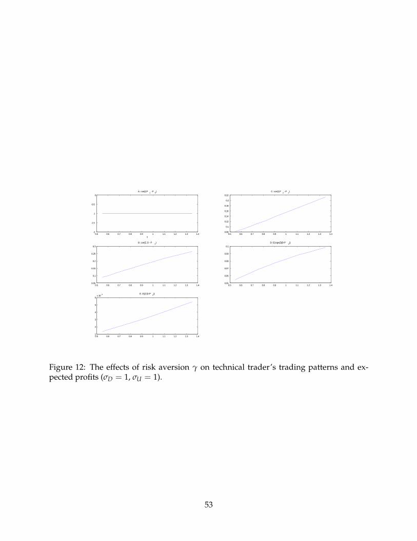
0.5 0.6 0.7 0.8 0.9 1 1.1 1.2 1.3 1.4­2

­1.5

­1

­0.5

0

A: corr(Z,P 1 ­ P 0)

γ0.5 0.6 0.7 0.8 0.9 1 1.1 1.2 1.3 1.4

0.08

0.1

0.12

0.14

0.16

0.18

0.2

0.22

C: corr(Z,P 2 ­ P 1)

0.5 0.6 0.7 0.8 0.9 1 1.1 1.2 1.3 1.40.05

0.1

0.15

0.2

0.25

0.3

B: corr(Z, D ­ P 2)

0.5 0.6 0.7 0.8 0.9 1 1.1 1.2 1.3 1.40.05

0.06

0.07

0.08

0.09

0.1

D: E[sign(Z)(D­P 2)]

0.5 0.6 0.7 0.8 0.9 1 1.1 1.2 1.3 1.41

2

3

4

5

6x 10 ­3 E: E[Z (D­P

2)]

Figure 12: The effects of risk aversion γ on technical trader’s trading patterns and ex-pected profits (σD = 1, σU = 1).

53