NBER WORKING PAPER SERIES

TEACHING THE TAX CODE:EARNINGS RESPONSES TO AN EXPERIMENT WITH EITC RECIPIENTS

Raj ChettyEmmanuel Saez

Working Paper 14836http://www.nber.org/papers/w14836

NATIONAL BUREAU OF ECONOMIC RESEARCH1050 Massachusetts Avenue

Cambridge, MA 02138April 2009

We are extremely grateful to Joe Cresta, David Hussong, Mike Lammers, Scott McBride, Eileen McCarthy,Robert Weinberger, Jeremy White, Bernie Wilson, and the nearly 1,500 tax professionals at H&RBlock for their help in organizing and implementing the experiment. We thank Michael Anderson,David Card, Stefano DellaVigna, Martin Feldstein, Bryan Graham, Caroline Hoxby, Hilary Hoynes,Lawrence Katz, David Laibson, Adam Looney, Erzo Luttmer, Marco Manacorda, Sendhil Mullainathan,Steve Pischke, Karl Scholz, and numerous seminar participants for very helpful comments and discussions.Gregory Bruich and Phillipe Wingender provided outstanding research assistance. Financial supportfrom CASBS, UC-LERF, NSF Grants SES-0645396 and SES-0850631, and the Sloan Foundationis gratefully acknowledged. The views expressed herein are those of the author(s) and do not necessarilyreflect the views of the National Bureau of Economic Research.

© 2009 by Raj Chetty and Emmanuel Saez. All rights reserved. Short sections of text, not to exceedtwo paragraphs, may be quoted without explicit permission provided that full credit, including © notice,is given to the source.

Teaching the Tax Code: Earnings Responses to an Experiment with EITC RecipientsRaj Chetty and Emmanuel SaezNBER Working Paper No. 14836April 2009JEL No. H31,J22

ABSTRACT

This paper tests whether providing information about the Earned Income Tax Credit (EITC) affectsEITC recipients' labor supply and earnings decisions. We conducted a randomized experiment with43,000 EITC recipients at H&R Block in which tax preparers gave simple, personalized informationabout the EITC schedule to half of their clients. Tracking subsequent earnings, we find substantialheterogeneity in treatment effects across the 1,461 tax professionals who assisted the clients involvedin the experiment. Half of the tax professionals, whom we term "compliers", induce treated clientsto increase their EITC refunds by choosing an earnings level closer to the peak of the EITC schedule.Clients treated by complying tax professionals are 10% less likely to have very low incomes than controlgroup clients. The remaining tax preparers generate insignificant changes in EITC amounts but increasethe probability that their clients have incomes high enough to reach the phase-out region. Treatmenteffects are larger for the self-employed, but are also substantial among wage earners, suggesting thatinformation provision induced real labor supply responses. When compared with other policy instruments,information has large effects: complying tax preparers generate the same labor supply response alongthe intensive margin as a 33% expansion of the EITC program, while non-complying tax preparersinduce the same response as a 5% tax rate cut.

Raj ChettyDepartment of EconomicsUniversity of California, Berkeley521 Evans Hall #3880Berkeley, CA 94720and NBERchetty@econ.berkeley.edu

Emmanuel SaezDepartment of EconomicsUniversity of California, Berkeley549 Evans Hall #3880Berkeley, CA 94720and NBERsaez@econ.berkeley.edu

1 Introduction

A central assumption in the literature on tax and transfer policy is that individuals are fully

informed about government policies relevant for their choices. In this paper, we test this

assumption using a �eld experiment with Earned Income Tax Credit (EITC) clients at H&R

Block. The EITC is the largest cash transfer program for low income families in the United

States. One of its major goals is to increase labor supply and earnings among low-income

working households. A prerequisite for achieving this goal is that clients understand how

the EITC program changes their incentives to work. Survey evidence indicates, however,

that the marginal incentive structure of the EITC is not well understood by eligible tax �lers.

Most low-income families have heard about the EITC and know that working is associated

with getting a tax refund check when they �le their taxes. But very few recipients know

whether working more would increase or reduce their EITC amount (Liebman 1998, Romich

and Weisner 2002), perhaps because of the program�s complexity. In addition, individuals get

little feedback about how their behavior a¤ects their EITC refund, as the refund is typically

received several months after the labor supply decisions that determine its size are made.

The lack of information could potentially explain why the EITC induces very small re-

sponses along the intensive margin (hours worked and earnings), despite generating substan-

tial increases in labor force participation (Hotz and Scholz 2003).1 To test this hypothesis,

we conducted a randomized experiment that provided simple information about the EITC to

eligible tax �lers and tracked the e¤ect of this intervention on their subsequent earnings. The

experiment was implemented at 119 H&R Block o¢ ces in the Chicago metro area in 2007.

H&R Block is the largest tax preparer in the U.S., and approximately 40% of its clients are

eligible for the EITC. The experimental population comprised approximately 43,000 tax �lers

who (a) received EITC payments at one of the 119 H&R Block o¢ ces when �ling taxes in

2007 and (b) had one or more dependents. Half of these clients were randomly selected to

receive a two minute explanation about how the EITC works from their �tax professional,�

the H&R Block employee assisting them with their tax returns. Tax professionals were trained

to use three tools to explain the EITC to their clients: a verbal description, a graph showing

the shape of the EITC as a function of earnings, and a table listing the key EITC parameters.

1An alternative hypothesis is that individuals are inelastic on the intensive margin, and that tax �lers choosenot to acquire information about the tax code because they anticipate that it will not a¤ect their behavior.

1

Each client was also given tailored advice emphasizing the implications of his marginal incen-

tives conditional on his location in the EITC schedule. For example, clients in the phase-in

region were told, �It pays to work more!�

We view our treatment as changing perceptions of marginal incentives around the tax �ler�s

current location. Existing survey evidence indicates that most EITC recipients know the size

of their current EITC refund, but undestimate the extent to which the EITC varies with their

earnings. If the information treatment updates perceptions toward the true EITC schedule,

we hypothesize that tax �lers will change their behavior to increase their EITC refunds. Such

behavioral responses should generate a more concentrated earnings distribution around the

peak of the EITC schedule.

We evaluate the e¤ects of the intervention using data from tax returns �led in 2007 (�year

1�) and 2008 (�year 2�). 72% of the clients in the treatment and control groups returned

to H&R Block to �le their taxes in the post-treatment year, allowing us to conduct a panel

study of the e¤ects of the information treatment on earnings. We begin with a simple analysis

of treatment e¤ects in the full sample. We �nd weak evidence (p < 0:1) that year 2 EITC

amounts are higher and the probability of having low income (below $7,000) is lower among

treated clients relative to control clients. We do not detect signi�cant changes in other parts

of the earnings distribution. Recognizing that these comparisons in the full sample could

mask heterogeneous responses, we then examine the heterogeneity of treatment e¤ects across

tax professionals. We expected treatment e¤ects to vary substantially by tax professional for

two reasons. First, the 1,461 tax professionals who implemented the experiment were trained

in a decentralized manner by senior H&R Block employees, leading to variations in training.

Second, a number of tax professionals felt that it was in their clients�best interest to work

and earn more irrespective of the EITC�s incentive e¤ects. These tax professionals framed

the phase-out message as an encouragement to work more because the loss in EITC bene�ts

is relatively small.2

We �rst document that there is signi�cant heterogeneity across tax professionals in mean

treatment e¤ects on EITC amounts using a non-parametric F test. The hypothesis that treat-

ment e¤ects are constant across tax professionals is rejected with p < 0:01. To characterize the

2During focus groups prior to the experiment, several tax professionals argued that clients should always beencouraged to work more because, �you lose $2 of EITC bene�ts for every $10 you earn, but come out aheadby $8 and possibly become eligible for other credits, so it still pays to work.�

2

nature of the heterogeneity, we follow the methodology of Du�o et al. (2006). We divide tax

professionals into two groups: �complying�and �non-complying.� To construct these groups,

we �rst de�ne a simple measure of the concentration of the earnings distribution in year 2 �

the fraction of returning clients with �middle� incomes (between $7,000 and $15,400).3 For

each tax �ler i, we de�ne his tax professional as a �complier� if she has a higher fraction of

other clients (excluding client i) with middle income in the treatment group than the control

group. Intuitively, from the perspective of client i, complying tax professionals are those who

increase the concentration of the earnings distribution for other clients. Critically, because we

exclude client i when de�ning his tax professional�s compliance, there is no correlation between

client i�s outcome and his tax professional�s compliance under the null hypothesis that all tax

professionals have zero treatment e¤ects.

For clients of complying tax professionals, who account for half of the sample, the infor-

mation treatment increases EITC amounts and the concentration of the earnings distribution

signi�cantly. Complying tax professionals raise their treated clients�EITC refund by $68 on

average (p < 0:01), relative to a mean of approximately $2,400. They reduce the probability

that their treated clients have low incomes (below $7,000) by 1.4 percentage points relative to

a base of 15% (p < 0:01). Information provision leads to an especially dramatic accentuation

of bunching around the �rst kink in the EITC schedule among the self-employed. The larger

treatment e¤ects for the self-employed are likely due to greater �exibility and reporting e¤ects

(as there is no third-party reporting of self-employment income). Importantly, however, we

also �nd a signi�cant increase in the concentration of the distribution of wage earnings. Since

it is di¢ cult to manipulate wage and salary income (as it is reported on W-2 forms by employ-

ers), this �nding suggests that the informational intervention induced �real�changes in labor

supply behavior. All of these changes in the distributions of earnings and EITC amounts for

clients of complying tax professionals are visually evident in density plots, and are statistically

signi�cant under non-parametric Kolmogorov-Smirnov tests. In summary, the evidence for

the compliers supports the hypothesis that intensive-margin labor supply responses to the

EITC are attenuated by a lack of information.

For clients of non-complying tax professionals, the information treatment does lot lead to

3The upper threshold of $15,400 is the start of the EITC phase-out range; the lower threshold of $7000 ischosen to divide the remaining interval into two equal-sized bins. We show below that alternative measures ofthe concentration of the earnings distribution yield similar results.

3

signi�cant changes in EITC amounts. However, non-complying tax professionals increase their

treated client�s incomes by $250 (1.5%) on average (p < 0:05). As a result, clients treated by

non-complying tax professionals are 1.7 percentage points more likely to be in the phase-out

range of the EITC schedule (p < 0:05). Based on our discussions with tax professionals, we

speculate that non-compliers may have used the information to simply encourage clients to

aim for a high level of earnings rather than maximize their EITC refunds. Consistent with this

interpretation, we �nd that non-complying tax professionals do not have a signi�cant e¤ect on

reported self-employment income and only a¤ect wage earnings.

The changes in behavior induced by the information treatment are modest in absolute

terms, but substantial when compared with the e¤ects of other policy instruments on intensive

margin labor supply. Previous studies suggest an upper bound on the intensive margin

elasticity of earnings with respect to the net-of-tax rate of 0.25. Using this elasticity, a simple

calibration shows that complying tax professionals generate the same labor supply response

along the intensive margin as a 33% expansion of the EITC. Non-complying tax professionals

increase earnings by an amount equivalent to the response to a 5% tax rate cut. These

calibrations suggest that information and advice are inexpensive ways to in�uence behavior,

as the cost of the treatment was only $5 per EITC claimant in our study.

In addition to the literature on the EITC, which we discuss in greater detail in section

2, our analysis builds on and relates to a rapidly growing literature on the importance of

information and salience for choices in other contexts. Most of these studies show that

providing information has substantial e¤ects on immediate decisions such as enrollment in

pension or health plans, school choices, or grocery purchases (Du�o and Saez 2003, Hastings

and Weinstein 2007, Chetty, Looney, and Kroft 2008, Kling et al. 2008). A few recent studies

have shown that providing incentives can also generate changes in behavior in the longer run.

Jensen (2008) shows that providing information to students in the Dominican Republic on

the returns to schooling reduced dropout rates in subsequent years among some subgroups.

Nguyen (2008) conducts a similar experiment in Madagascar and shows that information on

returns to education increases subsequent test scores.

Our analysis contributes to this literature by showing that information a¤ects labor supply,

which is one of the most important long-term decisions made by households and is central to the

design of tax and transfer policy. Our �ndings reject the common view that intensive margin

4

labor supply behavior is completely inelastic with respect to incentives because of institutional

constraints. Our results also suggest that advice about how one should respond to incentives

has an important in�uence on behavior beyond information itself. Unfortunately, we are

unable to quantify the relative importance of the information and advice channels because

we do not have data on how the treatment a¤ected individuals�priors about the structure

of the EITC.4 Therefore, we view our contribution as an initial exploration showing that

the impacts of tax policies depend on the way in which individuals are taught about the tax

system. In this sense, our results mirror studies of teacher e¤ects (e.g., Rocko¤ 2004): we

show that �teachers�of the tax code a¤ect behavior, but leave the important question of what

makes some people teach and interpret the tax code di¤erently from others to future research.

The remainder of the paper is organized as follows. Section 2 provides background on the

EITC and the literature on the e¤ects of the program. Section 3 describes the experimental

design and data. Results are presented in Section 4. Section 5 presents the calibration

comparing the magnitudes of the information treatment e¤ects to changes in tax policy. We

conclude in section 6 by discussing the implications of our results for future research.

2 Background on the EITC

2.1 Program Structure

The EITC is a refundable tax credit administered through the income tax system. In 2006,

the latest year for which statistics are available, 23 million tax �lers received a total of $44.4

billion in EITC payments (Internal Revenue Service 2008, Table 2.5). Eligibility for the EITC

depends on earnings �de�ned as wage and salary income and self-employment income �and

the number of qualifying children. Qualifying dependents for EITC purposes are relatives who

are under age 19 (24 for full time students) or permanently disabled, and reside with the tax

�ler for at least half the year.5

Figure Ia displays the EITC amount as a function of earnings for single and joint tax

�lers with zero, one, or two or more qualifying dependents in 2007. EITC amounts increase

substantially with the number of dependents, but the shape of the schedule as a function of

4We had originally planned to measure perceptions of marginal incentives using base-year and followupsurveys of the clients involved the experiment, but this component unfortunately was not implemented.

5Only one tax �ler can claim an eligible child; for example, in the case of non-married parents, only oneparent can claim the child.

5

earnings is the same in all three cases. EITC amounts �rst increase linearly with earnings,

then plateau over a short income range, and are then reduced linearly and eventually phased

out completely. Since the EITC amounts for tax �lers with no children dependents are very

small (maximum of $428), we excluded them from our experiment, focusing only on tax �lers

with one or more children.

In the phase-in region, the subsidy rate is 34 percent for taxpayers with one child and

40 percent for taxpayers with two or more children. In the plateau (or peak) region, the

EITC is constant and equal to a maximum value of $2,853 and $4,716 for tax �lers with 1 and

2+ children, respectively. In the phase-out region, the EITC amount decreases at a rate of

15.98% for �lers with 1 child, and 21.06% for those with 2+ children. The EITC is entirely

phased-out at earnings equal to $33,241 and $37,783 for single �lers with 1 and 2+ children,

respectively.6 See IRS Publication 596 (Internal Revenue Service 2007) for complete details

on program eligibility and rules.

2.2 Claiming the EITC: Administrative Procedures

To claim the EITC, families �le an income tax return that includes an EITC schedule between

January 1 and April 15 of the following calendar year. The EITC is received in a single

payment as part of the tax refund shortly after �ling.7

According to the 2004 public use microdata on tax returns, 74% of families receiving the

EITC (with children) use paid tax preparers to �le their returns. The largest company in the

market for paid tax preparation in the United States is H&R Block. H&R Block has about

13,000 o¢ ces located throughout the United States and employs over 100,000 tax professionals

during the tax �ling season. H&R Block currently prepares about 12% of all individual tax

returns in the U.S. A substantial fraction of these returns are for EITC claimants, as over

half of H&R Block�s individual clients have an adjusted gross income (AGI) below $35,000.

To �le their tax returns, clients come to an H&R Block o¢ ce with relevant documents such

as their W-2 wage income forms. The client sits with a �tax professional��the term used to

refer to H&R Block employees who prepare tax returns �in front of a computer running the

6For those who are married and �le jointly, the plateau and phase-out regions of the EITC are extended by$2,000.

7There is an option to receive the EITC in advance during the year through the paycheck, but take-up ofthis option is extremely low (less than 2%). See Government Accountability O¢ ce (2007) and Jones (2008).

6

H&R Block Tax Preparation Software (TPS). TPS consists of a series of screens corresponding

to the various steps in tax return preparation. At each screen, the tax professional asks

questions or inputs information from the forms brought in by the client. The tax preparation

process takes about 30 to 45 minutes to complete for a typical EITC client.

2.3 Existing Evidence and Perceptions of EITC

There is a large empirical literature estimating the e¤ects of the EITC on labor supply and

earnings. Hotz and Scholz (2003) and Eissa and Hoynes (2006) provide comprehensive sur-

veys. A number of studies have found strong evidence that the EITC increases labor force

participation � the extensive margin response.8 However, there is little evidence that the

EITC leads to a change in labor supply for those already in the labor market �the intensive

margin. Most studies �nd no e¤ects of the EITC on hours of work (see e.g., Meyer and Rosen-

baum 1999 and Rothstein 2007). Using tax return data, Saez (2009) �nds clear evidence of

bunching of EITC recipients at the �rst kink of the EITC schedule �where the phase-in ends

and the plateau starts �for recipients reporting self-employment income. However, there is

no bunching for recipients who do not report any self-employment income, who account for

89% of the individuals in our dataset.

The contrast between the strong responses along the extensive margin and small or zero

responses along the intensive margin could be explained by a lack of information about the

structure of the EITC (Liebman 1998, Hotz and Scholz 2003, p. 182).9 To respond along

the extensive margin, families only need to know that working is associated with a large tax

refund. In contrast, responding along the intensive margin requires knowledge about the

non-linear marginal incentives created by the three ranges of the EITC displayed in Figure Ia.

Surveys of low income families and in-depth interviews of EITC claimants show that there is

widespread knowledge about the EITC�s existence, but little knowledge about the structure

of the EITC (Ross Phillips 2001, Olson and Davis 1994, Romich and Weisner 2002, Smeeding,

8See e.g., Eissa and Liebman (1996), Meyer and Rosenbaum (2001). Eissa and Hoynes (2004) presentcomplementary evidence of extensive-margin responses in the opposite direction: the labor force participationrate of married women in the phase-out region of the schedule falls slightly when the EITC was expanded. Weexpect that this extensive-margin response has a small impact on our results because 91% of the tax �lers inour sample are single.

9The bunching at the �rst kink for those who report self-employment income shows that some tax �lers knowabout the EITC structure, but the lack of bunching in the rest of the population suggests that such knowledgeis limited to this small group.

7

Ross Phillips, and O�Connor 2002, Maag 2005). These interviews indicate that 60-90% of

low income families have heard about the EITC and know that it is a tax refund for working.

However, less than 5% of these families know about the non-linear �bell shape�of the EITC

as a function of earnings and the location of the kink points.10

The lack of knowledge about the EITC�s structure is striking given that the program

parameters have been quite stable for over a decade. However, it is not surprising in view of the

information currently available about the program. To our knowledge, prior to our experiment,

the graphical depiction of the EITC schedule shown in Figure Ia could only be found in

academic papers. O¢ cial Internal Revenue Service publications provide tables that show

exact EITC amounts as a function of income and other characteristics, but do not summarize

the EITC phase-in, peak, and phase-out structure in a transparent way. For legal reasons, the

IRS only distributes comprehensive documents that cover all possible contingencies, making

it impossible to highlight the features of the tax code most relevant for a given taxpayer.11

In addition, none of the existing commercial tax preparation software describes the EITC

structure or marginal incentives explicitly.

We conclude from the existing literature that most EITC recipients know the value of their

current EITC refund amount, but do not think about the slope of the EITC schedule when

making marginal earnings decisions. Hence, the average individual�s perception of the EITC

schedule is locally �atter than the actual schedule. More precisely, let EITCp(z) denote

the individual�s perceived EITC refund at an earnings level of z and EITC(z) the actual

EITC refund at that level of earnings. Let sp(z) denote the perceived local slope of the

EITC schedule and s(z) the actual slope. The existing survey evidence suggests that the

representative individual with initial earnings z0 perceives the relationship between earnings

z and his EITC refund to be

EITCp(z) = EITC(z0) + (1 + sp(z))(z � z0) (1)

where jsp(z)j < js(z)j. Figure Ib illustrates the perceived budget constraint in (1) for two tax

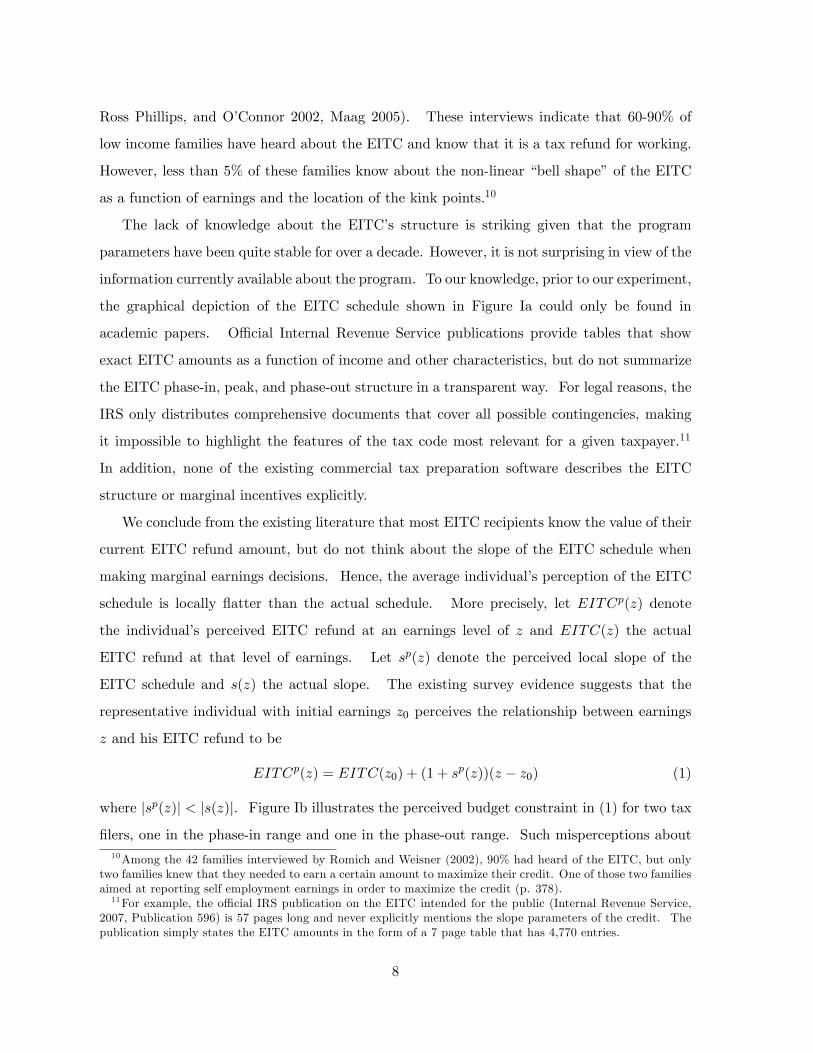
�lers, one in the phase-in range and one in the phase-out range. Such misperceptions about10Among the 42 families interviewed by Romich and Weisner (2002), 90% had heard of the EITC, but only

two families knew that they needed to earn a certain amount to maximize their credit. One of those two familiesaimed at reporting self employment earnings in order to maximize the credit (p. 378).11For example, the o¢ cial IRS publication on the EITC intended for the public (Internal Revenue Service,

2007, Publication 596) is 57 pages long and never explicitly mentions the slope parameters of the credit. Thepublication simply states the EITC amounts in the form of a 7 page table that has 4,770 entries.

8

marginal incentives motivate our question of whether improving knowledge (updating sp(z))

could amplify the impacts of the EITC on intensive-margin labor supply.12

3 Experimental Design

We implemented the information-provision experiment in 119 H&R Block o¢ ces in the Chicago

metropolitan area during the 2007 tax �ling season (January 1 to April 15). Clients at

these o¢ ces who received an EITC with at least one eligible child were randomly assigned

into the treatment or control group. Assignment was based on the last 2 digits of the Social

Security Number of the primary �ler. The probability of treatment assignment was 50 percent.

The control group followed the standard tax preparation procedure using the TPS software

described above. In the standard preparation procedure, a screen noti�es the tax �ler of his

EITC amount if he is eligible for the EITC. This screen does not explain the structure of the

EITC.

The new EITC information materials delivered by tax professionals to clients in the treat-

ment group were developed in a series of steps. We began by interviewing 12 single mothers

with recent work experience in the welfare o¢ ce of San Francisco county in early October

2006. All 12 single mothers had �led tax returns in the past and almost all had heard about

the EITC, but none knew about or had seen the graphical depiction of how the EITC varies

with earnings. The interviewees found the graphical presentation of the EITC reasonably easy

to understand and felt that it made the key features of the EITC very salient. Furthermore,

most of the individuals recognized the value of this information for their work decisions and

found the take-home messages sensible.13

We re�ned the information materials in a focus group with 15 experienced H&R Block

tax professionals and local managers in the Chicago area in late October 2006. Finally,

H&R Block�s internal sta¤ and legal team edited and approved all the materials used in

the experiment. The process described below is the �nal procedure that resulted from the

collaborative e¤ort between the researchers and H&R Block. Note that in all o¢ cial tax12There is similar evidence that people are not fully informed about many other aspects of income tax

schedules. See Fujii and Hawley (1988) for evidence from the United States, Brown (1968) for the UnitedKingdom, Bises (1990) for Italy, and Brannas and Karlsson (1996) for Sweden.13For example, one of the interviewees suggested that we visit her housing complex to distribute this infor-

mation more widely, because her neighbors and friends would �nd it useful in making overtime and part-timework decisions.

9

forms as well as in H&R Block materials, the EITC is referred to as the EIC (Earned Income

Credit). We follow this convention in the information treatment materials described below.

3.1 Information Treatment Procedure

For the treatment group, two special �EIC information�screens are displayed automatically in

TPS at the end of the tax preparation process.14 The �rst screen prompts the tax professional

to begin the EIC explanation they were trained to provide and introduces the client to the

information outreach program. This introductory screen is shown in Appendix Exhibit I(a)

for the case of a single �ler with two or more dependents, the case on which we focus below

for concreteness. The screen displays the EIC amount the tax �ler is getting and describes

the goal of the outreach e¤ort, namely to help the client understand how the EIC depends on

earnings. The second EIC information screen is displayed in Appendix Exhibit I(b) for a tax

�ler in the increasing range of the EIC. This screen provides the key EIC information relevant

to the tax �ler�s case, which the tax professional uses to explain the program to the client.

The central element of the explanation procedure is an �EIC handout� paper form that

the tax professional �lls out with the client and uses as a visual aid to explain the program.

There are four EIC handouts based on the tax �ler�s marital status and dependents: single

vs. joint �ler and one vs. two or more dependents. Exhibit I shows the EIC handout for the

case of a single �ler with two or more dependents. The tax professional uses the information

on the computer screen to �ll in the blanks on the form in the following four steps.

First, the tax professional �lls in the income that the client earned in 2006 and the corre-

sponding EIC amount the client is receiving. Second, the tax professional draws a dot on the

graph illustrating the client�s location on the schedule. He then uses the graph to explain the

link between earnings and the EIC amount.

In the third step, the tax professional circles the range of the schedule that the client is in

�increasing, peak, or decreasing �and provides some advice corresponding to that range. In

the increasing range, the take-home message is �Suppose you earn $10 an hour, then you are

really making $14 an hour. It pays to work more!� In the peak range, the message is �Your

14This screen appears after all the client�s tax information has been entered and the tax refund and liabilityhave been calculated. We show below that there is no di¤erence in base year earnings across control andtreatments groups, implying that treated tax �lers did not go back and change their reported earnings in thebase year after getting the EIC information.

10

earnings are maxing-out the EIC amount.� In the decreasing range, the message is �If you

earn $10 more, your EIC is reduced by $2.10. Earning more reduces your EIC, but you may

qualify for additional tax credits.�

The decreasing range message deliberately downplays the work disincentive created by

the EITC in the phaseout region. The advice took this form because many managers and

tax professionals at H&R Block felt strongly that it was in the best interest of tax �lers to

work and earn more. Indeed, many tax professionals pitched the message verbally as �You

lose $2 of your EIC credit when you earn $10 more, but you still come out ahead by $8 and

potentially become eligible for other credits, so working more pays o¤.�15 The fact that some

tax professionals advised clients to aim for a high level of earnings �irrespective of the EITC�s

e¤ect on incentives �appears to have important e¤ects on the results, as we will see below.

In the fourth step, the tax professional circles the relevant range in the table which displays

the exact parameters for the EITC. This table provides an alternative method of showing

exactly how much the client can change his earnings before crossing the threshold for the

next range. Tax professionals were trained to spend the most time on whichever of the three

methods the client appeared to understand best �the verbal, graphical, or tabular descriptions.

After this information explanation is provided and the tax return process is completed,

TPS automatically prints an �EIC printout�page that reproduces the information �lled out

in the handout. Appendix Exhibit II displays an example of the EIC printout. This page

is printed at the same time as the tax return and inserted at the top of the packet given to

the client to take home. The client is reminded by the tax professional that this information

may prove useful when making earnings-related decisions later in the year. The purpose of

the printout is to present the EITC information in a clean, accurate format. The temporary

handout used to explain the program is kept by the tax professional.

Finally, to reinforce the treatment, H&R Block sent a letter summarizing the EITC in-

formation to all treatment-eligible clients in August 2007. Appendix Exhibit III displays an

example of this letter.

As with most provisions of the tax code, EITC ranges are mechanically indexed for in�a-

tion and therefore di¤er slightly across the base year and subsequent year. Since our goal

15 In some cases, other credits such as the non-refundable portion of the child tax credit do indeed increasewith earnings in the EITC phaseout range, mitigating the implicit tax on work. We chose not to explain allaspects of the tax system in our information handout in the interest of simplicity.

11

was to inform tax �lers about the EITC parameters relevant for their subsequent labor sup-

ply decisions, the table and graph display the EITC parameters for 2007 earnings and the

corresponding EITC that would be received when �ling in 2008 (the post-treatment year).

The classi�cation of tax �lers into the 3 groups �increasing, peak, and decreasing �was also

based on the 2007 EITC parameters. As a result, a tax �ler who was at the very beginning

of the peak range would actually be presented with the increasing scenario that would apply

were he to have the same nominal income in 2007. Similarly, a tax �ler at the very beginning

of the decreasing range would be presented with the peak scenario. Since the IRS in�ation

rate applied from tax year 2006 to 2007 was relatively small (3.9%), only 4% of taxpayers

were located at a point where their current range di¤ered from their predicted range for the

following year. Note that the phase-in and phase-out rates were unchanged across the years.

3.2 Tax Professional Behavior

The e¤ects of the experiment depend critically on the knowledge and behavior of the tax

professionals. There were 1,461 tax professionals involved in the experiment, each of whom

had 29 clients in our sample on average (including treatment and control). We trained

approximately 100 �o¢ ce leaders�(senior tax professionals) in November 2006 ourselves, who

then trained the rest of the tax professionals during December 2006. The training described

the general goal of the outreach e¤ort, why the experimental design required giving information

to only half the clients, and explained the changes to the TPS system that would be introduced.

A series of case studies with hypothetical clients were used to illustrate various scenarios and

how standardized explanations should be provided in the four steps.16 Field observations

in January 2007 con�rmed that the EIC information screens and printouts were working as

planned and that tax professionals were implementing the experiment as trained.

In pilot sessions, we found that a minimum time of two minutes was required for a coherent

explanation of the EITC. To give tax professionals an incentive to administer the information

treatment carefully to eligible clients, each tax professional was o¤ered $5 for each eligible client

with whom they spent at least two minutes on the EIC information screens (with time tracked

by the software). If the tax professional attempted to exit the information screens before

two minutes elapsed, the TPS system displayed a warning, �Does your client understand the

16The powerpoint slides and case studies used for training are available from the authors upon request.

12

explanation of how the EIC impacts their tax return?� The system then allowed the tax

professional to go back and continue his explanation, resuming the two minute clock. Tax

professionals who spent less than two minutes on the information screens did not receive

any compensation for that client. Figure II displays a histogram of seconds spent by tax

professionals on the EITC screens. There is clear spike at 120 seconds (denoted by the vertical

line), showing that most tax professionals understood and responded to the compensation

structure. The average time spent on the information screens conditional on reaching 120

seconds is 3.5 minutes.

Overall, 73% of tax �lers whom we intended to treat were treated for at least two minutes.

A substantial fraction of the variance in compliance rates is explained by o¢ ce �xed e¤ects,

presumably due to variations in training. Most o¢ ces had very high compliance. However,

one large o¢ ce had a two-minute treatment rate of 6%, 11 percentage points below the next

lowest o¢ ce. We believe this exceptionally low treatment rate arose from a failure to hold the

planned training sessions. Since the treatment was e¤ectively not implemented at this o¢ ce,

we exclude it from the analysis below.17

The decision to o¤er a 2+ minute EITC explanation to eligible clients may have depended

on the client�s interest in the information. Since a client�s interest is not random, we fol-

low standard practice in the experimental literature and estimate �intent-to-treat� e¤ects �

comparing outcomes of those eligible and ineligible to receive the information explanation.

To supplement the statistics on compliance rates, we directly assessed the tax professionals�

reactions to the experiment using a survey of the tax professionals at the end of the tax season.

See Appendix Exhibit IV for the survey instrument. To obtain candid responses, the surveys

identi�ed o¢ ces but not individual tax professionals within those o¢ ces. 78% of the 119

o¢ ces sent back completed surveys, yielding a total of 785 survey responses. 88% of the

tax professionals who responded to the survey thought that the EITC information should

be o¤ered again in the future. 81% of surveyed tax professionals thought that the EITC

experiment pilot helped their own understanding of how the EITC credit works. This shows

that our outreach e¤ort did provide new information about the structure of the EITC beyond

what is normally provided in the tax preparation procedure at H&R Block.18 When asked

17 Including the o¢ ce does not change our qualitative results but, unsurprisingly, slightly reduces the magni-tude and precision of the estimates.18Tax professionals who went through our training process may have o¤ered better explanations on the EITC

13

about client interest, 37% of tax professionals said that �most� (>75%) of their clients were

interested in the information explanation. 38% of the tax professionals said that �many�

(25 to 75%) clients were interested, while 25% of tax professionals felt that few (<25%) of

their clients were interested. We conclude from these surveys that most tax professionals

were enthusiastic about the experiment and thought it was a valuable service for their clients,

suggesting that the information treatment was implemented satisfactorily.

3.3 Hypothesis

Our general hypothesis is that the provision of information and advice by tax professionals

induces clients to change their earnings behavior. More speci�cally, tax professionals who

implement our information treatment as intended should update their clients� perceptions

toward the true EITC schedule, shifting sp toward s in equation (1).19 This change in

perceptions of marginal incentives rotates the perceived budget set as shown in Figure Ib,

generating substitution e¤ects but no income e¤ects. Such substitution e¤ects should increase

earnings for tax �lers who would have been in the phase-in range absent the treatment, leave

earnings unchanged for those in the peak, and decrease earnings for tax �lers in the phase-out.

One natural method of testing this prediction is to ask whether incomes rise for tax �lers

who were in the phase-in region in the base year and fall for those in the phase-out in the base

year. This strategy e¤ectively uses base-year income as a proxy for the (counterfactual) level of

year 2 income absent the treatment. The problem with this approach is that incomes are very

unstable across years for low-income individuals. The standard deviation of residual income

growth in our sample is 62% after controlling for a cubic in base-year income, self-employment

status, and number of dependents. Because of this high level of income volatility, many tax

�lers who are initially in the phase-in region move to the peak or phase-out regions in the

next year even in the control group. The inability to predict tax �lers�locations in the EITC

schedule in the post-treatment year makes it di¢ cult to sign the direction in which earnings

to tax �lers in the control group as well. To minimize such contamination e¤ects, we emphasized repeatedlyin training that it was critical not to give any extra information to the clients who were not selected fortreatment for the purpose of the study. Any remaining contamination e¤ects would attenuate our treatmente¤ect estimates.19A key limitation of the present study is that we can only speculate about how our treatment changed

baseline perceptions because we were unable to collect data on prior beliefs. As a result, we are only able totest the broad null hypothesis that information and advice do not a¤ect behavior. Testing sharper hypothesesabout the link between changes in priors and changes in behavior would be a valuable direction for future work.

14

should change for a given tax �ler.

In view of the instability problem, we take an alternative approach to testing for substitu-

tion e¤ects that does not rely on base year income as a proxy for counterfactual year 2 income.

Our strategy is to compare the unconditional distributions of post-treatment earnings and

EITC amounts in the treatment and control groups. In particular, we test two hypotheses:

(1) the distribution of year 2 earnings for treated clients in more concentrated around the

peak of the EITC schedule (i.e., treated clients are less likely to have very low and very high

incomes); and (2) treated clients get larger EITC refunds in year 2 on average than control

clients.

4 Results

Our analysis of the experimental results is based on anonymous statistical compilations pre-

pared by H&R Block in accordance with applicable laws. These compilations were constructed

from data extracted from tax returns �led in 2007 and 2008 and from supplemental information

collected by H&R Block during the implementation of the experiment in 2007.

4.1 Descriptive Statistics

Table I presents descriptive statistics for the treatment and control groups. The means of

all of the base year variables are similar in the treatment and control groups. None of the

mean di¤erences are signi�cant at the 5 percent level, con�rming that randomization was

successful. The mean income in the base year (year 1) in the full sample is $16,600. Income

is the sum of wage earnings and self-employment income. Average wage earnings are $15,900.

Average self-employment income is $700, and 11% of tax �lers report positive self-employment

income.20 The mean EITC amount in the base year is $2,480. About 60% of the claimants

have two or more dependents in the base year, and 63% report two or more dependents in

the post-treatment year. There is no di¤erential change in the number of dependents in the

control and treatment groups, indicating that the treatment did not induce tax �lers to change

the number of dependents they claim.21 The vast majority of the individuals in the sample

20More precisely, positive self-employment income was measured as having positive self-employment taxes. Noself-employment taxes are due if self-employment income is below $400. 11% of tax �lers have self-employmentincome above $400.21This is consistent with the fact that information on how the EITC varies with the number of children was

not provided.

15

are single.

In order to examine distributional outcomes, throughout the paper we divide the income

distribution into three bins: low incomes (below $7000), middle incomes ( $7000 to $15,400),

and high incomes (above $15400). The upper threshold of $15,400 is the start of the EITC

phase-out range; the lower threshold of $7000 is chosen to divide the remaining interval into

two equal-sized bins. By this classi�cation, 14% of the sample is �low income�, 33% is �middle

income�, and 51% is �high income.�

The bottom row of Table I shows the fraction of clients who returned to H&R Block in

year 2. The average return rate is around 72%. The return rate is 0.85% lower in the

treatment group, a small but marginally signi�cant di¤erence. We explore the pattern of

return rates further in Figure III, which plots mean return rates by $1,000 base-year earnings

bins in the treatment and control groups. The average return rates track each other very

closely, showing that there are no systematic patterns of di¤erential attrition by base year

income. In addition, there are no signi�cant di¤erences between the treatment and control

groups in the base-year variables in Table I for the subsample of clients who return. In view

of this evidence, we believe that the comparisons between the treatment and control groups

which follow are unlikely to be contaminated by selective attrition.

4.2 Full Sample Results

We begin our empirical analysis by comparing the year 2 EITC amount and earnings dis-

tributions in the treatment and control groups. Row 1 of Table II reports p values from

non-parametric Kolmogorov-Smirnov (KS) tests for di¤erences in the empirical distributions

of several variables in the full sample. Column 1 shows that there is a marginally signi�cant

di¤erence in the distribution of year 2 EITC amounts between the treatment and control group

(p = 0:07). Column 2 shows that the di¤erence between the income distributions is statisti-

cally insigni�cant.22 Visual examination of the empirical income and EITC distributions (not

reported) reveals no sharp di¤erences between the treatment and control groups, consistent

with the results of the KS tests.

Next, we estimate treatment e¤ects using OLS regressions of the form

yi = �+ �treati + Xi + "i (2)

22We discuss columns 3 and 4 of this table in section 4.4.

16

where yi is a year 2 outcome, treati is de�ned as an indicator for being eligible for the treatment,

and Xi is a vector of year 1 covariates. The coe¢ cient of interest, �, can be interpreted as

an intent-to-treat estimate. Table III presents estimates of � for various outcomes. The

columns of Table III consider di¤erent outcomes or sets of covariates, while the rows consider

di¤erent subsamples. Each coe¢ cient listed in the table is from a separate regression. We

report standard errors clustered by tax professional in parentheses and t-statistics in square

brackets.23

The dependent variable in columns 1 and 2 is the di¤erence between the client�s EITC

amount in the post-treatment and pre-treatment years. Columns 3-6 measure changes in

the income distribution. The dependent variable in columns 3 and 4 is an indicator for

having �middle income� ($7,000 to $15,400) in year 2. In column 5, it is a �low income�

indicator (<$7; 000) and in column 6 a �high income�indicator (>$15; 400). Finally, column

7 considers the mean change in earnings from year 1 to year 2. In columns 2 and 4-7, we

include the following vector of base year covariates (X): earnings, earnings squared, wage

earnings, indicator for married �ling jointly, and number of children (1 vs. 2 or more).

Row 1 of Table III shows treatment e¤ect estimates for the full sample (rows 2-5 are dis-

cussed in the next section). Consistent with the non-parametric tests above, we do not detect

robust di¤erences in EITC amounts or earnings distribution across the treatment and control

groups. Most of the coe¢ cients are small and statistically insigni�cant. The two variables for

which there is some evidence of a treatment e¤ect are the change in EITC amounts ($24 higher

on average in the treatment group) and the likelihood of low income (0.6 percentage points

lower in the treatment group). These e¤ects are marginally signi�cant (p < 0:1). Overall,

we conclude that the full sample does not exhibit sharp di¤erences between the treatment and

control groups.

4.3 Heterogeneity in Treatment E¤ects Across Tax Professionals

As described above, we expect substantial heterogeneity in treatment e¤ects across the 1,461

tax professionals involved in the experiment because of variations in training and willingness

to convey the take-home messages we proposed. Such heterogeneity across tax professionals

23The number of observations is the same for all regressions in each row and is reported only once per row insquare brackets.

17

could potentially be masked in the full sample. We begin our analysis of treatment e¤ect

heterogeneity across tax professionals using an F test. Let i = 1; :::; N index clients and

p = 1; :::; P index tax professionals. Let �EITCi denote the change in the EITC amount

(from year 1 to year 2) for client i. Let tpi;p denote an indicator variable for whether client i

is served by tax professional p and treati denote an indicator for whether the client is in the

treatment group. We implement the F test using a regression of the following form:

�EITCi =PXp=1

�ptpi;p +PXp=1

�ptreati � tpi;p + "i

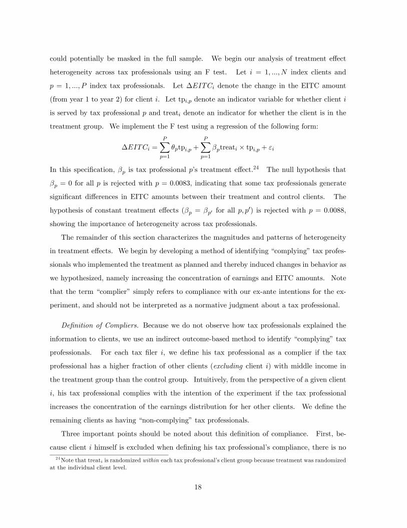
In this speci�cation, �p is tax professional p�s treatment e¤ect.24 The null hypothesis that

�p = 0 for all p is rejected with p = 0:0083, indicating that some tax professionals generate

signi�cant di¤erences in EITC amounts between their treatment and control clients. The

hypothesis of constant treatment e¤ects (�p = �p0 for all p; p0) is rejected with p = 0:0088,

showing the importance of heterogeneity across tax professionals.

The remainder of this section characterizes the magnitudes and patterns of heterogeneity

in treatment e¤ects. We begin by developing a method of identifying �complying�tax profes-

sionals who implemented the treatment as planned and thereby induced changes in behavior as

we hypothesized, namely increasing the concentration of earnings and EITC amounts. Note

that the term �complier�simply refers to compliance with our ex-ante intentions for the ex-

periment, and should not be interpreted as a normative judgment about a tax professional.

De�nition of Compliers. Because we do not observe how tax professionals explained the

information to clients, we use an indirect outcome-based method to identify �complying�tax

professionals. For each tax �ler i, we de�ne his tax professional as a complier if the tax

professional has a higher fraction of other clients (excluding client i) with middle income in

the treatment group than the control group. Intuitively, from the perspective of a given client

i, his tax professional complies with the intention of the experiment if the tax professional

increases the concentration of the earnings distribution for her other clients. We de�ne the

remaining clients as having �non-complying�tax professionals.

Three important points should be noted about this de�nition of compliance. First, be-

cause client i himself is excluded when de�ning his tax professional�s compliance, there is no24Note that treati is randomized within each tax professional�s client group because treatment was randomized

at the individual client level.

18

correlation between client i�s outcome and his tax professional�s compliance under the null

hypothesis that all tax professionals had zero treatment e¤ects. A proof of this simple result

is given in the Appendix. To see the intuition, suppose a placebo treatment is randomly

assigned to individuals, with no information provided to anyone. De�ne �complying� and

�non-complying� tax professionals for each client as above. In this case, �complying� and

�non-complying�are e¤ectively randomly assigned, as the placebo treatment has no impact on

year 2 earnings. Therefore, the sample of clients with a �complying�tax professional are sim-

ply a random subsample of the initial sample. Within that subsample, individual treatment

status remains randomly assigned and hence should have no impact on outcomes. Hence, we

would detect zero treatment e¤ects within the subsample of clients served by complying (or

non-complying) tax professionals if all tax professionals have zero treatment e¤ects.25

Second, the de�nition of complying tax professionals is client-speci�c, as excluding a par-

ticular client might shift a given tax professional from the complying to the non-complying

category (and vice-versa). This creates a correlation in the error terms for clients served by

the same tax professional, as similar clients will tend to either all be excluded or included in

the �complying�group. We account for this problem by clustering all standard errors by tax

professional. To check this method of computing standard errors, we also calculate p values for

each regression we run using the following permutation method. We �rst generate a placebo

treatment randomly (with 50% probability) and recompute complying vs. non-complying tax

professional status for each tax �ler using this placebo treatment variable. We then estimate

the regression speci�cation using the placebo treatment in lieu of the actual treatment to

obtain a placebo coe¢ cient. This process is repeated 2000 times to generate an empirical

distribution of placebo coe¢ cients. Finally, the permutation-based p value is computed using

the location of the actual treatment e¤ect in the empirical cdf of the placebo coe¢ cients. We

�nd that the di¤erence between the permutation-based p values and the p values from regres-

sions with clustered standard errors is less than 0:02 for every regression coe¢ cient reported

below.26 This placebo analysis also con�rms that our method of identifying complying tax

professionals does not induce any arti�cial correlations between treatment and outcomes.

25The di¤erences between the means of the base year variables in the treatment and control groups areinsigni�cant within the subsamples of clients served by complying and non-complying tax professionals, as inTable I.26Since there is no natural counterpart to clustering for the Kolmogorov-Smirnov tests in Table II, we report

the permutation-based p values in that table.

19

Third, the de�nition of compliance above is one of many possible de�nitions. In our

baseline analysis, we de�ne compliance based on the middle income indicator because it pro-

vides a simple, non-parametric way of measuring changes in the concentration of the earnings

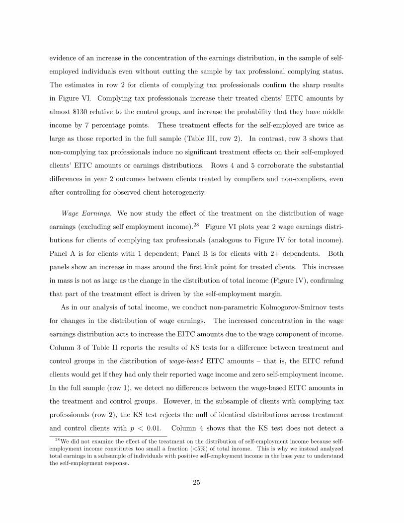
distribution. In section 4.5, we show that similar results are obtained when compliance is

de�ned based on treatment e¤ects on EITC amounts, which is e¤ectively a smoother measure

of changes in the concentration of the income distribution. We also show that controlling

for base year characteristics of clients when classifying tax professionals and using continuous

measures of the degree of compliance instead of a binary classi�cation yields similar results.

Graphical Evidence and Non-Parametric Tests. Figure IV plots the density of post-

treatment income for clients with complying tax professionals. The dashed blue line is for

clients in the control group and the solid red line is for clients in the treatment group. Panel

A considers clients with 1 dependent and Panel B those with 2+ dependents. The red vertical

lines mark the cuto¤s for the phase-in and phase-out regions for each case, and the EITC

schedule is shown in orange. In both panels, there is greater mass in the treated group near

the �rst kink point of the EITC schedule than there is in the control group. Conversely, there

are fewer treated clients in the phase-out range.

The increased concentration in the earnings distribution increases EITC amounts for

treated clients. This result is con�rmed by the KS test reported in the second row of Column

1 of Table II. The null hypothesis that there are no di¤erences in EITC amounts between

treated and control clients is rejected with p < 0:01 for complying tax professionals. The KS

test does not detect a statistically signi�cant di¤erence between the income distributions in the

treatment and control groups for complying tax professionals, as shown in Column 2. This is

not surprising, as the KS test has greater power in detecting uniform shifts in the distribution

relative to changes in concentration.27 We show below that parametric estimators do show

highly signi�cant di¤erences between the income distributions in Figure IV.

Figure V compares the earnings distributions for clients of complying tax professionals with

those for clients of non-complying tax professionals. Panel A is for clients in the treatment

group and Panel B is for the control group. Both panels show the 1 dependent case; results

27The KS test statistic is the maximum absolute di¤erence between the empirical cdf�s. Therefore, a uniformshift generates a large KS statistic than an increase in concentration, which creates a rightward shift at thebottom and a leftward shift at the top, making the two cdf�s cross.

20

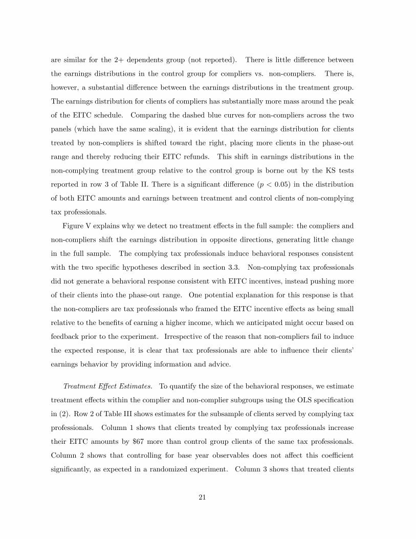
are similar for the 2+ dependents group (not reported). There is little di¤erence between

the earnings distributions in the control group for compliers vs. non-compliers. There is,

however, a substantial di¤erence between the earnings distributions in the treatment group.

The earnings distribution for clients of compliers has substantially more mass around the peak

of the EITC schedule. Comparing the dashed blue curves for non-compliers across the two

panels (which have the same scaling), it is evident that the earnings distribution for clients

treated by non-compliers is shifted toward the right, placing more clients in the phase-out

range and thereby reducing their EITC refunds. This shift in earnings distributions in the

non-complying treatment group relative to the control group is borne out by the KS tests

reported in row 3 of Table II. There is a signi�cant di¤erence (p < 0:05) in the distribution

of both EITC amounts and earnings between treatment and control clients of non-complying

tax professionals.

Figure V explains why we detect no treatment e¤ects in the full sample: the compliers and

non-compliers shift the earnings distribution in opposite directions, generating little change

in the full sample. The complying tax professionals induce behavioral responses consistent

with the two speci�c hypotheses described in section 3.3. Non-complying tax professionals

did not generate a behavioral response consistent with EITC incentives, instead pushing more

of their clients into the phase-out range. One potential explanation for this response is that

the non-compliers are tax professionals who framed the EITC incentive e¤ects as being small

relative to the bene�ts of earning a higher income, which we anticipated might occur based on

feedback prior to the experiment. Irrespective of the reason that non-compliers fail to induce

the expected response, it is clear that tax professionals are able to in�uence their clients�

earnings behavior by providing information and advice.

Treatment E¤ect Estimates. To quantify the size of the behavioral responses, we estimate

treatment e¤ects within the complier and non-complier subgroups using the OLS speci�cation

in (2). Row 2 of Table III shows estimates for the subsample of clients served by complying tax

professionals. Column 1 shows that clients treated by complying tax professionals increase

their EITC amounts by $67 more than control group clients of the same tax professionals.

Column 2 shows that controlling for base year observables does not a¤ect this coe¢ cient

signi�cantly, as expected in a randomized experiment. Column 3 shows that treated clients

21

are 2.9 percentage points more likely to report middle income than control clients within

the sample of complying tax professionals. Column 4 shows that this estimate is also not

signi�cantly a¤ected by controlling for base year characteristics. Columns 5 and 6 show that

treated clients are less likely to have both low incomes and high incomes, con�rming that

the complying tax professionals use the information to push clients toward the peak. The

e¤ect on low incomes is particularly large: the probability of having an income below $7,000

falls by 1.5 percentage points relative to a base of 15%. Column 7 shows that the treatment

does not induce a signi�cant change in mean earnings from year 1 to year 2. The �nding is

consistent with an increase in concentration rather than a shift of the earnings distribution,

and underscores the importance of investigating moments beyond means when budget sets are

non-linear (Bitler, Gelbach, and Hoynes 2006).

Row 3 considers the non-complying tax professionals. Clients given the information treat-

ment by these tax professionals experience a statistically insigni�cant reduction of $32 (column

2) in their EITC amounts relative to their peers in the control group. This is because non-

complying tax professionals reduce their treated clients�probability of having middle income

by 2.15 percentage points (column 4), shifting clients away from the region of the EITC sched-

ule where refunds are maximized. Non-compliers increase the probability that their treated

clients locate in the phase-out region of the schedule: the probability of having high income

is 1.7 percentage points higher in the treatment group relative to the control (column 6). As

a result, the earnings of treated clients rise by $250 more on average than control clients of

non-compliers (column 7). These results are consistent with the density plots in Figure V:

non-compliers shift the earnings distribution to the right and increase the likelihood of high

incomes. The mean of the coe¢ cients in rows 2 and 3 roughly corresponds to the coe¢ cients

in row 1, explaining why we do not detect clear treatment e¤ects in the full sample.

Finally, in rows 4 and 5, we compare the treatment e¤ects for complying and non-complying

tax professionals to test whether the estimates reported in rows 2 and 3 are statistically

distinguishable. We estimate a model analogous to (2) on the full sample, interacting all

the variables with an indicator for having a complying tax professional. Row 4 reports the

coe¢ cient on the interaction of the treatment and complier indicators, which is simply the

di¤erence in the coe¢ cients reported in rows 3 and 4. Under the null hypothesis of zero

treatment e¤ects for all tax professionals, this �di¤erence in di¤erence�estimate would be zero.

22

Contrary to the null, all of the coe¢ cients reported in row 4 are statistically signi�cant. Clients

treated by complying tax professionals experience approximately a $90 larger increase in their

EITC refund on average relative to clients treated by non-complying tax professionals. Clients

treated by compliers are also substantially more likely to have middle incomes. Finally, clients

treated by compliers have on average $420 lower growth in earnings than clients treated by non-

compliers. These results highlight the substantial amount of treatment e¤ect heterogeneity

across tax professionals.

The heterogeneity in treatment e¤ects that we have documented could come from two

potential sources. One natural interpretation �which is the one we have suggested thus far

� is that tax professionals implemented the information treatment in di¤erent ways, leading

to di¤erent outcomes. An alternative view is that the variation in treatment e¤ects is not

caused by di¤erences in tax professionals�behavior but instead by variations in the set of clients

that di¤erent types of tax professionals served. Our experiment randomized the information

treatment within tax professional but did not randomize clients across tax professionals.

In row 5 of Table III, we explore the source of the treatment e¤ect heterogeneity by adding

interactions of the vector of base year controls with the treatment dummy to the speci�cations

in row 4. In this speci�cation, the coe¢ cient on the interaction of the treatment and complier

indicators can be interpreted as the e¤ect of having a complying tax professional, holding

�xed observable base year characteristics. We �nd that all seven coe¢ cients in row 5 are very

similar to the corresponding coe¢ cients in row 4, indicating that the heterogeneity in treatment

e¤ects is not driven by observable heterogeneity in client characteristics. The heterogeneity in

treatment e¤ects could, however, be driven by unobservable heterogeneity in treatment e¤ects

across clients. For instance, suppose clients sort across tax professionals in a way that is

correlated with their knowledge of the EITC. Then the heterogeneity in treatment e¤ects

across tax professionals could be driven by heterogeneity in clients�knowledge. Complying

tax professionals could be those who serve clients with ��at� priors as in Figure Ib, while

non-complying tax professionals could be those whose clients think that the phase-out rate is

higher than it actually is. Note that such client heterogeneity explanations require substantial

sorting of clients purely on unobserved characteristics. While we cannot rule out such sorting,

we believe that the sharp di¤erences in treatment e¤ects across complying and non-complying

tax professionals are more likely to be driven by the tax professionals themselves.

23

Importantly, regardless of the source of heterogeneity, the results in Table III show that the

intervention did induce signi�cant changes in clients�earnings. Hence, the evidence supports

our general hypothesis that information and advice a¤ect earnings behavior.

4.4 Self-Employment vs. Wage Income Responses

We now explore the extent to which the treatment e¤ects documented above are driven by

changes in self-employment income vs. wage earnings. This distinction is crucial to determine

whether the experiment had �real�e¤ects on labor supply behavior or simply led to changes

in reported income in order to maximize EITC refunds.

Self-Employment Income. We examine the self-employment income response by focusing on

the subsample of tax �lers with positive self-employment income in base year. Note that these

tax �lers may also have additional wage earnings beyond their business income. Figure VI

shows the e¤ect of the treatment on the distribution of year 2 earnings for clients of complying

tax professionals. Panel A is for clients with 1 dependent and Panel B is for those with 2+

dependents.

The control group exhibits clear bunching at the �rst kink point of the EITC schedule, the

lowest earnings level at which one obtains the maximum refund. This is consistent with the

�nding of Saez (2009), who documents bunching at the �rst kink point among EITC recipients

with self-employment income in IRS microdata. The degree of bunching is substantially

ampli�ed in the treatment group, showing that the information induced tax �lers to target

the peak as predicted. Note that the EITC schedules di¤er across the 1 and 2+ dependent

cases: the peak region begins at $8,390 in Panel A and $11,790 in Panel B. The movement

of the point of ampli�ed bunching precisely with the �rst kink point constitutes particularly

sharp evidence that complying tax professionals induced treatment e¤ects among self-employed

clients. In contrast, the earnings distributions for self-employed clients of non-complying tax

professionals (not reported) do not show more bunching at the �rst kink in the treatment

group relative to the control group.

Columns 1 and 2 of Table IV quantify the treatment e¤ects for tax �lers with positive

self-employment income in the base year. This table has the same structure as Table III.

Row 1 shows that there is some evidence of an increase in EITC amounts, and stronger

24

evidence of an increase in the concentration of the earnings distribution, in the sample of self-

employed individuals even without cutting the sample by tax professional complying status.

The estimates in row 2 for clients of complying tax professionals con�rm the sharp results

in Figure VI. Complying tax professionals increase their treated clients�EITC amounts by

almost $130 relative to the control group, and increase the probability that they have middle

income by 7 percentage points. These treatment e¤ects for the self-employed are twice as

large as those reported in the full sample (Table III, row 2). In contrast, row 3 shows that

non-complying tax professionals induce no signi�cant treatment e¤ects on their self-employed

clients�EITC amounts or earnings distributions. Rows 4 and 5 corroborate the substantial

di¤erences in year 2 outcomes between clients treated by compliers and non-compliers, even

after controlling for observed client heterogeneity.

Wage Earnings. We now study the e¤ect of the treatment on the distribution of wage

earnings (excluding self employment income).28 Figure VI plots year 2 wage earnings distri-

butions for clients of complying tax professionals (analogous to Figure IV for total income).

Panel A is for clients with 1 dependent; Panel B is for clients with 2+ dependents. Both

panels show an increase in mass around the �rst kink point for treated clients. This increase

in mass is not as large as the change in the distribution of total income (Figure IV), con�rming

that part of the treatment e¤ect is driven by the self-employment margin.

As in our analysis of total income, we conduct non-parametric Kolmogorov-Smirnov tests

for changes in the distribution of wage earnings. The increased concentration in the wage

earnings distribution acts to increase the EITC amounts due to the wage component of income.

Column 3 of Table II reports the results of KS tests for a di¤erence between treatment and

control groups in the distribution of wage-based EITC amounts � that is, the EITC refund

clients would get if they had only their reported wage income and zero self-employment income.

In the full sample (row 1), we detect no di¤erences between the wage-based EITC amounts in

the treatment and control groups. However, in the subsample of clients with complying tax

professionals (row 2), the KS test rejects the null of identical distributions across treatment

and control clients with p < 0:01. Column 4 shows that the KS test does not detect a

28We did not examine the e¤ect of the treatment on the distribution of self-employment income because self-employment income constitutes too small a fraction (<5%) of total income. This is why we instead analyzedtotal earnings in a subsample of individuals with positive self-employment income in the base year to understandthe self-employment response.

25

signi�cant di¤erence in the distribution of wage earnings between the treatment and control in

the subsample of complying tax professionals. This is again due to the KS test�s lack of power

in detecting changes in the concentration of distributions, as we establish below by estimating

treatment e¤ects using regressions.

Figure VII compares the wage earnings distributions for clients of complying tax profes-

sionals with those for clients of non-complying tax professionals (analogous to Figure V for

total income). Panel A shows wage earnings distributions the treatment group, while Panel

B shows the same for the control group. There is little di¤erence between the distributions in

the control group. In the treatment group, clients of complying tax professionals are clearly

more likely to have wage earnings that place them near the �rst kink of the EITC schedule.

Comparing the dashed curves across the two panels (which have the same scaling), we see that

clients given the information treatment by non-complying tax professionals are more likely to

have wage earnings that place them in the phase-out range. The KS tests in row 3 of Table

II con�rm that the information treatment shifts the wage earnings distribution for clients of

non-complying tax professionals. There is a signi�cant di¤erence (p < 0:01) between treat-

ment and control in the distribution of both wage-based EITC amounts and the distribution

of wage earnings.

We quantify the changes in wage earnings behavior by estimating treatment e¤ects in

columns 3 and 4 of Table IV. In column 3, the dependent variable is the change in the wage-

based EITC amount from year 1 to year 2. In column 4, the dependent variable is an indicator

for �middle wage earnings� in year 2, de�ned as having wage earnings between $7,000 and

$15,400 in year 2. Row 1 shows that there is no signi�cant di¤erence between the treatment

and control groups in either of these measures in the full sample. Row 2 shows that clients

treated by complying tax professionals have a $48 increase in their wage-based EITC amounts

relative to control clients (p < 0:05). These treated clients are also 1.9 percentage points more

likely to have middle wage earnings, relative to a base of 25% (p < 0:05). Non-complying

tax professionals, in contrast, reduce their treated clients�probabilities of having middle wage

earnings by 2.45 percentage points because they push their clients into the phase-out range.

As a result, they reduce their treated clients�wage-based EITC amounts by $55 (p < 0:05).

Finally, rows 4 and 5 con�rm that there are highly signi�cant (p < 0:01) di¤erences in year

2 outcomes between clients treated by compliers and non-compliers, even after controlling for

26

observed client heterogeneity.

The results from the decomposition of income into self-employment and wage earnings

support the view that compliers used the treatment to encourage clients to maximize their

EITC refunds, while non-compliers used it to motivate clients to maximize wage earnings.

The �nding that non-compliers increase wage earnings but induce no change in reported self-

employment income suggests that they did not explain how to maximize EITC refunds. Con-

versely, the fact that compliers induce stronger responses in self-employment income �which

is easier to manipulate via reporting e¤ects �than wage income suggests that they emphasized

the behaviors relevant for maximizing the EITC refund.

Because self-employment income accounts for less than 5% of total income, the patterns

of treatment e¤ects on the wage earnings distribution are very similar to those for the total

income distribution. For complying tax professionals, the treatment e¤ect on wage-based

EITC amounts accounts for 83% (48.48/58.05) of the treatment e¤ect on total EITC amounts.

The change in the probability of middle wage earnings is 73% (1.88/2.57) of the change in the

probability of middle income, indicating that the increase in the concentration of the income

distribution is largely driven by an increase in the concentration of wage earnings around the

peak. Likewise, the changes in income for treated clients of non-complying tax professionals

can be entirely accounted for by changes in the wage earnings distribution.

Wage earnings are generally di¢ cult to manipulate because of double-reporting by em-

ployers. The most recent o¢ cial compliance study by the Internal Revenue Service (1996,

Table 3, page 8) found that less than 1% of wage earnings is misreported on individual income

tax returns. Moreover, the �nding that clients treated by non-compliers are more likely to

report wage earnings that place them in the phase-out region and thereby reduce their EITC

amounts cannot be due to manipulation, as such manipulation would only make the client

lose money. Hence, although we cannot de�nitively rule out reporting e¤ects (e.g., through

collusion between employees and employers on W-2 forms), the evidence suggests that the

intervention induced �real�labor supply responses and not merely accounting changes.

4.5 Sensitivity Analysis: De�nition of Compliance

Our results rely critically on the distinction between complying and non-complying tax pro-

fessionals. In this section, we assess the robustness of the results to the de�nition of �compli-

27

ance.� We focus on two key dependent variables: changes in EITC amounts and changes in

wage-based EITC amounts.

In Table V(a), we EITC amounts instead of the middle income indicator to de�ne tax

professional compliance. For each tax �ler i, we de�ne his tax professional as a complier if

the average year 2 EITC amount of her other treated clients (excluding client i) is higher than

the average year 2 EITC amount of her other control clients. From the perspective of client i,

his tax professional is a complier under this de�nition if she uses the information treatment to

increase EITC amounts among her other clients. Columns 1 and 2 of Table V(a) report mean

treatment e¤ects for the change in the EITC amount (from year 1 to year 2), analogous to

columns 1 and 2 of Table III. Columns 3 and 4 report mean treatment e¤ects for the change

in the wage-based EITC amount, analogous to column 3 of Table IV. Columns 1 and 3 do not

include any controls, while columns 2 and 4 include the standard vector of base year controls

used above.

Row (1) of Table V(a) replicates the results for the full sample. Row (2) considers indi-

viduals served by tax professionals who are �compliers�based on the EITC amount de�nition.

Clients given the information treatment by these tax professionals increase their total EITC

amounts by about $64 more than control group clients of the same tax professionals. Ap-

proximately $55 of this increase in the EITC amount comes from changes in wage earnings.

These estimates are statistically signi�cant with p < 0:05.

Row (3) shows that clients given the information treatment by non-complying tax pro-

fessionals experience reductions in their EITC amounts relative to their peers in the control

group. The treatment is estimated to reduce the wage-based EITC by $58 in the speci�ca-

tion with controls (column 4). These reductions in EITC amounts �driven largely by the

wage-based component � are consistent with our earlier �ndings that non-compliers induce

their treated clients to increase their wage earnings. Finally, rows (4) and (5) con�rm that

there are signi�cant di¤erences in year 2 outcomes between clients treated by compliers and

non-compliers, even after controlling for observed client heterogeneity. Overall, the results

in Table V(a) show that the �middle income� and EITC-based de�nitions of compliance �

two di¤erent ways of quantifying changes in the concentration of the income distribution �

generate treatment e¤ects with similar magnitudes.29

29We chose to use the middle income indicator in our baseline analysis because the estimates with the EITC

28

Thus far, we have divided tax professionals into two distinct categories � compliers and

non-compliers. We now explore the robustness of the results to the use of continuous mea-

sures of tax professional compliance. For client i, de�ne the continuous compliance measure

tpcompliancei as the tax professional�s treatment e¤ect on a year 2 outcome excluding client

i himself. For instance, with the middle income outcome, tpcompliancei is the fraction of

treated clients who have middle income minus the fraction of control clients who have middle

income, excluding client i. Since each tax professional has only 15 treated and 15 control

clients on average, there are outliers in the tpcompliancei variable. For example, some tax

professionals who have a small number of clients happen to have 100% of their treated clients

with middle income and 0% of their control clients with middle income, generating an extreme

compliance measure of 100%. To reduce the in�uence of these outliers, we drop observa-

tions that have tpcompliancei below the 1st or above the 99th percentile of the tpcompliancei

distribution.

Using the continuous tpcompliancei measure, we estimate variants of the interaction spec-

i�cations in row 4 of Table III:

yi = �+ �1treati + �2tpcompliancei + �3treati � tpcompliancei + "i. (3)

The coe¢ cient of interest is �3, which measures how treatment e¤ects vary with the degree

of the tax professional�s compliance. Table V(b) reports estimates of �3 for changes in

EITC amounts (row 1) and changes in wage-based EITC amounts (row 2). In column 1,

tpcompliancei is de�ned using the year 2 middle income indicator. In column 2, tpcompliancei

is de�ned using the year 2 EITC amount, providing a continuous analogue to the binary

compliance measure used in Table V(a). The estimates in columns 1 and 2 show that more

compliant tax professionals generate larger increases in their treated clients�total and wage-

based EITC amounts. In interpreting the magnitudes of these coe¢ cients, it is useful to note

that the standard deviation of the continuous middle income compliance variable is 18% (after

trimming outliers). The corresponding standard deviation for the EITC amount compliance

variable is $600. Hence, a one standard deviation increase in the degree of compliance is

estimated to increase the treatment e¤ect on the EITC amount by $31 for the middle income

amount de�nitions of compliance are less precise, for two reasons. First, the substantial variance in EITCamounts across clients creates noise in the compliance variable. Second, the �middle income� indicator moredirectly identi�es increased bunching around the �rst kink.

29

measure and by $26 for the EITC amount measure of compliance. The considerable loss of

precision in the continuous speci�cation relative to the binary speci�cations appears to be

driven by outliers. Further trimming � e.g. removing or winsorizing the observations with

values of tpcompliancei below the 5th or above the 95th percentile �increases the precision of

the estimates.

In columns 3 and 4 of Table V(b), we control for base year characteristics of clients when

de�ning the tpcompliancei measure. In these speci�cations, tpcompliancei is e¤ectively de-

�ned based on the tax professional�s e¤ects on changes in behavior rather than levels of year

2 outcomes. We de�ne tpcompliancei by estimating a regression analogous to (2) using all

clients of client i�s tax professional except client i himself. The regression includes the stan-

dard set of base year controls: income, income squared, wage earnings, marital status, and

dependents. The tpcompliancei measure is the estimated treatment e¤ect from this regression.

Column 3 reports estimates using the continuous version of the middle income outcome with

base year controls, and column 4 reports the same for the EITC outcome. These speci�cations

include the base year controls and their interactions with the tpcompliancei variable, as in

Column 2 of Table III. As above, we trim outliers by dropping observations with the 1% largest

and smallest values of tpcompliancei. The estimates imply that a one standard deviation

increase in tpcompliancei increases the treatment e¤ect on the EITC amount by $21 for the

middle income measure and by $49 for the EITC amount measure of compliance. Although

there is some variation in the magnitude of the estimates with the continuous measures of

compliance, the qualitative pattern is robust: more compliant tax professionals induce larger

treatment e¤ects on total and wage-based EITC amounts.

5 Calibration of Magnitudes

In this section, we benchmark the magnitudes of the information treatment e¤ects relative

to the e¤ects of conventional policy instruments such as an expansion of the EITC program

or changes in tax rates. We calibrate the changes in the behavior that would be caused by

changes in marginal incentives using estimates of the intensive margin labor supply elasticity

from the existing literature. As discussed in section 2, most studies �nd insigni�cant e¤ects

of EITC expansions on hours of work for those already in the work force. Our reading of the

30

literature suggests that an elasticity of e = 0:25 is an upper bound for the intensive elasticity

of earnings.30 Since complying and non-complying tax professionals generate qualitatively

di¤erent behavioral responses, we present separate calibrations for each case.

Complying tax professionals. Clients treated by complying tax professionals respond in a

manner consistent with what would be expected to occur when the EITC program is expanded.

We therefore calculate the percentage expansion in the EITC that would be required to produce

the same change in earnings behavior as the information treatment.

Let ti denote the EITC phase-in rate (ti = :4 for �lers with two or more dependents and

ti = :34 for those with one dependent). Let td denote the phase-out rate (td = 0:21 for two or

more dependents, td = 0:16 for one dependent). Expanding the EITC program by � percent

would increase the net-of-tax rate from 1+ti to 1+ti(1+�) in the phase-in range and decrease

the net-of-tax rate from 1 � td to 1 � td(1 + �) in the phase-out range. To calibrate how

these changes would a¤ect earnings behavior, we use a speci�cation of utility as a function of

consumption (c) and labor (l) that produces a constant net-of-tax elasticity:

u(c; l) = c� l1+1=e

1 + 1=e,

where e = d log ld log 1�t denotes the elasticity of labor supply with respect to the net-of-tax rate.

Note that there are no income e¤ects with this quasi-linear utility speci�cation, so labor supply

is a function purely of the marginal tax rate.

In the phase-in range, if the earnings level under the existing EITC program is z0, earnings

after the � percent EITC expansion would be

zi� = z0 � [(1 + ti(1 + �))=(1 + ti)]e ' z0 ��1 + e �� � ti

1 + ti

�Symmetrically, in the phase-out range, if earnings under the existing EITC are equal to z0,

earnings after the � percent EITC expansion would be

zd� = z0 � [(1� td(1 + �))=(1� td)]e ' z0 ��1� e �� � td

1� td

�To �nd the � that generates responses comparable to those estimated in the data, we focus on

our estimate of the change in the EITC amount induced by the information treatment. For

30Saez�s (2009) analysis of bunching at the kink points of the EITC schedule implies an intensive marginelasticity for the EITC population of at most 0.15, with most of this e¤ect driven by the self-employed.

31

complying tax professionals, we estimate that the information treatment increased the average

EITC amount by�EITC = $58 (Table III, column 2, row 2). To derive a comparable measure

for the e¤ect of a � percent EITC expansion, we calculate the increase in the EITC amount

under the initial (pre-expansion) schedule, which is the relevant measure for comparisons of

behavioral responses. The change in earnings behavior in the phase-in range (zi��z0) increases

the pre-expansion EITC amount by

�EITCi = ti � (zi� � z0) ' z0 � e �� �(ti)2

1 + ti

Likewise, in the phase-out range, the change in earnings (zd�� z0) increases the pre-expansion

EITC amount by:

�EITCd = �td � (zd� � z0) ' z0 � e �� �(td)2

1� td

Let �i and �d denote the fraction of the EITC claimants in the phase-in and phase-out regions

respectively. Let �zi and �zd denote the average earnings in the phase-in and phase-out regions.

The mean e¤ect of the EITC expansion on EITC amounts under the initial schedule is:

�EITC ' � � e ���i � �zi �

(ti)2

1 + ti+ �d � �zd �

(td)2

1� td )�

(4)

In our sample, �i = :28, �d = :53, �zi = $6; 600, �zd = $23; 300, ti = 0:37 (the average of 40%

and 34%), and td = 18:5% (the average of 21% and 16%). With �EITC = $58 and e = :25,

solving equation (4) yields � = 33%. That is, a 33% expansion in the federal EITC would

be required to generate the same labor supply responses along the intensive margin as the

information treatment implemented by complying tax professionals.

Non-complying tax professionals. The information treatment as implemented by non-

complying tax professionals led to a pure increase in earnings, which is consistent with a

reduction in perceived tax rates rather than changes in perceptions of the EITC schedule. We

therefore calculate the percentage reduction in tax rates that would produce an increase in

earnings equal to the treatment e¤ect estimate of $247 (Table III, column 7, row 3).

The EITC claimants in our sample face an average marginal tax rate of approximately

t = 10% and have average earnings of z = $16; 500. A reduction in t by �t would generate a

change in earnings �z of�z

z= e � �t

1� t : (5)

32

With �z = $247 and e = :25, solving equation (5) yields �t = 5:4%. That is, a 5.4 per-

centage point reduction in marginal tax rates would be required to generate the same labor

supply responses along the intensive margin as the information treatment implemented by

non-complying tax professionals.

These calculations should be viewed as rough order-of-magnitude estimates given the highly

stylized nature of the calibration and the standard errors in the treatment e¤ect estimates.

The calibrations simply illustrate that the information treatment e¤ects are substantial in

comparison with the responses generated on the intensive margin by standard policy instru-

ments. For example, the information treatment cost $5 per client, whereas expanding the

EITC by 33% would cost $800 per eligible claimant.

One should be cautious in drawing normative conclusions from this result. Even though

information may be a more cost-e¤ective way of changing behavior than changes in incentives,

a social planner�s limited resources may be better spent on expanding the EITC program

rather than providing information, for three reasons. First, transfers have redistributional

value independent of their impacts on behavior. Second, the expansion of the EITC would

substantially increase labor supply through the participation margin. Finally, the provision of

information could increase deadweight costs by increasing the distortions in intensive-margin

behavior.31

6 Conclusion

This paper has reported the results of an experiment with 43,000 EITC claimants that tested

the e¤ects of providing information about the structure of the EITC on the labor supply

behavior of low income individuals. We �nd evidence of signi�cant but heterogeneous responses

to the information treatment across the H&R Block tax professionals who implemented the

experiment. Half of the tax professionals increase their treated clients�EITC amounts and

the concentration of their wage earnings distribution around the �rst kink point of the EITC

schedule. The remaining tax professionals do not induce a signi�cant change in EITC amounts,

but increase their clients�probabilities of having high wage earnings that place them in the

phase-out range. We speculate that this heterogeneity in treatment e¤ects arises from the

31See Chetty, Kroft, Looney (2008) for a theoretical analysis of the e¢ ciency costs of taxation when individualsare uninformed about tax policies.

33

di¤erent ways in which tax professionals used the information to advise their clients.

It may be surprising that a two to three minute information explanation can have substan-

tial e¤ects on labor supply behavior over the subsequent year. We believe that this treatment

had signi�cant e¤ects because it combined simple information with advice from an expert pre-

cisely at a time when individuals are thinking about taxes. It is also important to recognize

that the treatment e¤ects we observe are modest in absolute terms; they are large only in

comparison with intensive margin responses to other policies.

We conclude by discussing the implications of our results for future work on tax and trans-

fer policies. From a positive perspective, the results suggest that the e¤ects of policies will

vary substantially depending on their information and salience characteristics. Such factors

should be included as an explanatory variable in empirical estimation of behavioral responses

or explicitly accounted for as nuisance parameters (Chetty 2009). Responses to government

policies cannot be used to recover structural parameters of individuals�preferences without

modeling perceptions. For example, it may be very misleading to use an elasticity estimate

from one program to predict responses to changes to another program with di¤erent informa-

tion characteristics. Similarly, the long-run e¤ects of policies could be very di¤erent from the

e¤ects of short-run changes in policy parameters since information about small changes may

di¤use slowly.

Recent studies in behavioral public economics have begun to characterize optimal policies

when agents do not have full information and optimize imperfectly relative to government

policies (Liebman and Zeckhauser (2004); Chetty, Looney, and Kroft (2008)). These studies

take the level of information as exogenous rather than endogenously determined by policy.

The present study shows that information provision can be a powerful policy tool because

perceptions can be modi�ed at low cost. The results suggest, for instance, that high phase-in

rates coupled with low phaseout rates over a long range could maximize the impact of the

EITC on work e¤ort. Such a structure would make the bene�ts of working in the phase-in

region most salient, and may permit the work disincentives in the phaseout region to be framed

as negligible.

The main limitation of the present study is that we are not able to characterize the mecha-

nisms through which information and advice a¤ect behavior. The decentralized implementa-

tion of our experiment makes it di¢ cult to de�ne the �treatment�that was provided by each of

34

the tax professionals. Moreover, we are unable to determine how the treatment a¤ected each

client�s perceptions about the structure of the EITC. This paper should therefore be viewed

a �rst step that calls for a re-evaluation of the �full information�assumption underlying the

existing literature in public �nance.

35

Appendix Proof

This appendix proves that we would detect zero treatment e¤ects within the group of clients

served by �complying�(or �non-complying�) tax professionals if all tax professionals have zero

treatment e¤ects. To begin, index tax professionals by p = 1; ::; P and clients by i = 1; ::; I.

Each tax professional p serves a set Ip of clients. For a client i served by tax professional p,

denote by Ip;�i the set of other clients (excluding i) served by tax professional p. Let Ti = 0; 1

denote the intent-to-treat status of client i. The set Ip;�i is partitioned into two sets of clients:

those who were treated (Tj = 1) and those not treated (Tj = 0). Denote these two sets by

I1p;�i and by I0p;�i. Formally, for t = 0; 1, I

tp;�i = fj 2 Ip;�ijTj = tg. Denote by yi;p an outcome

such as earnings reported in year 2. Let mi;p denote an indicator for whether client i of tax

professional p has �middle income�(earnings between $7,000 and $15,400) in year 2.

For a given outcome y, there are two potential outcomes: y0i;p if the client is in the control

group Ti = 0 and y1i;p if the client is in the treatment group Ti = 1. We only observe yTii;p. For a

given client i served by tax professional p, we de�ne complying status Ci;p as follows: Ci;p = 1

ifPj2I1p;�i

mj;p=jI1p;�ij >Pj2I0p;�i

mj;p=jI0p;�ij and Ci;p = 0 otherwise.

De�nition 1 There are no treatment e¤ects along outcome y i¤ y1i;p = y0i;p for all (i; p).

Theorem 1 Suppose there are no treatment e¤ects along outcomes y and m. Then

(1) C and y are independent variables.

(2) E[yipjC = 1; T = 1] = E[yipjC = 1; T = 0] and E[yipjC = 0; T = 1] = E[yipjC = 0; T =

0], i.e., the average outcome y is the same in expectation across treatment and control clients

within the sample of compliers and within the sample of non-compliers.

(3) E[yipjC = 1; T = 1] = E[yipjC = 0; T = 1] and E[yipjC = 1; T = 0] = E[yipjC = 0; T =

0], i.e., the average outcome y is the same in expectation across complying and non-complying

cases within the sample of treated clients and within the sample of non-treated clients.

Proof:

(1): Suppose there are no treatment e¤ects along outcome m. Then m1i;p = m0

i;p for

all (i; p). By de�nition, Ci;p = 1 ifPj2I1p;�i

m1j;p=jI1p;�ij >

Pj2I0p;�i

m0j;p=jI0p;�ij. Therefore,

Ci;p = 1 ifPj2I1p;�i

m0j;p=jI1p;�ij �

Pj2I0p;�i

m0j;p=jI0p;�ij > 0.

36

The partition I1p;�i; I0p;�i depends solely on Tj for j 2 I0p;�i [ I1p;�i. Because treatment T

is randomly assigned, any outcome of individual i such as mi;p or yi;p must be independent of

Tj for j 6= i. Hence, outcomes mi;p or yi;p are also independent of I1p;�i and I0p;�i. Therefore

outcomes mi;p or yi;p are independent of Ci;p.

(2) Recognizing that y1ip is independent of Ci;p, we have

E[yipjC = 1; T = 1] = E[y1ipjC = 1; T = 1] = E[y1ipjT = 1]

We then have E[y1ipjT = 1] = E[y1ipjT = 0] because T is randomly assigned and E[y1ipjT = 0] =

E[y0ipjT = 0] because there are no treatment e¤ects. Finally, because C is independent of y0ip,

E[y0ipjT = 0] = E[y0ipjC = 1; T = 0] = E[yipjC = 1; T = 0]:

The proof for the case of C = 0 is identical.

(3) This follows from the following set of equalities:

E[yipjC = 1; T = 1] = E[y1ipjC = 1; T = 1] = E[y1ipjT = 1]

= E[y1ipjC = 0; T = 1] = E[yipjC = 0; T = 1]

where we use the fact that C and yip are independent in the second and fourth equality. QED

37

References

Bises, Bruno (1990). Income Tax Perception and Labour Supply in a Sample of IndustryWorkers, Public Finance, 1:3-17.

Bitler, Marianne, Jonah Gelbach, and Hilary Hoynes (2006). �What Mean ImpactsMiss: Distributional E¤ects of Welfare Reform Experiments,� American Economic Review96(4): 988-1012.

Brannas, Kurt and Niklas Karlsson (1996). Estimating the Perceived Tax Scale withina Labor Supply Model. Economics Letters, 52:75-79.

Brown, C.V. (1968) Misconceptions About Income Tax and Incentives. Scottish Journalof Political Economy, February: 1-12.

Chetty, Raj (2009). �Partial Identi�cation with Optimization Frictions: An Applicationto Taxation and Labor Supply,�UC-Berkeley Working Paper.

Chetty, Raj, Adam Looney and Kory Kroft (2008). �Salience and Taxation: Theoryand Evidence,�American Economic Review, forthcoming.

Du�o, Esther, William Gale, Je¤rey Liebman, Peter Orszag, and EmmanuelSaez (2006). �Saving Incentives for Low- and Middle-Income Families: Evidence from a FieldExperiment with H&R Block,�Quarterly Journal of Economics 121(4), 1311- 1346.

Du�o, Esther and Emmanuel Saez (2003). �The Role of Information and Social Inter-actions in Retirement Plan Decisions: Evidence From a Randomized Experiment,�QuarterlyJournal of Economics 118(3), 815-842.

Eissa, Nada and Hilary Hoynes (2004). �Taxes and the Labor Market Participationof Married Couples: The Earned Income Tax Credit�Journal of Public Economics, 88(9-10),1931-1958, August 2004.

Eissa, Nada and Hilary Hoynes (2006). �Behavioral Responses to Taxes: Lessonsfrom the EITC and Labor Supply,�Tax Policy and the Economy Volume 20, pp. 74-110. MITPress.

Eissa, Nada and Je¤rey Liebman (1996). �Labor Supply Response to the EarnedIncome Tax Credit,�Quarterly Journal of Economics 106, 605-637.

Fujii, Edwin T. and Cli¤ord B. Hawley (1988). �On the Accuracy of Tax Percep-tions,�Review of Economics and Statistics, 344-347.

Government Accountability O¢ ce (2007). �Advance Earned Income Tax Credit: LowUse and Small Dollars Paid Impede IRS�s E¤ort to Reduce High Noncompliance.�GAO-07-1110, Washington, D.C.

Hastings, Justine and Je¤rey Weinstein (2007). �Information, School Choice, andAcademic Achievement: Evidence from Two Experiments,�Quarterly Journal of Economics.

Hotz, V. Joseph and John Karl Scholz (2003). �The Earned Income Tax Credit�inRobert Mo¢ tt, ed., Means-Tested Transfer Programs in the United States. Chicago: Univer-sity of Chicago Press.

Internal Revenue Service (1996). Federal Tax Compliance Research: Individual IncomeTax Gap Estimates for 1985, 1988, and 1992, Publication 1415 (Rev. 4-96), GovernmentPrinting Press: Washington, D.C.

Internal Revenue Service (2007). Earned Income Credit (EIC): For use in preparing2007 Returns Publication 596, Government Printing Press: Washington, D.C.

Internal Revenue Service (2008). Statistics of Income: Individual Income Tax Returns,2006 Publication 1304, Government Printing Press: Washington, D.C.

38

Jensen, Robert (2008). �The Perceived Returns to Education and the Demand forSchooling�, Brown University Working Paper.

Jones, Arthur-Damon (2008). �Information, Inertia, and Public Bene�t Participation:Experimental Evidence from the Advance EITC�, UC Berkeley working paper.

Kling, Je¤rey, Sendhil Mullainathan, Eldar Sha�r, Lee Vermeulen, Marian V.Wrobel (2008). �Misperceived Prices: Medicare Drug Plan Choice�, unpublished workingpaper.

Liebman, Je¤rey (1998). �The Impact of the Earned Income Tax Credit on Incentivesand the Income Distribution.� In Tax Policy and the Economy 12. James Poterba, ed.Cambridge: MIT Press.

Liebman, Je¤rey and Richard Zeckhauser (2004). �Schmeduling�, Harvard Univer-sity mimeo.

Maag, Elaine (2005). �Paying the Price? Low-Income Parents and the Use of Paid TaxPreparers,�New Federalism: National Survey of America�s Families B-64, Urban Institute.

Meyer, Bruce and Douglas Holtz-Eakin (2002). Making Work Pay, Russell SageFoundation: New York.

Meyer, Bruce and Dan Rosenbaum (1999). �Welfare, the Earned Income Tax Credit,and the Labor Supply of Single Mothers.�NBER Working Paper 7363.

Meyer, Bruce and Dan Rosenbaum (2001). �Welfare, the Earned Income Tax Credit,and the Labor Supply of Single Mothers.�Quarterly Journal of Economics, Vol. 116, Issue 3(August).

Nguyen, Trang (2008). �Information, Role Models and Perceived Returns to Education:Experimental Evidence from Madagascar�, MIT PhD thesis.

Olson, Lynn M. and Audrey Davis (1994). �The Earned Income Tax Credit: Viewsfrom the Street Level�, Northwestern University Working Paper WP-94-1.

Rocko¤, Jonah (2004). �The Impact of Individual Teachers on Student Achievement:Evidence from Panel Data�American Economic Review 94(2): 247-252.

Romich, Jennifer L. and Thomas S. Weisner (2002). �How Families View andUse the Earned Income Tax Credit: Advance Payment Versus Lump-Sum Delivery.�In BruceMeyer and Douglas Holtz-Eakin, eds. Making Work Pay, Russell Sage Foundation: New York.

Ross Phillips, Katherin. (2001). �Who Knows About the Earned Income Tax Credit?�Urban Institute policy brief, No. B-27, January.

Rothstein, Jesse (2007). �The Mid-1990s EITC Expansion: Aggregate Labor SupplyE¤ects and Economic Incidence,�mimeo, Princeton University.

Saez, Emmanuel (2009). �Do Taxpayers Bunch at Kink Points? Evidence, ElasticityEstimation, and Salience E¤ects,�UC Berkeley Working Paper.

Smeeding, Timothy M., Katherin Ross Phillips, and Michael A. O�Connor(2002). �The Earned Income Tax Credit: Expectation, Knowledge, Use, and Economic andSocial Mobility.� In Bruce Meyer and Douglas Holtz-Eakin, eds. Making Work Pay, RussellSage Foundation: New York, also in National Tax Journal 53(4): 1187�1209.

39

Variable: Control[N=21,193]

Treatment [N=20,809]

Difference(2) - (1)

(1) (2) (3)

Income ($) 16,586.97 16,623.97 37.28(59.63) (60.58) [0.45]

Wage Earnings ($) 15,872.49 15,912.74 40.25(65.38) (66.08) [0.43]

EITC amount ($) 2,478.34 2,465.31 -13.03(8.52) (8.62) [-1.06]

Percent Self Employed 11.40% 11.18% -0.22%(0.218) (0.218) [-0.67]

Percent Low Income 14.30% 14.69% 0.39%(0.240) (0.245) [1.12]

Percent Middle Income 34.28% 33.97% -0.31%(0.326) (0.328) [-0.71]

Percent Upper Income 51.41% 51.34% -0.07%(0.343) (0.347) [-0.15]

Percent Married 9.53% 9.40% -0.13%(0.202) (0.202) [-0.49]

Percent with 2 or more 59.29% 59.29% 0.00%dependents in Year 1 (0.3370) (0.3406) [-0.00]

Percent with 2 or more 63.68% 64.11% 0.43%dependents in Year 2 (0.4082) (0.4137) [0.45]

Percent Return in Year 2 72.57% 71.72% -0.85%(0.306) (0.312) [-1.95]

TABLE IMeans of Base-Year Variables by Treatment Eligibility

Notes: All variables are base year (year 1) values except last two rows. Standard errors clustered by taxprofessional reported in parentheses; t-statistics in square brackets. Income is defined as the sum of wageincome and self-employment income. Self employed is a binary variable defined as having positive self-employment income (irrespective of other wage earnings). Low income is defined as income below $7,000;middle income is defined as income between $7,000 and $15,400; and upper income is defined as incomeabove $15,400. Treatment group includes all tax filers we intended to treat.

Distribution: EITC Year 2 Wage-Based Year 2 Amount Income EITC Amt. Wage Earnings

(1) (2) (3) (4)

(1) Full Sample 0.074 0.217 0.273 0.277 [N = 30,303]

(2) Complying Tax Professionals 0.005 0.153 0.005 0.270 [N = 15,395]

(3) Non-Complying Tax Professionals 0.045 0.008 0.010 0.010 [N=14,534]

TABLE IIKolmogorov-Smirnov Tests of Treatment Effects on Distributions

Notes: This table reports p values from two-sample Kolmogorov-Smirnov (KS) tests for equality of variousdistributions across treated and control group clients. In column 1, the variable considered is the change in EITCamount from year 1 to year 2; column 2: year 2 income (wage earnings plus self-employment income); column 3: thechange in EITC amount computed based solely on wage earnings; and column 4: wage earnings in year 2. The firstrow is for the full sample. The second row considers clients served by "complying" tax professionals, while the thirdrow considers those served by "non-complying" tax professionals. A given tax filer i 's tax professional is defined as a"complier" if she has a higher fraction of other clients (excluding client i ) with middle income (between $7,000 and$15,400) in the treatment group than the control group. The p values are computed using a permutation algorithm asfollows. We generate a placebo treatment randomly (50% probability) and recompute the KS test statistic based onthis placebo treatment. This exercise is repeated 2000 times to generate a distribution of KS statistics. The p-valuesreported in the table are the percentile where the original KS statistics (for the true treatment) fall within the empiricaldistribution of the 2000 placebo KS statistics.

Dep. Var.: EITC EITC Amt. Middle Middle Inc. Low Inc. High Inc. EarningsAmt. w/ Cntrls Income w/ Cntrls w/ Cntrls w/ Cntrls w/ Cntrls($) ($) (%) (%) (%) (%) ($)(1) (2) (3) (4) (5) (6) (7)

(1) Full Sample 24.02 17.17 0.100 0.37 -0.61 0.24 29.35 [N=30,303] (14.77) (14.06) (0.54) (0.48) (0.34) (0.45) (83.46)

[1.63] [1.22] [0.19] [0.77] [-1.81] [0.54] [0.35]

(2) Complying Tax 67.26 58.05 2.90 2.57 -1.46 -1.11 -172.94 Professionals (21.09) (20.46) (1.04) (0.87) (0.49) (0.75) (123.66) [N=15,395] [3.19] [2.84] [2.78] [2.96] [-3.02] [-1.47] [-1.40]

(3) Non-Complying -27.96 -32.28 -3.11 -2.15 0.45 1.71 247.26 Tax Professionals (21.83) (20.40) (1.07) (0.90) (0.52) (0.77) (119.87) [N=14,534] [-1.28] [-1.58] [-2.91] [-2.38] [0.85] [2.23] [2.06]

(4) Compliers vs Non- 95.21 90.33 6.01 4.72 -1.91 -2.81 -420.20 Compliers: (2) - (3) (31.74) (30.20) (1.90) (1.55) (0.76) (1.25) (180.20) [N=29,929] [3.00] [2.99] [3.17] [3.04] [-2.51] [-2.25] [-2.33]

(5) Compliers vs Non- 89.74 89.78 4.68 4.70 -1.90 -2.81 -421.74 Compliers w/ Cntrls (30.21) (30.27) (1.55) (1.55) (0.76) (1.25) (180.68) for Heterogeneity [2.97] [2.97] [3.02] [3.03] [-2.49] [-2.25] [-2.33] [N=29,929]

of the two indicators. The coefficient on the interaction is reported. In columns 2 and 4-7, we also include interactionsof the base year control variables with the complying tax professional indicator. Row (5) reports the difference intreatment effects between complying and non-complying tax professionals controlling for heterogeneity in treatmenteffects by client observables. This specification adds interactions of the base year controls with the treatmentindicator to the specifications in row 4. The coefficient on the treatment x complying tax professional interaction isreported.

TABLE IIITreatment Effects on EITC Amounts and Earnings Distributions

Notes: Standard errors clustered by tax professional reported in parentheses; t-statistics in square brackets; number ofobservations is reported for each row. Units in columns 2-6 are percentage points. Each coefficient is from a separateregression. Columns show treatment effects on various year 2 outcomes -- cols 1,2: change in EITC amount fromyear 1 to year 2; cols 3-4: middle income indicator (earnings between $7,000 and $15,400); col. 5: low incomeindicator (earnings below $7,000); col. 6: high income indicator (earnings above $15,400); col. 7: change in earningsfrom year 1 to year 2. Columns 2 and 4-7 include the following base year controls: earnings,earnings squared, wage earnings, married filing jointly dummy, and number of qualifying children (1 vs. 2 or more).Row (1) reports coefficients on the treatment indicator from OLS regressions of the form shown in equation (2) in thetext for the full sample of tax filers who returned in year 2. Row (2) limits the sample to complying tax professionals,and row (3) limits the sample to non-complying tax professionals. See notes to Table II for definition of complying taxprofessionals. Row (4) reports the difference in treatment effects between complying and non-complying taxprofessionals, which equals the difference in coefficients between rows (2) and (3). In row (4), we regress eachoutcome variable on the treatment indicator, an indicator for having a complying tax professional, and the interaction

Dependent Variable: EITC Amt. Middle Inc. Wage-Based Mid Wagew/ Controls w/ Controls EITC Amt. w/ Controls

w/ Controls($) (%) ($) (%)(1) (2) (3) (4)

(1) Full Sample 66.10 3.93 1.75 -0.14(43.21) (1.57) (14.96) (0.47)[1.53] [2.51] [0.12] [-0.29]

[N=3,150] [N=3,150] [N=30,303] [N=30,303]

(2) Complying Tax Professionals 128.92 6.98 48.48 1.88(59.69) (2.40) (21.07) (0.78)[2.16] [2.91] [2.30] [2.41]

[N=1,630] [N=1,630] [N=15,395] [N=15,395]

(3) Non-Complying Tax Professionals -27.47 0.18 -54.55 -2.45(64.87) (2.23) (21.69) (0.85)[-0.42] [0.08] [-2.51] [-2.88]

[N=1,495] [N=1,495] [N=14,534] [N=14,534]

(4) Compliers vs. Non-Compliers: (2) - (3) 156.40 6.80 103.03 4.33(89.25) (3.50) (31.09) (1.38)[1.75] [1.94] [3.31] [3.13]

[N=3,125] [N=3,125] [N=29,929] [N=29,929]

(5) Compliers vs. Non-Compliers 161.44 6.64 102.98 4.33Controlling for Heterogeneity in (89.22) (3.50) (31.12) (1.38)Treatment Effects by Client Observables [1.81] [1.90] [3.31] [3.13]

[N=3,125] [N=3,125] [N=29,929] [N=29,929]

effects in the full sample, row (2) restricts the sample to clients of complying tax professionals, and row (3) to non-complying tax professionals. Row (4) estimates the difference in treatment effects between complying and non-complying tax professionals. Row (5) estimates the difference in treatment effects between complying and non-complying tax professionals, controlling for heterogeneity in treatment effects by base year characteristics of clients.All regressions control for base year earnings, earnings squared, wage earnings, marital status, and number ofchildren. See notes to Table III for details of regression specifications. See notes to Table II for definition of complyingtax professionals.

Self Employment vs. Wage Earnings ResponsesTABLE IV

Notes: Standard errors clustered by tax professional reported in parentheses; t-statistics in square brackets; number ofobservations is reported for each regression in square brackets. Units in columns 2 and 4 are percentage points.Columns show treatment effects on various outcomes -- col. 1: change in EITC amount from year 1 to year 2; col. 2:indicator for middle income (between $7,000 and $15,400) in year 2; col. 3: change in wage-based EITC amount(EITC computed based solely on wage earnings) from year 1 to year 2; col. 4: middle wage income (wage earningsbetween $7,000 and $15,400) in year 2. Estimates in cols. 1 and 2 are for tax filers with positive self-employmentincome in year 1. Estimates in cols. 3 and 4 are for the full sample. As in Table III, row (1) reports the treatment

Response for Self-Employed Response of Wage Earnings

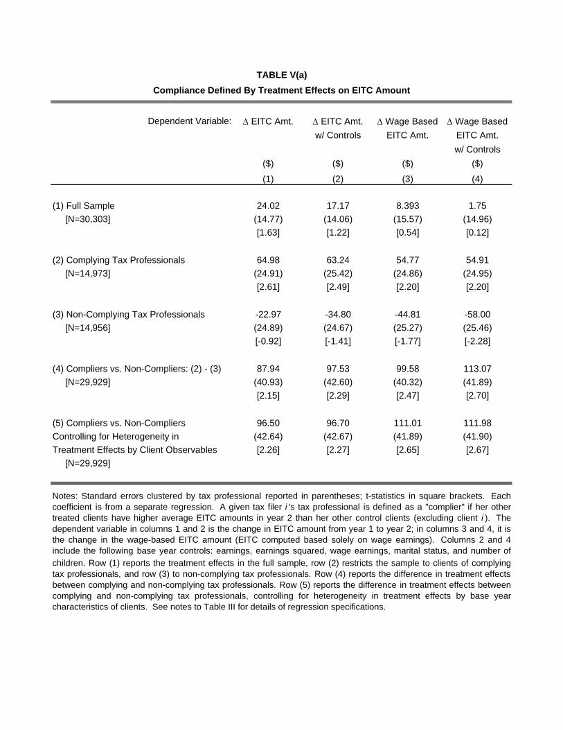
Dependent Variable: EITC Amt. EITC Amt. Wage Based Wage Basedw/ Controls EITC Amt. EITC Amt.

w/ Controls($) ($) ($) ($)

(1) (2) (3) (4)

(1) Full Sample 24.02 17.17 8.393 1.75 [N=30,303] (14.77) (14.06) (15.57) (14.96)

[1.63] [1.22] [0.54] [0.12]

(2) Complying Tax Professionals 64.98 63.24 54.77 54.91 [N=14,973] (24.91) (25.42) (24.86) (24.95)

[2.61] [2.49] [2.20] [2.20]

(3) Non-Complying Tax Professionals -22.97 -34.80 -44.81 -58.00 [N=14,956] (24.89) (24.67) (25.27) (25.46)

[-0.92] [-1.41] [-1.77] [-2.28]

(4) Compliers vs. Non-Compliers: (2) - (3) 87.94 97.53 99.58 113.07 [N=29,929] (40.93) (42.60) (40.32) (41.89)

[2.15] [2.29] [2.47] [2.70]

(5) Compliers vs. Non-Compliers 96.50 96.70 111.01 111.98Controlling for Heterogeneity in (42.64) (42.67) (41.89) (41.90)Treatment Effects by Client Observables [2.26] [2.27] [2.65] [2.67] [N=29,929]

TABLE V(a)

Notes: Standard errors clustered by tax professional reported in parentheses; t-statistics in square brackets. Eachcoefficient is from a separate regression. A given tax filer i 's tax professional is defined as a "complier" if her othertreated clients have higher average EITC amounts in year 2 than her other control clients (excluding client i ). Thedependent variable in columns 1 and 2 is the change in EITC amount from year 1 to year 2; in columns 3 and 4, it isthe change in the wage-based EITC amount (EITC computed based solely on wage earnings). Columns 2 and 4include the following base year controls: earnings, earnings squared, wage earnings, marital status, and number ofchildren. Row (1) reports the treatment effects in the full sample, row (2) restricts the sample to clients of complyingtax professionals, and row (3) to non-complying tax professionals. Row (4) reports the difference in treatment effectsbetween complying and non-complying tax professionals. Row (5) reports the difference in treatment effects betweencomplying and non-complying tax professionals, controlling for heterogeneity in treatment effects by base yearcharacteristics of clients. See notes to Table III for details of regression specifications.

Compliance Defined By Treatment Effects on EITC Amount

Year 2 variable for compliance def. Middle Income EITC Amount Middle Income EITC Amount

Base year controls in compliance def. No No Yes Yes

(1) (2) (3) (4)

(1) EITC Amt. ($) 173.92 0.044 127.94 0.101

(87.68) (0.029) (92.61) (0.038)[1.98] [1.52] [1.38] [2.64]

[N=29,351] [N=29,362] [N=29,346] [N=29,353]

(2) Wage-Based EITC Amt ($) 227.58 0.050 182.88 0.091(88.04) (0.029) (91.47) (0.038)[2.58] [1.72] [2.00] [2.42]

[N=29,351] [N=29,362] [N=29,346] [N= 29,353]

TABLE V(b)

Notes: Standard errors clustered by tax professional reported in parentheses; t-statistics in square brackets. Thistable uses continuous measures of compliance instead of binary definitions. Each coefficient listed is from a separateregression of the form shown in equation (3) in the text, which includes the treatment indicator, a continuous measureof tax professional compliance, and the interaction of these two variables. Each column of the table reports thecoefficient on the interaction between different tax professional compliance variables and the treatment indicator. Thedependent variable is the change in EITC amount from year 1 to year 2 in row (1), and the change in the wage-basedEITC amount in row (2). In all columns, the complying tax professional variable is defined for each client by excludingthat client himself. In column 1, the complying tax professional variable is defined as a continuous variable equal tothe fraction of other clients treated in year 1 who have middle income in year 2 (between $7,000 and $15,400) minusthe fraction of other control clients in year 1 who have middle income in year 2. In column 2, the complying taxprofessional variable is defined as a continuous variable equal to the average EITC amount in year 2 of other clientstreated in year 1 minus the average EITC amount in year 2 of other clients in the control group in year 1. Columns 3and 4 replicate the definitions in 1 and 2, but define the continuous measure of treatment effects on other clients usinga regression that controls for the following base year observables: earnings, earnings squared, wage earnings, maritalstatus, and number of children. We also control for the same base year variables and their interaction with thecompliance variable when estimating the regressions in columns 3 and 4.

Continuous Measures of Compliance

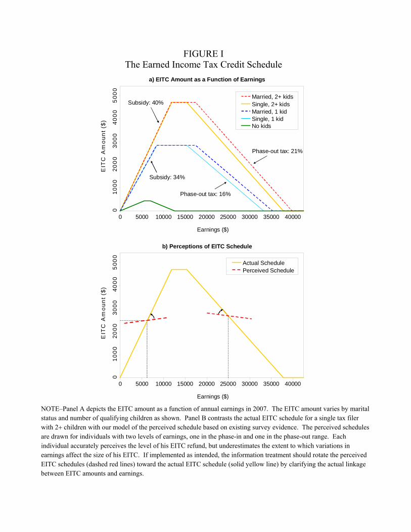
FIGURE IThe Earned Income Tax Credit Schedule

a) EITC Amount as a Function of Earnings

Earnings ($)

0 5000 10000 15000 20000 25000 30000 35000 40000

Subsidy: 34%

Subsidy: 40%

Phase-out tax: 16%

Phase-out tax: 21%

Single, 2+ kidsMarried, 2+ kids

Single, 1 kidMarried, 1 kid

No kids

EIT

C A

mou

nt

($)

010

0020

00

300

040

005

000

b) Perceptions of EITC Schedule

Earnings ($)

0 5000 10000 15000 20000 25000 30000 35000 40000

EIT

C A

mou

nt

($)

010

0020

00

300

040

005

000

Perceived ScheduleActual Schedule

NOTE–Panel A depicts the EITC amount as a function of annual earnings in 2007. The EITC amount varies by maritalstatus and number of qualifying children as shown. Panel B contrasts the actual EITC schedule for a single tax filerwith 2 children with our model of the perceived schedule based on existing survey evidence. The perceived schedulesare drawn for individuals with two levels of earnings, one in the phase-in and one in the phase-out range. Eachindividual accurately perceives the level of his EITC refund, but underestimates the extent to which variations inearnings affect the size of his EITC. If implemented as intended, the information treatment should rotate the perceivedEITC schedules (dashed red lines) toward the actual EITC schedule (solid yellow line) by clarifying the actual linkagebetween EITC amounts and earnings.

FIGURE IITime Spent Explaining the EITC to Clients Eligible for Treatment

Den

sity

Seconds

0.0

02.0

04.0

06

.00

8.0

1

0 100 200 300

NOTE–This figure is a histogram of the time spent (in seconds) by tax professionals on explaining the EITC to clientseligible for the information treatment. Time spent was recorded by the tax preparation software. The vertical line at 120seconds depicts the threshold above which tax professionals received $5 of compensation (per client) for explaining theEITC. The histogram is based on 20,809 observations. Each bin represents an interval of 3 seconds.

FIGURE IIIReturn Rates by Base-Year Income

Ye

ar

2 R

etu

rn R

ate

Year 1 Income ($1000)

Control Treatment

0.1

.2.3

.4.5

.6.7

.8.9

1

0 5 10 15 20 25 30 35

NOTE–This figure plots the fraction of base year clients who returned to H&R Block to file their taxes in year 2. Eachpoint represents the average return rate in a $1000 bin. The return rates are plotted separately for the treatment (solidred line) and control groups (dashed blue line).

FIGURE IVYear 2 Earnings Distributions: Complying Tax Professionals

a) 1 Dependent

020

0040

00

600

0

0 5000 10000 15000 20000 25000 30000 35000 40000

Ear

nin

gs D

en

sity

EIT

C A

mo

un

t ($)

Post-Treatment (Year 2) Earnings ($)

020

0040

00

600

0

0 5000 10000 15000 20000 25000 30000 35000 40000

Ear

nin

gs

Den

sity

EIT

C A

mo

unt

($)

Post-Treatment (Year 2) Earnings ($)

Control Treatment EITC Amount

Post-Treatment (Year 2) Earnings ($)

Control Treatment EITC Amount

b) 2+ Dependents

NOTE–These figures plot kernel densities of year 2 (post-treatment) income (sum of wage earnings andself-employment income) for the sample of individuals filing with a “complying” tax professional. A given tax filer i’stax professional is defined as a “complier” if she has a higher fraction of other clients (excluding client i) with middleincome (between $7,000 and $15,400) in the treatment group than the control group. The solid red curve shows theincome distribution for the treatment group; the dashed blue curve shows the income distribution for the control group.Panel A is for tax filers with 1 qualifying dependent for EITC purposes in the base year, while panel B is for tax filerswith 2 or more qualifying dependents. Each panel also shows the relevant EITC schedule (on the left y-axis). Thevertical lines mark the boundaries between the phase-in, peak, and phase-out ranges of the EITC.

FIGURE VYear 2 Earnings Distributions: Complying vs. Non-Complying Tax Professionals

00

.01

0.0

20

.03

0.0

4

02

000

400

06

000

0 5000 10000 15000 20000 25000 30000 35000 40000

Ear

nin

gs

De

nsi

ty (

x10

00)

EIT

C A

mo

unt

($)

a) 1 Dependent, Treatment Group

Post-Treatment (Year 2) Earnings ($)

02

000

40

0060

00

0 5000 10000 15000 20000 25000 30000 35000 40000

00

.01

0.02

0.0

30

.04

Ear

nin

gs

De

nsi

ty (

x100

0)

EIT

C A

mo

unt

($

)

Post-Treatment (Year 2) Earnings ($)

Non-Complying Tax Pros Complying Tax Pros EITC Amount

Post-Treatment (Year 2) Earnings ($)

Non-Complying Tax Pros Complying Tax Pros EITC Amount

b) 1 Dependent, Control Group

NOTE–These figures plot kernel densities of year 2 (post-treatment) income (sum of wage earnings andself-employment income) for tax filers with one dependent. The solid red curve shows the income distribution forindividuals filing with a “complying” tax professional; the dashed blue curve shows the income distribution forindividuals filing with a “non-complying” tax professional. See notes to Figure IV for the definition of “complying” taxprofessionals. Panel A is for the sample of individuals in the treatment group, while panel B is for the sample ofindividuals who were in the control group. Each panel also shows the relevant EITC schedule (on the left y-axis). Thevertical lines mark the boundaries between the phase-in, peak, and phase-out ranges of the EITC.

FIGURE VIYear 2 Earnings Distributions for Self-Employed Clients of Complying Tax

Professionalsa) 1 Dependent

Ear

nin

gs

Den

sity

0

0 5000 10000 15000 20000 25000 30000 35000 40000

EIT

C A

mo

unt

($)

200

040

00

600

0

Post-Treatment (Year 2) Earnings ($)

b) 2+ Dependents

Ear

nin

gs

Den

sity

020

00

400

06

000

0 5000 10000 15000 20000 25000 30000 35000 40000

EIT

C A

mou

nt (

$)

Post-Treatment (Year 2) Earnings ($)

Control Treatment EITC Amount

Post-Treatment (Year 2) Earnings ($)

Control Treatment EITC Amount

NOTE–These figures plot kernel densities of year 2 (post-treatment) income (sum of wage income andself-employment income) for tax filers who (a) had positive self-employment earnings in the base year and (b) filedwith a complying tax professional. See notes to Figure IV for the definition of “complying” tax professionals. Thesolid red curve shows the income distribution for the treatment group; the dashed blue curve shows the incomedistribution for the control group. Panel A is for the sample of individuals with one dependent, while panel B is for thesample of individuals with two or more dependents. Each panel also shows the relevant EITC schedule (on the lefty-axis). The vertical lines mark the boundaries between the phase-in, peak, and phase-out ranges of the EITC.

FIGURE VIIYear 2 Wage Earnings Distributions: Complying Tax Professionals

a) 1 Dependent

0

200

04

000

600

0

0 5000 10000 15000 20000 25000 30000 35000 40000

Ear

nin

gs

Den

sity

EIT

C A

mou

nt (

$)

Post-Treatment (Year 2) Wage Earnings ($)

b) 2+ Dependents

02

000

400

060

00

0 5000 10000 15000 20000 25000 30000 35000 40000

Ear

nin

gs D

ensi

ty

EIT

C A

mou

nt (

$)

Control Treatment EITC Amount

Post-Treatment (Year 2) Wage Earnings ($)

NOTE–These figures plot kernel densities of year 2 wage earnings (excluding self-employment income) for the sampleof individuals filing with a “complying” tax professional. See notes to Figure IV for the definition of “complying” taxprofessionals. The solid red curve shows the wage earnings distribution for the treatment group; the dashed blue curveshows the wage earnings distribution for the control group. Panel A is for tax filers with one dependent, while panel Bis for tax filers with two or more dependents. Each panel also shows the relevant EITC schedule (on the left y-axis).The vertical lines mark the boundaries between the phase-in, peak, and phase-out ranges of the EITC.

FIGURE VIIIYear 2 Wage Earnings Distributions: Complying vs. Non-Complying Tax

Professionals

Ear

nin

gs

De

nsi

ty (

x100

0)

EIT

C A

mou

nt (

$)0

200

04

000

600

0

0 5000 10000 15000 20000 25000 30000 35000 40000

a) 1 Dependent, Treatment Group

00.

010

.02

0.03

0.0

4

Post-Treatment (Year 2) Wage Earnings ($)

02

00

04

000

600

0

0 5000 10000 15000 20000 25000 30000 35000 40000

Ear

nin

gs D

en

sity

(x1

000

)

EIT

C A

mou

nt (

$)

Post-Treatment (Year 2) Wage Earnings ($)

Non-Complying Tax Pros Complying Tax Pros EITC Amount

Post-Treatment (Year 2) Wage Earnings ($)

Non-Complying Tax Pros Complying Tax Pros EITC Amount

b) 1 Dependent, Control Group

00

.01

0.0

20

.03

0.0

4

NOTE–These figures plot kernel densities of year 2 wage earnings (excluding self-employment income) for tax filerswith one dependent. The solid red curve shows the wage earnings distribution for individuals filing with a “complying”tax professional; the dashed blue curve shows the wage earnings distribution for individuals filing with a“non-complying” tax professional. See notes to Figure IV for the definition of “complying” tax professionals. Panel Ais for the sample of individuals in the treatment group, while panel B is for the sample of individuals in the controlgroup. Each panel also shows the relevant EITC schedule (on the left y-axis). The vertical lines mark the boundariesbetween the phase-in, peak, and phase-out ranges of the EITC.

3.Take-homeMessage

1. Fill in earnings, EIC amount

10,000 4,000

increasing

2. Explain and dot graph

4. Table

EXHIBIT IEITC Handout: 4 Step Explanation

APPENDIX EXHIBIT I(a)Information Treatment Screen #1 in H&R Block Software

APPENDIX EXHIBIT I(b)Information Treatment Screen #2 in H&R Block Software

Dear

Your earnings this year (in 2007) determine the size of your EIC refund next year. The EIC has 3 ranges: 1)Increasing, 2) Peak, 3) Decreasing.

The EIC (Earned Income Credit) gives tax refunds to working families. We want to explain how the EICworks to help you decide how much to work and earn this year. In 2006, you made $you are getting an EIC of $ in your tax refund.

In 2007 if you earnbetween:

Your EIC refund in2008 will be: If you earn $10 more, the EIC:

$0-$11,790 $0 up to $4,716 Increases by $4$11,790-$17,390 $4,716 Stays the same$17,390-$39,780 $4,716 down to $0 Decreases by $2.10

EIC Range

Increasing

DecreasingStays the Same

Note: The EIC does not affect any other credits or refunds you can get. This table applies to married joint filers with two or more qualifying children. Ifyour family situation changes in 2007, your EIC may also change (see IRS Publication 596). Changes in earnings may also affect other credits you areentitled to or taxes you may owe. Though the printed earnings and EIC amounts are based directly on your current tax return, the indication of yourposition on the graph is for illustrative purposes only.

and

WARD CLEAVER,

10000

You are in the ** increasing ** range of the EIC. Think about it like this: Suppose you earn $10 an hour. Because of the EIC you are really making $14 an hour. It pays to work more!

1984

APPENDIX EXHIBIT IIPrintout Given to Tax Filer

[Date]

[1st Name] and [1st Name] [Last Name][Address Line 1][Address Line 2][City] [State] [Zip]

Dear [1st Name],

Thank you for preparing your taxes with H&R Block this year. Even though it’s early, we want to provide important information that you may want to consider as you plan financially for next year. The EIC (Earned Income Credit) gives tax credits to working families. This year, you qualified for the EIC. This letter is a follow up to the EIC information your H&R Block tax professional shared with you when you had your taxes prepared. We want to remind you how the EIC works as you consider how much to work and earn this year.

As pictured on the graph below, the EIC has 3 ranges: 1) Increasing, 2) Peak, 3) Decreasing.

��

��

����

��

����

��

����

��

����

���

����

���

����

���

����

���

����

���

����

���

����

���

����

���

����

���

����

���

����

���

����

���

����

������

������

������

������

������

������

������

������

������

���������������������

���

����

����

����

�

Last year, you were in the increasing range of the EIC. Look at the table below. Will you be in the increasing range again this year? If yes, think about it like this: Suppose you earn $10 an hour. Because of the EIC, for each $10 you earn you could be eligible to receive an additional $4 in EIC – so it’s like you’re making $14 an hour. It pays to work more!

This table applies to single filers with two or more qualifying children. If your family situation changes in 2007, your EIC may also change (see IRS Publication 596). Many things can affect EIC, including changes in your family situation, other financial changes, or changes in tax laws. These changes may also affect your eligibility for other credits or deductions or taxes you may owe.

We hope you find the EIC information helpful. We look forward to continuing to provide tax and financial planning assistance to you in the future.

Sincerely,

Bernard M. Wilson Vice President Outreach & Business Development

�������������������������������������

��������������������������������

�����������������������������������

���������� ������������ ��������������� �����������������

���� ����������������� ������ �������������

���������� ����������������� ����������������� �����������������

APPENDIX EXHIBIT IIIFollow Up Letter Mailed to Tax Filer

Tax Professional Survey about the EIC Outreach Initiative March 2007 Office

Dear Tax Professional, As you know and thanks to your help, H&R Block has implemented an EIC outreach effort in Chicago where you have explained the Earned Income Tax Credit to our clients. In order to evaluate this initiative, we would like to ask you a few short questions about your experience. Please circle your response to each question below. 1) What proportion of your clients was interested in the EIC information?

a. Few (less than 25% of your clients)

b. Many (25% to 75% of your clients)

c. Most (over 75% of your clients) 2) Do you think Block should provide this EIC information to clients again in the future?

a. Yes

b. No

3) Is there anything else you would want to tell us about this EIC outreach or about how to make it work better?

a. No

b. Yes: Please explain below and/or on the back of this survey. 4) Did the explanation of EIC help your understanding of how the credit worked?

a. Yes b. No

Please return this survey to your office leader who will forward it to Block headquarters in the envelope provided to each office. Thank you for your participation in the EIC Outreach and in this survey. If you have questions, please contact Eileen McCarthy, at 816.854.4866.

APPENDIX EXHIBIT IV