AC 2007-3055: TEACHING OF ESSENTIAL MATLAB COMMANDS IN APPLIEDMATHEMATICS COURSE FOR ENGINEERING TECHNOLOGY

Ganapathy Narayanan, University of Toledo

© American Society for Engineering Education, 2007

Page 12.1365.1

Teaching of Essential MATLAB Commands in Applied Mathematics

Course for Engineering Technology

Abstract

The teaching of applied mathematics for students in the Engineering Technology (ET)

curriculum is always a challenge in terms of imparting the essential mathematical knowledge for

use in changing technological environments. In this paper, essential MATLAB commands in

the applied mathematics course for ET students are emphasized. Of several useful commands

available in MATLAB, only a select few, important and essential, commands are introduced to

enhance the understanding of the applied mathematical subject. In addition, this introduction of

essential MATLAB commands provides useful knowledge for ET students of the current and the

future technological approach to solve similar applied mathematical problems. The MATLAB

commands that are taught in the applied mathematics course are identified in this paper. In

addition, this paper gives notes on the use of each of these MATLAB commands through several

mathematical examples. The effects on the student's understanding of and on the enthusiasm

developed with the subject by such a teaching of these essential MATLAB commands are also

discussed in this paper.

Introduction

In this paper, the subject of MATLAB commands pertaining to the Applied Mathematics course

is discussed. Several textbooks exist for teaching Applied Mathematics1 and the use of

MATLAB2-5

. The teaching of the use of a select few MATLAB commands in conjunction with

the subject matter of the Applied Mathematics is undertaken in the ‘Applied Engineering

Mathematics’ course offered to the Engineering Technology (ET) students at the University of

Toledo, Toledo, Ohio. The discussion is limited to a select few MATLAB commands as

applicable to this applied mathematics course, and as to how these commands help in imparting

the subject of applied mathematics for ET students.

Several difficulties exist, both for undergraduate ET students in terms of understanding the

applied mathematics subject, and for the instructor in imparting the applied mathematical

knowledge required, to make students understand mathematical concepts and applied differential

equations with its solutions, within the semester time-frame. The 30 class hours (one semester)

are not sufficient for the instructor to make ET students understand and digest the subject matter

in order to make them proficient in applied mathematical analysis. Such a difficulty due to time

shortage cannot be avoided even if the course teaching hours are extended. This course is both

symbolic-intensive and numerical-intensive in terms of the applied mathematical analysis. If

symbolic tools and other computational aids are not made available, all students get bogged

down usually with many intermediate steps while solving for even the simplest ordinary

differential equation, and/or while producing appropriate solution plots manually that are of

interest. The MATLAB software, with its applied mathematical commands in its tool-box,

rescues the instructor and students in this course with many advantages for both, especially for

the ET student. Of course, some special virtual laboratory time need to be spent by students to

get trained in the use of these select MATLAB applied mathematics commands.

1

Page 12.1365.2

Thus, the ET student is trained in solving any applied mathematical problem without getting

distracted by many intermediate symbolic steps and/or by numerical calculations, and

subsequently, the student’s comprehension of the subject material is much better. The student

can then concentrate efforts in the overall design/analysis of an applied problem/system, leaving

symbolic/computational crunching to the virtual computer program (MATLAB). This increases

the student’s confidence and understanding of the applied mathematical subject, as is pertinent in

engineering. In addition, the benefits to the ET student after graduation are quite a lot from this

course in the sense that the knowledge of the use of MATLAB (software) as an assistant will

help the ET student in applied analysis, design and other areas of study, without extra efforts or

training, and especially, in his professional career.

There have been many successful attempts in several universities to teach the mathematical

subject using the symbolic software such as Maple or Mathematica. Of course, several texts do

exist in applied engineering mathematics with a parallel work shown using Maple6. In this

paper, a comparison is not done of all other software commands associated with these MATLAB

commands.

Select MATLAB Commands

The select few MATLAB commands taught in this applied mathematics course are classified

below according to eight important subject areas, for convenience of teaching. The eight areas

are chosen specifically to increase the students’ ability to remember MATLAB commands, and

to minimize any teaching difficulties of the applied mathematics subject in certain areas.

The eight categories of select MATLAB commands are:

a) Function Commands;

b) Plot Commands;

c) Symbolic Differentiation Command;

d) Symbolic Integration Command and its applications;

e) Taylor Series Command;

f) Laplace Transform Commands.

g) Ordinary Differential Equation Solver Command;

h) Partial Differential Equation Solver Command.

In this paper, only a few MATLAB output figures are shown. Other similar output figures can

be obtained easily by the reader or by the student, by typing in the MATLAB commands and its

examples on a computer.

Function Commands

The following basic types of functions are suggested to be studied, in detail, using MATLAB in

this applied mathematics course:

1. Exponential Function, bx

ae

2. Logarithmic Function, , ln( )a bx 10log ( )a bx

3. Trigonometric functions, sin ( )na bx s- , cos ( )n

a bx s- and tan ( )na bx s-

2

Page 12.1365.3

4. Power Functions, n

ax

5. Polynomial Functions, n

n

n

A xÂ

First, it is suggested in the virtual lab to understand the five ‘simple’ functions obtained by

using ,1, 1a b? ? 0s ? , & 1 for all n. Then, the values of constants ‘a’ and ‘b’ are

changed in each of the five basic functions to see how the simple functions changes in shape. In

general, it is known that an engineering technology student will use these functions 80% of time

in his professional career. So, his understanding of these functions and its x-y plots will help

clarify his understanding of derivatives and integrals of these functions.

1n ?n

A ?

The input commands for computing the five basic functional values for given values of ‘a’ and

‘b’ at ‘x’ are seen in MATLAB Command Window, as shown in Figure 1. The MATLAB

functional (f1, f2, f31, f32, f33, f4, f5) values output are shown in Figure 2. One can change the

values of parameters 'a', 'b' and 'n' in these functions as well as for the variable 'x' value.

Figure 1: MATLAB input commands for computing Basic

Functional Values

Plot Commands

In this course, MATLAB 2D plot commands are emphasized. These plot commands are,

namely, ‘plot’, ‘semilogx’ and ‘semilogy’. The 'plot' command produces the graphic plot of

tabular vector-valued variables x and y, with x-values along the 'linear' x-axis and y-values along

the 'linear' y-axis. One can define these x-variable and y-variable vectors either directly from the

ordered-pair values (table) or from computed y-functional values for the corresponding x-values.

The use of ‘plot’ command will be illustrated in this paper. The 'semilogx' and 'semilogy'

commands usage is similar to the 'plot' command. The 'semilox' command produces a plot with

x-values along x-log axis. The 'semilogy' command creates a plot with y-values along the y-log

axis. Figures 3 & 4 give the 'plot' command usage to generate an x-y plot. The 'plot' command

needs a minimum of two input arguments, namely x- and y-variables with vector values in them.

Only one function plot is generated here for illustration. In the class, virtual lab exercises to plot

all the five basic functions for various values of ‘a’ and ‘b’ are given.

3

Page 12.1365.4

Figure 2: MATLAB Basic Functional Values Output

Figure 3-A: MATLAB Table Plot Example

4

Page 12.1365.5

Figure 3-B: MATLAB Plot with two discrete valued vectors

(Table Plot)

Figure 4-A: MATLAB Functional Plot Example

5

Page 12.1365.6

Figure 4-B: MATLAB Plot of a Function

Symbolic Differentiation command

The MATLAB command for the symbolic differentiation is ‘diff’. This is a very powerful

command that is useful for taking derivatives of basic and composite functions of one or more

independent variables. The 'diff' command requires a minimum of two input arguments, namely,

the function to be differentiated as the first argument, and the variable in the function used for

differentiation. The MATLAB software does allow nesting of one 'diff' command inside of the

other 'diff' command. Mostly, in this applied course, only two independent variables are

considered. If double differentiation is needed of the same variable, then a third argument with a

value of '2' can be given. Figure 5 shows sample MATLAB example of taking symbolic

derivatives of functions of two variables. Of course, the derivatives of functions are also

functions of one or two variables, and they can be plotted, as explained above.

Symbolic Integration Command and its applications

The MATLAB command for the symbolic integration is ‘int’. This is also a very powerful

command that is useful in performing integration of basic and composite functions with respect

to one or two independent variables. The indefinite integral of 'int' command needs only two

input arguments, namely, the function to be integrated as the first argument, and the variable in

the function used for integration as the second. If the lower and upper limits of integration are

6

Page 12.1365.7

Figure 5-A: Use of MATLAB diff command

Figure 5-B: Use of MATLAB diff command

7

Page 12.1365.8

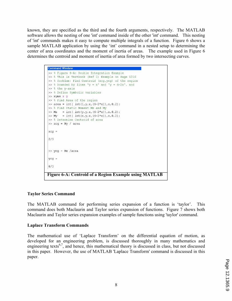
known, they are specified as the third and the fourth arguments, respectively. The MATLAB

software allows the nesting of one 'int' command inside of the other 'int' command. This nesting

of 'int' commands makes it easy to compute multiple integrals of a function. Figure 6 shows a

sample MATLAB application by using the ‘int’ command in a nested setup to determining the

center of area coordinates and the moment of inertia of areas. The example used in Figure 6

determines the centroid and moment of inertia of area formed by two intersecting curves.

Taylor Series Command

The MATLAB command for performing series expansion of a function is ‘taylor’. This

command does both Maclaurin and Taylor series expansion of functions. Figure 7 shows both

Maclaurin and Taylor series expansion examples of sample functions using 'taylor' command.

Laplace Transform Commands

The mathematical use of ‘Laplace Transform’ on the differential equation of motion, as

developed for an engineering problem, is discussed thoroughly in many mathematics and

engineering texts6,7

, and hence, this mathematical theory is discussed in class, but not discussed

in this paper. However, the use of MATLAB 'Laplace Transform' command is discussed in this

paper.

Figure 6-A: Centroid of a Region Example using MATLAB

8

Page 12.1365.9

The MATLAB ‘laplace’ command can transform a given time function into its corresponding

Laplace transform function. Similarly, the ‘ilaplace’ command can determine the inverse

Laplace transform of many useful functions defined in the Laplace domain. The use of ‘laplace’

and ‘ilaplace’ commands is shown in Figure 8. Both these commands require three input

arguments. The 'laplace' command requires the function as the first argument with 't' and 's' as

the second and third arguments. The 'ilaplace' command requires the transformed function as the

first argument with 's' and 't' as the second and third arguments.

Figure 6-B: Moment of Inertia Example using MATLAB

Ordinary Differential Equation Solver Command;

In MATLAB, it is possible to solve the ordinary differential equation (ODE) of any system

numerically for the system variable(s) in the time or the space domain. However, the solver

command 'dsolve' can be used to obtain 'symbolic' solutions of many ODE systems. Both 'direct'

and 'indirect' solutions of 'time' approaches of solving ODE are discussed in class. Of course,

deriving the 'direct' symbolic 'time' or 'space' solution of first and second order ODE is discussed

in detail, as mandated by the syllabus. Such mathematical details of solution are in texts1,6,7

.

MATLAB has several 'direct' ODE commands8 to solve for the system variable time or space

function, in a numerical form, with an associated numerical solution plot. Though these

commands are very useful for solving ODE numerically, such commands are not discussed in

9

Page 12.1365.10

this class. The numerical solutions of ODE are not part of the syllabus for this applied math

course, and hence, the numerical solution commands of ODE are not discussed in this paper.

Figure 7-A: Use of MATLAB taylor command

Figure 7-B: Use of MATLAB taylor command

10

Page 12.1365.11

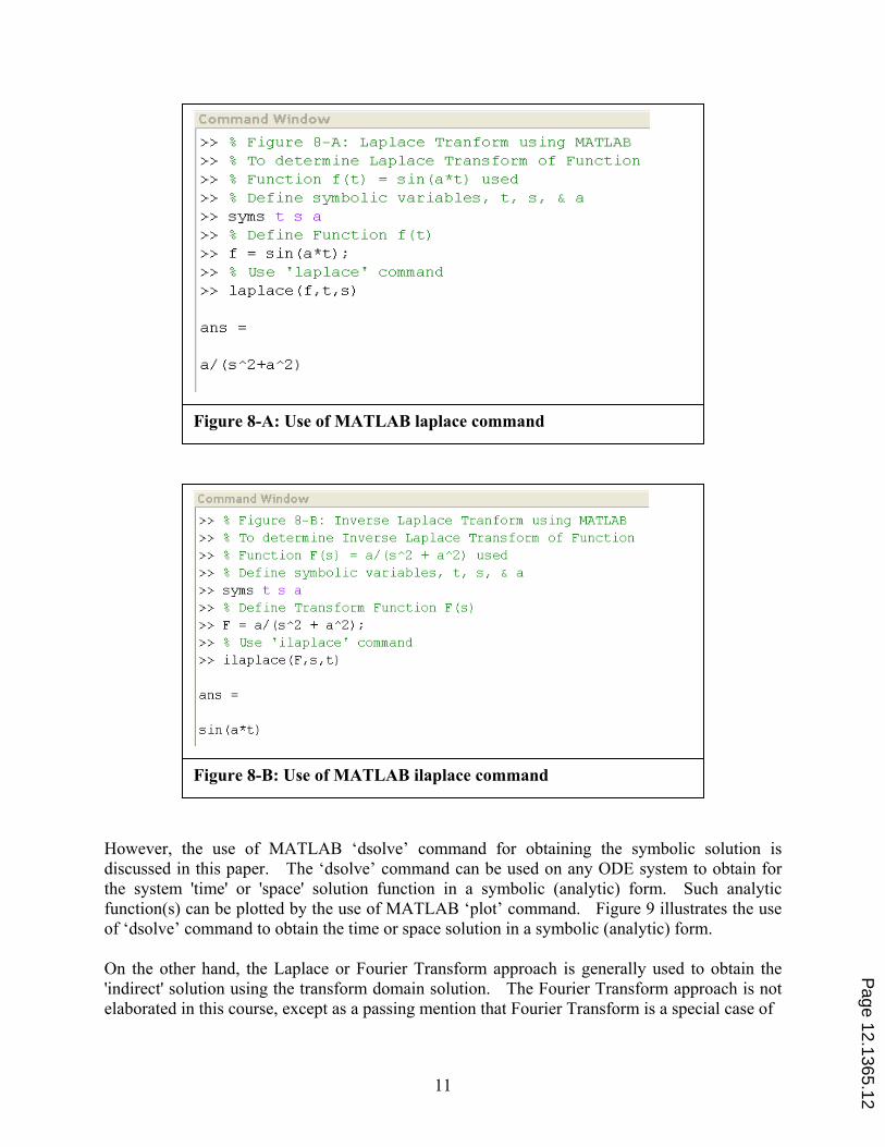
Figure 8-A: Use of MATLAB laplace command

Figure 8-B: Use of MATLAB ilaplace command

However, the use of MATLAB ‘dsolve’ command for obtaining the symbolic solution is

discussed in this paper. The ‘dsolve’ command can be used on any ODE system to obtain for

the system 'time' or 'space' solution function in a symbolic (analytic) form. Such analytic

function(s) can be plotted by the use of MATLAB ‘plot’ command. Figure 9 illustrates the use

of ‘dsolve’ command to obtain the time or space solution in a symbolic (analytic) form.

On the other hand, the Laplace or Fourier Transform approach is generally used to obtain the

'indirect' solution using the transform domain solution. The Fourier Transform approach is not

elaborated in this course, except as a passing mention that Fourier Transform is a special case of

11

Page 12.1365.12

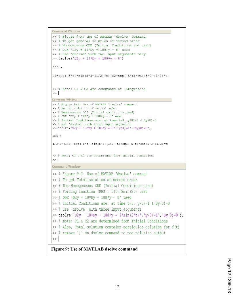
Figure 9: Use of MATLAB dsolve command

12

Page 12.1365.13

the Laplace Transform. The Laplace Transform approach of obtaining the solution for the first

and second order ODE is discussed in detail in the class.

Partial Differential Equation (PDE) Solver Command

This is a more advanced topic for the undergraduate engineering technology student, and hence,

it is not discussed in the course. However, this topic is left as an open topic for an advanced or

graduate student who can pursue this PDE subject when he needs it, either as an independent

study or take another course on PDE, with an associate training in the use MATLAB for solving

PDEs. There are many senior undergraduate and graduate courses offered at UT for the student

to advance his training in this direction. In any case, the commands that he learned in this

applied mathematics course will help him with his advanced training for solving partial

differential equation using the ‘dsolve’ or ‘pde’ commands, with ease.

MATLAB Resources: Additional MATLAB User Application resources are available at

www.mathworks.com/matlabcentral .

Classroom Use of select MATLAB commands

The above select MATLAB commands have been offered in the MET Applied Mathematics

course as a set of virtual laboratory exercises. There are about three computer laboratory

sessions used to present these select MATLAB commands, and the class room materials are

presented according to schedule such that the virtual laboratory work is integrated for student

experience of these subject materials.

The testing of understanding of the applied mathematics materials with the introduction of the

MATLAB laboratory exercises showed an increased interest and improvement among students’

understanding of the subject materials. There is definitely a success in the use of above

materials in the applied mathematics course. But a rigorous research was not done to assess the

percent of success in the applied mathematics course, with the introduction of above select

MATLAB commands virtual laboratory exercises. A comparative analysis of grades before and

after using this approach would give some perspective of the "goodness" of the technique, in

quantitative terms. Also, the impact of this approach of using select MATLAB commands on

the "deep" learning of ET students has not been studied.

Conclusions

The paper has been confined to the use of select MATLAB commands in the applied

mathematics course useful for the ET student. The MATLAB help facility can provide

additional information on the use of these individual commands. The paper has concentrated on

the application of these select commands as is taught in the applied mathematics course for ET

student. The elimination of the distraction of intermediate symbolic steps in the subject helps all

ET students concentrate and understand the important mathematical concepts taught in the

course. An additional advantage of learning the MATLAB control commands is with regard to

his increased ability to analyze/design any engineering system in his professional career, without

getting bogged down with many symbolic or numerical calculations. Of course, the use of

13

Page 12.1365.14

MATLAB commands did boost his ability to perform in obtaining symbolic solutions and/or

other calculations needed in other areas of his engineering study.

References

1) Peterson, J.C., “Technical Mathematics with Calculus, 3rd Edition”, Thomson Delmar Learning, 2004

2) Gilat, Amos, “MATLAB – An Introduction with Applications”, Second Edition, John Wiley, 2005.

3) Chapman, S. J., “MATLAB Programming for Engineers”, Second Edition, Brooks/Cole, 2002

4) Etter, D. M., Kuncicky, D. C., and Hull, D., “Introduction to Matlab 6”, Prentice Hall Engineering Source,

2002

5) Kuncicky, D. C., “MATLAB Programming”, Prentice Hall Engineering Source, 2004

6) Lopez, R.J., “Advanced Engineering Mathematics”, Addison-Wesley, 2001.

7) Kreyszig, E.,"Advanced Engineering Mathematics- 9th Edition", John Wiley, 2006

8) Polking, J.C., Arnold, D.,"Ordinary Differential Equations Using MATLAB", Prentice Hall, 2004

9) Farlow, S.J.,"Partial Differential Equations for Scientists and Engineers", Dover, 1993

Dr. G.V. Narayanan teaches at the University of Toledo, Toledo, Ohio. He can be contacted by email at

‘nara@utoledo.edu’.

14

Page 12.1365.15